Download for Brain Maps: Structure of the Rat Brain, 2nd

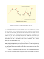
for Brain Maps: Structure of the Rat Brain, 2nd edition
Labeling Toolkit & Graphics Files (1998/1999)
CD-ROM User’s Manual
Contents
I. System requirements
II. Overview
III. Using Adobe Illustrator® files (Disk 1)
A. Downloading the files to your hard drive
B. Tips on making and printing illustrations
IV. List of downloadable files (Disk 1)
A. Interactive Brain Maps (Adobe Illustrator® 7 files)
1. Atlas of the adult rat brain
2. Flatmaps
3. Determining section angles
4. Database prototype
C. Other downloadable files
V. Labeling toolkit (Disk 2)
A. Installation
B. Introduction
C. Labeling toolkit manual
D. Graphics
E. Labels
VI. Purchaser’s agreement
CD-ROM User’s Manual
I. System requirements
PC
•
Hardware: 486 and higher, double-speed CD-ROM drive
•
Software: Windows 95, Windows 98 or Windows NT with a web browser such as
Netscape or MS Explorer installed. For Adobe Illustrator 7 on the PC, a Pentium
processor, 64 MB of RAM and a 19” color monitor are recommended.
Macintosh
•
Hardware: any Macintosh with a double-speed CD-ROM drive
•
Software: System 7 or higher, with a web browser such as Netscape or MS
Explorer installed. For Adobe Illustrator 7 on the Mac, a PowerPC is required, and at
least 48 MB RAM and a 19” color monitor are recommended.
Note: there is no Macintosh version of the Labeling Toolkit (on Disc 2).
2
II. Overview
This CD-ROM has two different parts. The first is a Label Toolkit for adding relatively
simple graphical information to the rat brain atlas maps and photomicrographs of the histological
sections from which they were traced. The Label Toolkit allows one to draw and to place text
over rasterized (bitmapped) maps and photos, and then to crop and size the figures for
publication (many journals can use the files directly for publication). In addition, the Label
Toolkit allows one to browse up and down through the stack of maps and photos to appreciate
how structures change progressively along the rostrocaudal or z-axis of the brain. The second
part of the CD-ROM contains vector graphics files of the Atlas that can be downloaded and used
in Adobe Illustrator® 7 (or other similar computer graphics applications), as well as high
resolution scans of the photomicrographs, and other useful files.
There are two versions of the vector-based Interactive Brain Maps atlas. One version is
complete, and features bilateral maps, a Nissl-stained section on one side, a list of abbreviations,
and two sets of coordinates—stereotaxic and physical. The other, simplified, version is designed
for mapping experimental results, and only contains the bilateral drawings of the brain. Because
these drawings are not rasterized, they can be modified in any way desired, and can be magnified
or reduced over a wide range without loss of resolution.
An extremely important feature of the Interactive Brain Maps is that they feature the use
of layers (when used in a graphics application such as Adobe Illustrator® 7). Layers are
analogous to perfectly aligned transparent overlays, and they can be viewed in any combination
and can be rearranged in any order. This powerful feature allows one to separate information (the
results of different experiments, or different features of the atlas such as abbreviations, cell
groups, and fiber tracts) in useful, creative ways, and then view or hide, lock or unlock, and
delete or add individual layers. As one works with these complex drawings, the value of layers
becomes increasingly obvious, especially when taking advantage of the ability to move graphical
elements between layers, and to duplicate information in more than one layer.
Another important feature of vector graphics is that they can be printed at very high
resolution (for example, commercial Imagesetters can typically print at 2400 to 3600 dpi
resolution). And this is true even if one crops out a small part of a drawing and magnifies it
considerably and/or makes a very large print.
3
III. Using Adobe Illustrator® files (Disk 1)
In this day and age, knowledge of how to use one of the major computer graphics
applications is basically essential for anyone publishing neuroanatomical illustrations. The
downloadable files provided here were created with Adobe Illustrator® 7 and Adobe
Photoshop® 4. Similar versions of these applications are available for the PC and Mac, and the
user interfaces for both of them share many features in common. Adobe Photoshop® is designed
primarily to work with bitmapped images (such as videophotos or scanned images and films),
whereas Adobe Illustrator® is designed to create vector-based drawings, which may be
combined with placed bitmapped art (e.g., from Photoshop) for the construction of illustrations
for printing, making 35 mm. slides, and publication. There are several other popular computer
graphics applications, including Macromedia FreeHand® 8, Deneba Canvas® 5, and
CorelDRAW® 8, and Adobe Illustrator® files usually can be opened and worked on in them
(contact manufacturer if procedure is not obvious).
The Adobe Illustrator® tutorial is an essential and enjoyable prerequisite for those not
comfortable with the program.
A. Downloading the files to your hard drive
Open the “start.htm: file on Disc 1 in your web browser. The web based interface will
bring you to listings of the files that are discussed in the following pages of this booklet. The
downloadable files in Adobe Illustrator format (*.ai and *.esp) can be downloaded directly to
your hard disc by clicking your right mouse button (Windows) or holding the mouse button
(Macintosh users), and chosing the “save this link” option. It is also possible to change the
“preferences” settings of your browser, under “applications”, and to chose the option “save to
disc” or “start application”. Some browsers may have a QuickTime plug-in installed that opens
TIFF images on screen. When this happens, the “save as” option in the “File” menu can be used
to save the TIFFS to hard disc.
While these files have broad applications, their use in published figures should
acknowledge that they are based on Brain Maps: Structure of the Rat Brain, second revised
edition (Swanson, 1998).
4
B. Tips on making and printing illustrations
The general philosophy of using computer graphics applications for producing
neuroanatomical illustrations is outlined in section IVB3 of the book. The following discussion is
based on using Adobe Illustrator® 7, although the general principles apply to other popular
applications.
It is necessary at the outset to learn how to use the layers manager or palette. Layers are
like a perfectly aligned stack of transparent overlays. Their stacking order can be changed at any
time, they can be viewed in any combination by hiding individual layers, and any combination of
layers can be chosen to print. One obvious use would be to place the results of a tracing
experiment in a layer over an atlas template, or the results of two tracing experiments in two
layers over an atlas template (with the results of each experiment in a different color). It is
important to remember that objects in a layer “block out” or obscure all objects in layers below it
in the stacking order, just as in a stack of transparent overlays. This must be considered when
changing the stacking order of layers. It is also useful to know that objects can be moved from
one layer to another simply by selecting the object (or objects) and moving the resulting dot in
the layers palette to the desired layer. Similarly, an object(s) in one layer can be duplicated
(select, copy, paste in front) and then moved to any desired layer, so the same object appears in
two layers.
Drawing in a layer is, of course, a basic operation or skill that is usually the most
frustrating part of learning a computer graphics application. Like pen and ink drawing, it requires
practice, and can always be improved. Curved lines in Illustrator are based on creating Bezier
curves, which are smooth and mathematically defined (explaining why they are essentially
infinitely scalable without loss of resolution).
To learn how to use the pen tool for drawing, first read the Illustrator User’s Guide.
Basically, curved lines (paths) are drawn by creating a series of smooth anchor points, each with
a direction line on either side, and a direction point on the end of each direction line (Figure 1).
These points and lines are used to edit in a very precise way paths that have already been drawn.
Several rules help produce the most esthetically pleasing drawings. (1) Use the minimum number
of anchor points consistent with the desired line. This requires practice, and planning ahead
while drawing. It is essential that one does not try to draw too fast; think deliberately about what
5
you are drawing. It is instructive to see how Illustrator draws a circle. To do this, use the circle
tool, and then select it to see the anchor points, direction lines, and direction points. Note only
four anchor points, and equally spaced direction points. In general, use fewer anchor points on
less curved regions of a path. (2) Keep facing direction points for adjacent anchor points on the
same side of a path. And (3), try to follow the “thirds rule:” In the space between two anchor
points, each direction line, and the distance between the two direction points, should be
approximately equal (that is, each should be about a third of the distance). This is perfectly
shown in the way Illustrator draws a circle.
Paths can also contain corner anchor points. The path in Figure 1 was drawn with six
anchor points, four of them smooth (a-d) and two of them corner (e, f). Corner anchor points are
created by clicking (rather than clicking and dragging) and are used to create angles in a path
(use the rectangle tool to create a rectangle or square and note that it consists of only four corner
anchor points).
Learn how to use all of the tools in the toolbox palette. They are used for editing paths, as
well as for scaling, magnifying, rotating, reflecting, and skewing, for placing and modifying text,
6
and so on. Also learn how to change line thickness and color, and how to create dashed lines.
The pencil tool is useful for drawing irregular lines (such as PHAL-labeled axons),
although you will note that even these paths are actually Bezier curves that Illustrator creates for
you, and may thus be edited like paths drawn with the pen tool. Although it takes essentially no
practice to use the pen tool, it is also not appropriate to use when drawing smooth paths.
Symbols (circles, squares, and so on) from the Symbol font are usually best to use for
items showing the location of labeled neurons and so on. Although they require more memory
than symbols created with Illustrator paths, they maintain their relative positions when maps are
rescaled.
For most routine drawing, it is helpful to show three Adobe Illustrator® 7 palettes along
the top of the Window: one with the Layers subpalette, one with the Stroke, Color, and Swatches
subpalettes, and one with the Character and Paragraph subpalettes.
There is a simple rule to follow when printing vector graphics: The more resolution the
better. Publication quality prints typically require 800-1200 dots per inch (dpi) resolution when
shading and thin lines are involved, and the best prints are made with a 2400 dpi Imagesetter
(obtained from a commercial service provider). At this time, high resolution Imagesetters do not
produce multiple color prints; on the other hand, high resolution laser printers (600, or better yet
1200 dpi) produce adequate proofs of color drawings at rather high speed (but not photoquality
bitmapped images). Recall that there are 72 points (a measure of line thickness and font size) to
an inch when designing artwork.
7
IV. List of Downloadable Files (Disk 1)
A. Interactive Brain Maps (Adobe Illustrator® 7 files)
1. Atlas of the adult rat brain
a. Atlas levels (sagittal)
b. Brain Maps, Computer Graphics Files 2.0 /COMPLETE
c. Brain Maps, Computer Graphics Files 2.0 /Map only
2. Flatmaps
a. Rat CNS flatmap 2.0
b. Cortex sections on flatmap (rat)
c. Unfolded hippocampal formation (rat)
d. Human CNS flatmap 1.0
3. Determining section angles
a. Sagittal and dorsal brain views
b. Interbrain section plane (practical example)
4. Database prototype
a. Sample database (Level 19)
b. Sample data layer (Level 19)
B. Other downloadable files
1. Scanned atlas plates—300 dpi (Adobe Photoshop® TIFF files)
2. Archival material (Adobe Illustrator® files)
a. Brain Maps, Computer Graphics Files 1.0 (1993)
b. Brain Maps (first edition), shaded drawings (1992 book)
8
A. Interactive Brain Maps (Adobe Illustrator® 7 files)
1. Atlas of the adult rat brain
There are three files or sets of files dealing with the Atlas. One file is called Atlas levels
(sagittal), and it is a midsagittal view of the rat brain showing the location of the 73 atlas levels
(Fig. 10 in the book). The two sets of files contain the individual atlas levels themselves. Brain
Maps, CGF 2.0/COMPLETE (Brain Maps, Computer Graphics Files 2.0/COMPLETE) is the
second edition of Brain Maps, Computer Graphics Files (Elsevier, Amsterdam, 1993; included
in archival material, below) and is a truly interactive atlas, with bilateral maps, accompanying
photomicrographs of the Nissl-stained sections, a list of abbreviations, and two coordinate
systems; and Brain Maps, CGF 2.0/Map only, which contains only bilateral atlas maps for
creating neuroanatomical data overlays. The drawings are all at the same scale, are in register,
and are designed to fit on a piece of US letter size (8.5 x 11 in.) paper when printed.
Individual atlas levels in Brain Maps, CGF 2.0/COMPLETE are easy to use when opened
in Adobe Illustrator® 7, with the Layers palette showing and extended to display all six layers
(after opening a file, select Fit in Window in the View menu). Simply hide and show different
combinations of layers. When printing, remember that you have the option to print or not to print
each layer. It is also simple to move different components of the atlas drawing into different
layers. This is easy because different components are grouped, and can be selected with the
selection tool (black arrow, upper left). Create a new layer and move the selection to it. The atlas
drawing layer has the following groups, which must be stacked in the following order of layers
(from bottom to top): (1) cell group outlines, (2) fiber tracts (shaded or filled), (3) fiber tract
subdivisions (lines or paths), and (4) brain outlines and ventricles. The yellow mask layer just
below the atlas layer is useful when one atlas level is placed partly over another in a composite
illustration because the mask blocks out the part of the bottom atlas level that lies directly
underneath the top atlas level (Figure 2). The mask is a compound path, so that the ventricles are
like holes in the tissue section that are not masked. Of course the fill color of the mask can be
changed to anything desired, including most often white for publication.
Individual atlas levels in Brain Maps, CGF 2.0/Map only are much simpler; they consist
9
only of the atlas layer of Brain Maps, CGF 2.0/COMPLETE (and thus have no mask). They are
very convenient for straightforward mapping of neuroanatomical data in a new overlying layer or
layers.
Cropping part of an atlas level in Brain Maps, CGF 2.0/Map only for a final illustration is
relatively straightforward. The easiest way to start involves creating a rectangle of the
appropriate size and location, locking it; and then using the scissors tool to cut lines in the atlas
drawing along the border of the rectangle. Then select lines and text outside the rectangle and
10
delete. The only problem arises when certain oddly-shaped filled objects (fiber tracts) are cut in
such a way that the fill pattern is disrupted. When this happens, some redrawing (usually forming
a closed path at the corner of the locked rectangle) is necessary (Figure 3); this is especially easy
if the fiber tracts are placed in a separate layer for editing, and then returned to the atlas layer
(between cell groups and fiber tract divisions groups; the stacking order of selected objects, such
as fiber tracts, can be altered from the Arrange submenu in the Object menu).
Note that all atlas levels in both Brain Maps, CGF 2.0/COMPLETE and Brain Maps,
CGF 2.0/Map only have a layer called physical coordinates/dbf. This layer contains a bounding
blue rectangle, which is a database fiducial (dbf). It has two purposes. First, it is perfectly in
register along the z-axis of the brain for all 73 atlas levels. Taken together, they can be thought of
in three dimensions as forming the sides of a box around the brain. And second, the blue
rectangle should be copied to data layers that are used in neuroanatomical graphical databases; it
assures perfect alignment of the data layers (in the absence of the atlas layer, for example)—
hence the name “database fiducial” (see section IVC in the book and section E4b below).
2. Flatmaps
The purpose of these design aids is to provide standardized templates for illustrating all
neural systems in a uniform way (see section V in the book, as well as the frontispiece, which
11
was created with the Rat CNS flatmap). Rat CNS flatmap 2.0 is an updated, computer graphics
version of Figure 7 in the first edition of Brain Maps: Structure of the Rat Brain (Elsevier,
Amsterdam, 1992), which did not contain pathways. Open this file in Adobe Illustrator® 7, show
the Layers palette and all of its contents, and then begin near the bottom of the Layers palette to
show and hide the various layers to see what they contain (general contents are indicated by the
name in the Layers palette).
The Rat CNS flatmap 2.0 file contains most of the major known pathways in the rat,
placed in a standardized position. This version of pathway placement over the flatmap should be
considered provisional—as a “work in progress” that will undoubtedly require considerable
refinement in the future.
To create a circuit diagram, view the SIMPLE OUTLINE (for pathways) layer, and hide
all the others. View a layer containing pathways of interest. Select, copy, and paste in front, then
move duplicated pathways to a NEW DRAWING layer. Fine tune the ends of pathways with the
pen tool, show cell groups of interest (e.g., by a circle created with the symbols font), arranging
the circuit in an aesthetic way (choose appropriate line thickness, color, and so on). Repeat this
process until you have all of the pathways necessary for the circuit diagram, and refine the
overall design. Labels are provided in the footprint abbreviations layer. Near the end, copy your
NEW DRAWING layer(s) and an appropriate outline layer to a new file (lock all other layers and
select all), where components may be placed in layers as desired, and the diagram can be printed
from a much smaller file.
The approximate location of atlas sections through the cerebral cortex are shown in
relation to the Rat CNS flatmap 2.0 in a file called Cortex sections on flatmap (this drawing is
250% larger than the flatmap itself). The idea here is to provide a qualitative way to map the
distribution of neuroanatomical data onto a flattened representation of the cerebral cortex.
Variations in the contour pattern are a reflection of curvature on the surface of the intact cerebral
cortex. Each line in the contour map is derived from the cortical surface of a particular atlas level
(as indicated).
A flatmap of the rat hippocampal formation (Unfolded hippocampal formation) is also
provided. Its shape is not derived from the Rat CNS flatmap 2.0, but rather from the surface of a
three-dimensional model of the hippocampal formation (Swanson, L.W., J.M. Wyss & W.M.
12
Cowan (1978) An autoradiographic study of the organization of intrahippocampal association
pathways in the rat. J. Comp. Neurol., 181:681-716). The original map has been modified in light
of more recent data (e.g., Risold, P.Y. & L.W. Swanson (1996) Structural evidence for functional
domains in the rat hippocampus, Science, 272:1484-1486) and understanding; a full description
is in preparation. As with the above files, different types of information are in different layers.
Finally, a simple Human CNS flatmap 1.0 file is provided for comparison with the rat.
This file was used to produce Figure 2, and the accompanying poster, in Swanson, L.W. (1995)
Mapping the human brain: Past, present, and future, TINS, 18:471-474. The major feature of
interest here is a flatmap of Brodmann’s areas in the cerebral cortex.
3. Determining section angles
It is very useful for mapping to have a good estimate of how the plane-of-section of an
experimental brain compares with that of the standard atlas plane-of-section (see Figure 7 in the
book). The solution presented here is graphical. Assuming that the midline of the experimental
sections is set to vertical, there are two degrees of freedom: A dorsoventral difference in planeof-section, and a mediolateral difference in plane-of-section. The former is seen as a difference
in the sagittal view, whereas the latter is seen in a dorsal (used here) or ventral view of the brain.
The basic principle is to determine how particular pairs of fiducial points differ between the atlas
and an experimental brain.
The two files presented here are designed to determine plane-of-section for structures
located in or near the interbrain. For other parts of the brain, the user should determine
appropriate fiducials (see pp. 27-30 in the book, and the file Sagittal & dorsal brain views).
Interbrain section plane (practical example). This file is a 150% enlargement of the
interbrain region from the file Sagittal & dorsal brain views (which displays the same fiducial
points). It contains sagittal and dorsal views of the interbrain region of the atlas brain (which was
embedded in celloidin, and thus shrank considerably; see section IIIA in the book) with the series
of atlas sections superimposed. It also contains sagittal and dorsal views of a brain prepared by
frozen sectioning (the atlas brain was scaled to approximate the coordinates in Paxinos and
Watson, 1986; see section IIIA in the book).
The basic principle is to align a regularly spaced Nissl-stained series of sections from the
13
experimental brain (frozen sections) on the frozen-sectioned brain outlines here, basing the
alignment on the position of fiducial points. A series of lines representing the experimental series
is constructed to scale (using the rulers), and then rotated relative to the standard series, based on
the position of the fiducials. This is a graphical solution that does not require mathematical
calculations, although the angles can of course be determined.
One practical strategy to determine the plane of the experimental brain is first to
determine how many sections from the experimental series fit between two widely-spaced
fiducials, such as the rostral tip of the suprachiasmatic nucleus (SCH) and the caudal end of the
mammillary recess (V3mr). This number of sections is fitted between the two fiducials (e.g., by
moving, rotating, and scaling the sample frozen section series provided in the Layers palette) in
the drawing of the MIDSAGITTAL VIEW. Second, to determine the “dorsoventral” error in
plane-of-section, observe which section in the experimental series passes through a dorsal
fiducial (e.g., the caudal anterior commissure, ac), and which section passes through a fiducial
more or less ventral to the first (e.g., the rostral SCH). Rotate the group of experimental sections
to reproduce these relationships. If necessary, rescale the set of experimental sections so that the
correct number of sections still stretches between the rostral and caudal fiducials determined in
the first step. One now sees how the experimental series is oriented relative to the atlas sections.
And third, to determine the “mediolateral” error in plane of section, repeat the above process
using the drawing of the DORSAL VIEW, with appropriate fiducials. Obviously, error will be
reduced by using fiducials that are as far apart as practical (see section IVB in the book).
4. Database prototype
A web-based browser for neuroanatomical data mapped onto Brain Maps, CGF 2.0 is
under development (see Dashti et al. (1997) NeuroImage, 5: 97-115). The two files in this folder
show how data layers from this database could be used in the layer manager of Adobe
Illustrator® 7. The basic idea is discussed in section IVC of the book. Note that file Sample data
layer (Level 19) contains only the data itself, and a blue bounding rectangle, the database fiducial
(dbf), which is found in every atlas level (in the layer called physical coordinates/dbf). It can be
copied, pasted in front, and moved to any other (data) layer.
14
C. Other downloadable files
Several other useful file sets are provided on the CD-ROM.
First, a set of atlas photomicrographs scanned at relatively high resolution (300 dpi) is
provided as Photoshop TIFF files; they should be viewed in Adobe® Photoshop. The atlas
photomicrographs provided with Brain Map, CGF 2.0 /COMPLETE were scanned at roughly
monitor resolution (72 dpi) for speed of manipulation.
And second, two folders are provided in the Archival material section. One folder
contains the files of Brain Maps, Computer Graphics Files 1.0 (Elsevier, Amsterdam, 1993), and
the other folder contains the original files used to print the shaded drawings in Brain Maps:
Structure of the Rat Brain (Elsevier, Amsterdam, 1992). These files must not be confused or
mixed with Brain Maps, Computer Graphics Files 2.0 supplied above. They are provided for
historical reasons, so that interested readers can compare changes in the atlas from the first to the
second edition (e.g., a considerable amount of data was published with the first edition as
templates).
V. Labeling toolkit (Disk 2)
A. Installation
The Labeling Toolkit runs under Windows 95, Windows 98, and Windows NT only.
To install the Labeling Toolkit, choose the “start” option in Windows, go to the “Install”
directory, select “setup.exe”, and follow the instructions on screen.
B. Introduction
The Labeling ToolkitTM is an image markup tool for:
•
Reading in sets of images
•
Adding shapes, lines, arrows, text, and pictures to highlight important information
•
Capturing screen images
•
Printing images
The interface of the Labeling Toolkit is very simple. Three buttons in the upper left
corner of the interface let you load and save files, capture screen images, print images, and open
and close two small windows. In the viewing area on the right, you can view and mark-up the
15
images. The Features list on the left displays a list of the mark-ups (features). Using the Features
list, you can create groups of features, toggle on and off the display of images and features, and
rename and delete features.
In addition to the main window, the interface has two small windows—the Navigation
window and the Palette.
The Navigation window lets you move through the image set one image at a time, or
“play” through the set in forward or reverse.
You can open and close the Navigation window by clicking the navigation button in the
upper left corner of the interface.
C. Labeling toolkit manual
In the “User Guide” directory on the CD-ROM you will find three versions of the
complete Toolkit user’s manual: two versions in HTML format (*.htm), one including screen
shots (UserGuide.htm), that can be viewed in any web browser; and a text version
(UserGuide.txt), without screen shots, that can be opened in any word processor.
D. Graphics
Atlas
The “Atlas” directory contains Nissl stain sections of all 73 rat brain levels in Adobe
Illustrator file format. These files cannot be loaded into the Labeling Toolkit. These are
archival/original versions of the bitmap versions in other directories.
BM-files
These are Adobe Illustrator files of all 73 Brain Maps drawings. These are
archival/original versions of the bitmap versions in other directories and cannot be loaded in the
Labeling Toolkit.
Toolkit Images
This directory contains bitmap versions of all Atlas and BM-files in two different
16
resolutions, 72 dpi and 300 dpi. These are the files that can be used in the Labeling Toolkit. The
300 dpi files are very large and slow to load and manipulate and need a large amount of RAM.
Image stack loading is not recommended. The application may crash if too many images are
loaded. The 72 dpi images are the best images for the Toolkit.
The 300 dpi images are zipped in png format, the 72 dpi images are TIFFs.
E. Labels
The Label.lbl file on the CD-ROM can be loaded when the text button on the toolbar is
selected. The label dialog box comes up. Here you can load the label file and select labels from
the list box.
VI. Purchaser’s agreement
This is an agreement between Elsevier Science B.V. and the purchaser of Brain Maps.
The purchaser recognizes Elsevier Science B.V. as the publisher and owner of the title of
and the copyright in and of all other rights in and to the print atlas Brain Maps; Structure of the
Rat Brain, 2nd Edition, and the accompanying two CD-ROM disks. Elsevier Science B.V.
herewith grants to the purchaser a limited nonexclusive license to use those two CD-ROM disks
(“BM CD-ROMs”), subject to the following terms and conditions.
The purchaser agrees to the following:
1. The purchaser shall not make any copy of the BM CD-ROMs, except for one (1) backup copy for security purposes only.
2. The purchaser shall not publish, republish, assign, sell, lend, or otherwise make the
BM CD-ROMs, or parts thereof, available to third parties.
3. The purchaser shall not use the BM CD-ROMs on more than one computer at the same
time. If BM CD-ROMs are to be used on a network electronic mail system, or file server,
permission is required from and additional fees are due to Elsevier Science B.V. A list of the
17
applicable user fees is available from Elsevier Science B.V.
4. While these files have broad applications, the purchaser should acknowledge that they
are based on Swanson, L.W. (1998/1999) Brain Maps: Structure of the Rat Brain, 2nd Edition,
Elsevier, Amsterdam.
If the purchaser performs any of the prohibited acts, the purchaser will infringe Elsevier
Science’s right and thereby cause damage to Elsevier Science’s interests. Elsevier Science B.V.
intends to enforce its rights to the fullest extent possible.
From the inside front cover of the booklet:
“Copyright © 1998/1999 Elsevier Science B.V., Amsterdam, The Netherlands. All rights
reserved. No part of this publication may be reproduced, stored in a retrieval system or
transmitted in any form by any means, electronic, mechanical, photocopying, recording or
otherwise, without the prior written permission of the publisher: Elsevier Science B.V., P.O. Box
521, 1000 AM Amsterdam, The Netherlands.
No responsibility is assumed by Elsevier Science B.V. for any injury and/or damage…
N.B. Please see ‘Purchaser’s Agreement’ on p. 23.”
18