Download GenAlEx 6.5 Guide (pdf 2.7 mb) - Australian National University

A Comprehensive
Guide to:
!"#
!"##$%&'%"#("
Written by Michaela D.J. Blyton
and Nicola S. Flanagan
http://biology.anu.edu.au/GenAlEx/
A Guide to GenAlEx 6.5
2 of 131
Table of contents
Table of contents ....................................................................................................................... 2!
Introduction............................................................................................................................... 5!
GenAlEx 6.5....................................................................................................................................... 5!
User registration and citation of GenAlEx 6.5 ............................................................................... 6!
GenAlEx 6.5 Installation .................................................................................................................. 6!
About this Manual ............................................................................................................................ 7!
Manual Style...................................................................................................................................... 7!
Disclaimer .......................................................................................................................................... 7!
The GenAlEx Environment ...................................................................................................... 8!
Overview ............................................................................................................................................ 8!
Data Limits ........................................................................................................................................ 8!
Input ................................................................................................................................................... 8!
Output ................................................................................................................................................ 9!
Standard Data Parameter Dialog Box ............................................................................................ 9!
Options ............................................................................................................................................. 11!
Data format for GenAlEx ....................................................................................................... 13!
Numerical Format .......................................................................................................................... 13!
Missing Data .................................................................................................................................... 13!
Sample Labels ................................................................................................................................. 13!
Data Structure ................................................................................................................................. 14!
Data Parameters and Labels.......................................................................................................... 14!
Data Formats ................................................................................................................................... 15!
Template .......................................................................................................................................... 22!
Create ............................................................................................................................................... 23!
Parameters....................................................................................................................................... 25!
Data .................................................................................................................................................. 27!
Frequency Based Statistical Procedures ................................................................................ 29!
Frequency ........................................................................................................................................ 29!
Disquil .............................................................................................................................................. 37!
HWE................................................................................................................................................. 37!
Paired Biallelic LD .......................................................................................................................... 38!
G-Statistics....................................................................................................................................... 40!
Shannon ........................................................................................................................................... 43!
Pairwise Pops .................................................................................................................................. 43!
Partition ........................................................................................................................................... 46!
A Guide to GenAlEx 6.5
3 of 131
Relatedness ...................................................................................................................................... 50!
Pairwise ............................................................................................................................................ 50!
Pops Mean ....................................................................................................................................... 52!
Multilocus ........................................................................................................................................ 54!
Assignment ...................................................................................................................................... 57!
Pop Assign ....................................................................................................................................... 57!
Sex Bias ............................................................................................................................................ 59!
Distance Based Statistical Procedures ................................................................................... 61!
Distance ............................................................................................................................................ 61!
Genetic Distance.............................................................................................................................. 61!
Geographic Distance ....................................................................................................................... 64!
Genetic by Pop ................................................................................................................................ 67!
Matrix Manipulation ...................................................................................................................... 67!
AMOVA ........................................................................................................................................... 69!
Mantel .............................................................................................................................................. 74!
Paired ............................................................................................................................................... 74!
Multi ................................................................................................................................................. 75!
Compare .......................................................................................................................................... 76!
PCoA ................................................................................................................................................ 77!
Spatial Autocorrelation .................................................................................................................. 79!
Single Pop… .................................................................................................................................... 79!
Multiple loci… ................................................................................................................................. 84!
Multiple Pops… .............................................................................................................................. 86!
Multiple Pop Subsets … ................................................................................................................. 88!
Multiple Dclass … ........................................................................................................................... 90!
Pops as Dclass … ............................................................................................................................. 92!
2D Local Spatial Analysis (2D LSA) ............................................................................................. 93!
Nearest Neighbor Distance (NN Dist) ........................................................................................... 96!
Clonal ............................................................................................................................................... 98!
TwoGener ...................................................................................................................................... 101!
Raw Data Editing .................................................................................................................. 102!
Import Data ................................................................................................................................... 102!
Genotypes ...................................................................................................................................... 102!
Sequences ....................................................................................................................................... 103!
GenePop file .................................................................................................................................. 106!
Tab Delimited ................................................................................................................................ 106!
Space Delimited ............................................................................................................................. 107!
A Guide to GenAlEx 6.5
4 of 131
Folder Nexus Alignments ............................................................................................................. 107!
Raw data ........................................................................................................................................ 108!
Combine Data................................................................................................................................ 108!
Check for Dups. ............................................................................................................................ 110!
Merge Loci ..................................................................................................................................... 111!
Unmerge Loci ................................................................................................................................ 114!
Merge Pops .................................................................................................................................... 115!
Merge Cols ..................................................................................................................................... 117!
Replace Sample Code ................................................................................................................... 118!
Process Seqs ................................................................................................................................... 120!
Find Haplotypes ............................................................................................................................ 122!
Data to Raw Freq .......................................................................................................................... 124!
Edit Raw Data ............................................................................................................................... 124!
Export Data ................................................................................................................................... 125!
Additional Features .............................................................................................................. 126!
Color Data ..................................................................................................................................... 126!
Rand Data ...................................................................................................................................... 126!
Graph ............................................................................................................................................. 128!
Stats ................................................................................................................................................ 128!
A Guide to GenAlEx 6.5
5 of 131
Introduction
GenAlEx 6.5
GenAlEx 6.5 - Genetic Analysis in Excel, is written in Visual Basic for Applications (VBA)
within Excel. It is designed as a user-friendly package that allows users to analyse a wide
range of population genetic data within a software environment with which most users will
be familiar. It can be run on both PC and Macintosh. Please refer to the Read Me file
distributed with GenAlEx for up to date information on Excel version compatibility.
6.5
©2006 to 2012
Professor Rod Peakall
Professor Peter Smouse
Evolution, Ecology and Genetics
Research School of Biology
The Australian National University, Canberra ACT 0200, Australia.
Department of Ecology, Evolution and Natural Resources
School of Environmental and Biological Sciences
Rutgers University, New Brunswick NJ 08901-8551, USA.
Peakall R. and Smouse P.E. (2012) GenAlEx 6.5: genetic analysis in Excel. Population genetic software for teaching and research – an
update. Bioinformatics 28, 2537-2539. Peakall R. and Smouse P.E. (2006) GenAlEx 6: genetic analysis in Excel. Population genetic software
for teaching and research. Mol. Ecol. Notes 6, 288-295.
Proudly supported by The Australian National University
http://biology.anu.edu.au/GenAlEx/
Logo Design by GreenIdeasCreative.com
A Guide to GenAlEx 6.5
6 of 131
User registration and citation of GenAlEx 6.5
Please register
The GenAlEx web site (http://biology.anu.edu.au/GenAlEx/) provides an optional
registration form that you are urged to complete. Registration will ensure that you will be
advised via email of any updates and new versions.
Please cite both of the following when referencing GenAlEx 6.5:
Please note that from July 2012, GenAlEx has a dual citation (Peakall and Smouse 2006,
2012). Please use this dual citation whenever you reference GenAlEx. Note also that this dual
citation applies for anyone using GenAlEx 6.1 onwards. This is because the new applications
note by Peakall and Smouse (2012) is an update that covers the features in GenAlEx that
have been progressively released since the original computer note of Peakall and Smouse
(2006). That is, Peakall and Smouse (2012) is not a substitute for Peakall and Smouse (2006),
but rather an update to be read and cited with the original reference. Wherever possible,
please update your citations and references in any existing manuscripts.
Peakall, R. and Smouse P.E. (2012) GenAlEx 6.5: genetic analysis in Excel. Population
genetic software for teaching and research – an update. Bioinformatics 28, 2537-2539.
Freely available as an open access article from:
http://bioinformatics.oxfordjournals.org/content/28/19/2537
Peakall, R. and Smouse P.E. (2006) GENALEX 6: genetic analysis in Excel. Population genetic
software for teaching and research. Molecular Ecology Notes. 6, 288-295.
Please also read both application notes in conjunction with this guide and other supporting
documentation for GenAlEx 6.5. It is also important to remind GenAlEx users that in
addition to citing the dual citation for GenAlEx it is also good scientific practice to cite in
your publications the relevant supporting papers on which the methods implemented in
GenAlEx are based. Appendix 1 provides a comprehensive summary of the formulae and
supporting references for the methods offered in GenAlEx. Please use this as a guide to the
most appropriate references to cite when describing the analyses you have implemented in
your publications.
GenAlEx 6.5 Installation
GenAlEx is provided as an Excel add-in, a compiled module and the associated GenAlEx
menu. Your download file may initially be in the zipped format. Use the extract option to
unzip the download and save the files to a dedicated folder of your choice. You can work
with GenAlEx directly from this folder. Please refer to the Read Me file distributed with
GenAlEx for detailed installation instruction for different versions of Excel on both PC and
Macintosh.
A Guide to GenAlEx 6.5
7 of 131
About this Manual
This guide applies to GenAlEx 6.5 onwards. It assumes a level of prior knowledge of
population genetics likely held by an informed graduate student. The calculations performed
by GenAlEx are detailed in a separate Appendix 1: Methods and statistics in GenAlEx 6.5, by
Rod Peakall and Peter Smouse. For further information on the calculations, users are advised
to consult this appendix, together with the references provided therein.
The guide assumes that GenAlEx users are familiar with standard operating procedures of
their computer system (PC or Macintosh). Also assumed, is a familiarity with the basic Excel
working environment, including how to create and manipulate new workbooks and new
worksheets within workbooks, and how to enter and manipulate data.
A main objective in releasing GenAlEx 6.5 has been to make user interaction with GenAlEx
as straightforward as possible. Thus, wherever possible, the GenAlEx dialog boxes have been
standardized. Options that require further explanation are described in more detail in this
guide.
The guide aims to provide:
1. A description of the data types handled, and their appropriate formatting.
2. A description of the user interface, and step-by-step instructions for performing
individual analyses.
3. A description of the different analysis options, where relevant, with tips to help users
get the most out of GenAlEx functions.
The illustrations for the Dialog boxes used in this guide were extracted using GenAlEx in
various operating systems and versions of Excel. The interface may appear slightly different
on your computer.
Manual Style
The following styles have been adopted in the text when referring to the:
Menu name (eg. GenAlEx)
Menu option (e.g. Distance)
Menu suboption (e.g. Genetic)
Dialog box name (e.g. Genetic Distance Options)
Dialog box option (e.g. Binary)
Tips are written in italics.
Notes for users regarding procedures are written in text boxes.
Disclaimer
This guide to GenAlEx 6.5 is provided free by the authors (Blyton and Flanagan). It has
been written with the consent of, and in close consultation with the program authors
(Peakall and Smouse). While every care has been taken to ensure the accuracy of this text,
no responsibility is taken for unintentional errors or problems that may be encountered by
users. We regret that we cannot offer individualized support for users of the program.
A Guide to GenAlEx 6.5
8 of 131
The GenAlEx Environment
Overview
GenAlEx reads information contained in an Excel worksheet that consists of essential
parameters and labels, optional labels, and the data itself.
Several options are available for users to appropriately format their data, from manual
formatting of a pre-existing data worksheet, to options for the automated import, editing and
formatting of data output from a genotyping / sequencing system.
In designing GenAlEx, the aim has been to make data management and analysis as efficient
and as easy as possible. Nonetheless, a number of restrictions are imposed by the Excel
environment. These are outlined below, along with some useful pointers to how to get the
best out of GenAlEx / Excel environment.
Data Limits
GenAlEx is limited by Excel to 256 columns of data in Excel 2003 (in a .xls workbook) and
to 16,384 columns in Excel 2010 (in a .xlsx, .xlsm or .xlsb workbook). This equates to 254
binary or haploid loci or 127 codominant loci in Excel 2003; while, users operating in Excel
2010 are limited to 16,382 binary or haploid loci or 8,191 codominant loci. The maximum
number of samples is approximately 65,500 in 2003 and over one million in 2010. In
practice, in Excel 2010 onwards, the memory limitations of your computer and the GenAlEx
program itself will limit the size of the dataset you can run to far less than the number of
columns or rows available. However, analyses have been successfully run for 1000 samples
across the full set of 8191 codominant loci.
Triangular distance matrices are limited to 254 samples in Excel 2003 and to 16,384 in Excel
2010. For larger data sets in Excel 2003, use the Distance Matrix as Column option.
For users of Excel 2003 with more than the maximum number of binary loci (e.g. large AFLP
datasets), but with less than 254 samples, a ‘Transposed’ option is available (Options ->
Generic), which allows a restricted subset of analyses to be performed.
Input
Input consists of raw data or distance matrices in appropriate GenAlEx format (see the ‘Data
Format in GenAlEx’ section). In order to proceed with an analysis the worksheet containing
the data must be activated (visible). Some analyses and procedures take several worksheets as
input. Unless otherwise explained, these need to be placed starting on the left hand side
(LHS) of the workbook, in the order 1 to n.
Wherever possible, GenAlEx offers two options to help keep track of data and analysis
output. In the initial Data Parameter dialog box for statistical procedures, the user may
provide a worksheet prefix to help identify the output of a particular analysis, and a title for
the output that can provide specific details of the analysis being performed. This title will
appear at the top of each output worksheet. It is strongly recommended that both these
options be used.
A Guide to GenAlEx 6.5
9 of 131
Output
GenAlEx can generate many worksheets in routine analysis, so the ability to create and
manipulate new workbooks and new worksheets within workbooks is particularly important.
Each worksheet output by GenAlEx is given a name dependent on the analysis performed.
This is particularly useful in analyses that have multiple worksheet outputs. In the manual
worksheet names are identified using square brackets e.g. [GD]. A user-defined prefix may
be added to the worksheet name for further clarity (see preceding section).
Output of GenAlEx worksheets is designed so that the raw data or other input worksheet is
always at the extreme left hand side (LHS) of the workbook. Thus, output worksheets for
most menu options will appear to the right hand side (RHS) of the raw data worksheet.
However, Genetic Distance outputs will appear to the LHS of the raw data, as the distance
matrix is used as input for subsequent analyses.
Graphs are output in standard Excel format and may need to be resized in order to see all the
information. All graphs can be edited using standard Excel functions.
Note: GenAlEx outputs are optimized for a standard Excel font size of 10pts. To check
and change the standard font size set in Excel, select the Check Font option from the
Options menu in GenAlEx.
Note: By default GenAlEx automatically saves the active workbook at the completion of
each analysis. It is strongly recommend that you save a copy of your original data in a
separate workbook before manipulating or analysing that data in GenAlEx.
Standard Data Parameter Dialog Box
In order to facilitate user interaction with GenAlEx, the initial Data Parameter dialog box
for the different statistical procedures has been standardized as much as possible. While the
box generally has the following format, necessary adaptations have been made for some
applications.
The top section of the dialog box provides edit boxes for entering the essential locus, sample
and population parameters. If the parameters are present in the datasheet, they will be entered
automatically (see parameters section below). If only a subset of the data is required, the
parameters may be changed here.
A section is then provided in which the input data type is selected.
Finally, at the bottom of the dialog box two options are provided to help keep track of
analysis output:
1. A title for the output that can provide specific details of the analysis being
performed (30 characters max.). This title will appear at the top of each output
worksheet, together with the name of the original data sheet used.
2. A worksheet prefix to help identify the output of a particular analysis.
A Guide to GenAlEx 6.5
10 of 131
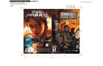
An example of a Data Parameter Dialog Box for a statistical procedure
Data Parameter Dialog Box options
Parameter Edit Boxes
Enter the number of loci, samples and pops in
each box.
Add Pop. Size by entering the required size in
the edit box above the list, then click the Add
Pops button. Add population sizes in order from
population 1 to n.
Clear Pops Use this button to clear the list of
population sizes.
Data Format
Select the format appropriate to your data.
Enter Title and Worksheet Prefix.
A Guide to GenAlEx 6.5
11 of 131
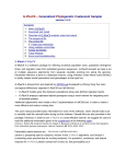
Options
The Options menu contains sub-menus for customizing the GenAlEx package.
Generic: This submenu provides options for customizing the GenAlEx dialog boxes and
output including graphs and worksheet labels.
Tip: This option may also be used to customize commonly used dialog boxes. For example, if
you mostly work with binary datasets, you can reset the default in your usual dialog boxes to
binary. After changing the dialog box options to your required settings during the course of
an analysis, return to the Generic sub-menu, and click save in the dialog box.
A Guide to GenAlEx 6.5
12 of 131
Menus: This submenu provides options for customizing the GenAlEx menu.
Tip: Teachers can use this option to hide some of the advanced options from the menu.
Install: This sub-menu installs GenAlEx so that it will launch automatically when Excel is
opened. Other versions of GenAlEx will be uninstalled by this process.
Uninstall: This sub-menu uninstalls GenAlEx, preventing it from automatically launching
when Excel is opened.
List Add-Ins: Lists the version of GenAlEx currently installed.
Check Font: Calls a dialog box stating the current standard font size set in Excel. GenAlEx is
optimized for a standard Excel font size of 10pts. This function also provides the option
of changing the standard font size to 10pt.
A Guide to GenAlEx 6.5
13 of 131
Data format for GenAlEx
Numerical Format
GenAlEx requires all data to be coded as numbers and formatted within Excel as numeric
data. Be especially careful to avoid using the text format option, and turn off all autoformatting options. Advanced options are available for processing DNA sequence data to find
polymorphisms and haplotypes and convert these to numerical format (see the ‘Raw Data
Editing’ section).
Tip: To check your numeric values are actually treated as numeric by Excel, click the
Increase or Decrease decimal buttons, under Excel’s Formatting options. If Excel is unable
to show decimals, your numbers are formatted as text not numeric.
Missing Data
Virtually all GenAlEx options handle missing data. Missing data can be particularly
problematic for pairwise distance-based analyses such as AMOVA, Mantel and spatial
autocorrelation. Therefore, a unique option for interpolating missing individual-by-individual
pairwise distances is provided. This option will insert the average genetic distances for each
population level pairwise contrast e.g. within Pop. 1, or between Pop. 1 and Pop. 2.
Nonetheless, in order to avoid excessive bias, large numbers of missing data for individualbased distance calculations should be minimized.
Codominant and Haploid missing data are coded as ‘0’.
Missing Binary data are coded as ‘-1’.
Tip: It is important to note that missing data must be coded as either 0 (Codominant and
Haploid) or -1 (Binary only). The presence of empty cells within your data, that is cells with
no values, will prevent most GenAlEx analyses from running. You can use the Data menu
option Check Raw Data to quickly locate any empty or non-numeric values in your data.
Sample Labels
If you plan to take advantage of all the features of GenAlEx, each sample must be given a
unique numerical identifier. Sample names may carry an alpha character prefix, but this must
be the same (including case) for all samples in a single dataset. In this case it is important to
know that when sorting on alphanumeric data, GenAlEx uses the Excel sort-order rules,
sorting character by character, (e.g. A11will come after A100). For ease of sorting, we
recommend that the format A001…A199 be used when using prefixes.
Note: This strict requirement for unique numerical identifiers is not essential for
running most of the population genetic analyses. However, it is required for many of the
useful data manipulation options.
Tip: If your samples are not in this format, it is possible to quickly create unique numerical
identifiers using the Replace Sample code option under the Raw Data menu in GenAlEx.
A Guide to GenAlEx 6.5
14 of 131
Data Structure
For all population-based analyses within GenAlEx, the genotypes for all the samples
belonging to a single population must be entered as a contiguous block of rows - one sample
per row. For regional-based analyses in AMOVA, all populations belonging to a region must
also be entered as a contiguous block. For TwoGener input, the genotypes of each mother and
respective offspring are entered as a contiguous block, with the mother being the first
individual of each block. Mother groupings are coded in the Column 2 (see Tutorial 6 for
more details).
Data Parameters and Labels
Data parameters and labels are crucial for telling GenAlEx how to read and analyze the data.
GenAlEx stores all parameters and labels in rows 1, 2 and 3 of the data worksheets. For raw
data, columns 1 and 2 are generally used for sample and population labels respectively;
while, actual data begins in Cell C4 of a worksheet.
Note: When analysing your data, GenAlEx only uses the data parameters to locate and
process your samples. It does not interrogate the sample or population codes in columns
1 and 2. Therefore, ensure the data parameters reflect the data format, particularly
after sorting or rearranging your samples.
Data parameters and labels may be entered in GenAlEx in several ways
1. A worksheet containing data may be manually formatted to provide appropriate
parameters.
2. The Template option in the GenAlEx menu may be used to provide parameters through a
dialog box, creating a formatted worksheet into which the data are then entered (see
section below for further instructions).
3. The Parameters option in the GenAlEx menu may be used to obtain the relevant
parameter values from an existing dataset and insert them into their appropriate location
(see section below for further instructions). This option requires that your data is
bounded by blank columns and rows.
4. On initiating an analysis, GenAlEx prompts for the relevant parameters in a dialog box.
Changing parameters in this box provides an easy way to select subsets of data for
analysis.
5. If data is imported using GenAlEx options, essential parameters and labels will be inserted
automatically, however labels for locus names may need to be entered manually.
A Guide to GenAlEx 6.5
15 of 131
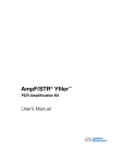
Parameter locations
Essential parameters are inserted into Row 1. They are: No Loci (cell A1); No. Samples (cell
B1); No Populations (cell C1); The size of each population (cell D1..to cell n1).
B1 : No. Samples
D1 – F1 : Size of each of 3 pops.
C1 : No. Pops.
A1 : No. Loci
A2 : optional title.
D2 – F2 : Pop. labels
Row 3 : Optional
labels, including
locus names
Col. 2 with pop. labels
in contiguous blocks.
Col. 1 with sample labels starting
in A4. Each sample has a unique
numerical number.
Codominant data as 2
columns per locus, starting
at C4.
If regional information is required, the parameter for the No. of Regions is inserted into the
cell immediate after the last population size, and the size of each region then follows in
subsequent cells (see example under codominant data below).
Data Formats
GenAlEx accepts 4 types of numerically-coded data:
1. Codominant genotypic data with 2 columns per locus.
2. Dominant (Binary), Haploid (including Haplotypes), or Sequence data coded
numerically with 1 column per locus/base.
3. Codominant and Haploid raw allele frequency data.
4. Geographic data with 2 columns for X and Y coordinates.
Tip: Examples of all GenAlEx data formats can be created via the Create menu option. This is
a useful way to explore the full range of GenAlEx options.
A Guide to GenAlEx 6.5
16 of 131
Format for codominant genotypic data
Codominant genotypic data are presented as two columns per locus as in the figure below.
Alleles may be simply numerically-coded (1, 2, 3 etc). Alternatively, and preferably for
microsatellite data, alleles may be coded as their integer size in base pairs (bp), or as the
inferred number of simple sequence repeats. These last two formats are essential for
calculation of the distance measure, Rst. There is no limit to the number of numerically-coded
alleles. Alleles coded in bp size are accepted up to a maximum allele size of 999.
Codominant alleles need not be numbered consecutively.
Example of codominant, numerically-coded data, with regional parameters.
In this example the 4 populations are split into 2 regions with Pops 1 & 2 in Region 1 and
Pops 3 & 4 in Region 2.
Example of codominant genotypic microsatellite data, with loci scored as fragment size.
A Guide to GenAlEx 6.5
17 of 131
Example of microsatellite data, with alleles coded with the inferred number of repeats.
These are the same data as the previous example, for loci of 2bp simple sequence repeats.
Format for dominant (Binary), haploid or sequence data
Dominant, haploid (including haplotypes) or sequence data are presented as a single column
per locus. Dominant data can be coded in a binary format with one column per marker.
Haploid data can be coded numerically from 1…n, or each haplotype may be represented by
multiple variable sites (columns 1 … n), with multiple states. For sequence or SNP data the
bases are numerically coded as follows: A=1, C=2, G=3, T=4, :=5; -=5, all other characters =
0. GenAlEx provides several options for the import of sequence data and auto conversion to
numbers.
Example of dominant (binary) data.
A Guide to GenAlEx 6.5
Example of sequence data, coded numerically at multiple variable sites.
Example of haplotype data, with individual haplotypes coded numerically.
These haplotypes correspond to the sequences shown in the previous example.
18 of 131
A Guide to GenAlEx 6.5
19 of 131
Format for regional data.
For regional-based analyses, all populations belonging to a single region must be entered as a
contiguous block. Region labels can be entered in columns 1 or 2 with population labels in
the alternate column. The parameters for the regional data are entered in Row 1, immediately
following the last population size.
Tip: In order to keep track of individual samples when performing regional analysis, enter
sample labels after the genetic data with a blank intervening column.
Example of data with regional parameters.
In this example the 5 populations are split into 2 regions (Cell I1) with Pops 1, 2 & 3 in
Region 1 and Pops 4 & 5 in Region 2. The first region contain 12 individuals and the second
contains seven (Cells J1 & K1).
A Guide to GenAlEx 6.5
20 of 131
Format for codominant and haploid raw allele frequency data
Codominant and haploid raw allele frequency data are presented with each locus as a
contiguous block and each allele in a separate row. The first row of each locus block must
contain the sample size of each population for that locus. Locus labels are presented in
column 1 and allele codes in column 2. The frequency of each allele is then entered for each
population in columns 3 to n.
Example of raw allele frequency data
A1 : No. Loci
B1 : No. Data Rows
C1 : No. Pops.
1st Row of a Locus Block:
Sample Size for that Pop
at that locus
Col. 1: loci
labels with
each locus in
a contiguous
block
Col 3 to n: Allele
Freq. by Pop
Col. 2:
Allele
labels
A Guide to GenAlEx 6.5
21 of 131
Format for geographic data.
For convenience, both geographic and genetic distances can be calculated in a single analysis.
Coordinates can be entered as either integer or decimal numbers.
X and Y coordinates may be read by GenAlEx from three different formats.
1. X / Y data are located in the same worksheet as the genetic data, and separated from the
genetic data by a single blank column. This format is used by GenAlEx for various
analyses, including Distance and TwoGener.
Example of geographic data after genetic data.
2. In a separate worksheet, in columns 3 and 4. In this case, the labels in columns 1 & 2 will
correspond exactly to those for the genetic data. This format is required for analyses
such as the 2D Spatial autocorrelation.
Example of geographic data in columns 3 & 4.
3. Before the genetic data, in columns 1 and 2. This format is retained to allow compatibility
with older GenAlEx datasets, but is no longer recommended.
A Guide to GenAlEx 6.5
22 of 131
Example of geographic data in columns 1 & 2.
Example of Decimal Latitude / Longitude data.
Latitude / Longitude data may contain negative values. In accordance with international
standards, latitude values should be presented first. These values are transformed
appropriately on mapping the data (Graph-> Lat/Long). Latitude / Longitude data may be
entered in any of the formats shown above.
Template
The Template option facilitates formatting a dataset for GenAlEx, by setting up a new
worksheet with the appropriate parameters and labels into which your data can be entered.
Refer to Tutorial 1, Exercise 1.9 for additional assistance with this option.
Procedure
1. With a workbook open, choose the option Template from the GenAlEx menu, and select
either Codominant , Binary or Haploid as required.
2. In the Data Parameters dialog box enter the number (#) of loci, # samples, # populations,
and, if required, # regions in the left hand side panel. These parameters are inserted into
the appropriate parameter cell on the data worksheet [D]. For codominant and haploid
data enter the max. # alleles required.
A Guide to GenAlEx 6.5
23 of 131
3. Enter the size of each pop in the edit box below ‘Pop. Size’, and add to the population list
using the add Pops. option. Use the Clear Pops. Option to clear the list. Information
regarding regions is similarly entered, if required.
4. Enter a Title and worksheet prefix for your data and click Ok. Output is to worksheet [D].
Use this template as a basis for entering your data set.
Create
The Create menu provides options to create random examples of all GenAlEx data formats,
both Genetic and Geographic. These datasets are useful for exploring the range of GenAlEx
procedures. Refer to Tutorial 1 Exercises 1.6 to 1.8 for additional assistance with this
option.
The Codominant , Codominant with phase and Haploid sub-options create data with alleles
numerically encoded. Binary data is coded as 1 / 0. The two sequence data types produce
DNA sequence data with Alpha-coding of nucleotides (i.e. A, C, G & T). The Codominant
Raw Freq. and Haploid Raw Freq. options create a data sheet containing the frequency of each
allele per locus by each population, along with a standard genotypic data sheet. The Raw
Sequence sub-option will create a data sheet with the whole length of the sequence in one
cell, whereas the Sequence sub-option will insert each nucleotide base of the sequence into a
separate cell to a max. of 254 bp in Excel 2003 or 16, 382 in Excel 2010.The sequence data is
created with a low rate of polymorphism to enable finding of haplotypes in downstream
analysis.
A Guide to GenAlEx 6.5
24 of 131
If the advanced TwoGener, Clonal or Transposed menu options are activated via the Options >Menus, the relevant Create options will also appear as submenus. The TwoGener option
creates a dataset where each offspring has at least one allele from the mother, who is
represented as the first sample in each ‘mother group’.
Geographic data can be created at the same time as genetic data and is entered in the created
worksheet after the genetic data, separated by a blank column. Alternatively, the XY and
Lat/Long sub-options will create a worksheet containing geographic coordinates in columns 3
and 4.
Tip: Create can be used to provide test datasets for the teaching environment. For
codominant data, the genotype frequency will approximate those expected under random
mating, and thus may be used to demonstrate population genetic patterns typical of random
mating.
Tip: Datasets created using this option are in correct GenAlEx format and may be used to
test unexpected GenAlEx errors. In this case, use Create to generate a dataset of identical
size to your own, and re-test the problematic procedure. If it works, the problem must lie with
your dataset.
Procedure for creating genetic data
1. With a workbook open, choose the option Create from the GenAlEx menu, and select the
genetic data type required.
2. In the Create Data Parameters dialog box enter the number (#) of loci (which equals the
number of nucleotides for sequence data), # samples, # populations, and, if required, #
regions in the left hand side panel. These parameters are inserted into the appropriate
parameter cell on the data worksheet [D]. For codominant and haploid data enter the
max. # Alleles required.
3. Indicate the population size in one of two ways. To create even sized pops ensure the Auto
Pop Size option is checked (if the sample size is not divisible by the number of pops
GenAlEx will reduce the sample size to the nearest divisible number). To create
variable sized pops, enter the size of each population in the edit box below ‘Pop. Size’,
and add to the population list using the Add Pops. option. Use the Clear Pops. option to
clear the list. Uncheck the Auto Pop Size option. Information regarding regions is
entered as for variable population sizes, if required.
4. To create a list of geographic coordinates after the genetic data, check the XY Coords
option.
5. Enter a Title and worksheet prefix for your data and click Ok. Output of genotype data is to
worksheet [D], while raw frequencies created by the Codominant Raw Freq. and Haploid Raw
Freq options are output to worksheet [RAFP].
A Guide to GenAlEx 6.5
25 of 131
Procedure for creating geographic data
1. With a workbook open, choose the option Create from the GenAlEx menu, and select
either the XY and Lat/Long sub-options.
2. In the GenAlEx input dialog box enter the number (#) of coordinates (samples) required
and click Ok. Output is to worksheet [XY].
Parameters
The Parameters option provides a quick means to obtain the necessary GenAlEx parameters
from a pre-existing dataset, and insert them in their correct location. Unless otherwise
indicated data must be in standard GenAlEx format, with data labels in column 1 and 2, and
data starting in cell C4. The dataset needs to be bounded by empty rows and columns, as
GenAlEx uses empty cells to define the limits of the data. All samples per population and
region must have the same case sensitive population and region labels respectively, and be in
a contiguous block. For each menu sub-option, GenAlEx will interrogate the chosen
column(s) and insert the corresponding parameters in the correct locations. Refer to Tutorial
1, Exercises 1.10 for additional assistance with this option.
All for Codom: When population labels are entered in column 2 this option correctly inserts
loci, sample and population parameters for codominant data sets in standard GenAlEx
format.
A Guide to GenAlEx 6.5
26 of 131
All for Haploid: When population labels are entered in column 2 this option correctly inserts
loci, sample and population parameters for haploid data sets in standard GenAlEx
format.
All from Raw Freq.: This option will insert the loci, sample and population parameters when
the data is in the standard GenAlEx raw frequency format (see the ‘Data Formats’
section).
Pops from Col 2: When population labels are entered in column 2 this option correctly inserts
sample and population parameters.
Pops from Col1: When the population labels are entered in column 1this option correctly
inserts sample and population parameters.
Samples from Col1: When sample labels are in column 1 this option correctly inserts sample
parameters. This option assumes the data only contains one population and inserts
population parameters accordingly.
Loci: Inserts the correct number of loci when each locus is entered as a single column (i.e
when it is Haploid, Dominant (Binary) or sequence data).
Codominant Loci: Inserts the correct number of loci when each locus is entered as two
adjacent columns (i.e one column for each codominant allele).
Pops + Regions from Col1 + 2: When population and region labels are in columns 1 and 2
respectively, this option correctly inserts the sample, population and region parameters.
Regions + Pops from Col1 + 2: When region and population labels are in columns 1 and 2
respectively, this option correctly inserts the sample, population and region parameters.
Pops from Range: In the GenAlEx Input dialog box select the range that contains the
population labels in contiguous blocks in a single column. This option will then insert the
sample and population parameters.
Pops + Regions from Range: In the GenAlEx Input dialog box select the range that contains
two columns with the population labels in the first column and the region labels in the
second. This option will then insert the sample, population and region parameters.
Note: If the sample number has not been entered into B1 or the number entered does
not equal the number of rows selected then GenAlEx will warn you that the range does
not equal the number of samples. If you proceed then GenAlEx will determine the
number of samples from the selected range.
Regions + Pops from Range: In the GenAlEx Input dialog box select the range that contains
two columns with the region labels in the first column and the population labels in the
second. This option will then insert the sample, population and region parameters.
Insert Header Rows and Params: Inserts two rows at the top of an active worksheet. If the data
is arranged with the first row containing column labels, then this option will also
correctly insert the sample parameters. This option assumes the data only contains one
population and inserts population parameters accordingly.
A Guide to GenAlEx 6.5
27 of 131
Data
The Data menu option offers several commands for quickly manipulating your dataset.
Sort on Sample (Col1): Sorts the entire dataset on column 1(normally containing the sample
labels), according to the Excel sort-order rules (see the ‘Sample Labels’ section). Data
must be in appropriate GenAlEx format (including parameters). The sample and
population parameters are automatically inserted after the data is sorted; GenAlEx
assumes population codes are in column two.
Sort on Pop (Col2): Sorts the entire dataset on column 2 (normally containing the population
labels), according to the Excel sort-order rules (see the ‘Sample Labels’ section). Data
must be in appropriate GenAlEx format (including parameters). The sample and
population parameters are automatically inserted after the data is sorted; GenAlEx
assumes population codes are in column two.
Sort on Sample + Pop (Col1+2): First sorts the entire dataset on column 1 (normally containing
the sample labels), then sorts the data within each column 1 (sample) group on column
2 (normally containing the population labels). Data must be in appropriate GenAlEx
format (including parameters). The sample and population parameters are automatically
inserted after the data is sorted; GenAlEx assumes population codes are in column two.
Sort on Pop + Sample (Col2+1): First sorts the entire dataset on column 2 (normally containing
the population labels), then sorts the data within each column 2 (population) group on
column 1 (normally containing the sample labels). Data must be in appropriate
GenAlEx format (including parameters). The sample and population parameters are
automatically inserted after the data is sorted; GenAlEx assumes population codes are
in column two.
Select Data Rows: Enables rapid selection of all data rows. This is useful for subsequent
sorting on any column using the Excel Sort option, in the Data menu.
Select Data Rows + Labels: Enables rapid selection of all data rows, and labels (Row 3). This
is useful for subsequent sorting on any column using the Excel Sort option, in the Data
menu.
Split by Pop: Splits data from multiple populations contained in a single dataset. Each
individual population dataset is moved to a separate worksheet, labeled with the name
of the population. Data must be in appropriate GenAlEx format (including parameters).
List Worksheets [WS List]: Outputs a list of all worksheets in the active workbook together
with their position in the workbook and the contents of Cells A1, B1, A2, B2 and C2.
List Data Worksheets [DWS Lists]: Outputs a list of all GenAlEx formatted data worksheets in
the active workbook together with their position in the workbook and their parameters.
List Results Worksheets: Outputs a list of all GenAlEx results worksheets in the active
workbook together with their position in the workbook, their title and source data sheet.
Sort Worksheets: This option sorts all work sheets in a workbook alphabetically.
Sort Selected Worksheets: Select the desired worksheets for sorting, and then select this
option. This option sorts the selected worksheets alphabetically and then places them in
positions 1 to n in the workbook.
A Guide to GenAlEx 6.5
28 of 131
Count list from Range: Identifies the number of occurrences of each unique alphanumeric
value within a specified range. When prompted by the GenAlEx Input dialog box
indicate the desired range. The Output is to a specified location within the active
worksheet. When prompted by the GenAlEx Input dialog box indicate the desired
location for the first cell of the output table.
Comments from Range: Lists all Excel comment bubbles and the corresponding cell value for
cells within a specified range. The output is to a specified location within the active
worksheet. When prompted by the GenAlEx Input dialog box indicate the desired
range and the location of the first cell of the output.
Row and Column No.: Returns the alphanumeric row and column value of the active cell in a
dialog box.
Check Raw Data: Runs a check of genetic data in GenAlEx format for the given parameters,
and provides a list of any data cells with empty or non-numeric values. Before you can
run any genetic analysis, empty values must be replaced by the appropriate missing
value code (0 for all data types except binary, -1 for binary data), and non numeric
values must be replaced by numeric values.
Check Raw Data: Runs a check of distance matrices in GenAlEx format for the given
parameters, and provides a list of any data cells with empty or non-numeric values.
Before you can run any genetic analysis, empty values must be replaced by the
appropriate missing value code (0 for all data types except binary, -1 for binary data),
and non numeric values must be replaced by numeric values.
A Guide to GenAlEx 6.5
29 of 131
Frequency Based Statistical Procedures
Frequency
This menu option provides a range of summary statistics for codominant, haploid and
dominant (Binary) data. Tutorial 1, Exercises 1.2 to 1.5 provide a guide to calculating many
of these statistics by hand. Tutorial 1, Exercises 1.11 and 1.12 provide further assistance
with generating these summary statistics using GenAlEx.
Procedure
1. Choose the option Frequency from the GenAlEx menu.
2. Enter all appropriate information in the Allele Frequency Data Parameters dialog box
and click Ok.
3. Select the frequency options required from the Frequency Options dialog box (option
availability depends on data type), for information about these options see below. See
below for the output sheet names.
Codominant Frequency Options
A Guide to GenAlEx 6.5
30 of 131
Frequency by Pop [AFP]: Outputs allele frequencies at each locus by population.
Graph All Loci [AGL]: Provides a single graph of locus by locus allele frequency
data. For large datasets this output can take some time, and it may be preferable to skip
this option
Graph by Locus [AGF]: Provides individual locus graphs of Allele Frequency Data.
For large datasets this output can take some time, and it may be preferable to skip this
option
Graph by Pop for each Locus[AGP]: Provides individual worksheets for each locus.
Each worksheet provides an individual pie chart of allele frequencies for each
population.
Frequency by Locus [AFL]: Outputs allele frequencies in each population with loci in
columns. For microsatellite datasets (with alleles coded by size in base pairs), this
option produces a table with the number of rows equal to the number of distinct allele
sizes across the range encountered in the whole dataset. For such datasets, often with
certain allele sizes missing, output can take some time.
Tip: The tabled data provide a good visual indication of size distribution of alleles, and
size overlap between loci, and can be a useful tool for planning the multiplexing of
different loci. The Allele list is an alternative for this.
Het, Fstat & Poly by Pop [HFP]: Outputs for each population in rows: number of samples
(N), the number of alleles (Na), the effective number of alleles (Ne), the information
index (I), the observed (Ho), expected (He) and unbiased expected heterozygosity (uHe),
and Fixation index (F). This option also outputs the mean over loci and the standard
error of each statistic per population along with the grand mean. It also outputs the F
statistics (Fis,Fst and Fit) along with the number of effective migrants (Nm) for each
locus and the mean across loci. The percentage of polymorphic loci is provided per
population. This is the standard format for most primer note publications.
Het, Fstat & Poly by Locus [HFL]: Outputs the same information as the previous option,
but with loci in columns not rows.
Allelic Patterns [APT]: Summarizes the mean and standard errors across loci for each
population of the following statistics: Number of alleles (Na), Na with frequency >5%,
effective number of alleles (Ne), information index (I), Number of private alleles,
Number of Locally Common alleles (frequency >=5%) found in <=25% and <=50% of
populations, expected heterozygosity (He) and unbiased expected heterozygosity (uHe).
Graph Pattern [APT]: Provides graphical output of the above information.
Allele list [ALI]: Tallies for each locus the occurrence of all distinct allele sizes across the
range encountered in the whole dataset.
Tip: This is a useful tool for planning the multiplexing of different loci.
Private alleles list [PAS] & [PAL]: Outputs to sheet [PAS] a list of the private alleles by
population, and outputs to sheet [PAL] a list of the samples containing one or more
private alleles. This is in standard GenAlEx format for further analyses if required.
Nei Distance: Outputs the pairwise population Nei’s Genetic Distance and Nei’s Genetic
Identity.
Nei Unbiased Distance: Outputs the pairwise Nei’s Unbiased Genetic Distance and Nei’s
Genetic Identity between populations.
A Guide to GenAlEx 6.5
31 of 131
Pairwise Fst : Outputs the pairwise Fst values between populations.
Output Pairwise Matrix: Outputs pairwise population statistics as a triangular Matrix.
Output is to worksheet [NeiP] for Nei’s Genetic Distance, to [uNeiP] for Nei’s
Unbiased Genetic Distance and to [FstP] for Pairwise Fst. This is in GenAlEx format
for further analyses if required.
Output Labeled Pairwise Matrix: Outputs pairwise population statistics as a labeled
triangular Matrix. Output is to worksheet [NeiL] for Nei’s Genetic Distance, to [uNeiL]
for Nei’s Unbiased Genetic Distance and to [FstL] for Pairwise Fst.
Output Pairwise Matrix as Table: Outputs pairwise population statistics as a table.
Output is to worksheet [NeiT] for Nei’s Genetic Distance, to [uNeiT] for Nei’s
Unbiased Genetic Distance and to [FstT] for Pairwise Fst.
Step by Step: When the appropriate Multiple Pop, Allelic Patterns or Allele Frequency and
Heterozygosity options are ticked this option outputs allele counts to worksheets [AFP]
and [AFL]; Ht, He and Ho to worksheets [HFP] and [HFL]; per locus statistics for each
population to worksheet [APT]; and the step by step calculations of Nei’s Genetic
Distance and Identity to worksheet [SbySN].
Binary (Diploid) frequency options
A Guide to GenAlEx 6.5
32 of 131
Frequency & Heterozygosity by Pop [BAFP]: Outputs in rows band frequency, (p & q),
number of samples (N), number of bands (Na), the effective number of alleles (Ne), the
information index (I), expected heterozygosity (He) and unbiased expected
heterozygosity (uHe) for each locus per population, the mean over loci per population
and the grand mean. At the end of the output, the % of polymorphic loci, P, is output
for each population.
Frequency & Heterozygosity by Locus [BAFL]: Outputs the same information as the
previous option, but with loci in columns not rows.
Allelic Patterns [BAPT]: Summarizes for each population the following statistics: Number
of bands, Number of bands with frequency >=5%, Number of private bands, Number of
Locally Common bands (frequency >=5%)found in <=25% and <=50% of populations,
mean expected heterozygosity (He) and unbiased expected heterozygosity (uHe) along
with their standard errors.
Graph Pattern [BAPT]: Provides graphical output of the above information.
Nei Distance: Outputs the pairwise population Nei’s Genetic Distance and Nei’s Genetic
Identity.
Nei Unbiased Distance: Outputs the pairwise population Nei’s Unbiased Genetic Distance
and Nei’s Genetic Identity.
Output Pairwise Matrix: Outputs pairwise population statistics as a triangular Matrix.
Output is to worksheet [NeiP] for Nei’s Genetic Distance and [uNeiP] for Nei’s
Unbiased Genetic Distance. This is in GenAlEx format for further analyses if required.
Output Labeled Pairwise Matrix: Outputs pairwise population statistics as a labeled
triangular Matrix. Output is to worksheet [NeiL] for Nei’s Genetic Distance and to
[uNeiL] for Nei’s Unbiased Genetic Distance.
Output Pairwise Matrix as Table: Outputs pairwise population statistics as a table.
Output is to worksheet [NeiT] for Nei’s Genetic Distance and to [uNeiT] for Nei’s
Unbiased Genetic Distance.
Step by Step: Outputs step by step calculations of Nei’s Genetic Distance and Identity to
worksheet [SbySN], when the Nei Distance option is ticked.
A Guide to GenAlEx 6.5
33 of 131
Binary (Haploid) frequency options
Frequency & Heterozygosity by Pop [BAFP]: Outputs in rows the band frequency, (p &
q), number of samples (N), number of bands (Na), the information index (I), diversity
(h) and unbiased diversity (uh) for each locus per population, the mean over loci per
population and the grand mean. At the end of the output, the % of polymorphic loci, P,
is output for each population.
Frequency & Heterozygosity by Locus [BAFL]: Outputs the same information as the
previous option, but with loci in columns not rows.
Allelic Patterns [BAPT]: Summarizes for each population the following statistics: Number
of bands, Number of bands with frequency >=5%, Number of private bands, Number of
Locally Common bands (frequency >=5%) found in <=25% and <=50% of populations,
mean diversity (h) and unbiased diversity (uh) along with their standard errors.
Graph Pattern [BAPT]: Provides graphical output of the above information.
Nei Distance: Outputs the pairwise Nei’s Genetic Distance and Nei’s Genetic Identity
between populations.
Nei Unbiased Distance: Outputs the pairwise Nei’s Unbiased Genetic Distance and Nei’s
Genetic Identity between populations.
Output Pairwise Matrix: Outputs pairwise population statistics as a triangular matrix.
Output is to worksheet [NeiP] for Nei’s Genetic Distance and [uNeiP] for Nei’s
Unbiased Genetic Distance. The output is in GenAlEx format for further analyses if
required.
Output Labeled Pairwise Matrix: Outputs pairwise population statistics as a labeled
triangular matrix. Output is to worksheet [NeiL] for Nei’s Genetic Distance and to
[uNeiL] for Nei’s Unbiased Genetic Distance.
Output Pairwise Matrix as Table: Outputs pairwise population statistics a table.
Output is to worksheet NeiT for Nei’s Genetic Distance and to uNeiT for Nei’s
Unbiased Genetic Distance.
Step by Step: Outputs step by step calculations of Nei’s Genetic Distance and Identity to
worksheet [SbySN], when the Nei Distance option is ticked.
A Guide to GenAlEx 6.5
34 of 131
Haploid frequency options
Frequency by Pop [HAFP]: Outputs frequencies of alleles at each locus for each
population.
Graph All Loci [HAGL]: Provides graphical output of the above information. For
large datasets output can take some time, and it may be preferable to skip this option.
Graph by Locus [HAGF]: Provides individual locus graphs of Allele Frequency Data.
For large datasets this output can take some time, and it may be preferable to skip this
option.
Graph by Pop for each Locus [HAGP]: Provides individual worksheets for each
locus. Each worksheet provides an individual pie chart of allele frequencies for each
population.
Frequency by Locus [HAFL]: Outputs allele frequencies in each population with loci in
columns.
A Guide to GenAlEx 6.5
35 of 131
Haploid Diversity by Pop [HDP]: Outputs in rows the number of samples (N), number of
alleles (Na), the effective number of alleles (Ne), the information index (I), diversity (h)
and unbiased diversity (uh) for each locus per population, the mean over loci per
population and the grand mean. At the end of the output, the % of polymorphic loci, P,
is output for each population.
Haploid diversity by Locus [HDL]: Outputs the same information as the previous option,
but with loci in columns not rows.
Allelic Patterns [HAPT]: Summarizes the mean and standard errors across loci by
population for the following statistics: number of alleles (Na), Na with frequency
>=5%, effective number of alleles (Ne), Number of Locally Common alleles (frequency
>=5%) found in <=25% and <=50% of populations, haploid diversity (h) and unbiased
diversity (uh).
Graph Pattern [HAPT]: Provides graphical output of the above information.
Haploid disequilibrium [HDE] & [FDHDE]: Outputs the haploid disequilibrium analysis
and the results of the randomization test of significance to sheet [HDE]. Also outputs
the frequency distribution indicating were the data observed variance (Vo) lies within
the randomly generated observed variances to sheet [FDHDE]. When prompted by the
GenAlEx Input dialog box specify the desired number of randomizations for testing
the significance of haploid disequilibrium (0, 99, 999). This option only applies with a
single population.
Input is Haplotypes: Checking this option when a haplotype is coded as a single locus
ensures that the output is annotated for haplotype data. This option is only available
with single locus data.
Allele List [HALI]: Tallies the occurrence of alleles for each locus over the whole dataset.
This is a useful tool for planning the multiplexing of different loci.
Private Alleles List [PAS] & [PAL]: Outputs to sheet [PAS] a list of the private alleles by
population, and to output sheet [PAL] a list of the samples containing one or more
private alleles. This output is in standard GenAlEx format for further analyses if
required.
Nei Distance: Outputs the pairwise Nei’s Genetic Distance and Nei’s Genetic Identity
between populations.
Nei Unbiased Distance: Outputs the pairwise Nei’s Unbiased Genetic Distance and Nei’s
Genetic Identity between populations.
Output Pairwise Matrix: Outputs pairwise population statistics as a triangular matrix.
Output is to worksheet [NeiP] for Nei’s Genetic Distance and [UNeiP] for Nei’s
Unbiased Genetic Distance. This output is in GenAlEx format for further analyses if
required.
Output Labeled Pairwise Matrix: Outputs pairwise population statistics as a labeled
triangular matrix. Output is to worksheet [NeiL] for Nei’s Genetic Distance and to
[UNeiL] for Nei’s Unbiased Genetic Distance.
Output Pairwise Matrix as Table: Outputs pairwise population statistics a table.
Output is to worksheet NeiT for Nei’s Genetic Distance and to UNeiT for Nei’s
Unbiased Genetic Distance.
A Guide to GenAlEx 6.5
36 of 131
Step by Step: When the appropriate Multiple Pop, Allelic Patterns or Allele Frequency
options are ticked this option outputs allele counts to worksheet [HAFP] and [HAFL];
per locus statistics for each population to worksheet [HAPT]; and the step by step
calculations of Nei’s Genetic Distance and Identity to worksheet [SbySN].
A Guide to GenAlEx 6.5
37 of 131
Disquil
This menu contains two sub-menus. The HWE sub-menu tests each locus by population for
despatchers from the expected genotype frequencies under Hardy-Weinburg equilibrium. The
Paired Biallelic LD sub-menu tests for linkage disequilibrium between loci for each
population.
HWE
The Hardy-Weinberg option only applies to codominant data.
Note: The Chi-squared test of Hardy-Weinberg equilibrium offered in GenAlEx is
primarily for teaching and data exploration. An alternative statistical test for assessing
an overall departure from random mating is provided in GenAlEx via the AMOVA
framework. Other programs provide Exact Tests that are recommended for research
purposes. GenAlEx offers data export to these programs. See the GenAlEx 6.5
Appendix 1 for more details.
Procedure
1. Choose the option HWE option from the GenAlEx menu.
2. Enter all appropriate information in the HWE Data Parameters dialog box, click Ok.
3. In the subsequent Hardy-Weinberg Options dialog box choose required options (see
below), click Ok. See options below for the output sheet names.
Hardy-Weinberg options
Observed vs. Expected Values [HW]: Outputs the observed and expected frequencies of
each genotype, and the Chi-Square test for each locus in each population.
Graph Obs. v Exp. [HW]: Outputs graphs for above genotype data.
Summary [HWS]: Provides a summary of the Chi-Squared statistic, degrees of freedom, and
probability for each locus in each population.
Step by step [HW]: Shows step by step calculations for the Chi-Squared test.
A Guide to GenAlEx 6.5
38 of 131
Paired Biallelic LD
The Paired Biallelic Linkage Disequilibrium option only applies to codominant biallelic data
with the two alleles at each locus coded as ‘1’ and ‘2’.
Procedure
1. Choose the Paired Biallelic LD sub-menu option from the Disequil menu.
2. Enter all appropriate information in the Paired Linkage Disequilibrium Data
Parameters dialog box, click Ok.
3. In the subsequent Paired Linkage Disequilibrium Options dialog box choose the
required options (see below), click Ok. See options below for the output sheet names.
Pairwise Linkage Disequilibrium options
Biallelic-Known Phase: Select this option if for each locus and individual every allele can
be designated as of paternal or maternal origin. For data of known phase, the maternal
gamete must be entered in the first column of each loci with the paternal gamete
entered in the second column (or vice versa).
Biallelic-Unknown Phase: Select this option if the origin (maternal or paternal) of the alleles
is unknown.
Full Analysis: For data with known phase, this option outputs separate matrices of linkage
disequilibrium, gene frequency correlation, Chi-squared statistics and probabilities for
each locus pair by population to worksheet [LDK]. For data with unknown phase, this
option outputs for each locus pair by population a table of disequilibrium statistics for
both possible states (possible maternal/paternal gametes). Output is to worksheet
[LDU].
A Guide to GenAlEx 6.5
39 of 131
Summary Table: Outputs a summary table of disequilibrium statistics pairwise between
loci. For data of known phase, the estimated genetic linkage disequilibrium,
standardized D, correlation of gene frequencies, Chi-squared statistic and
corresponding probability are output to worksheet [LDKS]. For data of unknown phase,
Disequilibrium estimates and chi-squared statistics both assuming and not assuming
Hardy-Weinberg equilibrium are output to worksheet [LDUS].
Graph D and r values: Outputs separate graphs for the disequilibrium estimates and
gene frequency correlations by each loci pair to worksheet [LDKS] or [LDUS]. If this
option is selected then GenAlEx assumes Summary Table has been checked.
Step by Step: For data of known phase, this option outputs allele and haplotype counts along
with observed and expected haplotype frequencies to worksheet [LDK]. For data of
unknown phase, this option outputs allele and genotype counts along with allele
frequencies and the maximum likelihood estimated frequency of gamete 11 to
worksheet [LDU]. If this option is selected then GenAlEx assumes Full Analysis has
been checked.
Note: If neither Full Analysis nor Summary Table has been checked then GenAlEx will
default to Summary Table (without graphs).
A Guide to GenAlEx 6.5
40 of 131
G-Statistics
This menu option calculates a range of recently developed frequency based population
structure estimators for codominant data. These measures include Gst, Nei’s standardized
Gst, Hedrick’s standardized Gst, Hedrick’s further standardized Gst for small number of
populations and Jost’s estimate of differentiation. These estimators can be calculated across
populations or pairwise. Fst can also be calculated by this menu to facilitate comparison with
the newly developed statistics. Significance tests of the calculated measures, via permutation,
are available for genotypic data. For further information on these recently developed statistics
including formulas refer to GenAlEx 6.5 Appendix 1.
Procedure
1. Choose the G-Statistics sub-menu from the GenAlEx menu.
2. Ensure the data parameters are correct and select the appropriate data type in the GStatistics Data Parameters dialog box, click Ok. If the input is raw frequency data, then a
subsequent Raw Frequency Parameters dialog box will follow. Ensure the data
parameters are correct, click Ok.
3. In the G-Statistics Options dialog box choose the desired options (see below), click Ok.
See options below for the output sheet names.
A Guide to GenAlEx 6.5
41 of 131
G-Statistics Options
Output Options:
# Permutations: Enter the number of permutations desired for calculating the probabilities
for the G-statistics over all populations. Permutation tests are only available for
codominant genotypic data, not raw allele frequency data.
# Bootstraps: Enter the number of bootstraps desired for calculating standard errors and
confidence intervals. Bootstraps only apply when more than 5 loci are being analyzed.
Full Analysis[Gst]: Outputs the following statistics combined over all populations in table
format for each locus and over all loci, along with standard errors and confidence
intervals: total number of samples (N), the average number of alleles (Na), the overall
effective number of alleles (Ne), the average effective number of alleles (cNe), the
mean observed (Ho) and expected heterozygosity (Hs), the total expected
heterozygosity (Ht), the corrected mean (cHs) and total expected heterozygosity (cHt),
the maximum Gst (GstM), Fis, Fst, Gis, Gst, Nei’s standardized Gst (G’stN), Hedrick’s
standardized Gst (G’stH), Hedrick’s further standardized Gst for small number of
populations (G’’st) and Jost’s estimate of differentiation (Dest). In the case of
codominant genotypic data this option also outputs a table listing the probabilities for
the G-statistics.
Summary [GstG]: Outputs the following statistics combined over all populations in table
format for each locus and over all loci, along with standard errors and confidence
intervals: Gst, Nei’s standardized Gst (G’stN), Hedrick’s standardized Gst (G’stH),
Hedrick’s further standardized Gst for small number of populations (G’’st) and Jost’s
A Guide to GenAlEx 6.5
42 of 131
estimate of differentiation (Dest). In the case of codominant genotypic data this option
also outputs a table listing the probabilities for the output G-statistics.
Graph G-Statistics: Outputs a graph of the G-statistic values by each locus and overall
to sheet [GstG].
Summary by Locus[GstS]: Outputs the following statistics combined over all populations in
table format with loci in columns: Fis, Fst, Gis, Gst, Gst, Nei’s standardized Gst
(G’stN), Hedrick’s standardized Gst (G’stH), Hedrick’s further standardized Gst for
small number of populations (G’’st) and Jost’s estimate of differentiation (Dest). In the
case of codominant genotypic data this option also outputs a table listing the
probabilities for the output statistics.
Step by Step: This option is currently not implemented.
Freq. Dist.: This option is currently not implemented.
Pm Values [GstPm]: Outputs the statistics listed under Full Analysis for each permutation.
This option is only available for codominant genotypic data, not raw allele frequency
data.
Pairwise Options:
For the pairwise population options the suffixes of the output worksheets represent the
combination of options selected. For example, if Pairwise Output for Total Only [Tot],
Output Pairwise Matrices[P] and For: Fst [Fst] are selected then the output worksheet
suffix would be [Tot FstP].
# Permutations: Enter the number of permutations desired for calculating the probabilities
for the pairwise G-statistics. Permutation tests are only available for codominant
genotypic data, not raw allele frequency data.
Pairwise Output for Total Only [Tot]: Outputs a pairwise population matrix with the
selected statistic combined across all loci below the diagonal (see below). For
codominant genotypic data pairwise probabilities for the selected statistic are entered
above the diagonal.
Pairwise Output for Each Locus: In addition to the output of a pairwise population matrix
with the selected statistic combined across all loci, a pairwise population matrix of the
selected static is output for each locus separately to a different appropriately named
worksheet e.g [Locus1].
Output Pairwise Matrices[P]:Outputs a pairwise population matrix for each selected
statistic in standard GenAlEx format.
Output Labeled Matrices[L]: Outputs a labeled pairwise population matrix for each
selected statistic.
Output Pairwise Matrices as Table: Outputs a pairwise population matrix as a table for
each selected statistic.
For: Select the desired statistics to be output in pairwise population matrices from the
following: Fst [Fst]; Gst [Gst]; Nei’s standardized Gst = G’st (Nei) [GstN]; Hedrick’s
standardized Gst = G’st (Hed) [GstH]; Hedrick’s further standardized Gst for small
number of populations = G’’st [GstC]; and Jost’s estimate of differentiation = Dest
[Dest].
A Guide to GenAlEx 6.5
43 of 131
Shannon
Shannon’s diversity index for information theory (Shannon 1948) has been widely employed
in ecology but has been less widely used in population genetics. In a recent series of studies,
Sherwin et al. (2006) and Rossetto et al. (2008) have shown both by computer simulation and
for real data sets that Shannon’s Indices offer some ideal statistical properties for measuring
biological information across multiple scales from genes to landscapes. In particular, the
capacity to apply the indices at multiple scales is unique among the commonly employed
population statistics. In GenAlEx Shannon indices can be calculated for codominant or
haploid data via the Shannon menu options. For further assistance with calculating Shannon
indices by hand and in GenAlEx refer to Tutorial 1, Exercises 1.13 and 1. 15. For formulas
refer to GenAlEx 6.5 Appendix 1. Additional background on the application of Shannon
indices to population genetics is also provided in the Appendix to Tutorial 1 written by WB
Sherwin.
Pairwise Pops
The Pairwise Pops sub-menu computes Shannon’s mutual information index S HUA between
populations, a pairwise measure of differentiation. This option also provides a convenient
chi-square based statistical test for allele frequency differences between each pairwise
combination of populations through the conversion of SHUA to the log-likelihood contingency
test G statistic. This option only applies to codominant and haploid data.
Procedure
1. Activate the worksheet containing your dataset in standard GenAlEx format. Choose the
option Shannon from the GenAlEx menu, and then select the submenu option Pairwise
Pops.
2. Ensure the locus and sample parameters are correct in the Shannon Pairwise Pops Data
Parameters dialog box.
3. Enter Title and Worksheet Prefix then click Ok.
A Guide to GenAlEx 6.5
44 of 131
4. In the subsequent Pairwise Pops Shannon Analysis Options dialog box, select the
options required (see below). Then Click Ok. Summary of the Shannon analysis,
including Shannon’s mutual information index SHUA, G statistic and Chi significance
test, over loci for all pairwise population combinations is output to worksheet [SH].
Pairwise Pops Shannon Analysis Options
Single Locus: Outputs Shannon’s allelic diversity index SHA for each locus by Population to
worksheet [sHa].
Full Analysis: Check this option to output the summary of Shannon analysis over loci for all
pairwise Population Combinations to worksheet [SH]. Note that the summary table will
reflect the pairwise options selected below. For example, if you select Output for Total
Only, the summary table will only show the Mean over Loci.
Output for Total Only: Outputs mean values for Shannon’s indices over loci for all pairwise
population combinations.
A Guide to GenAlEx 6.5
45 of 131
Output for Each Locus: In addition to the mean values for the Shannon’s indices, this
option outputs the summary of the Shannon analysis for each loci to worksheet [SH].
When one of the output pairwise matrices options is selected, this option also outputs
pairwise matrices for each locus to separate appropriately named worksheets e.g [Locus
4 SHuaP].
Output Freq. [AFPT]: Outputs allele frequencies and samples sizes by locus for each
population.
Step by Step: Outputs step by step calculations of Shannon’s mutual information index SHUA
for all pairwise population combinations at each loci to separate appropriately named
worksheets e.g [Locus2 SHSbyS].
Outputs Pairwise Matrices: Outputs a series of matrices containing the pairwise Shannon
indices (SHA, SHU , SHUA), and estimated number of migrants between populations to
sheet [SHaP].
Output Labeled Pairwise Matrices: Outputs labeled versions of the above described
pairwise matrices to sheet [SHaL].
Output Pairwise Matrices as Table: Outputs the above described pairwise matrices as
tables to sheet [SHaT].
Set sHua to Zero when Less Than: Select a cut off value below which sHua values will be
converted to zero. This option prevents anomalous estimates of migrants between
populations (Nm) due to very small sHua values. The default value is 0.0001.
Log Base Options:
Select the log base for calculating the Shannon diversity indices. Log base 2 is recommended
by Sherwin et al. (2006) as it translates to heterozygosity. However, the natural Log is
commonly used in ecology and may be useful for comparison between different levels
of diversity. Log base 10 is also available. The value of the Shannon indices will
change with the base selected; however, the estimated number of migrants is
unaffected.
Optional Estimated Pop Sizes Data:
The effective population size of each population can be used in the calculation of the
Shannon Indices and in the estimation of the effective number of migrants. To do so,
ensure Worksheet is ticked and select the appropriate worksheet from the dropdown
list. The worksheet containing the effective population size data must be in GenAlEx
format (with parameter and data starting in row 4) with population codes in column 2
and estimated effective population sizes in column 3. If this option is not required
select None. Where possible this option is recommended for accurate estimation of
effective migrants when effective population sizes are less than 500 for diploids or
1000 for haploids.
Note: If the estimated population sizes option is selected G-analysis is suppressed.
A Guide to GenAlEx 6.5
46 of 131
Example of format for effective population size data:
Partition
The Partition sub-menu partitions genetic diversity into three levels (e.g. within populations,
among populations and among regions) using Shannon indices. In addition to calculating
Shannon’s mutual information index this menu option derives a standardized measure of
diversity that is bounded by zero and one, allowing easy comparison between studies. This
option also provides a random permutation test for statistical significance in place of the Gtest offered under the Shannon Pairwise option. For research purposes, statistical testing by
random permutation is recommended because there are reports that the log-likelihood G-test
may exhibit high type I error rates (false rejection of the null hypothesis). This option only
applies to codominant and haploid data.
Procedure
1. Activate the worksheet containing your dataset in standard GenAlEx format. Choose the
option Shannon from the GenAlEx menu, and then select the submenu option Partition.
2. Ensure the parameters, including the population and region sizes, are correct in the
Shannon Partition Data Parameters dialog box.
3. Select the appropriate input data type. Enter Title and Worksheet Prefix then click Ok.
A Guide to GenAlEx 6.5
47 of 131
4. In the subsequent Shannon Partition Analysis Options dialog box, select the options
required (see below). Then Click Ok.
Shannon Partition Analysis Options
Single Locus [SHa]: Outputs Shannon’s information index (SHa) by locus for each
population, region and in total.
Full Analysis: Check this option to output locus-by-locus Shannon partitions within and
among populations and regions (if available) to worksheet [Locus1 SHT] etc. Note that
unlike the Pairwise Pops submenu option the summary sheet [SH] is always output.
However, the summary table will reflect the pairwise options selected below. For
example, if you select Output for Total Only, the summary table will only show the
Mean over Loci.
Output for Total Only: Outputs mean values for the Shannon indices over loci for all
pairwise population combinations.
Output for Each Locus: In addition to the mean values for the Shannon indices this option
also outputs pairwise matrices for each locus to separate appropriately named
worksheets e.g [Locus 4 SHuaP].
A Guide to GenAlEx 6.5
48 of 131
Output Pairwise Matrices [SHuaP]: Outputs the pairwise Shannon Mutual information
index SHUA.
Output Labeled Pairwise Matrices [SHuaL]: Outputs labeled versions of the pairwise
matrices described above.
Set sHua to Zero when Less Than: Select a cut off value below which sHua values will be
converted to zero. This option prevents anomalous estimates of migrants between
populations (Nm) due to very small sHua values. The default value is 0.0001.
Output Freq. [AFPT]: Outputs allele frequencies and sample sizes by locus for each
population, region and in total.
Log Base Options:
Select the log base for calculating the Shannon diversity indices. Sherwin et al. (2006)
recommended Log base 2 as it translates to heterozygosity. However, the natural Log is
commonly used in ecology and may be useful for comparison between different levels
of diversity. Log base 10 is also available. The value of the Shannon indices will
change with the base selected; however, the standardized diversities alpha, beta,
gamma, delta and omega are not changed.
5. In the Shannon Permute Options dialog box, indicate the number of permutations
required and select the desired output (see below). Then Click Ok. The Shannon
statistics partitioned by population, region and total are output separately for each locus
to an appropriately named worksheet e.g. [Locus1 SHT]. A summary of the Shannon
analysis over loci is also output to worksheet [SH].
A Guide to GenAlEx 6.5
49 of 131
Shannon Permute Options
Total Data Options:
#Permutations: Enter the number of permutations required to test for significance. Note: For
large data sets, permutation may take some time. Watch the status bar for progress. For
publication purposes the number of permutations should be set to 999 or 9999.
Standard permute: Shuffles individuals between populations and regions.
Specialized permute: Only shuffles individuals within regions when estimating the
probability for diversity among populations within regions. When estimating the
probability for diversity among regions, whole populations are shuffled among regions.
Permute Values [Pm SH]: Outputs from each standard permutation the Shannon indices and
standardized diversity for within populations, between populations and among regions.
Freq. Dist. For SH Among Pops: Outputs the frequency distribution for the random versus
observed among population Shannon statistics to worksheet [Pm FD].
Freq. Dist. For StDiv Among Pops: Outputs the frequency distribution for the random
versus observed among population standardized diversity to worksheet [Pm FD].
Freq. Dist. For SH Among Regions: Outputs the frequency distribution for the random
versus observed among region Shannon statistics to worksheet [Pm FD].
Freq. Dist. For StDiv Among Regions: Outputs the frequency distribution for the random
versus observed among region standardized diversity to worksheet [Pm FD].
Pairwise Population Options:
#Permutations: Enter the number of permutations required to test for significance of the
pairwise Shannon indices among populations.
A Guide to GenAlEx 6.5
50 of 131
Relatedness
GenAlEx provides options, under Pairwise, for the calculation of several pairwise relatedness
estimators that are widely used in the literature. In addition, the option Pop Means enables the
calculation of the average pairwise relatedness of populations, and statistical testing by
random permutation.
Tip: Populations in the context of relatedness may also be family groups, or sexes.
Pairwise
The Pairwise option applies only to codominant data for a single population. If multiple
populations are present in the dataset, the analysis ignores the population parameters, and
treats data as a single population. However, the parameters are carried over for the Pops Mean
analysis. For additional assistance with this option refer to Tutorial 4, Exercise 4.8.
Procedure
1. Activate the worksheet containing your codominant dataset in GenAlEx format. Choose
the option Relatedness from the GenAlEx menu, and then select the submenu option
Pairwise.
2. Ensure the locus and sample parameters are correct in the Pairwise Relatedness
Parameters dialog box.
3. Enter Title and Worksheet Prefix then click Ok.
4. In the subsequent Pairwise Relatedness Options dialog box, select the options required
(see below). See options below for the output sheet names.
A Guide to GenAlEx 6.5
51 of 131
Pairwise Relatedness Options
Estimators
Ritland (1996) [RI]: Outputs the values for Ritland’s (1996) RI estimator.
Ritland & Lynch (1999) [LR]: Outputs the values for Lynch & Ritland’s (1999) LR
estimator. This estimator has a range of -0.5 to 0.5.
2x (for max=1): Multiplies Lynch & Ritland’s (1999) LR estimator by 2 to give a
maximum value of 1 and minimum of -1. This standardizes LR’s range with other
common estimators.
Queller & Goodnight (1989) [QG]: Outputs the values for Queller & Goodnight’s (1989)
estimator.
Summary Statistics [RS]: Outputs the pairwise relatedness values of all selected estimators
in a summary table format when the Output Pairwise Matrices as Table option is
selected.
Output Options
Output Mean Only: Check this box to output Lynch & Ritland’s and/or Queller &
Goodnight’s mean estimators only.
Output Both Directions & Mean: Check this box to output Lynch & Ritland’s and/or
Queller & Goodnight’s mean estimators and both asymmetric estimators. Worksheet
suffix depends on selected estimator, worksheets containing asymmetric estimators end
with 1 and 2, while worksheets containing mean estimators end in ‘M’.
Output Pairwise Matrices: Outputs a pairwise matrix for each relatedness estimator. Matrix
form depends on selected output option (see ‘output’ below). Output is to worksheet
with estimator suffix (described above).
A Guide to GenAlEx 6.5
52 of 131
Output Label Pairwise Matrices: Outputs Labeled versions of the pairwise relatedness
matrices to worksheets [RIL], [RLL] and [QGL].
Output Pairwise Matrices as Table [RS]: Outputs the pairwise relatedness values for each
estimator (both asymmetric and mean) as a table.
Output:
To Worksheet: Outputs the Relatedness estimators to a worksheet. Choose your desired
format from the three options:
As Tri Matrix: Outputs relatedness matrix as a lower triangular matrix.
As Sq Matrix: Outputs relatedness matrix as a symmetric square matrix.
As Column: Outputs relatedness matrix as a column.
Label Matrix: Attaches sample or population labels to your matrix.
Pops Mean
This option requires a pairwise relatedness matrix as input, with parameters specifying the
populations for which GenAlEx will calculate an average within the population. If you intend
to also constrain the calculation of your means within populations by distance, GenAlEx
requires a geographic distance matrix, in standard GenAlEx format. For additional assistance
with this option refer to Tutorial 4, Exercise 4.9. This option is analogous to the Pops as
Dclass option available under the Spatial sub-menu option.
Tip: This option is not restricted to a relatedness matrix and can be applied to the analysis of
means for any GenAlEx distance matrix.
Procedure
1. Activate the worksheet containing your pairwise relatedness matrix in GenAlEx format.
Choose the option Relatedness from the GenAlEx menu, and then select the submenu
option Pops Mean.
2. Ensure the locus and sample parameters are correct in the Pops Mean Data Parameters
dialog box. Select the appropriate data input type. Enter Title and Worksheet Prefix
then click Ok.
A Guide to GenAlEx 6.5
53 of 131
3. In the subsequent Pops Mean Options dialog box, select the options required (see
below).
4. If you wish to restrict the comparisons within the populations, enter the desired distance
options, otherwise leave this section blank. Click Ok. Output is to sheet [PM1].
Pops Mean Options
#Permutations: Enter the number of permutations required to test for significance. Note: For
large data sets, permutation may take some time. Watch the status bar for progress. For
publication purposes the number of permutations should be set to 999 or 9999.
#Bootstraps: Enter the number of bootstraps required to estimate the 95% confidence
interval around r. For publication purposes the number of bootstraps should be set to
999 or 9999.
Distance Options
Distance: If you wish to restrict the comparisons within the populations, enter the maximum
desired distance between samples to be compared. Otherwise leave blank.
#Runs: For multiple distance classes, enter the number of times you wish to restart the
analysis with a new distance value. Otherwise leave blank. The first distance class will
be output to [PM1], the second distance will be output to [PM2] etc.
Double Size: This option doubles the maximum distance between samples to be compared
each run.
Increment Size: This option increases the maximum distance between samples to be
compared by a set amount each run.
Worksheet Names
Geographic Distance: If you wish to restrict comparisons within the populations, select the
worksheet containing the geographic distance matrix.
A Guide to GenAlEx 6.5
54 of 131
Multilocus
This menu option provides tools for genetic tagging. It may also be useful in other contexts,
such as to locate duplicate samples in a dataset, or locate clones in plant or bacterial datasets.
The menu has five sub options: Matches, which automates the detection of repeated
genotypes within the dataset; Genotype Prob., which calculates the probability of a random
match to a given specific genotype or DNA profile in the given population; Prob. Identity,
which provides an estimate of the average probability that two unrelated individuals drawn
from the same population will have the same multilocus genotype; Prob. Exclusion, which
offers three different probability estimates of paternity exclusion, depending on whether
parents are known, or not; and H-individual, which offers the calculation of individual
heterozygosity across loci for a given sample. Tutorial 4, Exercise 4.2 provides further
information on genotype probability, while Exercises 4.3 and 4.4 provide assistance on
Probability of Identity. Refer to Exercise 4.10 for assistance with Probability of Exclusion.
Procedure
1. Activate the worksheet containing your codominant dataset in GenAlEx format. Choose
the option Multilocus from the GenAlEx menu, and then select one of five submenu
options: Matches, Genotype Prob. Prob. Identity, Prob. Exclusion or H-individual. All sub
options carry a standard initial Parameters dialog box.
2. Ensure the locus and sample parameters are correct in the relevant Multilocus
Parameters dialog box.
Note: The Matches option treats all data as if it belongs to one population.
3. Enter Title and Worksheet Prefix then click Ok. For Matches a subsequent options dialog
box appears. For Genotype Probability, Probability Identity, the results are output to
sheet [GP] and [PI], respectively. For Prob. Exclusion, the probability of exclusion
when the other parent is known is output to sheet [P1X], while, the probability of
exclusion when the other parent is missing and the probability for excluding a putative
parent pair are output to sheets [P2X] and [P3X] respectively.
A Guide to GenAlEx 6.5
55 of 131
Matches
In the Match Options dialog box check the options required (see below for further details),
and click Ok. See options below for the output sheet names.
Match Options
Samples with missing data (coded as 0) are treated as different from otherwise identical
samples by the following options.
A Guide to GenAlEx 6.5
56 of 131
Summary of Matches [MS]: Outputs a list of the multilocus genotypes present, with the
count and a label for each genotype. Samples are sorted, with the repeated genotypes shown
first.
Summary of Matches by locus [MLS]: Outputs a summary of multilocus matches by locus
for increasing locus combinations, with a graph plotting these results.
Note: In this option loci are added in the order they appear in the input worksheet and
the output will vary with the loci order.
Tip. This option is useful for determining the minimum number of loci needed for genetic
tagging, when combined with the results of the genotype prob. and prob. identity estimates.
Data Subset of Matches [MDS]: Outputs a data subset containing those individuals with
matching multilocus genotypes. Output includes the number of matches and a label for each
genotype.
Data Subset Without Matches [DS]: Outputs a subset of the data excluding samples
possessing a repeated genotype. The last individual to carry the repeated genotype is the one
retained.
Advanced Options:
For the following options, samples with missing data are treated in 1 of 2 ways. Choose
‘Ignore missing data when finding matches’ to find putative matches despite some missing
data. Choose ‘Consider missing data when finding matches’ to treat missing data as
different.
Output Matrix of Locus Differences [MLD]: Outputs a square matrix containing the
number of mismatching loci.
List Pairs Sharing Alleles [MAL]: Outputs a list of pairs of samples sharing at least one
allele at each locus.
List of Matches and Near Matches [ML2]: Outputs a list of pairs of samples matching at
all loci, all but one locus, all but two loci and so on until the maximum number of miss match
loci.
Tip: This option is particularly useful for finding genotyping errors.
# Loci to Evaluate for Near Matches: Indicates the maximum number of miss match loci to
output to [ML2].
A Guide to GenAlEx 6.5
57 of 131
Assignment
The Assignment option provides two submenus, Pop Assign and Sex Bias. These analyses
only apply to codominant data.
Pop Assign
This option is provided primarily for teaching, although the unique graphical options for
assignment pairwise population plots are useful for data exploration prior to analysis in other
assignment analysis programs. See GenAlEx 6.5 Appendix 1 for further information and
references. For additional information refer to Tutorial 4, Exercises 4.5 and 4.6.
Tip: These plots provide an ideal graphical tool for assessing the power of assignment tests.
Procedure
1. Activate the worksheet containing your codominant dataset in GenAlEx format. Choose
the option Assignment from the GenAlEx menu, and then select Pop Assign from the
submenu.
2. Ensure the locus and sample parameters are correct in the Population Assignment
Parameters dialog box. Enter Title and Worksheet Prefix then click Ok.
3. In the subsequent Population Assignment Options dialog box check the options required
(see below for further details), click Ok. Output is to sheet [ASS].
A Guide to GenAlEx 6.5
58 of 131
Population Assignment Options
Assign All Populations: Calculates assignment for all samples.
Last Population Unknown: Treats the last population as unknown samples and calculates
their assignment to the preceding populations.
Freq Estimates
Leave One Out: This is the default and recommended procedure that includes the bias
correction for population frequency. In this case, the individual in question is removed
from the dataset before calculating the adjusted frequencies to be used in estimating the
assignment likelihood.
As Is: Includes the sample in question when the frequency is calculated. This option is
provided for teachers to use in class calculations, and to provide compatibility with the
sex bias procedure that does not make this correction.
Set Zero to: Assignment tests cannot accept a frequency of zero, therefore a value is
required. Enter a value in the range of 0.01 to 0.00001. The GenAlEx default is 0.01,
following the recommendation of Paetkau et al (2004).
Likelihoods Positive: Converts log-likelihoods to positive values, where the lowest value
indicates the most likely population. This is provided to facilitate presentation, and is
often an easier way for students to interpret the meaning of log likelihood values.
A Guide to GenAlEx 6.5
59 of 131
Graph Options
Assignment Graph [ASS]: Outputs a biplot of the assignment indices for all populations
based on the allele frequencies for populations 1 and 2. This is an easy initial data
exploration tool.
No Labels: Individual data points (samples) are unlabeled on the assignment graph.
Label All Pops: All individual data points are labeled on the assignment graph.
Label Last Pop Only: Individual data points from the last population are labeled on
the assignment graph.
Pairwise Options
Pairwise Pop Graphs [PWASS]: Outputs the separate biplots for all pairwise populations.
These plots provide a visual representation of the degree of genetic separation among
the populations, and are an ideal way to graphically assess the likely power of
assignment tests (Paetkau et al 2004).
No Labels: Individual data points (samples) are unlabeled on the pairwise assignment
graph.
Label All Pops: All individual data points are labeled on the pairwise assignment
graph.
Sex Bias
This option calculates adjusted assignment indices for datasets in which the sex of the animal
is identified. Comparisons of the distribution of assignment indices between the sexes allows
for the detection of sex bias dispersal.
Sex bias can only be calculated for datasets representing a single population. The sex of each
sample must be entered as either M or F in Column 2. There are no provisions for missing
sex values, so the dataset needs to be complete. Refer to Tutorial 4, Exercise 4.7 for
additional assistance.
Procedure
1. Activate the worksheet containing your single-population, codominant dataset in GenAlEx
format. Choose the option Assignment from the GenAlEx menu, and then select Sex
Bias from the submenu.
2. Ensure the locus and sample parameters are correct in the Population Assignment
Parameters dialog box. Enter Title and Worksheet Prefix then click Ok.
3. The analysis is output to two sheets: The population assignment values for all individuals,
together with the means for males and females and U-test of significant difference
between males and females are output to worksheet [SB]. The frequency distribution of
the sex bias is output to worksheet [FDSB].
A Guide to GenAlEx 6.5
60 of 131
A Guide to GenAlEx 6.5
61 of 131
Distance Based Statistical Procedures
Distance
The Distance menu provides a number of calculators for pairwise genetic distance for binary,
haploid and codominant data under the Genetic sub-option. The Genetic by Pop sub-option
calculates the pairwise mean genetic distance between populations. In the Geographic suboption pairwise geographic distances may be calculated from several formats. Genetic and
geographic distances may be calculated simultaneously by first entering the Genetic suboption, and checking the box Geographic Options. There are also a number of sub-options for
manipulating the output triangular, square and column distances matrices.
Genetic Distance
This option outputs pairwise genetic distance matrices in appropriate GenAlEx format for
subsequent analyses. A pairwise genetic distance matrix is a first step to a number of analyses
available in GenAlEx, including Analysis of Molecular Variance (AMOVA). Formulas
detailing how genetic distances are calculated are presented in GenAlEx 6.5 Appendix 1.
For further information and step by step instructions see Tutorial 2, Exercise 2.1 to 2.3.
Procedure
1. Activate the worksheet containing your data
2. Choose the option Distance from the GenAlEx menu, and then select Genetic from the
submenu.
3. Ensure the locus and sample parameters are correct in the Genetic Distance Options
dialog box.
4. Select the appropriate Distance Calculation, and output options required (see below).
5. Enter Title and Worksheet Prefix then click Ok. Genetic distance is output to sheet [GD].
A Guide to GenAlEx 6.5
62 of 131
Genetic Distance Options
Distance Calculation
Choose the genetic distance calculation appropriate for your data type (Binary Diploid,
Binary Haploid, Haploid, Haploid-SSR or Codominant). Only one calculation for
codominant data is available, with the other two being specific to AMOVA, and only
accessible under that menu option. The genotypic distance available here forms the
basis for many subsequent analyses, including Mantel, PCA, and the full set of spatial
analyses. This genetic distance measure also facilitates comparison between
codominant and haploid/binary data.
Interpolate Missing: When locus data are missing (coded as 0 for all but binary data which
is coded as -1), in a given individual by individual comparison, GenAlEx will
interpolate the average genetic distance (calculated across all non-missing pairwise
individual distances) at that locus for the relevant pairwise population contrast (e.g.
within pop 1 or between pops. 1 and 2).
List missing [GDML]: Identifies the samples with missing data by locus, and provides the
interpolated values for each locus with missing data.
Linear Genetic [LinGD]: Outputs linear rather than squared genetic distances. This option is
only likely to be useful when attempting to correlate genetic and geographic distances
(Mantel test). For all other purposes be sure to leave this option unchecked.
Geographic Options: Calls the geographic distance options dialog box.
A Guide to GenAlEx 6.5
63 of 131
Distance Output Options
Output Total Distance Only: Produces a genetic distance matrix summed over all loci. For
all 3 codominant methods, distance matrices for each locus are summed across loci
under the assumption of independence.
Output Distance All Loci: Produces a genetic distance matrix for each locus individually,
plus a total genetic distance matrix, each on a separate worksheet. This option is useful
for further locus-specific analyses and for the Multiple locus Spatial Autocorrelation
option.
Output
To Worksheet: Outputs a distance matrix to a worksheet. This is required for all subsequent
analyses requiring data as distance matrix such as Mantel and Spatial analyses.
As Tri Matrix: Outputs genetic distance matrix as a lower triangular matrix. This is the
recommended option.
As Sq Matrix: Outputs genetic distance matrix as a symmetric square matrix. This is useful
for other programs that require a square matrix.
As Column: Outputs genetic distance matrix as a column.
Label Matrix: Attaches appropriate labels to your matrix. Sample and population labels are
useful for subsequent graphical output, such as a PCoA.
Tip: If the dataset consists of single locus data, the option to label the matrix with genotypes
appears. This is a useful teaching tool.
Advanced Output
Labeled Opt [LGD]: Outputs a labeled pairwise matrix in the form (tri or sq.) indicated in
the output section. Labels reflex selection under Label Matrix.
Split by Pop: Outputs options by each population.
Data by Pop: Splits input data into separate worksheets for each population. The
original data sheet is retained.
Dist by Pop: In addition to the total genetic distance matrix separate genetic distance
matrices are output for each population.
To Workbook: When this option is ticked worksheets generated from the Split by Pop
options are output to a new workbook. Save the new workbook to the desired location
when prompted by GenAlEx.
A Guide to GenAlEx 6.5
64 of 131
Geographic Distance
The options for calculating geographic distances can be accessed directly through the
Distance -> Geographic sub-option or by checking the Geographic Options box in the
Genetic Distance Options dialog box. For further information see Tutorial 3, Box 3.2.
Procedure for geographic with genetic distance
1. Make sure the Geographic options box in the Genetic Distance Options dialog box is
checked.
2. Enter all appropriate information in the Geographic Distance Options dialog box (for
more information on options see below). Pairwise geographic distances are output to
sheet [GGD].
Geographic with Genetic Distance Options
Data Source
This Worksheet: Check this option if your geographic data are in the same sheet as the
genetic data.
Other Worksheet: Check this option if your geographic data are in another worksheet.
Select the sheet from the pull-down menu.
A Guide to GenAlEx 6.5
65 of 131
X, Y Coordinates
Col 14 & Col 15 (After Genetic Data): Check this if your X, Y data come after your genetic
data in the same worksheet. There must be one blank column between the genetic and
the XY data. In the illustration above the XY data are in columns 14 & 15, where the
genetic data ends in column 12.
Cols 3 & 4 (Other Worksheet): Check this if your XY data are in columns 3 & 4 of a
separate worksheet.
Cols 1 & 2 (Other Worksheet): Check this if your XY data are in columns 1 & 2 of a
separate worksheet. This format is not recommended, but is maintained from previous
versions of GenAlEx to ensure the compatibility of old datasets.
Data
Choose the appropriate data type:
Standard or UTM: For Universal Transverse Mercator Grid values in metres, or other map
grid coordinates. These values should be used for fine scale genetic analysis.
Convert UTM m to km: Converts UTM values in metres to kilometres, as large datasets
extending over kms can be unwieldy in graphical outputs.
Decimal Lat/Long: For Decimal latitude / Longitude values.
Transform:
When performing downstream analyses such as a Mantel test of isolation by distance at the
population level certain transformations of the Geographic distance matrix may be useful.
None [GGD]: Outputs standard untransformed geographic distance matrix.
Log(1+x) [Log(1]: Outputs a Log transformed geographic distance matrix.
Ln(1+x) [Ln(1+]: Outputs the natural Log transformed geographic distance matrix.
Extract XY [XY]: When the geographic data appears after the genetic data this option
outputs the XY coordinates from the input data sheet to columns 3& 4 of a new
worksheet with the corresponding population and sample labels in columns 1&2.
Procedure for geographic distances only
1. Activate the worksheet containing your XY data. This data may be located after the genetic
data, separated by an intervening column or in either Cols 1 & 2, or Cols. 3 & 4 of a
different worksheet.
2. Choose the option Distance from the GenAlEx menu, and then select Geographic from the
submenu.
3. Enter all appropriate information in the Geographic Distance Options dialog box (for
more information on options see below). Pairwise geographic distances are output to
sheet GGD.
A Guide to GenAlEx 6.5
66 of 131
Geographic Distance Options
Data Source
This Worksheet: Your geographic data should be in the activated sheet.
X, Y Coordinates
Col 14 & Col 15: Check this if your X, Y data come after your genetic data in the same
worksheet. There must be one blank column between the genetic and the XY data. In
the illustration above the XY data are in columns 14 & 15, where the genetic data ends
in column 12.
Cols 3 & 4: Check this if your XY data are in columns 3 & 4.
Cols 1 & 2: Check this if your XY data are in columns 1 & 2. This format is not
recommended, but is maintained from previous versions of GenAlEx to ensure the
compatibility of old datasets.
Data
Choose the appropriate data type:
Standard or UTM: For Universal Transverse Mercator Grid values in metres, or other map
grid coordinates.
Convert UTM m to km: Converts UTM values in metres to kilometres, as large datasets
extending over kms can be unwieldy in graphical outputs.
Decimal Lat/Long: For Decimal Latitude/Longitude values. See GenAlEx 6.5 Appendix 1
for details of the calculations from Lat/Long coordinates. Be sure to use negative and
positive values where appropriate if your coordinates span across zero degrees latitude
(the equator) or across zero degrees longitude (the Greenwich line). Distances
calculated via Lat/Long coordinators are returned in km. Note that it essential not to
mix the order of Lat/Long (Lat always first), otherwise you will obtain incorrect results
(unlike regular geographic distances).
A Guide to GenAlEx 6.5
67 of 131
Output
To Worksheet: Outputs a distance matrix to a worksheet. This is required for all subsequent
analyses requiring data as distance matrix such as Mantel and Spatial analyses.
As Tri Matrix: Outputs geographic distance matrix as a lower triangular matrix.
As Sq Matrix: Outputs geographic distance matrix as a symmetric square matrix. This is
useful for other programs that require a square matrix.
As Column: Outputs geographic distance matrix as a column.
Label Matrix: Attaches sample labels to your matrix.
Transform:
When performing downstream analyses such as a Mantel test of isolation by distance at the
population level certain transformations of the Geographic distance matrix may be useful.
None [GGD]: Outputs standard untransformed geographic distance matrix.
Log(1+x) [Log(1]: Outputs a Log transformed geographic distance matrix.
Ln(1+x) [Ln(1+]: Outputs the natural Log transformed geographic distance matrix.
Extract XY [XY]: When the geographic data appears after the genetic data this option
outputs the XY coordinates from the input data sheet to columns 3& 4 of a new
worksheet with the corresponding population and sample labels in columns 1&2.
Genetic by Pop
The Distance-> Genetic by Pop sub-option calculates the pairwise mean genetic distance
between populations. The output is a square distance matrix labeled by population.
Procedure
1. Activate the worksheet containing your data
2. Choose the option Distance from the GenAlEx menu, and then select Genetic by Pop from
the sub-menu.
3. Ensure the locus and sample parameters are correct in the Genetic Distance Options
dialog box.
4. Select the appropriate distance calculation required.
5. Enter Title and Worksheet Prefix then click Ok. Genetic distance is output to sheet
[PopGD].
Matrix Manipulation
Tri -> Table: Converts a triangular pairwise distance matrix into table format. Make sure the
worksheet containing the tri matrix of interest is activated, and in GenAlEx format. The
table is output to worksheet [TB].
A Guide to GenAlEx 6.5
68 of 131
Col -> Table: Converts pairwise distances in column format into a table. Make sure the
worksheet containing the pairwise distances is activated, and in GenAlEx format. The
table is output to worksheet [TB].
Tri -> Labeled: Converts a triangular or square pairwise distance matrix into a triangular
distance matrix labeled along all four edges. If the input distance matrix is unlabeled
the output matrix is labeled 1 to n. Make sure the worksheet containing the matrix of
interest is activated, and in GenAlEx format. The output is to worksheet [LGD].
Sq -> Labeled: Converts a triangular or square pairwise distance matrix to a square distance
matrix labeled along all four edges. If the input distance matrix is unlabeled the output
matrix is labeled 1 to n. Make sure the worksheet containing the matrix of interest is
activated, and in GenAlEx format. The output is to worksheet [LGD].
Tri -> Extract Pops: Starting with a triangular distance matrix this option separates the
distances from within population pairs from the pairwise distances from among
population comparisons. The separated genetic distances are output as columns to
worksheet [TBE]. The frequency distribution of the within population distances and the
among population distances are also output to worksheet [MFD]. Make sure the
worksheet containing the tri matrix of interest is activated, and in GenAlEx format.
Col -> Extract Pops: Produces the same output as above but starts with a distance matrix as a
column.
Tri -> Extract Pops+Regions: Starting with a triangular distance matrix this option separates
the distances from within population comparisons, among population within region
comparisons and among region comparisons. The separated genetic distances are
output as columns to worksheet [TBE]. The frequency distributions of the within
population, among population (within region) and among region distances are output to
worksheet [MFD]. The outcomes of U tests comparing the within population distances
to the among population distances and the among region distances (WPvAP and
WPvAR) as well as the among population distances to the among region distances
(APvAR) are also output to sheet [UT]. Make sure the worksheet containing the tri
matrix of interest is activated, and in GenAlEx format.
Col -> Extract Pops+Regions: Produces the same output as above but starts with a distance
matrix as a column.
A Guide to GenAlEx 6.5
69 of 131
AMOVA
The Analysis of Molecular Variance may be performed using either raw data or a previously
calculated distance matrix. For raw data, a number of calculators are provided for the
generation of pairwise genetic distances from binary, haploid or codominant data. Formulas
detailing how AMOVA is calculated are presented in GenAlEx 6.5 Appendix 1. For
additional information refer to Tutorial 2, Exercises 2.4 to 2.6.
Procedure
1. With the worksheet containing your data active, choose the option AMOVA from the
GenAlEx menu.
2. Enter all requested data parameters in the AMOVA Data Parameters dialog box,
including population and regional sizes.
3. Select input data type. Distance matrices obtained previously may be input at this point.
4. Enter a Worksheet Title and Prefix, then click Ok.
5. In the AMOVA Genetic Distance Options dialog box select the appropriate Distance
Calculation and output options (see below for further details) and Click Ok.
Note: Calculation of the Genetic Distance matrix may take some time for larger
datasets, before GenAlEx proceeds to the AMOVA options dialog box.
A Guide to GenAlEx 6.5
70 of 131
AMOVA Genetic Distance Options
Distance Calculation
Choose the genetic distance calculation required.
Three different calculations are available for codominant data:
Codom - Genotypic: Outputs PhiPT, a measure facilitating comparison between codominant
and haploid/binary data. This measure does not consider the intra-individual variation.
Codom - Allelic: Estimates standard Fst values and F’st values (which are corrected by the
maximum Fst achievable given the input marker panel).
Codom - Microsat: Calculates Rst, an estimator of genetic differentiation for microsatellite
loci that assumes a stepwise mutation model.
Two different calculations are available for haploid data:
Haploid: Outputs PhiPT.
Haploid SSR: Outputs a PhiPT value analogous to Rst for codominant data, which is based
on genetic distance estimates that assume a stepwise mutation model.
Interpolate Missing: When locus data are missing in a given individual by individual
comparison, GenAlEx will interpolate the average genetic distance (calculated across
all non-missing pairwise individual distances) at that locus for the relevant pairwise
population contrast (e.g. within pop 1 or between pops. 1 and 2).
List missing [GDML]: Identifies the samples with missing data by locus, and provides the
interpolated values for each locus with missing data.
A Guide to GenAlEx 6.5
71 of 131
AMOVA Locus Analysis Options
Analysis for Total Only: Calculates AMOVA from genetic distances summed over all loci.
For all methods, distance matrices for each locus are summed across loci under the
assumption of independence.
Analysis for Each Locus: Calculates AMOVA for each locus separately, as well as for the
genetic distances summed over all loci.
Output
The output of the Allelic and Microsat distance matrices is only recommended for advanced
users wanting to interrogate this data. This output is not required by GenAlEx to perform the
AMOVA. If Output to worksheet is selected, genetic distances will be output to sheet [GD],
[GDA] or [GDM], for Genotypic, Allelic and Microsat distances respectively.
6. At the AMOVA Options dialog box select required options (see below for details) and
click Ok. The overall AMOVA analysis across all loci is output to sheet [PhiPT] for
Binary, Haploid and Codominant Genotypic data, to [Fst] for Codominant Allelic data
and to [Rst] for Codominant Microsatellite data.
AMOVA Options
Total Data Options
#Permutations: Enter the number of permutations required to test for significance. Note: For
large data sets, permutation may take some time. Watch the status bar for progress. For
publication purposes the number of permutations should be set to 999 or 9999.
A Guide to GenAlEx 6.5
72 of 131
Pie Graph: Outputs a pie chart illustrating the distribution of variance.
Suppress Within Individual Analysis: This option is only available when codom-allelic is
selected and suppresses within individual variation.
Standard permute: Shuffles individuals between populations and regions.
Specialized permute: Performs additional permutations. To calculate the probability of Fis,
individuals are shuffled within populations. To calculate the probability of Fsr/PhiPR
individuals are shuffled within regions. For Frt/PhiRT whole populations are shuffled
among regions to estimate the probability. The outcomes of standard and specialized
permute are listed side-by-side to allow comparison. Note that when there are very few
populations and regions, estimates of the probability for Frt/PhiRT via specialized
permute should be treated with caution, since there are very few different combinations
to shuffle.
Step by Step [SSAM]: Outputs pairwise distances along with relevant population labels.
This information can be used to manually calculate AMOVA. This option is only
available when Analysis for Total Only is selected in the AMOVA Genetic Distance
Options dialog box.
Freq. Dist.: Outputs the frequency distribution of permuted PhiPT/Fst/Rst values vs the
observed value to sheet [PhiPTFD], [FstFD] or [RstFD] respectively.
Pm Values: Outputs the differentiation values from each standard permutation to sheet
[PhiPTPV], [FstPV] or [RstPV]. This option is only available when Analysis for Total
Only is selected in the AMOVA Genetic Distance Options dialog box.
Adv. Options: Calls the Advance AMOVA Freq Dist Options dialog box allowing the
frequency distribution of other measures besides PhiPT/Fst/Rst values to be plotted.
Select the desired measure to be plotted and click Ok. Output sheet suffix varies with
measure selected but always end with “FD”.
Total Data Output Options
Output for Total Only: Outputs selected analyses for AMOVA across all loci. Also outputs
summery of differentiation statistics by locus and their corresponding probabilities to
sheet [PhiPTS],[FstS]or[RstS] if Analysis for Each Locus is selected in the AMOVA
Genetic Distance Options dialog box.
A Guide to GenAlEx 6.5
73 of 131
Output for Each Locus: Outputs selected analyses for AMOVA across all loci and for
AMOVA of each locus separately. Also outputs a summary of the differentiation
statistics by locus and their corresponding probabilities to sheet
[PhiPTS],[FstS]or[RstS]. This option is only available when Analysis for Each Locus is
selected in the AMOVA Genetic Distance Options dialog box.
Output Summary by Locus Only: Only outputs a summary of the differentiation statistics
by locus and their corresponding probabilities to sheet [PhiPTS],[FstS]or[RstS]. This
option is only available when Analysis for Each Locus is selected in the AMOVA
Genetic Distance Options dialog box.
Pairwise Population Options
#Permutations: Enter the number of permutations required to test for pairwise significant
differentiation between populations. Note: For large data sets, permutations may take
some time. Watch the status bar for progress. For publication purposes the number of
permutations should be set to 999 or 9999.
Output Pairwise PhiPT/Fst/Rst Matrix [PhiPTP],[FstP]or[RstP]: Outputs pairwise
PhiPT/Fst/Rst values among all pairs of populations as a tri-matrix with probability
values shown above the diagonal.
Output Labeled Pairwise PhiPT/Fst/Rst Matrix [PhiPTL],[FstL]or[RstL]: Outputs
Labeled version of [PhiPTP], [FstP] or [RstP] matrices.
Output Pairwise PhiPT/Fst/Rst Matrix as Table: Outputs pairwise PhiPT/Fst/Rst values
among all pairs of populations in table format to worksheet [PhiPTT],[FstT]or[RstT].
Output Pairwise Linearized PhiPT/Fst/Rst Matrix: Outputs linearized pairwise
PhiPT/Fst/Rst values as a tri-matrix to sheet [LinPhiPT],[LinFst]or[LinRst] and in table
format to worksheetsheet [PhiPTT],[FstT]or[RstT] if the Output Pairwise PhiPt/Fst/Rst
Matrix as Table option is selected.
Include Nm Matrix: Outputs the effective number of migrants among all pairs of
populations as a tri-matrix to sheet [PhiPTP],[FstP]or[RstP] and in table format to sheet
[PhiPTT],[FstT]or[RstT] if the Output Pairwise PhiPt/Fst/Rst Matrix as Table option is
selected.
A Guide to GenAlEx 6.5
74 of 131
Mantel
Mantel is a versatile non-parametric test that assesses the relationship between the elements
of any two matrices with matching entries. Therefore to perform a Mantel test in GenAlEx,
you require matrices in standard GenAlEx format as input. The Mantel menu contains three
sub-menus. The Paired sub-menu tests the relationship between two matrices. The Multi submenu tests the relationship pairwise between multiple input matrices, while the Compare submenu tests the relationship between the first matrix and all other input matrices.
Paired
This menu can be used to test for isolation by distance within or between populations. The
input for such an analysis is a genetic distance matrix and a corresponding geographic
distance matrix. For individual by individual analyses make sure that the genetic distance
matrix is linear (LinGD), and not squared (see under Distance above). For further instructions
and information on paired Mantel tests in GenAlEx refer to Tutorial 3, Exercises 3.2 to 3.5.
Procedure
1.
First calculate appropriate matrices via the GenAlEx menu.
2.
Make sure the worksheet containing your X distance matrix (e.g. Geographic distance
matrix) is activated. Choose the Paired option under the Mantel menu in GenAlEx.
3.
In the Mantel Parameters dialog box ensure the data type and sample numbers are
correct. Select the desired output options (for more information on output options see
below).
4.
Specify a worksheet for the Y distance matrix (e.g. Genetic distance) and enter output
worksheet title and prefix. Enter either 0, 99, 999, or 9999 for the number of
permutations, then click Ok. Output is to worksheet [MT].
A Guide to GenAlEx 6.5
75 of 131
Output Options
XY Graph [MT]: Check this option to show an XY plot of the data.
Freq. Dist. [FDMT]: Check this option to output the frequency distribution of permuted Rxy
values vs the observed Rxy value.
Pm Values [PVMT]: Check this option to output the Mantel values from each permutation.
Multi
This option is a useful tool for testing the correlation between multiple statistical measures,
such as the various frequency based population structure estimators output via the G-Statistics
menu in GenAlEx.
Procedure
1.
First calculate appropriate matrices via the GenAlEx menu. Each matrix must be in a
separate worksheet within a single workbook in positions 1 through n.
2.
Make sure the worksheet containing your first matrix is activated. Choose the Multi
option under the Mantel menu in GenAlEx.
3.
Enter the number of matrices you wish to compare in the GenAlEx Input for Mantel
Multi analysis dialog box, click Ok.
4.
In the subsequent Mantel Parameters dialog box ensure the data type and sample
numbers are correct. Select the desired output options (for more information on output
options see below).
5.
Enter output worksheet title and prefix. Enter either 0, 99, 999, or 9999 for the number
of permutations then click Ok. Output for each pairwise matrix comparison is to an
appropriately named worksheet e.g. [GstvFst MT].
A Guide to GenAlEx 6.5
76 of 131
Output Options
XY Graph: Check this option to output an XY plot of the data to each pairwise comparison
worksheet e.g [GstvFst MT].
Freq. Dist. [FDMT]: Check this option to output for each pairwise matrix comparison a
frequency distribution of permuted Rxy values vs the observed Rxy value.
Pm Values [PVMT]: Check this option to output for each pairwise matrix comparison the
Mantel values from each permutation.
Compare
This option can be useful for comparing a particular statistical measure, such as Fst, to a
number of other statistics, such as the G statistics output via the G-Statistics menu in
GenAlEx.
Procedure
Each matrix must be in a separate worksheet within a single workbook in positions 1 through
n. The matrix to which all other matrices are to be compared must be in position 1. See
Mantel -> Mutli for procedure details.
A Guide to GenAlEx 6.5
77 of 131
PCoA
The Principal Coordinates Analysis (PCoA) is a multivariate technique that allows one to
find and plot the major patterns within a multivariate dataset e.g. multiple loci and multiple
samples. The Analysis option in the PCoA menu will find the relationship between the
distance matrix elements based on their first three principal coordinates. While, the Axes 1vs
2 , Axes 1vs 3 and Axes 2vs 3 options enable different axes combinations to be plotted. All
distance matrices produced within GenAlEx are accepted. Refer to Tutorial 3, Exercise 3.1
for additional information.
Procedure
1. First calculate the appropriate distance matrix via one of the following options: Distance,
AMOVA, G-statistics, or Nei’s Distance/Unbiased Nei’s Distance (under Frequency). If
your matrix has labels, these will be plotted onto the PCoA plot.
2. Make sure the worksheet containing your Genetic distance matrix is activated. Choose the
Analysis sub-option from the PCoA menu.
3. At the PCoA Parameters dialog box, select the appropriate input Data Type.
4. Select your preferred method, and required output options (see below for further details)
5. Enter an optional Title and Worksheet Prefix and click Ok. A scatter plot of the first two
coordinates will be output to worksheet [PCoA].
A Guide to GenAlEx 6.5
78 of 131
Note: PCoA is an iterative procedure that may take some time for larger data sets.
Watch the status bar for progress.
PCoA method
Four different, but related PCoA methods are provided as options. All methods produce
essentially the same patterns, but may resolve some clusters better than others depending on
the underlying data. You might like to experiment with the options. The first two methods are
based on the covariance matrix and latter two on the distance matrix. Refer to GenAlEx 6.5
Appendix 1 for further details.
Graph Options
Data labels: checking this option will output the sample labels to the graph.
Color Code Pops: checking this option will color code populations on the graph.
Plotting First vs Third and Second vs Third coordinates
Excel does not yet provide the option to plot a 3D scatter plot. However, GenAlEx options
allow plots of the second and third, and first and third coordinates.
1. Select the worksheet containing an appropriate PCoA output.
2. Choose the required submenu (Axes 1 vs 2, Axes 1 vs 3 or Axes 2 vs 3).
A Guide to GenAlEx 6.5
79 of 131
Spatial Autocorrelation
About the Spatial Autocorrelation method
GenAlEx offers a wide range of options for spatial autocorrelation analysis, employing
multivariate procedures developed by the authors of GenAlEx. Refer to GenAlEx 6.5
Appendix 1 and Tutorial 3 for an overview of the statistical procedures. Appendix 1 also
provides a reference list for further information.
Global spatial analyses offered by GenAlEx are: Single Pop…, for the analysis of a single
population using a single genetic distance matrix; Multiple Loci… for the separate analysis of
multiple genetic distance matrixes (from multiple loci) with a single geographic matrix;
Multiple Pops… for autocorrelation analysis over multiple populations; Multiple Pops
Subsets… for autocorrelation analysis over multiple subsets, where each subset contains
multiple populations; Multiple Dclass… for autocorrelation analysis over multiple distance
class sizes for multiple populations: Pops as Dclass… for comparing the genetic
autocorrelation between multiple populations.
Also provided is an option for ‘local’ spatial analysis, the 2 Dimensional Local Spatial
Analysis (2D LSA). The option NN Dist…, is available as a complement to the 2D LSA, by
providing a summary of the Nearest Neighbors and their distance from each sample, up to a
user specified number of Nearest Neighbors.
With the exception of Pops as Dclass and the NN Dist submenu options, all other menu
suboptions require standard GenAlEx genetic distance [GD] and geographic distance [GGD]
matrices in separate worksheets as input. In the case of the submenu options Multiple loci,
Multiple pops, Multiple Pops Subsets and Multiple Dclass, multiple genetic distance matrices
are required. In all cases, matrix formats and parameter settings must be in GenAlEx format.
These can be generated via the Distance option in GenAlEx.
For some of the spatial analyses in GenAlEx the input sheets must be in a specific order. This
is detailed below. Where possible, GenAlEx will automatically place these sheets in their
correct order when generating the distance matrices.
Single Pop…
Use this option to perform a Spatial Autocorrelation for a single population. Input consists of
a single genetic distance matrix, typically representing the total genetic distance over multiple
loci, and the matching geographic distance matrix for the same set of samples. For further
assistance with this option refer to Tutorial 3, Exercises 3.6 to 3.8.
Procedure
1. First calculate appropriate Genetic [GD] and Geographic Distance [GGD] matrices via the
Distance option in the GenAlEx menu. If your data is codominant, ensure the GD
matrix is for genotypic distances.
2. It is recommended that the geographic distance worksheet [GGD] is in the first position in
the workbook, followed by the genetic distance worksheet [GD] in the second position.
3. Activate the worksheet containing your genetic distance matrix [GD]. Choose the option
Spatial from the GenAlEx menu, and then select Single Pop… from the submenu.
A Guide to GenAlEx 6.5
80 of 131
4. At the Single Spatial Structure Parameters dialog box, select the appropriate input data
format, then enter the number of samples, the number of permutations (0, 99, 999,
9999) and the desired options (see below for details).
5. Specify a worksheet for the geographic distance matrix. Enter a Worksheet Title and
Prefix, then click Ok. The spatial analysis will be output to a worksheet [R].
Note: this analysis may take a few moments with larger datasets as GenAlEx reads the
GGD matrix and calculates information from the data. Watch the status bar for
progress.
Single Pop. Spatial Structure options
#Samples: Enter the number of samples. This is automatically inserted if the input distance
matrices are in GenAlEx format.
#Permutations: Enter the number of permutations required to test for significance.
A Guide to GenAlEx 6.5
81 of 131
Note: For large data sets, permutation may take some time. Watch the status bar for
progress. For publication purposes the number of permutations should be set to 999 or
9999.
#Bootstraps: Enter the number of bootstraps required to estimate the 95% confidence
interval around r. For publication purposes the number of bootstraps should be set to 999 or
9999.
Options:
GenAlEx offers 3 different genetic class options, which provide flexibility for defining the
size and boundaries of the distance classes.
Even Distance Classes: This option will create geographic distance classes of equal size.
When this option is selected the spatial analysis will consider all samples that are
represented by a distance greater than the previous distance class, and less than or equal
to the upper distance class. For example, with a distance class size of ‘1’ and a No. of
distance classes of ‘8’, all samples with a geographic distance of >1 and !8 are
included. The only exception to this rule is that the first distance class includes a
distance of zero up to a value ! the first distance class value. Selecting this option calls
the Even Distance Class Options dialog box (see below).
Variable Distance Classes: This option may be used to manually create geographic distance
classes of unequal sizes. As for the even distance classes, the spatial analysis will
consider all samples that are represented by a distance greater than the previous
distance class and less than or equal to the upper distance class, with the exception of
the first distance class. Selecting this option calls the Variable Distance Class
Options dialog box (see below).
Even Sample Classes: This option selects distance classes by attempting to choose integer
classes that provide as equal a number of samples in each distance class as possible
(within the constraints of the integer class sizes). This is particularly useful for reducing
noisy confidence limits when sample sizes are very uneven. Selecting this option calls
the Even Sample Class Options dialog box (see below).
Test for Heterogeneity: Outputs the heterogeneity test for overall correlogram significance.
Note: This option is only recommended for advanced users. Following Banks and
Peakall (2012), significance of the Heterogeneity Test is declared when P< 0.01)
Full output: Outputs the full statistics, including the results of the permutation and bootstrap
analyses.
A Guide to GenAlEx 6.5
82 of 131
Distance class options
Even Distance Class Procedure
1. In the Even Distance Class Options dialog box enter a numeric value for the distance
class size, the number of distance classes and the desired distance class graph option
(see below). Use the provided information on the maximum distance in the matrix to
guide you choices. Then Click Ok.
Distance Class Graph Options:
Plot at End Point: plots the autocorrelation r values for each distance class against the
maximum pairwise geographic distance value for that class.
Plot at Mid-Point: plots the autocorrelation r values for each distance class against the
middle pairwise geographic distance value for that class.
Plot at Start Point: plots the autocorrelation r values for each distance class against the
minimum pairwise geographic distance value for that class.
Variable Distance Class Procedure
1. In the Variable Distance Class Options dialog box enter a desired distance class size in
the edit box, and click the Add Size button. Repeat until all desired distance classes
have been added. Decimal values may be used.
2. Select the desired distance class graph option (see even distance class procedure above),
then Click Ok.
A Guide to GenAlEx 6.5
83 of 131
Even Sample Class Procedure
1. In the Even Sample Class Options dialog box provide the number of distance classes
and the maximum distance class to include.
2. Select the desired distance class graph option (see even distance class procedure above),
then Click Ok.
A Guide to GenAlEx 6.5
84 of 131
2. The subsequent Even Sample Class Sizes dialog box shows a list of the number of
pairwise comparisons within each distance class. Click the buttons to increase or
decrease the number of distance classes as required, to optimise the sample size within
each class.
Multiple loci…
This option is designed for the automatic analysis of multiple loci from the same set of
samples. Input consists of multiple genetic distance matrixes, each derived from a single
locus, with one matching geographic distance matrix. Output includes a convenient
correlogram with the results of each locus overlaid. Separate correlograms for each individual
locus may also be obtained, if the full output option is selected. For further assistance with
this option refer to Tutorial 3, Exercise 3.9.
Procedure
1. First calculate appropriate Genetic [GD] and Geographic Distance [GGD] matrices via the
Distance option in the GenAlEx menu. If your data is codominant, ensure the GD
matrix is for genotypic distances. Check the Output Distance All Loci option in the
Distance Options dialog box to output individual genetic distance matrices for each
locus.
2. Ensure the genetic distance worksheets for loci 1 to n are in worksheet positions 1 to n.
The geographic distance matrix should be located after these genetic distance
worksheets.
A Guide to GenAlEx 6.5
85 of 131
3. Activate the worksheet containing your first genetic distance matrix [GD]. Choose the
option Spatial from the GenAlEx menu, and then select Multiple loci from the submenu.
4. When prompted by the GenAlEx Input for Spatial Multiple Loci dialog box, enter the
number of genetic distance worksheets you wish to analyze (normally this will equal
the number of loci + 1 for the total genetic distance matrix).
5. At the Multiple Loci Spatial Structure Parameters dialog box, select the appropriate
input data format then enter the number of samples, the number of permutations (0, 99,
999, 9999), the number of bootstraps and the distance class option desired (as per
Single Pop.. for details see under Single Pop. Spatial Structure options).
6. Select Full Output if desired (see below).
7. Specify a worksheet for the geographic distance matrix. Enter a worksheet title and prefix,
and then click Ok. The combined spatial analysis will be output to a worksheet [RML].
Note: with larger data sets and many loci the analysis may take some time. Watch the
status bar for progress.
A Guide to GenAlEx 6.5
86 of 131
Multiple Loci Spatial Structure options
Full output: Outputs the full statistics, including the results of the permutation and bootstrap
analyses and correlogram for individual loci to separate worksheets. Outputs are to
appropriately named worksheets e.g [Locus1 R].
Multiple Pops…
This option allows you to perform autocorrelation over multiple populations. This analysis
will detect whether a common process is generating structure in different populations.
Additionally, sample sizes are improved giving statistical power to detect even subtle
structure, if it exists.
Tip: You can generate separate genetic and geographic distance matrices for each
population (required for this analysis) by selecting Dist by Pop in the Genetic Distance
Options dialog box, under Distance: Genetic.
Procedure
1. First calculate appropriate genetic [GD] and geographic distance [GGD] matrices for each
population via the Distance option in the GenAlEx menu. If your data is codominant,
ensure the GD matrix is for genotypic distances.
2. These sheets must be ordered within a single workbook in the following manner: the
geographic matrix (GGD) for Pop 1, followed by genetic distance (GD) matrix for Pop
1, GGD Pop 2, GD Pop 2 … GGD Pop n, GD Pop n. GenAlEx does not check that
your sheets are in the correct order, so be sure to double check before analysis.
3. Activate the worksheet containing your first genetic distance matrix [GD]. Choose the
option Spatial from the GenAlEx menu, and then select Multiple Pops from the submenu.
4. When prompted by the Input for Spatial Multiple Pops dialog box, enter the number of
populations you wish to analyze. Each population requires a GGD and a GD matrix in
separate consecutive sheets, as described above.
5. At the Multiple Pops Spatial Structure Parameters dialog box, select the appropriate
input data format then enter the number of samples, the number of permutations (0, 99,
999, 9999), the number of bootstraps and the desired distance class option (as per
Single Pop ,for details see under Single Pop. Spatial Structure options).
6. Select Test for Heterogeneity and Full Output if desired (see below)
7. Enter a worksheet title and prefix, then click Ok. The spatial structure analysis for each
population is output to the worksheet [RMP], and the combined analysis across
populations is output to worksheet [RC].
Note: with larger data sets and many loci the analysis may take some time. Watch the
status bar for progress.
A Guide to GenAlEx 6.5
87 of 131
Multiple Pops Spatial Structure options
Test for Heterogeneity: Outputs: 1. statistical tests for heterogeneity in spatial patterns
between populations to sheet [MPOS]; 2. the squared paired-sample t-test for
heterogeneity between populations at each distance class to sheet [MPTS]; and 3. for
the combined population spatial analysis, the heterogeneity test for overall correlogram
significance [RC].
Note: This option is only recommended for advanced users. Following Banks and
Peakall (2012), significance of the Heterogeneity Tests are declared when P< 0.01)
Full output: Outputs: 1. the full statistics, including the sums of squares for calculating R,
for the spatial structure analysis of each population to the worksheet [RMP]; 2. the full
statistics for the spatial analyses of each individual population to separate appropriately
named worksheets e.g. [Pop1 R]; and 3. a summary of the spatial analyses for each
population at Distance Class 1 [DC]. When the Test for Hetrogeneity option is selected
this option also outputs: 1. the frequency distribution of random omegas versus the
observed omega for each pair of populations to separate appropriately worksheets e.g.
[Pop1vPop2 OFD]; 2. the list of random squared paired-sample t-statistics between
populations for each distance class [MPT]; and 3. the random omega values for the
combined spatial analysis [RC].
A Guide to GenAlEx 6.5
88 of 131
Multiple Pop Subsets …
This option allows you to perform autocorrelation over multiple subsets, with each subset
containing multiple populations. This analysis will detect whether a common process is
generating structure across the different populations within each subset. Additionally, it will
test for heterogeneity in spatial patterns between subsets.
Note: This option is only recommended for advanced users.
Tip: You can generate separate genetic and geographic distance matrices for each
population (required for this analysis) by selecting Dist by Pop in the Genetic Distance
Options dialog box, under Distance: Genetic.
Procedure
1. First calculate appropriate genetic [GD] and geographic distance [GGD] matrices for each
population via the Distance option in the GenAlEx menu. If your data is codominant,
ensure the GD matrix is for genotypic distances.
2. These sheets must be ordered within a single workbook in the following manner: the
geographic matrix (GGD) for Pop 1, followed by genetic distance (GD) matrix for Pop
1, GGD Pop 2, GD Pop 2 … GGD Pop n, GD Pop n. Populations within the same
subset must be grouped consecutively. GenAlEx does not check that your sheets are in
the correct order, so be sure to double check before analysis.
3. Activate the worksheet containing your first genetic distance matrix [GD]. Choose the
option Spatial from the GenAlEx menu, and then select Multiple Pop Subsets from the
submenu.
4. When prompted by the Input for Multiple Pop Subsets dialog box, enter the number of
populations you wish to analyze. Each population requires a GGD and a GD matrix in
separate consecutive sheets, as described above.
5. At the Multiple Pop Subset Parameters dialog box, select the appropriate input data
format then enter the number of samples, the number of permutations (0, 99, 999,
9999), the number of bootstraps and the desired distance class option (as per Single
Pop.. ,for details see under Single Pop. Spatial Structure options).
6. Select Full Output if desired (see below for details).
7. Enter a Worksheet Title and Prefix, then click Ok.
Note: with larger data sets and many loci the analysis may take some time. Watch the
status bar for progress.
A Guide to GenAlEx 6.5
89 of 131
8. When prompted by the Input for Multiple Pop Subsets dialog box, enter the number of
populations in each subset. Subsets must be grouped as contiguous populations, as
described above. Click Ok. Output of statistical tests for heterogeneity in spatial
patterns between subsets is to sheet [MPOS]. Output of the squared paired-sample t-test
for heterogeneity between subsets at each distance class is to [MPTS]. The combined
spatial analyses across populations for each subset, including the heterogeneity test for
overall correlogram significance, are output to appropriately named sheets e.g.
[RCSS1].
Note: Following Banks and Peakall (2012), significance of the Heterogeneity Tests are
declared when P< 0.01)
Multiple Pop Subsets options
Full output: Outputs: 1. the frequency distribution of random omegas versus the observed
omega for each pair of subsets to separate appropriately named worksheets e.g.
[Subset1vSubset2 OFD]; 2. the list of random squared paired-sample t-statistics
between subsets for each distance class [MPT];and 3. the list of random omega values
for the combined spatial analysis of each subset to the appropriate worksheet e.g.
[RCSS1].
A Guide to GenAlEx 6.5
90 of 131
Multiple Dclass …
This option performs a spatial autocorrelation over multiple distance class sizes for a single
or multiple populations. The analysis differs from the standard spatial analysis in that
multiple analyses are performed with automatically increasing distance size classes. Thus, the
analysis is equivalent to repeatedly restarting a single or multiple population spatial analysis
with a differing distance classes. The output rc (combined r) for each distance class has a
small correction for bias that varies between each run. If you wish to compare the output to
standard autocorrelations, be sure to use the uncorrected rc values in the table below the
autocorrelogram (not the r value plotted, which has the correction applied).
This analysis allows exploration of the interplay between sample size and distance class size,
allowing one to determine the extent of detectable genetic structure. For further assistance
with this option refer to Tutorial 3, Exercise 3.10.
Procedure
1. First calculate appropriate genetic [GD] and geographic distance [GGD] matrices via the
Distance option in the GenAlEx menu. If your data is codominant, ensure the GD
matrix is for genotypic distances.
2. These sheets must be ordered within a single workbook in the following manner: the
geographic matrix (GGD) for Pop 1, followed by genetic distance (GD) matrix for Pop
1, GGD Pop 2, GD Pop 2 … GGD Pop n, GD Pop n. GenAlEx does not check that
your sheets are in the correct order, so be sure to double check before analysis.
3. Activate the worksheet containing your first genetic distance matrix [GD]. Choose the
option Spatial from the GenAlEx menu, and then select Multiple Dclass from the submenu.
4. When prompted by the Input for Spatial Multiple Dclass dialog box, enter the number of
populations you wish to analyze. Each population requires a GGD and a GD matrix in
separate consecutive sheets, as described above.
5. At the Multiple Dclass Spatial Structure Parameters dialog box, select the appropriate
input data format then enter the number of samples, the number of permutations and
bootstraps required (0, 99, 999, 9999) (as per Single Pop, for details see under Single
Pop. Spatial Structure options).
6. Select the desired distance class option and check Full Output if desired (see below for
details).
7. Enter a worksheet title and prefix, then click Ok. The spatial structure analysis (or
combined spatial structure analysis in the case of multiple populations) over multiple
distance classes is output to the worksheet [MDC].
Note: with larger data sets and many loci the analysis may take some time. Watch the
status bar for progress.
A Guide to GenAlEx 6.5
91 of 131
Multiple Dclass Spatial Structure options
Even Distance Classes: This option produces the Even Distance Class Options dialog
box, which prompts for the base distance class size. Subsequent distance class sizes for
this analysis are calculated as run no * base distance class size for the number of runs
you specified. For example, if you set the base size to 50 m, for 3 runs, the first analysis
will calculate rc (rc = r for a combined population analysis) based on all those pairwise
comparisons with a geographic distance of 0 to 50 m. In the second analysis, rc will be
calculated for all those pairwise comparisons with a geographic distance of 0 to 100 m.
For the third analysis rc will be calculated for all those pairwise comparisons with a
geographic distance of 0 to 150 m.
Variable Distance Classes: This option allows you to manually set the distance class sizes
for each run.
Full output: In addition to the multiple distance class analysis output to worksheet [MDC],
this option outputs the analyses for separate populations for each distance class to
appropriately named worksheets [e.g. 0-100 DC].
A Guide to GenAlEx 6.5
92 of 131
Pops as Dclass …
This option performs the equivalent of the Multiple Dclass option, but with the classes defined
as populations, rather than geographic distances. Comparisons may also be delimited by the
distance among samples. In this case, this option requires both genetic and geographic
distance matrices as input. Note that the values of r obtained in this analysis may differ from
those yielded by other options such as the Single Pop or Multiple Pops, which use geographic
distance classes.
Tip: This option is useful for quickly producing a graph that compares r values between
males and females in a single population. In this case, the two sexes would be defined as two
different populations.
Procedure
1. First calculate appropriate genetic [GD] and geographic distance [GGD] matrices via the
Distance option in the GenAlEx menu. Ensure that the GD matrix includes the
population parameters.
2. These sheets must be ordered within a single workbook with the geographic matrix [GGD]
in the first position, followed by genetic distance [GD] matrix. GenAlEx does not
check that your sheets are in the correct order, so be sure to double check before
analysis.
3. Activate the worksheet containing the genetic distance matrix [GD]. Choose the option
Spatial from the GenAlEx menu, and then select Pops as Dclass from the sub-menu.
4. At the Pops as Dclass Data Parameters dialog box, the sample and population
parameters should be entered automatically. Enter the appropriate input data type. Enter
a Worksheet Title and Prefix, then click Ok.
A Guide to GenAlEx 6.5
93 of 131
5. At the Pop Dclass Options dialog box enter the number of permutations and bootstraps
required (0, 99, 999, 9999).
6. If you wish to restrict the comparisons within specified populations, enter the desired
distance in the edit box provided. For multiple runs with different maximum distances
for restricting comparisons, enter the number of runs and select the method for
increasing the distance over these runs – doubling of size each run, or incrementing by
the nominated distance.
7. Select the worksheet containing the appropriate geographic distance matrix and click ok.
Each run of the analysis is output to a separate worksheet [RP].
2D Local Spatial Analysis (2D LSA)
This procedure performs two-dimensional local spatial autocorrelation analyses. Refer to
Appendix 1 and Tutorial 3, Exercise 3.11 for further information on this option.
In addition to the genetic and geographic distance matrices, the analysis requires a third
worksheet containing the XY coordinates in the same order as for the samples used to
generate the distance matrices. This worksheet must be in GenAlEx format, with the
coordinates contained in columns 3 & 4.
Tip: You can generate a separate worksheet containing the XY coordinates when generating
the genetic and geographic distance matrices by selecting Extract XY in the Geographic
Distance Options dialog box, under Distance: Genetic.
A Guide to GenAlEx 6.5
94 of 131
Procedure
1. First calculate appropriate genetic [GD] and geographic distance [GGD] matrices via the
Distance option in the GenAlEx menu. Ensure that the [GD] matrix includes the
population parameters. Prepare a third sheet containing the XY data corresponding to
the same samples in the distance matrices.
2. These sheets must be in standard GenAlEx format, and be contained within a single
workbook with the geographic matrix [GGD] in the first position, followed by genetic
distance [GD] matrix, then the XY data.
3. Activate the worksheet containing the genetic distance matrix [GD]. Choose the option
Spatial from the GenAlEx menu, and then select 2D LSA from the sub-menu.
4. At the 2D LSA Parameters dialog box, select the appropriate input data type. Enter the
sample number and number of permutations required. Select the conditional permute or
multi runs (see below for more details).
5. Select required output options (see below for more details).
6. Select the appropriate worksheets for the analysis. Enter a Worksheet Title and Prefix, then
click Ok.
A Guide to GenAlEx 6.5
95 of 131
2D LSA options
Conditional Permute: Check this for the conditional permute option.
Multiple Runs: Check this to enable multiple runs with increasing numbers of Nearest
Neighbors. Checking this option will alter the subsequent dialog box (see below).
Sort on Prob.: Sorts data from the smallest to the largest probability values. i.e places the
smallest probability values at the top. This generally corresponds with the largest r
values being sorted to the top, barring sample size effects.
Sort on R Values.: Sorts by r values, moving the largest r values to the top.
1-Tail Prob. Choose this option to label on the graph the values greater than or equal to the
specified probability cutoff (see below).
2-Tail Prob. Choose this option to label on the graph the values greater than or equal to the
specified probability cutoff divided by two, for both positive and negative values.
7. In the subsequent 2D LSA Options dialog box enter the number of Nearest Neighbors, the
required probability cut off (see below for details) and the desired distance class graph
option (as per Single Pop.. ,for details see under Single Pop. Spatial Structure options).
8. If you selected Multiple Runs, in the previous 2D LSA Parameter dialog box you will
also need to enter the number of runs and the number of neighbors to increase each run
by (see below for details). Output is to an appropriately named worksheet e.g. [R2D1]
for the 1st run.
A Guide to GenAlEx 6.5
96 of 131
2D LSA Options
No of Nearest Neighbors: Enter a value for a meaningful number of Nearest Neighbors in
your data set.
Tip: It may be helpful to use the Nearest Neighbor Distance (NN Dist) option prior to this
analysis to guide you with this value.
No of Runs: Enter the number of runs. For each run, GenAlEx will increase the number of
Nearest Neighbors by the value entered below.
Increase each run (+n): Enter a value for increasing the number of Nearest Neighbors in
each analysis.
Prob. cut off: Enter your desired Probability cut off, less than or equal to 0.05.
Nearest Neighbor Distance (NN Dist)
This option is provided to complement the 2D LSA results by providing a summary of the
Nearest Neighbors and their distances from each other sample, up to the user specified
number of Nearest Neighbors.
Tip: This option is useful to identify a meaningful range for the numbers of Nearest
Neighbors before performing the 2D LSA.
Procedure
1. Activate the sheet containing your XY data. This data is most conveniently located in
Columns 3 & 4 with sample labels in Column 1.
3. Choose the option Spatial from the GenAlEx menu, and then select NN Dist from the
submenu.
4. At the Nearest Neighbor Distance Options dialog box, enter the number of samples, the
number of nearest neighbors to interrogate, select the location of your XY data.
5. Select required output options (see below for more details).
6. Enter a Worksheet Title and Prefix, then click Ok. Output is to worksheet [NND].
A Guide to GenAlEx 6.5
97 of 131
Nearest Neighbor Distance Options
XY Graph: Outputs a plot of the samples geographic locations to [NND].
Frequency Distribution of NN Distances: Check this option to output a series of
frequency distributions of the distance to each nearest neighbor. The distribution of the
distance to the 1st nearest neighbor is output to [NN1].
Bin Size: Enter a required bin value for the frequency distributions.
A Guide to GenAlEx 6.5
98 of 131
Clonal
This menu option provides tools for the analysis of clonal structure. For codominant data
probability estimates for inferring clonality can also be calculated. The menu has two sub
options: Find Clones, which automates the detection of repeated genotypes within the dataset,
and calculates probabilities; and Clone size, which estimates the size of putative clones.
Find Clones Procedure
1. Activate the worksheet containing your codominant dataset in GenAlEx format.
2. Choose the option Clonal from the GenAlEx menu, and then select the Find Clones
submenu option. Ensure the locus and sample parameters are correct in the Find
Clones Parameters dialog box. Select the data format.
Note: This analysis treats all data as if it belongs to one population
3. Enter Title and Worksheet Prefix then click Ok.
4. In the subsequent Find Clone Options dialog box, check the options required (see below
for further details), and click Ok. See options below for the output sheet names.
A Guide to GenAlEx 6.5
99 of 131
Find Clones Options
Summary [CL]: Outputs a list of the putative clones based on repeated multilocus genotypes
with the count and a label for each genotype. Samples are sorted, with the repeated
genotypes shown first.
Probabilities [CLP]: Outputs a range of probability estimates for putative clonal genotypes.
This option is only available for codominant data. See Appendix 1 for formulas and
method explanations.
Clonal Subset [MDS]: Outputs a data subset containing those individuals with matching
multilocus genotypes (clones). Output includes the number of matches and a label for
each genotype.
Non Clonal Subset [DS]: Outputs a subset of the data excluding samples possessing a
repeated matching genotype. The last individual to carry the repeated genotype is the
one retained.
X, Y Coordinates
Specify the location of your XY data, and select required output:
Clonal Graph [CL]: Outputs an X,Y plot of all samples, with the repeated genotypes
labelled.
Clonal Coords [CLC]: Outputs the XY coordinates of putative clones to a separate
worksheet. This is the required input for the Clone Size analysis.
A Guide to GenAlEx 6.5
100 of 131
Optional Probability Modifications
These options only apply to codominant data
No. of loci for Prob. Calcs: This option allows you to choose the loci that GenAlEx will use
for probability calculations, from locus 1 to n.
Tip: if haploid data are coded as if codominant, they may be used to find clones. This option
will then facilitate the exclusion of the data from probability calculations.
F value for Prob. Adj.: This option allows for an adjustment to the probabilities, taking into
account the inbreeding coefficient, F. If the F-value provided is calculated from data
including clones it may not be appropriate.
Clone Size Procedure
1. Activate the worksheet containing data formatted with genotype labels in column 2, and
XY coordinates in columns 3 and 4. This format is outputted in worksheet [CLC] (see
above.
2. Choose the option Clonal from the GenAlEx menu, and then select the Clone Size
submenu option. Ensure the locus and sample parameters are correct in the Clone Size
Parameters dialog box.
3. Enter Title and Worksheet Prefix then click Ok. Output includes a frequency distribution
for maximum clone size [CLMS] and for minimum distance among clones [CLMD].
A Guide to GenAlEx 6.5
101 of 131
TwoGener
The central idea of TwoGener is to sample paternal contributors to the seed crops of different
maternal parents. Where paternity analysis is actually practical, we recommend it, but where
the challenges are too great, TwoGener forsakes direct paternal delineation, concentrating
instead on estimating two derivative constructs, the effective number of pollen donors per
average maternal parent (Nep) and the average distance of pollen dispersal (!). Tutorial 6
provides detailed background information on the TwoGener analyses and step by step
instructions on performing those analyses in GenAlEx.
A Guide to GenAlEx 6.5
102 of 131
Raw Data Editing
Import Data
GenAlEx offers several options to facilitate the import of genetic data into Excel. Single files
of tab- or space-delimited text can be imported directly. Alternatively, multiple files of either
Genotype or Sequence data may be imported simultaneously when contained within a single
folder. This facilitates the extraction of data from genotyping / sequencing systems.
GenAlEx also offers the option for importing formatted files from the population genetic
analysis program, GenePop, and sequence alignment files in Nexus format.
If neither the tab- nor space-delimited data formats are suitable for your needs, you can also
use the text import wizard provided by Excel. Simply choose Open under the Excel File
menu.
Genotypes
This option imports genotype data from tab-delimited text files. Each file is imported into
GenAlEx format in a separate worksheet within a single Excel workbook. An option for
importing a single genotype file is also provided. For further assistance with this option refer
to Tutorial 5, Exercise 5.3.
Tip: To facilitate rapid downstream processing in GenAlEx, it is recommended that options
are used within the genotyping software, such as GeneMapper (AB) to prepare a file
consisting of: Column 1 - Sample ID; Col 2 – additional information such as locus name; Col
3 – Allele 1 for locus 1; Col 4 – Allele 2 for locus 1.
Procedure
1. Choose the option Import Data from the GenAlEx menu, and then select Genotypes from
the submenu.
2. In the Import Genotypes Options dialog box select the source of your data files. Select
the correct data format and check desired options for single locus data (see below). Enter a
Title and Prefix for your output worksheet(s) and click Ok. Output is to sheet [IG].
A Guide to GenAlEx 6.5
103 of 131
Import Genotype Options
Source
Folder of Genotype Files: Select this if you have multiple individual genotype files
contained within a single folder. You will be prompted to identify the folder containing your
files. To do so you need to select a file within the folder from the subsequent dialog box,
before clicking ‘Open’. Each file is imported into a separate worksheet in a new workbook.
Imported data are in GenAlEx format.
Single Genotype File: Select this if you have a single genotype file to import. The data are
imported in GenAlEx format into a single worksheet.
Data Format: Indicate whether your genotypes are binary, haploid or codominant.
Options for Single Locus Import:
Extract Locus Name from first Word in File Name: Inserts the first word of the file name
into cells C3 and D3 of the output worksheet.
Sequences
This option imports multiple sequences into a single Excel worksheet in GenAlEx format.
Options are provided to automate the downstream processing of the sequence data. Sequence
data may be upper or lower case, with gaps, and ambiguous base codings. As GenAlEx will
only function with numerical data, alpha characters are converted to numeric in the following
way: A=1, C=2, G=3, T=4, :=5, -=5, others=zero. For further assistance with this option refer
to Tutorial 5, Exercise 5.1.
A Guide to GenAlEx 6.5
104 of 131
Procedure
1. Choose the option Import Data from the GenAlEx menu, and then select Sequences from
the submenu.
2. In the Import Sequences Options dialog box select the Source of your data files. Select
desired options (see below) and data for sequence processing, if required. Enter a Title
and Prefix for your output worksheet(s) and click Ok. See below for the output sheet
names.
Import Sequence Options
Source
Folder of Multiple Sequence Files in Text Format: Select this if you have multiple
individual sequence files in ‘text only’ format contained within a single folder. You
will be prompted to identify the folder containing your files. To do so you need to
select a file within the folder from the subsequent dialog box, before clicking ‘Open’.
Text Files of Multiple Sequences: Select the appropriate format (Nexus, Fasta, Phylip,
Mega) of a single text file of multiple aligned sequences that you wish to import.
A Guide to GenAlEx 6.5
105 of 131
Sequence Processing
Start Sequence: Sequences will only be imported starting at the specified nucleotide
sequence.
Tip: This is useful for trimming unwanted ends from sequences, in order to obtained aligned
sequences in GenAlEx.
End Sequence: Sequence subsequent to the specified nucleotide sequence will not be
imported.
Tip: this is useful for trimming unwanted ends from sequences.
Options:
Output Numeric Locus Names: Renames imported loci (base positions) numerically one to
n. If this option is not selected the loci are labeled as indicated in the import file.
Find haplotypes: Checking this option will process the data to find haplotypes, yielding
various outputs to separate worksheets:
Polymorphic Sites [PS]: Outputs a subset of the data, including only polymorphic
sites.
Tip: This is a quick way to output a table of variable sites for a sequence dataset.
Polymorphic Numerical [PN]: Outputs the Polymorphic Sites subset, converted to
numerical codes as GenAlEx will only function using numerical data. (A=1, C=2, G=3,
T=4, :=5, -=5, others=zero).
Haplotype [HA]: Provides a haplotype code for each individual sequence, together
with its haplotype as both alpha and numerical characters. For the latter, ‘h’ is added to
end of the haplotype so that it is not treated as a number by Excel.
Haplotype Count [HC]: Provides a count of each haplotype together with their
numerical codes.
Haplotype List [HL]: Provides a list of haplotypes together with the numerical coding
of their polymorphic sites. Also provided is an example individual and population that
contains each haplotype.
Color Seq: Colors the imported sequences in sheets [SQ] and [PS] by nucleotide.
Output:
Imported Sequence [IS]: Imports each raw, unprocessed sequence into a single cell in
the worksheet.
Sequence [SQ]: Imports each sequence with a single nucleotide per cell. GenAlEx uses
the length of the first sequence as a guide for processing subsequent sequences. As such,
if a subsequent sequence is longer than the first one, the extra bases will not be processed.
For uses of Excel 2003: If the full sequence consists of more than 254 nucleotides, this
option is not completed due to the maximum of 256 columns in an Excel worksheet.
Sequence warnings [WS]: This sheet outputs all warnings associated with the sequence
import. These warnings will include detection of alpha codes other than A,C,T,G, : & -, to
facilitate further checking of ambiguous base calls.
A Guide to GenAlEx 6.5
106 of 131
GenePop file
This option will import a GenePop file exactly matching the GenePop format exported by
GenAlEx.
Procedure
1. Choose the option Import Data from the GenAlEx menu, and then select GenePop from the
submenu.
2. In the Import Genotypes Options dialog box select the source of your data files. Enter a
Title and Prefix for your output worksheet(s) and click Ok. Output is to worksheet [genepop].
Import GenePop Options
Source
Folder of Genotype Files: Select this if you have multiple individual GenePop files
contained within a single folder. You will be prompted to identify the folder containing your
files. To do so you need to select a file within the folder from the subsequent dialog box,
before clicking ‘Open’. Each file is imported into a separate worksheet in a new workbook
with the name of the imported file. Imported data are in GenAlEx format.
Single Genotype File: Select this if you have a single GenePop file to import. The data are
imported in GenAlEx format into a single worksheet with the name of the imported file.
Tab Delimited
Imports a tab delimited file as a single worksheet in an Excel workbook.
For further work in GenAlEx, imported files should be saved as Excel workbooks, and
formatted appropriately for GenAlEx (options are available under the Raw Data option in the
GenAlEx menu to automate some of these tasks).
A Guide to GenAlEx 6.5
107 of 131
Space Delimited
Imports a space delimited file as a single worksheet in an Excel workbook. For further work
in GenAlEx, imported files should be saved as Excel workbooks, and formatted appropriately
for GenAlEx (options are available under the Raw Data option in the GenAlEx menu to
automate some of these tasks).
Folder Nexus Alignments
Select this option if you have multiple alignment files in Nexus format contained within a
single folder. You will be prompted to identify the folder containing your files. To do so you
need to select a file within the folder from the subsequent dialog box, before clicking ‘Open’.
Each file is imported as a separate worksheet in an Excel workbook.
A Guide to GenAlEx 6.5
108 of 131
Raw data
GenAlEx offers several options to assist in assimilating and formatting datasets imported
from genotyping/sequencing systems. These options are particularly useful for the
manipulation of large datasets.
Sorts on Col 3: This option sorts the dataset on Locus 1. It first sorts the GenAlEx dataset
(starting in Row 4) on column 3, and then sorts the data within each column 3 group
on column 4.
Exclude Empty at Col 3: This option excludes samples containing an empty cell in column 3,
and reformats the GenAlEx parameters. Extracted samples are moved to below the end
of the input dataset on the same worksheet, with an intervening blank row meaning that
GenAlEx will not use these samples in analyses.
Exclude Missing at Col 3: This option excludes samples containing missing data (coded as
‘0’or ‘-1’) or an empty cell in column 3, and reformats the GenAlEx parameters.
Extracted samples are moved to below the end of the input dataset on the same
worksheet, with an intervening blank row meaning that GenAlEx will not use these
samples in analyses.
Exclude ? at Col 3: This option excludes samples containing a ‘?’ or an empty cell in column
3 and reformats the GenAlEx parameters. Extracted samples are moved to below the
end of the input dataset on the same worksheet, with an intervening blank row meaning
that GenAlEx will not use these samples in analyses.
Combine Data
This option combines into one worksheet data for the same loci held in several worksheets in
a single workbook (e.g. output from different genotyping runs). Sets of equal numbers of
worksheets for different loci groups may be combined simultaneously by entering the
appropriate information in the dialog box. Geographic data and other data pertaining to the
samples, such as sex etc, may also be combined.
Procedure
1. Ensure that the worksheets containing your data for each loci group are in positions 1 to n,
with data in GenAlEx format (sample code in Col. 1, optional population data in Col. 2, and
genetic data starting in Row 4). If data for more than one loci group are to be combined, the
worksheets for each group need to be together in the workbook.
2. Choose the option Raw Data from the GenAlEx menu, and then select Combine Data from
the submenu.
2. In the Combine Data Options dialog box enter the required information (see below for
details). Enter a Title and Prefix for your output worksheet(s) and click Ok. Output is to sheet
[CBD].
A Guide to GenAlEx 6.5
109 of 131
Combine data options.
Data Specifications
No. Data Cols to Combine: Enter the number of columns to be combined, starting with
column 1.
Tip: A subset of the loci present in the worksheets may be combined by choosing only the
required columns. Conversely, if you wish to include additional columns containing, for
example XY data, make sure these are counted in the number of columns selected.
No. Worksheets per Set: Enter the number of worksheets to be combined per loci group
(set). When combining multiple sets, the number of sheets per set must be the same,
with all sheets for the same set in a contiguous block.
No sets: Enter the number of sets of worksheets (1 set per loci group) that you wish to
combine.
Options
Leave these boxes empty if not required.
Col. No to Sort On: Enter a column number here to simultaneously sort all combined data
on the column specified.
Col. No to Exclude On if Missing: Enter a column number here to simultaneously exclude
samples with data absent from the column specified. Empty cells, or cells with ? are
considered as absent data. Cells containing ? are converted to empty cells.
Extract Worksheet Name from First in Set: Check this option if desired.
A Guide to GenAlEx 6.5
110 of 131
Check for Dups.
This option processes data and checks for duplicate sample names. For further assistance
with this option refer to Tutorial 5, Exercise 5.4.
Tip: This function is useful for removing duplicate control samples, or detecting repeat
samples over several genotyping runs.
Procedure
1. With the worksheet containing your data in GenAlEx format activated, choose the option
Raw Data from the GenAlEx menu, and then select Check for Dups from the submenu.
2. In the Check For Duplicates Options dialog box enter the required information (see
below for details). Enter a title and prefix for your output worksheet(s) and click Ok.
Output: to sheet [DS], comprises a data subset with duplicate samples removed, and a record
of the number of matching samples found. The sample parameter is adjusted
accordingly. In two further columns, separated from the data by a blank column,
information is given on the number of duplicate matches found for each sample name
(No. Matches), and whether or not the genotypes of the duplicates match (Match). If
two samples with the same name have differing genotypes, the duplicate is retained and
a note ‘Dup does not match’ attached to the sample.
A Guide to GenAlEx 6.5
111 of 131
Check for Duplicates options
Check options
Active worksheet only: Checks for duplicates in data held on a single worksheet.
Multiple Worksheets (Positions 1 to n): Checks for duplicates in data held on multiple
worksheets. Ensure these worksheets are in positions 1 to n, and insert the number of sheets
to be checked in the edit box.
Advanced options
No. of Extra Data cols to Extract: Enter the number of columns of extra data you wish to
carry on to the subsequent worksheets. These columns must be separated from the data by a
single blank column.
Data format: Select the appropriate format for your data.
Merge Loci
This option merges data from different loci held in separate worksheets within a single
workbook. Optionally, population data held in a specified worksheet may also be merged.
For further assistance with this option refer to Tutorial 5, Exercise 5.5.
Tip: To facilitate data management locus labels should be inserted into Row 3 in the input
datasheets.
Procedure
1. Ensure the multiple worksheets containing your data are in GenAlEx format, and located
in positions 1 to n. Choose the option Raw Data from the GenAlEx menu, and then
select Merge Loci from the submenu.
2. In the Merge Loci Options dialog box enter the required information (see below for
details). Enter a Title and Prefix for your output worksheet(s) and click Ok.
Output: to worksheet [MGL] consists of the merged data, with appropriate locus and sample
parameters. Where data for one locus contains samples not present in other locus
datasets, this missing data is entered as 0.
A Guide to GenAlEx 6.5
112 of 131
Merge loci options.
Merge options
Optional Alpha Prefix on Sample Code: Enter the alpha character prefix of the sample
labels, if applicable. This prefix must be the same for all samples. If the data contains
an alpha prefix but it is not entered here, then the combined samples will not be output
unless the ‘strip Alfa prefix’ option is selected below.
Smallest Numerical Identifier: Enter the value for the smallest unique numerical sample
identifier (label).
Largest Numerical Identifier: Enter the value for the largest unique numerical sample
identifier.
Tip: The sample labels need not be continuous, but the range defined by these two items must
include the minimum and maximum value (unless a subset of the data is required).
# Worksheets: Enter the number of loci you wish to merge. Data for each locus is on a
separate worksheet in position 1…n.
Strip Alpha Prefix from Sample Code: Strips all alphabetical character prefixes from the
output sample codes that are not the Alpha prefix specified above. If a sample code
retains any alpha characters that prevent the code from being recognized by GenAlEx
as a number, that sample will not be output.
Strip Alpha Suffix from Sample Code: Strips all alphabetical character suffixes from the
output sample codes. If a sample code retains any alpha characters that prevent the code
from being recognized by GenAlEx as a number, that sample will not be output.
Strip Alpha from Numeric Data: Strips Alpha characters from all allele codes.
A Guide to GenAlEx 6.5
113 of 131
Advanced Options
Tally missing loci on merged datasheet [MGL]: This option tallies the missing data across
all samples for each locus, and the total missing per sample across all loci.
Output list of missing by set [MISS]: This option outputs a list of missing samples for each
locus to a single worksheet.
Tip: This option is useful to quickly produce a list of samples that might need repeating.
Output list of missing by locus [locus name_MISS]: This option outputs a list of missing
samples for each locus to a separate worksheet.
Skip Output if No Pop Data for Sample: Check this option to remove those samples from
the output that do not have population data.
Merge Pop Data Options: This option enables population data held in a separate worksheet
to be merged with the genetic data. Checking this option will call a subsequent dialog box.
See below for further details.
Data format: Select the appropriate format for your data.
Output
On loci: Will merge data for which locus information is available i.e. a sample that is listed
in the population data, but is not on any of the locus worksheets will not appear in the
output.
On pop: Will merge data for which pop information is available. i.e. a sample for which
locus information is available, but that is not listed in the population data will not
appear in the output. Conversely, if population data is available but no locus data, the
sample will be listed. This is a useful option for locating samples that need to be
genotyped.
Either: Will merge all data for which either locus or population data are available.
Merge Pop data with loci
This option enables population data held in a separate worksheet to be merged with the
genetic data. Select the worksheet containing the population data from the pull-down
“Pop Data’ menu. Population data must be in the format with Sample labels in column
1 and population labels in column 2, with the correct sample parameter in Cell B1. If
this option is checked, the merged data output is to sheet [MGLP].
A Guide to GenAlEx 6.5
114 of 131
Advanced Options
# Extra Data Cols to Extract: Enter the number of columns of extra data, from column 1 to
column n, that you wish to carry on to the output worksheets. These columns must be
separated from the data by a single blank column.
Tip: this option allows further data to be extracted from a worksheet containing the
population data (e.g. XY coordinates).
Start Col for Outputting Extra Data: Enter the column on the output sheet where you wish
the extra data to be inserted.
Overwrite any existing pop data: Overwrites any pre-existing population data on the
datasheets to be merged.
Repeat Sample & Pop before Extra Data: Repeats the sample and population labels before
any extra data. This may be convenient for management of very large genetic datasets.
Unmerge Loci
This option will produce separate worksheets for individual loci from a multi-locus dataset in
GenAlEx format held in an activated worksheet. Output worksheets are named according to
locus names. The original data sheet is left intact.
Procedure
1. With the sheet containing your genetic data activated, choose the option Raw Data from the
GenAlEx menu, and then select Unmerge Loci from the submenu.
A Guide to GenAlEx 6.5
115 of 131
2. In the Unmerge Loci Data Parameters dialog box ensure all parameters are correct.
Select the appropriate data format. Enter a Title and Worksheet Prefix and click Ok.
Output: Data for each locus is inserted in a separate, appropriately formatted GenAlEx
worksheet, with the name of the locus as the worksheet name.
Merge Pops
This option enables population data held in a separate worksheet to be merged with the
genetic data. The population data must be in standard GenAlEx format, with the sample code
in column 1 and population code in column 2, and correct sample parameters.
Procedure
1. With the sheet containing your genetic data activated, choose the option Raw Data from the
GenAlEx menu, and then select Merge Pops from the submenu.
2. In the Merge Pop Data Options dialog box enter the required information (see below for
details).
3. Select the worksheet containing the population data from the pull-down “Pop data’ menu.
Population data must be in the format with Sample labels in column 1, and population
labels in column 2.
4. Enter a Title and Prefix for your output worksheet(s) and click Ok. Output is to sheet
[MGLP].
A Guide to GenAlEx 6.5
116 of 131
Merge options
Optional Alpha Prefix on Sample Code: Enter the alpha character prefix for your sample
labels, if applicable. This prefix must be the same for all samples. If the data contains
an alpha prefix but it is not entered here, then the population codes will not be output.
Smallest Numerical Identifier: Enter the value for the smallest unique numerical sample
identifier (label).
Largest Numerical Identifier: Enter the value for the largest unique numerical sample
identifier.
Tip: The sample labels need not be continuous, but the range defined by these two items must
include the minimum and maximum value (unless a subset of the data is required).
Strip Alpha Prefix from Sample Code: Strips all alphabetical character prefixes from the
output sample codes that are not the Alpha prefix specified above. If a sample code
retains any alpha characters that prevent the code from being recognized by GenAlEx
as a number, that sample will not be output.
Strip Alpha Suffix from Sample Code: Strips all alphabetical character suffixes from the
output sample codes. If a sample code retains any alpha characters that prevent the code
from being recognized by GenAlEx as a number, that sample will not be output.
Advanced Options
A Guide to GenAlEx 6.5
117 of 131
# Extra Data Cols to Extract: Enter the number of columns of extra data you wish to carry
on to the output worksheets. These columns must be separated from the data by a single
blank column.
Tip: this option allows further data to be extracted from a worksheet containing the
population data (e.g. XY coordinates).
Start Col for Outputting Extra Data: Enter the column on the output sheet where you wish
the extra data to be inserted.
Overwrite any existing pop data: Checking this option will overwrite any pre-existing
population data on the datasheets to be merged.
Repeat Sample & Pop before Extra Data: This option will insert the sample and
population labels before any extra data.
Merge Cols
This option merges data columns from different worksheets, in a single workbook, into
adjacent columns in a single worksheet. Unlike the Merge Loci option, the column values can
be either text or numeric. Sample and population codes from different worksheets are merged
into columns one and two of the output.
Procedure
1. Ensure the multiple worksheets containing your data columns are in GenAlEx format with
appropriate parameters, and located in positions 1 to n. Choose the option Raw Data
from the GenAlEx menu, and then select Merge Cols from the submenu.
2. In the Merge Cols Options dialog box enter the required information (see below for
details). Enter a Title and Prefix for your output worksheet(s) and click Ok. Output is to
worksheet [MGC].
A Guide to GenAlEx 6.5
118 of 131
Merge Cols options.
Merge options
Optional Alpha Prefix on Sample Code: Enter the alpha character prefix of the sample
labels, if applicable. This prefix must be the same for all samples. If the data contains
an alpha prefix but it is not entered here, then the combined columns will not be output
unless the ‘strip Alfa prefix’ option is selected below.
Smallest Numerical Identifier: Enter the value for the smallest unique numerical sample
identifier (label).
Largest Numerical Identifier: Enter the value for the largest unique numerical sample
identifier.
Tip: The sample labels need not be continuous, but the range defined by these two items must
include the minimum and maximum value (unless a subset of the data is required).
# Worksheets: Enter the number of worksheets you wish to merge.
Strip Alpha Prefix from Sample Code: When this option is selected sample codes
containing Alpha prefixes and the corresponding merged columns values are output. If
a sample code contains an Alpha prefix and this option is not selected, then that sample
will not be output.
Strip Alpha Suffix from Sample Code: When this option is selected sample codes
containing Alpha suffixes and the corresponding merged columns values are output. If
a sample code contains an Alpha suffix and this option is not selected, then that sample
will not be output.
Replace Sample Code
This option can be used to quickly replace idiosyncratic sample codes in one or more
worksheets with unique numerical identifiers. There is no auto save on competition of this
option.
Procedure
1. All worksheets to be changed should be located in positions 1 to n in the workbook. Each
worksheet must be in GenAlEx format. Activate the first worksheet to be changed,
choose the option Raw Data from the GenAlEx menu, and then select Replace Sample
Code from the submenu.
2. In the Replace Sample Options dialog box indicate if one or multiple worksheets are to
be changed. If multiple worksheets are to be changed, enter the number. Select required
“Before lookup’ options (see below for details).
3. Select the worksheet containing the replacement sample codes from the pull-down
“Lookup Data’ menu. Lookup data must be in the following format: original sample
labels in column 1, replacement sample labels in column 2, optional population labels
in column 3 and extra data in columns 4 to n.
4. Enter a Title and Prefix for your output worksheet and click Ok. If a sample code in the
input worksheet does not match any values in column 1 of the lookup data worksheet
than the code is not replaced. Output is to sheets [REP].
A Guide to GenAlEx 6.5
119 of 131
Replace options: Before lookup
Strip Alpha Prefix from Sample Code: Strips all Alfa prefixes from the input sample codes
before they are compared to the values in column 1 of the lookup data worksheet.
Strip Alpha Suffix from Sample Code: Strips all Alfa suffixes from the input sample codes
before they are compared to the values in column 1 of the lookup data worksheet.
Extract Sample Code up to ‘-‘, ‘.’ Or ‘_’: Strips ‘-‘, ‘.’, ‘_’ and all subsequent characters
from the input sample codes before they are compared to the values in column 1 of the
lookup data worksheet.
Advanced Options
A Guide to GenAlEx 6.5
120 of 131
# Extra Data Cols to Extract: Enter the number of columns of extra data you wish to carry
on to the output worksheets, if applicable. These columns must be columns 4 to n.
Tip: this option allows further data to be extracted from a worksheet containing the lookup
data (e.g. XY coordinates).
Start Col for Outputting Extra Data: Enter the column on the output sheet where you wish
the extra data to be inserted, if applicable.
Col to Sort on: Enter the column of the output worksheet that you wish to sort your dataset
on, if applicable.
Replace Pop Data: Checking this option will replace any pre-existing population data with
the values located in column 3 of the lookup worksheet.
Tip: this option allows idiosyncratic or missing population codes to be replaced at the same
time as the sample codes.
Update Pop Parameters: Checking this option will update the population parameters in the
output worksheet.
Duplicate Worksheet before replacement: This option creates a copy of the original
worksheets before replacement. If this option is not selected replacement codes and extra data
will be output to the original worksheets not to [REP].
Exclude
If a sample is blank for the selected field (sample, pop or col 3) it will be exclude from the
output dataset. Excluded samples will be placed below the dataset, separated by a blank row.
Process Seqs
This option will process sequence data contained in a single Excel worksheet in GenAlEx
format, in order to detect haplotypes. These functions are also available when importing raw
sequence data via the sub-menu Import Data -> Sequences. For further assistance with this
option refer to Tutorial 5, Exercise 5.2.
Sequence data may be upper or lower case, with gaps, and ambiguous base coding. As
GenAlEx will only function with numerical data, alpha characters are converted to numeric
in the following way: A=1, C=2, G=3, T=4, :=5, -=5, others=zero.
Procedure
1. Choose the option Raw Data from the GenAlEx menu, and then select Process Seqs from
the sub-menu.
2. In the Process Sequences Options dialog box ensure the source of your data files,
number of samples and sequence length are correct. Enter data for sequence processing,
if required, and check required options. Enter a Title and Prefix for your output
worksheet(s) and click Ok. See options below for the output sheet names.
A Guide to GenAlEx 6.5
121 of 131
Process Sequence Options
Source
GenAlEx will interrogate your data to determine whether your sequence data is held in a
single cell, or if each nucleotide is in a separate cell. GenAlEx will then automatically select
the appropriate data source and enter the number of samples and sequence length.
Sequence Processing
Start Sequence: Sequences will be trimmed to start at the specified nucleotide sequence.
Tip: This is useful for obtaining aligned sequences in GenAlEx.
End Sequence: Sequence subsequent to the specified nucleotide sequence will be trimmed.
Options
Output Numeric Locus Names: Renames loci (base positions) numerically one to n. If this
option is not selected the loci are labeled as indicated in the input worksheet.
Seq by Nuc [SQ]: Outputs each sequence with a single nucleotide per cell.
For uses of Excel 2003: If the full sequence consists of more than 254 nucleotides, this
option is not completed due to the maximum of 256 columns in an Excel worksheet.
A Guide to GenAlEx 6.5
122 of 131
Find haplotypes: Check this option to process the data to find haplotypes, yielding various
outputs to separate worksheets:
Polymorphic Sites [PS]: Outputs a subset of the data, including only polymorphic sites.
Tip: This is a quick way to output a table of variable sites for a sequence dataset.
Polymorphic Numerical [PN]: Outputs the Polymorphic Sites subset, converted to
numerical codes as GenAlEx will only function using numerical data. (A=1, C=2, G=3,
T=4, :=5, -=5, others=zero).
Haplotype [HA]: Lists the haplotype for each sample, as both alpha and numerical
characters, and provides a code for each haplotype. A ‘h’ is added to end of the haplotype
so that it is not treated as a number by Excel.
Haplotype Count [HC]: Provides a count of each haplotype together with their
numerical codes.
Haplotype List [HL]: Provides a list of haplotypes together with the numerical coding of
their polymorphic sites. Also provided is an example individual and the population that
contains each haplotype.
Color Seq: Colors the sequences in sheets [SQ] and [PS] by nucleotide.
Output:
Sequence [SQ]: If the input consists of raw sequence data in a single cell, the sequences are
processed so that each nucleotide is contained in a single cell. GenAlEx uses the length
of the first sequence as a guide for processing subsequent sequences. As such, if a
subsequent sequence is longer than the first one, the extra bases will not be processed.
For Excel 2003 users: If the full sequence consists of more than 254 nucleotides, this
option is not completed due to the maximum of 256 columns in an Excel worksheet.
Sequence warnings [WS]: This sheet outputs all warnings associated with the sequence
data. These warnings will include detection of alpha codes other than A,C,T,G, : & -, to
facilitate further checking of ambiguous base calls.
Find Haplotypes
This option applies to haploid data in numeric GenAlEx format. For sequence data similar
functions are performed in Process Sequences under Raw Data, or by the Processing options
in the Import ->Sequences sub-menu.
Procedure
1. Activate the worksheet containing your haploid dataset in GenAlEx format (one nucleotide
per cell and coded numerically). Choose the option Raw Data from the GenAlEx menu,
and then select Find Haplotypes from the sub-menu.
2. Ensure the locus and sample parameters are correct in the Find Haplotypes Options
dialog box. Select the desired advanced options (see below for details).
A Guide to GenAlEx 6.5
123 of 131
3. Enter Title and Worksheet Prefix then click Ok. See options below for the output sheet
names.
Advanced Options:
# Extra Data Cols to Extract: Enter the number of extra data columns (positioned after the
genetic data separated by an empty column) to be extracted. Extracted column values for the
last sample carrying a haplotype will be entered after the genetic data in worksheet [HL].
Output Numeric Locus Names: Renames loci (base positions) numerically one to n. If this
option is not selected the loci are labeled as indicated in the input worksheet.
Output Sample Code in Col1: Enters the sample code of the last sample carrying a
haplotype in the dataset in column 1 of worksheet [HL]. If this option is not selected the
haplotype number is entered in column 1.
Repeat Sample &Pop before Extra Data: If this option is selected, then the sample and
population codes of the last sample carrying a haplotype will be entered after the genrtic data
and before any extra data in worksheet [HL].
Output:
Polymorphic [PN]: Outputs the Polymorphic Positions only.
Haplotype [HA]: Lists the haplotype for each sample, and provides a code for each
haplotype. A ‘h’ is added to end of the haplotype so that it is not treated as a number by
Excel.
Haplotype Count [HC]: Provides a count of each haplotype together with their
numerical codes.
A Guide to GenAlEx 6.5
124 of 131
Haplotype List [HL]: Provides a list of haplotypes together with the polymorphic
positions. Also provided is an example sample and the population that contains each
haplotype.
Data to Raw Freq
The Data to Raw Freq option provides a convenient way to convert genotypic datasets into
standard GenAlEx raw frequency format for input into appropriate analyses.
Procedure
1. Activate the worksheet containing your dataset in standard GenAlEx genotype format.
Choose the option Raw Data from the GenAlEx menu, and then select the submenu
option Data to Raw Freq.
2. Ensure the locus and sample parameters are correct in the Data Parameters dialog box.
3. Enter Title and Worksheet Prefix then click Ok. Output is to worksheet [RAFP].
Edit Raw Data
The Edit Raw Data menu option provides a series of options for manipulating and editing your
raw data and for preparing it for export via Excel functions to other programs. GenAlEx will
prompt you for a data selection where appropriate.
Tip: Some of these may be useful outside the context of genetic analysis.
Empty > Zero: This option converts empty cells to zero.
? > Zero: This option converts all cells containing a ? to 0.
Empty > Number: This option converts empty cells to a user specified number.
Empty > Text: This option converts empty cells to a user specified string (text).
Zero > Empty: This option empties all cells containing a zero.
Text > Num: This option converts values that appear as numbers, but are treated by Excel as
text into true numeric format for GenAlEx.
Num > Bin: This option converts numeric data to binary format. All empty cells are converted
to zero, and all other numeric values > 0 to 1. Zero values are not altered.
Split Codom: This option splits codominant alleles contained in a single column into two
adjacent columns (one allele per column). Activate the desired spreadsheet. In the Split
Data Paramters dialog box ensure the number of codominant loci and samples are
correct. Indicate the genotype format. For example, select numeric data 4 places, if each
column in the input worksheet contains 4 numeric characters to be split into two
columns, each with 2 characters. If a cell contains less than the indicated number of
places, ‘0’s will be added before the characters. Select ‘Duplicate worksheet before
modification’ if desired.
A Guide to GenAlEx 6.5
125 of 131
Recode Codom: This option recodes the alleles at each locus as 1 to n, where n is the number
of different alleles observed at that locus. The dataset with recoded alleles is output to
worksheet [REC]. A list of the original allele codes and the corresponding new codes
for each locus are output to worksheet [RECT].
Alpha Codom > Numeric [REC]: This option recodes alpha coded codominant data in GenAlEx
format as numeric codominant data. a=1, b=2, c=3….z=26, all other characters =0.
Rev Comp: Outputs the reverse compliment of an alpha coded DNA sequence, contained in a
single cell, to a specified cell in the worksheet.
Export Data
GenAlEx offers options to export formatted data to a series of other programs listed in the
menu. For all export options a standard Export Parameters dialog box is provided, showing
the data formats available for export, and any specific options relevant to the destination
software. Brief notes and instructions are also provided for users familiar with the formatting
options and requirements of the target program.
Depending on the export option chosen, GenAlEx provides output either directly to a text
file, or to an Excel worksheet, which then needs to be manually saved as a tab-delimited text
file. In both cases users may be required to make further modifications for analysis in the
intended software.
A Guide to GenAlEx 6.5
126 of 131
Additional Features
Color Data
The Color Data menu option in GenAlEx offers options for coloring data sets in standard
GenAlEx formats by various parameters. This menu was primarily designed for teaching.
When used in conjunction with the Rand Data menu these options allows students to explore
the principles of random permutation and bootstrapping tests used in analyses such as
AMOVA, Mantel and Spatial Autocorrelation. For suggestions on how these menus can be
utilized refer to Tutorial 2, Exercise 2.5 and Tutorial 3, Exercises 3.4 and 3.7.
Tip: This menu may also be a useful tool for quickly locating information in large data sets.
by Pop [CbyP]: Outputs the selected data sheet colored by the population (indicated by the
population parameters). A key is output below the data set. The input datasheet must be
in standard GenAlEx format.
by Allele[CbyA]: Outputs the selected datasheet colored by allele number. Alleles from
different loci with the same allele number will be colored the same. The input datasheet
must be in standard GenAlEx format.
by Seq [CbyS]: Outputs the selected sequence datasheet colored by nucleotide base (G =
yellow, C= blue, T= red and A= green). The input datasheet must contain alpha coded
sequence data with each position in the sequence entered in a separate column, starting
in column 3. Ensure Haploid is selected in the Data Parameters dialog box.
Tri by Pop [TriCbyP]: Outputs the selected tri matrix datasheet colored by the pairwise
population comparison (e.g Pop 1 vs Pop2). The matrix is labeled by sample number
and a key is output below the data set. The input datasheet must be in standard tri
matrix GenAlEx format.
Sq by Pop [SqCbyP]: Outputs the selected square matrix datasheet colored by the pairwise
population comparison (e.g Pop 1 vs Pop2). The matrix is labeled by sample number
and a key is output below the data set. The input datasheet must be in standard square
matrix GenAlEx format.
Rand Data
The Rand Data menu in GenAlEx generates permuted or bootstrapped data from input data
sets in standard GenAlEx formats. When used in combination with the Color Data menu these
options provide useful teaching tools (see Color Data above for more information).
Shuffle [Shuffle]: Outputs the selected data sheet with the samples shuffled within and
between populations, i.e each sample is randomly assigned to a population. The original
number of samples within each population is retained. The original sample and
population labels are output in two columns after the genetic data to facilitate sample
tracking.
A Guide to GenAlEx 6.5
127 of 131
Shuffle by Pop [ShuffleByPop]: Outputs the selected data sheet with the sample order shuffled
within populations. The original sample and population labels are output in two
columns after the genetic data to facilitate sample tracking.
Shuffle Tri [ShuffleTri]: Outputs the selected tri matrix data sheet with the samples shuffled
within and between populations, resulting in the shuffling of the matrix elements. The
matrix is labeled with the original sample codes to facilitate sample tracking.
Shuffle Sq [ShuffleSq]: Outputs the selected square matrix data sheet with the samples
shuffled within and between populations, resulting in the shuffling of the matrix
elements. The matrix is labeled with the original sample codes to facilitate sample
tracking.
Color Shuffle [Shuffle]: Performs the same action as Shuffle when the input data set is first
colored using one of the Color Data menu options. The original colors and key are
retained in the output to facilitate sample tracking.
Color Shuffle by Pop [ShuffleByPop]: Performs the same action as Shuffle by Pop when the
input data set is first colored using one of the Color Data menu options. The original colors
and key are retained in the output to facilitate sample tracking.
Color Shuffle Tri by Pop [ShuffleTri]: Performs the same action as Shuffle Tri when the input
data set is first colored using one of the Color Data menu options. The original colors
and key are retained in the output to facilitate sample tracking.
Color Shuffle Sq by Pop [ShuffleSq]: Performs the same action as Shuffle sq when the input
data set is first colored using one of the Color Data menu options. The original colors
and key are retained in the output to facilitate sample tracking.
Bootstrap [BStrap]: Samples are randomly selected from the input dataset with replacement
and assigned to a population. The output dataset contains the same number of samples
per population as the original data set. The original sample and population labels are
output in two columns after the genetic data to facilitate sample tracking.
Bootstrap by Pop [BStrapByPop]: For each population in the selected input dataset the
samples are randomly selected with replacement and assigned to that same population
in the output dataset (bootstrap within each population). The output dataset contains the
same number of samples per population as the original dataset. The original sample and
population labels are output in two columns after the genetic data to facilitate sample
tracking.
Color Bootstrap [BStrap]: Performs the same action as Bootstrap when the input data set is
first colored using one of the Color Data menu options. The original colors and key are
retained in the output to facilitate sample tracking.
Color Bootstrap by Pop [BStrapByPop]: Performs the same action as Bootstrap by Pop when
the input data set is first colored using one of the Color Data menu options. The original
colors and key are retained in the output to facilitate sample tracking.
A Guide to GenAlEx 6.5
128 of 131
Graph
The Graph menu option in GenAlEx offers options to create and manipulate a labeled graph
of geographic coordinate data.
XY: Outputs a labeled graph of geographic positions from XY coordinate data located in
columns 3 and 4. The input datasheet must be in standard GenAlEx format, with
sample labels in column 1. Optional axis labels should be in cells C3 and D3.
XY from Range: Outputs a graph of geographic positions from XY coordinate data located in
adjacent columns. The first row of the selection should contain axis labels.
Re-Label XY: Re-labels an existing labeled graph with labels specified by the range selected.
Lat/Long: Outputs a labeled graph of geographic positions from Lat/Long coordinate data
located in columns 3 and 4, with longitude shown as the X-axis. The input datasheet
must be in standard GenAlEx format, with sample labels in column 1.
Remove Error Caps: This option removes the error caps from error bars.
Stats
GenAlEx offers a series of tools for statistics and data transformation which users may find
useful both for manipulating GenAlEx datasets and for wider use in any Excel worksheet.
Sum: Outputs the sum of all values in a specified range to a selected worksheet location.
Mean: Outputs to a selected worksheet location the number of values, sum, mean, variance,
standard deviation, standard error, minimum and maximum for a specified range.
Means of Cols: Calculates for each column in a specified block the number of values, sum,
mean, median, standard deviation, standard error, minimum and maximum. Column
labels are indicated in the first row of the selection. Output is to a selected worksheet
location.
Means of Rows: Calculates for each row in a specified block the number of values, sum,
mean, median, standard deviation, standard error, minimum and maximum. Column
labels are indicated in the first column of the selection. Output is to a selected
worksheet location.
Freq Dist: Creates a frequency distribution with user specified bin sizes from a selected range
consisting of only positive values in a single column. The minimum and maximum
values for the frequency distribution can also be specified. Frequency distribution and
summary statistics are output to worksheet [FD].
Freq Dists of Cols: Creates a separate frequency distribution, with user specified bin sizes, of
each column in a selected block consisting of only positive values. The minimum and
maximum values for the frequency distribution can also be specified. Column labels are
indicated in the first row of the selection and are used to identify the output
distributions. Frequency distributions along with summary statistics are output to
worksheet [MFD].
A Guide to GenAlEx 6.5
129 of 131
Freq Dists of Rows: Creates a separate frequency distribution, with user specified bin sizes, of
each row in a selected block consisting of only positive values. The minimum and
maximum values for the frequency distribution can also be specified. Row labels are
indicated in the first column of the selection and are used to identify the output
distributions. Frequency distributions along with summary statistics are output to
worksheet [MFD].
Freq Dist (-1 to +1): Creates a frequency distribution, from a selected block of data in one
column containing values in the range of -1 to +1. The Frequency distribution and
summary statistics are output to worksheet [SFD].
Freq Dists Paired (-1 to +1): Creates two overlaid frequency distributions, from the first two
adjacent columns in a selected block of data (one distribution for each column). Data
values must be in the range of -1 to +1. The Frequency distributions and summary
statistics are output to worksheet [PFD].
Regression: Calculates the linear regression equation (slope and intercept) and the R square
value for user selected x and y variables.
U-test by Col: Calculates the U-test between two groups when data values are located in a
single column with group labels in a second corresponding column. Output includes the
U values, the two tailed probability and both the lower and upper tailed probabilities.
Statistics are output to a user specified worksheet location.
U-test as 2 Cols: Calculates the U-test between two groups when the data for each group is
located in a different column. Data columns must be adjacent. Column labels are
indicated in the first row of the selection. Output includes the U values, the two tailed
probability and both the lower and upper tailed probabilities. Statistics are output to a
user specified worksheet location.
G-test 1xC: Calculates the G-test ‘goodness of fit’ of a set of observed values entered in a
single row to a user specified ratio (entered in a single corresponding row). Output
includes the G-test statistic, degrees of freedom and probability both with and without
the William’s correction. Statistics are output to a user specified worksheet location.
G-test RxC: Calculates the G-test ‘goodness of fit’ of a set of observed values entered in a
contingency table to that expected from the row and column totals. Output includes the
G-test statistic, degrees of freedom and probability. Statistics are output to a user
specified worksheet location.
A Guide to GenAlEx 6.5
130 of 131
Transform: Transforms a user specified block of data (see dialog box below for available
transformations). The original un-transformed data can also be retained by selecting
Duplicate Worksheet Before Transformation in the Transform Selection Options dialog
box.
Tip: This option is particularly useful for transforming triangular matrices as blank cells are
unaffected by the transformation.
Diagonal: Transforms the diagonal values of a matrix in either GenAlEx format or in a
specified range. Diagonal values can be cleared, converted to 1 or 0. The original untransformed data can also be retained by selecting Duplicate Worksheet Before
Transformation in the Transform Diagonal Options dialog box.
Tip: This option is particularly useful for returning the diagonals of a genetic or geographic
distance matrix to 0 after transforming that matrix using the Transform option.
A Guide to GenAlEx 6.5
131 of 131
Matrix Addition: Takes two matrices from separate worksheets in standard GenAlEx format
(either tri-matrices or matrices as columns) and adds them together i.e the value in cell 1:1 of
matrix 1 is added to the value in cell 1:1 of matrix 2 and so on until cell i:j. If desired each
matrix may be weighted before addition. The matrices may also be divided by the matrix
maximum before weighting. The resulting matrix is output to sheet [MX]. The original
matrices are retained.