Download MASTER THESIS - UPCommons home

MASTER THESIS
TITLE: Fiber-based Orthogonal Frequency Division Multiplexing Transmission
Systems
MASTER DEGREE: Master in Science in Telecommunication Engineering &
Management
AUTHOR: Eduardo Heras Miguel
DIRECTOR: Concepción Santos Blanco
DATE: October 27th 2010
Title: Fiber-based Orthogonal Frequency Division Multiplexing Transmission
Systems
Author: Eduardo Heras Miguel
Director: Concepción Santos Blanco
Date: October, 26th 2010
Overview
Orthogonal frequency division multiplexing (OFDM) is a modulation technique
which is now used in most new and emerging broadband wired and wireless
communication systems, because it is an effective solution to intersymbol
interference caused by a dispersive channel.
Very recently a number of researches have shown that OFDM is also a
promising technology for optical communications, though its application in real
optical systems is still under study
In this work, an optical OFDM transmission is simulated in a scenario created
by means of Virtual Photonics Integrated (VPI) software, which allows the
design of many configurations regarding optical communications. The
programming of the OFDM coder and decoder has been done with Matlab
software, and custom modules have been created in VPI to perform the
functions implemented in the codes.
Before that, the basic theoretical concepts of OFDM and the requirements
implied by its adaptation to the optical field are explained, along with a brief
description of the main VPI modules that have been used in the simulations.
INDEX
INTRODUCTION ............................................................................................................................. 1
CHAPTER I - OFDM BASICS ............................................................................................................ 4
I.1. General idea ........................................................................................................................ 4
I.2. Digital generation of subcarriers ......................................................................................... 8
I.2.1. Fast Fourier Transform ................................................................................................. 8
I.2.2. D/A and A/D conversion ............................................................................................. 11
I.2.3. Cyclic Prefix ................................................................................................................ 15
I.2.4. Mapping and demapping ........................................................................................... 17
I.3. Gap generation.................................................................................................................. 18
I.3.1. RF upconversion ......................................................................................................... 19
I.3.2. Zero padding at the edges of the IFFT input sequence .............................................. 20
I.4. General system schematic ................................................................................................ 20
CHAPTER II - OPTICAL OFDM ....................................................................................................... 22
II.1. The optical channel: Chromatic Dispersion...................................................................... 22
II.2. Optical modulation techniques ........................................................................................ 24
II.2.1. Conventional Intensity Modulated / Direct Detection systems ................................ 24
II.2.2. Mach-Zehnder Modulator ......................................................................................... 26
II.3. Why optical single sideband? ........................................................................................... 29
II.4. Optical OFDM detection................................................................................................... 30
II.5. Optical OFDM transmission systems................................................................................ 32
II.5.1. Modulation techniques ............................................................................................. 32
II.5.2. Detection techniques ................................................................................................ 35
II.6. Equalization ...................................................................................................................... 41
CHAPTER III - VPI DEMOS ............................................................................................................ 43
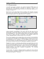
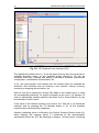
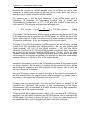
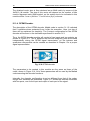
III.1. VPI Transmission Maker as a simulation tool ................................................................. 43
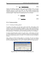
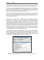
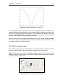
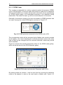
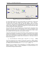
III.1.1. Graphical User Interface .......................................................................................... 43
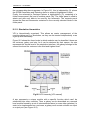
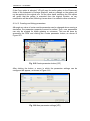
III.1.2. Simulation hierarchies .............................................................................................. 45
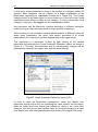
III.1.3. Simulation parameters ............................................................................................. 46
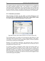
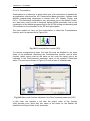
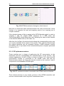
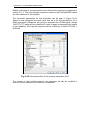
III.1.4. Custom modules....................................................................................................... 48
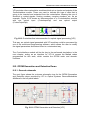
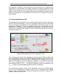
III.2. OFDM Generation and Detection Demo ......................................................................... 52
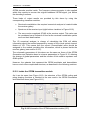
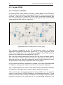
III.2.1. General schematic .................................................................................................... 52
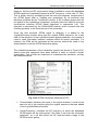
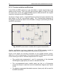
III.2.2. Coder and decoder parameters ............................................................................... 55
III.2.3. Simulation results ..................................................................................................... 56
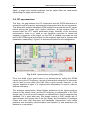
III.3. OFDM for Long-Haul Transmission Demo ....................................................................... 60
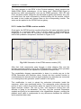
III.3.1. General schematic .................................................................................................... 60
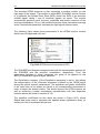
III.3.2. Inside the OFDM transmitter module ...................................................................... 61
III.3.3. Inside the OFDM receiver module ........................................................................... 63
III.3.4. Optical channel path ................................................................................................ 65
III.3.5. Simulation results ..................................................................................................... 67
CHAPTER IV - CUSTOMIZED SIMULATIONS ................................................................................. 70
IV.1. Custom modules and Matlab code implementation ...................................................... 70
IV.1.1. Parameter settings ................................................................................................... 70
IV.1.2. Code structure ......................................................................................................... 72
IV.1.3. OFDM Coder............................................................................................................. 76
IV.1.4. OFDM Decoder......................................................................................................... 78
IV.1.5. RF up/downconverters ............................................................................................ 80
IV.1.6. Sequence comparer ................................................................................................. 82
IV.2. Electrical OFDM Generation and Detection.................................................................... 83
IV.2.1. Universe schematic .................................................................................................. 83
IV.2.2. Raw transmission ..................................................................................................... 85
IV.2.3. Roll-off factor ........................................................................................................... 86
IV.2.4. Zero Padding ............................................................................................................ 87
IV.2.5. Cyclic Prefix .............................................................................................................. 88
IV.2.6. Received Constellation............................................................................................. 89
IV.3. Optical OFDM .................................................................................................................. 90
IV.3.1. Universe schematic .................................................................................................. 90
IV.3.2. Custom modules modifications ............................................................................... 92
IV.3.3. Error Vector Magnitude and Bit Error Rate measuring ........................................... 93
IV.3.4. Reference frequency choice and cyclic prefix extraction ........................................ 95
IV.3.5. Simulation results I: OFDM signal spectra ............................................................... 99
IV.3.6. Simulation results II: Decoded signal ..................................................................... 104
CHAPTER V – CONCLUSIONS AND FUTURE LINES ..................................................................... 109
V.1. Conclusions .................................................................................................................... 109
V.2. Future lines .................................................................................................................... 111
REFERENCES .............................................................................................................................. 112
Books ..................................................................................................................................... 112
Papers and tutorials .............................................................................................................. 112
Websites ................................................................................................................................ 113
ACRONYMS ................................................................................................................................ 114
INTRODUCTION
1
INTRODUCTION
Orthogonal frequency division multiplexing (OFDM) is a widely used modulation
and multiplexing technology, which is now the basis of many
telecommunications standards including wireless local area networks (LANs),
digital terrestrial television (DTT) and digital radio broadcasting in much of the
world. OFDM is also the basis of most DSL standards, though in this context it
is usually called discrete multitone (DMT) because of some minor peculiarities.
Despite the important advantages that OFDM provides and its widespread use
in wireless communications, it is only during the last years that it has been
considered for optical communications [P1]. The lack of interest in optical
OFDM in the past is partly because of the fact that the silicon signal processing
power had not reached the point at which sophisticated OFDM signal
processing could be performed in a CMOS integrated circuit, and partly
because the demand for increased data rates across long fibre distances is
quite recent.
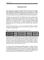
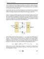
Another important obstacle has been the fundamental differences between
conventional OFDM systems and conventional optical systems. Table 1
summarizes these differences:
Table 1 Typical OFDM system vs. typical Optical system [P1]
Typical OFDM
system
Typical Optical
system
Bipolar
Unipolar
Info carried on
electrical field
Info carried on
optical intensity
LO at receiver
No LO (laser)
at receiver
Coherent
reception
Direct
detection
In typical (non optical) OFDM system, the information is carried on the electrical
field and the signal can have both positive and negative values (bipolar). At the
receiver there is a local oscillator (LO) and coherent detection is used. In
contrast in a typical optical transmission system, the information is carried on
the intensity of the optical signal and therefore it can only be positive (unipolar).
Generally, no laser is used at the receiver acting as a local oscillator and direct
detection rather than coherent detection is used.
An initiative towards the application of OFDM modulation in optical networks is
the Accordance (A Novel OFDMA-PON Paradigm for Ultra-High Capacity
Converged Wireline-Wireless Access Networks), a European research project
in which UPC takes part along with other universities and companies from
around the continent. Within this collaboration, a new communications system is
being developed based on OFDM access technology and protocols.
2
INTRODUCTION
UPC is in charge of performing simulations and feasibility studies for this lowcost, high-capacity hybrid communications system where optical fibre is used as
the transmission channel.
The results described in this Master Thesis will add to the UPC collaboration
within the Accordance project.
The goal in this Master Thesis is to study the basis of OFDM systems applied to
fibre optic networks, both from an analytical point of view and from a simulation
software environment, using the Virtual Photonics Inc. (VPI) software.
The starting point will be the main theoretical concepts that distinguish OFDM
from other modulations, making special emphasis in the peculiarities of its
implementation in optical fibre systems. Then, the main optical OFDM
characteristics are studied and simulated through built-in demonstrations
available at VPI software.
These demos provide a convenient way to study some basic features of OFDM
optical transmission systems, but their use is limited to specific scenarios.
In order to obtain a flexible platform for tests and exploration of optical OFDM
systems a new setup will be built by exploiting the VPI Cosimulation
functionality, which allows the use of other simulation software to operate as
specific modules within VPI.
Thus, in this Master Thesis two VPI modules have been created based on
Matlab programs to perform the OFDM modulator and demodulator inside the
VPI optical OFDM transmission system simulation setup.
While VPI’s built-in demonstrations are quite rigid in terms of configuring
different simulation setups, the use of the Matlab code in the customized
simulations allows the user to perform different configurations for the
transmission scenario which are impossible to obtain from the demos.
The document is organized as follows: In Chapter I, the basic concepts of
OFDM are described, so it can be understood how an OFDM system works and
which is the role of each of its parts. After that, the most typical optical
configurations in which OFDM can be implemented are listed in Chapter II,
giving emphasis to those related with the simulations performed in the last part.
In Chapter III, the basic parameters of VPI software are introduced, and the
required steps to create a new simulation are described. Moreover, two optical
OFDM demonstration scenarios provided by VPI are analyzed in detail, so it
can be seen how the concepts explained in the previous chapters are applied to
a simulation environment.
INTRODUCTION
3
The VPI built-in demos studied in Chapter III will serve as the base for the
customized simulations in Chapter IV, where an insight is given into the main
modules created in VPI for the customized demos. The resulting scenarios will
perform the same functions as the built-in demos in VPI, though this time the
user will be able to change any parameter of the simulation in order to see its
effect on the transmission results. Also, some improvements have been added
to the original functions in the demos, allowing a better understanding of each of
the simulation stages and results.
Conclusions and future lines are developed in Chapter V. This work will set the
basis for upcoming optical OFDM simulations studies, hoping to serve as a
source of inspiration to other contributions to the subject. For this purpose,
propositions to improve the current work as well as the study of other available
optical OFDM techniques to explore are given as a future possibility.
Furthermore, 4 Annexes are attached, which are referred along the work. They
contain complementary theoretical information, as well as secondary
configurations for possible simulated scenarios. The last of them shows the
Matlab code used in the simulations.
4
FIBER-BASED OFDM TRANSMISSION SYSTEMS
CHAPTER I - OFDM BASICS
I.1. General idea
Frequency Division Multiplexing (FDM) is a technique where the main signal to
be transmitted is divided into a set of independent signals, which are called
subcarriers in the frequency domain. Thus, the original data stream is divided
into many parallel streams (or channels), one for each subcarrier. Each
subcarrier is then modulated with a conventional modulation scheme, and then
they are combined together to create the FDM signal.
In an FDM transmission, the receiver needs to be able to independently recover
each of the subcarriers and therefore these signals need to fulfil certain
conditions. For instance, they can have nonoverlapping spectra so that a bank
of filters tuned to each of the different subcarriers can recover each of them
independently. However, practical filters require guard bands between the
subcarrier bands and therefore the resulting spectral efficiency is low.
If the subcarrier signals fulfil the orthogonality condition (which will be
introduced by expression I.2) their spectrum can overlap, improving the spectral
efficiency. This technique is known as orthogonal FDM or OFDM.
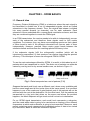
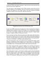
To see the main advantages offered by OFDM, it is useful to think about a set of
packets which are transported in a truck. The whole set of packets can either be
carried by one big truck or by several smaller ones, as shown in Figure I.1:
Fig. I.1 Data transported as a set of packets [P18]
Suppose that each small truck uses a different road, where every available path
has the same length and all the trucks drive at the same speed. If an accident
happens in one of the roads and it gets blocked, part of the packets will not be
received with the rest at the destination. On the other hand, if all the packets are
transported by a big truck that drives on the same road where the accident
happens, the whole shipment will get stuck and will not arrive to destination.
For an OFDM signal transmission, each small truck represents a subcarrier,
and the roads where data is going to be carried are an analogy of the different
frequencies at which each subcarrier is going to be transmitted. Moreover, each
packet containing goods represents the modulated portion of data to be carried
by a subcarrier, which is called an information symbol.
CHAPTER I – OFDM BASICS
5
Then, continuing with the analogy, it should be more difficult to drive a big truck
than a smaller one, meaning that transmission impairments will have a bigger
impact on the single carrier signal since, in the transmission case, it will have to
be transmitted at a higher data rate.
On the other hand, for a transport company it is more expensive to contract N
small trucks than a big one. In the transmission case, this is equivalent to the
difference between using N emitter-receiver sets and using a single one.
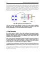
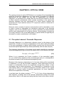
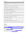
Figure I.2 shows the OFDM modulation idea schematically. A bit sequence with
rate R is parallelized into N different channels, each with a different frequency.
The total bitrate is distributed in equal parts over each channel at a rate R/N.
The data in each channel will be mapped to represent an information symbol
and then multiplied by its corresponding frequency. The summation of these
parallel information symbols will form one OFDM symbol.
Fig. I.2 Frequency division multiplex: Analogue transmitter
Each OFDM symbol has thus a duration
. Hence, the OFDM signal in
the time domain s(t) can be expressed as a summation of each information
symbol
being carried in the kth subcarrier within the ith OFDM symbol.
Depending on the modulation used for the subcarriers, this superposition of
subcarriers forming s(t) can result in complex values, though this case will not
be taken into account yet. Then, with the OFDM symbol having a period :
(I.1)
Where P(t) is an ideal square pulse of length , the number of subcarriers is
represented by N and
is the subcarrier frequency. This frequency has to fulfil
the orthogonality condition:
(I.2)
6
FIBER-BASED OFDM TRANSMISSION SYSTEMS
This means that each subcarrier must be separated from its neighbours by
exactly 1/ , so each subcarrier within an OFDM symbol has exactly an integer
number of cycles in the interval , and the number of cycles differs by exactly
one, as depicted in Figure I.3. This way, orthogonality between subcarriers is
achieved. This property can be explained for any couple of subcarriers by the
following expression:
,
(I.3)
If m and n are different natural numbers, the area under this product over one
period is zero. The frequencies of these waves are called harmonics and for
them the orthogonality condition is always fulfilled.
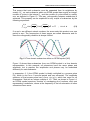
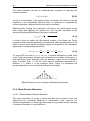
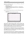
Fig. I.3 Time domain subcarriers within an OFDM symbol [W2]
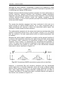
Figure I.3 shows three subcarriers from one OFDM symbol in a time domain
representation. In this example, all subcarriers have the same phase and
amplitude, but in practice the amplitudes and phases may be modulated
differently for each subcarrier.
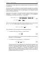
In expression (1.1) the OFDM symbol is ideally multiplied by a square pulse
P(t), which is one for a -second period and zero otherwise. The amplitude
spectrum of that square pulse has a form
, which has zeros for all
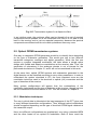
frequencies f that are an integer multiple of 1/ . Then, as shown in Figure I.4,
an OFDM symbol spectrum consists of overlapping sinc functions, each one
representing a subcarrier, where at the frequency of the kth subcarrier all other
subcarriers have zeros.
CHAPTER I – OFDM BASICS
7
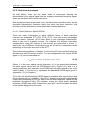
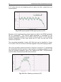
Fig. I.4 Spectrum of an OFDM symbol with overlapping subcarriers [P2]
Note that each subcarrier is centred at
and separated by 1/Ts from its
neighbours. When this happens, the orthogonality condition is being fulfilled so
a great spectral efficiency for the transmission is achieved. This way, the
subcarriers can be recovered at the receiver without intercarrier interference
(ICI) despite strong signal spectral overlapping, by means of the orthogonality
condition (1.3) using a bank of oscillators and low-pass filtering for each
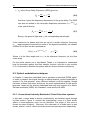
subcarrier, as shown in Figure I.5
Fig. I.5 Frequency division multiplex: Analogue receiver
Note that many analogue components are needed in case of using a large
number of subcarriers. This factor gives rise to a tradeoff between the desire to
8
FIBER-BASED OFDM TRANSMISSION SYSTEMS
use as many subcarriers as possible to make the OFDM signal stronger against
transmission impairments, and the system complexity associated to the use of
analogue components, especially when many of them are needed.
In single carrier systems, the symbol period is given by the reciprocal baud rate
1/R. Since in multicarrier systems such as OFDM the symbol period is N times
longer, the effect of channel dispersion is typically lower and the inter-symbol
interference (ISI) decreases. Moreover, as it will be seen in the next section, ISI
can be almost eliminated by introducing a guard time in every OFDM symbol
such that most of the dispersion caused by a multipath channel remains within
the guard interval.
It will also be explained later that in the guard time, the OFDM symbol is
cyclically extended to avoid generating ICI. In single-carrier systems ISI occurs
and can only be compensated by using complex equalizers at the receiver. In a
multicarrier system, no equalization to overcome ISI is required and only the
amplitude and phase of each subcarrier need to be corrected according to the
channel frequency response. This is simply done by one complex-valued
multiplication per subcarrier, which is in fact a single-tap equalization.
I.2. Digital generation of subcarriers
I.2.1. Fast Fourier Transform
Following the last section’s analogy, the more trucks are used to transport the
load, the fewer packets are going to be carried by each one, the easier it is for
each truck to complete the journey, and the less load is going to be lost in case
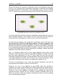
of an accident. Then, it can be said that in an OFDM transmission a large
number of subcarriers is desirable so that the minimum possible quantity of data
is lost in case of any non-ideality occurring in the transmission channel. This
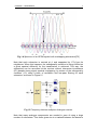
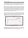
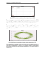
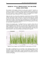
effect is shown in Figure I.6:
Fig. I.6 OFDM subcarriers affected by a fading channel [P18]
However, creating an OFDM signal with a large number of subcarriers following
the analogue method presented before leads to an extremely complex
CHAPTER I – OFDM BASICS
9
architecture involving many oscillators and filters at both the transmit and
receive ends. In present-day OFDM transmissions, though, this complexity is
reduced by transferring it from the analogue to the digital domain.
To see this, take Equation (I.4), where just one OFDM symbol of the signal s(t)
in (I.1) is sampled at an interval of
. Then, the
sample of s(t) becomes:
(I.4)
Where is the Fourier transform, and n [1,N]. Thus, it can be said that the
discrete value of the transmitted OFDM signal s(t) is merely a simple N-point
inverse discrete Fourier transform (IDFT) of the information symbol . The
same case can be applied at the receiver, where the received information
symbol will be a simple N-point discrete Fourier transform (DFT) of the received
sampled signal.
This superposition of independent modulated subcarriers is typically performed
by the inverse fast Fourier transform (IFFT) where the input channels are
spaced equivalently according to Expression I.2. In fact, IFFT/FFT blocks in an
OFDM system are mathematically equivalent versions of an IDFT and a DFT of
the transmitted and received OFDM signal, with the advantage of providing
lower computational implementation.
Because of the orthogonality property, as long as the channel is linear, the
OFDM receiver will calculate the spectrum values at those points corresponding
to the maximum of individual subcarriers. Then, the received subcarriers can be
demodulated through an FFT operation without interference and without the
need for analogue filtering to separate them, which makes OFDM not only
efficient but also easy to implement in practical transmission systems.
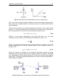
Hence, it can be said that the modulated OFDM signal can be obtained by
performing the IFFT operation to the symbols to transmit and then using a DAC
to convert the digital signal into an analogue signal at a sampling rate Ts.
Ideally, this D/A conversion should convolve each temporal sample by a sinc
function. This ideal shaping is translated into a perfectly rectangular filter that
removes the alias in the frequency domain, as shown in Figure I.7:
Fig. I.7 Ideal filter at the DAC [VPI]
10
FIBER-BASED OFDM TRANSMISSION SYSTEMS
Where
is the Nyquist frequency, which will be the highest frequency
component of the OFDM signal. This ideal filter will remove the alias generated
due to the sampling process, leaving the fundamental signal untouched.
The contribution of the different sinc pulses at each of the samples of the OFDM
symbol results in a perfect square pulse of the OFDM symbol, and each of the
subcarriers would be represented by a perfect sinc function in the frequency
domain.
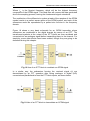
Figure I.8 shows a very basic schematic for an OFDM transmitter where
subcarriers are modulated in the digital domain by means of an IFFT. The
transformed symbols at the output of the IFFT block are then serialized and
converted into an analogue signal before transmitting them to the channel. For
simplicity, some other blocks have been omitted, though they are going to be
described during this chapter.
Fig. I.8 Use of an IFFT block to modulate an OFDM signal
In a similar way, the subcarriers forming the received signal r(t) are
demodulated by an FFT operation after being analogue to digital (A/D)
converted and parallelized to form the FFT block inputs, as shown below.
Fig. I.9 Use of an FFT block to demodulate an OFDM signal
CHAPTER I – OFDM BASICS
11
In order to understand the concepts that are going to be explained in the next
sections, it is useful to know which frequencies of an OFDM signal are
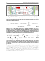
represented in each branch of an IFFT operation. Figure I.10 shows a
schematic of the IFFT block, where
are the input sequence symbols
from subcarrier 1 to the total number of subcarriers N, and
is the
corresponding output sequence. Moreover, the frequency domain OFDM
symbol generated at the IFFT output is depicted. The inverse procedure can be
applied to the FFT block at the receiver end.
Fig. I.10 IFFT block and the frequency domain OFDM symbol at its output [P4]
The first output channel ( ) is located at DC, so it is not used for modulation
because carrier leakage of the modulator disturbs the quality of this channel
and it would put stringent requirements on the low-pass characteristics of all
electronic (and also optic) components.
Furthermore, in a complex valued IFFT the first half of the rows corresponds to
the positive frequencies while the last half corresponds to negative frequencies.
Thus, the so called “Nyquist channel” is located at yNc/2+1, which corresponds to
the highest frequency that the subsequent digital-to-analogue converter can
modulate: the Nyquist frequency (fN), or half the sampling frequency
according to the sampling theorem.
In a practical system, if the superposition of subcarriers results in complex
valued time domain signals, two D/A converters may be applied in parallel for
conversion of the real and imaginary IFFT output, though other techniques like
the imposition of Hermitian symmetry among samples can be applied in order to
have a perfect real IFFT output, as explained in Annex A.
I.2.2. D/A and A/D conversion
As it can be seen from figures I.8 and I.9, a digital-to-analogue converter (DAC)
is needed to convert the discrete value of
(
sample) to the continuous
analogue value of s(t), and an analogue-to-digital converter (ADC) is needed to
convert the continuous received signal r(t) to discrete sample .
12
FIBER-BASED OFDM TRANSMISSION SYSTEMS
In order to build a real system, the fact of being able to use commercial off-theshelf converters at both ends of the transmission scheme becomes one of the
main issues. This is why many techniques are available to take advantage from
the digital signal processing stages and simplify the analogue processing,
lowering the requirements for both the DAC and the ADC.
I.2.2.1 Pulse shaping
Inside the DAC, symbols are applied to a transmit filter, which produces a
continuous-time signal for transmission over the continuous-time channel. A
simple transmit filter has a rectangular impulse response, shown in figure I.11,
where a symbol sequence using 2 bits per symbol and its corresponding
continuous-time signal are also represented.
Fig. I.11 Rectangular impulse response [B6]
The impulse response g(t) of the transmit filter is called the pulse shape. The
output of this filter is the convolution of the pulse shape with the symbol
sequence, so the resulting signal can be interpreted as a sequence of possibly
overlapped pulses with the amplitude of each determined by a symbol.
An ideal low-pass filter as the one represented in Figure I.7 has a sinc function
impulse response with equidistant zero-crossings at the sampling instants and
hence no ISI. However, this ideal filter is not realizable.
A practical extension is a raised cosine characteristic fitted to the ideal low-pass
filter, which is a commonly used pulse shape in OFDM. Its transfer function is
given by expression I.5:
(I.5)
Here,
is the symbol period and α is the roll-off factor, defined as the ratio of
excess bandwidth above . When α = 1 the bandwidth is doubled over the
bandwidth when α = 0. The impulse response of the raised cosine filter used in
CHAPTER I – OFDM BASICS
13
VPI for α = 0 and α = 0.5 is shown in figure I.12 Note that the length is reduced
at the expense of increased bandwidth.
Fig. I.12 Impulse response for the raised cosine for α = 0 and α = 0.5 [VPI]
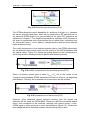
I.2.2.2 Oversampling by means of zero padding
Before giving the OFDM signal its corresponding shape, the values at the
output of the IFFT representing the analogue signal to transmit have to be
sampled by the DAC. By sampling them at a rate of 1/ , the aliases produced
by the sampling process would be right next to the main OFDM signal, making it
impossible for any practical filter to separate them.
However, padding the correct positions of the IFFT input sequence with zeros
can help to shift the aliases away from the OFDM signal, as shown in Figure
I.13. This technique will be referred during this work as oversampling or
frequency zero padding.
Fig. I.13 Oversampling used to shift aliases away [P4]
14
FIBER-BASED OFDM TRANSMISSION SYSTEMS
Note that the zero-padded frequencies are those around the Nyquist channel.
This ensures the zero data values are mapped onto the highest positive
frequencies and lowest negative frequencies (those around
), while the
nonzero data values are mapped onto the subcarriers around 0 Hz, preserving
the main OFDM signal.
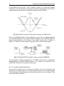
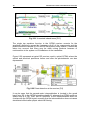
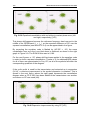
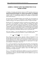
The reason why the aliases are shifted away from the OFDM signal can be
understood by looking at Figure I.14. In the upper case no oversampling is
applied, while the lower case represents a typical 2xoversampling transmission,
where half of the IFFT inputs (those in the centre around the Nyquist frequency)
have been used for zero padding in the same way as in Figure I.13. In this
case, the number of IFFT inputs has to be doubled in order to allocate the same
number of OFDM subcarriers as before.
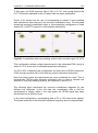
The input sequences of the IFFT are represented in the left side. After
performing the IFFT operation, the sampled signal is obtained (centre figures).
Note that twice the number of samples is used to represent that signal in the
case of using oversampling. The D/A conversion carried out in the DAC is
understood as temporal extrapolation / frequency-alias filtering of this sampled
signal.
Fig. I.14 Aliases moving away due to zero padding
If the spectrums of these analogue signals are represented by applying the
Discrete-time Fourier transform (DTFT), it can be seen how the oversampled
signal spectrum becomes narrower.
This narrowing effect is produced because the high frequencies are zero
padded, though the same quantity of information is still being added over the
same bandwidth, so the spacing between subcarriers is decreased.
This will cause a frequency separation between the maximum frequency of the
OFDM signal and the minimum frequency of the subsequent alias. Thus, the
requirements of the filter needed to recover the original signal will not be too
high, enabling the choice of a non-expensive DAC for the system.
This technique will be applied in the simulations performed in chapter IV by
using the same number of IFFT inputs for information symbols and for zeros.
CHAPTER I – OFDM BASICS
15
For instance, a 128 IFFT/FFT size will be used to apply the oversampling
technique when the information is coded into 64 OFDM subcarriers.
I.2.3. Cyclic Prefix
As mentioned before, by dividing the data stream into N subcarriers, the symbol
period is made N times longer, which also reduces the delay spread or
chromatic dispersion relative to the symbol time. To avoid interferences
between OFDM symbols (meaning null ISI) and also eliminate ICI, a guard time
is introduced for each OFDM symbol after the IFFT, which is cyclically extended
within this guard time, as shown in Figure I.15. This cyclical extension is called
the cyclic prefix (CP).
Fig. I.15 Cyclic prefix in an OFDM symbol (time domain sequence) [P4]
Due to the insertion of this prefix, the symbol duration is extended without
transmission of additional data, leading to a reduction of the net bitrate by a
factor of
, where
is the extension of the symbol period due to the
cyclic prefix . However, the simple equalization resulting from the elimination of
both ISI and ICI from the received signal is a major advantage which deserves
giving up a bit of transmission efficiency.
As long as the cyclic prefix duration is equal or longer than the maximum delay
caused by the channel impairments, the effect of one symbol over its
neighbours will be limited to its cyclic prefix corruption, without damaging the
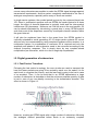
information part. The effect of a cyclic prefix length shorter than the drift caused
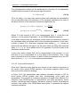
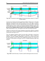
by chromatic dispersion in optical OFDM is shown in Figure I.16, where an
OFDM signal is represented with different colours for each subcarrier:
It is true that null ISI could be achieved with the introduction of any temporal
guard interval, but only the cyclic prefix can guarantee null ICI. This fact is
mathematically demonstrated in [P1].
It is important to mention that the introduction of cyclic prefix entails the loss of
orthogonality in the transmitted symbols, though this will not be a problem, as
this cyclic extension will be eliminated in the receiver recovering the original
orthogonality [B7].
16
FIBER-BASED OFDM TRANSMISSION SYSTEMS
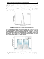
Fig. I.16 ISI because an insufficiently large CP [P4]
Another interesting effect can be observed in the OFDM signal spectrum: when
the temporal duration of the OFDM symbol is increased due to the CP insertion,
the corresponding sincs are narrower in frequency than before, so their
maximums don’t match up exactly with their neighbours’ nulls and the resulting
spectrum is not plain any more, but it suffers from rippling. This effect is dealt
with in Annex B, where the consequences of adding a CP on the signal
spectrum are discussed.
In the simulations performed with VPI, the cyclic prefix parameter will be
determined by a percentage of the total number of symbols at the output of the
IFFT block. The typical values for a cyclic prefix in an OFDM system range from
10 to 20%.
In view of all the above, the final schematic for the OFDM signal generation
could be represented by the one in Figure I.17, where oversampling by means
of frequency zero padding and a temporal cyclic prefix are added in the
following order:
Fig. I.17 OFDM signal generation schematic
CHAPTER I – OFDM BASICS
17
At the receiver end, zero padding and cyclic prefix are extracted in the opposite
order in which they were inserted at the transmitter, as shown in Figure I.18:
Fig. I.18 OFDM signal reception schematic
Now that the electrical OFDM signal is ready to be transmitted, it needs to be
re-modulated over an optical carrier to be transmitted through an optical
channel. For this purpose, different methods of optical modulation and detection
are presented in Chapter II, but before that, Section I.3 will serve as an
introduction to the used method in the optical OFDM simulations.
I.2.4. Mapping and demapping
It has been said before that the bit stream coming from the signal source needs
to be converted into many parallel data pipes, each mapped onto corresponding
information symbols for the subcarriers within one OFDM symbol.
The incoming bits to send have to be packed and mapped to a symbol generally
using a complex modulation format such as for example M-QAM or QPSK.
For the 4-QAM modulation used in this work’s simulations, the incoming serial
data uses two bits to create each of the 4 possible complex-valued QAM
symbols (or information symbols), as it can be seen from Figure I.19:
Fig. I.19 4-QAM mapping [P4]
18
FIBER-BASED OFDM TRANSMISSION SYSTEMS
The inverse procedure will take place at the receiver side: each complex-valued
received symbol will be demapped and the obtained symbol sequence will be
serialized to (ideally) obtain the original bit stream from the transmitter.
However, because data is not going to be transmitted over an ideal channel, a
decision of which constellation point is received has to taken before demapping.
This process is called slicing, and it is depicted in Figure I.20:
Fig. I.20 4-QAM slicing and demapping [P4]
The most commonly used method for slicing is a hard decision threshold,
though many other methods have been introduced to perform it with soft
decision thresholds at a cost of an increased system complexity.
I.3. Gap generation
As it can be seen in Chapter II, when the conventional opto-electrical directdetection technique is used in the receiver, due to the square-law characteristic
unwanted mixing products among the subcarriers may interfere with other
subcarriers in the electrical domain.
Also, when using the conventional intensity modulation technique, replicas of
the signal appear on the optical spectrum. In order for these replicas not to
overlap with the OFDM signal, guard bands with respect to the optical carrier
are also required. This is described in more detail in Chapter II.
To prevent these interferences a frequency gap may be allocated between the
optical carrier and the OFDM spectrum, which width at least equals that of the
signal’s bandwidth.
In this section two strategies to create a spectral gap between the carrier and
the OFDM spectrum are described, namely the RF upconversion and the lowfrequency zero padding.
CHAPTER I – OFDM BASICS
19
I.3.1. RF upconversion
In the RF upconversion technique, the complex baseband OFDM signal s(t)
generated with QAM subcarrier modulation as depicted in Figure I.17 is
upconverted into a passband signal centred at an intermediate frequency (IF),
as shown in Figure I.21.
Note that the cyclic prefix stage has been omitted in this schematic, though it
will be used in the simulation. Also, note that two DACs are used to process the
real and imaginary parts of the signal after the IFFT operation.
Fig. I.21 RF upconversion [P6]
In this schematic, oversampling is first used to shift the alias away from the
OFDM signal, and then the frequency upconversion is done to create a gap in
the electrical spectrum. The real and imaginary parts of the signal are separated
after the IFFT stage, and after its conversion to the analogue domain the
complex baseband signal is obtained (lower inset of the figure).
The real and imaginary parts corresponding to the in-phase (I) and quadrature
(Q) components of the signal are then passed through an electrical IQ mixer for
its upconversion to an IF, namely . For this purpose, there must be a 90º
phase shift between the locally generated carrier at IF frequency that multiplies
the in-phase component and the one multiplying the quadrature component.
Despite the increase in complexity of the analogue part entailed by the use of
an RF upconversion stage, the IFFT/FFT size and the DAC bandwidths could
be fully used to process useful data in order to lower the DAC requirements.
Alternatives exist to this configuration, sometimes involving a tradeoff between
reduced efficiency and lower complexity arrangements. The following
subsection is good example.
At the receiver, the signal is downconverted by another IQ mixer with the
opposite function, returning the OFDM signal to baseband before extracting the
CP and performing the FFT operation.
20
FIBER-BASED OFDM TRANSMISSION SYSTEMS
I.3.2. Zero padding at the edges of the IFFT input sequence
This is another way to create a gap between the OFDM signal and the DC
component which allows avoiding the problems carried by the use of analogue
mixers and oscillators.
As shown in Figure I.22, zeros are added at the beginning and at the end of the
IFFT input sequence. The more zeros are added, the larger will be the created
gap, though the bitrate efficiency will decrease.
Fig. I.22 Gap created by zero padding [P4]
In the same way as in the RF upconversion case, this gap will serve as a guard
band between the OFDM subcarriers and the optical carrier when optical
modulation is applied. This will be used to avoid unwanted mixing products both
in emission when using IM modulation and at the receiver when using DD.
This form of zero padding can be used at the same time as the oversampling
method when creating the input sequence for the IFFT, obtaining a signal with
remote aliases and a guard band close to DC, though it can result in quite a
reduction of the spectral efficiency. Thus, this trade-off between low complexity
of the receiver and spectral efficiency of the transmission will be decisive in the
resulting configurations.
I.4. General system schematic
By putting together all the concepts explained until now, the final appearance of
an OFDM system could be the one depicted in Figure I.23.
In order to correct the channel’s response, a single-tap equalizer should be
used at the receiver end to calculate any possible phase shift.
The optical modulation and demodulation stages, as well as the channel
impairments affecting an OFDM transmission over optical fibre are explained in
detail in the next chapter.
CHAPTER I – OFDM BASICS
21
Fig. I.23 OFDM system schematic
Before the RF upconversion, s(t) is approximately bandlimited, consisting of
sinusoids of the baseband subcarrier frequencies. For the simulations carried
out in this work, the signal
after the RF mixer will form the electrical input
to an optical modulator after being upconverted to the carrier frequency. Thus,
the upconverted electrical OFDM signal at the output of the front end block is:
(I.7)
Where s(t) is the complex baseband OFDM signal as in (I.1). For wireless
systems, this signal could be modulated by a complex IQ modulator and then
transmitted. Otherwise, it would be necessary to transmit real quantities, which
can be accomplished by first appending the complex conjugate to the original
input block. See Annex A for a detailed description of the process.
22
FIBER-BASED OFDM TRANSMISSION SYSTEMS
CHAPTER II - OPTICAL OFDM
The growing interest for optical OFDM due to an increase of the demanded data
rates has fostered the appearance of a large variety of solutions for different
applications, so this chapter will deal with its classification into different
categories. The preference for simple and low-cost solutions based on the use
of direct detection photodiodes which operate according to the square-law
detection technique and the requirement of a linear system between the
transmitter IFFT input and the receiver FFT output are common in almost all of
these solutions.
Moreover, basic concepts of optical communications will be described in order
to make it easier to understand the simulations performed in the following
chapters, such as the available types of optical modulation and demodulation
and the main characteristics of an optical channel. Some of these concepts are
not usually referred in the current bibliography of optical OFDM, though they are
the basis for creative contributions to the subject.
II.1. The optical channel: Chromatic Dispersion
Chromatic dispersion is a deterministic distortion given by the design of the
optical fibre. It leads to a frequency dependence of the rate at which the phase
of the wave propagates in space (optical phase velocity) and its effect on the
transmitted optical signal basically scales quadratically with the data rate [P2].
This frequency dependence of the phase can be easily identified by describing
a pulse propagating through a monomode optical fibre in the frequency domain:
(II.1)
Where
represents the Fourier transform of the transmitted signal,
is the Fourier transform of the received signal and
corresponds to
the phase constant of the fundamental propagating mode.
Because of the frequency dependence of , the main limiting effect considered
in expression (II.1) will be chromatic dispersion. Other phenomena such as
losses or nonlinearities will be not considered, though their effects in fibre
propagation can be added afterwards. The consideration of dispersion as the
main limiting effect in an optical transmission has been shown to be a good
approach in a broad variety of practical applications, but more importantly
allows the simplification of its study.
In an ideal case, the phase constant
in (II.1) has a linear dependency
with frequency, meaning that all the spectral components undergo the same
phase delay, which is the same as saying that they travel at the same velocity.
CHAPTER II – OPTICAL OFDM
23
At reception the same signal will be obtained without any distortion but with a
constant delay.
On the other hand, in a dispersive channel the phase constant has a nonlinear
dependency with frequency and as a consequence of the different arrival times
of the frequency components, the recovered signal at the reception end will
differ from the transmitted one.
Assuming a slow variation of the phase constant inside the signal’s frequency
bandwidth, it is possible to consider a Taylor expansion of the propagation
constant about a central pulse frequency
as follows:
    o   2     o   3 
      0      o 




2
6
 2
 3
 2
 3
  o   1 
2 
3  
2
6
2
3
(II.2)
Where the third and higher order terms can be neglected if it is considered that
, which enables the possibility to rewrite (II.2) as:
(II.3)
The coefficients in (II.3) are related to the following parameters:

relates to the Phase Velocity
, which verifies:
(II.4)
And it can be defined as the velocity at which the phase of a pure tone at
frequency
would propagate.

is related to the Group Velocity
, of the pulse by:
(II.5)
The group velocity can be defined as the rate with which changes in the
envelope of the wave (amplitude) propagate. The Group Delay , given
in (II.5) in seconds/fibre length, gives the delay experienced by an
envelope centred at frequency
, provided its bandwidth is not too
large, as the Taylor expansion would no longer be valid. It can also be
thought that this delay is a kind of average delay of all the frequencies in
a small bandwidth around the carrier.
24
FIBER-BASED OFDM TRANSMISSION SYSTEMS

is the Group Delay Dispersion (GDD) given by:
(II.6)
And thus it gives the frequency dependency of the group delay. The GDD
can also be related to the chromatic dispersion parameter (
)
of an optical fibre by:
(II.7)
Being c the speed of light and
the corresponding wavelength.
If the references for phase and time are set at a certain reference frequency
(
) approximately located at the centre of the signal’s bandwidth, the transfer
function of the fibre can be expressed as:
:
,
Where L is the fibre length and
under study.
(II.8)
is the reference frequency for the fibre
For the works carried out in this Master Thesis, it is important to understand
how the simulator applies this fibre transfer function, and this is why section
IV.3.4 is devoted to describe its relation with the chosen reference frequency.
II.2. Optical modulation techniques
In Chapter I, it has been described how to generate an electrical OFDM signal.
In order to transmit this signal through an optical channel, optical modulation is
required. For that purpose, many different methods could be applied, though
just three of them have been chosen as the most representative for this work’s
purposes: those are the directly modulated laser and two versions of a MachZehnder modulator (MZM): the “standard” mode and the IQ MZM.
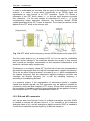
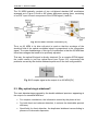
II.2.1. Conventional Intensity Modulated / Direct Detection systems
In this case, a laser diode is directly modulated by an electrical signal through
its bias current. Figure II.1 shows the characteristic curve of a laser diode,
where a linear-behaviour zone can be identified. The slope of this zone is
known as slope efficiency. Moreover, the schematic of a diode laser is also
shown, where IL and P0 refer to the bias current and optical power, respectively.
CHAPTER II – OPTICAL OFDM
25
Fig. II.1 Schematic and characteristic curve of a laser diode
This is the most straight-forward method to send information through optical
fibre, based on causing variations of the bias current of a diode laser above a
given threshold.
These current variations ( ) lead to proportional variations of the output optical
power
, which are detected by a PIN diode at the receiver end, carrying out
the reverse process to recover the sent information signal s(t), as:
(II.9)
Where
is the power associated to the laser bias and m is the used
modulation index, which is also related to the laser bias current as:
(II.10)
Finally, the total received intensity for an ideal channel is a function of the PIN
diode’s responsivity R and the different gains of the amplifier devices in
reception (G):
(II.11)
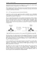
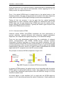
Figure II.2 shows an example of an electrical information signal s(t) being
modulated over an optical carrier. At the emission stage, the signal is converted
from the electrical into the optical domain (E/O), and vice versa at the reception
stage (O/E). This kind of optical transmission is known as Intensity Modulation /
Direct Detection (IM/DD).
Fig. II.2 Schematic of an Intensity Modulation and Direct Detection
26
FIBER-BASED OFDM TRANSMISSION SYSTEMS
The direct detection process is mathematically equivalent to applying the
squared modulus:
(II.12)
As this is a modulation of the optical power or intensity (not directly from the
amplitude of the transmitted electrical field), its spectrum is composed by
various sidebands, replicas from the one being modulated.
Mathematically, starting from expression (II.9) about the optical power at the
laser output and applying the square root, the low-pass equivalent of the
electrical field being transmitted on the fibre is obtained:
(II.13)
In order to give an insight into the spectral content of the signal, the Taylor
expansion of the previous expression is considered, obtaining expression (II.14)
where it can be seen that the modulated signal is composed by the information
signal and its corresponding harmonics:
(II.14)
For a pure RF tone, that is,
, if Intensity Modulation is used, each
of the Taylor series terms will give rise to harmonics at multiples of frequency
with amplitudes which decrease with the harmonic order, as the modulation
order is smaller than 1. This will cause several sidebands separated at a
distance
, where
is the harmonic order. Figure II.3 represents the
resulting spectrum for an intensity modulated optical signal.
Fig. II.3 Spectrum of an intensity modulated optical signal
II.2.2. Mach-Zehnder Modulator
II.2.2.1. Standard Mach-Zhender Modulator
The direct modulation of a laser is cheap and also easy to adapt to low cost
applications for moderated distances or transmission rates. However, for
advanced applications involving high data rates or long distance links, resorting
to external modulation is a good solution.
CHAPTER II – OPTICAL OFDM
27
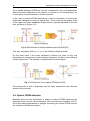
The most typical external modulator is the Mach-Zehnder modulator (MZM),
which modulates the light generated in a laser operating in continuous wave
mode. The MZM has typically an RF input and another input for a DC bias, as it
can be seen from Figure II.4:
Fig. II.4 Mach-Zehnder modulator [VPI]
The material for the MZM has electrooptical properties by which the phase of
the optical wave propagating inside it receives a phase modulation proportional
to the applied electrical field. Therefore, the optical power
at the output of
the MZM depends on the phase difference
between the two arms of the
modulator, which can be changed by varying the bias of the MZM:
,
(II.15)
Where d(t) is the MZM power transfer function and
and
are the
phase changes in each arm caused by the applied modulation signal s(t).
Figure II.5 shows the Intensity Modulation schematic and transfer function for a
MZM, where the bias point is situated in the linear zone of the transfer function
in order to obtain a linear intensity-to-optical power relationship (IM). This point
is known as the quadrature point and is the most used in combination with DD.
Fig. II.5 IM with Mach-Zehnder modulator
By changing the bias of the MZM, the phase of its two arms is shifted. Hence,
the so called Optical Field Modulation mode can be achieved by setting the bias
28
FIBER-BASED OFDM TRANSMISSION SYSTEMS
of the MZM to the null point. This is shown in Figure II.6, where the transfer
functions of the optical intensity and optical field are represented, and the drive
voltage determines the type of modulation performed by the MZM:
Fig. II.6 Transfer functions of the optical intensity and optical field
Either if the MZM is biased in the quadrature or null point, the signal produced
by a standard MZM is a so called “double sideband”, as the OFDM signal is
present symmetrically at both sides of the optical carrier. This is shown in
Figure II.7, where A* is the complex conjugate of the main OFDM signal A.
Fig. II.7 Optical OFDM modulation using a standard MZM [P4]
The duplicated sideband generated by the MZM entails some considerable
disadvantages for optical OFDM systems, so it needs to be removed by an
optical filter. Section II.3 describes this process.
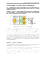
II.2.2.3. IQ Mach-Zehnder Modulator
The previous solution does not make an efficient use of the spectrum and
depends on the performance of the optical filters being used, so another option
of modulating an electrical signal onto an optical carrier can be considered. This
is the optical IQ modulation.
CHAPTER II – OPTICAL OFDM
29
The IQ MZM basically consists of two null-biased standard MZ modulators
arranged as in Figure II.8 with a 90º phase difference among them, consisting
of one RF input for each component of the OFDM signal (I and Q).
Fig. II.8 IQ Mach-Zehnder modulator [P4]
Thus, an IQ MZM in its bias null-point is used so that the envelope of the
electrical field of the optical modulated signal is proportional to the information
signal. The main disadvantage of this type of modulation is that the IQ MZM has
three bias voltages that need to be precisely adjusted.
This way, the optical IQ signal is directly obtained. For a complex OFDM signal,
the output results in just one optical band (see Figure II.9), overcoming the
problems caused by the double sideband spectrums in the last configurations.
Fig. II.9 Complex signal at the output of an IQ MZM [P4]
II.3. Why optical single sideband?
The main disadvantages caused by the double sideband spectrum appearing at
the output of a standard MZM are:

For complex modulations, the information carried by the phase is lost

For both direct and coherent detection, it reduces the obtainable spectral
efficiency

Specifically for direct detection, the duplicated sideband causes fading in
presence of chromatic dispersion.
30
FIBER-BASED OFDM TRANSMISSION SYSTEMS
Thus, double sideband OFDM will only be considered for low cost applications
where chromatic dispersion is not present, or at least is not a limiting factor, as
in free-space communications or access networks.
In the case of optical OFDM applications, it will be necessary to remove the
duplicated sideband by using an optical filter. This is because the phase shifts
of the upper and lower sidebands always result in symbols allocated in the real
axis, as shown in Figure II.10:
Fig. II.10 Detection of double sideband optical OFDM [P6]
This way, any phase shift of
will null the subcarrier power.
On the other hand, if the lower sideband is filtered out, there is only one
photodetection component at each electrical frequency, so there is no nulling at
certain frequencies. This situation is represented in the next figure:
Fig. II.11 Detection of one optical OFDM band [P6]
The phase shift
due to dispersion can be easily equalized in the electrical
domain at the receiver.
II.4. Optical OFDM detection
Basically there are two techniques in which an optical OFDM signal can be
detected at the receiver: direct detection (DD) and coherent detection (CO-D).
All of the existing applications or designs concerning an optical OFDM receiver
are variations of these two options.
CHAPTER II – OPTICAL OFDM
31
Although the direct detection configuration is going to be explained in detail
throughout this chapter, it is important to introduce its principle of operation prior
to describing each optical OFDM system.
Despite coherent detection-based systems represent the best performance in
receiver sensitivity, spectral efficiency and robustness against polarization
dispersion, this work will be mainly focused on direct detection. This is because
coherent detection-based systems require the highest complexity in the
transmitter design, so just its main operation principle will be briefly introduced
at the end of this chapter.
The square-law detection technique has been mentioned in this work as a
typical solution for optical OFDM systems. As no other components than a
single photodiode are required to detect the transmitted optical signal, this
technique is usually known as direct detection.
The mathematical expression for the square-law technique and the study of the
spectral components derived from it can be found in section II.5.2, but before
that, an overview of its main repercussions within an optical transmission can
be realized.
Because the optical signal is obtained in reception as the squared modulus of
its electric field (square-law detectors), the signal mixes with itself, producing at
the detector’s output harmonics at frequencies multiples of the modulated
frequency. Since usually in a transmission the conventional IM modulation is
used, in an ideal case the spectral components of the signal would have the
precise amplitudes and phases to cause each of the contributions between
harmonics to cancel, as shown in Figure II.12:
Fig. II.12 Conventional IM/DD transmission system with an ideal fibre
However, a monomode fibre will introduce variations over the transmitted
optical signal due to chromatic dispersion, which will cause a different phase
delay to each spectral component of the signal being transmitted through the
fibre. Thus, these effects in direct detection configuration will not allow a
complete cancellation of the harmonics and a nonlinear distortion will appear at
the receiver end, as shown in Figure II.13.
32
FIBER-BASED OFDM TRANSMISSION SYSTEMS
Fig. II.13 Transmission system for a dispersive fibre
In an intuitive mode, the nonlinear effect can be thought of as set of spectral
components which spreads out at the transmitter end, and it is not able to fold
back in the receiver end to just one spectral component because the spectral
components are different and do not match up between them any more.
II.5. Optical OFDM transmission systems
One way to categorize OFDM generators would be to classify them depending
on the type of subcarrier generation. This would give rise to two different
transmitter categories: analogue and digital generation. While the first one
requires a complex integrated modulation, the latter allows a simple optics
design with flexible and adaptive constellations at the receiver side. Thus, the
generation of subcarriers in the analogue domain is not of interest for the
performed simulations in Chapter IV, and it will not be considered in this work.
At the same time, optical OFDM systems with subcarriers generated in the
digital domain can be classified according to many other parameters. In order to
understand the system simulated in VPI, the most important ones are the
modulation technique used in the electrical to optical (e/o) conversion and the
type of detection at the receiver.
Many system configurations will appear from the combinations of the
modulation techniques and the type of detection at the receiver, though just one
will be considered for the simulations in VPI. This will be seen in Chapter III.
II.5.1. Modulation techniques
The way in which data is allocated at the input sequence of the IFFT gives rise
to many different transmitter configurations. Thus, different optical modulations
should be applied depending on the type of electrical OFDM signal obtained at
the transmitter output.
Here, two different configurations are emphasised, one using a standard MZM
and the other based on an optical IQ modulation. Both of them avoid the
CHAPTER II – OPTICAL OFDM
33
transmission impairments caused by dispersion by applying the optical single
sideband technique, though they do it in different ways.
Other interesting transmitter configurations such as the Real drive signal (where
a real OFDM signal is obtained by means of Hermitian symmetry) can be found
in Annex A at the end of this work.
II.5.1.1. RF upconversion based on Intensity Modulation
It has been said that when performing optical modulation over a baseband
OFDM signal with a standard MZM, one of the two resulting sidebands must be
suppressed in presence of dispersion.
Thus, an optical band-pass filter can be used for the separation of both complex
bands, requiring the allocation of a guard band with respect to the carrier. If the
size of this guard band is equal to the OFDM signal’s bandwidth, direct
detection can be used at the receiver. To that effect, the baseband OFDM
electrical signal can be first upconverted to a proper RF frequency, as depicted
in Figure II.14.
Fig. II.14 Electrical upconversion of the complex OFDM baseband signal [B1]
As shown above, the optical spectrum of the optical OFDM signal at the optical
transmitter output is a linear copy of the RF OFDM spectrum plus an optical
carrier that is usually 50% of the overall power. This is the technique used in the
RF upconversion based on Intensity Modulation kind of optical OFDM, and
Figure II.15 shows its schematic.
In this configuration, the whole input sequence of the IFFT is carrying data,
though the zero padding oversampling method described in Chapter I can be
applied for easier filtering of the electrical OFDM signal with respect to its
aliases before the e/o conversion.
Two DAC’s are used to convert the real and imaginary parts of the electrical
OFDM signal from the digital to the analogue domain. Subsequently an
analogue electrical IQ mixer allows both parts of the complex OFDM signal to
be sent as inphase and quadrature signals over the RF frequency carrier, so
that the signal can be modulated with a standard MZM.
34
FIBER-BASED OFDM TRANSMISSION SYSTEMS
Fig. II.15 RF upconversion based on Intensity Modulation schematic [P4]
II.5.1.2. Optical IQ modulation
If an IQ MZM is used for the optical modulation of the electrical OFDM signal,
only one complex optical OFDM band is obtained, so no optical filter is required
at the transmitter end.
The resulting schematic for this technique is depicted in Figure II.16, where the
real and imaginary components of the OFDM signal are directly fed to the IQ
MZM. For simplicity, oversampling is neglected.
Fig. II.16 Optical IQ modulation schematic [P4]
This scheme provides the possibility of a full-data IFFT input sequence and the
complete DAC bandwidths usage (when no oversampling is applied). Moreover,
few electronic devices are needed for the implementation of this scheme,
though two DACs are required and three bias voltages have to be adjusted for
the IQ MZM.
CHAPTER II – OPTICAL OFDM
35
II.5.2. Detection techniques
As said before, there are two basic kinds of techniques allowing the
demodulation of an optical signal into the originally transmitted electrical signal:
those are the direct and coherent detection.
Both techniques have its pros and cons, and this section describes them. As the
simulated transmission scenarios within this work use direct detection, this
technique will be described in more detail than coherent detection.
II.3.2.1. Direct Detection Optical OFDM
There are many publications in which different forms of direct detection
methods are presented [P7], [P9], [P10], [P11], each with some advantages
over the others. However, all of them share a very important characteristic,
which is the use of a simple receiver. For instance, five different transmitter
configurations using DD method at the receiver are presented in Annex C,
where the use of different components such as IQ and e/o modulators varies
depending on the input sequence of the IFFT.
The performed simulations in Chapter IV will use the RF upconversion based on
IM technique with DD at the receiver. For this configuration, the optical OFDM
signal
(t) can be described as:
(II.16)
Where
is the main optical carrier frequency,
is the guard band between
the main optical carrier and the OFDM band (as in Figure II.16), and
is a
scaling coefficient that describes the OFDM band strength related to the main
carrier (ideally 1). The term
represents the baseband OFDM signal given in
expression (1.1) in Chapter I.
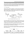
Thus, the real valued electrical OFDM signal is available after upconversion and
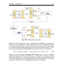
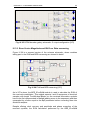
drives directly the e/o modulator. Figure II.17 shows the schematic designed by
Lowery and Armstrong in [P12] for one of the first direct detection optical OFDM
published simulations using VPI software, where the offset single sideband
technique (OSSB) was used. It dates from year 2007, and it has been the basis
of the system designed in this work.
36
FIBER-BASED OFDM TRANSMISSION SYSTEMS
Fig. II.17 DDO-OFDM Long-haul optical communication system [P12]
After the signal passes through fibre link with chromatic dispersion, the OFDM
signal can be approximated as
(II.17)
where
is the phase delay due to chromatic dispersion for the
subcarrier,
is the accumulated chromatic dispersion in unit of picoseconds
per picometer (ps/pm), is the centre frequency of O-OFDM spectrum, and c is
the speed of light. At the receiver, only one photodetector is used, which can be
modelled as the square law detector so the resultant photocurrent is
(II.18)
The first term is a DC component that can be easily filtered out. The second
term is the fundamental term consisting of linear OFDM subcarriers that are to
be retrieved. The third term is the second-order nonlinearity term that needs to
be removed.
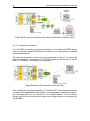
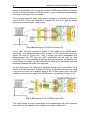
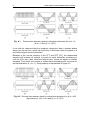
Those terms will be easily identified in the next set of figures, which shows the
contributions and results of the mixing products that appear at the receiver
when the optical carrier mixes with the optical subcarriers to regenerate the
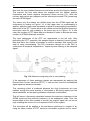
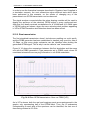
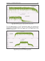
electrical OFDM signal. First, the received optical spectrum for an OSSB OOFDM transmission is depicted in Figure II.18, and then each of its components
are analyzed in Figures II.19, II.20 and II.21:
CHAPTER II – OPTICAL OFDM
37
Fig. II.18 Received optical spectrum [P13]
The OFDM subcarriers have a bandwidth
and there is a gap,
, between
the carrier and the subcarriers, which can be produced by RF upconversion of
the electrical OFDM signal or by zero padding at the input IFFT sequence, as
explained in Chapter I. The amplified spontaneous emission (ASE) inherent to
the laser is unpolarized and is band-limited by an optical filter, extending from
below the carrier to
above it, being present in both the lower and the
upper sideband zones.
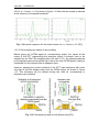
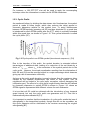
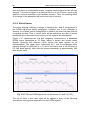
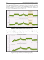
The useful components in the electrical spectra (that is, the OFDM subcarriers)
are the different terms which result from the mixing of the OFDM sideband and
the optical carrier. Figure II.19 shows the optical spectra of the contributions to
this mixing and the resulting electrical spectra after downconversion.
Fig. II.20 Useful components in the electrical spectra [P13]
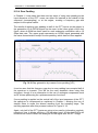
When a frequency guard band is used (
) all of the results of the
mixing products between OFDM subcarriers will fall out of band, not degrading
performance. This way, the unwanted out of band noise will be avoided:
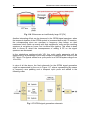
Fig. II.20 Unwanted out of band noise [P13]
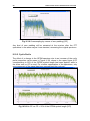
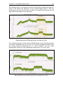
However, other undesired mixing products resulting from the square law
detection will fall inside the OFDM band. Those are called the unwanted inband
terms, and correspond to the products resulting from optical carrier x noise,
OFDM signal x noise and noise x noise, as depicted in Figure II.21. Noise from
both sidebands will be detected unless a narrow optical filter is used.
38
FIBER-BASED OFDM TRANSMISSION SYSTEMS
Fig. II.21 Unwanted inband terms [P13]
The single tap equalizer function in the OFDM receiver corrects for the
amplitude distortions caused by frequency roll-off of the components and the
phase distortions caused by CD and OFDM symbol timing offsets. It should be
taken into account that there may be other mixing products because of
nonlinearities in the system or I/Q imbalance in the transmitter.
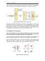
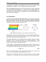
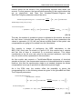
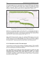
Figure II.22 represents a typical DD receiver used in optical OFDM, where the
optical and electrical spectrums before and after the photodetector are also
represented.
Fig. II.22 Direct detection at the receiver [P4]
It can be seen that the second-order intermodulation is located in the guard
band from DC to the OFDM signal bandwidth B, whereas the OFDM spectrum
spans from B to 2B. Then, the RF spectrum of the intermodulation does not
overlap with the OFDM signal, meaning that the intermodulation does not cause
detrimental effects after proper electrical filtering.
CHAPTER II – OPTICAL OFDM
39
Once photodetected, the electrical signal is downconverted to baseband in the
opposite way as it was done at the transmitter, before applying the FFT to
ideally recover the original subcarriers.
Thus, if the optical OFDM band is located close to the optical carrier in the
frequency domain, the intra mixing products are located in the same frequency
range as the electrical OFDM signal leading to performance degradation.
Taking all this into account, it can be said that the optical bandwidth
requirements for direct detection optical OFDM are determined both by the
OFDM band and the gap between the OFDM band and the optical carrier,
always omitting one optical sideband. Typically the width of gap is equal to the
width of the OFDM band in minimum.
II.5.2.2. Coherent Optical OFDM
Coherent optical OFDM (CO-OFDM) represents the best performance in
receiver sensitivity, spectral efficiency and robustness against polarization
dispersion, but it requires the highest complexity in the transmitter design.
There are two main advantages coming from the combination of coherent
optical communications and OFDM: OFDM brings coherent systems
computation efficiency and ease of channel and phase estimation, and the
coherent systems bring OFDM a much needed linearity in e/o upconversion and
o/e downconversion, since a linear transformation is the key goal for the OFDM
implementation. Moreover, there is no need to create a gap between the OFDM
signal and the DC component as in the DD receiver setups.
The principle of coherent OFDM is depicted in Figure II.23:
Fig. II.23 Principle of coherent OFDM receivers [P4]
In coherent OFDM systems, the optical carrier is not transmitted with the optical
OFDM signal, but generated locally by a laser. This makes this kind of system
to require less transmitted optical power than DD-OOFDM, though it is more
sensitive to phase noise.
As shown above, a local oscillator (LO) is mixed with the OFDM signal by
means of a 90º hybrid that performs the optical IQ detection. If both signals are
40
FIBER-BASED OFDM TRANSMISSION SYSTEMS
aligned in polarization, the mixing of the optical OFDM signal with the LO signal
results in the desired electrical OFDM signal. In case of orthogonal polarizations
there are no mixing products available.
There are two frequently used configurations regarding to coherent receivers for
optical OFDM. Those are depicted in Figures II.24 and II.25, and are called
homodyne and heterodyne, respectively.
Fig. II.24 Homodyne CO-OFDM receiver [P4]
In this case, the local oscillator is placed in the middle of the OFDM signal.
Essentially, this implementation is the reverse of the transmitter using the
optical IQ mixer in Figure II.18. Thus, it shares the same advantages and
disadvantages: the FFT size and ADC bandwidths can be used for data
modulation (if no oversampling is applied) and few electronic components are
used, though it requires two ADCs and the IQ MZM at the transmitter side has
three bias voltages that need to be adjusted.
On the other hand, the heterodyne reception setup can be considered as a
variant of the DD receiver in Figure II.22, where an electrical IQ mixer was used
to process the real and imaginary parts of the OFDM signal. Here, the local
oscillator is placed left or right of the OFDM signal, as depicted in Figure II.25:
Fig. II.25 Heterodyne CO-OFDM receiver [P4]
This setup shares the same advantages and disadvantages with the homodyne
one, so its use will depend on the chosen transmitter configuration.
CHAPTER II – OPTICAL OFDM
41
As explained in Chapter I, the electrical IQ mixer at the receiver can be
substituted by a larger FFT block to implement the required operations.
The optical bandwidth requirements for CO-OFDM are much lower compared to
DD optical OFDM because there is no need to transmit an optical carrier with
the required gap to the OFDM band in addition to the modulated subcarriers.
This leads to a spectral efficiency of nearly twice the one in DD-OFDM for any
type of subcarrier modulation.
II.6. Equalization
In order to obtain an OFDM signal without errors at the receiver, the use of
cyclic prefix is essential. This will eliminate ISI when a temporal dispersion
affects the channel. However, the effect of chromatic dispersion causes the
information symbols to still be affected by amplitude and phase changes when
arriving to the receiver, as shown in Figure II.26:
Fig. II.26 Phase distortions on the received constellation [P4]
Consequently, an N-level equalizing stage has to be introduced right after the
FFT operation at the receiver in order to correct the phase and amplitude levels,
where N is the number of received subcarriers.
The design parameters for this stage should be obtained through a channel
estimation, which is usually performed with training sequences. These
sequences are added by using pilot subcarriers in each OFDM symbol, so the
channel transfer function can be approximated.
As the design of training sequences is beyond the scope of this work, the
required phase compensation for each OFDM symbol will be calculated based
on the dispersion model suffered by each subcarrier (see section II.X):
(II.19)
Where L is the fibre length, is the subcarrier frequency, and
term order of the signal phase delay approximation in (II.7).
is the second
However, this equalization will be not enough to obtain the ideal received
constellation, as a constant phase shift will still affect the received symbols due
42
FIBER-BASED OFDM TRANSMISSION SYSTEMS
to the choice of the reference frequency for the fibre. This issue will be dealt
with in section IV.X.
CHAPTER III – VPI DEMOS
43
CHAPTER III - VPI DEMOS
Virtual Photonics Integrated (VPI) is a powerful tool that allows to simulate a
wide range of optical transmission designs, giving the possibility to create
multiple configurations for a given transmission scenario. Specifically, the
simulations described in this chapter are going to be performed by means of the
VPI Transmission Maker application, though it will be simply referred as VPI
during this work.
VPI contains two demonstration scenarios which are very interesting regarding
this work’s purposes. Those are the OFDM Generation and Detection demo
(Optical Systems Demos/Modulation Multilevel/) and the OFDM for Long-Haul
Transmission demo (Optical Systems Demos/Long Haul/).
These demos are going to be described in this chapter in order to get an idea of
how to implement an optical OFDM transmission on a simulation environment.
The first demo simply deals with the generation and detection of an electrical
OFDM signal, so no optical transmission is considered at all, while in the
second one some of the concepts explained in the previous chapter are applied
so the signal can be optically modulated, transmitted through optical fibre and
detected at the receiver end, where the transmission quality is assessed in
presence of various transmission impairments.
The simulation results presented in this chapter, as well as the ones in Chapter
IV, have been displayed by means of the VPI Photonics Analyzer tool, which is
automatically executed after the simulation is run when using in the setup any of
the analyzer modules provided by VPI.
In order to understand VPI’s simulation environment, Section III.1 describes its
basic structure and the most important settings to take into account when
creating a simulation. For more information about it, see the VPI Transmission
Maker user’s manual in [W6].
III.1. VPI Transmission Maker as a simulation tool
III.1.1. Graphical User Interface
When starting VPI, the basic screen layout is similar to other simulation
programs based on interconnection of modules to create, design and simulate
the operational characteristics of determined systems.
Figure III.1 shows VPI’s graphical user interface (GUI), where some numbers
have been added in order to identify each of the parts which are going to be
mentioned during this section.
44
FIBER-BASED OFDM TRANSMISSION SYSTEMS
Fig. III.1 VPI Graphical User Interface [VPI]
The highlighted toolbar menu in (1) has the same function as in the most part of
software programs menu, as any available action offered by VPI can be
executed from here: creating and editing a simulation scenario, preferences
configuration, visualization of parameters, etc.
In (2), the most typically used options from the toolbar menu are available as
shortcuts, with functions such as creating a new scenario, saving, zooming,
executing or stopping the simulation, etc.
When a new file is created (by clicking FileNew in the toolbar menu or using
the corresponding shortcut), an empty schematic as the one in (3) appears. In
order to add already existing modules, the Quick Find or Search tabs in (4) can
be selected to look for them.
If the name of the desired module is not known, the Tree tab in (4) should be
selected, and by pressing the TC Modules button in (5), all the available
modules can be accessed by categories.
Another interesting option is offered by the Optical Systems Demos button (6),
which displays the category panel (7) containing all the demonstration
simulations offered by VPI. By selecting a category, another panel containing
CHAPTER III – VPI DEMOS
45
the corresponding demos appears. In Figure III.1, this is indicated by (8), where
the OFDM Generation and Detection demo is selected (highlighted in blue).
Finally, the schematic’s Package Explorer is highlighted in (9), consisting of a
folder browse panel (9a) and a contents panel (9b). The folder panel is used to
attach and store any data to be used by the schematic. The contents panel
shows the files and documents contained in the currently selected folder in the
folder panel.
III.1.2. Simulation hierarchies
VPI is hierarchically organised. This allows an easier management of the
modules taking part in a simulation, as they can be treated independently or as
a group when necessary.
Figure III.2 shows the three levels in which modules can be classified: those are
the universe, galaxy and star. As it can be deduced by their names, the star
represents the lowest level of the simulation interface, the galaxy belongs to the
second level and the universe is the third and highest level.
Fig.III.2 VPI hierarchy [VPI manual]
A star represents a unique module with a specific function which can’t be
subdivided into other modules. Thus, a galaxy can be described as a second
level module formed by a set of interconnected stars (or even other galaxies). In
order to be implemented on a universe, a galaxy must contain at least one input
or output port (see Figure III.2).
46
FIBER-BASED OFDM TRANSMISSION SYSTEMS
The universe is the only module that can be executed by the user. It represents
the whole simulation scenario, and it can consist of a combination of
interconnected stars and galaxies. From a universe point of view, a galaxy acts
as another unique module and the stars inside this galaxy can’t be seen from
the main schematic. However, the galaxy schematic can be displayed by rightclicking on it from the universe schematic and selecting the Look inside option.
III.1.3. Simulation parameters
When executing a simulation, any star, galaxy or universe belonging to it will
operate according to certain parameters. The value for these parameters can
be changed from the corresponding Parameter editor window (PEW). Figure
III.3 is an example of a PEW corresponding to a laser module:
Fig. III.3 Parameter editor window (PEW) of a VPI laser module [VPI]
The Parameter editor of a module can be accessed by right-clicking on it and
selecting the Edit Parameters option, or just by double-clicking on the module.
In the case of a universe or when being inside a galaxy, the same operations
can be done by clicking on the background.
Because of the hierarchical organization, any parameter which is shared by
more than one module, even if it is used in different levels, will take the value of
the highest level in which it is used.
For instance, consider a transmission system where the scenario itself is a
universe containing various galaxies (say one coder and one decoder), and
these galaxies contain at the same time other modules (stars) to implement its
respective functions. If, for example, the roll-off parameter of a pulse shaping
filter acting as a star inside both the coder and decoder modules is defined in
the universe PEW, any change in its value from this level will be applied to both
modules belonging to the galaxies.
CHAPTER III – VPI DEMOS
47
On the other hand, if the value of this parameter is changed directly from the
pulse shaping star inside the coder, it will only affect this module, leaving the
one inside the decoder untouched.
This feature will be used in the customized simulations presented in the next
chapter when a simultaneous change is desired for any parameter of both the
OFDM coder and decoder modules.
Thus, two types of parameters can be defined: global parameters, which affect
to all the modules within a simulation (lower levels included), and the specific
ones, belonging to a single module.
III.1.3.1. VPI global parameters
Besides the parameters that can be defined by the user to be used by all the
modules in a simulation, VPI provides a set of already defined global
parameters, which are very important for the correct and efficient operation of
the simulator. The most relevant for this work’s purpose are:

TimeWindow: this parameter sets the period in which a block of data is
represented. This time will inevitably fix the spectral resolution of the
simulated signals setting, i.e., the resolution of spectral displays.

LogicalInformation: This is a tool used by VPI to send information
between modules within the same simulation. It removes the need for
sneak wires between the transmitters and some modules such as BER
Estimators, Clock Recovery modules and the Channel Analyzer.

SampleRateDefault: it specifies the sampling frequency when working in
Block Mode. It is defined as the number of samples taken by second
and determines the maximum frequency that can be simulated.

BitRateDefault: it defines the transmission bit rate by setting the BitRate
parameter of emitters, bit generators, etc. to BitRateDefault.
III.1.3.2. Restrictions on Global Parameters
As VPI works with the FFT algorithm, when working with periodic signals a
series of restrictions have to be considered. First, the number of samples by
Time Window has to be a power of two. This condition sets a limitation when
selecting the Time Window and the Sample Rate, as expressed in (III.1):
(III.1)
Additionally, the time resolution has to be considered, given by (III.2). This will
determine the maximum allowed simulation frequency given by (III.3).
(III.2)
48
FIBER-BASED OFDM TRANSMISSION SYSTEMS
(III.3)
Finally, the frequency resolution will be given by Expression (III.4). A proper
selection of the Time Window is required in order to obtain a correct signal
frequency spectrum. At the same time, the Time Window determines the
minimum allowed simulation frequency given by (III.5), since the period of the
simulated signal T always has to be smaller than the Time Window.
(III.4)
(III.5)
III.1.4. Custom modules
III.1.4.1. Creating and adding galaxies
To create a new galaxy, the user has to click on the File - New option in the
toolbar menu, and a new schematic will appear. At first it will be considered as a
universe, though it will automatically saved as a galaxy when input and output
ports are used in the schematic. These ports can be found in the Tree tab of the
GUI, pressing the TC Modules button and selecting the Wiring Tools category.
To add a customized galaxy module, the option Insert – Add module in the tool
bar allows loading it into a universe or galaxy schematic by just selecting them
from the corresponding location (if known). VPI modules can also be loaded in
this way.
When adding an already existing galaxy to a schematic, the user can choose
between inserting a copy or a link of the mentioned galaxy. Figure III.4 shows
the VPI message appearing in this case for a galaxy named RF_Upconversion:
Fig. III.4 Copy or link to an already existing galaxy [VPI]
CHAPTER III – VPI DEMOS
49
If the Copy option is selected, VPI will copy the entire galaxy to the Resources
folder in the schematic’s Package Explorer, and any change on the galaxy will
not be applied to the original one. On the other hand, selecting the Link option
will cause that the galaxy is executed from the original location, so any
modification will be saved, affecting it even when it is added to other scenarios.
III.1.4.2. Creating and linking parameters
Although any value of a star module parameter can be changed when running a
simulation, the parameter properties cannot be edited. Thus, new parameters
can only be created for either galaxies or universes. This can be done by
accessing the PEW and clicking the Create parameter button, as shown in
Figure III.5:
Fig. III.5 Create parameter button [VPI]
After clicking the button, a menu in which the parameter settings can be
configured will appear, as shown in Figure III.6:
Fig. III.6 New parameter settings [VPI]
50
FIBER-BASED OFDM TRANSMISSION SYSTEMS
In this case, a new parameter is going to be created in a category called RF
galaxies. New categories can be created for a better organization of the
parameters, appearing as expandable folders as in Figure III.5. The Create
category button in the same figure (a yellow folder icon to the left of the Create
parameter button) allows to create a new category. To insert a parameter into a
category, it just has to be dragged into the corresponding folder.
Any parameter can be shared by modules belonging to different simulation
levels as long as it has the same name for every module containing it.
When creating a new simulation scenario where modules of different levels will
share some parameters, the usual (and easier) procedure is to create
parameters in the lower level and then expand them to the upper levels.
This expansion of a parameter is done by right clicking on the created
parameter and selecting the Create Schematic Parameter option, as shown in
Figure III.7. This way, the parameter and its corresponding category will be
automatically created in the upper level with the same settings.
Fig. III.7 Create Schematic Parameter option [VPI]
In order to make the parameters management easier, the highest level
parameter should be the only one indicating the value used for the simulation,
while the lower level ones should just indicate its name in the Value field.
However, this field can be given another value if a module belonging to a lower
level has to work with other characteristics than those of the higher level ones.
CHAPTER III – VPI DEMOS
51
III.1.4.3. Cosimulation
Cosimulation is a technique in which some part of the simulation is handled by
an application other than the VPI Transmission Maker simulator. It allows three
different programming languages to interact with VPI: Matlab, Phyton and
C/C++. This technique has played a very prominent role in this Master Thesis,
as it has been used to build a complete optical OFDM simulation tool by the
combination of the Matlab programming for the OFDM coding and decoding and
VPI modules for the simulation of the RF and optical paths.
The main module to carry out the cosimulation is called the CosimInterface
module, and it is represented in Figure III.8:
Fig. III.8 CosimInterface module [VPI]
To execute a programming code, the code file must be attached to the Input
folder of the schematic containing the CosimInterface module, and its main
function (which name must be the same as the code file name) has to be
indicated in the RunCommand parameter value of the module’s Parameter
editor. This process is shown in Figure III.9 for the case of a Matlab code.
Fig. III.9 Main code function indicated in the RunCommand parameter [VPI]
In this case, the variable x will take the output value of the function
ofdm_decoder_simu. Note that this name is the same for the Matlab file
attached to the Input folder of the schematic.
52
FIBER-BASED OFDM TRANSMISSION SYSTEMS
VPI provides other cosimulation modules which act as inputs and outputs of the
CosimInterface module. Those are used to indicate the type of data that is
going to be inserted and extracted from the cosimulation, allowing the use of
electrical or optical signals, floating numbers, complex numbers, etc. As an
example, Figure III.10 shows an interconnection of a CosimInterface module
with one optical input (CosimInputOpt) and one optical output
(CosimOutputOpt).
Fig. III.10 CosimInterface interconnection for optical signal processing [VPI]
This way, an optical signal generated with VPI modules could be processed by
one of the mentioned programming software, which allows the user to modify
the signal parameters and extract them in a customized way.
The CosimInterface module will be the key to the performed simulations in the
next chapter, acting as an interface for VPI to access the Matlab codes
programmed for this work, which contain the OFDM coder and decoder
functions.
III.2. OFDM Generation and Detection Demo
III.2.1. General schematic
The next figure shows the universe schematic view for the OFDM Generation
and Detection demo provided by VPI in Optical Systems Demos/Modulation
Multilevel in the left panel labels.
Fig. III.11 OFDM Generation and Detection [VPI]
CHAPTER III – VPI DEMOS
53
The goal of this section (as well as the following one) is to learn from each
demo towards a new definition of a simulation setup for optical OFDM systems.
In this case, a complex-baseband OFDM signal is generated in an OFDM coder
(1) connected to the OFDM decoder (5) by means of VPI wires, so the received
signal is directly detected without any transmission channel between transceiver
and receiver. This means an ideal channel transmission.
Also, two visualizer modules (4,8) can be seen, which function is to extract the
relevant results from the simulation. Before the first visualizer (on the left in the
figure) two pulse shaping modules (3) will generate a Nyquist response from an
incoming electrical impulse.
The transmission is initiated in a PRBS or pseudo random bit sequence
generator (1). According to the module’s definition in the Reference Manual
(right-click on the module and select the Help option) the output of this module
is a sequence of random integer numbers, forming a vector of size
TimeWindow*Bitrate that will be fed to the coder. See the Reference Manual in
[W6] for more details about the characteristics of this random sequence and the
available types of sequence to select from the PRBS Parameter editor window.
Despite not being able to see the internal structure of the OFDM coder galaxy,
its operation principles can be guessed based on the acquired concepts during
the investigation prior to the realization of this chapter.
For an M-QAM modulation, an OFDM coder in its simpler form (omitting zero
padding and cyclic prefix overheads) would first pack the bit sequence coming
from the PRBS into
sets, assigning one QAM symbol to each set. Thus,
the parameter BitsPerSymbolQAM from the schematic’s PEW allows changing
the M factor for the QAM modulation, as shown in Figure III.12:
Fig. III.12 Configurable parameters from the universe schematic [VPI]
54
FIBER-BASED OFDM TRANSMISSION SYSTEMS
Once the bits have been converted to QAM symbols, the coder will perform an
IFFT operation for each N symbols forming an OFDM symbol, resulting in a
sequence of floating numbers of size TimeWindow*BitRate/BitsPerSymbolQAM,
meaning a reduction of a factor
for the sequence length.
By checking the Reference Manual for the coder module, it can be seen that its
two outputs represent electrical samples of the real and imaginary components
of the complex OFDM symbols. After several tests and careful readings of the
available documentation on the subject, it has been deduced that an
upsampling operation is carried on the sequence at the output of the IFFT stage
in order to be converted into electrical samples.
Another key to the above conclusion lies on the UnPackBlockEl (6) and
Downsample (7) modules used to convert the electrical samples at the output of
the decoder into numerical samples, as it will be seen later.
Thus, the original sequence length (TimeWindow*BitRate) is recovered to
match the sampling rate required by VPI, obtaining at the output the electrical
samples that represent the analogue OFDM signal.
Note that the OFDM coder has two outputs which are not only connected to the
decoder, but also processed by the PulseRaisedCosQAM modules (3) serving
as pulse shaping filters. As it was explained in Chapter I, the most suitable
impulse response for an OFDM signal is the square-root raised cosine
approach, so the squareRootRaisedCosine option should be selected as the
Nyquist response parameter for these blocks.
Once this type of filtering is applied, both parts of the signal are ready to be
represented, so the SignalAnalyzer module (4) is used as an interface to the
VPI Photonics Analyzer tool, where the signal will be displayed. The results of
this representation will be described in Section III.2.4.
At the receiver side, the decoder module performs the opposite operations
carried on in the coder module, providing the electrical samples representing
the real and imaginary parts of the decoded complex information symbols.
These parts are going to be fed to another kind of analyzer (8), which will plot
the received constellation based on the received information symbols.
But before that, as both inputs and outputs of the decoder belong to the
electrical type, the electrical samples of each branch have to be transformed
into floating-type values that will represent samples of the electrical OFDM
signal. This function is carried on by the UnpackBlockEl modules, as it can be
seen in (6) from Figure III.11.
Once the electrical signal is sampled, the number of samples needs to be
reduced so just the correct amount of information symbols is represented on the
constellation diagram.
CHAPTER III – VPI DEMOS
55
As it was explained in the coder case, this is because VPI needs the number of
samples of the original bit sequence to be at least equal to the number of
samples to be represented as an electrical signal. As the coder internal
sequence is organized in symbols (not in bits), it is supposed that this sequence
is internally upsampled so it can be correctly processed by the software.
Thus, two DownSample blocks (7) are used to provide the exact amount of
information symbols to be represented by the next module. The downsampling
factor indicated in the Parameter editor of these blocks is set to:
(III.6)
As the SampleRateDefault parameter is set to
for this demo (in order to have a frequency simulation window
that is 4 times larger than the required optical bandwidth of the optical OFDM
signal), the downsampling factor (and also the internal upsampling factor of the
coder) will be 4 for any type of subcarrier modulation and bitrate.
The constellation diagram is plotted by the NumericalAnalyzer2D module (8),
which also acts as an interface to the VPI Photonics Analyzer tool.
III.2.2. Coder and decoder parameters
Figure III.13 shows the OFDM coder parameters that can be changed from its
PEW. The same parameters are shared by the decoder module, which
performs the same functions as the coder in the reverse order.
Fig. III.13 Coder (decoder) parameters [VPI]
Three of the parameters are shared with those of the universe schematic:
SampleRate, BitRate and BitsPerSymbolQAM. Thus, any change in their values
will not have any effect on the simulation unless it is done in the upper level.
The rest of the parameters (all of them belonging to the Physical category) are:
56
FIBER-BASED OFDM TRANSMISSION SYSTEMS

OFDMType: This parameter allows to choose between three different
modulation types: OFDM, where no zero padding is used; DMT (Discrete
Multi Tone), where half of the inputs of the IFFT are the complex
conjugate of the other half so a real OFDM signal is created at the
transmitter output, as explained in Annex 1; and Zero Padding. The latter
technique is used to create a gap between the OFDM signal and the DC
component, as described in Chapter I.

Coding: Select either mQAM or mPSK coding to modulate subcarriers.

NumberOfCarriers: Number of subcarriers taking part on the modulation.
If the Zero Padding technique is used, only half of the subcarriers will be
used to encode the signal, meaning a loss of 50% of the effective data
rate. The same will happen with the DMT modulation type.

CyclicPrefix: The length of the cyclic prefix relative to the symbol length,
ranging from 0.0 to 1.

QuantizeOutputValues: If this parameter is set to Yes, the output values
of the coder are quantized. The number of quantization levels and the
higher quantization level should be indicated afterwards. This technique
is useful to simulate the effect of a DAC and also to clip the signal when
it exceeds a determined level.
If any of these parameter values needs to be changed, it should be done in both
coder and decoder. Thus, one way to achieve an easier configuration of the
schematic would be to create schematic parameters as explained in the last
section, so just a single parameter change is required to affect both modules.
However, the main disadvantage of the coder and decoder modules is that all
the performed operations are internal, meaning that they don’t allow looking
inside them for a detailed analysis of the working procedures. Despite some
basic concepts are explained in the Reference Manual, it can be said that those
modules are quite rigid in terms of showing the structure and organization of the
internal operations carried on inside them.
The problems indicated in the last paragraphs have been the cause of a need
for new coding and decoding tools where every operation can be checked and
even modified. Hence, custom coder and decoder modules have been
developed to implement the same operations as those of VPI, as it will be seen
in Chapter IV.
III.2.3. Simulation results
When running the simulation, two graphs are going to be shown in the Analyzer
tool: the electrical signal spectrum and the received constellation diagram. As
the signal transmission is done over an ideal channel, no dispersion will appear
on the constellation diagram, so for case of 4-QAM modulation (mQAM coding
with BitsPerSymbolQAM parameter set to 2) it will be displayed as 4 points
forming a square, each of them representing one information symbol.
CHAPTER III – VPI DEMOS
57
This case is represented in Figure III.14 for the OFDM type of coding. The
parameters for this simulation are:






BitRateDefault = 10 Gbps
BitsPerSymbolQAM = 2
SampleRateDefault = 4/BitsPerSymbolQAM*10e9 = 2*BitRateDefault
TimeWindow = BitsPerSymbolQAM*4*1024/10e9 = 8192/BitRateDefault
NumberOfCarriers = 16
CyclicPrefix = 0.2
Moreover, the pulse shaping filter has been set with the following parameters:


RollOff = 0.18
SymbolRate = BitRateDefault/BitsPerSymbolQAM
Fig. III.14 4-QAM received constellation diagram [VPI]
Apart from the 4 possible information symbols, at least one symbol is also
represented in the centre of the diagram (circle in [0,0]). This is because VPI
organizes the sequence to be transmitted by first calculating the required
information symbols according to the bits per symbol and cyclic prefix
parameters, discarding a number of bits from the original sequence which will
be occupied by the bits representing the required cyclic prefix quantity.
If the resulting number of OFDM symbols does not cover the whole sequence,
VPI fills it with zeros to compensate for any differences between the effective
and transmitted data rates, and symbols in [0,0] are represented as long as
those padded zeros are not previously extracted. This is another point to be
improved by the upcoming custom simulations.
The transmitted signal spectrum will be represented by means of a signal
analyzer for both the real and imaginary components of the OFDM signal. As
negative frequencies do not exist for a real system, a complex-baseband OFDM
signal like the one which is being generated will be represented as in Figure
58
FIBER-BASED OFDM TRANSMISSION SYSTEMS
III.15, where the real and imaginary parts (in green and blue, respectively) are
superimposed:
Fig. III.15 Superimposed OFDM signal spectrum [VPI]
Because of this superimposition of the signal, just half of the OFDM bandwidth
will be represented. The OFDM signal bandwidth is calculated as the
transmission bitrate divided by the number of bits per symbol, so the expected
electrical bandwidth for this case should be 2.5 GHz, as just half of the
spectrum is depicted.
The exceeding bandwidth of nearly 300 MHz that can be identified in Figure
III.15 is due to the roll-off factor of the filter applied in the pulse shaping module.
Two more simulation results are shown in Figures III.16 and III.17, representing
the transmitted electrical spectrum and received constellation diagram for the
other two possible modulation types: Zero Padding and DMT. The parameters
used for these simulations are the same as before.
Fig. III.16 Zero Padding modulation [VPI]
CHAPTER III – VPI DEMOS
59
For the Zero Padding simulation, zeros have been added at both edges of the
IFFT input sequence, as said before. The resulting gap represents nearly half of
the ideal signal bandwidth (that is, 2.5 GHz), as it can be seen in Figure III.16.
Again, the received constellation is ideal, though just half of the received
information symbols are being represented due to the use of zero padding for
half of the IFFT input sequence. This could be appreciated in a non-ideal
channel transmission where dispersion would separate the received symbols in
the constellation diagram. The zero padding observed could be used in
accordance with the following section as a technique to avoid the RF
upconversion stage and yet provide the required guard band for the use of
conventional IM/DD optical transmission systems.
The spectrum of the transmitted signal for a DMT modulation can be seen in
Figure III.17, where only the real part of the signal is represented, while the
imaginary component is zero. It can be seen how the use of the complex
conjugate in half of the input IFFT sequence allows the elimination of the
negative band at a cost of reduced bitrate efficiency (see Annex A).
Fig. III.17 DMT modulation [VPI]
Other parameters such as cyclic prefix or bits per symbol will be changed in the
simulations performed with custom modules in Chapter IV, so it can be seen the
effect on both the signal spectrum and the received constellation.
60
FIBER-BASED OFDM TRANSMISSION SYSTEMS
III.3. OFDM for Long-Haul Transmission Demo
III.3.1. General schematic
In this simulation scenario, the OFDM signal is generated and detected as in
the last demo, though two major changes are applied: those are RF frequency
up/downconversion and optical signal modulation and demodulation. Also, the
transmission is done over a 1000 km optical fibre link. Figure III.18 shows the
universe schematic for the simulation, which can be found in the left panel
labels of VPI-TM in: Optical Systems Demos/Long Haul/.
Fig. III.18 Universe of the OFDM for Long-Haul Transmission demo [VPI]
The OFDM coder module is now placed inside an OFDM transmitter galaxy (left
bottom in the figure), where a frequency upconversion is applied to the signal
after being generated, as it will be seen later by looking inside the galaxy. This
technique was described in section I.3.1, and is used to create a gap between
the OFDM signal spectrum and the electrical DC component, so the unwanted
mixing products appearing due to the IM modulation and direct detection (DD)
method used fall outside the OFDM bandwidth.
For a 10 Gbps bitrate with 4-QAM modulation, an OFDM bandwidth of 5 GHz is
required and thus an RF carrier of 7.5 GHz is used to generate a 5 GHz gap.
This will be seen at the simulation results section at the end of the chapter.
Once the signal is upconverted to an RF frequency, it is optically modulated by
a Mach-Zehnder modulator (MZM), giving rise to the RF upconversion based on
Intensity Modulation configuration described in section II.5.1.1 (Figure II.15).
Then, the optical signal is filtered to suppress the lower sideband (see section
II.3 to see why optical single sideband is needed), and transmitted through a
fibre link consisting of a loop circuit where the signal covers 100 km with
amplification and filtering stages for each loop.
At the receiver side, a single photodiode is used in DD configuration, and the
resulting photocurrent is fed to the OFDM receiver galaxy, which holds the
CHAPTER III – VPI DEMOS
61
OFDM decoder module inside. The frequency downconversion is also applied
within this module to recover the original baseband OFDM signal, just before
the decoding functions.
Three kinds of output results are provided by this demo by using the
corresponding visualizer modules:

Received constellation: the required numerical analyzer is located inside
the receiver galaxy

Spectrum at the receiver input (right bottom visualizer in Figure III.18)

The error vector magnitude (EVM) at the receiver output. This value can
be considered as an indicator of how far the received constellation points
are from their ideal location.
The 1D numerical analyzer in charge of calculating the EVM will obtain
information about the emitted sequence by means of the virtual optical channel
feature of VPI. This means that the correct ChannelLabel value should be
assigned to the module providing this information, which is placed inside the
receiver galaxy (see section III.3.3).
The schematic parameters of this demo are the same as those of the OFDM
Generation and Detection demo’s universe parameters in Figure III.12, allowing
the change of global parameters and the number of bits used to represent one
QAM symbol.
However, the galaxies that represent the OFDM modulator and demodulator
have a much more complicated structure, as described in the following sections:
III.3.2. Inside the OFDM transmitter module
As it can be seen from Figure III.19, the structure of the OFDM coding and
pulse shaping functions is identical to the one used in the OFDM Generation
and Detection demo (see Figure III.11).
Fig. III.19 Schematic of the OFDM transmitter module [VPI]
62
FIBER-BASED OFDM TRANSMISSION SYSTEMS
However, this time an RF upconversion stage is added to convert the baseband
OFDM signal into a passband centred at an RF frequency, in this case 7.5 GHz.
This is simply done by multiplying both the real and imaginary components of
the OFDM signal (that is, inphase and quadrature) by an electrical sine
waveform provided by the FuncSineEl module. A 90º constant phase shift will
be applied to the quadrature component, and both parts are added to form the
upconverted electrical OFDM signal described in expression (I.6). This
operation is performed by the PhaseShiftEl module, which connects the sine
function generator to the lower branch of the schematic.
Once the final electrical OFDM signal is obtained, it is added to the
LogicAddChannel module along with the original PRBS sequence. As it was
said for the definition of the LogicalInformation global parameter, this module is
used to send information between modules within the same simulation. For
instance, the EVM will be calculated at the receiver without the need of any
wires between it and the OFDM transmitter galaxy.
The available parameters of the transmitter module are shown in Figure III.20,
where some new categories have been defined in order to achieve a better
organization. Two of them are important to understand the simulation, so they
are described below.
Fig. III.20 OFDM transmitter parameters [VPI]

ChannelLabel: indicates the name of the logical channel. It must be the
same for all of the modules using the original sequence that was added
to the LogicAddChannel module.

CarrierFrequency: Indicates the RF frequency at which the baseband
OFDM signal will be upconverted. This value is set from the schematic
parameter, so it will also affect the RF downconversion stage of the
OFDM receiver galaxy.
CHAPTER III – VPI DEMOS
63
The main category in this PEW is the Physical category, which contains the
QAM-OFDM Signal subcategory. At the same time, QAM-OFDM Signal is
divided into other subcategories, such as the PRBS generator, DAC, RF and
Filter. As these smaller categories are declared as galaxy parameters, they can
be edited from the main schematic by double-clicking on the module, without
the need to look inside and change them on the corresponding module. The
same can be applied to the OFDM receiver galaxy.
III.3.3. Inside the OFDM receiver module
Once again, the OFDM receiver module will perform the same operations as the
transmitter in a reversed order. First of all the signal is downconverted by
multiplying it by the same RF frequency as before and applying a 90º phase
shift to the quadrature component, as shown in Figure III.21:
Fig. III.21 Schematic of the OFDM receiver module [VPI]
After that, both components pass through a pulse shaping filter and the
resulting electrical signal is fed to the OFDM decoder module, which provides
the decoded versions of the inphase and quadrature components.
The constellation diagram representation is done in a similar way as in the
OFDM Generation and Detection demo, though this time another function is
used between the decoder and the signal analyzer: two switches are connected
to a rectangular pulse generator (lower module in the figure).
This modification is used to extract the redundant information inside the
sequence, which was mentioned before. The rectangular pulse indicates the
period of time in which the switches allow the signal to flow as an input to the
signal analyzer module. The rest of time, any sequence coming from the
decoder is going to be discarded. This way, only the received information
symbols are going to be represented in the constellation diagram, omitting the
padded zeros used to compensate for any differences between the effective
and transmitted data rates.
64
FIBER-BASED OFDM TRANSMISSION SYSTEMS
The decoded OFDM sequence is also connected to another module (on the
right edge of the image). This module is called BER_El-mQAM, and its function
is to estimate the Symbol Error Rate (SER) and/or the EVM of an electrical
mQAM signal, taking I and Q electrical signals as inputs. The module
automatically performs clock recovery, amplitude and phase correction of the
received constellation. Thus, it will be able to perform these calculations as long
as its ChannelLabel parameter indicates the right logical channel name.
The following figure shows those parameters of the OFDM receiver module
which have not appeared until now:
Fig. III.22 OFDM receiver parameters [VPI]
The EVM-BER and Analyzer categories deal with the representation settings for
the EVM/SER and the received constellation, respectively. Thus, the
parameters indicated in these categories are going to be applied on the
BER_El-mQAM and signal analyzer modules.
The Equalization category (if the Equalization parameter is set to Yes) allows
the compensation of the chromatic dispersion suffered by the OFDM signal
during the optical channel transmission. The amplitude and phase coefficients
to be used have to be written as values in the corresponding parameters in
order to obtain the desired results. This should improve the EVM measure, as
well as achieving a proper constellation representation with less dispersion
between points (as shown in section III.3.5).
The equalizer coefficients for this demo are shown in Figure III.23, where
Matlab has been used to represent the applied phase equalization array (in
radians) for the 64 modulated subcarriers:
CHAPTER III – VPI DEMOS
65
Fig. III.23 Phase equalization curve [VPI]
It is thought that these coefficients have been experimentally extracted from a
training sequence after identifying the optical channel properties and are only
valid for the specific settings in the demo. If, for instance, the length of fibre, the
bit rate or the QAM levels are changed, a different sequence for the equalizer
must be used, which is not provided by the demo.
It will be seen that the custom simulations use a very similar equalizer shape
that comes from the simplified fibre model in which chromatic dispersion is
considered as the only relevant effect.
III.3.4. Optical channel path
The optical channel path is composed by an optical modulation stage, the fibre
link and a photodiode in direct detection configuration at the receiver.
Figure III.24 shows the optical modulation stage, where the two inputs of the
MZM correspond to its driver (connected to OFDM coder output) and a laser at
continuous wave (CW) mode.
Fig. III.24 Optical modulation stage [VPI]
66
FIBER-BASED OFDM TRANSMISSION SYSTEMS
The driver basically sets the optical modulation index relative to the half-wave
voltage of the MZM. Since the used MZM module is set by default at the
quadrature point (QP), the bias is set to 0.
The laser operating at CW provides the optical carrier to be modulated, and its
most relevant parameters are:



Emission frequency: 193.12 THz.
Average power: 5 mW
Linewidth: 1 MHz
Meaning that the laser operates at 3rd window, and thus the dispersion
coefficient of the optical fibre has to be set accordingly. A random noise is
generated in the laser, where the maximum allowed spectral density variation
within the noise bandwidth is set to 3 dB.
An optical filter is then used to suppress the lower sideband resulting from the
optical modulation. The used filter is of Gaussian type, centred at
,
where
is the optical carrier frequency (193.12 THz) and
is the electrical
carrier frequency at which the electrical OFDM band was upconverted (7.5
GHz). The filter bandwidth is set to 18 GHz.
As it can be seen from Figure III.18, the fibre link is composed of a loop where a
universal fibre module simulates the wideband nonlinear signal transmission
over optical fibre. After the fibre span, the signal goes through amplifying and
filtering stages to compensate for attenuation. The number of loops of the link is
set to 10, so for a fibre length of 100 km (default) the transmission distance will
be 1000 km.
The most important parameters of the fibre for this simulation are the ones
belonging to the Physical category, as represented in Figure III.25:
Fig. III.25 Optical fibre physical parameters [VPI]
The used attenuation and chromatic dispersion coefficient (
) are
rd
typical values for a transmission in 3 window. The rest of values are set to
default.
CHAPTER III – VPI DEMOS
67
Another important parameter to take into account is the ReferenceFrequency.
This frequency is where the dispersion characteristic of the fibre is centred. It
means that the optical group delay is considered zero at the specific frequency,
and therefore the waveforms in that subcarrier frequency are the ones at the
beginning of the time sequence at the receiver end.
Since the dispersion coefficient D (derivative of the group delay against
wavelength) in 3rd window is positive, the lower frequencies will arrive later
(after the reception window time has started) and higher frequencies will arrive
sooner (before the reception window time has started). This will be an important
concept to bear in mind for the correct choice of this reference frequency in the
simulations.
It is interesting to see that this reference frequency is set in the demos equal to
the sum of the optical carrier and the RF carrier, just at the optical frequency
where the OFDM spectrum is centred. The analysis about how and why to
choose the reference frequency precisely equal to that value and the derived
implications is carried out in section IV.3.4.
At the receiver, after DD and decoding, chromatic dispersion is compensated by
correcting the phase of each sub-carrier separately. The equalized phase
offsets correspond to the relative accumulated dispersion values experienced
by each sub-carrier during its transmission through optical fibre.
III.3.5. Simulation results
A list of the parameters used for this demo can be found below. These will be
the basis from where the simulations in the following chapter have been done. If
different values for any of these parameters are used, it will be explicitly stated.








BitRateDefault = 10e9 bps
TimeWindow = 8*1024/BitRateDefault seconds
SampleRateDefault = 4*BitRateDefault samples/second
BitsPerSymbolQAM = 2
NumberOfCarriers = 64
CyclicPrefix = 0.2
CarrierFrequency = 7.5 GHz
Reference frequency = 193.1 THz + CarrierFrequency
As the equalization coefficients represented in Figure III.23 are only calculated
for the dispersion parameters shown in Figure III.24 in a 1000 km transmission
distance (10 loops), any change in the fibre Physical parameters will distort the
form of the received constellation.
With this, once the simulation is executed, the VPI Photonics Analyzer tool will
display the received optical spectrum, the received constellation diagram and its
corresponding EVM.
68
FIBER-BASED OFDM TRANSMISSION SYSTEMS
The received optical spectrum is plotted just after the fibre link, before the signal
is detected by the photodiode. The result is shown in Figure III.26:
Fig. III.26 Optical signal before photodetection [VPI]
The frequency values (in GHz) in the x axis are relative to 193.1 THz, so this is
the real frequency for the 0 Hz value in the graph. This will also be the
frequency for the optical carrier signal, which is separated by a 5 GHz gap from
both the suppressed lower sideband (left in the graph) and the optical OFDM
signal centred at 7.5 GHz from the optical carrier. This gap is the one in which
the mixing products appearing due to direct detection will fall off.
This is the only graph showing the OFDM signal in the schematic, so other
analyzer modules will be used in the next chapter’s simulations in order to
evaluate the signal spectrum at each stage.
At the receiver, if the Equalization parameter is set to No, there is no phase
correction and the received constellation continuously rotates as explained in
section II.2. This is shown in Figure III.27, which results in an EVM of 1.007.
Fig. III.27 Received constellation without equalization [VPI]
CHAPTER III – VPI DEMOS
69
Figure III.28 shows the received constellation when the Equalization parameter
is set to Yes, and the before mentioned equalization coefficients are properly
indicated in the PEW. The situation of the constellation points results in an EVM
of 0.177, obtaining an obvious improvement with respect to the previous results.
Fig. III.28 Equalized received constellation [VPI]
It is worth mentioning that the expected constellation should have the form of a
typical 4-QAM. Instead, a 45º rotation is found. This point will be studied in
more detail when describing the results for the customized simulations.
As it has been said before, the equalization coefficients used in this demo can
only be used for a 1000 km transmission distance. This will not happen in the
simulations performed in the next chapter, where an ideal equalization only
based on the effect of chromatic dispersion is used for any distance, obtaining
the corresponding equalized constellation diagram. What this result also shows
is that for the default fibre and laser parameters considered, indeed, chromatic
dispersion is the main effect to equalize.
Also, no significant effect can be seen when applying cyclic prefix to the
sequence, meaning that the received constellation diagram in Figure III.28 will
have the same appearance for any CP value, apart from the fact that less
information symbols are going to be represented as more cyclic prefix is added.
A possible explanation for this issue would be an incorrect procedure of the
cyclic prefix extraction at the receiver, as explained in section IV.3.4.
The lack of transparency in the coder and decoder operations can also be
pointed again as an aspect to improve for this demo.
Moreover, the use of zero padding for the OFDM coder and decoder is
configured to create a gap between the OFDM signal and the optical carrier,
though in this demo this gap is created by means of frequency upconversion.
Thus, the use of zero padding is useless in this scenario as long as the
up/downconversion stages are not removed. Another possibility that will be
taken into account in the next chapter’s simulations is the use of zero padding
as an oversampling technique.
70
FIBER-BASED OFDM TRANSMISSION SYSTEMS
CHAPTER IV - CUSTOMIZED SIMULATIONS
This chapter deals with the customized simulations performed in VPI. These
simulations were built to perform the same functions as the last chapter’s
demos, though they present a transparent operational system which can be
modified even from the lowest level (that is, from the code sentences).
Before describing the simulations, the customized modules built in VPI and its
related parameters are described, so the different system operations can be
understood when having a look at the simulation scenarios.
In order to understand each step for the creation of these modules, it is
necessary to comprehend the Matlab code that will be executed when running
the simulations. Hence, brief extracts of the code are introduced while
describing the modules. All the coding functions can be found in Annex D.
IV.1. Custom modules and Matlab code implementation
IV.1.1. Parameter settings
Before getting into the operation of the customized modules, it is important to
understand the parameters that will be used by them. Some of these
parameters have already been defined in the last chapter, so this section will
focus on the reasons why determined values are assigned to the parameters.
IV.1.1.1. Fulfilling VPI restrictions
Expression (III.1) in the previous chapter indicates that the product of the
simulation time window and the used sampling rate must be a power of 2.
Another simple rule to avoid problems when running a simulation in VPI is that
the product of the time window and the bitrate is also set to a power of 2.
A good way to meet these rules is to first decide on a bitrate and then set the
SampleRateDefault parameter so that the ratio SampleRateDefault/
BitRateDefault is a power of 2. Also, the TimeWindow parameter should be set
to equal the number of bits in a simulated block dived by the bitrate. The
number of bits has to be a power of 2. Following these tips, the parameter
values for the customized simulations will be:



BitRateDefault = 10e9 bps
SampleRateDefault = 4*BitRateDefault = 40e9 Hz
TimeWindow = 8*1024/BitRateDefault = 819.2 nsec
CHAPTER IV – CUSTOMIZED SIMULATIONS
71
Thus, the simulated sequence will consist of a block of 8*1024 = 8192 bits
transmitted at 10 Gbps, resulting in a temporal window of 819.2 nanoseconds.
These parameters must be taken into account when processing the input bit
sequence in the Matlab code, so they will be declared as cosimulation input
parameters, as shown in the next section.
IV.1.1.2. Coding parameters
This schematic category contains the parameters affecting the coder and
decoder modules, which are listed below:

BpS: Number of bits used to represent each QAM symbol. The most
typical values are 2 and 4, giving rise to a 4-QAM and a 16-QAM
modulation, respectively.

Nc: Number of information subcarriers entering the IFFT operation (also
exiting the FFT). The symbols representing each subcarrier will be
modulated in an X-QAM, where X depends on the BpS parameter.

N_FFT: Total number of inputs of the IFFT stage (also FFT). This
parameter determines the quantity of oversampling by means of zero
padding added to the transmission. For instance, a 32 input IFFT with Nc
set to 16 means that half of the IFFT (the 16 central positions) is padded
with zeros.1

CP: Cyclic prefix relative to the OFDM symbol length, ranging from 0 to
1. Typical values of CP in a real OFDM transmission range from 10 to
20%, so this parameter should be given a value between 0.1 and 0.2.
IV.1.1.3. RF galaxies’ parameters
As the OFDM signal will be up/downconverted in the optical OFDM simulations,
the RF galaxies category will be created to hold the parameters concerning the
electrical up/downconversion. Those are:
1

CarrierFrequency: As in VPI’s demos, this parameter indicates the RF
frequency at which the baseband OFDM signal will be upconverted at the
transmitter, and then downconverted at the receiver.

Phase: Value of the phase shift (in degrees) to be applied by the
PhaseShift module, as explained in the last chapter.

RollOff: The ratio of excess bandwidth above the filter’s cut-off
frequency.
The Nc and N_FFT parameter values must be even, so the IFFT input sequence is properly allocated
72
FIBER-BASED OFDM TRANSMISSION SYSTEMS
Any change in these parameter values from the universe’s PEW will affect both
the upconverter and downconverter modules, so just one change is required for
it to be effective in the modulator and demodulator.
This is an added feature with respect to the VPI demos, where the change of
the value on any of the above parameters needs to be made in both the
modulator and demodulators’ PEWs.
IV.1.2. Code structure
In this section, the basic structure of the Matlab code is explained, describing
the order in which the operations are carried out inside the coder and decoder
modules. The specific code sentences used to process data will be inserted
during the following subsections in order to provide an easier understanding for
the use of each new module and code sentence.
The Matlab code for the OFDM coder module will need to process 6
parameters: those are the TimeWindow and BitRate global parameters and the
four parameters belonging to the Coding parameters category. Apart from that,
the bit sequence coming from the PRBS generator should also be declared (a
detailed description of this process can be found in the next subsection). Thus,
for an output data vector y, if prbs represents the incoming bit sequence, the
main function for the OFDM coder Matlab code will be:
function[y]=ofdm_coder(prbs,TimeWindow,BitRate,BpS,Nc,N_FFT,CP)
(IV.1)
In a similar way to the VPI coder module, the first thing that the ofdm_coder
function does is to calculate the required number of bits to represent the OFDM
signal according to the indicated parameters.
It starts by calculating the number of OFDM symbols that can be contained in
the sequence, taking into account the CP and zero padding overheads. This is
calculated as:
NTS_OFDM=floor(length(x1)/(BpS*ceil(N_FFT*(1+CP))));
(IV.2)
Where x1 is a previously defined vector containing the whole input sequence as
expressed below:
x1=prbs(1:TimeWindow*BitRate);
(IV.3)
Once the total number of OFDM symbols is calculated, since each OFDM
symbol contains Nc information symbols, the number of QAM information
symbols (NTS_INFO), as well as the total number of bits representing the
OFDM signal (NTB_INFO) are obtained:
NTS_INFO=NTS_OFDM*Nc;
NTB_INFO=NTS_INFO*BpS;
(IV.4)
CHAPTER IV – CUSTOMIZED SIMULATIONS
73
Because the number of OFDM symbols may not exhaust the whole input
sequence, a determined number of bits may be left aside, since they are not
enough to form another complete OFDM symbol.
For instance, for a 200 bit input sequence, if the OFDM coder uses 8
subcarriers to modulate the information symbols with a 4-QAM and
2xoversampling configuration (N_FFT = 16), the total number of bits when a
cyclic prefix of 10% is being used would be allocated into:
(IV.5)
From these 5 OFDM symbols, 40 information symbols would contain the 80 bits
of the sequence used to represent the OFDM signal. An OFDM symbol would
have a total length of 36 bits, from which only 16 would contain information and
20 would be overheads, 16 for zero padding and 4 for cyclic prefix.
Therefore in the 200 bits sequence 5 OFDM symbols can be allocated, yielding
a total of 80 (40) information bits (QAM symbols) + 80 (40) zero padding bits
(QAM symbols) +20 (10) CP bits (QAM symbols) = 180 (90) bits (QAM
symbols). The residual 20 (10) bits (QAM symbols) are the left aside, since they
are too few to form another complete OFDM symbol. For this, 36 bits (18 QAM
symbols) would be required. These left aside bits would have also to be taken
into account for an errorless simulation to be carried out. Note that these means
a bitrate efficiency of 80/200 = 40% of the original bitrate.
Instead of transmitting just 90 of the 100 possible symbols (the simulator would
not allow it anyway), the remaining 10 symbols will be padded with zeros before
transmitting the sequence, and then extracted at the receiver side as soon as
the input sequence is detected.
As in the VPI demos cases, the reason to do that is the need to compensate for
the difference between the original and the effective bitrates (or symbol rates in
this case), so the signal can be properly processed in VPI.
Following with the last example, once the required values to allocate the bit
sequence are calculated, the amount of bits corresponding to the signal
representation (80) is modulated in 4-QAM according to the BpS parameter,
obtaining a set of 40 complex symbols.
These symbols are reorganized into a matrix of Nc rows and NTS_OFDM files,
resulting in an 8x5 matrix containing the OFDM symbols used to represent the
OFDM signal. This matrix is shown in Figure IV.1, where the coder functions for
the parameter values of the example have been executed in Matlab.
74
FIBER-BASED OFDM TRANSMISSION SYSTEMS
Fig. IV.1 Nc x NTS_OFDM matrix containing the information symbols [Matlab]
After that, the indicated amount of zero padding is inserted as rows in the
middle of the matrix, obtaining a N_FFT x NTS_OFDM matrix. This is shown in
Figure IV.2:
Fig. IV.2 N_FFT x NTS_OFDM matrix with zero padding [Matlab]
The 16 rows of this matrix form the input sequence of the IFFT. Thus, one
inverse fast Fourier transform will be applied to each column, obtaining another
16 x 5 matrix of complex numbers, representing the symbol values for the
temporal sequence of the OFDM signal.
After that, the corresponding CP quantity is added. In this case, it has been said
that the CP requires the space for 10 QAM symbols, so the last 2 rows of the
matrix (2 rows x 5 columns means 10 symbols) are copied to the beginning of a
new matrix where the rest of it is left as before, resulting in an 18x5 matrix.
The last matrix will be serialized into a vector y which will be the sequence at
the output of the coder, including the 10 zero-valued symbols at the end of it to
compensate for the expected symbol rate.
The Matlab code corresponding to the decoder module will also need the same
input parameters as in the coder except for the input sequence, which will not
be the original one but the real and imaginary components of the OFDM signal
(y_real and y_imag), as explained in Chapter III for the VPI demos.
CHAPTER IV – CUSTOMIZED SIMULATIONS
75
Moreover, no less than 5 variables are going to be extracted from the code
once it is processed. Those are the decoded bit sequence (zz) and two versions
of the decoded real and imaginary components of the signal: one without
symbol rate compensation (I and Q) and a compensated one (I_EVM and
Q_EVM). As it can be deduced by their name, the latter components will be
used for EVM calculation, while the first ones will be represented as
constellation points by the signal analyzer. Thus, the main function of the
decoder is expressed as:
function [I Q I_EVM Q_EVM zz] = ofdm_decoder_simu
(y_real,y_imag,BitRate,TimeWindow,BpS,Nc,N_FFT,CP)
(IV.6)
Here, the same operations as in the coder are applied in the opposite order.
First the zeros used to compensate for the bitrate difference are extracted, and
then the sequence is parallelized (converted into a matrix) before extracting the
rows corresponding to the cyclic prefix and performing the fast Fourier
transform on a column-by-column basis. Next, the zero padded rows used for
oversampling are removed from the FFT output matrix, so the matrix containing
the original QAM information symbols should be recovered.
It will be seen that this is true for the simulations performed in the next section,
where an ideal channel is used to transmit the electrical OFDM signal.
However, when being transmitted on optical fibre the received signal will suffer
from phase errors due to chromatic dispersion, so the corresponding
equalization should be applied at this point.
For this reason, expression (IV.8) has been added to the Matlab code after
performing the FFT operation, based on the ideal phase compensation
expression (II.19) in Chapter II:
ephase=exp(-((lambda)^2/c*D*pi*((BW.*[0:1:(Nc/2)-1,
-Nc/2:1:-1]./N_FFT)).^2)*L*i);
(IV.7)
Previously, the variables needed to perform this calculation should be defined
according to the desired parameters (see Annex D).
However, it will be seen in section IV.3.4 that an additional equalization should
be performed in order to compensate for a temporal delay which is different for
each arriving subcarrier due to chromatic dispersion and the FFT window
starting point, which is going to be changed with the CP extraction strategy
explained in the same section.
Once equalized, the signal is serialized again and the inphase and quadrature
components are ready to be extracted.
The final step is to demap the sequence, ideally obtaining the transmitted
sequence of information bits, which is also going to be compensated (zero
padded) for BER measuring.
76
FIBER-BASED OFDM TRANSMISSION SYSTEMS
IV.1.3. OFDM Coder
This module is responsible for coding a pseudo-random bit sequence (PRBS)
into an OFDM signal. It has been seen that inside the coder the bit sequence
will be transformed into a complex-valued matrix with each column representing
an OFDM symbol ready to be transmitted according to the indicated coding
parameters. The module’s output (y) will be a serial sequence of this matrix.
Externally, this module consists of an input connected to a PRBS generator and
an output carrying the coded OFDM signal, as shown in Figure IV.3:
Fig. IV.3 PRBS generator connected to the OFDM coder [VPI]
The six parameters which will be accessed by the Matlab code must be created
for this galaxy, all of them indicating the universal parameter name in the value
field so they can be changed from the universe schematic, where they should
also be defined.
Figure IV.4 shows the resulting Parameter editor for the OFDM coder galaxy,
which will be the same for the OFDM decoder galaxy.
Fig. IV.4 OFDM coder (and decoder) Parameter editor [VPI]
By looking inside the module, it can be seen that the incoming bit sequence
needs to be adapted in order to be used inside a Matlab code. Figure IV.5
CHAPTER IV – CUSTOMIZED SIMULATIONS
77
shows the OFDM coder galaxy schematic, where the blue arrows represent the
input (left) and output (right) ports.
The main block in this schematic is the CoSim module, which will act as an
interface between VPI and Matlab. The rest of blocks are used to first declare
the input bit sequence to the CoSim module, and then indicate the desired
variable to extract from the code once it has been executed.
Fig. IV.5 Internal view of the OFDM coder [VPI]
For this, the PRBS coming from the input port is first converted from integer to
floating values by means of the IntToFloat star. This is because the modules
offered by VPI to declare or extract any variable from a Cosimulation operation
do not work with integer numbers, but only with electrical or optical signal
samples, complex numbers or floating point values.
Once converted, the Pack_M module produces an MxN matrix with the floatingpoint entries, filling the first row from left to right using the first N input values. In
this case, the main interest is to create a vector to be processed by the Matlab
code, so the parameters indicated to the module will be 1 row and
columns, i.e. the whole input sequence of bits.
Next, the floating-point vector is processed by the CoSimInputFlt module, which
declares a floating-point input variable to the CoSim block. It is important to
remember that the name of this variable has to match with the one being used
in the Matlab code, so the parameter name for this module must be prbs.
The CoSim module will then access the Matlab code, providing the values for
the 6 input variables. As explained in Chapter III, this is simply done by
indicating the code’s main function name in the RunCommand parameter, not
forgetting to attach the Matlab file to the Input folder of the galaxy schematic.
The CoSim module output is connected to another module which indicates the
desired variable to extract from it once the cosimulation has been performed.
Since the output signal of the OFDM coder is a complex vector where each
value represents one symbol, so the CoSimOutputMxCx module has been
chosen for this purpose, indicating the output vector y in the Name parameter.
78
FIBER-BASED OFDM TRANSMISSION SYSTEMS
The obtained vector size is then declared as an MxN matrix by means of the
UnPkCx_M module. The size of this vector will depend on the number of bits
used to represent each QAM symbol, so the matrix size to be indicated in this
module will be 1 row x (
) columns.
IV.1.4. OFDM Decoder
The description of the OFDM decoder Matlab code in section IV.1.2 indicated
that 5 variables where extracted from it after the execution. Here, just two of
them will be explained for simplicity. The 5-output configuration for the OFDM
decoder will be seen in the simulations performed in section IV.3.
Thus, the OFDM decoder module will consist of two inputs and two outputs, as
shown in Figure IV.6. This is because the real and imaginary parts are treated
independently during the OFDM signal transmission, so the inphase and
quadrature components can be created as described in Chapter I for a proper
signal representation.
Fig. IV.6 OFDM decoder
The parameters to be created in this module are the same as those of the
coder, shown in Figure IV.4. All of these parameters will be used by the Matlab
code executing the decoder functions.
Internally, the decoder configuration is not so different from that of the coder,
though four variables are processed. Figure IV.7 shows the decoder schematic
with four ports, one for the input and output of each part of the signal.
CHAPTER IV – CUSTOMIZED SIMULATIONS
79
Fig. IV.7 Internal view of the OFDM decoder
For each signal component, the incoming values are inserted into a matrix with
the same size as the one created at the coder output: 1 row x (
) columns. Then the real and imaginary parts are named
y_real and y_imag by the CoSimInputMxFlt modules and they are fed to the
CoSim module, where both variables are going to be an input to the main code
function along with the galaxy parameters.
As in the coder case, once the Matlab file is inserted into the Input folder of the
scenario, the main function of the decoder code must be indicated in the
RunCommand parameter of the CoSim module, so the desired output values
are extracted from the code when its execution is finished.
It has been decided that the output of the CoSim module should be the received
inphase and quadrature components of the signal, so after the proper resizing
they can be represented in a numerical analyzer as the received constellation
points. Thus, the extracted variables will be inserted into a 1xN matrix, where N
has the following size:
(IV.8)
This size corresponds to the number of information symbols (or QAM symbols)
within the OFDM transmission. The possible ideal values for these symbols with
a 4-QAM subcarrier modulation are: (-1 - i), (-1 + i), (1 - i) and (1 + i).
Figure IV.8 is an example of this configuration for a 4-QAM modulation of the
OFDM subcarriers, where a perfect constellation is received because of a
transmission through an ideal channel.
80
FIBER-BASED OFDM TRANSMISSION SYSTEMS
Fig. IV.8 OFDM transmission through an ideal channel
Note that a module has been inserted between the coder and decoder, which
function is to separate the real and imaginary parts of an incoming set of
complex numbers.
If the decoded stream of bits is wanted at the OFDM decoder output in order to
compare it with the original PRBS sequence for a BER study, the
CoSimOutputMxFlt module should be used, indicating the name of that variable
in the decoder Matlab code (in this case, zz).
After that, the UnPack_M module should indicate the corresponding vector size
so it can be available at the output of the module. Then, both the decoded and
the original sequence can be compared through a BER estimator module
provided by VPI, or by means of the customized sequence comparer presented
in section IV.1.6.
IV.1.5. RF up/downconverters
These modules are in charge of performing the RF upconversion at the
transmitter and the corresponding RF downconversion at the receiver. The
external appearance of both of them is shown in Figure IV.9, where the RF
upconversion module is connected to the OFDM coder and the RF
downconverter outputs are fed to the decoder module as the received I and Q
components of the baseband OFDM signal.
Fig. IV.9 RF up/downconverters connected to the OFDM coder and decoder
Their internal structure is very similar to those of the OFDM transmitter and
receiver modules used in the Long-Haul Transmission demo.
CHAPTER IV – CUSTOMIZED SIMULATIONS
81
However, it is important to notice a couple of differences between the RF
upconversion stage in VPI’s OFDM transmitter and the customized RF
upconversion module, which internal schematic is shown below:
Fig. IV.10 RF upconverter schematic [VPI]
As it can be seen from Figure IV.10, the input sequence corresponding to the
coded OFDM baseband signal is separated by the ComplexToRect module into
the real values of the I and Q components of the signal. This operation is
internal to VPI’s OFDM coder, so this module is not used in the Long-Haul
Transmission demo.
The other difference is the use of the upsampling modules for both parts of the
signal. This operation inserts a given number of samples according to the factor
parameter, in order to compensate for the difference between the number of
samples of the original sequence and the number of samples of the coded
OFDM sequence, which is going to be converted into electrical values in the
next stage.
In this case, the I and Q sequences are represented by a vector of
values, while the original sequence is formed by
samples, so the upconverting factor should be set to no less than
the value of BpS. This will produce new samples (usually zero-valued) that will
be allocated between the original samples as indicated in the Parameter editor.
The downconverter schematic is depicted in Fig. IV.11, where each
downsampling module is set with the same factor value as the upsamplers used
in the RF upconversion. The downsamplers are used in order to recover the
exact number of samples representing the received symbols, including the ones
used for zero padding, cyclic prefix and (if any) the ones used for symbol rate
compensation.
82
FIBER-BASED OFDM TRANSMISSION SYSTEMS
Fig. IV.11 RF downconverter schematic [VPI]
The parameters that have to be created for both the up and downconverter
galaxies are those belonging to the RF galaxies category, that is:
CarrierFrequency, Phase and RollOff. Any change in the main schematic of the
next section’s simulations will affect both modules.
IV.1.6. Sequence comparer
Another galaxy has been created to compare the original sequence coming
from the PRBS generator and the decoded bit sequence extracted from the
OFDM decoder module. This will lead through a simple operation to obtain the
BER for the simulated transmission.
Figure IV.12 shows a possible interconnection scenario for the sequence
comparer, where a new version of the OFDM decoder module has been
designed to output the decoded sequence.
Fig. IV.12 Sequence comparer interconnection scenario [VPI]
CHAPTER IV – CUSTOMIZED SIMULATIONS
83
Internally, this module declares both sequences to a CoSim module, which will
access the corresponding Matlab code in which the sequences are compared.
Figure IV.13 shows the schematic for this galaxy:
Fig. IV.13 Sequence comparer schematic [VPI]
The Matlab sentence used to perform the comparison for sequences a and b is:
dif=sum(ne(a,b));
(IV.9)
As a result, the dif variable will take the value of the total number of bits (or
vector positions) which are not equal between both sequences. Thus, a simple
operation relating the number of errors in the transmission (dif) and the total
number of information bits will provide the value for the BER as:
BER=dif/NTB_INFO;
(IV.10)
This value will be extracted from the Matlab code by means of the
CoSimOutputFlt module connected to the CoSim output, and then displayed by
the VPI Photonics Analyzer through a numerical analyzer module.
More numerical analyzer modules can be placed at the sequence comparer
inputs to display the whole transmitted and received sequences, though this
should just be done when working with short sequences.
IV.2. Electrical OFDM Generation and Detection
IV.2.1. Universe schematic
The customized coder and decoder modules have been used to create this
simulation, which functions are similar to those presented in the OFDM
Generation and Detection demo in Chapter III. Figure IV.14 shows the Electrical
84
FIBER-BASED OFDM TRANSMISSION SYSTEMS
OFM Generation and Detection schematic, where some modifications have
been done with respect to the demo in order to adapt the customized modules.
Fig. IV.14 Generation and detection of an OFDM signal [VPI]
These modifications are the same as in the first part of the RF upconverter
galaxy, that is, the complex sequence coming from the coder is split into its real
and imaginary components, and then upsampled to compensate for the number
of samples to process in the following modules before the signal representation.
As in VPI’s demo, the coder and decoder are connected through VPI wires, so
there are no distortions caused by the transmission path. The Parameter editor
of the schematic is shown in Figure IV.15, where the names of each parameter
and category correspond to those of the coder and decoder, so they can be
changed from there instead of having to do it once for each module.
Fig. IV.15 Parameter editor of the universe schematic [VPI]
CHAPTER IV – CUSTOMIZED SIMULATIONS
85
In order to see the theoretical concepts described in Chapters I and II applied in
a simulation scenario, the next subsections show different tests which have
been performed in this scenario, so the effects of changing any of the
parameters in an OFDM transmission can be observed.
The signal analyzer connected after the pulse shaping modules will be used to
display the spectrum of the electrical OFDM signal in every performed test.
After that, the ideally received constellations for a 4-QAM and a 16-QAM types
of OFDM coding are shown, where the zero-valued symbol problem appearing
in VPI’s OFDM Generation and Detection demo has been solved.
IV.2.2. Raw transmission
The first simulated transmission doesn’t include zero padding nor cyclic prefix,
and the PRBS generator has been established to transmit only ones at a rate of
10 Gbps, so that every single subcarrier can be identified after plotting the
generated OFDM signal. This is why it can be called a “raw” transmission.
Figure IV.16 shows the comparison between this first simulation and the same
one with the PRBS generator’s Type parameter set to PRBS mode, where 32
modulated subcarriers are carrying information in a 4-QAM modulation.
Fig. IV.16 Raw OFDM transmission: Ones vs. PRBS [VPI]
As in VPI’s demos, both the real and imaginary parts are superimposed in the
graphs, only representing half of the OFDM band. Thus, the 16 subcarriers
corresponding to each side of the spectrum can be identified, the last one of
them being centred at 2.5 GHz.
86
FIBER-BASED OFDM TRANSMISSION SYSTEMS
Note that there is no bandwidth excess, meaning that the spectrum falls off very
abruptly. This will not happen in a practical filter, so a roll-off factor needs to be
applied in order to simulate a more realistic scenario. Thus, the resulting effect
of a change in this parameter will be the next test to conduct.
IV.2.3. Roll-off factor
The pulse shaping modules in charge of retaining the I and Q components of
the OFDM signal are ideally rectangular. However, this is not realizable in
practice, so a raised cosine characteristic is fitted to the ideal low-pass filter as
a practical solution. Thus, a roll-off factor will be defined as the ratio of excess
bandwidth above the maximum frequency of the signal to be represented.
Figure IV.17 represents the real and imaginary components of a baseband
OFDM signal transmitted at 10 Gbps, where a square root raised cosine
Nyquist response with different roll-off factors has been applied for its
representation. The upper figure represents the I and Q components after
passing through an ideal filter (α = 0), and in the lower case a roll-off factor of
0.2 has been applied. Note that the excess bandwidth is approximately 360
MHz for this case.
Fig. IV.17 Filtered OFDM signal with roll-off factors of 0 and 0.2 [VPI]
The roll-off factor in the lower case will be applied in every of the following
simulations, serving as an approach to a real OFDM system.
CHAPTER IV – CUSTOMIZED SIMULATIONS
87
IV.2.4. Zero Padding
In Chapter I, it was seen that there are two ways of using zero padding at the
input sequence of the IFFT: zeros can either be inserted at the middle of the
sequence (oversampling), or at the edges, creating a frequency gap with
respect to the optical carrier.
The results of applying zero padding to half of the IFFT inputs (at the edges) in
the generation of an OFDM signal can be seen in the lower graph of the next
figure, where 4-QAM has been used for each subcarrier modulation with a 10
Gbps data rate. The upper graph represents an OFDM signal generated with
the same characteristics except for zero padding, which has not been applied.
Fig. IV.18 Gap generation by means of zero padding [VPI]
It can be seen that the frequency gap due to zero padding has occupied half of
the spectrum to transmit. This will be the main drawback when using this
technique, though it is an alternative to the use of analogue components such
as RF mixers performing the up/downconversion functions.
If zero padding is applied on the central half of the input sequence of the IFFT,
the spectrum is compressed as explained in Chapter I, allowing the use of
simpler filters to erase the aliases resulting from the sampling stage. The
resulting spectrum after this process is shown in Figure IV.19.
Again, only half of the IFFT inputs are going to be used by information symbols,
meaning a loss in bitrate efficiency. On the other hand, off-the-shelf DACs will
be able to be used to obtain the analogue OFDM signal after the IFFT stage.
88
FIBER-BASED OFDM TRANSMISSION SYSTEMS
Fig. IV.19 Oversampling by means of zero padding [VPI]
Any kind of zero padding will be extracted at the receiver after the FFT
operations in the same way as it was inserted, recovering the original spectrum.
IV.2.5. Cyclic Prefix
The effect of a change in the OFDM spectrum due to an increase of the cyclic
prefix proportion can be seen in Figure IV.20, where in the upper figure a CP
corresponding to 25% of the OFDM symbol length has been applied, while in
the lower one no CP is used. For a better appreciation of the spectrums, only
one component of the signal has been represented (the real one).
Fig. IV.20 No CP vs. CP = 25% of the OFDM symbol length [VPI]
CHAPTER IV – CUSTOMIZED SIMULATIONS
89
By inserting CP into the OFDM sequence, a ripple can be appreciated in the
OFDM signal spectrum. This is because the sincs representing the subcarriers
are narrower in frequency than before, so their maximums don’t match up
exactly with their neighbours’ nulls. This effect was referred in Chapter I, and a
more detailed description of it can be found in Annex B.
IV.2.6. Received Constellation
In an ideal channel condition, X points will be represented in the received
constellation diagram for an X-QAM modulated OFDM signal. This is because
there is no distortion causing any phase or amplitude error in the reception of
symbols, so all of them are represented exactly in their theoretical location.
In this case, a 4-QAM and 16-QAM modulation transmissions are performed in
the Electrical OFDM Generation and Detection scenario, giving rise to the
constellations depicted in the next figure:
Fig. IV.21 Received constellations for a 4-QAM and a 16-QAM modulation [VPI]
Note that, contrary to VPI demos, no points are plotted in the [0,0] position of
the constellation. This is because the customized OFDM decoder module
extracts the precise number of information symbols to plot the constellation
diagram. The variables used for this purpose are the uncompensated I and Q
received components of the signal, as explained in section IV.1.2.
90
FIBER-BASED OFDM TRANSMISSION SYSTEMS
IV.3. Optical OFDM
IV.3.1. Universe schematic
An optical OFDM testing scenario has been created based on the OFDM for
Long-Haul Transmission demo described in Chapter III. The universe schematic
is shown in Figure IV.22, where the OFDM coder and decoder galaxies with
their corresponding RF up/downconversion stages appear again as the OFDM
signal transmitter and receiver, respectively.
Fig. IV.22 Optical OFDM system scenario [VPI]
This scheme corresponds to the RF upconversion based on Intensity
Modulation configuration described in section II.5.1.1, which is the same as in
VPI’s demo, though this time oversampling is applied to the OFDM coder by
means of zero padding the input sequence of the IFFT.
Also, the same optical transmission channel as in the demo has been applied.
This means that a 100 km optical fibre with the same physical parameters as
before is going to be used as a component of an N-loop transmission circuit
along with the corresponding amplification and filtering stages.
In this customized scenario, equalization is based on the fibre model described
in Chapter II, meaning that it will just compensate for chromatic dispersion.
Also, 4 signal analyzers are used so that (apart from the constellation diagram)
the spectrum of the signal can be seen at specific points of the system.
At the receiver end, the decoder galaxy has been modified over the previous
version in the Electrical OFDM Generation and Detection schematic. This is
because the EVM of the received constellation and the BER of the received bit
sequence are going to be measured, so the corresponding variables of the
CHAPTER IV – CUSTOMIZED SIMULATIONS
91
Matlab code have to be extracted from the cosimulation process as explained in
section IV.1.2. The new modules inserted to measure the EVM and BER values
are also explained in this chapter.
The schematic parameters for this simulation can be seen in Figure IV.23,
where no new categories are used. Note that, as in the VPI simulations, 64 4QAM information subcarriers are going to represent the OFDM signal, though
128 IFFT/FFT inputs will be necessary in order to apply oversampling by means
of zero padding. The input bit sequence will be formed by a block of 8*1024 =
8192 bits.
Fig. IV.23 Parameter editor of the universe schematic [VPI]
The quantity of cyclic prefix present in the sequence will also be modified in
order to see the effects on the received constellation.
92
FIBER-BASED OFDM TRANSMISSION SYSTEMS
IV.3.2. Custom modules modifications
If the EVM and BER values are to be calculated, a logical channel has to be
added to the scenario. This is why RF upconversion galaxy in Figure IV.22 has
two input ports: one for the coded OFDM sequence and another for the original
sequence coming from the PRBS generator.
As shown in Figure IV.24, a LogicAddChannel module has been inserted in the
right bottom of the RF upconversion galaxy. The ChannelLabel parameter of
this module must be the same for the modules in charge of performing the EVM
and BER calculations.
Fig. IV.24 RF upconversion module with a logical channel [VPI]
Another modification has been introduced in the OFDM decoder module in
order to obtain the 5 output configuration mentioned in section IV.1.2.
Figure IV.25 shows the resulting schematic for the OFDM decoder galaxy,
where the I and Q components of the downconverted OFDM signal at the input
of the module give rise to 5 different sequences at its outputs:

The symbol-rate-compensated I and Q components of the decoded
OFDM signal (upper ports) are used to calculate the EVM

The uncompensated parts (middle ports) are fed to a 2-dimension
numerical analyzer to plot the received constellation diagram (see Figure
IV.26)

The bitrate-compensated decoded sequence (lower port) will be used for
the BER calculation
CHAPTER IV – CUSTOMIZED SIMULATIONS
93
Fig. IV.25 OFDM decoder galaxy schematic: 5 output configuration [VPI]
IV.3.3. Error Vector Magnitude and Bit Error Rate measuring
Figure IV.26 is a zoomed version of the universe schematic, where modules
taking part in the EVM and BER measuring are viewed in detail.
Fig. IV.26 EVM and BER measuring [VPI]
As in VPI’s demo, the BER_El-mQAM module is used to calculate the EVM of
the received constellation. This module expects I and Q sequences of electrical
samples with length TimeWindow*Bitrate, so the received information symbols
have to be first compensated in Matlab (adding zeros to the sequence) and then
upsampled by a factor equal to the BpS parameter before converting them into
electrical samples.
Despite offering clock recovery and amplitude and phase correction of the
received symbols, the EVM calculation performed by the BER_El-mQAM
94
FIBER-BASED OFDM TRANSMISSION SYSTEMS
module would not be correct if the compensating symbols were taken into
account. For that purpose, the IgnoreSybols parameter of this module should be
set to ApplyOnce, and then the NumberOfSymbolsToIgnore and
StartTimeToIngore parameters should be set to:
/
( _
(1+
))
(IV.11)
This way, the number of symbols to ignore is indicated to the module, as well as
the time when it should start ignoring them. By giving these parameters the
values in expression (IV.12), the zero-valued symbols used for the symbol rate
compensation are going to be omitted from the calculations
The module in charge of performing the BER calculations is the
BER_OOK_Stoch star. As shown in Figure IV.22, this module has 4 outputs
and just one of them is connected to a numerical analyzer. This output
corresponds to the bit error rate value for the received sequence, and is the
only one which will be represented in this simulation.
As this module also expects a TimeWindow*Bitrate sequence of electrical
samples at its input, the compensated sequence of demodulated bits is needed.
However, this time the upconversion stage is not needed, because the bitrate
compensation is enough to provide the expected sequence length.
As in the EVM case, the module offers the possibility to ignore the
compensating bits, so the following values are given to the IgnoreBits and Start
TimeToIgnore parameters:
(IV.12)
CHAPTER IV – CUSTOMIZED SIMULATIONS
95
These parameters will appear in the Parameter editor as long as the IgnoreBits
parameter is set to ApplyONce. In order to assist the BER calculations, a clock
recovery module is previously inserted.
The customized sequence comparer module presented in section IV.1.6 can be
also used to perform the BER calculations, allowing the possibility to see which
of the information bits has been wrongly received.
IV.3.4. Reference frequency choice and cyclic prefix extraction
IV.3.4.1. Reference frequency choice
In order to simulate the chromatic dispersion effect in a fibre, the simulator
takes the following Taylor expansion (which is analyzed in Chapter II) up to the
fourth term centred in a user-specified reference frequency
.

      0      o 

  o   1 

  o 2
2
 2     o   3 


6
 2
 3
(IV.13)
3

 3
2 
3  
2
6
2
That sets a limit on the total bandwidth around
that can be correctly
approximated and that is why it is important to choose it carefully.
The first term in the expansion is then a constant phase for all signals travelling
through the fibre and as such it is neglected since it represents a change in the
phase reference, which is set to zero at the reference frequency.
The second term is the group delay and it is set to zero in the
. In the
simulator this is equivalent to setting the clock to zero at the time when the
is expected at the fiber’s receiver end, that is, it sets the time where the
temporal simulation window starts. The delays of the rest of the frequencies are
then set accordingly. The Taylor expansion is therefore only left with two terms
which are respectively quantified by the user-defined parameters D (chromatic
dispersion) and S (dispersion slope).
The slope will be considered negligible even when in the simulations is set to
the typical value in third window (
).
Here the attention will be focused on focused on the 2nd order term. According
to the model for chromatic dispersion described in section II.1, the fibre transfer
function has the form:
,
(IV.14)
96
FIBER-BASED OFDM TRANSMISSION SYSTEMS
Where
is the angular reference frequency for which the Taylor expression
is considered, L is the fibre length depends on the evaluated frequency.
Within the performed simulations, there are basically two natural choices for this
reference frequency (
): one is the optical carrier frequency ( ) and the other
one is the frequency where the optical OFDM spectrum is centred (
).
While VPI’s Long Haul demo uses the latter, several tests have been performed
in order to understand the reason why this is done and the implications behind
the choice of one or the other.
The tests have revealed a rather symmetric behaviour of either one of the
natural choices:

For
, the constellation is not phase shifted, but the received
temporal sequence is delayed with respect to the emitted temporal
sequence. This delay is longer the higher is the optical carrier frequency,
or the longer the optical fibre.

For
, the constellation suffers a phase shift which also
grows proportionally to the fiber length and
, though no delay in the
temporal received sequence is observed.
For a better understanding of these concepts, a mathematical model has been
developed. If the spectrum of the input signal to the fibre is expressed as:
(IV.15)
Where
represents the spectrum of the OFDM signal. Thus, the spectrum
of the output signal is:
(IV.16)
If the reference frequency is set to the optical carrier frequency (
):
(IV.17)
On the other hand, if the RF frequency is considered as the reference frequency
), the output signal is:
(IV.18)
The delay for the pulse in (IV.17) is given by
, and the phase shift in
(IV.18) appears due to the
term. In order to provide these values, the
temporal expressions should be calculated.
CHAPTER IV – CUSTOMIZED SIMULATIONS
97
The photodetected current can be described as a function of its responsivity
multiplied by the square of the received signal modulus:
(IV.19)
Thus, the delay
for the pulse and the phase shift affecting the constellation
can be calculated from the estimation of the temporal expressions for each of
the above choices of the reference frequency respectively as:
,
,
(IV.20)
Where D is the amount of CD to be compensated [s/m], L is the fibre link
distance, c is the speed of light and
is the OFDM dispersed spectrum.
It has been checked that the simulation results match the theoretical values of
the calculated delay and phase shift for the simulated parameters. In this case,
a delay of nearly
has been observed when setting
though no
phase shift has affected the signal. On the other hand, no delay was observed
when
, but a phase shift of 55º appeared. This will be seen in the
simulation results section.
In any case, while a phase shift can be compensated at the receiver, it is not
that easy to try to compensate for a time delay in the simulator. Thus, it has
been concluded that in this matter it is best to follow the example set by the VPI
demo and set
in the performed simulations.
IV.3.4.2. Cyclic prefix extraction
Once that it has been seen that the best choice for the reference frequency is
the centre of the optical OFDM spectrum, this section analyzes which is the
best cyclic prefix extraction strategy.
In Figure IV.27, the transmission and reception simulation window in VPI for
three optical OFDM symbols with their corresponding cyclic prefix are
represented. They consist of a temporal sequence of length Time Window. For
simplicity, each OFDM symbol is composed by just three subcarriers, where
number 1 will be the lower frequency subcarrier, number 2 will be the subcarrier
centred in the middle of the OFDM band and number 3 represents the highest
frequency subcarrier.
98
FIBER-BASED OFDM TRANSMISSION SYSTEMS
Fig. IV.27 Transmission and detection temporal simulation window for 3 optical
OFDM symbols
It can be seen that the subcarriers experience different delays due to chromatic
dispersion and therefore have different arrival times. In the figure, a positive
dispersion coefficient D has been represented so that the higher frequency
subcarriers are the first to arrive. Since the reference frequency is set to the
central frequency, this is where the temporal simulation window begins (zero
group delay considered) and therefore the higher frequency subcarriers should
be out of the temporal window. Owing to the Periodic Boundary Conditions
(PBC) characteristic of VPI, it will appear at the end of the temporal window.
Likewise, the last part of the slower frequency stream falls outside the temporal
window and is moved to the beginning of the temporal simulation window, as it
can be seen from Figure IV.27.
From the received symbols stream the part where information coming from
different OFDM symbols overlap should be removed in order to avoid ISI
problems. This part, as shown graphically in Figure IV.28, is found CP/2 to the
left with respect to the CP part in the emitter and therefore for a correct CP
extraction a CP/2 shift to the right of the FFT window should be taken into
account.
Fig. IV.28 Periodic Boundary Conditions and ISI affecting the third subcarrier
CHAPTER IV – CUSTOMIZED SIMULATIONS
99
The figure shows that if the CP is extracted at the same point where it was
inserted we will have some unavoidable ISI no matter how big this CP could be.
This is something that was seen in the simulations and solved it by the CP/2
shift to the right explained above. In practice a correct FFT window
synchronization is critical [P4].
Since every subcarrier experiences a different phase shift due to the CP/2
temporal shift a phase correction needs to be included in the equalizer.
The following expression shows the programming sentence which has been
inserted in the OFDM decoder Matlab code in order to move half cyclic prefix to
the beginning of every OFDM symbol:
yy1=[yy1(NTS_QAM_CP-ceil(N_FFT*CP/2)+1:NTS_QAM_CP),
yy1(1:NTS_QAM_CP-ceil(N_FFT*CP/2))];
(IV.21)
After that, the symbols corresponding to the CP are extracted:
yy1_SP=reshape(yy1,ceil(N_FFT*(1+CP)),NTS_OFDM)
yy1_CP=yy1_SP((ceil(N_FFT*CP)+1):size(yy1_SP,1),:
(IV.22)
Moreover, an additional equalization has to be performed on the ephase
coefficients resulting from the ideal equalization in expression (IV.8) to
compensate for the CP/2 extraction, as each subcarrier will change its phase in
a different way:
ephase=ephase.*exp([0:1:(Nc/2)-1,-Nc/2:1:-1]*i*2*pi*
ceil((CP/2)*N_FFT)/N_FFT);
(IV.23)
IV.3.5. Simulation results I: OFDM signal spectrum
The main interest of this section is to monitor the OFDM signal spectra through
the most significant stages of the transmission, so it can be noticed how the
main modules participating in the simulation affect the signal.
First, the electrical OFDM signal spectra is plotted for different stages inside the
RF upconversion module, as it can be seen by the positions of the signal
analyzers in Figure IV.24. After that, the optically modulated OFDM signal is
represented before and after the transmission link, and finally the received
electrical spectrum will be compared to the one originated in the transmitter.
The first representation corresponds to the spectra of the coded OFDM signal
before the pulse shaping module, just after being sampled to convert the
floating numbers representing the analogue values of the signal into electrical
samples. In a real OFDM system, this point would correspond to the digital to
analogue conversion stage, once the sampling is completed but the filtering has
still to be done.
100
FIBER-BASED OFDM TRANSMISSION SYSTEMS
The resulting spectrum is the same as in the Electrical OFDM Generation and
Detection simulation, where no negative frequencies are represented so the
main OFDM signal spans from 0 to 2.5 GHz, though the alias have not been
filtered out yet, so they appear together in a periodic sequence. This time only
one component of the signal will be represented (in this case, the quadrature).
Figure IV.29 shows the mentioned spectrum, where the upper graph shows the
resulting signal when no oversampling is used. Note that the aliases are right
next to the main OFDM signal and also very close between them, which would
require the use of an ideal filter to eliminate them.
If 2xoversampling is applied, the spectrum’s bandwidth is halved. Thus, the
OFDM signal aliases can easily be filtered out, as shown in the lower graph in
Figure IV.29. As the used sampling rate is 4 times the bitrate, 4 signal
spectrums are represented in each figure, where only the first half (or the first
2.5 GHz of the spectrum) has to be recovered.
Fig. IV.29 OFDM spectrum before the DAC’s filter [VPI]
All of the following figures in this section will represent the case where no
oversampling is applied in the upper part and the 2xoversampling case in the
lower one.
Next, the PulseRaisedCosQAM module filters the aliases out, preserving the
main OFDM signal. As in previous simulations, a roll-off factor of 0.2 has been
used to simulate a close to real OFDM system. Figure IV.30 shows the resulting
spectrum with and without the use of zero padding.
CHAPTER IV – CUSTOMIZED SIMULATIONS
101
Fig. IV.30 OFDM spectrum after the DAC’s filter [VPI]
The last signal analyzer in the RF upconversion galaxy will represent the
upconverted OFDM signal spectrum. Here, the I and Q components have been
multiplied by a 7.5 GHz carrier and added with a 90º phase shift for the
quadrature component.
Fig. IV.31 Upconverted OFDM signal [VPI]
102
FIBER-BASED OFDM TRANSMISSION SYSTEMS
Once the coded OFDM signal is upconverted, it has to be optically modulated
by a MZM. As explained in Chapter II, the resulting spectrum will consist of an
optical carrier (which in this case is centred at 193.1 THz) and two sidebands of
the optical OFDM signal, as shown in Figure IV.32:
Fig. IV.32 Double sideband optical OFDM signal [VPI]
An optical filter will be then in charge of removing the lower sideband, so the
single sideband (SSB) transmission configuration is achieved. The resulting
spectrum is represented in Figure IV.33:
Fig. IV.33 Single sideband optical OFDM signal [VPI]
CHAPTER IV – CUSTOMIZED SIMULATIONS
103
The following step is to transmit the optical OFDM signal through the fibre link.
Figure IV.34 shows the spectrum of the received signal after a 1000 km
transmission (10-loop circuit), where a slight out-of-band power growth can be
appreciated with respect to the last figure.
Fig. IV.34 Optical OFDM signal after the fibre link [VPI]
The electrical spectrum of the received OFDM signal can be represented once
the signal is photodetected. In Figure IV.35, the noise component composed by
the mixing products appearing due to direct detection can be easily
distinguished, falling off in the created gap ranging from 0 to near 5 GHz.
Fig. IV.35 Electrical OFDM signal after photodetection [VPI]
104
FIBER-BASED OFDM TRANSMISSION SYSTEMS
The obtained photocurrent representing the received OFDM signal will then go
through an RF downconversion stage, where (ideally) the transmitted OFDM
signal is recovered. Figure IV.36 shows the recovered quadrature component
spectrum, which should be similar to the one represented in Figure IV.30.
Fig. IV.36 Downconverted electrical OFDM signal [VPI]
However, by comparing Figures IV.30 and IV.36, a considerable decrease in
the received power level can be observed. This is why an amplification stage is
usually placed at the receiver, so an amplifier module has been inserted at the
input of the RF downconversion galaxy (see Figure IV.11).
After the RF downconversion stage, the resulting OFDM signal is fed to the
OFDM decoder, where the representation of the received constellation diagram
and the calculation of the EVM and BER values will account for the quality of
the transmission. These parameters are dealt with in the following section.
IV.3.6. Simulation results II: Decoded signal
In this section, the results of the received constellation diagram, EVM and BER
values are going to be described for different transmission parameters, such as
the use of cyclic prefix or the fibre link distance.
First, the reliability of the system has been tested without the optical link (and
also without the optical modulation and demodulation stages, so the RF
up/downconversion modules were linked with VPI wires). The squared
constellation in Figure IV.37 proves that the OFDM decoder is able to recover
the original transmitted symbols after going through frequency upconversion
and downconversion stages.
CHAPTER IV – CUSTOMIZED SIMULATIONS
105
Fig. IV.37 Received constellation without optical channel [VPI]
The next step is to run a simulation with the same parameters as in the OFDM
for Long-Haul Transmission demo. Thus, the optical channel has been added
again as in Figure IV.22, for a 1000 km fibre link without using equalization:
The received constellation depicted in Figure IV.38 is very similar to the one
obtained with VPI demos, as it was shown in Figure III.27 in Chapter III.
Although the EVM value is not relevant for a case in which no equalization is
applied, its value was 0.715.
Fig. IV.38 Received constellation diagram without equalization [VPI]
When equalization is applied, though cyclic prefix and zero padding are still not
used, the left constellation in Figure IV.39 is received, where a constant phase
error makes it different from the equalized constellation in VPI demos (shown in
Figure III.25).
106
FIBER-BASED OFDM TRANSMISSION SYSTEMS
Fig. IV.39 Equalized constellation with and without constant phase error (left
and right, respectively) [VPI]
This phase shift appears because the reference frequency has been set to the
middle of the OFDM band (
), so the expected difference of 55º over the
squared constellation (see section IV.3.4) can be appreciated in the figure.
By correcting the equalizer code in Matlab by (45º-55º = -10º) the same
constellation form as in the Long-Haul demo is obtained, as shown in the right
graph in Figure X.A. The EVM for this case is 0,186.
For the next figures, a - 55º phase shift has been applied in the equalizer code
in order to show a squared constellation. Thanks to it, the obtained BER values
for all of them are approximated to 0 by VPI, as all of the symbols fall within the
corresponding quadrant of the diagram.
If the cyclic prefix is used for the transmission and extracted as in expression
(IV.24), a notorious improvement in the symbol dispersion is obtained. This is
shown in the next figure, where the right graph represents the constellation
diagram when a CP of 20% has been added to the transmission over another
one where no CP was used (left).
Fig. IV.40 Dispersion improvement by using CP [VPI]
CHAPTER IV – CUSTOMIZED SIMULATIONS
107
In this case, the EVM improves from 0.186 to 0.115, even going beyond the
0.177 EVM value obtained in the VPI demo with the same parameters.
Figure IV.41 shows how the use of oversampling by means of zero padding
also achieves an improvement in the received constellation form. The left graph
shows the resulting constellation when a 2xoversampling configuration is used
without CP (128 IFFT inputs for 64 information subcarriers).
Fig.IV.41 Constellation with zero padding: without (left) and with (right) CP [VPI]
This configuration allows a slight improvement in the calculated EVM, giving a
value of 0.112 at the cost of reduced transmission efficiency.
If a CP of 20% is added to this configuration, the best value of EVM is achieved:
0.095, though less than 30% of the bits are used to represent information.
Note that fewer points are represented as more overheads are used. This is
because the OFDM coder discards information bits in order to allocate the
desired CP and zero padding quantity, as explained in section IV.1.
The following figure represents the received constellation diagrams for two
different link distances. In the left side, the constellation after a 500 km
transmission is shown, while in the right graph the OFDM signal has been
transmitted over a 2000 km loop.
In the used configuration, oversampling and a CP of 10% have been applied.
The phase shifts due to the selected reference frequency are not compensated.
108
FIBER-BASED OFDM TRANSMISSION SYSTEMS
Fig. IV.42 Received constellations for 500 km (left) and 2000 km (right) [VPI]
Although the phase shift is not compensated, the EVM value is worse as the
distance increases, and less dispersion can be appreciated by looking at the
graphs. In this case, EVM values are 0.076 for 500 km and 0.131 for 2000 km.
CHAPTER V – CONCLUSION AND FUTURE LINES
109
CHAPTER V – CONCLUSIONS AND FUTURE LINES
V.1. Conclusions
In this Master Thesis, a revision of basic concepts regarding orthogonal
frequency division multiplex (OFDM) has been carried out. The goal of this
study has been the adaptation of these concepts into the special characteristics
offered by optical systems.
Thus, the following step has been to study the most relevant features of optical
communications, such as the type of modulation and demodulation systems
and the optical filter and fibre parameters.
Some of these concepts are not usually referred in the current bibliography of
optical OFDM, though they are the basis for creative contributions to the
subject. Hence, this has been the main reason why the first two chapters of this
document have been dedicated to highlight the main aspects concerning the
use of OFDM in optical transmissions, hoping that they serve as a reference for
future studies of the subject.
The different combinations of electrical generation of the OFDM signal and the
optical modulation and reception categories give rise to several transmission
systems able to implement an optical OFDM communication. The most relevant
ones for this work’s purpose have been described in detail before introducing
the simulation environment.
The software Virtual Photonics Inc. - Transmission Maker (VPI) has been used
as the tool to contrast all the acquired knowledge on optical OFDM in a
simulation scenario. Two built-in demonstration simulations offered by VPI have
been tested in order to understand the role of each parameter within the system
and the effects resulting from changing their value.
However, after several tests some limitations have been observed. This has
been the reason why new simulation scenarios have been developed in order to
overcome these limitations. Previously, an introduction to the simulation
environment offered by VPI has been done, emphasizing the required
techniques to create a customized simulation.
For that purpose, a Matlab code implementing the OFDM coder and decoder
functions has been programmed and implemented in VPI to execute the
modulating and demodulating functions for the OFDM signal in the optical
OFDM system.
110
FIBER-BASED OFDM TRANSMISSION SYSTEMS
Two different simulation scenarios have been created to implement the same
functions as the VPI demos. This time, though, the transparency of the
customized modules allows the user to fully explore and understand the working
principle of the system in order to relate them with the theoretical concepts
described in the first chapters.
Different tests on the customized simulation scenarios have allowed to select
the optimum parameters in order to obtain the desired results.
The theoretical model for the optical channel considering chromatic dispersion
as the most relevant effect has proven to be a useful approximation to design
an equalizer for the custom simulations and to understand the role played by
the reference frequency parameter in the fibre simulator’s model in order to
make a good choice for its value.
Moreover, some modifications with respect to the coding and decoding
functions of the VPI demos have been applied to correct the observed
limitations.
One of the main improvements that have been achieved with the realization of
our own simulation scenarios is to see the effect of adding a cyclic prefix
relative to an OFDM symbol into the transmitted sequence.
This effect could not be seen in the simulation results offered by the VPI demos,
but after a methodical study it has been observed that the chromatic dispersion
inherent to the fibre requires a different procedure for the cyclic prefix extraction
at the decoder.
This modification has been applied on the customized simulations, and it has
been checked that the addition of cyclic prefix provides the expected results.
The Accordance project has been interested in this strategy, implementing it on
their studies and simulations.
Moreover, the oversampling technique has been implemented in the coder
functions by means of zero padding the central positions of the IFFT input
sequence. This technique was not applied in the demos, and allows the use of
conventional filters in a practical OFDM system.
CHAPTER V – CONCLUSION AND FUTURE LINES
111
V.2. Future lines
As future lines, the work carried out in this project can be continued by applying
the optical OFDM concepts in other kinds of systems, such as multiuser
environments.
Also, some modifications can be included at a lower level in the optical
modulation scheme, for instance by using an IQ MZM or coherent detection at
the receiver.
Another option to consider is to continue improving the customized simulations
presented in this Master Thesis. As ideal equalization has been used to
compensate for the phase errors at the receiver, one of the proposed
improvements is to use a training sequence with pilot subcarriers in the OFDM
symbols in order to compensate for these errors.
Moreover, other configurations can be implemented for the optical system
scenarios presented in Chapter IV, for instance the use of zero padding to
generate the frequency gap (already implemented in the Matlab code) to avoid
using the upconversion and downconversion stages.
Currently, a practical implementation of an optical OFDM system is under way
in the TSC Optical Communications Group Labs. The obtained results from the
simulations performed in this work have also contributed to its development.
112
REFERENCES
REFERENCES
Books
[B1] William Shieh and Ivan Djordjevic, Orthogonal Frequency Division Multiplexing for Optical
Communications (1st edition, 2010)
[B2] Godvind P. Agrawal, Nonlinear fiber optics (1st edition, 1989)
[B3] Eduard Bertran Albertí, Procesado digital de señales: Fundamentos para comunicaciones
y control – II (1st edition, 2006).
[B4] Richard Van Nee and Ramjee Prasad, OFDM for wireless multimedia communications (1st
edition, 2000)
[B5] Ye Li and Gordon L. Stüber, Orthogonal Frequency Division Multiplex for Wireless
st
Communications (1 edition, 2006)
[B6] Edward A. Lee and David G. Messerschmitt, Digital Communication (2nd edition, 1999)
[B7] A. Artés Rodríguez (et al), “Comunicaciones Digitales”, ed. Pearson Prentice Hall, 2007
[B8] John G. Proakis and Dimitris G. Manolakis, Digital Signal Processing: Principles,
Algorithms, and Applications (3rd edition, 1996).
Papers and tutorials
[P1] Jean Armstrong, OFDM for Optical Communications (Journal of Lightwave Technology, vol.
27, 2009)
[P2] Fred Buchali, Roman Dischler and Xiang Liu, Optical OFDM: A Promising High-Speed
Optical Transport Technology (Bell Labs Technical Journal, 2009)
[P3] Louis Litwin and Michael Pugel, The principles of OFDM (RF Signal Processing Magazine,
2001)
[P4] Sander L. Jansen, SC341 OFDM for Optical Communications (Short Course OFC, 2010)
[P5] Wang Hongwei, FFT Basics and Case Study using Multi-Instrument (Virtins Technology,
2009)
[P6] Arthur Lowery and Jean Armstrong, Adaptation of OFDM to Compensate Impairments in
Optical Transmission Systems (Monash University, 2007)
[P7] Arthur Lowwery, Du L. and Jean Armstrong, Orthogonal frequency division multiplexing for
adaptive dispersion compensating in long haul WDM systems (Opt. Fiber Commun. Conf.,
2006)
[P8] I.B. Djordjevic and B. Vasic, Orthogonal frequency division multiplexing for high-speed
optical transmission (Optics Express, 2006)
[P9] D.F. Hewitt, Orthogonal frequency division multiplexing using baseband optical single
sideband for simpler adaptive dispersion compensation (Opt. Fiber Commun. Conf., 2007)
REFERENCES
113
[P10] W.R. Peng, . Wu, V.R. Arbab et al., Experimental demonstration of a coherently
modulated and directly detected optical OFDM system using an RF-tone insertion (Opt. Fiber
Commun. Conf., 2008)
[P11] W.R. Peng, . Wu, V.R. Arbab et al., Experimental demonstration of 340 km SSMF
transmission using a virtual single sideband OFDM signal that employs carrier suppressed and
iterative detection techniques (Opt. Fiber Commun. Conf., 2008)
[P12] Arthur Lowery, L.B. Du and Jean Armstrong, Performance of optical OFDM in ultralonghaul WDM lightwave systems (Journal of Lightwave Technology, 2007)
[P13] B.J. Schmidt, Arthur Lowery and Jean Armstrong, Experimental Demonstrations of
Electronic Dispersion Compensation for Long-Haul Transmission Using Direct-Detection Optical
OFDM (Journal of Lightwave Technology, 2008)
[P14] Ivan B. Djordjevic, PMD compensation in fiber-optic communication systems with direct
detection using LDPC-coded OFDM (Optics Express, 2007)
[P15] J. Zhang et al., A novel automatic PMD compensation scheme based on DSP in optical
fiber communication systems (IEEE International Conference on Information, Communications
and Signal processing, ICICS 2009)
[P16] J.M. Kahn and J. R. Barry, Wireless infrared communications (Proc. IEEE, vol 85, 1997)
[P17] Jean Armstrong, Brendon J.C. Schmidt, Dhruv Kalra, Himal A. Suraweera and Arthur J.
Lowery, Performance of Asymmetrically Clipped Optical OFDM in AWGN for an Intensity
Modulated Direct Detection System (Monash University, 2007)
[P18] Charan Langton, Orthogonal Frequency Division Multiplex (OFDM) tutorial (Intuitive Guide
to Principles of Communications, 2004)
[P19] C. Liu and F. Li, “On spectrum modeling of OFDM signals for digital broadcasting”, in
Proc. ICSP, 2004, pp. 1886–1889.
[P20] S. Talbot and B. Farhang-Boroujeny, “Spectral Method of Blind Carrier Tracking for
OFDM”, IEEE transactions on signal processing, vol. 56-7, 2008.
[P21] M. Ivrlac and J. Nossek, “Influence of a Cyclic Prefix on the Spectral Power Density of
Cyclo-Stationary Random Sequences”, ed. Springer, Multi-Carrier Spread Spectrum, 2007.
Websites
[W1] Wikipedia
[W2] EE Times: http://www.eetimes.com/electronics-news/4139996/IEEE-802-11a--SpeedingUp-Wireless-Connectivity-in-the-Home
[W3] Blinkdagger (Matlab blog): http://blinkdagger.com/matlab/matlab-fft-and-zero-padding/
[W4] Wikitel http://es.wikitel.info/wiki/OFDM
[W5] Intuitive Guide to Principles of Communications: http://www.complextoreal.com/
[W6] VPI Photonics official website: http://www.vpiphotonics.com/
ACRONYMS
































ADC - Analogue-to-digital converter
ASE - Amplified spontaneous emission
BER – Bit error rate
CO-D - Coherent detection
CP - Cyclic prefix
DAC - Digital-to-analogue converter
DD- Direct detection
DFT - Discrete Fourier transform
DMT - Discrete multitone
DTFT - Discrete-time Fourier transform
EVM - Error vector magnitude
FDM - Frequency division multiplexing
FFT – Fast Fourier transform
GDD - Group Delay Dispersion
GUI - Graphical user interface
ICI – Intercarrier interference
IDFT - Inverse discrete Fourier transform
IF - Intermediate frequency
IFFT - Inverse fast Fourier transform
IM - Intensity modulation
ISI - Inter-symbol interference
LO – Local oscillator
MZM - Mach-Zehnder modulator
OFDM – Orthogonal frequency division multiplexing
OSSB – Offset single sideband
PEW - Parameter editor window
PRBS - Pseudo-random bit sequence
QP - Quadrature point
SER - Symbol error rate
SSB - Single sideband
QAM – Quadrature amplitude modulation
VPI - Virtual Photonics Inc.
ANNEXES
TITLE: Fiber-based Orthogonal Frequency Division Multiplexing
Transmission Systems
MASTER DEGREE: Master in Science in Telecommunication Engineering
& Management
AUTHOR: Eduardo Heras Miguel
DIRECTOR: Concepción Santos Blanco
DATE: October 27th 2010
INDEX
ANNEX A: INSIGHT INTO THE OPERATION OF AN OFDM SYSTEM ................................................ 1
ANNEX B: CYCLIC PREFIX EFFECT ON THE OFDM SIGNAL SPECTRUM .......................................... 4
ANNEX C: DIRECT DETECTION OPTICAL OFDM TRANSMITTER CONFIGURATIONS....................... 7
C.1. Real drive signal ................................................................................................................. 7
C.2. Trigonometric interpolation (oversampling)...................................................................... 8
C.3. Band shifted from DC ......................................................................................................... 9
C.4. RF upconversion ............................................................................................................... 10
C.5. Colourless transmitter...................................................................................................... 11
ANNEX D: MATLAB CODE ............................................................................................................ 13
D.1. OFDM coder ..................................................................................................................... 13
D.2. OFDM decoder ................................................................................................................. 15
ANNEX A: INSIGHT INTO THE OPERATION OF AN OFDM SYSTEM
1
ANNEX A: INSIGHT INTO THE OPERATION OF AN
OFDM SYSTEM
In Chapter I it has been said that the output of an IFFT operation results in an
approximately bandlimited signal s(t), consisting of sinusoids of the baseband
subcarrier frequencies. Because of the nature of this procedure, this signal will
consist of both real and imaginary components [P3], which in wireless OFDM
systems results in a complex signal feeding an IQ modulator for upconversion
to the carrier frequency.
On the other hand, in baseband systems such as ADSL, s(t) is a real signal, so
the input vector to the IFFT is constrained to have Hermitian symmetry. By
using this technique, the imaginary component of the IFFT output is canceled.
Because the IFFT simultaneously performs modulation and multiplexing, there
is no point in the transmitter or receiver where an individual time domain
subcarrier can be observed, as they are only present in the frequency domain.
Still, in a linear channel this approach would be very useful to describe the
overall system, hence a single subcarrier will be tracked through the processing
of the IFFT operation for some different cases, so it can be seen how to achieve
Hermitian symmetry for baseband systems. In order to simplify the explanation,
only one symbol will be considered, without the use of cyclic prefix (CP).
Also from Chapter I, it can be deduced that the mth discrete time domain
component associated with the kth subcarrier of a given OFDM symbol is
for
(A.1)
Thus, fixing values for the symbol ck and the number of subcarriers N, the
discrete signal can be plotted for each subcarrier k. A symbol value of ck = 1 for
32 subcarriers has been chosen in [P1] to represent individual discrete time
domain subcarriers, as it can be seen on Figures A.1 and A.2, where the real
and imaginary components of the OFDM signal are represented in the upper
and lower parts of each graph, respectively.
For k = 0 (the top subcarrier in the parallel inputs of the IFFT), the samples have
a constant value. This can be easily deduced from Expression A.1, where the
exponential will not change its value through any discrete index m. This will
represent the DC term in the baseband signal and the component at the carrier
frequency in wireless and optical systems, where the OFDM signal is
upconverted to a higher frequency.
For k = 1, the sequence represents the samples of one cycle of a sinusoid of
frequency 1/Ts, where Ts is the symbol period not considering the CP. For k = 2,
the (baseband) frequency has been doubled and the samples now give two
cycles of a sinusoid.
2
FIBER-BASED OFDM TRANSMISSION SYSTEMS
Fig. A.1
Discrete time domain signal for individual subcarriers for (a) k = 0,
(b) k = 1 and (c) k = 2 [P1]
It can also be observed that the imaginary component has a constant phase
delay over the real one, which will be the key to eliminate it from the signal so a
real valued signal can be transmitted.
Because of the circular property of the FFT and IFFT [P1], the represented
sinusoid will increase its number of cycles for each subcarrier (increasing k)
until the N/2th term (also called the Nyquist term, where the signal is critically
sampled). From there, the number of cycles starts decreasing until one cycle for
the last subcarrier (k = N - 1). Such property is represented in figure A.2:
Fig. A.2 Discrete time domain signal for individual subcarriers for (d) k = N/2
(Nyquist term), (e) k = N-2 and (f) k = N-1 [P1]
ANNEX A: INSIGHT INTO THE OPERATION OF AN OFDM SYSTEM
3
In mathematical analysis, a Hermitian function is a complex function with the
property that its complex conjugate is equal to the original function with the
variable changed in sign:
(A.2)
For all x in the domain of f. This definition extends also to functions of two or
more variables. For instance, in the case that f is a function of two variables, it
will be Hermitian as long as:
(A.3)
For all pairs (x1,x2) in the domain of f. Taking this and the basic properties of the
Fourier transform, it follows that:

The function f is real-valued if and only if the Fourier transform of f is
Hermitian

The function f is Hermitian if and only if the Fourier transform of f is realvalued
Now, knowing that in a complex valued IFFT the first half of the rows
corresponds to the positive frequencies while the last half corresponds to
negative frequencies, it can be deduced that Hermitian symmetry will be
achieved by inserting the complex conjugate of the first half of the IFFT rows
into the second half, as depicted in Figure A.3:
Fig. A.3 Use of Hermitian symmetry at the IFFT input sequence [P6]
This way, the imaginary component is cancelled and the output values of the
IFFT will represent a real-valued OFDM signal.
4
FIBER-BASED OFDM TRANSMISSION SYSTEMS
ANNEX B: CYCLIC PREFIX EFFECT ON THE OFDM
SIGNAL SPECTRUM
One answer to the question “What’s the cyclic prefix used for?” could be: to
“deceive” the channel. Evidently, a linear convolution operation is carried out in
the channel; however, a circular convolution would be of more interest, because
this would provide a purely multiplicative effect in the transformed domain,
eliminating inter-carrier interference (ICI), as explained in [B7].
Apart from that, the cyclic prefix incorporation avoids block to block (or OFDM
symbol) interferences, which means null inter-symbol interference (ISI). As long
as the cyclic prefix duration is equal or longer than the channel’s impulse
response, the effect of one block over the previous one will be limited to its
cyclic prefix corruption, without damaging the information part. The introduction
of any temporal guard interval would achieve this null ISI characteristic, but only
the cyclic prefix can guarantee null ICI.
However, this elegant way of avoiding ISI comes, of course, at the price of
reduced bandwidth efficiency, since the cyclic prefix adds redundancy to the
signal. Besides this loss in efficiency, the cyclic prefix is responsible for another
loss in performance, because it also affects the spectral power density of the
transmitted signal, such that a ripple is introduced inside the main frequency
band, as shown in one of the simulated results depicted in Figure B.1:
Fig. B.1 Zoomed ripple in the OFDM band for a high quantity of CP [VPI]
This ripple is originated due to an increase of the temporal duration of the
transmitter functions when using CP: the sincs forming the OFDM spectrum are
narrower in frequency than before, so their maximums don’t match up exactly
with their neighbours’ nulls and the resulting spectrum is not plain any more, but
it suffers from rippling.
ANNEX B: CYCLIC PREFIX EFFECT ON THE OFDM SIGNAL SPECTRUM
5
In [P19] it is mathematically demonstrated that the power spectrum density
(PSD) of an OFDM subcarrier is only affected by the symbol rate and the pulse
shaping window, no matter what other parameters are in the system.
Thus, a single subcarrier’s PSD can be plotted as a function of different OFDM
symbol lengths (T) in number of samples, as it is done in Figure B.2. Note that
as T increases, the spectrum becomes narrower.
Fig. B.2 Subcarrier PSD for different symbol periods [P20]
If T is increased by increasing the cyclic prefix length with a fixed IFFT size N,
the subcarrier spacing remains constant. Taking this into account, since the
individual subcarrier spectrum decreases in width, an increase in the cyclic
prefix length induces ripples with larger amplitudes in the in-band region of the
OFDM PSD. This is shown in the next figure for the cases where the cyclic
prefix length C takes values of 0, 4 and 16 samples.
Fig. B.3 OFDM PSD for different symbol periods T and CP length C [P20]
6
FIBER-BASED OFDM TRANSMISSION SYSTEMS
This ripple may require a reduction of the transmitted power in order to obey
regulatory spectrum masks, that is, the transmitted power cannot be made as
large as it potentially could, because of the “overshoot” in the power density.
This power reduction may lead to a loss in the signal to noise ratio at the
receiver, since the transmitted power usually has to stay inside regulatory
spectrum masks.
On the other hand, in [P20] a spectral method of carrier tracking is presented,
where the mentioned ripple is used in order to provide an estimate of the carrier
offset.
ANNEX C: DIRECT DETECTION OPTICAL OFDM TRANSMITTER CONFIGURATIONS
7
ANNEX C: DIRECT DETECTION OPTICAL OFDM
TRANSMITTER CONFIGURATIONS
Many different transmitter configurations can be designed for a DD-OOFDM
system depending on the subcarrier modulation, input sequence of the IFFT,
complexity of the used components, etc. In [P6], various experimental
demonstrations have been performed, giving rise to four basic transmitter
configurations that mainly depend on the input sequence of the IFFT. Thus,
each transmitter will have different degrees of optical complexity depending on
the required components, though a single photodiode DD photoreceiver is used
in all the scenarios, so no laser is required. A colourless transmitter is also
introduced, where there is no need of optical filter to suppress one optical
sideband. The CP insertion is not considered in the figures, but it should be
added to all of them at the output of the IFFT, before the data serialization.
In all of the upcoming scenarios, an optical single sideband (OSSB) OFDM
signal and a component at the optical carrier frequency are transmitted. Usually,
a frequency guard band separates the OFDM signal from the optical carrier,
and the signal is received by detecting the carrier signal mixing products
described in Chapter II.
To provide the optimum noise performance, the transmitter optical modulator
should be biased for equal carrier and sideband powers as this provides the
peak electrical SNR and lowest BER for a given OSNR.
C.1. Real drive signal
This is a simple configuration, where half of the input sequence of the IFFT is
formed by the QAM symbols, and the other half are the conjugates of each of
the symbols. As explained in Annex A, this technique is called the Hermitian
symmetry and provides a real valued OFDM signal that will be formed after a
serialization of the IFFT outputs and the subsequent digital to analogue
conversion. Figure C.1 shows the transmitter scheme.
Note that only one DAC is needed after the data serialization, as the imaginary
component of the signal has been removed due to the Hermitian symmetry
technique.
The resulting electrical spectrum is shown as in inset in figure C.1. Because no
zero padding has been used, there is no gap between the DC component (0 Hz
frequency) and the OFDM subcarriers, and the alias is very close to it. The
following configurations may suffer one of these problems, but not both at the
same time.
8
FIBER-BASED OFDM TRANSMISSION SYSTEMS
Fig. C.1 Real drive signal configuration [P6]
A single input optical modulator is used to generate a double sideband optical
signal, and then an optical filter is used to suppress one of the two optical
sidebands. The resulting optical signal (lower inset in figure C.1) is transmitted
to the fibre link.
C.2. Trigonometric interpolation (oversampling)
This configuration is similar to the previous one, as it uses the conjugate of the
input symbol sequence of the IFFT to form a real valued OFDM signal. In this
case, though, zero padding is used in the middle of the sequence to shift the
alias away from the useful signal, as depicted in figure C.2:
Fig. C.2 Trigonometric interpolation configuration [P6]
ANNEX C: DIRECT DETECTION OPTICAL OFDM TRANSMITTER CONFIGURATIONS
9
As explained in Chapter I, this technique can be translated into a trigonometric
interpolation in the discrete time domain, achieving a narrower spectra for the
signal and its aliases and thus allowing the use of cheaper filters for a real
system. Note that the bit per sample rate has been halved with regard to the
previous configuration, as usually half of the input IFFT sequence is used for
zero padding.
C.3. Band shifted from DC
The purpose of this configuration is to create a gap between the DC component
and the OFDM subcarriers, so that the unwanted mixing products generated
due to the square law detection of the photodiode at the receiver fall on it, as
described in Chapter II. This is achieved by using the same quantity of zero
padding as in the trigonometric interpolation configuration, though this time the
zeros are not inserted in the middle of the IFFT input sequence but at its edges,
as shown in figure C.3.
Fig. C.3 Band shifted from DC configuration [P6]
The remaining half of the input sequence is formed by the QAM symbols and
their conjugates to achieve a real OFDM signal at the DAC output. As in the real
drive configuration, the alias is close to OFDM spectra because there are no
zeros in the middle of the IFFT sequence. However, it is common to set the
IFFT input corresponding to the Nyquist frequency to zero. In a vector of N
inputs ranging from
to
, the Nyquist frequency would correspond to the
input, representing the highest frequency component.
If the guard band width is equal to the bandwidth used for the OFDM signal,
then only N/4 independent complex values can be transmitted per OFDM
symbol. This means that only 128 data subcarriers can enter a typical IFFT
stage consisting of 512 points.
10
FIBER-BASED OFDM TRANSMISSION SYSTEMS
Again, a single input optical modulator and an optical filter are used before
transmitting the signal into the fibre link.
C.4. RF upconversion
This time, the gap between the DC component and the OFDM subcarriers is
created through a frequency upconversion stage previous to the e/o conversion.
This allows the complex baseband OFDM signal to be mixed with an RF carrier
before driving the single input optical modulator, though another DAC is
required after the IFFT output serialization stage. Because of the frequency
upconversion, there is no need to use Hermitian symmetry to cancel the
imaginary component of the signal, so one DAC is needed to process the real
part of the OFDM signal and another for the imaginary part (that is, inphase and
quadrature, respectively). Figure C.4 shows the scheme for this configuration:
Fig. C.4 RF upconversion configuration [P6]
Thus, the width of the guard band is not determined by nulling the OFDM
inputs, but by the RF frequency, and so all subcarriers except the dc subcarrier
can be used to carry data if the DAC filter is good enough. However, in the
scheme depicted in figure C.4, trigonometric interpolation is used in order to
shift the alias away.
The analogue upconversion allows flexible placement of the signal spectrum
relative to the optical carrier and the RF frequency is independent of the DAC
sample rate. As in the previous designs, an optical filter is used to suppress one
sideband. For a given data rate, this design requires a DAC sample rate of
approximately one quarter that of the first design, but the addition of analogue
mixers with such high frequency and bandwidth requirements could cause
problems with frequency synchronization and inphase (I) and quadrature (Q)
balance in a real system.
ANNEX C: DIRECT DETECTION OPTICAL OFDM TRANSMITTER CONFIGURATIONS
11
As this is the configuration that has been performed in the simulations
presented in Chapter IV, it is interesting to know the theoretically expected form
of the spectra at each point, so it can be compared with the experimental
results. From left to right, Figure C.5 shows the obtained spectra at the following
points of the scheme:
1. Baseband OFDM signal and its aliases after the DACs. The dotted line
represents the subsequent RF filtering used to remove images
2. OFDM signal after the RF upconversion stage
3. Filtering the optical lower sideband after the e/o conversion
Fig. C.5 Spectra at each point of the scheme [P6]
C.5. Colourless transmitter
Another option would be to use the scheme depicted in figure C.6, where a
complex IQ modulator is the input of the I and Q components of the OFDM
signal. Only one optical single sideband is generated by using a signal and its
Hilbert transform to drive the optical I/Q modulator.
Fig. C.6 Colourless transmitter configuration [P6]
A Hilbert transform can be generated simply in an OFDM transmitter, by setting
half of the IFFT inputs to zero. In this case the input vector to the IFFT is given
by
. The IFFT output is then a single sided, analytic
signal and its real and imaginary components are used for the I and Q inputs of
the complex optical modulator for OSSB transmission without an optical filter.
12
FIBER-BASED OFDM TRANSMISSION SYSTEMS
Here, the frequency guard band is created by setting the corresponding inputs
to zero. This design requires two DACs, each with the same sample rate as the
Band shifted from DC design in section C.3.
ANNEX D: MATLAB CODE
13
ANNEX D: MATLAB CODE
D.1. OFDM coder
% OFDM coder
function[y]=ofdm_coder(prbs,TimeWindow,BitRate,BpS,Nc,N_FFT,CP)
%%%INPUT VARIABLES
% x Number of prbs bits, x1 Data input vector
% length(x)=Time window* Bitrate. It must be an integer multiple of
BpS
% N_FFT number of total carriers (for FFTs). It must be a power of two
% Nc number of info carriers (N_FFT-ZP). It must be an integer
multiple of 2 because half of the zeros are located in the middle of
the input sequence of the IFFT (Oversampling)
% BpS Bits per symbol (QAM)
% CP Cyclix prefix
%Global variables are defined
%NTS_OFDM NTS_INFO NTB_INFO Ignore_Bits;
%%%%% x1=prbs(x);
x1=prbs(1:TimeWindow*BitRate);
% identify the info bits to send and how many to discard
NTS_OFDM=floor(length(x1)/(BpS*ceil(N_FFT*(1+CP)))); %Total number of
OFDM symbols
NTS_INFO=NTS_OFDM*Nc; %Total number of QAM inforamtion symbols
NTB_INFO=NTS_INFO*BpS; %Total number of information bits
NTS_ZP=(N_FFT-Nc)*NTS_OFDM; % Total number of symbols due to zero
padding
NTS_CP=NTS_OFDM*ceil(N_FFT*CP);% Total number of symbols due to CP
NTS_casados=NTS_INFO+NTS_ZP+NTS_CP;% Total number of symbols to
transmit. Ideally it should be TimeWindow*BitRate/BpS, but it may not
cover the whole sequence
xx1=x1(1:NTB_INFO) % Vector containing the information bits to
transmit
% The QAM symbol sequence is built with the information bits to
transmit(a vector xx1_QAM of size NTS_INFO)
14
FIBER-BASED OFDM TRANSMISSION SYSTEMS
xx1_QAM=qammod(bi2de(reshape(xx1,BpS,NTS_INFO)'),2^BpS)
% The OFDM INFO symbol sequence is built with the previous QAM
sequence
xx1_OFDM_INFO=reshape(xx1_QAM,Nc,NTS_OFDM)
% Zero padding is inserted to obtain a matrix of size (N_FFT x
NTS_OFDM)
if(mod(N_FFT,2)== mod(Nc,2))
%xx1_OFDM_ZP=[zeros((N_FFTNc)/2,NTS_OFDM);xx1_OFDM_INFO;zeros((N_FFT-Nc)/2,NTS_OFDM)] %Gap
generation by means of zero padding
xx1_OFDM_ZP=[xx1_OFDM_INFO(1:Nc/2,:);zeros(N_FFTNc,NTS_OFDM);xx1_OFDM_INFO((Nc/2)+1:Nc,:)] % Oversampling
else
disp('Both N_FFT and Nc must be even or odd integers')
end
% IFFT is applied
xx1_IFFT=ifft(xx1_OFDM_ZP,N_FFT)
%
%
%
%
%
%border ofdm symbols change to zero
mk=diag([0, zeros(1,NTS_OFDM-2), 0 ]);
xx1_IFFT=xx1_IFFT*mk;
% Cyclic prefix is added to each OFDM symbol
xx1_CP=[xx1_IFFT(1+N_FFT-ceil(N_FFT*CP):N_FFT,:);xx1_IFFT]
y=[(xx1_CP(:).'),zeros(1,((TimeWindow*BitRate/BpS) NTS_casados))]; % As the effective bitrate will be smaller than the
original bitrate (if ZP or CP have been used)we add zeros to
compensate for this bitrate difference(TimeWindow*BitRate/BpS NTS_casados)
if ((NTB_INFO/(BpS*Nc))*ceil(N_FFT*(1+CP))==length(y))% test of
symbol rate before and after IFFT
disp('CHECK OK')
else
disp('CHECK NOK')
end
% (Upsampler * LPF in VPI )
% y is a complex number
ANNEX D: MATLAB CODE
15
D.2. OFDM decoder
%OFDM decoder z=ofdm_decoder(y,BpS,Nc,N_FFT,CP)
function [I Q I_EVM Q_EVM zz]=ofdm_decoder_simu
(y_real,y_imag,BitRate, TimeWindow,BpS,Nc,N_FFT,CP)
yrx=complex(y_real,y_imag);
NTS_OFDM=floor(length(yrx)/(ceil(N_FFT*(1+CP)))); %Total number of
OFDM symbols that it must be integer
NTS_QAM_CP=NTS_OFDM*ceil(N_FFT*(1+CP));
NTS_INFO=Nc*NTS_OFDM;
NTB_INFO=NTS_INFO*BpS; %Total number of information bits
NTS_ZP=(N_FFT-Nc)*NTS_OFDM;
NTS_CP=NTS_OFDM*ceil(N_FFT*CP);
NTS_casados=NTS_INFO+NTS_ZP+NTS_CP;
%yy1=adc(y,Qbits);
yy1=yrx(1:NTS_OFDM*ceil(N_FFT*(1+CP))) % Compensating seros are
extracted
%%%%%%%%%%%%%%%%%%%%%%%%%%%%%%%%%%%%%%%%%%%%%%%%%%%%%%%%%%%%%%%%%%%%%%
%%%%%%%%%%%%%%%%%%%%%%%%%%%%%%%
%ADC
%yy1 is the parameter of analog signal
%Qbits indicates the paramater of number of quantification bits
%Qmax maximum level of input signal
%Qmin minimum level of input signal
%A amplification
Qbits=32;
QbitsQ=Qbits;
QbitsI=Qbits;
y_I=real(yy1);
y_Q=imag(yy1);
%REAL_PART%
QmaxI=max(y_I);
QminI=min(y_I);
DRI=QmaxI-QminI;
if DRI==0 %if input signal is a constant, the adc doesn't act
dI=y_I;
else
dqI=DRI/(2^QbitsI);
FI= y_I-(floor(y_I/dqI))<(0.5);
bI=[FI.*floor(y_I/dqI)+(1-FI).*ceil(y_I/dqI)];
AI=2/(max(bI)-min(bI));
end
16
FIBER-BASED OFDM TRANSMISSION SYSTEMS
%IMAGINARY_PART%
QmaxQ=max(y_Q);
QminQ=min(y_Q);
DRQ=QmaxQ-QminQ;
if DRQ==0 %if input signal is a constant, the adc doesn't act
dQ=y_Q;
else
dqQ=DRQ/(2^QbitsQ);
FQ= y_Q-(floor(y_Q/dqQ))<(0.5);
bQ=[FQ.*floor(y_Q/dqQ)+(1-FQ).*ceil(y_Q/dqQ)];
AQ=2/(max(bQ)-min(bQ));
end
A=median([AQ AI],2);
dI=bI*AI;
dQ=bQ*AQ;
%Plots
% figure()
% Subplot(1,2,1)
% plot(1:50,dI(1:ceil(N_FFT*(1+CP)))) %optional: draw the figure of a
quantificated OFDM symbol, real data
% Subplot(1,2,2)
% plot(1:50,dQ(1:ceil(N_FFT*(1+CP)))) %optional: draw the figure of a
quantificated OFDM symbol, imaginary data
yy1_adc=dI+(dQ.*i);
%ADC end
%%%%%%%%%%%%%%%%%%%%%%%%%%%%%%%%%%%%%%%%%%%%%%%%%%%%%%%%%%%%%%%%%%%%%%
%%%%%%%%%%%%%%%%%%%%%%%%%%%%%%%%%%%%%
yy1=[yy1_adc(NTS_QAM_CPceil(N_FFT*CP/2)+1:NTS_QAM_CP),yy1_adc(1:NTS_QAM_CPceil(N_FFT*CP/2))];
% The last half CP is moved to the start of the
string
yy1_SP=reshape(yy1,ceil(N_FFT*(1+CP)),NTS_OFDM)%
yy1_CP=yy1_SP((ceil(N_FFT*CP)+1):size(yy1_SP,1),:)%CP symbols are
extracted
yy1_FFT=fft(yy1_CP,N_FFT) %The FFT is performed
% Zero Padding removal
%yy1_QAM=yy1_FFT((N_FFT-Nc)/2+1:size(yy1_FFT,1)-(N_FFT-Nc)/2,:)
yy1_QAM=[yy1_FFT(1:Nc/2,:);yy1_FFT((size(yy1_FFT,1)Nc/2)+1:size(yy1_FFT,1),:)]% Mod Edu
%Equalization
D=17e-6; %Dispersion
BW=5e9;
%Signal Bandwidth
c=3e8;
%Speed of light
frf=7.5e9 %Reference frequency
L=1000e3; %Fibre link distance
fo=193.1e12; %Optical carrier frequency
lambda=c/fo; %Wavelength
ANNEX D: MATLAB CODE
17
%Lowery_coefs=[-2.1203982e-001 -2.1805440e-001 -1.9621803e-001
-2.1203336e-001 -2.6253623e-001 -2.8899551e-001 -2.8514322e-001 3.3394620e-001 -3.7314924e-001 -4.0120419e-001 -4.2135611e-001 5.1788445e-001 -5.6894703e-001 -6.2998440e-001 -7.3253757e-001 7.8296186e-001 -8.9312601e-001 -9.5320192e-001 -1.0216461e+000 1.1529878e+000 -1.2464763e+000 -1.3586995e+000 -1.4649820e+000 1.5616805e+000 -1.6995038e+000 -1.8490457e+000 -1.9557745e+000 2.0796425e+000 -2.4095242e+000 -2.5301500e+000 -2.6837541e+000 2.7322297e+000 -2.8382730e+000 -2.8455154e+000 -2.7563871e+000 2.6329964e+000 -2.3774626e+000 -2.1575748e+000 -1.9194399e+000 1.7613838e+000 -1.6535138e+000 -1.5558741e+000 -1.4912738e+000 1.3888316e+000 -1.2861190e+000 -1.1495645e+000 -1.0487200e+000 9.3607302e-001 -8.4476346e-001 -7.6078367e-001 -7.2272519e-001 6.5489735e-001 -5.8596704e-001 -5.2277312e-001 -4.3974641e-001 4.0816652e-001 -3.5987323e-001 -3.3098928e-001 -3.0215140e-001 2.6586525e-001 -2.5848681e-001 -2.2973098e-001 -2.0955423e-001 2.1413641e-001]
%ephase=exp(-(pi/4)*i).*exp(Lowery_coefs.*i)
%ephase=exp(Lowery_coefs.*i)
%ephase=exp((-(lambda^2)*D*pi*((5e9.*[0:(Nc/2)-1,-Nc/2:1:1]./Nc).^2)*L)*i/(4*c));
%ephase=exp(-(pi/4)*i).*exp(((lambda^2)*D*pi*((5e9.*[0:(Nc/2)-1,-Nc/2:1:-1]./Nc).^2)*L)*i/(4*c));
%ephase=exp(-((lambda)^2/c*D*pi*(7.5e9+(5e9.*[0:1:(Nc/2)-1,Nc/2:1:-1]./N_FFT)).^2)*L*i); % Ultima para fref =193
ephase=exp(-(pi/4)*i)*exp(((lambda)^2/c*D*pi*
((BW.*[0:1:(Nc/2)-1,-Nc/2:1:-1]./N_FFT)).^2)*L*i); % For fref = 193.1
THz + 7.5 GHz
ephase=ephase.*exp([0:1:(Nc/2)-1,-Nc/2:1:1]*i*2*pi*ceil((CP/2)*N_FFT)/N_FFT);
%ephase=exp(-((lambda)^2/c*D*pi*(-2.5e9+(5e9.*[0:1:(Nc/2)-1,Nc/2:1:-1]./N_FFT)).^2)*L*i); %Eq con fref 193.1 THz +10 GHz
%ephase=exp((-(lambda^2)*D*pi*((5e9.*[(Nc/2)-1:-1:0,Nc-1:1:Nc/2]./N_FFT).^2)*L)*i/c);
%ephase=exp(-(pi/4)*i).*exp(((lambda^2)*D*pi*((5e9.*[0:(Nc/2)-1,-Nc/2:1:-1]./N_FFT).^2)*L)*i/c); %%
Mod Edu
yy1_QAM=(diag(ephase)*yy1_QAM);
%yy1_QAM=exp(1.6023e4*1000e3*i)*yy1_QAM;
%fin eq
% parallel to serial
yy1_QAM_serial=yy1_QAM(:)
%I=real(yy1_preQAM);
%Q=imag(yy1_preQAM);
%I=[real(yy1_QAM_serial)',zeros(1,(BitRate*TimeWindow/BpS)length(yy1_QAM_serial))];
%Q=[imag(yy1_QAM_serial)',zeros(1,(BitRate*TimeWindow/BpS)length(yy1_QAM_serial))];
%Isalida=[I,zeros(1,BitRate*TimeWindow-length(I))];
%Qsalida=[Q,zeros(1,BitRate*TimeWindow-length(Q))];
I=real(yy1_QAM_serial)';
Q=imag(yy1_QAM_serial)';
I_EVM=[I(:)',zeros(1,(TimeWindow*BitRate/BpS)-length(I))]; % Para EVM
18
FIBER-BASED OFDM TRANSMISSION SYSTEMS
Q_EVM=[Q(:)',zeros(1,(TimeWindow*BitRate/BpS)-length(Q))]; % Para EVM
yy1_bits=de2bi(qamdemod(yy1_QAM_serial,2^BpS))' %Demodulation
z=yy1_bits(:)';%just output bits info
zz=[yy1_bits(:)',zeros(1,BpS*(length(yrx)-length(yy1_bits)))] %zero
padding to complete the starting size