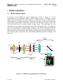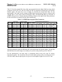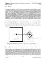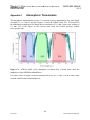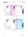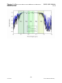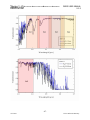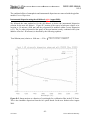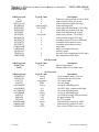
1
OSIRIS
OH- Suppressing Infra-Red Imaging Spectrograph
“Not Your Grandma’s Spectrograph”
USERS’ MANUAL
WARNING
Entering Deep Water
If In Doubt, Don’t Go Out
James Larkin, Matthew Barczys, Mike McElwain,
Marshall Perrin, Jason Weiss, Shelley Wright
UCLA Infrared Laboratory
Version 2.3
March 1, 2010
CALIFORNIA ASSOCIATION FOR RESEARCH IN ASTRONOMY
OSIRIS USER MANUAL
V.2.3
Intentionally Blank
-23/15/2010
UCLA Infrared Laboratory
CALIFORNIA ASSOCIATION FOR RESEARCH IN ASTRONOMY
OSIRIS USER MANUAL
V.2.3
A Subset of the OSIRIS team with the dewar on the Keck II Nasmyth Deck.
OSIRIS and CARA members at OSIRIS first light (Keck II remote OPS).
-33/15/2010
UCLA Infrared Laboratory
CALIFORNIA ASSOCIATION FOR RESEARCH IN ASTRONOMY
OSIRIS USER MANUAL
V.2.3
Table of Contents
1
2
OSIRIS Overview ..................................................................................................................... 6
OSIRIS Capabilities.................................................................................................................. 7
2.1 Basic Optical Layout.......................................................................................................... 7
2.2 Lenslet Geometry............................................................................................................... 9
2.3 Filters and Fields of View................................................................................................ 10
2.4 Dispersions and Resolutions ............................................................................................ 16
2.5 Lenslet Fill Factor ............................................................................................................ 19
2.6 Concentricity of the Four Plate Scales............................................................................. 19
2.7 Optical Error Budget........................................................................................................ 20
2.8 Throughputs ..................................................................................................................... 21
2.9 Sensitivities ...................................................................................................................... 22
2.10 Imager ............................................................................................................................ 23
3 Observing with Adaptive Optics............................................................................................. 25
4 Observing procedures ............................................................................................................. 26
4.1 User Interface................................................................................................................... 26
4.2 Field Acquisition.............................................................................................................. 34
4.3 Spectroscopic Calibration ................................................................................................ 36
4.3.1 Telluric Standards ..................................................................................................... 36
4.3.2 Wavelength Calibrations........................................................................................... 36
5 Data Reduction System........................................................................................................... 39
5.1 Major Changes to the Pipeline for Version 2.2................................................................ 41
5.1.1 Changes to the Pipeline for Version 2.1 ....................................................................... 42
5.1.2 Changes to the Pipeline for Version 2.0 ....................................................................... 42
5.2 Installing the Pipeline at Your Home Institution ............................................................. 43
5.3 ODRFGUI: The OSIRIS Data Reduction File GUI ........................................................ 45
5.4 Working Directly with Data Reduction XML Files (DRFs) ........................................... 47
5.5 Reducing a Normal Observation...................................................................................... 49
5.5.2 Output Filename Construction...................................................................................... 51
5.6 Reducing Multiple Darks or Skies into a “Super” File.................................................... 52
5.7 Mosaicking Multiple Science Exposures......................................................................... 53
5.9 Module Descriptions........................................................................................................ 57
5.9.1 Adjust Channel Levels.................................................................................................. 57
5.9.2 Assemble Data Cube..................................................................................................... 57
5.9.3 Calibrate Wavelength.................................................................................................... 58
5.9.4 Clean Cosmic Rays ....................................................................................................... 58
5.9.5 Combine Frames ........................................................................................................... 59
5.9.6 Correct Dispersion ........................................................................................................ 59
5.9.7 Determine Mosaic Positions ......................................................................................... 59
5.9.8 Divide Blackbody ......................................................................................................... 60
5.9.9 Divide by Star Spectrum............................................................................................... 61
5.9.10 Extract Spectra ............................................................................................................ 62
5.9.11 Extract Star.................................................................................................................. 62
5.9.12 Glitch Identification .................................................................................................... 63
5.9.13 Mosaic Frames ............................................................................................................ 64
-43/15/2010
UCLA Infrared Laboratory
CALIFORNIA ASSOCIATION FOR RESEARCH IN ASTRONOMY
OSIRIS USER MANUAL
V.2.3
5.9.14 Remove Crosstalk ....................................................................................................... 65
5.9.15 Remove Hydrogen Lines ............................................................................................ 66
5.9.16 Rename Files............................................................................................................... 66
5.9.17 Save DataSet Information ........................................................................................... 67
5.9.18 Scaled Sky Subtraction ............................................................................................... 67
5.9.19 Subtract Frame ............................................................................................................ 70
Appendix A Detector Performance............................................................................................ 71
A.1 Characterization Data...................................................................................................... 71
A.2 Memory Charge .............................................................................................................. 72
A.3 Fixed Pattern Noise and Artifacts ................................................................................... 73
A.4 Spectrograph Detector and Detector Controller.............................................................. 75
A.5 Optimization of Detector Operating Temperature .......................................................... 77
A.5.1 Temperature Dependence of QE.............................................................................. 77
A.5.2 Temperature Dependence of the Reset Anomaly .................................................... 78
A.5.3 Optimum Operating Temperature............................................................................ 78
A.6 Spectrograph Detector Crosstalk .................................................................................... 78
Appendix B Filter Curves .......................................................................................................... 80
Appendix C Atmospheric Transmission.................................................................................... 84
Appendix D Atmospheric Dispersion........................................................................................ 88
D.1 Instrumental Chromatic Dispersion ................................................................................ 90
Appendix E FITS header keywords........................................................................................... 93
Appendix F History of Instrument Changes / Which matrices to use in reductions................ 102
Appendix G When all else fails … Play Cowboy.................................................................... 105
-53/15/2010
UCLA Infrared Laboratory
CALIFORNIA ASSOCIATION FOR RESEARCH IN ASTRONOMY
OSIRIS USER MANUAL
V.2.3
1 OSIRIS Overview
OSIRIS is an integral field spectrograph (IFS) designed to work with the Keck Adaptive Optics
System. It uses an array of tiny lenses to sample a rectangular patch of the focal plane and
produces spectra at up to 3000 locations simultaneously. There is also an internal diffraction
limited camera with a 20” field of view. Both the camera and spectrograph can operate at
wavelengths between 1 and 2.4 microns. The center of the imaging camera’s field is about 20”
offset from the center of the spectrograph field and both can be used simultaneously with the
same or different filters. The spectrograph has plate scales of 0.020, 0.035, 0.050 and 0.100
arcsec per lenslet. The spectral resolution averages 3800 in the three finest plate scales, but is
closer to 3000 in the 0.100 arcsec plate scale. In the broadband mode each spectrum contains a
full broad band (z, J, H or K) and a total of 16x64 (actually 1019) spectra are taken. In the
narrowband mode, a typical spectrum contains 1/4th of a broad band and an individual exposure
contains between 16x64 to 48x64 spectra depending on the exact filter selected. The imager has
a single fixed plate scale of 0.020 arcsec per pixel and suffers from some vignetting in the
corners of the array. A great deal of thought has gone into trying to make OSIRIS easy to use.
For the spectrograph, the only user selectable items are the plate scale, the filter and the exposure
time. The imager only has a filter and an exposure time setting. A great deal of complexity,
however, is allowed in the observing sequences and the slaving of the imager to the spectrograph.
All setup and control aspects of the instrument are managed by a few GUIs. There is also a data
reduction system that includes a “real-time” reduction of raw frames into cubes for display and
basic analysis. In this real-time mode, it takes about 1 minute for a preliminary data cube to
appear in the “quicklook” display package. The reduction system also includes a growing set of
final reduction steps including correction of telluric absorption and mosaicking of multiple cubes.
That being said, infrared spectroscopy is a fairly complex astrophysical technique, and when
combined with a laser adaptive optics system, and the complexity of over 3000 independent and
overlapping spectra, OSIRIS is not recommended for the faint of heart.
In terms of observing planning, much of the complication actually comes from the AO nature of
the instrument. As an imaging spectrograph, much of the dithering and exposure settings are
quite similar to a traditional infrared camera or spectrograph. Since the infrared background is
bright and complicated, it’s important to obtain sky frames for subtraction, but in some cases
where your object is small, you can build a sky by dithering “on-chip” (in this case “on-lenslet”
but it’s identical). Similarly, telluric standard stars are needed in most cases to remove
atmospheric transmission variations as a function of airmass and wavelength. Like NIRSPEC or
other IR spectrographs, we’ve found that stars near spectral types A0 work well, although others
sometimes use solar analogs. Much of this is discussed in detail within this manual, but we
thought it was important to give you an initial sense of how the instrument works. Basically pick
a filter and platescale then dither on source and on sky. The pipeline will handle much of the rest.
For the latest information on OSIRIS, please always refer to the website
http://www.astro.ucla.edu/~irlab/osiris/ which will have links to the most recent versions of
software and documentation. It also has links to an OSIRIS wiki page for users.
-63/15/2010
UCLA Infrared Laboratory
OSIRIS USER MANUAL
V.2.3
CALIFORNIA ASSOCIATION FOR RESEARCH IN ASTRONOMY
2 OSIRIS Capabilities
2.1
Basic Optical Layout
A schematic of the OSIRIS IFS optical configuration is shown in Figure 2-1. The IF
spectrograph optical configuration consists of three coupled systems: a re-imager, an image
sampler, and a spectrograph. The image sampler is a 2-dimensional array of small lenses or
lenslets located at a re-imaged focal plane of the Keck II AO system. At the focus of each lenslet
a much smaller pupil image is formed that contains all of the light from its portion of the field.
This lenslet array serves to spatially sample the input image. The pupil images are well
separated and serve to define the entrance aperture of the spectrograph section. The dispersion
axis of the spectrographic is rotated slightly compared to the lenslet orientations so that the
dispersed spectra from each spatial location are interleaved across the spectrograph detector.
The spatial scale of the instrument is determined by re-imaging optics in front of the lenslet array.
The re-imaging optics also provides most of the baffling within the instrument including a cold
pupil stop.
Spectrograph
Cold
stop
Lenslet array Adjustable
mask
Collimator optics
(TMA)
Keck II AO
focus
Fixed
grating
Filters
Re-imager collimator
(singlet)
R.I. Camera
(singlet)
Re-imaging optics
Pupil plane
Re-imaged
focal plane
Image sampler
Camera optics
(TMA)
Detector
Figure 2-1: OSIRIS Spectrograph Optical Configuration
-73/15/2010
UCLA Infrared Laboratory
CALIFORNIA ASSOCIATION FOR RESEARCH IN ASTRONOMY
Fold Mirror
& Lenslet Array
OSIRIS USER MANUAL
V.2.3
OSIRIS Optical Layout
Filter
s
Reimaging
Cameras
Grating
AO Focus
Reimaging
Collimators
Spectrograph
Collimator Mirrors (TMA)
Hawaii-2 Detector
Fold
Mirror
Spectrograph
Camera Mirrors (TMA)
Figure 2-2: Rendering of the real optics within the spectrograph leg of the instrument. Note that
the lenslet array is the smallest component. The reimaging optics are fully refractive to reduce
wavefront error, while the spectrograph optics are all off-axis mirrors to eliminate ghosts.
Each lenslet in a given row is the source for a spectrum that is nominally separated by 2 pixels
vertically from the spectrum of the adjacent lenslet in the same row. Each spectrum is also offset
or staggered horizontally. The stagger results from the slight rotation of the lenslet array relative
to the detector. The horizontal stagger should be 32 pixels, but anamorphism introduced by the
TMA in the horizontal direction causes the offset to be reduced to ~29 pixels. This makes better
use of the detector real estate in the horizontal direction by allowing longer spectra to fit onto the
detector.
-83/15/2010
UCLA Infrared Laboratory
CALIFORNIA ASSOCIATION FOR RESEARCH IN ASTRONOMY
OSIRIS USER MANUAL
V.2.3
2.2
Lenslet Geometry
The lenslet array is rotated by 3.6 degrees relative to the dispersion axis of the grating, which
itself is aligned to rows of the detector. This allows the spectra from neighboring lenslets to miss
each other on the detector and to be successfully interleaved. A side-effect of this is that rows
and columns of the lenslet move diagonally across the detector at an angle of 3.6 degrees. To
keep the spectra roughly centered on the array, we stagger the lenslets every 16th row
(tan(3.6)=1/16). So in the end, 51 columns and 66 rows of lenslets are at least partially
illuminated. Figure 2-3 shows the geometry of illuminated lenslets. We refer to the bottom left
lenslet as [1,1]. Note that it is not illuminated.
Broad Band
~16x64
Narrow Band
~48x64
Figure 2-3: 51 columns and 66 rows of lenslets are at least partially illuminated. The pattern above
shows in white the lenslets that are illuminated in the narrow band mode, and in blue for the broad
band mode. Note that in many narrow band filters, not all of the white lenslets are available either
due to order overlap, or that the spectra fall off the detector. See Section 2.3 for exact sizes. Also
note that 15 lenslets marked in red are lost off the top of the detector and are not available.
-93/15/2010
UCLA Infrared Laboratory
CALIFORNIA ASSOCIATION FOR RESEARCH IN ASTRONOMY
OSIRIS USER MANUAL
V.2.3
2.3
Filters and Fields of View
OSIRIS provides four spatial scales to choose from (0.020, 0.035, 0.050 and 100 arcsec per
lenslet). There are also subtle differences in the spatial scales in terms of the effective pupil size
matched to each scale. This leads to differences in terms of the sensitivities and backgrounds of
the four scales. In a little more detail, the scales are achieved by swapping in matched pairs of
lenses that magnify the images onto the lenslet array. As Figure 2-4 shows, they all must have
the same physical length of 700 mm and there are constraints about the physical size and location
of the lens and filter mechanisms. In particular, the magnification is basically the ratio of the
focal length of the camera lens to the collimator lens. For the 20 mas scale, this requires us to go
from an F/15 beam to an F/257 beam or a magnification of 17.1. So its collimator lens has a very
short focal length of only 20 mm, so its cold pupil is roughly 20 mm behind the lens. The
collimator for the coarsest scale is closer to 100 mm, so its pupil is roughly 200 mm from the
input AO focus. In the end, only each of the three fine scales (20, 35 and 50 mas) have a cold
pupil stop mounted with them, while the coarse scale (100 mas) has a fixed cold stop
permanently mounted in the optical path. This has the unfortunate effect that it must be oversized
to allow through all of the other beams and allows through considerable excess thermal
background. In order to lower thermal background at longer wavelengths, in March 2008 the
OSIRIS team smaller pupil sizes designed smaller 100 mas pupils to be used with duplicate K
filters. There are four filter holders and four new pupils that were attached individually for each
duplicate K filter (Kbb, Kn3, Kn4, Kn5). The pupil sizes for each of the scales and the new
effective 9 meter inscribed pupil for the 100mas scale is illustrated in Figure 2-5.
0.020 arcsec scale: This is the only scale that has proper sampling across the AO PSFs for
wavelengths longer than 1.5 microns. So it is optimized for image quality and has a
slightly oversized pupil that is circumscribed around the 10.94 m outer edges of the Keck
telescope. Because of this, it has an elevated thermal background (K=11.2 mag/sq arcsec).
At wavelengths below 2 microns it is primarily read noise limited so the coarser scales
have better raw sensitivity.
0.035 & 0.050 arcsec scales: These two scales are optimized for maximum sensitivity at thermal
wavelengths (K~11.8 mag/sq arcsec). They both have circular pupils equivalent to a 10meter telescope so they slightly clip the edges of the Keck primary. But since they have
coarse sampling, the PSF is not significantly affected.
0.100 arcsec scale: Originally this was only included to help with target acquisition, but many
users have expressed interest in using it for faint targets. There are several important
caveats with using this scale. First, as the scales get coarser, the geometric pupils formed
by the lenslet array grow. Since OSIRIS is a “pupil spectrograph”, the final spectral
resolution and cross contamination between spectra are directly dependent on the size of
the pupils. Diffraction helps to keep the 20, 35 and 50 mas pupils close to the same size
as each other, and the spectral resolution of ~3800 refers to these scales. The 100 mas
scale is coarse enough that even with perfect optics, it would produce a 2x2 pixel blur on
-103/15/2010
UCLA Infrared Laboratory
CALIFORNIA ASSOCIATION FOR RESEARCH IN ASTRONOMY
OSIRIS USER MANUAL
V.2.3
the detector. With aberrations and diffraction this becomes 2.5 to 3 pixels and results in a
reduced spectral resolution of less than 3400, and additional contamination from
neighboring spectra. The pupil is oversized and allows through a great deal of excess
infrared background (K=10.6 mag/sq”). In order to alleviate this excess background at the
coarsest scale, we have installed duplicate K-band filters with their own smaller 100mas
pupils (9-m effective).
Lenslet Location
Camera Lenses
Filter Locations
Cold Pupils
Collimators
AO Focus
Figure 2-4: Optical paths of the four sets of reimaging
optics. In reality, the lenses are mounted
-11in
turrets in wheel mechanisms, but here we show them side by side for comparison.
3/15/2010
UCLA Infrared Laboratory
CALIFORNIA ASSOCIATION FOR RESEARCH IN ASTRONOMY
OSIRIS USER MANUAL
V.2.3
35 & 50 mas pupils
100mas Kband Pupils
10 m
10.94 m
20 mas pupil
100 mas Pupil
Figure 2-5: Scale drawing of the pupils for each of the four plate scales. Note that the 100 mas
pupil is significantly oversized to allow the other scales optical path not to be vignetted. To lower
the thermal background at longer wavelengths there is a smaller 100mas pupil installed just for
the Kband filters (magenta).
-123/15/2010
UCLA Infrared Laboratory
CALIFORNIA ASSOCIATION FOR RESEARCH IN ASTRONOMY
OSIRIS USER MANUAL
V.2.3
There are a total of 23 filters available within the spectrograph. Originally there were 4
broadband filters and 18 narrowband filters, but since installation of the duplicate K-band filters
with smaller 100mas pupils in March 2008, there are now 5 broadband filters and 18 narrowband
filters (we used an “open” position for adding one of the duplicate filters. The combination of
filters and scales results in 88 discreet modes. For each of the broadbands, the spectra fit
completely on the detector in a single exposure for the central 16x64 lenslets. But since the
grating does not move in OSIRIS, the narrow band filters shift on the detector depending on
where they fall within the broadband spectrum. So, for example, the Kn1 spectra from the central
16x64 spectra fall at the short wavelength end of the location where the Kbb spectra fall which is
at the edge of the detector. So lenslets on one side of the central 16x64 are actually more
centered, while those on the other side fall off the detector. This leads to only the central narrow
band filters falling onto the detector for the full 48x64 lenslets. Filters are either extreme (Kn1 or
Kn5 for example) have some spectra off the detector and so have more limited fields of view.
In addition, the Z and J bandpasses are working at 6th and 5th diffraction orders, respectively. So
the neighboring orders fall fairly close on the detector, and order overlap makes the left-most and
right-most lenslets in the narrowbands unusable. Order overlap also limits the wavelength
coverage of the broad band Z filter. The long wavelength half-power point of the Zbb filter lands
in the 7th order on top of 0.999 microns in the 6th order. So typical wavelength extractions are
limited to wavelengths greater than 0.999 microns.
Table 2-1 gives the wavelength range of each filter (50% transmission points are quoted), along
with the # of simultaneous spectra that are obtained in each exposure, the approximate geometry
of the spectra on the sky, and the fields of view for each of the 4 plate scales. In most cases, if a
narrow band filter does not cover 48x64 lenslets, then it is also displaced slightly left or right on
the sky. The planning gui will show the true coverage of each filter compared to the OSPEC
pointing origin. But all filters include the central 16x64 lenslets. Appendix Appendix B gives
the filter transmission curves. Take note that the filters named “Kcb, Kc3, Kc4, and Kc5” in the
OSIRIS planning GUI (OOPGUI) are just duplicate Kbb, Kn3, Kn4, and Kn5 filters with the
smaller 100mas pupil.
-133/15/2010
UCLA Infrared Laboratory
CALIFORNIA ASSOCIATION FOR RESEARCH IN ASTRONOMY
OSIRIS USER MANUAL
V.2.3
Table 2-1: OSIRIS Spectrograph Filters, Scales and Fields of View
Filter
Shortest
Wavelength
Extracted(nm)
Longest
Wavelength
Extracted(nm)
Number of
Spectral
Channels
Zbb
Jbb
Hbb
Kbb*
999*
1180
1473
1965
1176*
1416*
1803
2381
Zn4
Jn1
Jn2
Jn3
Jn4
Hn1
Hn2
Hn3
Hn4
Hn5
Kn1
Kn2
Kn3*
Kn4*
Kn5
1103
1174
1228
1275
1323
1466
1532
1594
1652
1721
1955
2036
2121
2208
2292
1158
1232
1289
1339
1389
1541
1610
1676
1737
1808
2055
2141
2229
2320
2408
Number of
Complete
Spectra
Approx.
Lenslet
Geometry
FOV for
0.020”
FOV for
0.035”
FOV for
0.050”
FOV for
0.100”
1476
1574
1651
1665
1019
1019
1019
1019
16x64
16x64
16x64
16x64
0.32x1.28
0.32x1.28
0.32x1.28
0.32x1.28
0.56x2.24
0.56x2.24
0.56x2.24
0.56x2.24
0.8 x 3.2
0.8 x 3.2
0.8 x 3.2
0.8 x 3.2
1.6 x 6.4
1.6 x 6.4
1.6 x 6.4
1.6 x 6.4
459
388
408
428
441
376
391
411
426
436
401
421
433
449
465
2038
2038
2678
3063
2678
2292
2868
3063
2671
2038
2292
2868
3063
2671
2038
32x64
32x64
42x64
48x64
42x64
36x64
45x64
48x64
42x64
32x64
36x64
45x64
48x64
42x64
32x64
0.64x1.28
0.64x1.28
0.84x1.28
0.96x1.28
0.84x1.28
0.72x1.28
0.90x1.28
0.96x1.28
0.84x1.28
0.64x1.28
0.72x1.28
0.90x1.28
0.96x1.28
0.84x1.28
0.64x1.28
1.12x2.24
1.12x2.24
1.47x2.24
1.68x2.24
1.47x2.24
1.26x2.24
1.58x2.24
1.68x2.24
1.47x2.24
1.12x2.24
1.26x2.24
1.58x2.24
1.68x2.24
1.47x2.24
1.12x2.24
1.6 x 3.2
1.6 x 3.2
2.1 x 3.2
2.4 x 3.2
2.1 x 3.2
1.8 x 3.2
2.25x3.2
2.4 x 3.2
2.1 x 3.2
1.6 x 3.2
1.8 x 3.2
2.25x3.2
2.4 x 3.2
2.1 x 3.2
1.6 x 3.2
3.2 x 6.4
3.2 x 6.4
4.2 x 6.4
4.8 x 6.4
4.2 x 6.4
3.6 x 6.4
4.5 x 6.4
4.8 x 6.4
4.2 x 6.4
3.2 x 6.4
3.6 x 6.4
4.5 x 6.4
4.8 x 6.4
4.2 x 6.4
3.2 x 6.4
*
Limited by overlap from other orders.
* The Kcb, Kc3, Kc4, and Kc5 filter names are identical to these respective filters.
-143/15/2010
UCLA Infrared Laboratory
CALIFORNIA ASSOCIATION FOR RESEARCH IN ASTRONOMY
OSIRIS USER MANUAL
V.2.3
Table 2-2 lists the original filter lists of the spectrograph before the March 2008 servicing which
swamped out the Zn2, Zn3, and Zn5 filters for the new duplicate K-band filters with smaller
100mas pupils. The first four rows of Table 2-2 describe the broad band filters for the
spectrograph. The table lists the original OSIRIS filter specifications (first two columns titled
“Design Specs”), the actual central wavelength (CWL) and bandwidth (BW) as measured in
OSIRIS in the next two columns, and the remaining columns to the right list the filter parameters
for the actual filters as measured by the filter manufacturer.
Table 2-2: OSIRIS Spectrograph Filter Parameters
Design Specs
Filter Name
CWL (nm)
BW (nm)
Measured in OSIRIS
CWL (nm)
BW (nm)
CWL (nm)
BW (nm)
Test Data Supplied by Filter Manufacturer
Avg T
Rise
Fall Slope RMS wfe
(%)
Slope (%)
(%)
(waves)
83.8
1.76
2.15
0.021
P-V wfe
(waves)
0.095
Not avail.
Power
(waves)
0.044
Zbb
1090.0
220.0
1090
220
1089.5
218.8
Jbb
1310.0
260.0
1325
303
1309.7
260.1
78.9
2.04
1.20
Hbb
1636.0
330.0
1637
347
1637.9
329.5
92.6
1.17
1.21
Kbb
2180.0
440.0
2174
423
2172.8
415.7
85.5
1.08
1.30
0.014
0.081
-0.003
Zn2
1046.0
54.4
1046
55
1044.5
51.3
69.8
0.75
0.62
0.019
0.095
0.041
Zn3
1089.0
54.7
1089
54
1086.7
52.6
71.6
0.82
0.58
0.021
0.121
0.049
Zn4
1132.0
55.1
1132
57
1130.5
54.6
77.6
0.62
0.81
0.014
0.099
0.012
Zn5
1177.0
56.4
1176
58
1176.2
56.3
72.8
0.62
0.77
0.010
0.074
0.002
Jn1
1204.0
64.6
1203
51
1202.8
58.4
77.8
0.64
0.59
0.024
0.125
0.047
Jn2
1256.0
65.0
1260
66
1258.3
60.8
78.0
0.65
0.73
0.018
0.105
0.021
Jn3
1308.0
65.5
1309
68
1306.9
64.5
84.2
0.72
0.63
0.017
0.085
0.049
Jn4
1359.0
65.9
1358
70
1356.3
65.8
82.3
0.65
0.63
0.020
0.090
0.050
Hn1
1505.0
81.0
1500
77
1503.3
74.7
80.9
0.68
0.71
0.009
0.055
0.027
Hn2
1570.0
81.6
1569
86
1570.8
77.6
75.2
0.72
0.76
0.016
0.087
0.040
Hn3
1635.0
82.1
1635
88
1634.8
81.4
79.5
0.66
0.71
0.012
0.064
0.034
Hn4
1698.0
82.6
1695
92
1694.1
84.9
83.3
0.68
0.76
0.018
0.083
0.056
Hn5
1765.0
85.1
1766
94
1764.4
86.1
74.8
0.66
0.97
0.013
0.093
-0.021
Kn1
2006.0
108.0
2011
94
2004.8
100.1
85.1
0.74
0.70
0.004
0.067
-0.002
Kn2
2093.0
108.7
2091
110
2088.4
104.5
83.4
0.94
0.77
0.004
0.025
-0.007
Kn3
2179.0
109.4
2177
114
2175.4
108.0
83.8
0.72
0.90
0.017
0.070
-0.054
Kn4
2265.0
110.1
2264
118
2263.8
112.6
75.0
0.80
0.72
0.019
0.109
-0.020
Kn5
2353.0
112.8
2348
120
2349.9
116.5
79.5
0.78
0.72
0.013
0.088
0.039
Not avail.
All of the measured values for BW and CWL are based on the 50% power points. For the Zbb
and Jbb filters, the useful ranges are actually set by order overlap and are given in Table 2-1.
For the manufacturer’s test data slope, is determined based on the 80% and 5% relative
transmission points. The wavefront error (wfe in the table), peak to valley wavefront error (P-V
wfe in the table) and the optical power are given in wavelengths of light (waves) at 632.8 nm.
-153/15/2010
UCLA Infrared Laboratory
CALIFORNIA ASSOCIATION FOR RESEARCH IN ASTRONOMY
2.4
OSIRIS USER MANUAL
V.2.3
Dispersions and Resolutions
OSIRIS can take up to 3072 spectra simultaneously. Due to variations in the incident and
diffracted angles with the grating, and with spot quality at the detector, the spectral resolution
has significant variation between lenslets and at different wavelengths. The dispersions on the
detector are actually fairly constant and have median values given in Table 2-3.
Table 2-3: Linear Dispersion
Band (order)
Z (6th)
J (5th)
H (4th)
K (3rd)
Median Dispersion
per pixel in raw data
(μm/pix)
0.0001410
0.0001692
0.0002115
0.0002820
Resampled Dispersion
in Reduced Cubes
(μm/pix)
0.000120
0.000150
0.000200
0.000250
Over the central 16x64 lenslets which include the full broad band, the median spectral resolution
in the 0.050” scale is 3900, and the average resolution is 3600. The difference comes from the
fact that the long wavelength end of spectra tend to have fairly constant resolutions just above
4000, while the short wavelengths within each order fall to about 2800. Figure 2-6 shows the
spectral resolution achieved at a wavelength of 2.190 microns. Notice the bright region near
lenslet [38,12] where the FWHM is typically less than 2 pixels leading to a spectral resolution
above 4500. Towards the lower right, the FWHM begins to increase and the spectral resolution
bottoms out around 2800. The graph in Figure 2-7 shows the more complex variation of spectral
resolution as a function of position and wavelength.
-163/15/2010
UCLA Infrared Laboratory
CALIFORNIA ASSOCIATION FOR RESEARCH IN ASTRONOMY
OSIRIS USER MANUAL
V.2.3
Figure 2-6: This is the effective spectral resolution achieved as a function of lenslet position at a
wavelength of 2.190 microns. It includes the linear dispersion and the measured FWHM of an
arcline at this wavelength. Notice that spectral resolutions are highest near lenslet [38, 12] and
are lowest near lenslet [22,50]. For numeric values, use the graph shown in Figure 2-7.
-173/15/2010
UCLA Infrared Laboratory
CALIFORNIA ASSOCIATION FOR RESEARCH IN ASTRONOMY
OSIRIS USER MANUAL
V.2.3
Best Lenslet
Median Lenslet
Worst Lenslet
Figure 2-7: The spectral resolution depends on lenslet number and wavelength. This graph
shows the resolution as a function of wavelength in the 3rd order (K band) over the primary
16x64 lenslet positions (median resolution at each wavelength), the highest resolution region
(lenslets near [22, 50]) and the lowest wavelength region (lenslets near [38,12]). Other bands
are simple scalings of this relationship, i.e. the J band is observed in 5th order, so the same
resolution occurs at 3/5ths of the wavelengths shown in the graph. This is for the 0.050” scale,
although the 0.020” and 0.035” scales are similar.
-183/15/2010
UCLA Infrared Laboratory
CALIFORNIA ASSOCIATION FOR RESEARCH IN ASTRONOMY
2.5
OSIRIS USER MANUAL
V.2.3
Lenslet Fill Factor
According the test report supplied by the manufacturer there is a 2-3 micron rounding between
the nominally square lenslets. This results in a fill factor of approximately 95%.
Additionally, the test report supplied by the manufacturer indicates that the transmittance of the
lenslet array is between 95 % and 97%. The peak transmittance is at 1.2 µm.
2.6
Concentricity of the Four Plate Scales
An important consideration is how well aligned are the four spectrograph plate scales. If you
acquire an object in the center of one scale, then you can NOT simply select another scale and
remain centered on your object. Table 2-4 below gives the relative offset between the field
centers of the four scales. It is important, however, to remember that if an object appears
centered in the 0.100” scale, this represents 5 pixels within the 0.020” scale, so a small shift in
addition to the table offsets may occur. The table assumes that an object has been centered in the
0.020” scale and then calculates by how much it will shift in reduced data cubes if another scale
is selected and the object is not moved. X-offset refers to the short (16 or 48 lenslet) axis, while
the Y-offset refers to the long (64 lenslet) axis.
Table 2-4: Relative Offsets between the Four plate Scales.
Scale
0.020”
0.035”
0.050”
0.100”
Xoffset (arcsec)
≡0.000
-0.02
-0.04
0.01
Yoffset (arcsec)
≡0.000
0.08
0.10
0.00
To compensate for these small offsets, the Telescope GUI (OTGUI) can be used to offset an
object from the center (or specified pixel) in one plate scale to the center (or specified pixel) in
another plate scale, or even to the imager.
-193/15/2010
UCLA Infrared Laboratory
CALIFORNIA ASSOCIATION FOR RESEARCH IN ASTRONOMY
2.7
OSIRIS USER MANUAL
V.2.3
Optical Error Budget
In Table 2-5 below, we give the estimated RMS wavefront error of each optical element in the
spectrograph up to but not including the lenslet array and all elements of the imager. These are
the elements that affect the Strehl ratios. In the case of mirrors, the wavefront error is assumed
to be twice the surface error. For the window, lenses and filters the wavefront error is assumed
to be equal to (n-1) times the sum in quadrature of the two surface errors. In all cases, the
measurements were made over an area equal to or larger than the illuminated region. In some
cases, more than one component was fabricated, and the component currently in the instrument is
identified in the table.
Table 2-5:Optical Error Budget
Component
Window (1) (n=1.458)
Window (2)
Window (3)
Splitter Mirror Spectrograph (1)
Splitter Mirror Spectrograph (2)
Splitter Mirror Imager (1)
Splitter Mirror Imager (2)
Lenslet Fold Mirror (1)
Lenslet Fold Mirror (2)
Spectrograph Fold Mirror (1)
Spectrograph Fold Mirror (3)
Spectrograph Fold Mirror (4)
Imager Fold Mirror (1)
Imager Fold Mirror (2)
F/257 Collimator (n=1.474)
F/257 Camera (n=1.474)
Imager M1
Imager M2
Imager M3
Imager M4
Filters (min:mean:max)
Imager Surface Total (alignment
errors ignored)
Imager design WFE
Imager alignment tolerances
Design RMS WFE (nm)
4
4
4
13
13
13
13
13
13
13
13
13
13
13
17
17
21
21
21
21
12
50
Fabricated RMS WFE (nm)
3
3.8 (will be installed at summit)
4.4 (in dewar)
3 (in dewar)
13
8 (in dewar)
9
12
14 (in dewar)
6 (in dewar)
8
4
8
3 (in dewar)
14
9
6
10
6
16
2:5.5:10
23
25
30
Spectrograph Total (0.02 scale)
Imager Total (design+align+surface)
35
24
<45
The 0.020” scale is very insensitive to alignment issues, since there are only two powered optics
and these are simple biconvex lenses. Tipping or tilting them to first order causes image motion.
Sufficient tilt to contribute to the wavefront error budget would shift the images off the small
lenslet field. The same is true of the coarser scales, but they are also much more tolerant to
wavefront error due to sampling issues. So the spectrograph tip/tilt and decenter requirements
-203/15/2010
UCLA Infrared Laboratory
OSIRIS USER MANUAL
V.2.3
CALIFORNIA ASSOCIATION FOR RESEARCH IN ASTRONOMY
from the OSIRIS Mechanical Design Note (OMDN) 01.00 Section 5 must be satisfied in order to
achieve the observed image quality.
The imager has three powered surfaces, but these are also spherical which are relatively
insensitive to alignment errors. To reach the 30 nm of WFE allowed for imager internal
alignment, the detector would be focused 7 mm from nominal which would be easily seen in our
mounting, and would shift the plate scale away from our measured value of 0.020” by more than
5% which is not observed in either measurement method. This level of alignment error also tends
to make the plate scales in each direction different which is not observed.
2.8
Throughputs
In this section we summarize the vendor data on individual component efficiency, along with the
estimate of the grating efficiency as derived from the relative efficiency of the spectrograph and
imager. For simple elements such as the gold mirror or BaF2 lenses, we use the coating
reflectances or transmittances supplied by the coating vendor. Notice that the measured
efficiencies in the H and K bands are comparable to each other but about 30% lower than
expected. We have somewhat arbitrarily assigned the majority of this to the grating. In the Jband, however, the efficiency falls dramatically to only 2.7%. We do not know the source of this
efficiency loss, and we believe it is unfair to assign the full extent to OSIRIS. We note that
NIRC2 appears to have at least a factor of 2 loss of efficiency from the K to the J bands.
Table 2-6 lists the component efficiencies as presented at the PDR and as-built.
Table 2-6: Predicted and As-built Efficiencies
OPTICAL ELEMENT
Window
Fold Mirrors
Collimator Lens
Filters
Camera Lens
Lenslet Array (AR Coated, 2 surfaces)
TMA Collimator (4 mirrors, 99%; includes first
fold)
Grating (varies with wavelength)
Camera Optics (4 mirrors, 99%; includes fold)
Efficiency predicted
at PDR
97%
NA
92%
75%
92%
96%
96%
70% peak
96%
Total Optical Throughput
Detector Quantum Efficiency
OSIRIS Total Throughput
38%
65%
25%
Telescope Transmission
AO Transmission
Atmosphere
80%
65%
90%
TOTAL THROUGHPUT
12%
As-built measured efficiency
(H and K bands)
97%
96%
96%
70-93% (avg. = 80.0%)
96%
95%
92% (assumes some dirt)
42% avg
92%
23%
81%
19%
80%
65%
90%
8.8%
-213/15/2010
UCLA Infrared Laboratory
CALIFORNIA ASSOCIATION FOR RESEARCH IN ASTRONOMY
2.9
OSIRIS USER MANUAL
V.2.3
Sensitivities
OSIRIS object sensitivities are a little more complicated to calculate than with a normal
instrument. The OSIRIS throughput varies through each band due to the atmospheric
transmission, blaze function of the grating and filter functions. With an imager all of these
factors can often be combined into a single zero point for each filter. But for a spectrograph,
there is in essence a different zero point for every spectral channel. In addition, the 3000+ spectra
all have slight variations in efficiency primarily due to detector effects, and different angles and
footprints on the grating. There is also the added complexity of adaptive optics imaging and the
unpredictable Strehl ratio that you will achieve on your science target. Nevertheless, OSIRIS
offers substantially better capability for true spectral photometry compared to a traditional slit
spectrograph due to its integral field nature. So in principle the PSF can be fully characterized,
and in most cases point sources are fully covered by the fields of view. For sensitivity
calculations each spectrum is spread over more than one detector pixel, so the extraction
algorithm “sweeps” up more than one pixel’s worth of noise. The amount of read noise per
spectral channel therefore depends weakly on plate scale and wavelength. The best demonstrated
read noise per pixel using the up-the-ramp sampling method is 4.8 electrons (this actually also
includes a dark current and detector glow component). With the new grating installed in June,
2005, arclines are more elongated perpendicular to the dispersion axis than at the time of preship.
This leads to more read noise per spectral channel than with the original grating, although several
other factors including throughput improved dramatically. A typical read noise component for
extracted spectra is about 10 electrons in the up-the-ramp mode.
In Table 2-7 below, we give the zero points for the OSIRIS spectrograph expressed in extracted
DN/sec. In these units, the zero points are defined in the standard way:
Mag = -2.5 log(flux in DN/sec) + Mag(zero point)
Table 2-7: Spectrograph Zero Points
Spectrograph Zero Points
(if flux is in DN/sec)
23.5 mag
24.3 mag
23.7 mag
Band
J
H
K
To convert to electrons, assume a detector gain of 0.23 DN per electron. To calculate rough
sensitivities for a continuum source, estimate the flux per lenslet element for your target
assuming a reasonable Strehl ratio (see the AO page for expected Strehls with the Laser or NGS
targets). You can then use the zero points to determine the number of data numbers per lenslet
that will be generated per second. Multiply this by your exposure time, and divide by 1700
(roughly the number of spectral channels). This will give you the number of DN per spectral
channel, and compare that to 4 data numbers to get a rough signal to noise for an individual
exposure for each lenslet.
-223/15/2010
UCLA Infrared Laboratory
CALIFORNIA ASSOCIATION FOR RESEARCH IN ASTRONOMY
2.10
OSIRIS USER MANUAL
V.2.3
Imager
The imager uses a Hawaii-1 detector from Rockwell Scientific and has a 1024x1024 pixel format.
The plate scale is 0.020 arcsec per pixel for a total field of view of 20.4 arcsec. It is sensitive
from 1 to 2.5 microns. The minimum exposure time is 2 seconds and times are limited to integer
seconds. The imager holds virtually an identical set of filters as the spectrograph, but due to
space within the filter wheels, does not have Zn2, Zn4, Zn5 or Jn4 filters (see Table 1). The
imager field is offset from the spectrograph so that both can be used simultaneously without the
need for beam splitters or dichroics. There were several motivations for the imager, including
field acquisition and imaging science. But the primary purpose of the imager, and the reason for
simultaneous viewing, is to track changes in the point spread function (PSF). As with all
adaptive optics systems, the image quality is continuously changing and is difficult to predict
purely from the wavefront sensor data. Also, for many science cases, the spectrograph target
cannot be used to measure its own PSF. So the imager’s goal is to measure the PSF from off-axis
stars to at least allow for monitoring of the variation of conditions with time. Making use of the
PSF stars to predict the PSF at the science target is still a major goal of many adaptive optics
groups and is not a fully solved problem. The imager and spectrograph are in a fixed orientation
compared to each other, but they can be dithered on the sky, and the pattern can be rotated to
arbitrary angles.
19.4”
Spectrograph Fields:
Up to 4.8”x6.4” at approximately
45 degrees
Imager Field
20.4”x20.4”
Horizontal plane of Keck II AO bench and OSIRIS internal optical bench
Figure 2-7: Relative locations of the imager and spectrograph focal planes.
For the imager, in most cases you will be background limited. So the noise is dominated by the
sky background. As you can see, the background in the K band is significantly elevated over
NIRC or NIRSPEC. This is primarily due to the increased background from the AO system, but
it is also due to the optical design of the imager. It is based on the SHARC camera and is close to
an Offner optical design. This leads to excellent image quality with simple optics, but the pupil is
poorly formed and not directly on an available optical surface. So the cold pupil is oversized and
allows through additional background. Due to this background, the H band is definitely the
deepest imaging filter. But care must be taken for some sources, since all of the OSIRIS filters
-233/15/2010
UCLA Infrared Laboratory
CALIFORNIA ASSOCIATION FOR RESEARCH IN ASTRONOMY
OSIRIS USER MANUAL
V.2.3
were designed around the blaze functions of the OSIRIS spectrometer. These filters are typically
wider than traditional infrared filters and photometric corrections will be necessary for objects
with extreme colors, or that are line dominated. Filter curves are given in Appendix C.
Band
J
H
K
Imager Zero Point and Background
Zero Point
Background
mag (in DN/sec)
mag / sq arcsec.
27.8 mag
16.2
28.1 mag
14.6
27.6 mag
10.6
-243/15/2010
UCLA Infrared Laboratory
CALIFORNIA ASSOCIATION FOR RESEARCH IN ASTRONOMY
OSIRIS USER MANUAL
V.2.3
3 Observing with Adaptive Optics
Coordination between OSIRIS and the AO system is largely handled automatically, but the user
needs to be aware of certain limitations. Pre-observing planning on each science target is needed.
The relative position of the guide star to the science fields is not completely arbitrary due to the
position of the AO system’s optical axis with respect to the OSIRIS optical axis, and the range of
travel of the AO Field Steering Mirrors. A planning tool to help determine the ranges of position
angles that are possible for a given guide star/science object geometry is available at
http://www2.keck.hawaii.edu/software/findChartGW/acqTool.php.
-253/15/2010
UCLA Infrared Laboratory
CALIFORNIA ASSOCIATION FOR RESEARCH IN ASTRONOMY
OSIRIS USER MANUAL
V.2.3
4 Observing procedures
4.1
User Interface
Observational Planning GUI
The OSIRIS planning GUI (OOPGUI) is your main interface for making observations. It allows
users to plan observational sequences on one field with both the spectrograph and imager.
Observers are able to change the filter, scale, coadds, itime, and dither patterns. The “Dataset”
and “Object” fields are used for header information. The “LGS mode” is used to determine
whether the laser should be dithered with your dither pattern or if it should remain fixed on-axis.
IMPORTANT: The Kcb, Kc3,
Kc4, and Kc5 filters are
designed to only be used with
100 mas scale. Users must select
both the combination of “Kc”
filter and the 100mas scale!
-263/15/2010
UCLA Infrared Laboratory
CALIFORNIA ASSOCIATION FOR RESEARCH IN ASTRONOMY
OSIRIS USER MANUAL
V.2.3
In practice, we’ve found that the fixed position is optimal. The dither pattern is determined
within the “Object Frames” and “Sky Frames” fields. For instance, in the above example the
observer has set up three exposures on the science target (frames 1,2,3) with a raster scan and
two additional sky frames. The first sky frame (frame 4) is offset from the science target by 5”
west and 5” north, and the second sky frame (frame 5) is offset relative to the first sky frame by
0.35” west. There are multiple dither pattern options to select from: Stare (no dither), Box 4, Box
5, Box 9, Raster Scan, Statistical, and User Defined. The “Show Position List” button opens
another window (bottom left image) that lists all the frames with their x and y offsets of the
dither positions. It shows sky frames and the sequence of the observations. You may change the
order of the frames by selecting one of the frames and using the Up, Down, Top, and Bottom
buttons, as demonstrated on the bottom right image, which now has the last sky frame (number
5) being taken at the beginning of the observation sequence.
-273/15/2010
UCLA Infrared Laboratory
CALIFORNIA ASSOCIATION FOR RESEARCH IN ASTRONOMY
OSIRIS USER MANUAL
V.2.3
If you are taking imager frames as well, the dither pattern chosen will reflect both the
spectrograph and the imager since they are fixed relative to each other (bottom left image). The
imager has several options: Disable (SPEC only), Independent (Imager only), Maximum Repeats,
Maximum Itime, and Filter Sets. The Maximum Repeats, Maximum Itime, and Filter Sets are all
based on the total integration time of the SPEC frames. The Maximum Repeats does the
maximum number of imager frames with a user specified imager itime. The Maximum Itime
calculates the maximum itime the imager can do given a user specified number of repeats. The
Filter Sets is the most flexible option and allows users to use more than one filter and to directly
specify the itime, coadds, number of repeats for each filter. When you select the “Filter Sets”
option and click on the Filter field another window opens (bottom right image) for the user to
interact with each of the values.
Altering any of these fields in the GUI does not directly communicate with the instrument
or the telescope. Once the observation sequence is prepared click the “Send to Queue” button,
which adds the Dataset script (called a Data Definition File or .DDF) to a directory queue which
the execution client GUI uses to build a list of observations. It’s important to note that the
position angle (PA) input does not alter the PA of the instrument once the DDF is executed.
Altering the PA needs to be performed in the Telescope GUI (OTGUI). The correct PA is
critical to make the proper dithers when moving in “sky” coordinates. Users may also save
their observation planning sequence (.DDF) for later use or for planning before they arrive at the
telescope. The GUI can be downloaded to your home computer before your run so you can
practice laying out your observations. It’s available at the OSIRIS website:
http://www.astro.ucla.edu/~irlab/osiris/
-283/15/2010
UCLA Infrared Laboratory
CALIFORNIA ASSOCIATION FOR RESEARCH IN ASTRONOMY
OSIRIS USER MANUAL
V.2.3
Execution Client GUI
The execution client is the GUI that manages your observing sequences and implements them
with the hardware control software. Once you have planned your observations in the OOPGUI
(described above) you will “Send to QUEUE”, which sends your planned observations to this
GUI. Once you are ready to start your observations you
click “Start Next Dataset” which then commands the
instrument and telescope. You only run this GUI at the
telescope and it’s easiest to learn at the telescope. It
only has a few options including removing sequences
that you don’t want to execute, and starting sequences
in the queue. For convenience, it also has the ability of
starting spectrometer or imager frames using the current
exposure settings.
If you decide during an observational sequence that you
wish to terminate or stop the sequence CAUTION
should be taken. In most cases users should always use
the “Abort After Current Spec”, which allows the
current integration to finish exposing (with no effects to
the detector) and then terminates the rest of the
observing sequence. The “Abort All Immediately”
should be used ONLY in dire need. This will stop the
observation sequence in mid integration and resets all
the voltages of the detector controller, which causes
detector thermal problems which may take up to 15
minutes to clear. Flushing the detector will become
necessary before resuming observations. Please see the
Telescope GUI (OTGUI) section for instructions on
how to flush the detector.
-293/15/2010
UCLA Infrared Laboratory
CALIFORNIA ASSOCIATION FOR RESEARCH IN ASTRONOMY
OSIRIS USER MANUAL
V.2.3
Status GUI
The Status GUI presents the current positions of all the motor mechanisms of OSIRIS
spectrograph and imager. When the mechanisms are physically moving in the instrument the
wheeled images will move on the GUI. The integration of a current file in the spectrograph and
imager are updated as the exposure is being taken for monitoring.
-303/15/2010
UCLA Infrared Laboratory
CALIFORNIA ASSOCIATION FOR RESEARCH IN ASTRONOMY
OSIRIS USER MANUAL
V.2.3
Telescope GUI
The OSIRIS telescope GUI is used to input and send all commands to the telescope. The white
box is used for logging which commands where issued. The GUI has a set of tabbed headings
which bring down different control options.
• The Cover folder is blank and hides the other folders so observers do not
accidentally click and move the telescope. The GUI will automatically switch to
this cover when not in use.
• The Offset folder allows users to center the spectrograph between different modes
(filter and scale), and offset to the imager. It also allows users to offset in RA and
DEC in arcsec or detector pixels (it will use the current scale of the instrument so
check the status GUI).
• The Rotate folder changes the position angle of OSIRIS.
• The Adaptive Optics folder allows input “wait4ao” ON or OFF. The script
"wait4ao” determines whether you want the observations to wait for the AO loops
(DM and TT) to close before taking an exposure. You can either select wait4ao
which includes both the DM and TT or wait4dm or wait4tt ON or OFF,
• The OSIRIS folder allows you to flush the spectrograph and imager detector. It
takes a number of short integrations to clear the detector. This should only be
done if persistence is seen in the detector from a bright star or if there are detector
artifacts after issuing the command, “Abort All Immediately”.
-313/15/2010
UCLA Infrared Laboratory
CALIFORNIA ASSOCIATION FOR RESEARCH IN ASTRONOMY
OSIRIS USER MANUAL
V.2.3
On-line Reduction GUI
At the telescope, the OSIRIS pipeline is always waiting for a new raw file to be written so the
little oompa loompas can generate a reduced cube for observational viewing and acquisition
needs. The on-line reduction GUI (OORGUI) allows observers to select the calibration files for
the Subtract Frame and Extract Spectra modules. In most cases, there should be no need to edit
the calibration file for the Extract Spectra module since the GUI will automatically select the
most recent rectification matrix based on the observed filter and scale. The Subtract Frame
module can either use a specified FITS file, the first file generated from a dataset, or the second
file generated from a dataset. For example, if dataset number 32 had two frames where frame 1
was a star and frame 2 was sky, then you would select “Next Raw Frame”. If instead dataset
number 32 had two frames where frame 1 was sky and frame 2 was the star, then you would
select “Previous Raw Frame”. If the Skip module is selected for a blue highlighted module, then
that module will not be used in the pipeline and will be greyed out (i.e., Remove Crosstalk
module in the image below) in the GUI. Please refer to Section 5 for a detailed description of the
Data Reduction Pipeline.
-323/15/2010
UCLA Infrared Laboratory
CALIFORNIA ASSOCIATION FOR RESEARCH IN ASTRONOMY
OSIRIS USER MANUAL
V.2.3
Quicklook2
OSIRIS spectrograph frames are 3D FITS files that require sophisticated image visualization
tools. The OSIRIS team presents an IDL based software package called Quicklook2 to display
and analyze your OSIRIS data cubes. Quicklook2 is the OSIRIS image analysis software used at
Keck while observing, but we also encouraged using Quicklook2 for post-observing analysis of
2D/3D FITS. This software handles simple image analysis functions such as horizontal and
vertical cut plotting, surface and contour plotting, color stretching, photometry analysis, image
arithmetic, and zooms. At the same time, Quicklook2 is equipped with enhanced image analysis
procedures for image rotations, wavelength information, and line fitting. The main image
analysis GUI in Quicklook2 is shown below for reference. For a complete description of
Quicklook2 functionality and operating procedures, please see the Quicklook2 Users’ Manual,
which is available for download at the url http://www.astro.ucla.edu/~irlab/osiris/. This manual
also has detailed instructions on installing Quicklook2 onto local machines. This software
package supports the UNIX, Linux, Mac OS, and Windows operating systems.
-333/15/2010
UCLA Infrared Laboratory
CALIFORNIA ASSOCIATION FOR RESEARCH IN ASTRONOMY
OSIRIS USER MANUAL
V.2.3
Field Acquisition
4.2
As an imaging spectrograph, it is easier to acquire targets with OSIRIS than with traditional slit
spectrometers, but the AO system and some details of the instrument can make field acquisition
non-trivial. Most observations require a separate tip/tilt (TT) star for AO correction. Since
acquisition of science targets is often performed as a blind offset from this star, it is imperative
that the coordinates of the science target and the TT star are consistent with each other. Given
the small field of view of the OSIRIS spectrograph, small errors in position can leave the science
target just off the field. Given the faint nature of many science targets, it is easy to waste time
integrating at the region adjacent to your science target. Please pay attention to issues such as
mismatches in coordinates between catalogs, which can be particularly prevalent between older
and newer stellar catalogs, such as HD and HST. Also, proper motions of stars can be significant
between your observing date and the observing epoch in a catalog. Remember that for OSIRIS
being off by just 1 arcsec can make a big difference!
In general, it is very important to use the Keck’s AO planning tools before your run to determine
the position angles and offsets from your tip-tilt stars. For large offsets from the star, you may
need to use different PAs so that both spectrograph and imager frames can be taken without
defaulting the AO field steering mirrors (FSM). However, if your science is purely with the
spectrograph, then in most cases you do NOT need to take acquisition frames with the imager
first.
The procedure below is the most common type of acquisition: acquiring a science target directly
to the spectrograph. Important to the acquisition process is putting targets accurately at the
center of the spectrograph field of view, which is called the OSPEC pointing origin by the
telescope software. The OSPEC pointing origin is the center of reduced cubes in the 0.020”
scale for all broadband filters and the narrowband filters Zn3, Jn3, Hn3 and Kn3. For the other
plate scales and filters, the center of the field is slightly offset (see Section 2.6 and the OTGUI of
Section 4.1). During the afternoon, your support astronomer will typically use the fiber source in
the AO system to refine this pointing reference.
The acquisition procedure to place a science target on OSPEC is as follows:
(1) Ask the OA to slew the telescope to the primary TT star of your desired science target
(2)
During the slew, adjust the position angle to the desired value using Rotate tab on the
OTGUI (See Section 4.1).
(3)
When the rotation is complete, locate the TT star on the guider display using a finding
chart. Ask the OA to acquire the TT reference star to the OSPEC pointing origin by
giving the pixel coordinates of the TT star on the guider (often this will be obvious
and the OA will immediate acquire the star). The OA should acquire to the OSPEC
pointing origin using the “Adjust Pointing” button on xguide. The TT star should
now be centered on OSPEC.
-343/15/2010
UCLA Infrared Laboratory
CALIFORNIA ASSOCIATION FOR RESEARCH IN ASTRONOMY
OSIRIS USER MANUAL
V.2.3
(4)
If you are planning to take science frames in the 0.020” scale in a filter for which
OSPEC is the center (see above), skip to the next step. Otherwise, you must
perform an offset to put the TT star in the center of your working scale and filter.
On the Offset tab of the OTGUI, perform a move from the “center” of any OSPECcentered filter in 0.020” mode to the “center” of the scale and filter you plan to use
for your science.
(5)
Once you’ve moved the star to your particular center location, take an on-source and
off-source (or sky) pair of images. Using the OOPGUI, define a dataset with a
“stare” exposure with no offset as the object frame, and a “stare” exposure with an
offset of ~5 arcsec as the sky frame. When the second exposure is complete, the
online DRP will produce a data cube containing the star. The online DRP reduction
should take about a minute.
If the star is in the field but does not appear in the center, use the OTGUI to move it
to the center position by specifying which pixel the star is currently located on and
move it to the field center. Make sure the filter and scale are both set to your
working scale and wavelength.
If the star does not appear in the field at all, make sure that the AO system is still
locked on the star, and that you are at the OSPEC pointing origin (ask your OA). If
everything seems right but you don’t see the star, it may be off the field. Try
switching to a narrow band filter in the 0.100” scale to get the maximum field of
view (4.8”x6.4”). If the star is faint, try increasing the exposure time (although 60
seconds should be sufficient to see any TT star).
If desired, you can take a pair of exposures to verify the centering of the TT star.
However, this is not normally needed, and it will cost you time for the exposures
and reduction. This is normally not necessary, but one option would be to start the
exposures and go on to the next step while you wait for the pipeline to finish.
(6)
Once the TT star is centered, ask the OA to “Mark Base” (this is particularly important
for the Mosaic Frames module, see Section 5.7). This will set the current offset
values to zero and make the telescope RA and DEC keywords match the sky. Then,
ask the OA to “Offset to science target”, which will place your science target on the
OSPEC pointing origin. In LGS-AO operations, the OA will acquire using LGSAO-Acq on OSPEC.
(7)
Begin science observations.
-353/15/2010
UCLA Infrared Laboratory
CALIFORNIA ASSOCIATION FOR RESEARCH IN ASTRONOMY
4.3
OSIRIS USER MANUAL
V.2.3
Spectroscopic Calibration
4.3.1
Telluric Standards
The atmosphere in the infrared has significant transmission variation both with wavelength and
with time. In order to properly reduce a spectrum, this transmission must be estimated at an
elevation and atmospheric condition close to your science target. We recommend using an A0
star within 0.1 airmasses of your science exposure. Stars with magnitudes between 7 and 9 work
well and typical exposure times are 20 seconds. If you spend roughly an hour on a given target
field, we often select a telluric star at about the same declination but 30 minutes later in RA from
the science target. This will place the star at about the average location in the sky that the science
exposures were taken.
The pipeline modules Extract Star, Remove Hydrogen Lines and Divide by Blackbody work to
produce a 1D spectrum of a star taken for telluric correction. To work properly, the star must be
at least 4 pixels from the field edges and must have no significant spectral features besides
hydrogen absorption lines. This typically means using stars near spectral type A0.
4.3.2
Wavelength Calibrations
The OSIRIS wavelength solution is calculated in vacuum units. The IAU standard for conversion
from air to vacuum wavelengths is given in Morton (1991, ApJS, 77, 119) and is reproduced
here:
λVAC
λ AIR =
1.0 + 2.735182 × 10
−4
+
131.4182
2
λVAC
+
2.76249 × 10 8
4
λVAC
The wavelength solution is extremely stable and the user does not need any additional
observations. A single global wavelength calibration comes with the pipeline with the routine
Assemble Data Cubes. Before pipeline version 2.0, the wavelength solution was solely based on
arc line positions produced from a set of calibration lamps. These don’t fill the pupil uniformly
so the line centers appear to have a slight wavelength shift (usually about 0.1 pixels, 0.3 nm in K
band or less, but in some regions as much as 0.5 pixels). To achieve a better wavelength solution,
Tuan Do was able to use the cross correlation of OH lines in the Kn3 filter and determine an
average shift for each lenslet between the arc line positions and sky line locations (which should
uniformly fill the pupil like an astrophysical object). This offset has now been implemented in
versions greater than 2.0 of the pipeline and significantly improves the differential line shifts
from one lenslet to another.
During the warmer operating temperatures of OSIRIS between January and August 2009, the
wavelength solution had to be adjusted as a function of the grating temperature. The groove
density is directly related to the operating temperature of the grating and the coefficient of
expansion of aluminum. We have modified the module “Assemble Data Cubes” to use the
temperature of the grating from the header of each frame to determine the final wavelength
solution for each cube. Within the module, we reference the wavelength solution to a stable
period of OSIRIS during July 01, 2006 which had a well measured wavelength solution, and uses
the coefficient of expansion of Al (CAl) for a given temperature of the grating during this
-363/15/2010
UCLA Infrared Laboratory
CALIFORNIA ASSOCIATION FOR RESEARCH IN ASTRONOMY
OSIRIS USER MANUAL
V.2.3
reference date (Tref). We use the following formula to find the new wavelength solution (λnew),
using the temperature at the time of each of your raw frames (Tnew),
λnew = λref * [ 1 - CAl(Tref) ] / [1 - CAl(Tnew)].
In July 2009, Tuan Do took this new wavelength solution and investigated its performance in
multiple OSIRIS filters. Assemble Data Cubes (v2.3) uses this new spatial dependence solution
derived by Tuan Do. The relative calibration in Kn3 was found to be 0.0+/-0.3 pixels with a
max deviation of 0.15 pixels, and an absolute calibration of -0.08+/-0.06 Å with a max deviation
of 0.6 Å. Figure 4-1 illustrates the relative and absolute offsets for broadband and narrowband
field of views using observed central location of OH emission lines. Tuan Do also investigated
the wavelength dependence of this solution. He compared four broadband (Z, J, H, K) summer
2009 observations and found that there is a systematic shift between each of these filters. This
wavelength dependency is plotted in Figure 4-2.
Figure 4-1: Relative and absolute pixel and angstrom offsets for broadband and
narrowband field of views measured using OH lines. Tuan Do measured these
offsets using Kbb 050 and Kn3 035 reduced cubes from May 2009. These are
residual offsets after using the new Assemble Data Cubes (v2.3) with the
temperature dependence of the grating and the new spatial dependent wavelength
solution.
If additional accuracy is needed for your program, then we recommend reducing one of your
frames with a dark frame for subtraction. This will leave OH-lines in the spectrum that can then
be fit for their spectral position as a function of lenslet. The OH-lines then serve as a local
spectral reference close to your science wavelengths. At the long end of K-band, this does not
work since the last OH-line is around 2.2 microns. It is likely that some of the weak atmospheric
-373/15/2010
UCLA Infrared Laboratory
CALIFORNIA ASSOCIATION FOR RESEARCH IN ASTRONOMY
OSIRIS USER MANUAL
V.2.3
absorption features at the end of K band might provide a suitable reference, but we have not
tested this process.
Figure 4-2: Wavelength dependence of the offset of measured OH lines from
vacuum wavelength for all four broadband filters measured by Tuan Do. The
offset is compared to the observed central wavelength of an individual OH
emission line compared to the vacuum position. Each point was measured for a
single line and is the mean observed wavelength value for the central 182 lenslets.
The black points were measured with broadband data cubes and the blue points
were measured using narrowband filters.
-383/15/2010
UCLA Infrared Laboratory
CALIFORNIA ASSOCIATION FOR RESEARCH IN ASTRONOMY
OSIRIS USER MANUAL
V.2.3
5 Data Reduction System
Reducing data with OSIRIS is actually quite similar to reducing other infrared images and
spectra. Since the infrared background is bright and complicated, it is very important to have sky
frames for subtraction. Like images, these can sometimes be made by dithering “on chip” (in
this case “on lenslet”). Each lenslet’s spectrum is also basically the same as any other
spectrograph’s spectrum. But there can be over 3000 of them and each has a slightly different
path through the optics, so each spectrum has slightly different spectral dispersion, resolution
and PSF quality. The most unique aspect of the instrument is that the 3000 spectra all partially
overlap on the detector and do so at staggered wavelengths. A very custom routine is necessary
for uniquely assigning flux from detector pixels back into lenslet spectra. We call this the
“Spectral Extraction” process and it is quite similar to Lucy-Richardson deconvolution. Maps of
the point spread function of each lenslet are made at all wavelengths (called “Rectification
Matrices” or “Extraction Matrices”). These maps are referenced in the extraction process. These
matrices appear to be extremely stable (<0.1 pixels) over an indefinite period of time and the
user does not need to take new matrices on their own. It is important, however, that you retrieve
a set of matrices that match your data. There is a different map for each combination of filter
and plate scale.
Due to the unique nature of OSIRIS data and of its calibration steps, the OSIRIS team has
developed a pipeline designed to reduce all of the calibration data, and to reduce scientific data
to the level where an astronomer can begin custom analysis. The pipeline is an IDL program that
accepts commands only from XML files, which we will refer to as Data Reduction Files (DRFs).
Historically, these files must be created by hand and then placed into the agreed upon queue
directory (see below). Now the DRFGUI generates XML directly and can automatically submit
them into the queue directory. When you unpack the pipeline, one of the directories created will
be:
drs/drf_queue
Any file placed in this directory with a numeric prefix and an extension of .waiting will be
interpreted as a pending DRF file for processing. The pipeline will attempt to read the file and
parse the instructions. It will also change the extension to .working while it is processing. If the
reduction completes successfully, then the extension will be changed to .done. If the reduction
fails, then the extension will be changed to .failed. If multiple .waiting files exist, then the
pipeline will reduce them according to their numerical prefixes.
In run_odrp, the o stands for OSIRIS. There are multiple “pipelines” in the sense that the
pipeline will treat data of different types in different ways. There is actually a calibration pipeline,
a stellar pipeline, an online pipeline and a final pipeline. But this is somewhat artificial and all
“pipelines” can be executed by the single pipeline process simply by specifying the type of
reduction you’d like in the first line of the DRF. The reason for the distinction is that each
"pipeline" can in principle use different module code attached to the same command. For
example, if you use the Extract Spectra command in your DRF file, it will do something
different in the online pipeline compared to the final pipeline. In this particular case, it’s just the
number of iterations that are performed, which ensures the online version is fast. The final
-393/15/2010
UCLA Infrared Laboratory
CALIFORNIA ASSOCIATION FOR RESEARCH IN ASTRONOMY
OSIRIS USER MANUAL
V.2.3
pipeline will complete more iterations, which will result in cleaner spectra. A configuration file
(RPBconfig.xml) is part of the pipeline distribution and specifies which modules are allowed for
each pipeline and which .pro file to use for a particular command. In the case of spectral
extraction, a single program is called, but it forks to different algorithms based on which pipeline
was specified.
In principle, when you are taking data and have the pipeline running in the background, it can
perform any type of reduction. The OORGUI is what actually senses new frames and "drops"
DRF files into the queue with the ORP specification. During a long exposure, you could just as
easily use the final reduction GUI (DRFGUI), or the osirisDropDRF command to put a
calibration or final xml file into the queue.
General Suggestions
If you see strange artifacts in the reduced cubes, especially roughly rectangular groups of lenslets
that are offset in intensity from the main group of lenslets, then it may be useful to first process
files without the Extract Spectra and Assemble Data Cube routines. This will produce images
that are 2048x2048 pixels in size and are basically cleaned versions of the raw detector signals.
Look for blocks of pixels jumping up and down by a few data numbers (channel offsets), or
streaks running vertically through the lower left or upper right quadrants (crosstalk). The basic
routines work in most cases, but they can be fooled by bright objects on channel boundaries. Try
skipping Adjust Channel Levels, and Remove Crosstalk and see if the “raw” signals look
improved. When the 2D data looks smooth, then process to completion with Extract Spectra and
Assemble Data Cube. Also note that Glitch Identification does not replace the pixels in the 2D
data. Instead, it flags the pixels as bad in the quality frame (extension 2 of the images), and the
spectral extraction ignores these pixels.
-403/15/2010
UCLA Infrared Laboratory
CALIFORNIA ASSOCIATION FOR RESEARCH IN ASTRONOMY
5.1
OSIRIS USER MANUAL
V.2.3
Major Changes to the Pipeline for Version 2.3
•
Assemble Data Cubes was modified to includes a new wavelength solution
using the operating temperature of the grating for each frame. This version
also includes a new spatial dependent wavelength solution derived by Tuan
Do. There were also fixes for how quality bytes were handled in this module.
•
Mosaic was modified for shifting the cubes using accurate NGS and LGS headers.
•
Correct Dispersion was updated to have the new instrumental dispersion for the
new AO dichroic installed in August 2009.
•
Scaled Sky Subtraction was modified to resolve numerous bug issues involving
quality bit handling and “good” regions used for scaling sky. Also removes
residuals that were previously left behind in J and H band scaling. Some portion
of continuum subtraction for K-band has been added as well. However, this new
version of ‘Scaled Sky Subtraction’ has been optimized for scaled subtraction
with J and H bands.
•
Adjust Channels was modified for OSIRIS data taken during the warm detector
period between January – August 2009. The Julian date is read from the header
of each frame to perform the appropriate channel adjustments.
•
Combine Frames was modified to include a new option of an average sigma
clipping routine ‘AVGCLIP’
•
Extract Star was modified to include new options of either an aperture radius of 7
pixels (APER_RADIUS7) or 10 pixels (APER_RADIUS10) or totally the entire
cube into a 1d spectrum (TOTAL)
•
Users should be aware that other look-up files were modified for v2.3. For
instance, programs used for the OSIRIS Calibration Reduction Pipeline (CRP)
and the parameter file RPBconfig.xml were changed to run under v2.3. If users
are generating new calibration files on their own they should use the v2.3
mkrecmatrx_000.c file to generate calibration files for 2009 to present-day.
-413/15/2010
UCLA Infrared Laboratory
CALIFORNIA ASSOCIATION FOR RESEARCH IN ASTRONOMY
OSIRIS USER MANUAL
V.2.3
Major Changes to the Pipeline for Version 2.2
5.2
•
All modules in the pipeline are able to reduce the new K-band with attached smaller
100mas pupils (Kcb, Kc3, Kc4, and Kc5)
•
Added new module Scaled Sky Subtraction – scales sky frames to the object frame
based on the varying intensities of OH sky emission lines
•
Added a new feature to Combined Frames, which allows users to specify either a
MEDIAN or AVERAGE combine routine
•
Added a new feature to Assemble Data Cube, which now writes out WCS header
information into each reduced cube. This is also read in with QL2 and displayed (see
QL2 manual for v2.2 changes)
•
The ODRFGUI has been updated to include all changes for the new ‘Kc’ modes and
all new parameters with the v2.2 pipeline
5.2.1
Changes to the Pipeline for Version 2.1
•
The Combine Frames module now uses an average to compute the output file instead of a
median.
•
We are recommending that users now use the Save=’1’ option within the Mosaic Frames
module to output the final frame instead of a separate call to the Save Dataset
Information module. This change has also been implemented in the DRFGUI Templates.
•
Bug Fix: The correct dispersion routine didn’t work in all orientations due to a conflict
with setting the output image dimensions.
5.1.2 Changes to the Pipeline for Version 2.0
•
There is now a GUI so hand editing of XML files is no longer needed except for special
cases.
•
Added new module Correct Dispersion - corrects for atmospheric dispersion and
instrumental dispersion and should be performed on all OSIRIS cubes after Assemble
Data Cube in the final reduction processes.
•
Added a new module Extract Star - extracts 1D spectrum of a stellar object from an
OSIRIS cube.
-423/15/2010
UCLA Infrared Laboratory
CALIFORNIA ASSOCIATION FOR RESEARCH IN ASTRONOMY
OSIRIS USER MANUAL
V.2.3
•
Added a new module Remove Hydrogen Lines - takes a 1D spectrum and attempts to
remove absorption lines due to hydrogen. The primary purpose is to remove hydrogen
absorption lines from telluric standard stars.
•
Added a new module Divide by Blackbody - divides a 1D, 2D or 3D spectra by a
blackbody of given effective temperature.
•
Added a new module Divide by Star Spectrum - Divides cube by 1D stellar spectrum.
This is primarily useful for telluric correction.
•
Fixed wavelength solution to resolve small ~0.1 Angstrom shifts between each lenslet
wavelength solution.
The Mosaic Frames module now updates the RA and DEC header in the output file.
The Save Dataset Information module has a new naming convention for output files (i.e.,
s070404_a017001_datset_Kbb_100.fits will now be s070404_a017001_Kbb_100.fits,
without the "datset").
•
•
5.2
Installing the Pipeline at Your Home Institution
The system requirements are IDL 6 or later and a gcc compiler on a linux or solaris computer. It
also works under MAC (download Marshall Perrin’s MAC installation script install_drs.py). The
pipeline also requires roughly 1 GB of memory and will run slowly on a machine with limited
RAM.
To obtain tar file:
Go to:
http://www.astro.ucla.edu/~irlab/osiris/
and click on the link for the pipeline.
To unpack:
Place tar file in a directory that is part of your path and idl path. In our example we’ll use
/net/highz/work/1/larkin/code Then unpack the tar file.
cd /net/highz/work/1/larkin/code
cp /net/highz/kroot/krootdev/osrsdev/kroot/kss/osiris/drs.tar .
tar –xvf drs.tar
To compile:
cd down to drs/modules/source
edit the local_Makefile to set the IDL_INCLUDE directory to where your local idl source
resides. You may also need to set the CFITSIOLIBDIR variable to the directory containing the
cfitsio binary file. The /scisoft default will be correct for most people.
-433/15/2010
UCLA Infrared Laboratory
CALIFORNIA ASSOCIATION FOR RESEARCH IN ASTRONOMY
OSIRIS USER MANUAL
V.2.3
On a linux or Solaris system issue the following command in the source directory:
gmake –f local_Makefile
On a Mac where gmake is the normal (and often the only make command) issue the following
command in the source directory:
make –f local_Makefile
To setup the environment variables:
cd down to drs/scripts
edit the setup_osirisDRPSetupEnv file and set the OSIRIS_ROOT variable to the base
directory where you extracted the tar file.
Ex/
setenv OSIRIS_ROOT /net/highz/work/1/larkin/code/drs
Now go to your .cshrc or other environment setup file and add a line to source
setup_osirisDRPSetupEnv upon startup.
Ex/
source /net/highz/work/1/larkin/code/drs/scripts/setup_osirisDRPSetupEnv
Source your .cshrc or equivalent file and run a rehash command. Or, login again.
Running the pipeline
You can now start a pipeline process. Issue the command
run_odrp
“Dropping” XML files
Once an xml file has been created, it needs to be placed into the queue. This could be done
simply by copying the file into the queue with a numeric prefix and a suffix of .waiting.
Ex/
cp test.xml drs/drf_queue/1.test.waiting
will put a copy of the test.xml file into the queue, and the pipeline will immediately begin to
parse and execute its instructions.
As part of the pipeline deployment, we have also created a script which accomplishes this task
and knows the default queue location (see the environment variable DRF_QUEUE_DIR). In the
directory with the xml file enter the command:
osirisDropDrf test.xml 1
This will drop a copy of test.xml into the queue directory called 1.test.waiting. You can
drop many files into the queue at the same time and they will be executed in alphabetical order.
Since the number is added at the front of the name, it can be used to specify the reduction order.
Obtaining extraction matrices
In addition to the pipeline itself, which contains most of the necessary calibration information,
you must also obtain the extraction matrices for the modes of your data. Since there are 88
modes and each matrix is 158 MB in size, it is impractical and unnecessary for each user to
collect all of them. You can contact your SA at Keck and specify which plate scales and filters
you used, and they can direct you to a web server where the files are available.
-443/15/2010
UCLA Infrared Laboratory
CALIFORNIA ASSOCIATION FOR RESEARCH IN ASTRONOMY
5.3
OSIRIS USER MANUAL
V.2.3
ODRFGUI: The OSIRIS Data Reduction File GUI
The ODRFGUI serves as the user interface to the data reduction pipeline. It provides the ability
to create, open, and modify DRFs, and save them to a user-specified directory or drop them
directly into the DRF queue. The README file included in the ODRFGUI release package
contains instructions for installing it and setting up default directories.
The list at the top of the GUI shows the input files for the reduction. Below it is an area for
specifying the directories for the output files and logs, and the reduction type. Below this is a
dropdown list for selecting one of several predefined reduction templates.
Under this section are a few tables in resizable windows. On the left is a listing of all available
modules for the selected reduction type. A description of the module is displayed below the list
when a module is clicked. Double-clicking on a module will add it to the active list of currently
used modules to the right. The modules are ordered in a specific manner based on the backbone
requirements; modules cannot be reordered. Double-clicking on a module in the active module
list removes it from the list. For modules with arguments, clicking on a module will show the
argument options below the active module list. Values for the arguments can be set by typing
text directly into the box, or selecting from a dropdown if enumerated choices are given.
To create a DRF, first select a reduction template. The active module list is then populated with
the set of modules as specified by the template. Calibration files that have not been specified or
found are displayed in red text. The “Find File” column is used to specify how the GUI will
find the calibration file. If it is “Specify a file”, the user must manually specify the file. A file
browser is presented when the user clicks on “Specify a file” from the dropdown in the Find File
column, or by double-clicking in the Resolved Filename field. With some Find File methods,
such as “Most recent valid file”, the GUI will attempt to locate the appropriate calibration file
based on the module and the filter and scale of the input files. The calibration file directory can
be set using the Set Calibration Directory option in the File menu. When a valid calibration file
is found, the text turns from red to black. Input files are added using the Add Files button above
the input file list.
-453/15/2010
UCLA Infrared Laboratory
CALIFORNIA ASSOCIATION FOR RESEARCH IN ASTRONOMY
OSIRIS USER MANUAL
V.2.3
If the user wishes to skip a module, but not remove it from the list, the check box in the Skip
column can be checked. This will include the module in the DRF but with a Skip flag set so the
pipeline doesn’t execute that module.
When the DRF is configured as desired, the user can save it to disk for later use by clicking on
the Save DRF As… button on the bottom of the GUI or in the File menu. If the user wishes to
have the DRP execute the DRF immediately, then the DRF can be directly dropped into the
queue by using the Drop DRF In Queue button, also on the bottom of the GUI or in the File
menu. The queue directory can be set using the Set Queue Directory option in the File menu.
-463/15/2010
UCLA Infrared Laboratory
CALIFORNIA ASSOCIATION FOR RESEARCH IN ASTRONOMY
5.4
OSIRIS USER MANUAL
V.2.3
Working Directly with Data Reduction XML Files (DRFs)
The Data Reduction Files (DRFs) that are used to instruct the pipeline are written in XML
(eXtensible Markup Language). While it is eventually envisioned that users will almost
exclusively use the ODRFGUI, most current users directly edit XML files and use the
osirisDropDRF facility described below. For a general introduction to XML try:
http://www.brics.dk/~amoeller/XML/xml/index.html
Here we give a basic introduction to the DRF syntax before discussing the actual modules.
In general, an XML document is a simple ASCII file composed of markup tags. For OSIRIS
DRFs, the most common tag is used to specify the operation of a particular module such as:
<module Name="Adjust Channel Levels" Skip=’0’/>
In this example, the tag is enclosed in a < and /> to indicate the start and end of the tag.
Alternatively, we could have used a < and a > around the tag contents, but then the complete tag
would require an additional </module> to specify the end of the tag. This would look like:
<module Name="Adjust Channel Levels" Skip=’0’></module>
The module is the element start tag and specifies the type of tag, in this case a module call. Then
Name and Skip specify “attributes” of the tag. It is up to the pipeline to interpret these attributes.
In many cases, tags can be nested, and in fact a DRF is really just one <DRF> tag with many
sub-tags. Generally white space such as spaces and carriage returns are ignored.
To add a comment to an xml file surround the text in a <!-- and a --> such as in this example:
<!—This is a comment -->
Now we’ll begin looking at DRF specific XML tags. All DRFs must start with a header
specifying the flavor of xml to use:
<?xml version="1.0" encoding="UTF-8"?>
This is then followed by a DRF tag which must include the LogPath attribute and the
ReductionType attribute. For the LogPath, it is usually beneficial to store these files where you
store your xml files or in a nearby directory. In this document we assume a directory named
DRFs (Data Reduction Files) and place them a directory above where the reduced files will be
outputted and stored. The ReductionType tag specifies the type of reduction. There are three
main reduction types:
ORP-SPEC : Online Reduction Pipeline (performed at the telescope)
CRP-SPEC : Calibration Reduction Pipeline
ARP-SPEC : Astronomical Reduction Pipeline
-473/15/2010
UCLA Infrared Laboratory
CALIFORNIA ASSOCIATION FOR RESEARCH IN ASTRONOMY
OSIRIS USER MANUAL
V.2.3
So an example DRF tag might look like:
<DRF LogPath="/directory/DRFs"
ReductionType="ARP_SPEC">
Note that the > does not end the tag and future tags are really attributes within the DRF tag. At
the end of the file, you must close the DRF tag with a </DRF>. See below for examples.
After the DRF tag, you need to define the data frames that should be processed. This is done with
the DATASET tag. It must include an InputDir attribute and then a series of FITS attributes that
list the filenames. Optionally you can include a Name attribute and an outputdir tag, although
name is completely optional, and the outputdir is more commonly specified in the specific output
modules. So an example of the DATASET tag might be:
<dataset InputDir="/archive/osiris/051123/SPEC/raw" >
<fits FileName="s051123_a013001.fits" />
<fits FileName="s051123_a013003.fits" />
<fits FileName="s051123_a014001.fits" />
<fits FileName="s051123_a014003.fits" />
<fits FileName="s051123_a015001.fits" />
<fits FileName="s051123_a015003.fits" />
</dataset>
The typical DRF is then composed of a series of module files specifying the order of the
reduction steps as well as any calibration files and parameters that are needed. The specific
calibration files and parameters for each module are described in Section 5.9. If the frame needs
a calibration file (i.e., Subtract Dark Frame, Extract Spectra) the attribute will look like:
CalibrationFile=”/directory/SPEC/calib/calibration_file.fits”
The name of the module must be specified using the Name attribute. These names are not
negotiable and the exact name must be used (see Section 5.9). Example:
Name="Remove Crosstalk"
If you decide to re-run a DRF and would like to skip a particular module, the easiest way is with
the Skip attribute. Set it to ‘1’ in order to skip the file, and set it back to ‘0’ to execute the file.
The default is ‘0’ and is not required.
Skip=’1’
Other module attributes, such as an outputdir, are only used by a few modules and are described
in Section 5.9. A typical module tag would look like:
<module Name="Adjust Channel Levels" Skip=’0’></module>
-483/15/2010
UCLA Infrared Laboratory
CALIFORNIA ASSOCIATION FOR RESEARCH IN ASTRONOMY
OSIRIS USER MANUAL
V.2.3
Since much of the pipeline processing is driven by header keywords, it is sometimes necessary to
modify a keyword in a particular file. This can be accomplished by the <update/> tag which is
normally placed at the end of the XML file. An example might be to change the DATAFILE
keyword which is used to build the output file names. Here is an example:
<update
DataSetNumber="0"
HeaderNumber="-1">
<updateParameter
Keyword="DATAFILE"
KeywordValue="Andromeda"
KeywordComment="Output Filename"
KeywordType="string">
</updateParameter>
</update>
And finally, we need to close the DRF with a </DRF>.
5.5
Reducing a Normal Observation
In this section, we’ll walk through a standard xml file that instructs the pipeline to process the
data. We’ll discuss the construction of some of the calibration files in later sections.
We begin with the header, the start of the DRF tag, and the dataset definition tag. The
ReductionType Attribute is set to ARP_SPEC so a full spectral extraction with 40 iterations is
performed.
<?xml version="1.0" encoding="UTF-8"?>
<!—final reduction of generic data -->
<DRF LogPath="/projects/osiris/DRP/larkin/test/DRFs"
ReductionType="ARP_SPEC">
<dataset InputDir="/irchive/osiris/051123/SPEC/raw" >
<fits FileName="s051123_a013001.fits" />
<fits FileName="s051123_a013003.fits" />
<fits FileName="s051123_a014001.fits" />
<fits FileName="s051123_a014003.fits" />
<fits FileName="s051123_a015001.fits" />
<fits FileName="s051123_a015003.fits" />
</dataset>
The most unique step within the OSIRIS pipeline is the extraction of the spectra from the 2D raw
frames. This process requires that the PSF of every lenslet as a function of wavelength has been
mapped to fairly high precision. These PSFs appear to be stable over many months and the
calibration is done either by the instrument team or the Keck OSIRIS Master, and the PSF data
are stored at Keck in matrix form for all of the modes. The user does not need to take this type of
calibration data, but does need to obtain the necessary matrices from the Keck repository for
their observing modes (filter and plate scale). The Extract Spectra routine can then use the PSFs
to iteratively assign flux at a particular pixel location into its corresponding lenslet and
wavelength channel. This is the most CPU intensive algorithm and there are two versions: one
for real time use at the telescope, and one for science grade post-processing. An essential
-493/15/2010
UCLA Infrared Laboratory
CALIFORNIA ASSOCIATION FOR RESEARCH IN ASTRONOMY
OSIRIS USER MANUAL
V.2.3
element of the spectral extraction is that it assumes that any signal within the data frame is due to
photons from the astrophysical source. Any detector artifacts or extraneous signals will be
incorrectly attributed to lenslets and create artifacts that are hard to track down in the reduced
data cubes.
The first step in the data reduction is always to subtract a high quality dark or sky frame in order
to remove detector glow and bias. These features are the dominant detector artifacts that would
corrupt the spectral extraction process. This is extremely important and it is essential that
clean sky images are taken as part of the observing sequences. Then the first module within
most DRFs will be Subtract Frame.
<module CalibrationFile="/projects/osiris/DRP/Sky_900_datset_Hn3_100_0.fits"
Name="Subtract Frame" />
Even with an excellent sky subtraction, the data can be prone to four common ailments. These
are small bias variations between the 32 detector output channels, electronic crosstalk if one of
the outputs has a very large signal, electronic noise bursts called glitches, and cosmic ray impacts.
To remedy these data diseases, there are the “big four” modules which prepare the data for
spectral extraction. The four can be used on all types of data and should be used in the following
order:
<module Name="Adjust Channel Levels" Skip=’0’/>
<module Name="Remove Crosstalk" Skip=’0’/>
<module Name="Glitch Identification" Skip=’0’/>
<module Name="Clean Cosmic Rays" Skip=’0’/>
Now, the frames should be clean enough to have the spectra extracted. The Extract Spectra
routine requires the appropriate map of the lenslet PSFs, and it must have the CalibrationFile
attribute set to the appropriate file.
<module
CalibrationFile="/irchive/osiris/calib/SPEC/rectification/s050624_c071___infl_Hn3_100.fits"
Name="Extract Spectra" Skip='0'/>
The spectral extraction produces more than 1000 spectra that are each the full width of the
detector long (2048 pixels), but it has not linearized the wavelength scale or assigned them to the
2-dimensional position of the appropriate lenslet. Also, typically 3 narrow band spectra will still
be packed head to tail in the extracted spectra. To cleave, linearize and position the spectra into a
data cube, use the Assemble Data Cube module.
<module Name="Assemble Data Cube" Skip=’0’/>
This is the last reduction step that we want to perform, so we’re ready to output the reduced FITS
files. This is done with the Save DataSet Information module which requires an outputdir
attribute. The output filenames are built out of the DATAFILE keyword in the FITS files.
<module Name="Save DataSet Information"
OutputDir="/projects/osiris/DRP/larkin" />
-503/15/2010
UCLA Infrared Laboratory
CALIFORNIA ASSOCIATION FOR RESEARCH IN ASTRONOMY
OSIRIS USER MANUAL
V.2.3
Finally, we close the DRF tag which ends the XML file.
</DRF>
For our example, the full DRF looks like:
<?xml version="1.0" encoding="UTF-8"?>
<!—final reduction of generic data -->
<DRF LogPath="/projects/osiris/DRP/larkin/test/DRFs"
ReductionType="ARP_SPEC">
<dataset InputDir="/irchive/osiris/051123/SPEC/raw" >
<fits FileName="s051123_a013001.fits" />
<fits FileName="s051123_a013003.fits" />
<fits FileName="s051123_a014001.fits" />
<fits FileName="s051123_a014003.fits" />
<fits FileName="s051123_a015001.fits" />
<fits FileName="s051123_a015003.fits" />
</dataset>
<module CalibrationFile="/projects/osiris/DRP/Sky_900_datset_Hn3_100_0.fits"
Name="Subtract Frame" />
<module Name="Adjust Channel Levels" Skip=’0’/>
<module Name="Remove Crosstalk" Skip=’0’/>
<module Name="Glitch Identification" Skip=’0’/>
<module Name="Clean Cosmic Rays" Skip=’0’/>
<module
CalibrationFile="/irchive/osiris/calib/SPEC/rectification/s050624_c071___infl_Hn3_100.fits"
Name="Extract Spectra" Skip='0'/>
<module Name="Assemble Data Cube" Skip='0'/>
<module Name="Save DataSet Information"
OutputDir="/projects/osiris/DRP/larkin" />
</DRF>
5.5.2 Output Filename Construction
When the pipeline saves output files it builds the name from the FITS header. In particular, the
header keyword “DATAFILE” acts as the filename base. Normally, this is set to the FITS file
name when the original data is written. In addition, the three letter filter designation (e.g., Kbb
or Hn4) and the plate scale in mas (020, 035, 050, or 100) are appended to this basename. If the
input file is s070406_a029001.fits, then the output file could be something like
s070406_a029001_Kbb_100.fits. In the case where the filter is DRK (a dark), then the scale is
irrelevant and no scale is appended.
In this case, a file might be named
s070406_c035001_Drk.fits. In a few modules, they will modify the DATAFILE keyword so
reduced files receive an additional extension. The Combine Frames module adds a ‘_combo_’ to
the DATAFILE keyword so files become s070406_a029001_combo_Kbb_100.fits where the
basename is from the first file specified in the DRF reduction script. The Divide by Star
Spectrum adds ‘_tlc’ to filenames to indicate that they have been corrected for telluric absorption
(e.g., s070406_a029002_tlc_Jbb_100.fits). When a datacube is passed through the Extract Star
module it becomes a 1D spectrum and the ‘_1d’ tag is added (e.g.,
s070406_a021001_1d_Kbb_100.fits). For the Mosaic Frames module, the preferred method to
output a file is with the Save=’1’ flag to the module. In this case the base will again be the name
of the first input file plus ‘_mosaic’. Since the files have been combined together, the frame
number is removed (e.g., s051123_a013_mosaic_Hn3_100.fits).
-513/15/2010
UCLA Infrared Laboratory
CALIFORNIA ASSOCIATION FOR RESEARCH IN ASTRONOMY
5.6
OSIRIS USER MANUAL
V.2.3
Reducing Multiple Darks or Skies into a “Super” File
Often you will take many dark or sky frames and would like to combine them into a single frame
with significantly better signal to noise. This is a standard procedure and is easily handled by the
pipeline. The procedure is the same for darks or skies, and the routines assume that each frame
within a set is similar except for noise and fluctuations of sky lines.
The xml file starts with the standard header information including the output directory, logpath
and reduction type, which can be ARP or CRP.
<?xml version="1.0" encoding="UTF-8"?>
<!-- make_super_dark -->
<DRF
LogPath="/net/hydrogen/data/projects/osiris/DRP/larkin/test/DRFs"
OutputDir="/net/hydrogen/data/projects/osiris/DRP/larkin/test/"
ReductionType="CRP_SPEC">
Then the xml file lists all of the raw fits files that are to be combined.
<dataset InputDir="/net/hydrogen/data/irchive/osiris/osiris8/051123/SPEC/raw">
<fits
FileName="s051123_a000004.fits" />
<fits
FileName="s051123_a000005.fits" />
<fits
FileName="s051123_a000006.fits" />
<fits
FileName="s051123_a000007.fits" />
<fits
FileName="s051123_a000007.fits" />
<fits
FileName="s051123_a000008.fits" />
<fits
FileName="s051123_a000009.fits" />
<fits
FileName="s051123_a000010.fits" />
<fits
FileName="s051123_a000011.fits" />
</dataset>
Now call the “big four” routines Glitch Identification to find any detector glitches. Note that two
of the other “big four” routines, Remove Crosstalk and Adjust Channel Levels are not needed
because these data typically have no bright stars present and varying channel levels are handled
by the special Combine Frames module. The Clean Cosmic Rays routine should not be called on
individual raw files that have not had another file subtracted because the many hot pixels on the
chip will be marked as bad. Also since you are typically combining several frames, cosmic rays
are naturally removed by the Combine Frames module.
<module Name="Glitch Identification" />
Now run the main routine for combining the data frames together. It averages all pixels together
at a given location:
<module Name="Combine Frames" Skip='0'/>
Finally, save the resultant image:
-523/15/2010
UCLA Infrared Laboratory
CALIFORNIA ASSOCIATION FOR RESEARCH IN ASTRONOMY
OSIRIS USER MANUAL
V.2.3
<module Name="Save DataSet Information” />
The output filename for the Combine Frames module includes the date of the observations, set
and file number, the name “combo”, the integration time, the filter, and the plate scale. For
instance, if you were combining multiple sky frames with an integration time of 180 seconds
taken in Hn5 filter and the 0.035” plate scale, then the output filename would look something
like this:
s070823_a011001_combo_180_Hn5_035.fits
If you were combining dark frames, then the plate scale of the observations does not matter.
Therefore if the filter is ‘Drk’ then the scale is not printed in the output filename. For instance, if
the above examples were taken as darks then the output filename would be:
s070823_a011001_combo_180_Drk.fits
Here is the final example DRF for creating a “super” dark frame.
<?xml version="1.0" encoding="UTF-8"?>
<!-- make_super_dark -->
<DRF
LogPath="/net/hydrogen/data/projects/osiris/DRP/larkin/test/DRFs"
OutputDir="/net/hydrogen/data/projects/osiris/DRP/larkin/test/"
ReductionType="CRP_SPEC">
<dataset InputDir="/net/hydrogen/data/irchive/osiris/osiris8/051123/SPEC/raw">
<fits
FileName="s051123_a000004.fits" />
<fits
FileName="s051123_a000005.fits" />
<fits
FileName="s051123_a000006.fits" />
<fits
FileName="s051123_a000007.fits" />
<fits
FileName="s051123_a000007.fits" />
<fits
FileName="s051123_a000008.fits" />
<fits
FileName="s051123_a000009.fits" />
<fits
FileName="s051123_a000010.fits" />
<fits
FileName="s051123_a000011.fits" />
</dataset>
<module Name="Glitch Identification" />
<module Name="Combine Frames" />
<module Name="Save DataSet Information" />
</DRF>
5.7
Mosaicking Multiple Science Exposures
In order to combine multiple science exposures that are dithered with respect to each other you
may use the Mosaic Frames module. This module is part of the ARP-SPEC reductions. There
are two parameter values for this routine. The Shift_Method parameter specifies how the spatial
shifts between frames should be calculated. If Shift_Method is set to TEL, which is the
recommended method, then the offsets are calculated from the telescope right ascension and
declination coordinates in the header. If Shift_Method is set to FILE then a file containing the
RA and DEC offsets relative to the first frame in arcsec is required. If Shift_Method is set to
-533/15/2010
UCLA Infrared Laboratory
CALIFORNIA ASSOCIATION FOR RESEARCH IN ASTRONOMY
OSIRIS USER MANUAL
V.2.3
NGS or LGS, then AO offset header information is used from either the NGS or the LGS header
keywords. Note, there is no keyword that identifies the mode of the AO system, so if you use
NGS or LGS options, you must be certain of the mode for your data. Since the RA and DEC
header keywords are meant to be a more accurate reflection of the true location, TEL is
preferred mosaic method in most cases. Currently, the AO team’s conservative estimate of the
NGS astrometric accuracy is 40 mas and the LGS astrometric accuracy is 20 mas which will be
reflected in the RA and DEC header keywords as well. As an additional note, the FILE option is
not supported within the Data Reduction GUI (ODRFGUI).
The Combine_Method determines whether to combine the frames with either a median
(MEDIAN), average (AVERAGE), or sigma-clipping average routine (MEANCLIP). The
MEANCLIP method is generally preferred because it has good statistical properties and handles
bad pixels and other deviants. But if the observations are meant to tile a large field of view,
without significant overlap between each frame, then the best option is to combine with
AVERAGE so frames where a simple DC offset has occurred doesn’t bias output values. The
MEDIAN option should be used with caution and typically only when there are more than 10
strongly overlapping frames. Please note that the MEDIAN option does not honor bad pixels
marked in the quality frame, and it may do strange things if the PSF or morphology change
between frames.
The header information from the first frame is attached to the final mosaic frame. In addition, the
RA and DEC for the final mosaicked frame is calculated from the pointing origin and updated in
the header RA and DEC keywords. The header RA and DEC keywords correspond to the
location [0,0]. In an individual frame, the pointing origin (RA and DEC) is defined from either
the center of the broadband [9,32] or narrowband [25,32] modes. It’s important if you are
interested in the RA and DEC information to note that Mosaic Frames assumes the user has
zero-ed any offsets before their dithering script to calculate the new RA and DEC header
information. Please take care when centering your targets and zeroing the offset (“Marking
Base”).
The Mosaic Frames module should be run on frames that are taken during the same AO
acquisition with same position angle (PA). This means if you had to reacquire at anytime during
your mosaic observing sequence, the keywords for the TEL and AO systems have changed
compared to the previous acquisition. If this is the case you can still mosaic the frames, but you
won’t be able to rely on the header keywords and instead will need to input a file with the
predetermined offsets (i.e., centroid on a source, see Section 5.9.7) between each of the frames.
<?xml version="1.0" encoding="UTF-8"?>
<!—final reduction of generic data -->
<DRF LogPath="/projects/osiris/DRP/larkin/test/DRFs"
OutputDir="/projects/osiris/DRP/larkin/test"
ReductionType="ARP_SPEC">
<dataset InputDir="/irchive/osiris/051123/SPEC/raw" >
<fits FileName="s051123_a013001.fits" />
<fits FileName="s051123_a013003.fits" />
<fits FileName="s051123_a014001.fits" />
</dataset>
<module CalibrationFile="/projects/osiris/DRP/Sky_900_datset_Hn3_100_0.fits"
-543/15/2010
UCLA Infrared Laboratory
CALIFORNIA ASSOCIATION FOR RESEARCH IN ASTRONOMY
OSIRIS USER MANUAL
V.2.3
Name="Subtract Frame" />
<module Name="Adjust Channel Levels" Skip=’0’/>
<module Name="Remove Crosstalk" Skip=’0’/>
<module Name="Glitch Identification" Skip=’0’/>
<module Name="Clean Cosmic Rays" Skip=’0’/>
<module
CalibrationFile="/irchive/osiris/calib/SPEC/rectification/s050624_c071___infl_Hn3_100.fits"
Name="Extract Spectra" Skip='0'/>
<module Name="Assemble Data Cube" Skip='0'/>
<module Name="Mosaic Frames"
Combine_Method='AVERAGE'
Offset_Method='TEL'
Skip="0"
Save=’1’ ></module>
</DRF>
Notice one important difference with this reduction compared to others. There is no call to Save
DataSet Information. Instead the Save=’1’ flag has been added to the Mosaic Frames call itself.
This will cause the mosaicked frame to be written to disk and two additional extensions will be
attached to the FITS file. The output FITS file will contain the image as the 0th extension, a noise
frame as the 1st extension, a bad pixel map as the 2nd extension, a map of how many original
images were combined at each output lenslet location as the 3rd extension and finally a record of
the shifts applied to each image as the 4th extension. The shifts in the 4th extension are given in
the original data coordinates ([λ,y,x]), which is the transpose of what is displayed in the QL2
window ([x,y,λ]). Therefore, the first column of the array in the 4th extension will represent the y
shifts in the QL2 display, and the second column will represent the x shifts in the QL2 display.
If Save DataSet Information is used, only the zero, first and 2nd extensions will be written
(similar to any dataset). Any module calls after Mosaic Frames will contain only the mosaicked
frame in the dataset. All record of the individual input files are lost. The output will be the name
of the first input file plus ‘mosaic’ (i.e., s051123_a013001_mosaic_Hn3_100.fits). The DRF
used for creating the mosaic will be stored in the header, so the frames used in the mosaic and
their mosaic order are recorded. The order of the mosaicked frames is important for deciphering
the 3rd extension of the FITS file.
To create a mosaic frame from already reduced OSIRIS cubes, users can just call the module
Mosaic Frames. Here is an example using the ‘MEANCLIP’ and ‘TEL’ parameters:
<?xml version="1.0" encoding="UTF-8"?>
<!—final mosaic of generic data -->
<DRF LogPath="/projects/osiris/DRP/larkin/test/DRFs"
OutputDir="/projects/osiris/DRP/larkin/test"
ReductionType="ARP_SPEC">
<dataset InputDir="/irchive/osiris/051123/SPEC/raw" >
<fits FileName="s051123_a013001_Hn3_100.fits" />
<fits FileName="s051123_a013003_Hn3_100.fits" />
<fits FileName="s051123_a014001_Hn3_100.fits" />
<fits FileName="s051123_a014002_Hn3_100.fits" />
<fits FileName="s051123_a014003_Hn3_100.fits" />
</dataset>
<module Name="Mosaic Frames"
-553/15/2010
UCLA Infrared Laboratory
CALIFORNIA ASSOCIATION FOR RESEARCH IN ASTRONOMY
OSIRIS USER MANUAL
V.2.3
Combine_Method='MEANCLIP'
Offset_Method='TEL'
Save=’1’ />
</DRF>
The output will again be the name of the first input file plus ‘mosaic’. But since the files have
been
combined
together,
the
frame
number
is
removed
(i.e.,
s051123_a013_mosaic_Hn3_100.fits).
5.8
On-line Pipeline at the Telescope
While you are actively taking data, it is essential to get real-time feedback on where the science
target is located and the brightness of your source. Since the full pipeline can take several
minutes to properly reduce even a single frame, we have implemented an abbreviated reduction
strategy for real-time use. The pipeline itself (as defined by the idl process and possible modules)
is actually identical, and the same pipeline can be used to reduce in the ARP-SPEC mode. The
primary difference is which modules are left out of the reduction and a few of the parameters
used by the modules. The only parameter of real significance is the number of iterations used by
the Extract Spectra module. This is the module that performs an iterative separation of flux
between the different lenslets. In the on-line mode, the number of iterations is limited to 25
which may leave significant cross-contamination of flux between lenslets. But empirical tests
have shown that 25 iterations are more than sufficient to produce an image of the field and
examine the basics of the spectrum.
At the telescope the user does not generate data reduction files (DRFs) by hand or with the
ODRFGUI, although both are possible. Instead the OORGUI is run as part of the normal set of
GUIs at the telescope. It senses when new FITS files are written and generates DRFs appropriate
for an ODRP reduction. The GUI allows you to make minor changes to the processing, like
specifying which file to use as the sky, but most features are automated, including the location of
all of the calibration files.
-563/15/2010
UCLA Infrared Laboratory
CALIFORNIA ASSOCIATION FOR RESEARCH IN ASTRONOMY
5.9
OSIRIS USER MANUAL
V.2.3
Module Descriptions
Below we include descriptions of the most important modules. You may notice other modules in
the data reduction directories, many of which are for engineering purposes only. If something
looks interesting to you, please feel free to ask.
Most modules don’t accept any arguments, but instead simply perform a task on the dataset that
is percolating through the pipeline. In most cases, fixed arguments like the number of iterations
to perform in Extract Spectra are stored in the RPBconfig.xml file within the DRS installation.
These should generally not be modified. In a few cases, however, like Mosaic Frames and
Divide Blackbody arguments are required within the DRF files. Usage examples are given below
for each module.
5.9.1 Adjust Channel Levels
Brief Description:
Measure any dcs bias shifts between the 32 spectrograph outputs and adjust to common
level. This is one of the “big four” routines that need to be run prior to extracting the
spectra.
Usage:
The only command words recognized are Name and Skip.
Examples:
<module Name="Adjust Channel Levels" Skip=’0’/>
5.9.2 Assemble Data Cube
Brief Description:
Assemble Data Cube is a crucial routine that takes the raw extracted spectra from the
Extract Spectra routine and resamples them to a linear wavelength scale. It breaks up
narrow band spectral data and places each spectrum in its correct x,y location in the data
cube. It uses the global wavelength map stored in osiris_wave_coeffs.fits, which is
located in the pipeline data subdirectory of the pipeline directory. If you are lucky enough
to have data from late June 2005 to February 2006 (which was prior to the correction of
the lenslet tilt), then the routine is smart enough to use the Julian day within the FITS
header and will use the old_wave_coeffs.fits file instead. If you are really “lucky” and
have data from January to June of 2005, then the data required for the global solution
does not exist, and you will need to use the older routines which are intentionally not
described in this manual.
The data cubes that are created have their indices arranged in Euro3D format, which,
while not intuitive, is at least standard! The order is (λ, y, x). Note that in IDL, there is a
transpose function, and the default case when dealing with a 3D array is to swap the first
-573/15/2010
UCLA Infrared Laboratory
CALIFORNIA ASSOCIATION FOR RESEARCH IN ASTRONOMY
OSIRIS USER MANUAL
V.2.3
and last indices. So a call like: cube = transpose(cube) from within IDL will produce a
cube arranged in the more intuitive (x,y,λ) order.
Please see Section 4.3.2 for more information regarding the the rms residuals in data
cubes with the new wavelength solution for v2.3.
WCS (World Coordinate System) header information is now added after assembling the
cube.
Usage:
The only command words recognized are Name and Skip.
Examples:
<module Name="Assemble Data Cube" Skip='0'/>
5.9.3 Calibrate Wavelength
Brief Description:
DO NOT USE.
This is an obsolete routine for resampling data onto regular
wavelength grid, and it will not work with data taken after commissioning period. This
routine is maintained only for archival data.
Usage:
The only command words recognized are Name and Skip.
Examples:
<module Name="Calibrate Wavelength" Skip=’0’/>
5.9.4 Clean Cosmic Rays
Brief Description:
Clean Cosmic Rays attempts to identify pixels that have been struck by cosmic rays.
Cosmic rays generally deposit a large amount of charge within the array in a pattern that
is inconsistent with the lenslet PSFs. If they are not identified, then the spectral
extraction will assign the incorrect flux to lenslets. Since the distribution will not match
the PSFs, this will often cause residuals in the extraction which may spread to a larger
and larger number of lenslets. So a single cosmic ray can affect many lenslets at a variety
of wavelengths. Identified pixels are marked as “bad” in the quality frame (extension 2),
but are not replaced. They will be ignored by the Extract Spectra module. DO NOT RUN
Clean Cosmic Rays on individual raw frames that have not had a matching dark or sky
subtracted from them. If you do this, the many hot pixels on the detector will be marked
as bad and you’ll get a very large number of bad pixels propagated into later reduction
modules.
-583/15/2010
UCLA Infrared Laboratory
CALIFORNIA ASSOCIATION FOR RESEARCH IN ASTRONOMY
OSIRIS USER MANUAL
V.2.3
Usage:
The only command words recognized are Name and Skip.
Examples:
<module Name="Clean Cosmic Rays" />
5.9.5 Combine Frames
Brief Description:
Combine Frames is used to combine multiple frames of the same type (scale, filter, and
integration time) into a lower noise version. The most common applications are to make a
dark frame from many identical darks, or an average sky frame from many identical skies.
The routine treats each of the 32 output channels individually and matches them in level,
and then combines the frames using an average of the overlapping pixels to produce the
final frame. It does not match each output channel to another since that is the job of the
Adjust Channel Levels module.
Usage:
The only command words recognized are Name and Skip.
Examples:
<module Name="Combine Frames" Skip='0'/>
5.9.6 Correct Dispersion
Brief Description:
This module corrects for spatial shifts as a function of wavelength by shifting spectral
slices to match the “true” position of the star relative to the first channel (shortest
wavelength) in the cube. This should always be run before using Extract Star module.
This routine calculates the position angle and elevation from headers keywords, so no
parameters or input files are needed. See Appendix D for details on the algorithm.
Usage:
The only command words recognized are Name and Skip.
Examples:
<module Name="Correct Dispersion" Skip=’0’/>
5.9.7 Determine Mosaic Positions
-593/15/2010
UCLA Infrared Laboratory
CALIFORNIA ASSOCIATION FOR RESEARCH IN ASTRONOMY
OSIRIS USER MANUAL
V.2.3
Brief Description:
The routine takes sets of individual reduced data cubes and tries to determine the spatial
offsets between the cubes. It does a cross correlation of the flux to estimate the shifts and
does not work without a significant source within the field. It is not generally needed
since the Mosaic Frames module can normally use the RA and DEC header keywords to
do a good job of mosaicking frames. But if objects are reacquired during a sequence and
the header RA and DEC are slightly inconsistent, then this routine can produce a file
containing the offsets for the Mosaic Frames module. This module is not supported
within the Data Reduction GUI.
Usage:
The name and skip keywords are accepted, and OutputDir must be specified so that the
output shifts can be stored.
Examples:
<module
Name="Determine Mosaic Positions"
OutputDir="/home/larkin/data"
Save="0"
SaveOnErr="0"
Skip="0"></module>
<module
Name="Mosaic Frames"
OutputDir="/home/larkin/data"
CalibrationFile="the offset file that has been produced by
Determine Mosaic Positions"
Save="0"
SaveOnErr="0"
Skip="0"></module>
This way you have to execute the xml file twice. In the first run you have
to skip the second module to determine the name of the offset file that
will be produced by mosaicdpos_000 and in the second run you do not need to
determine the offset list again, so skip the first module.
5.9.8 Divide Blackbody
Brief Description:
Divide Blackbody divides a spectrum by a blackbody spectrum of a specified temperature.
It works on 1D, 2D or 3D data, but it assumes the spectral axis is the 1st one (Euro3d
standard). The spectral axis must also be linear in wavelength and specified with the
CRVAL1, CRPIX1, CUNIT1 and CDELT1 keywords. The CUNIT1 keyword must
specify that the spectral units are in nanometers (‘nm’). The blackbody is first normalized
so the average channel in the spectrum is 1.0. This module is primarily used for telluric
star extraction, but may be applied in other scenarios.
-603/15/2010
UCLA Infrared Laboratory
CALIFORNIA ASSOCIATION FOR RESEARCH IN ASTRONOMY
OSIRIS USER MANUAL
V.2.3
For convenience, we duplicate the effective temperatures of main sequence stars (V) that
are appropriate for infrared wavelengths. These come from Alan Tokunaga’s chapter in
Allen’s Astrophysical Quantities (Arthur N. Cox editor, 2000). It’s important to note that
these temperatures are significantly different than those derived from optical colors.
Sp Type
O9
O9.5
B0
B1
B2
B3
B4
B5
B6
B7
B8
B9
Teff(K) Sp Type Teff(K) Sp Type Teff(K)
35,900
A0
9,480
K0
5,240
34,600
A2
8,810
K2
5,010
31,500
A5
8,160
K4
4,560
25,600
A7
7,930
K5
4,340
22,300
F0
7,020
K7
4,040
19,000
F2
6,750
M0
3,800
17,200
F5
6,530
M1
3,680
15,400
F7
6,240
M2
3,530
14,100
G0
5,930
M3
3,380
13,000
G2
5,830
M4
3,180
11,800
G4
5,740
M5
3,030
10,700
G6
5,620
M6
2,850
Usage:
The Name and Skip keywords are accepted (Name is required) and a temperature
argument is also required. Temperature must be in Kelvin.
Examples:
<module Name="Divide Blackbody" temperature='9480.0' skip='0'/>
5.9.9 Divide by Star Spectrum
Brief Description:
Reads in a calibration file containing a 1D spectrum (typically a fully corrected telluric
standard) and divides it into all spatial positions within a data cube. The cube must have
the wavelength as the first axis. There is no checking of wavelength information in the
headers, so it is required that the data and stellar spectra have the same length in pixels.
Note: the 1D spectrum is normalized so the median channel has an intensity of 1.0.
Usage:
Name and CalibrationFile keywords must be set in the module call. The calibration file
must be a 1D FITS file with the same length as the spectral dimension on the dataset
being reduced. Skip and Save keywords are also obeyed by the module.
Examples:
<module Name="Divide by Star Spectrum" CalibrationFile=
-613/15/2010
UCLA Infrared Laboratory
CALIFORNIA ASSOCIATION FOR RESEARCH IN ASTRONOMY
OSIRIS USER MANUAL
V.2.3
"/ DRP/larkin/070517/s070517_a037001_1d_datset_Kbb_035.fits" />
5.9.10
Extract Spectra
Brief Description:
This is the key module that takes 2D raw spectra and extracts them into un-blended
spectra that can be traced back to particular lenslets. It uses a calibration file called an
influence matrix (sometimes also called a rectification matrix) that contains the PSF
shape of each lenslet as a function of wavelength. There exists a calibration file for each
mode of the spectrograph and you must obtain the appropriate ones from the Keck
repository before reducing your data. The routine goes column-by-column through the
array and uses the measured PSFs to assign the flux from the 2048 pixels into the 1024
lenslets that could potentially place light into those locations. This is an over-determined
problem which is treated as a large sparse matrix inversion. The inversion occurs
iteratively in a process that is mathematically identical to Lucy-Richardson deconvolution.
The resulting spectra are stored back into a new 2D array in which the now “clean”
spectra lay along a single row with no contamination from neighbors. The only routine
that can make sense of one of these images is the Assemble Data Cube module that will
linearize the wavelength scale and position each spectrum in its correct 2D position.
Usage:
The name and skip keywords are accepted as always, but a CalibrationFile is also
required. This will be the full name of the influence matrix for the type of data that you’re
working on. Note, there is a unique influence matrix for each filter and scale combination.
Examples:
<module
CalibrationFile="/archive/SPEC/rectification/s050624_c071___infl_Hn3_100.fits"
Name="Extract Spectra"
Skip='0' />
5.9.11
Extract Star
Brief Description:
Extract Star accepts a cube containing a relatively bright point source. It collapses the
spectral channels and attempts to find the centroid of the brightest source in the field. It
then performs aperture photometry about this centroid in each spectral channel and
produces a 1D spectrum. The tag ‘_1d’ is added to the filename so Save DataSet
Information does not overwrite a cube produced from the same dataset.
Simple aperture photometry is never the perfect answer for extracting a stellar spectrum,
but given the small fields of view that are typical for OSIRIS, a curve of growth analysis
is impossible and variable aperture sizes will often introduce hard to model color effects
since the halo is getting smaller at longer wavelengths and has less power, while the core
-623/15/2010
UCLA Infrared Laboratory
CALIFORNIA ASSOCIATION FOR RESEARCH IN ASTRONOMY
OSIRIS USER MANUAL
V.2.3
is increasing in size and power. So the goal of the routine is to provide a simple
extraction with relatively easy to model color effects. It’s up to a sophisticated user to
understand what this aperture photometry does to their particular PSF.
If the star is found near the edge of the field (less than 4 pixels from the edge) then the
routine fails. This is again just being conservative, so a user is warned that there is a
potential problem with their star. It is then up to the user to model how the loss of one
side of the halo will affect the color of the star.
Usage:
There are no parameters for this module. Only the Name and Skip keywords are needed
in the xml file.
Examples:
<module Name="Extract Star" />
5.9.12
Glitch Identification
Brief Description:
Both the imager and spectrograph detectors show occasional bursts of intense noise
which we term “glitches”. This will happen simultaneously for all 32 output channels of
the spectrograph detector. This module tries to find bursts that are simultaneous in the
spectral channels. It requires a coincidence in a majority of the channels, and if this
criterion is met, the module will flag all 32 channels as “bad” at that location. In most
cases, this will affect a tiny percentage of the detector pixels. The Extract Spectra routine
will ignore these flagged pixels, but they are not replaced by the Glitch Identification
module.
Usage:
The only command words recognized are Name and Skip.
Examples:
<module Name="Glitch Identification" Skip=’0’/>
-633/15/2010
UCLA Infrared Laboratory
CALIFORNIA ASSOCIATION FOR RESEARCH IN ASTRONOMY
5.9.13
OSIRIS USER MANUAL
V.2.3
Mosaic Frames
Brief Description:
This module combines together multiple data cubes taken in a dither sequence. It can
either accept the relative offsets from a file, or it can use the header keywords from either
the telescope or the AO system and calculate its own offsets. The attribute
“Offset_Method” is used to specify the desired offset method (FILE, TEL, NGS or LGS).
Similarly, at overlapping pixels, the method for combining pixels together must be
specified using the attribute “Combine Method” which can be AVERAGE, MEANCLIP
or MEDIAN. Please see the discussion on mosaicking frames in Section 5.7 for details
on how and when to use the different settings. It is generally preferred to use the
Save=’1’ option in this module as opposed to calling Save Dataset Information
afterwards. This will cause the shift and number frames to be attached to the FITS file as
additional extensions.
Usage:
Mosaic Frames requires you to specify the method to combine overlapping pixels
(AVERAGE, MEANCLIP or MEDIAN) and the method to determine the dither between
the frames (FILE, TEL, NGS or LGS).
Examples:
<module
Name="Mosaic Frames"
Combine_Method='AVERAGE'
Offset_Method='TEL'
Skip="0"
Save=’1’>
</module>
-643/15/2010
UCLA Infrared Laboratory
CALIFORNIA ASSOCIATION FOR RESEARCH IN ASTRONOMY
5.9.14
OSIRIS USER MANUAL
V.2.3
Remove Crosstalk
Brief Description:
If a bright spectrum covers most of the rows of one of the 32 detector outputs, then the
other 31 will show a “crosstalk” signal from the electronic effect on the detector. The
level of this crosstalk is approximately 1% of the bright signal. Tests revealed that the
crosstalk is constant across the row of an affected channel, and it is in fact constant for all
32 channels. The Remove Crosstalk measures this value and subtracts it from all 32
affected rows. It requires that at least one of the rows has an actual average signal more
than 50 times the crosstalk value. The figure below shows the pre- and post-crosstalk
removal on a bright telluric standard star. The module is not necessary on faint sources,
but is relatively quick and does not harm the data.
Figure 5-1: On the left is a raw spectrum of a bright star showing vertical stripes due to
electronic crosstalk within the detector. On the right is the same spectrum after the Remove
Crosstalk module.
Usage:
The only command words recognized are Name and Skip.
Examples:
<module Name="Remove Crosstalk" Skip=’0’/>
-653/15/2010
UCLA Infrared Laboratory
CALIFORNIA ASSOCIATION FOR RESEARCH IN ASTRONOMY
5.9.15
OSIRIS USER MANUAL
V.2.3
Remove Hydrogen Lines
Brief Description:
Remove Hydrogen Lines takes a 1D spectrum and attempts to remove absorption lines
due to hydrogen. The primary purpose is to remove hydrogen absorption lines from
telluric standard stars. Because there are sometimes atmospheric and instrumental
features at the same wavelengths, we must fit both the line and a local background and
subsequently subtract this line fit. This tends to leave higher frequency features
unaffected. For each line, a region from 7% less than the wavelength to 7% more than
the wavelength is used for the fitting region.
The lines removed are the following (wavelengths in nm):
Paschen series: Pa10=901.2, Pa9=922.6, Pa8=954.3, Paδ=1004.6, Paγ=1093.5,
Paβ=1281.4, Paα=1874.5
Brackett series: Br15=1570.7, Br14=1588.7, Br13=1611.5, Br12=1641.3, Br11=1681.3,
Br10=1736.9, 1818.1, 1945.1, Brγ=2166.1
Usage:
The only command words recognized are Name and Skip.
Examples:
<module Name="Remove Hydrogen Lines" />
5.9.16
Rename Files
Brief Description:
This module lets you easily change the output filename of the reduced data to be
something other than the default.
Usage:
It accepts an "OutputFilename" argument, which should be a string containing the
desired name of the output file. This file will be written into the regular output data
directory.
Example:
<module Name="Rename File" OutputFilename="myawesomestar_H_900s.fits"
/>
-663/15/2010
UCLA Infrared Laboratory
CALIFORNIA ASSOCIATION FOR RESEARCH IN ASTRONOMY
5.9.17
OSIRIS USER MANUAL
V.2.3
Save DataSet Information
Brief Description:
The Save Dataset Information routine is the primary method to have the pipeline output
reduced data. It uses the DATAFILE header keyword in the FITS header to build an
output filename.
Usage: It accepts a Name, Skip and OutputDir keywords.
Examples:
<module Name="Save DataSet Information"
OutputDir="/projects/osiris/DRP/larkin" />
5.9.18
Scaled Sky Subtraction
Brief Description:
Marshall Perrin generated this module, which implements (mostly) the OH-linesuppressing scaled sky subtraction algorithm from Davies (2007, MNRAS). The basic
idea is that the various OH lines that make up the sky background arise from certain
families of vibrational transitions. While the intensity of the sky lines can vary
unpredictably throughout the night, the lines within a given family tend to fluctuate up
and down together. Thus one can look at the brighter sky lines and determine, for each
transition family, the ratio between the OH lines in your science data cube and the OH
lines in a sky cube. Then one can apply multiplicative scaling factors to the lines in your
sky cube, in order to minimize the residuals in the final subtracted cube. The scaling
ratios are applied to the entire sky data cube, rather than to an extracted spectrum, such
that any spatial or wavelength variations in the sky lines across the cube will still be
accurately matched and cancelled out in the sky subtraction. Interested users should refer
to Davies (2007) for a detailed description of the algorithm.
Not only does this provide superior sky subtraction than the conventional direct
subtraction, even better it allows a small number of sky frames to be re-used to reduce a
much larger number of science frames, hence improving observation efficiency. Davies
reports for SINFONI data, being able to use a single H band sky frame for over an hour
of science data, or a single K-band sky frame for an entire night. Thus far, testing with
OSIRIS data shows very good results as well. We will not definitively answer the
question “how few skies can you get away with?,” since that will depend on the sky
subtraction precision needed for your science goals, but it seems that you can take
perhaps one sky frame per hour or maybe a bit less and still get good subtractions.
-673/15/2010
UCLA Infrared Laboratory
CALIFORNIA ASSOCIATION FOR RESEARCH IN ASTRONOMY
OSIRIS USER MANUAL
V.2.3
Caveats: This code has only been tested on a limited data set, and we encourage users to
carefully evaluate how well it works for different filters and in different atmospheric
conditions.
Usage:
In order to use this module, you must first make a reduced sky cube that can be scaled
then subtracted. The overall steps are as follows:
a) make a master dark frame, from several raw dark frames.
b) reduce a sky frame into a sky cube, using the master dark. Save this sky cube to
a FITS file.
c) reduce the object frame to a cube using the same master dark, and subtract the
scaled sky.
The 'scaled sky subtraction' module should go in the DRF right after 'Correct Disperson' .
and takes as its CalibrationFile argument the name of your sky cube. The module then
applies the Davies algorithm to scale each OH line family to minimize the residuals, and
outputs the subtracted cube. There are a few options for tweaking the algorithm, most of
which can safely be left at their defaults. These keywords include Min_Sky_Fraction and
Max_Sky_Fraction, which influence how much of the sky is used for determining the
ratios, and Line_Halfwidth, which sets how many spectral channels are used for each
detected OH line. In addition, the Scale_K_Continuum keyword allows the user to choose
whether to perform scaling of the continuum at K band to match observations (the default
is "Yes").
When run, this module displays some plots so you can see how well it's working (or you
can disable the plots by setting the keyword show_plots=0 in the DRF). The five rows of
plots are as follows. (1) In the first row you can see how it selects lenslets in the science
data cube that are probably sky (i.e. have low counts). (2) The next plot shows the
extracted spectra from the sky and object cubes, using those same selected lenslets; the
OH lines are highlighted in different colors. (3) The third plot shows the different scaling
factors found for each family of OH lines, in this case variously about 1.14. (4) The next
plot shows the subtracted spectra, of the science cube minus the raw and scaled sky cubes,
while (5) the final plot shows the residuals post-subtraction for the raw and scaled skies.
In this case you can tell that the scaling algorithm works well, as the red OH residuals
(before scaling) have vanished in the blue plot (after scaling). These test data happen to
be adjacent 900 s Hbb exposures, so this shows the kind of improvement possible over
even short timescales by compensating for OH variation.
-683/15/2010
UCLA Infrared Laboratory
CALIFORNIA ASSOCIATION FOR RESEARCH IN ASTRONOMY
OSIRIS USER MANUAL
V.2.3
Figure 5-2: Output window after the Scaled Sky Routine is performed.
Example:
<module Name="Scaled Sky Subtraction" Min_Sky_Fraction="0.1"
Max_Sky_Fraction="0.25" Line_Halfwidth="4.0" Scale_K_Continuum=”YES”
Show_Plots="YES"
CalibrationFile="/net/hydrogen/data/projects/osiris/DRP/mperrin/inputs/BPPsc_H_32SKY.fits" />
-693/15/2010
UCLA Infrared Laboratory
CALIFORNIA ASSOCIATION FOR RESEARCH IN ASTRONOMY
5.9.19
OSIRIS USER MANUAL
V.2.3
Subtract Frame
Brief Description:
Basic routine for subtracting two frames.
module of a standard DRF.
This routine is commonly used as the first
Usage:
In addition to Name, the CalibrationFile must be specified. This will be the full path and
name of the file to be subtracted.
Examples:
<module CalibrationFile="/projects/osiris/DRP/Sky_Hn3_100_0.fits"
Name="Subtract Frame" />
-703/15/2010
UCLA Infrared Laboratory
CALIFORNIA ASSOCIATION FOR RESEARCH IN ASTRONOMY
Appendix A
OSIRIS USER MANUAL
V.2.3
Detector Performance
Tests were performed at a series of temperatures ranging from 65 K to 75 K. In addition to
testing basic parameters such as read noise and dark current, we found and attempted to diagnose
a host of phenomenon seen with the detector.
Of particular importance is the discovery that clocking the array at intermediate temperatures
creates a large number of hot pixels. This phenomenon was subsequently verified in discussions
with Rockwell Scientific. Clocking the array at intermediate temperatures must not be done
since these pixels do not return to normal unless the detector is warmed to ambient temperature.
It was also found that increasing the Vreset voltage increases the dark current. Unless otherwise
noted for the numbers given below, the detector was run with a Vreset voltage of 0.5 volts at a
temperature of 65 K. Due to the contribution of readouts to the apparent dark current, the dark
current was measured using CDS readout (no intermediate readouts during the exposure).
A.1 Characterization Data
Characterization data for the spectrograph detector, a Rockwell Scientific Hawaii-2, part number
73 (a specific device identification number) is given in Table 8.
Table 8: Spectrograph Detector Characterization
Parameter
Dark Current
Read Noise
Multiplexer Glow
Charge Storage Capacity
Memory Charge
Dark Current Shift
Dark Current Decay Time
Quantum Efficiency
J-band
H-band
K-band
Operability
Value
0.035
11
2
> 90,000
120
0.01
NA
Units
e-/pixel/sec
ee-/pixel/read
e-/pixel
e-/pixel
e-/pixel/sec
seconds
Notes
6,7
1,5
8
5
2, see §A.2
3
4
85.30
81.70
79.30
99.94
%
%
%
%
s = 7.3%, 9
s = 7%, 9
s = 6.7%, 9
9
Notes:
1.
2.
3.
4.
5.
6.
7.
8.
9.
Using CDS.
Amount of charge detected in a black frame readout immediately following a readout where 1 or more
pixels are exposed to 90% or more of the maximum detector charge storage capacity.
Change in the measured dark current after readout for pixels exposed to 90% or more of the maximum
detector charge storage capacity.
Excess dark current at the level of a 0.01 e-/sec is detectable many hours after the detector is exposed to
light, even if not saturated.
Rockwell measured 12.69 e- with output amplifiers.
Rockwell measured 0.026 e-/pixel/sec for a 14,400 sec exposure after a long period of “dark soaking”.
For a 20 minute exposure at a detector temperature of 67 K using CDS.
This is the average injection of flux or charge generated in a pixel from reading out the device one time.
Data supplied by manufacturer.
-713/15/2010
UCLA Infrared Laboratory
CALIFORNIA ASSOCIATION FOR RESEARCH IN ASTRONOMY
OSIRIS USER MANUAL
V.2.3
A.2 Memory Charge
A memory charge phenomenon was observed during the lenslet scans used to perform
spectrograph calibration. During the scan the mask stage is used to isolate each lenslet column
and a spectrograph exposure with a continuum source is taken for each lenslet column.
Figure A-1 shows 4 images taken under similar conditions to a lenslet scan. The upper left hand
panel of the image is a 40 second exposure taken with the H broad band filter with a single
lenslet column illuminated to produce a nearly saturated exposure (~ 85,000 electrons). In the
first dark shown in the upper right hand panel, taken after the nearly saturated exposure (the start
of frame was about 20 seconds after the slit mask moved to the dark position), the peak signal at
the locations of the bright spectra is about 120 electrons. In the 2nd dark shown in the lower left
panel, the peak signal is about 25 electrons, and in the 3rd dark shown in the lower right panel,
the peak is below 10 electrons. In the 4th and 5th darks, the persistence was imperceptible.
First dark image after spectrum where
white corresponds to ~120 electrons
(3 electrons per second)
Near-saturated spectrum where white
corresponds to ~85,000 electrons
(2100 electrons per second)
Second dark image where white
corresponds to ~120 electrons
(3 electrons per second)
Third dark image where white corresponds
to ~120 electrons (3 electrons per second).
Peak is under 0.25 electrons per second.
Figure A-1: Spectrograph Persistence
-723/15/2010
UCLA Infrared Laboratory
CALIFORNIA ASSOCIATION FOR RESEARCH IN ASTRONOMY
OSIRIS USER MANUAL
V.2.3
A.3 Fixed Pattern Noise and Artifacts
The Hawaii-2 detector exhibits fixed pattern noise corresponding to the individual multiplexer
readout channels. This is due to a small channel to channel baseline variation (typically 3
electrons or 1 DN) when operating at a stable temperature. This is shown in Figure A-2 in a dark
frame taken at 65 K with the detector temperature controller in operation.
1 DN
baseline
variation
from channel
to channel
Shift register glow
Figure A-2: Spectrograph Detector Pattern Noise and Shift Register Glow
The outlined areas at the top left in the figure correspond to 2 of the 8 readout channels in the
upper left quadrant of the Hawaii-2. The figure also shows four areas of glow from the
multiplexer, and this is attributed to the shift registers.
The channel to channel baseline variation increases if the temperature is not stable. This is
shown in Figure A-3, a dark frame taken at 69 K while the device was allowed to warm up (CCR
off, no temperature controller in operation). The baseline variation has increased to
approximately 9 electrons (3 DN).
The number of hot pixels and other artifacts increases as the temperature is further increased.
This is shown in Figure A-4 and Figure A-5.
-733/15/2010
UCLA Infrared Laboratory
CALIFORNIA ASSOCIATION FOR RESEARCH IN ASTRONOMY
OSIRIS USER MANUAL
V.2.3
Figure A-3: Spectrograph Channel to Channel Variation at 69 K
Figure A-4: Spectrograph Channel to Channel Variation at 73 K
-743/15/2010
UCLA Infrared Laboratory
CALIFORNIA ASSOCIATION FOR RESEARCH IN ASTRONOMY
OSIRIS USER MANUAL
V.2.3
Figure A-5: Spectrograph Channel to Channel Variation at 75 K
A.4 Spectrograph Detector and Detector Controller
Characterization data for the spectrograph detector and detector controller as a system are given
in Table 9. Note, that since the detector is very linear to large well depths and applying a
linearity correction would be a very time consuming step in the target reduction pipeline prior to
writing FITS files, we give here the raw non-linearity of the device at 50% and 80%. If a pixel is
above the 80% full well level, then the target reduction pipeline ignores its value.
Table 9: Spectrograph Detector Controller Characterization
Parameter
Noise
69 K
73 K
75 K
Crosstalk
Readout Time
Uniformity
Non-linearity at 50%
Non-linearity at 80%
Zero Point Variation
Value
Units
Notes
8.5 to 11.5
10
11
100:1
0.829
10
2
3
<3
e- RMS
e- RMS
e- RMS
ratio
seconds
%
%
%
e-
1
1
1
2, row to row only
3
4,8
5
6
7
Notes:
1.
Using up the ramp sampling at a readout rate appropriate for the required total readout time. Values given
based on a difference frame with an assumed gain of 3 e-/DN
-753/15/2010
UCLA Infrared Laboratory
CALIFORNIA ASSOCIATION FOR RESEARCH IN ASTRONOMY
2.
3.
4.
5.
6.
7.
8.
OSIRIS USER MANUAL
V.2.3
See §A.6
Time required to read out the full array using all 32 ports. This is as measured with the deliverable clocking
code.
Total uniformity of the detector response at any instrument wavelength and over the full useful dynamic
range after flat fielding and other response corrections.
When exposed to a constant source flux, this is the percentage difference between the linear trend at low
flux vs. that measured at 50% full well, which corresponds to approximately 68,000 electrons.
When exposed to a constant source flux, this is the percentage difference between the linear trend at low
flux vs. that measured at 80% full well, which corresponds to approximately 108,000 electrons.
Amount of variation in the unexposed portion of a series of short dark frame exposures. Values given are
for operation at 65 K with the detector temperature controller in operation and maintaining the detector
temperature.
Data supplied by manufacturer.
No detectable uncorrelated pattern noise was found in any of the test data frames.
The zero point variation given in Table 9 was taken at a detector temperature of 65 K with the
detector temperature controller operating properly. Device zero point stability depends on
accurate temperature control.
An anomaly is observed after the detector is reset. This takes the form of a time dependent
change in the channel output baseline for all multiplexer outputs. The time constant of this
anomaly is approximately 5 seconds and it is inversely dependent on temperature as shown in the
graph of Figure A-6.
200
180
Bias shift, electrons
160
140
1 second exposure
taken:
4 seconds after reset
120
100
5 seconds after reset
80
60
40
20
0
68
69
70
71
72
73
74
75
76
Detector temperature, K
Figure A-6: Hawaii-2 Reset Anomaly
-763/15/2010
UCLA Infrared Laboratory
CALIFORNIA ASSOCIATION FOR RESEARCH IN ASTRONOMY
OSIRIS USER MANUAL
V.2.3
A.5 Optimization of Detector Operating Temperature
Certain detector performance parameters exhibit significant temperature dependence. The
parameters of greatest concern in our application are the temperature dependence of the dark
current, the temperature dependence of the reset anomaly and the temperature dependence of the
device QE.
To characterize the optimal operating temperature of the detector, a series of short and long
exposures were taken at 67 and 70 K. These included both darks and white light spectra using
the Zn3, Jn3, Hn3 and Kn3 filters. The white light source was turned on approximately an hour
before the tests began to try and eliminate changes in long wavelength (heat) flux from the white
light source as a significant source of error. We currently operate the detector heater at a low
power level (about 0.150 W), so approximately 3 hours were required for the detector to
transition between 67 K and 70 K. Given the long timescales involved, the QE measurements
may include variations due to changes in the long wavelength (heat) flux from the white light
source.
A.5.1 Temperature Dependence of QE
The results show that between a temperature of 70 K and 67 K, the QE of the spectrograph
detector drops by 9% in the K band, 11% in the H band, 15% in the J band and 18% in the Z
band. These numbers are a factor of roughly 3 higher than more tightly controlled tests
performed by Gert Finger of ESO on similar devices. Figure A-7, taken from the KIRMOS PDR
report shows the results of the tests performed by Finger for both Hawaii-2 (LPE curves) and
Hawaii-2RG (MBE curves) devices. In those measurements the device used had a lower J-band
QE than the OSIRIS detector. The QE drop over 10 degrees is typically from 50% to 40% or a
20% relative change. Over our 3 degree test, this should have been closer to 6% instead of our
measured change of 15%. We attribute this difference to the test setup and white light source
stability.
Figure A-7: Hawaii-2 Detector Temperature Dependence of QE
-773/15/2010
UCLA Infrared Laboratory
CALIFORNIA ASSOCIATION FOR RESEARCH IN ASTRONOMY
OSIRIS USER MANUAL
V.2.3
A.5.2 Temperature Dependence of the Reset Anomaly
During these same tests, the reset anomaly changed shape somewhat, but at both temperatures
produced a ramp of about 50 DN (150 electrons) in the first few hundred pixels. Previous tests
suggest that the reset anomaly does become better at 75 K (see Figure A-6). The dark current
measurements were inconclusive for the exposure times used during this test, but previous
measurements show an increase by a factor of two in dark current from 69 K to 73 K.
A.5.3 Optimum Operating Temperature
The results of the tests to determine the optimal operating temperature of the spectrograph
detector show that moving from 73 K to 69 K halves the dark current, produces approximately a
3% relative loss of QE, and increases the magnitude of the reset anomaly from 20 DN at the
worst pixel to approximately 50 DN. Since any reset anomaly is quite stable and must be
corrected, an anomaly of 50 DN is not significantly worse in terms of performance than 20 DN.
Likewise, a few percent loss of QE in most background environments is more than offset by the
decreased dark current. Operating temperatures below 70 K are preferred. In the lab, stable
temperatures below 67 K are not achievable and it is likely that at Mauna Kea this won’t change
by more than a couple of degrees. So we are planning on operating at Mauna Kea at
temperatures between 66 K and 70 K and we can easily adjust between these two as needed for
additional tests. Currently, the detector is operated at 68 K at Keck, but before June 2007, the
operating temperature was 69 K.
A.6 Spectrograph Detector Crosstalk
In the same near-saturated image used in the persistence measurements, a faint ghost is present in
the images. Figure A-8 shows a region at the boundary between the lower left and lower right
detector quadrants. In the right half of the image, the fast clock direction is horizontal, while in
the left half it is vertical. The image shows that although the spectrum runs horizontally in both
quadrants, the brightest ghost changes directions at the quadrant boundary and in both cases runs
along the fast direction. This and other similar measurements indicate that the ghost is electronic
in nature and occurs when an entire row has a strong signal on it. If there were crosstalk directly
between the pixels that were being simultaneously addressed, then the actual spectra in left
quadrant (which are nearly saturated) would create vertical ghosts in the right quadrant. Such
ghosts are not seen; the only ghost in the right quadrant runs horizontally and can be identified
with spectra from the upper left quadrant (not shown), which again run along the fast direction
(row). These near-saturated rows occur only in the calibration lenslet scans where essentially all
pixels along a given row are exposed to near full charge capacity. Additionally, the contrast
between the spectra and the electronic ghosts is close to 100:1 making their impact minimal.
-783/15/2010
UCLA Infrared Laboratory
CALIFORNIA ASSOCIATION FOR RESEARCH IN ASTRONOMY
OSIRIS USER MANUAL
V.2.3
Figure A-8: Spectrograph Detector Crosstalk Image
-793/15/2010
UCLA Infrared Laboratory
CALIFORNIA ASSOCIATION FOR RESEARCH IN ASTRONOMY
Appendix B
OSIRIS USER MANUAL
V.2.3
Filter Curves
Also see:
http://www2.keck.hawaii.edu/inst/osiris/technical/filters/filter_index.html
and Appendix D. where the atmospheric spectrum is shown.
For the Zbb filter, order overlap limits the useful wavelength range to 0.999 to 1.176 microns.
The excluded wavelengths for this filter are shown in the shaded red regions. For the Znarrow
filters, each is effective from their half-power points given in Table 2-1. The atmosphere may
also be a significant limitation in some wavelengths. Please see Appendix C for atmospheric
transmission.
-803/15/2010
UCLA Infrared Laboratory
CALIFORNIA ASSOCIATION FOR RESEARCH IN ASTRONOMY
OSIRIS USER MANUAL
V.2.3
For the Jbb filter, order overlap limits the useful wavelength range to 1.18 to 1.416 microns. The
excluded wavelengths for this filter are shown in the shaded red regions. For the Jnarrow filters,
each is effective from their half-power points given in Table 2-1. The atmosphere may also be
a significant limitation in some wavelengths. Please see Appendix C for atmospheric
transmission.
-813/15/2010
UCLA Infrared Laboratory
CALIFORNIA ASSOCIATION FOR RESEARCH IN ASTRONOMY
OSIRIS USER MANUAL
V.2.3
For the Hbb filter, the extracted wavelengths are limited to the half-power points of the filter at
1.473 to 1.803 microns. The excluded wavelengths for this filter are shown in the shaded red
regions. For the Hnarrow filters, each is also effective from their half-power points given in
Table 2-1. The atmosphere may also be a significant limitation in some wavelengths. Please
see Appendix C for atmospheric transmission.
-823/15/2010
UCLA Infrared Laboratory
CALIFORNIA ASSOCIATION FOR RESEARCH IN ASTRONOMY
OSIRIS USER MANUAL
V.2.3
For the Kbb filter, the extracted wavelengths are limited to the half-power points of the filter at
1.965 to 2.381 microns. The excluded wavelengths for this filter are shown in the shaded red
regions. For the Knarrow filters, each is also effective from their half-power points given in
Table 2-1. The atmosphere may also be a significant limitation in some wavelengths. Please
see Appendix C for atmospheric transmission.
-833/15/2010
UCLA Infrared Laboratory
CALIFORNIA ASSOCIATION FOR RESEARCH IN ASTRONOMY
Appendix C
OSIRIS USER MANUAL
V.2.3
Atmospheric Transmission
The atmospheric transmission across the 1-2.4 micron region is dominated by deep water bands
at roughly 1.13, 1.4 and 1.9 microns. Figure C-1 shows an ATRAN (Lord, S.D. 1992) model for
the atmospheric transmission for Mauna Kea at an airmass of 1.0, and a water vapor column of
1.6 mm. All of the figures in this section come from the Gemini telescope website
(www.gemini.edu).
Figure C-1: ATRAN model of the atmosphere for Mauna Kea. Colored panels show the
bandpasses of the OSIRIS broadband filters.
For detail, below are higher resolution transmission curves for 1.0 and 3.0 mm of water vapor
overlaid with the narrow band bandpasses.
-843/15/2010
UCLA Infrared Laboratory
CALIFORNIA ASSOCIATION FOR RESEARCH IN ASTRONOMY
OSIRIS USER MANUAL
V.2.3
-853/15/2010
UCLA Infrared Laboratory
CALIFORNIA ASSOCIATION FOR RESEARCH IN ASTRONOMY
OSIRIS USER MANUAL
V.2.3
-863/15/2010
UCLA Infrared Laboratory
CALIFORNIA ASSOCIATION FOR RESEARCH IN ASTRONOMY
OSIRIS USER MANUAL
V.2.3
-873/15/2010
UCLA Infrared Laboratory
CALIFORNIA ASSOCIATION FOR RESEARCH IN ASTRONOMY
OSIRIS USER MANUAL
V.2.3
Atmospheric Dispersion
Appendix D
At adaptive optics plate scales, differential atmospheric dispersion can not be neglected. The
table below shows the displacement in arc seconds along the parallactic axis of an object at a
desired wavelength compared to its position at 1.0 microns. I’ve used a simple formula for dry
air where the index of refraction is approximately given by:
⎡
⎛ 0.00563 ⎞⎤ P
n(λ ) = 1.0 + ⎢0.0000744 × ⎜1 +
⎟ ×
λ 2 ⎠⎥⎦ T
⎝
⎣
where P is the pressure in millibars, T is the temperature in Kelvin and λ is the wavelength in
microns. It’s based on Allen’s Astrophysical Quantities and is an approximation for wavelengths
longer than about 400 nm. For Mauna Kea, I’ve assumed a pressure of 620 millibars and a
temperature of 273 K.
The deflection at a particular wavelength is then approximated by the tangent of the zenith angle
times the difference in index between space (n=1.000) and the telescope:
Δα = ( n Telescope − 1.000) × tan (α )
And finally, the differential atmospheric refraction is the tangent of the zenith angle times the
difference in index between the two wavelengths:
δα = Δα 2 − Δα 1 = ( n 2 − n1 ) × tan (α )
Table D-1: Displacement in arcsec compared to 1.0 microns.
Wavelength (microns)
Zenith
Angle
5
10
15
20
25
30
35
40
45
50
55
60
65
70
75
Airmass
1.00
1.02
1.04
1.06
1.10
1.15
1.22
1.31
1.41
1.56
1.74
2.00
2.37
2.92
3.86
1.2
0.005384
0.01085
0.016488
0.022397
0.028694
0.035527
0.043087
0.051633
0.061534
0.073333
0.08788
0.10658
0.13196
0.169063
0.229647
1.4
0.00863
0.017392
0.02643
0.035901
0.045995
0.056948
0.069066
0.082766
0.098637
0.117551
0.140868
0.170844
0.211528
0.271003
0.368117
`1.6
0.010736
0.021639
0.032882
0.044666
0.057225
0.070852
0.085928
0.102973
0.122718
0.14625
0.17526
0.212554
0.26317
0.337165
0.45799
1.8
0.012181
0.02455
0.037306
0.050675
0.064923
0.080384
0.097489
0.116827
0.139228
0.165926
0.198839
0.241151
0.298576
0.382526
0.519606
2.0
0.013214
0.026632
0.040471
0.054973
0.07043
0.087202
0.105758
0.126736
0.151038
0.18
0.215705
0.261605
0.323902
0.414973
0.56368
2.2
0.013979
0.028173
0.042812
0.058154
0.074505
0.092247
0.111876
0.134068
0.159776
0.190413
0.228183
0.27674
0.34264
0.43898
0.596289
2.4
0.01456
0.029345
0.044593
0.060573
0.077604
0.096084
0.11653
0.139644
0.166422
0.198333
0.237675
0.28825
0.356892
0.457239
0.621092
-883/15/2010
UCLA Infrared Laboratory
CALIFORNIA ASSOCIATION FOR RESEARCH IN ASTRONOMY
OSIRIS USER MANUAL
V.2.3
What is often more important is the amount of image elongation within a particular filter. The table below gives this elongation for all
of the OSIRIS filters. In the spectrograph, this results in a motion of the centroid of an object in the parallactic direction as a function
of wavelength.
Image elongation in arcseconds for each filter
Zenith
Angle
Airmass
Zbb
Jbb
Hbb
Kbb
Zn2
Zn3
Zn4
Zn5
Jn1
Jn2
Jn3
Jn4
Hn1
Hn2
Hn3
Hn4
Hn5
Kn1
Kn2
Kn3
Kn4
Kn5
5
1.004
0.006
0.004
0.003
0.001
0.002
0.001
0.001
0.001
0.001
0.001
0.001
0.001
0.001
0.001
0.001
0.001
0.001
0.000
0.000
0.000
0.000
0.000
10
1.015
0.012
0.008
0.005
0.003
0.003
0.003
0.003
0.002
0.002
0.002
0.002
0.002
0.002
0.001
0.001
0.001
0.001
0.001
0.001
0.001
0.001
0.001
15
1.035
0.019
0.013
0.008
0.004
0.005
0.004
0.004
0.004
0.004
0.003
0.003
0.003
0.002
0.002
0.002
0.002
0.002
0.001
0.001
0.001
0.001
0.001
20
1.064
0.025
0.017
0.011
0.006
0.007
0.006
0.006
0.005
0.005
0.004
0.004
0.004
0.003
0.003
0.003
0.003
0.002
0.002
0.002
0.002
0.001
0.001
25
1.103
0.032
0.022
0.014
0.008
0.008
0.008
0.007
0.006
0.006
0.006
0.005
0.005
0.004
0.004
0.004
0.003
0.003
0.002
0.002
0.002
0.002
0.002
30
1.155
0.040
0.027
0.018
0.010
0.010
0.010
0.009
0.008
0.008
0.007
0.007
0.006
0.005
0.005
0.004
0.004
0.004
0.003
0.003
0.002
0.002
0.002
35
1.221
0.049
0.033
0.022
0.012
0.013
0.012
0.011
0.010
0.009
0.009
0.008
0.007
0.006
0.006
0.005
0.005
0.004
0.004
0.003
0.003
0.003
0.003
40
1.305
0.058
0.040
0.026
0.014
0.015
0.014
0.013
0.012
0.011
0.010
0.010
0.009
0.007
0.007
0.006
0.006
0.005
0.004
0.004
0.004
0.003
0.003
45
1.414
0.070
0.048
0.031
0.017
0.018
0.017
0.015
0.014
0.013
0.012
0.012
0.011
0.009
0.008
0.008
0.007
0.006
0.005
0.005
0.004
0.004
0.004
50
1.556
0.083
0.057
0.037
0.020
0.022
0.020
0.018
0.017
0.016
0.015
0.014
0.013
0.011
0.010
0.009
0.008
0.008
0.006
0.006
0.005
0.005
0.004
55
1.743
0.099
0.068
0.044
0.024
0.026
0.024
0.022
0.020
0.019
0.018
0.017
0.015
0.013
0.012
0.011
0.010
0.009
0.007
0.007
0.006
0.006
0.005
60
2.000
0.121
0.082
0.053
0.029
0.031
0.029
0.027
0.024
0.023
0.021
0.020
0.018
0.015
0.014
0.013
0.012
0.011
0.009
0.008
0.007
0.007
0.006
65
2.366
0.149
0.102
0.066
0.036
0.039
0.036
0.033
0.030
0.029
0.026
0.025
0.023
0.019
0.017
0.016
0.015
0.014
0.011
0.010
0.009
0.008
0.008
70
2.924
0.191
0.131
0.085
0.046
0.050
0.046
0.042
0.038
0.037
0.034
0.032
0.029
0.024
0.022
0.021
0.019
0.018
0.014
0.013
0.012
0.011
0.010
75
3.864
0.260
0.177
0.115
0.062
0.067
0.062
0.057
0.052
0.050
0.046
0.043
0.040
0.033
0.030
0.028
0.026
0.024
0.019
0.017
0.016
0.015
0.013
Airmass and filter combinations with deflections between 0.020 and 0.050 arcsec are shown in tan, while those with deflections
between 0.050 and 0.100 arcsec are in orange. In extreme cases, where the elongation is more than 0.100 arcsec, the boxes are red.
-893/15/2010
UCLA Infrared Laboratory
CALIFORNIA ASSOCIATION FOR RESEARCH IN ASTRONOMY
D.1
OSIRIS USER MANUAL
V.2.3
Instrumental Chromatic Dispersion
The adaptive optics bench contains an IR transmissive dichroic that also introduces significant
chromatic dispersion parallel to the optical bench. We measured this in August 2006 using the
white light fiber in the F/15 input to the AO bench. Broad band images of the fiber were taken in
the Zbb, Jbb, Hbb and Kbb filters and a source position was measured in both x and y as a
function of wavelength using the standard IDL Gaussian fitting routine. Figure D-1 shows the
motion of the source in both axes relative to its location at 1.0 microns (1000 nm) for the old AO
dichroic before August 2009. A new AO dichroic was installed in August 2009, a new
instrumental chromatic dispersion solution was derived from AO fiber data and is included in the
v2.3 Correct Dispersion module.
Instrumental dispersion using the old dichroic (before August 2009):
Figure D-1: Image motion as a function of wavelength for a calibration fiber in the F/15 focus.
This is the chromatic dispersion from the AO optical bench for the old dichroic before August
2009.
-903/15/2010
UCLA Infrared Laboratory
CALIFORNIA ASSOCIATION FOR RESEARCH IN ASTRONOMY
OSIRIS USER MANUAL
V.2.3
As Figure D-2 shows, the fiber image position moves to the right and down as wavelength
increases. The x motion is 1.12 times as large as the y motion consistent with an instrumental
orientation of 48.3 degrees relative to the optical bench.
The data approximately follow a square root vs. wavelength as would be expected from the
traditional inverse cubic form of index vs. wavelength. So to fit the data, we used a 2nd order
polynomial to the square of the total motion (x and y combined with a joint additive offset for
1.00 microns). The resulting equations are given by:
Total Motion (mas) relative to 1000 nm = −20.40 + − 16204 + 19.66λ − 0.00304λ 2
The model is then projected onto the x and y axes and the residuals are presented in Figure D-2
as a function of wavelength. The rms residuals calculated from a global fit from 1 to 2.4 microns
are 2.3 mas and 1.9 mas in the x and y axes, respectively. However, within each filter the xresiduals are 1.1 mas (Zbb), 0.65 mas (Jbb), 0.58 mas (Hbb) and 0.55 mas (Kbb). And the yresiduals are 1.1 mas (Zbb), 0.23 mas (Jbb), 0.31 mas (Hbb) and 0.36 mas (Kbb).
Figure D-2: The residuals in the image motion after subtracting the best fit quadratic model. The
largest residuals occur at 1.1 microns or less.
-913/15/2010
UCLA Infrared Laboratory
CALIFORNIA ASSOCIATION FOR RESEARCH IN ASTRONOMY
OSIRIS USER MANUAL
V.2.3
The combined effects of atmospheric and instrumental dispersions are removed with the pipeline
module Correct Dispersion.
Instrumental dispersion using the old dichroic (after August 2009):
We followed the same method as for the old dichroic to derive the instrumental dispersion
solution for the new AO dichroic. Figure D-3 motion of the source in both axes relative to its
location at 1.0 microns (1000 nm) and the polynomial fit modeled within Correct Dispersion
(v2.3). The 2nd order polynomial to the square of the total motion (x and y combined with a joint
additive offset for 1.00 microns) is described by the following equation:
Total Motion (mas) relative to 1000 nm = −55.8 + −7516.5 + 12.38 λ − 0.00193λ2
Figure D-3: Image motion as a function of wavelength for a calibration fiber in the F/15 focus.
This is the chromatic dispersion from the AO optical bench for the new dichroic after August
2009.
-923/15/2010
UCLA Infrared Laboratory
CALIFORNIA ASSOCIATION FOR RESEARCH IN ASTRONOMY
Appendix E
OSIRIS USER MANUAL
V.2.3
FITS File Information
OSIRIS frames are written in an up-to-ramp output in DN/sec. Both raw and reduced cubes are
in units of DN/s unless otherwise modified by the user.
E.1
FITS Extensions
The 2nd extension of the raw and reduced fits file and generally referred to by IntAuxFrame in
pipeline modules is a byte array indicating the “quality” of each pixel. Originally each bit of the
array was assigned a specific meaning like the pixel had a significant linearity correction applied
or was hit with a cosmic ray. But with the up-the-ramp sampling mode and a strict limit on the
well depth to avoid linearity problems, most of these proved unnecessary. In the end the 1st and
3rd bits are generally set for valid pixels yielding a value of 9 (2^1+2^3) when tested in the
module. Bad pixels are generally marked with a 0 and include those fixed pixels known to be bad
plus any for which a valid slope could not be determined (generally due to something quite bad
like a cosmic ray after the first read). These bits are originally produced by the detector servers in
the “target reduction pipeline” as part of the up-the-ramp fitting process. The IDL pipeline
(DRS) then uses the bad pixel map to determine which pixels to use in the spectral extraction
process. Since multiple raw pixels are used to extract a spectrum, and we know the PSF of each
lenslet as a function of wavelength, we can often extract a spectral pixel even if multiple detector
pixels are marked bad. If at least half of the flux of the PSF at a given wavelength is contained in
valid pixels as determined from a numerical integration of the rectification matrix multiplied by
the bad pixel array, then an extracted pixel is considered valid and the “quality frame” of the
extracted spectral pixel will be marked with a 9 value as well. This generally means relatively
few bad pixels occur in extracted spectra.
E.2
FITS header keywords
ODS Keywords
COMMENT
COADDS
ITIME
NUMREADS
SAMPMODE
DATAFILE
GAIN
OBSTYPE
RDITIME
General Keywords
Typical Value
Description
UNDEFINED
Comment for frame
1
Number of coadded frames
4199
Integration time between reads
8
Number of reads
1
Sampling Mode:
1 = up the ramp
2 = pseudo CDS, subtract 2nd read from
last
I041228_a015002
File name for saved data image
0.3
Detector gain in electrons per ADU
astro
Observation type: astro, star, calib
599.856995
Integration time between start of
-933/15/2010
UCLA Infrared Laboratory
CALIFORNIA ASSOCIATION FOR RESEARCH IN ASTRONOMY
BADPIX
INSTR
LINCOEFF
NOISEFIL
PCIFILE
SATURATE
TIMFILE
/u/osrseng/ods_test/badpix/
imagbadpix.fits
imag
/u/osrseng/ods_test/lin/imaglin.fits
/u/osrseng/ods_test/readnoise/
imagreadnoise.fits
/u/osrseng/kroot/kss/osiris/sdsu/
dsp/lod/pci.lod
20000
/u/osrseng/kroot/kss/osiris/sdsu/ds
p/
lod/tim_h1_cold.lod
OSIRIS USER MANUAL
V.2.3
successive reads
Fits file name containing bad pixel map
Spectrometer (spec) or Imager (imag)
Fits file with linearization coefficients
File name containing read noise frame
File name containing PCI DSP code
Saturation level of detector
File name containing timing DSP code
-943/15/2010
UCLA Infrared Laboratory
CALIFORNIA ASSOCIATION FOR RESEARCH IN ASTRONOMY
ODS Keywords
DTMPLOC1
DTMPLOC2
DTMPLOC3
DTMPLOC4
DTMPLOC5
DTMPLOC6
DTMPLOC7
DTMPLOC8
DTMP1
DTMP2
DTMP3
DTMP4
DTMP5
DTMP6
DTMP7
DTMP8
CTMPLOC1
CTMPLOC2
CTMPLOC3
CTMPLOC4
CTMPLOC5
CTMPLOC6
CTMPLOC7
CTMPLOC8
CTMP1
CTMP2
CTMP3
CTMP4
CTMP5
CTMP6
CTMP7
CTMP8
OSIRIS USER MANUAL
V.2.3
Instrument Keywords
Typical Value
Description
CCR Head
Location of temperature sensor 1
Primary Plate
Location of temperature sensor 2
Secondary Plate
Location of temperature sensor 3
Front Splitter Mirror
Location of temperature sensor 4
Scale Turret 2
Location of temperature sensor 5
Lenslet Mask Stage
Location of temperature sensor 6
TMA Housing
Location of temperature sensor 7
Cold Shield
Location of temperature sensor 8
38.806
Temperature at sensor 1
53.089001
Temperature at sensor 2
43.915001
Temperature at sensor 3
55.848
Temperature at sensor 4
45.626999
Temperature at sensor 5
52.550999
Temperature at sensor 6
51.935001
Temperature at sensor 7
64.728996
Temperature at sensor 8
ECCS1 Intake
Name of the location of temperature sensor 1
ECCS1 Exhaust
Name of the location of temperature sensor 2
EC1 Top of Cabinet
Name of the location of temperature sensor 3
Ambient Air
Name of the location of temperature sensor 4
ECCS2 Intake
Name of the location of temperature sensor 5
ECCS2 Exhaust
Name of the location of temperature sensor 6
EC2 Mid of Cabinet
Name of the location of temperature sensor 7
EC2 Top of Cabinet
Name of the location of temperature sensor 8
295.959991
Temperature at sensor 1
294.029999
Temperature at sensor 2
294.959991
Temperature at sensor 3
297.200012
Temperature at Sensor 4
294.790009
Temperature at sensor 5
292.119995
Temperature at sensor 6
295.690002
Temperature at sensor 7
295.910004
Temperature at sensor 8
-953/15/2010
UCLA Infrared Laboratory
CALIFORNIA ASSOCIATION FOR RESEARCH IN ASTRONOMY
ODS Keywords
PRESSURE
SS1MECH
SS1STAT
Typical Value
0.001387
Scale Turret 1
OK
SS1NAME
SS1RAW
SS1SWTCH
SFWMECH
SFWSTAT
0.02
900
1
Spec Filter Wheel
OK
SFWNAME
SFWRAW
SFWSWTCH
SS2MECH
SS2STAT
Hn3
0
387
Scale Turret 2
OK
SS2NAME
SS2RAW
SS2SWTCH
SLMMECH
SLMSTAT
0.02
900
1
Lenslet Mask Stage
OK
SLMNAME
SLMRAW
SLMSWTCH
IF1MECH
IF1STAT
Narrow
-10313
4
Imager Filter Wheel 1
OK
IF1NAME
IF1RAW
IF1SWTCH
IF2MECH
IF2STAT
Hn2
93
5
Imager Filter Wheel 2
OK
IF2NAME
IF2RAW
IF2SWTCH
STRGTMP
Kn2
93
5
67
OSIRIS USER MANUAL
V.2.3
Description
Current pressure read from gauge in mTorr.
The overall name of the mechanism
Mechanism status (Ok, Moving, Error,
Unknown)
The name of the current position
Current position of mechanism in steps
Current switch value
The overall name of the mechanism
Mechanism status (Ok, Moving, Error,
Unknown)
The name of the current position
Current position of mechanism in steps
Current switch value
The overall name of the mechanism
Mechanism status (Ok, Moving, Error,
Unknown)
The name of the current position
Current position of mechanism in steps
Current switch value
The overall name of the mechanism
Mechanism status (Ok, Moving, Error,
Unknown)
The name of the current position
Current position of mechanism in steps
Current switch value
The overall name of the mechanism
Mechanism status (Ok, Moving, Error,
Unknown)
The name of the current position
Current position of mechanism in steps
Current switch value
The overall name of the mechanism
Mechanism status (Ok, Moving, Error,
Unknown)
The name of the current position
Current position of mechanism in steps
Current switch value
Desired temperature for channel 1
-963/15/2010
UCLA Infrared Laboratory
CALIFORNIA ASSOCIATION FOR RESEARCH IN ASTRONOMY
ODS Keywords
SCURTMP
SHTRACT
Typical Value
67.079002
1
SHTROUT
SHTRRANG
45
4
ITRGTMP
ICURTMP
IHTRACT
67
67
1
IHTROUT
DPWSTAT1
DPWSTAT2
DPWSTAT3
DPWSTAT4
DPWSTAT5
DPWSTAT6
DPWSTAT7
DPWSTAT8
DPWNAME1
DPWNAME2
DPWNAME3
DPWNAME4
DPWNAME5
DPWNAME6
DPWNAME7
DPWNAME8
EPWSTAT1
EPWSTAT2
15
0
0
0
0
0
1
1
1
Unused
Unused
Unused
Unused
Unused
Imager Electronics
Spec Electronics
EC Cooling System
1
1
OSIRIS USER MANUAL
V.2.3
Description
Temperature at channel 1
Switch for temperature control for channel 1
(0:off/1:on)
Heater output percentage of channel 1
Channel 1 heater range:
0 = Off
1 = min. power
5 = max. power
Desired temperature for channel 2
Temperature at channel 2
Switch for temperature control for channel 2
(0:off/1:on)
Heater output percentage of channel 2
Power status of outlet 1
Power status of outlet 2
Power status of outlet 3
Power status of outlet 4
Power status of outlet 5
Power status of outlet 6
Power status of outlet 7
Power status of outlet 8
Name of the device controlled by outlet 1
Name of the device controlled by outlet 2
Name of the device controlled by outlet 3
Name of the device controlled by outlet 4
Name of the device controlled by outlet 5
Name of the device controlled by outlet 6
Name of the device controlled by outlet 7
Name of the device controlled by outlet 8
Power status of outlet 1
Power status of outlet 2
-973/15/2010
UCLA Infrared Laboratory
CALIFORNIA ASSOCIATION FOR RESEARCH IN ASTRONOMY
ODS Keywords
EPWSTAT3
EPWSTAT4
EPWSTAT5
EPWSTAT6
EPWSTAT7
EPWSTAT8
EPWNAME1
EPWNAME2
EPWNAME3
EPWNAME4
EPWNAME5
EPWNAME6
EPWNAME7
EPWNAME8
ISSKY
OBSERVER
TELESCOP
SETNUM
DATASET
OBJECT
SFILTER
IFILTER
SSCALE
SFRAMES
IFRAMES
OBJPTTRN
SKYPTTRN
IMAGMODE
Typical Value
1
1
1
1
0
1
Pressure Gauge
Lakeshore 340
Dewar Lakeshore 218
Cabinet Lakeshore 218
Motor Controllers
Terminal Server
Unused
EC Cooling System
1
Nobody
21
test009
Dark at 67 Kelvin
Hn3
Hn3
0.02
1
1
Slave 2: Maximum Itime
OSIRIS USER MANUAL
V.2.3
Description
Power status of outlet 3
Power status of outlet 4
Power status of outlet 5
Power status of outlet 6
Power status of outlet 7
Power status of outlet 8
Name of the device controlled by outlet 1
Name of the device controlled by outlet 2
Name of the device controlled by outlet 3
Name of the device controlled by outlet 4
Name of the device controlled by outlet 5
Name of the device controlled by outlet 6
Name of the device controlled by outlet 7
Name of the device controlled by outlet 8
Flag for sky frames (0=not sky, 1=sky)
Observer name(s)
Telescope name
Dataset number
Dataset name
Object name
Move spec filter wheel by name
Imager filter
Spec Scale
Number of spec frames in dataset
Number of imag frames per spec frame
Dither pattern for object frames
Dither pattern for sky frames
Imager observation mode
-983/15/2010
UCLA Infrared Laboratory
CALIFORNIA ASSOCIATION FOR RESEARCH IN ASTRONOMY
ODS Keywords
UTC
AIRMASS
AXESTAT
AZ
CALOCAL
CELOCAL
CURRINST
DATE-OBS
DCSSTAT
DEC
DECOFF
DOMEPOSN
DOMESTAT
EL
EQUINOX
FOCALSTN
GUIDWAVE
HA
INSTANGL
INSTFLIP
LST
MJD-OBS
PARANG
PONAME
POXPOS
POYPOS
PONAME1
POXPOS1
POYPOS1
PONAME2
POXPOS2
POYPOS2
PONAME3
POXPOS3
POYPOS3
OSIRIS USER MANUAL
V.2.3
DCS Keywords
Typical Value
Description
41:08.0
Coordinated Universal Time (h)
0
Air mass (0.00)
tracking
Axes control status
19.923125
Telescope azimuth (19.92 deg)
0
Collimation azimuth local (0.0 arcsec)
0
Collimation elevation local (0.0 arcsec)
AO
Current instrument
12/30/2004
Universal date of observation
unknown
Drive and control status
70
Telescope declination (+70:00:00.0 deg)
0
Declination offset (0.0 arcsec)
0
Dome azimuth (0.00 deg)
tracking
Dome status
28.217039
Telescope elevation (28.22 deg)
1950
Telescope equinox (1950.0)
lnas (left keyword)
Focal station
0
guide star wavelength (microns)
-61.391723
Telescope hour angle (+19:54:25.99 h)
0
Porg to instrument angle (0.0 deg)
no
Porg to instrument y flip
54:26.0
Local apparent sidereal time (h)
53369.02857
Modified julian date of observation
(53369.028565)
-110.406809
Parallactic angle, astrometric (-110.41
deg)
Pointing origin name
0
Pointing origin xposition (0.00 mm)
0
Pointing origin yposition (0.00 mm)
Pointing origin name 1
0
Pointing origin xposition 1 (0.00 mm)
0
Pointing origin yposition 1 (0.00 mm)
Pointing origin name 2
0
Pointing origin xposition 2 (0.00 mm)
0
Pointing origin yposition 2 (0.00 mm)
Pointing origin name 3
0
Pointing origin xposition 3 (0.00 mm)
0
Pointing origin yposition 3 (0.00 mm)
-993/15/2010
UCLA Infrared Laboratory
CALIFORNIA ASSOCIATION FOR RESEARCH IN ASTRONOMY
ODS Keywords
RA
RAOFF
ROTCALAN
ROTMODE
ROTPDEST
ROTPPOSN
ROTDEST
ROTPOSN
ROTREFAN
SECFOCUS
SECTHETX
SECTHETY
TARGNAME
TARGWAVE
TELESCOP
TELFOCUS
TUBETEMP
Typical Value
15
0
0
position angle
138.623847
0
0
-138.623847
0
0
0
0
OSIRIS USER MANUAL
V.2.3
Description
Telescope right ascension (01:00:00.00 h)
right ascension offset (0.0 arcsec)
rotator calibration angle (0.00 deg)
rotator tracking mode
rotator physical destination (138.62 deg)
rotator physical position (0.00 deg)
rotator user destination (0.00 deg)
rotator user position (-138.62 deg)
rotator reference angle (0.00 deg)
secondary mirror focus raw (0.000 mm)
secondary mirror thetax (arcsec)
secondary mirror thetay (arcsec)
target name
target wavelength (microns)
telescope name
telescope focus compensated (0.000 mm)
tube temperature (0.00 degC)
0
0
0
ODS Keywords
MIRRTEMP
PMFM
ACS Keywords
Typical Value
Description
3.13025
Mirror Temperature I
0
Primary Mirror Focus Mode (nm)
ODS Keywords
AODMSTAT
AODTSTAT
AOSTAT
AOSTST
AOTTMODE
AOAOAMED
AOCOMODE
AOFOMODE
AOWFC0
DMGAIN
DTGAIN
OBAMNAME
OBASNAME
OBFM1XRA
AO Keywords
Typical Value
closed
closed
in position
STBY
closed
415
open
closed
-2.899
0.65
0.45
mirror
ngs
12072
Description
AO deformable mirror loop stat
AO downlink tip/tilt loop stat
AO control status
AO state string
AO tip/tilt offloading mode
AO WFC AOA camera median light
AO coma offloading mode
AO focus offloading mode
AO WFS focus stage FSM coefficient
Set gain in target CB
Set TT loop gain
Named position control for AFM
Named position control for AFS
Raw value of FSM 1x axis (count)
-1003/15/2010
UCLA Infrared Laboratory
CALIFORNIA ASSOCIATION FOR RESEARCH IN ASTRONOMY
ODS Keywords
OBFM1YRA
OBFM2XRA
OBFM2YRA
OBFMNAME
OBFMXIM
OBFMYIM
OBFMXPU
OBFMYPU
OBFSNAME
OBIMNAME
OBLBNAME
OBRT
OBRTNAME
OBSDNAME
OBSFX
OBSFY
OBSFZ
OBSFNAME
OBSNNAME
OBTSNAME
OBWCNAME
OBWFNAME
OBWLNAME
OBWPNAME
OBWNNAME
OBSWSTA
OBWF
WCDMSTAT
WCDTSTAT
WSFRRT
WSGAIN
Typical Value
31359
-3766
-27923
noName
-7.43
8.83
0
0
2.4
out
noName
60.0136
noName
beamSplitter
-119
0
0
telescope
block
home
2.4
noName
2.4
ngs
open
off
-2.472
CLOSED
CLOSED_WFS
672
2
OSIRIS USER MANUAL
V.2.3
Description
Raw value of FSM 1y axis (count)
Raw value of FSM 2x axis (count)
Raw value of FSM 2y axis (count)
Named position control for FSM
Image plane x motion for FSM
Image plane y motion for FSM
Pupil plane x motion for FSM
Pupil plane y motion for FSM
Named position control for FSS
Named position control for ISM
Named position control for LBS
User value of ROT (deg)
Named position control for ROT
Named position control for SOD
User value of SFP x axis (mm)
User value of SFP y axis (mm)
User value of SFP z axis (mm)
Named position control for SFP
Named position control for SND
Named position control for TSS
Named position control for WCS
Named position control for FCS
Named position control for WLS
Named position control for WPS
Named position control for WND
White light power status
User value of FCS (mm)
Status of DM loop
Status of down tt loop
Frame rate for WFS cam (Hz)
Set WFS camera gain
-1013/15/2010
UCLA Infrared Laboratory
CALIFORNIA ASSOCIATION FOR RESEARCH IN ASTRONOMY
OSIRIS USER MANUAL
V.2.3
Appendix F
History of Instrument Changes / Which matrices to
use in reductions
The most unique step within the OSIRIS pipeline is the extraction of the spectra from the 2dimensional raw frames. This process requires that the PSF of every lenslet as a function of
wavelength has been mapped to fairly high precision. These PSFs are stable over many months
and the calibration is performed by either the instrument team or Keck staff. We refer to these
scans as Rectification Matrices, and they are stored in matrix form for all modes. In addition, arc
lamp calibration scans are taken to perform a global wavelength solution for each lenslet. In the
event of hardware changes to OSIRIS that significantly alter the optical path or components, new
scans are taken and will be made available to you. The user does not need to take any of this
calibration data, but does need to obtain the necessary matrices from the Keck repository for
their observing modes (filter and plate scale). In most cases, the OSIRIS Support Astronomer
will give you the calibration scans for your observations.
Observations from January - May 2005: use Rectification/Wavelength Scans and "old"
pipeline version for these reductions taken March 2005 (i.e., for Kbb in 0.020" scale the
rectification file is s050327_c013___infl_Kbb_020.fits)
January 2005 - First Calibration Scans (Rectification and Wavelength) at Keck with the old
grating
February 22, 2005 - First light with OSIRIS
Observations from June 2005 - February 2006: use Rectification Scans taken in June 2005
(i.e., s050623_c014___infl_Kbb_020.fits) with pipeline, a global wavelength solution is applied
June 2005 - New grating is installed
November 23, 2005 - Last night of Commissioning
Observations from April 2006 – March 2008: use Rectification Scans taken in March 2006 for
0.020", 0.035", 0.050" lenslet scales in all filters, and 0.100" lenslet scale for J and Z
broad/narrow band modes. For H and K broad/narrow band modes in 0.100" lenslet scale use
Rectification Scans taken in May 2007.
-1023/15/2010
UCLA Infrared Laboratory
CALIFORNIA ASSOCIATION FOR RESEARCH IN ASTRONOMY
OSIRIS USER MANUAL
V.2.3
March 2006 - Adjusted lenslet tilt and added new pupils to reduce the background in 0.035" and
0.050" lenslet scales
August 2006 - Public release of Data Reduction Pipeline
May 18, 2006 - Bad channel on SPEC detector appeared
June 27, 2006 - Fixed bad channel on SPEC detector
October 15, 2006 - Earthquake (6.7) occurred 10 km off-shore, southwest from Puako. This
resulted in a broken G10 support of the optical bench, which in turn made a thermal short and
restricted the dewar cooling.
December 2006 - Fixed broken rear G10 support for the optical bench (damaged in earthquake).
OSIRIS scans were not affected.
April 2007 - Second public release of Data Reduction Pipeline (*major* changes to modules
include: Remove Crosstalk, Extract Spectra, Assemble Data Cubes, and Mosaic Frames). Also
we released new versions of the Quicklook2 package and Observing Planning GUI.
May 2007 - New 0.100" lenslet scale scans are taken for all H and K broad and narrow band
modes to fix saturation effects from the March 2006 scans. In addition, the small number of bad
array elements in all the rectification files have been fixed and updated to Keck repository.
June 2007 - Version 2.0 and 2.1 public releases of Data Reduction Pipeline, Data Reduction
GUI, OSIRIS manual, Quicklook2 package, and Quicklook2 User's Manual.
Observations from March 2008 - present: For the new Kcb, Kc3, Kc4, and Kc5 modes (K
filters with 100mas new pupil) use the new rectification matrices made in March 2008. For the
other modes, use Rectification Scans taken in March 2006 for 0.02", 0.035", 0.05" lenslet scales
in all filters, and 0.1" lenslet scale for J and Z broad/narrow band modes. For H and K
broad/narrow band modes in 0.1" lenslet scale use Rectification Scans taken in May 2007.
March 6, 2008 - OSIRIS servicing mission to correct for global and relative focus shifts seen in
each of the spatial scales, and to install duplicate Kbb, Kn3, Kn4, and Kn5 with new 100mas (9m
effective) pupils, this new combo is called Kcb, Kc3, Kc4, and Kc5 and require their own
rectification matrices.
January – September 2009 – OSIRIS had thermal issues during this period and the detector is
operating ~8-10K warmer than normal operating temperatures. This caused noticeable changes
in the performance of the OSIRIS pipeline. Users with the data sets post January 2009 are
recommended to reduce their data using v2.3 pipeline.
-1033/15/2010
UCLA Infrared Laboratory
CALIFORNIA ASSOCIATION FOR RESEARCH IN ASTRONOMY
OSIRIS USER MANUAL
V.2.3
Observations from January – September 2009: Users should reduce their data with calibration
files that are nearest in time (and temperature) to their observations from this period. They
should also ensure that their calibration files were generated with v2.3 calibration reduction
pipeline (released to Keck January 2010).
October 14, 2009 – OSIRIS was serviced and fixed the thermal contact between the cold head
and copper block. After cooling down, OSIRIS returned to normal operating temperatures.
Observations from October 2009 to present: Users should use the latest calibration files
generated by v2.3 of the calibration reduction pipeline.
-1043/15/2010
UCLA Infrared Laboratory
CALIFORNIA ASSOCIATION FOR RESEARCH IN ASTRONOMY
OSIRIS USER MANUAL
V.2.3
When all else fails … Play Cowboy
Cowboy Billiards
Rules based on those provided at
http://www.bestbilliard.com/rules/display.cfm?file=cowboy.cfm
TYPE OF GAME Cowboy combines carom and pocket billiards skill, and employs a very
unusual set of rules. It has been very popular at Palomar Observatory for many decades and has
been played by some pretty famous astronomers. This version has been popularized by members
of the Caltech Infrared Army and James Larkin in particular makes sure each of his graduate
students still masters it at well as IDL. It is certainly a good way of spending snowy nights at a
telescope.
PLAYERS Any number.
BALLS USED Object balls 1, 3 and 5, plus the cue ball.
THE RACK No triangle needed; the 1 ball is placed on the head spot, the 3 ball on the foot spot,
and the 5 ball on the center spot.
OBJECT OF THE GAME To score 101 points prior to opponent(s). Shorter versions can be
played; typically to 51 or 31 points (see below).
SCORING The first ninety points exactly may be scored by either of two methods. First if you
sink an object ball (1, 3 or 5) then you score the corresponding number of points (1, 3 or 5). A
second way to score points is to hit two or more object balls with the cue ball. This is generally
termed a billiards (more properly a carom) and an example would be to hit the three ball and then
the cue ball ricochets into the one ball. Only multiple hits by the cue ball count (the one hitting
the three is not a billiard) and each billiard counts for one point. Re-hitting a ball (like one-threeone) on the same stroke does not count for additional points so the maximum number of points
that can be scored by billiards in one shot is two, no matter how many times you hit each ball. If
the cue ball hits each of the three balls and sinks all three balls, then a total of 11 points would be
scored, which is the maximum for any stroke.
Points 91 through 100 (exactly) must, and may only be scored by execution of carom shots
(billiards).
Point 101 (winning point) must be scored by “scratching” the cue ball off of the one ball into a
called pocket. The one ball must be the only ball hit by the cue ball since any other contact
would be a billiard and would result in a foul (see below). Any multiple contacts with the one
ball or bumpers must be called.
-1053/15/2010
UCLA Infrared Laboratory
CALIFORNIA ASSOCIATION FOR RESEARCH IN ASTRONOMY
OSIRIS USER MANUAL
V.2.3
OPENING BREAK No "break shot" as such. Beginning with cue ball in hand behind the head
string (line), the starting player must cause the cue ball to contact the 3 ball (which will be at the
opposite stop) first. If starting player fails to do so, incoming player has the choice of (1)
requiring starting player to repeat the opening shot, or (2) executing the opening shot himself.
RULES OF PLAY A legally executed shot, conforming to the requirements of "Scoring",
entitles the shooter to continue at the table until he fails to legally execute and score on a shot.
The series of consecutive shots taken by a single player is termed an “inning”. Innings continue
as long as a player scores at least one point on each shot and does not foul. On all shots, player
must cause the cue ball to contact an object ball, and then the cue ball or object ball must contact
a cushion. Failure to do so is a foul. At the completion of each shot, any pocketed object balls are
placed back on their same positions as at the start of the game. If the appropriate position is
occupied, the ball(s) in question remain off the table until the correct position is vacant after a
shot. If, however, the 1 ball would be held out as a player with exactly 100 points is to shoot, the
balls are all placed as at the start of the game, and the player shoots with cue ball in hand behind
the head string. When a player scores his 90th point, the shot must score the number of points
exactly needed to reach 90; if the shot producing the 90th point also scores a point(s) in excess of
90 for the player, the shot is a foul. The exception to this rule is that points scored by billiards
that occur after the 90th point still count and there is no foul. Examples: Player begins at 85, then
on one stroke sinks the 5 ball and after the ball sinks, the cue continues to hit the 3 ball. This
would raise the player’s score to 91. If, however, the player had hit the 3 ball, then hit the 5 ball
into the pocket, this would be a scratch since the player was at 86 points when the 5 was sunk.
When a player is playing for points 91 through 100 (which must all be scored only by billiards),
it is a foul to pocket an object ball on a shot. When a player is playing for his 101st point, it is a
foul if the cue ball fails to contact the 1 ball, or if the cue ball contacts any other object ball.
When a player pockets the cue ball on an otherwise legal shot, and according to the special
requirements given in "Scoring" for counting the 101st point, pocketing the cue ball on such a
shot on the 101st point is not a foul. Example: A player is at 99 points and first hits the three ball,
then the one ball and the cue ball continues into a called pocket. This is legal and the player
would win the game. The reverse order of one ball into the three ball into a pocket is a scratch.
A Player loses the game if he fouls in each of three consecutive plays at the table.
ILLEGALY POCKETED BALLS Any balls sunk in legal or illegal shots are returned to their
starting positions before the next stroke as long as that location is clear.
JUMPED OBJECT BALLS Balls jumped off the table are returned to their start location and
the shot is considered a foul.
SUNK or JUMPED CUE BALL If the cue ball is sunk into a pocket or jumped off the table,
then this is a foul and the incoming player has cue ball in hand behind the head string.
PENALTY FOR FOULS There is no deduction for a foul, but any points that have been scored
on previous shots of that inning are lost, and the player's inning ends. So during an inning, the
points scored for each shot should be totaled but kept separate from the previously scored points.
Only after an inning ends without a foul are the points combined for a new total. After fouls
other than cue ball jump or scratch, the incoming player accepts the cue ball in position.
-1063/15/2010
UCLA Infrared Laboratory
CALIFORNIA ASSOCIATION FOR RESEARCH IN ASTRONOMY
OSIRIS USER MANUAL
V.2.3
PIDDLES Often a player finds that after several consecutive shots he or she has accumulated a
large number of points but does not have a good next shot. It would be tempting to make a safety
shot that only barely contacts an object ball but does not risk a foul or scratch. This is termed a
piddle and is one of the worst things a player can contemplate doing. Graduate students who are
caught piddling against their advisors should generally be removed from graduate school. Many
professional reputations have been lost through piddling.
SHORTENED VERSIONS For many players 101 points can take more than an hour even with
only two or three players. For this reason shortened versions are encouraged. The OSIRIS team
often plays to 31 points in which the first 25 can be scored by any technique, the next 5 only by
billiards, and the final one by scratching off the one ball. Playing to 51 is another common
variant: first 45 any way, then 5 billiards, and finally scratching off the one ball.
-1073/15/2010
UCLA Infrared Laboratory