Download PDF, ~4.3MB

Hierarchical spectral clustering
Yves Brise
September 23, 2005
Professor: Emo Welzl
Advisors: Joachim Giesen, Dieter Mitsche
1
Contents
1 Introduction
3
2 Model & Problem
2.1 Planted Partition Model . . . . . . . . . . . . . . . . . .
2.2 Disturbed Planted Partition Model . . . . . . . . . . . .
2.3 Spectral Properties For Partitioning . . . . . . . . . . . .
5
5
6
8
3 Algorithms
3.1 SpectralReconstruct . . . . . . . . . . . . . . . . . . .
3.2 ClusterHierarchical . . . . . . . . . . . . . . . . . .
11
11
12
4 Implementation
4.1 Random Number Generator .
4.2 Building Under Cygwin . . . .
4.3 TRLAN, LAPACK and BLAS
4.4 FASD . . . . . . . . . . . . .
.
.
.
.
13
13
13
15
15
5 Experiments
5.1 Threshold For ClusterHierarchical . . . . . . . . . .
5.2 Increasing Number Of Bad Elements . . . . . . . . . . .
5.3 Varying p & q . . . . . . . . . . . . . . . . . . . . . . . .
19
19
21
23
6 Conclusion
26
7 Outlook
27
A Source Code
28
2
.
.
.
.
.
.
.
.
.
.
.
.
.
.
.
.
.
.
.
.
.
.
.
.
.
.
.
.
.
.
.
.
.
.
.
.
.
.
.
.
.
.
.
.
.
.
.
.
.
.
.
.
.
.
.
.
1
Introduction
The goal of this semester project was to implement and test two algorithms that deal with the clustering problem. That is, the problem of
grouping n possibly related items into k disjoint clusters. It goes without
saying that related items should be grouped together, whereas unrelated
items should be distributed into different clusters. This kind of problem
can, as an example, be motivated by the task of thematically grouping
documents in a newsgroup. Given a collection of sports-related newsletters, what are all the documents concerning basketball? This is one of
the questions that one is hoping to answer reliably and efficiently.
Such a partitioning can be modeled as a graph. The elements become
the vertices of the graph and two vertices are connected by an edge if
and only if the associated elements belong to the same cluster. From this
graph we can derive a similarity matrix, which is square and symmetric.
In our case we use the n × n adjacency matrix, having zeros between
elements that do not belong to the same cluster and ones between elements that do. In the model of planted partitions, that we will use,
the algorithms do not have access to the adjacency matrix, or else the
reconstruction will be trivial. Instead the model assumes that the matrix
representing the perfect clusters is disturbed by changes that occur with
a certain probability, very much like one would imagine the clustering
information to be when derived from a loosely related set of elements
such as a collection of articles.
Spectral clustering tries to exploit the spectral properties of the similarity matrix in order to reconstruct the clusters only from that information. Important parameters are, of course, the probabilities by which
the matrix is changed, but also the size and the number of clusters.
The idea behind hierarchical clustering is very simple. The reconstruction of the clusters is divided into different steps that form a hierarchy of
processing. The two algorithms presented, ClusterHierarchical and
SpectralReconstruct, are intended to be applied to the data in sequential order.
The first step is done by ClusterHierarchical, which tries to sort out
elements that are not classifiable, that is which can not be associated with
any of the clusters. The algorithm divides the elements into two different
groups and only clears one of these groups for the further processing by
the following steps. The elements from the other group are discarded. In
our model we will call this the planted partition detection problem, or
3
just detection for short (see 2.2).
The second step is done by SpectralReconstruct, which attempts to
do the actual grouping into clusters. We call this the planted partition
reconstruction problem, or reconstruction for short.
Here is an outline of the different sections of the thesis.
Section (2) describes the mathematical models and the spectral properties of the adjacency matrix. It also leads to the estimation of the
number of clusters, which is a crucial ingredient of the two algorithms.
The detection and the reconstruction problem basically rely on the same
model, but nevertheless a few differences have to be explained.
The next section (3) presents the algorithms in pseudo code and gives a
short prose description of what they are doing.
Section (4) is an experience report about the problems that occurred during the implementation, as well as a sort of user manual for the program
FASD, which is one of the results of this semester project.
Finally, the section (5) shows the results of experiments that were made.
In these experiments we generate random clustering data and then measure the error of the detection algorithm ClusterHierarchical for different parameters. This is followed by a conclusion and an outlook on
what future work could comprise.
In the appendix we add and comment on some of the source code, especially those parts that are preoccupied with the calling of external
libraries that we use.
4
2
2.1
Model & Problem
Planted Partition Model
In this subsection we introduce the planted partition reconstruction problem and define two quality measures that can be used to compare different
partitioning algorithms. We first introduce the A(ϕ, p, q) distribution, see
also McSherry [3].
A(ϕ, p, q) distribution.
Given a surjective function ϕ : {1, . . . , n} → {1, . . . , k} and probabilities
p, q ∈ (0, 1) with p > q. The A(ϕ, p, q) distribution is a distribution on
the set of n × n symmetric, 0-1 matrices with zero trace. Let  = (âij )
be a matrix drawn from this distribution. It is âij = 0 if i = j and for
i 6= j,
P (âij = 1) = p
if ϕ(i) = ϕ(j)
P (âij = 0) = 1 − p if ϕ(i) = ϕ(j)
P (âij = 1) = q
if ϕ(i) 6= ϕ(j)
P (âij = 0) = 1 − q if ϕ(i) 6= ϕ(j),
independently. The matrix of expectations A = (aij ) corresponding to
the A(ϕ, p, q) distribution is given as
aij = 0
aij = p
aij = q
if i = j
if ϕ(i) = ϕ(j) and i 6= j
if ϕ(i) 6= ϕ(j)
Lemma 1 (Füredi and Komlós [1], Krivelevich and Vu [2]) Let Â
be a matrix drawn from the A(ϕ, p, q) distribution and A be the matrix
of expectations corresponding to this distribution. Let c = min{p(1 −
p), q(1 − q)} and assume that c2 (log n)6 /n. Then
√
|A − Â| ≤ n
with probability at least 1 − 2e−c
norm, i.e., |B| = max|x|=1 |Bx|.
2 n/8
. Here | · | denotes the L2 matrix
Planted partition reconstruction problem. Given a matrix  drawn
from the A(ϕ, p, q) distribution. Assume that all clusters ϕ−1 (l), l ∈
{1, . . . , k} have the same size n/k. Then the function ϕ is called a partition function. The planted partition reconstruction problem asks to
reconstruct ϕ up to a permutation of {1, . . . , k} from  only.
5
Quality of a reconstruction algorithm. A planted partition reconstruction algorithm takes a matrix  drawn from the distribution
A(ϕ, p, q) as input and outputs a function ψ : {1, . . . , n} → {1, . . . , k 0 }.
There are two natural measures to assess the quality of the reconstruction
algorithm.
(1) The probability of correct reconstruction, i.e.,
P [ϕ = ψ up to a permutation of {1, . . . , k}].
(2) The distribution of the number of elements in {1, . . . , n} misclassified by the algorithm. The definition for the number of misclassifications used here (see also Meila et al. [4]) is as the size of
a maximum matching on the weighted, complete bipartite graph
whose vertices are the original clusters ϕ−1 (i), i ∈ {1, . . . , k} and
the clusters ψ −1 (j), j ∈ {1, . . . , k 0 } produced by the algorithm. The
weight of the edge {ϕ−1 (i), ψ −1 (j)} is |ϕ−1 (i) ∩ ψ −1 (j)|, i.e. the size
of the intersection of the clusters. The matching gives a pairing of
the clusters defined by ϕ and ψ. Assume without loss of generality that always ϕ−1 (i) and ψ −1 (i) are paired. Then the number of
misclassifications is given as
min{k,k0 }
n−
X
|ϕ−1 (i) ∩ ψ −1 (i)|.
i=1
2.2
Disturbed Planted Partition Model
The assessment of ClusterHierarchical requires a slightly different
model. We introduce a special symbol to represent the set of elements
that do not belong to any cluster, and we have to adapt the measurement
of error.
D(ϕ, p, q) distribution.
Given a surjective function ϕ : {1, . . . , n} → {1, . . . , k} ∪ {χ} and probabilities p, q ∈ (0, 1) with p > q. The D(ϕ, p, q) distribution is a distribution on the set of n × n symmetric, 0-1 matrices with zero trace. Let
D̂ = (dˆij ) be a matrix drawn from this distribution. It is dˆij = 0 if i = j
6
and for i 6= j,
P (dˆij
P (dˆij
P (dˆij
P (dˆij
,
= 1)
= 0)
= 1)
= 0)
=
=
=
=
p
1−p
q
1−q
if
if
if
if
ϕ(i) = ϕ(j) 6= χ
ϕ(i) = ϕ(j) 6= χ
ϕ(i) = χ ∨ ϕ(j) = χ ∨ ϕ(i) 6= ϕ(j)
ϕ(i) = χ ∨ ϕ(j) = χ ∨ ϕ(i) 6= ϕ(j)
independently. The matrix of expectations D = (dij ) corresponding to
the D(ϕ, p, q) distribution is given as
dij = 0
dij = p
dij = q
if i = j
if i =
6 j and ϕ(i) = ϕ(j) 6= χ
if i =
6 j and ϕ(i) = χ ∨ ϕ(j) = χ ∨ ϕ(i) 6= ϕ(j)
That means that elements that do not belong to any cluster get connected
to any other element with probability q. Elements that do belong to
clusters get connected to elements from the same cluster with probability
p and with probability q to any other element.
Planted partition detection problem. Given a matrix D̂ drawn from
the D(ϕ, p, q) distribution. The planted partition detection problem asks
to find all elements i ∈ {1, . . . , n} with ϕ(i) = χ. Let us define the
size of this special cluster nbad := ϕ−1 (χ). Then we can also define
nok := n − nbad . Assume that all other cluster ϕ−1 (l), l ∈ {1, . . . , k}, have
the same size s := nok /k. Let us further define rbad := nbad /n to be the
ratio of elements that do not belong to a cluster.
Quality of the planted partition detection. A planted partition detection algorithm takes a matrix D̂ drawn from the distribution D(ϕ, p, q)
as input and outputs a function ζ : {1, . . . , n} → {+, −}. The function
divides the elements into two groups. There is P := ζ −1 (+) (P for
positive), the set of elements that the algorithm assumes to belong to
a cluster, and N := ζ −1 (−) (N for negative), the set of elements that
do not belong to any cluster according to the algorithm. The name of
the algorithm presented later, ClusterHierarchical, is motivated by
its purpose to apply this preprocessing step to the data. The following
measure of error is used to evaluate the quality of a detection algorithm.
(1) An algorithm that tries to assign an element e ∈ {1, .., n} to either
P or N may mistakenly decide that the element does not belong to
any cluster, in spite of ϕ(e) 6= χ. Therefore, it will put the element
7
in the class of negative decisions. We define false negative to be
the set of elements that were mistakenly put in the negative class
N . It is also convenient to define the ratio f alse− to be the ratio
of mistakes within the class N .
f alse− =
|f alse negative|
|{e ∈ N |ϕ(e) 6= χ}|
=
nok
nok
(2) Similarly, we will refer to false positive as the subset of the elements
i ∈ P that do not actually belong to a cluster, i.e. ϕ(i) = χ. Again,
we also define f alse+ to be the ratio of wrong decisions within the
class P .
f alse+ =
2.3
|{e ∈ P |ϕ(e) = χ}|
|f alse positive|
=
nbad
nbad
Spectral Properties For Partitioning
Any real symmetric n × n matrix has n real eigenvalues and Rn has
a corresponding eigenbasis. Here we are concerned with two types of
real symmetric matrices. First, any matrix  drawn from an A(ϕ, p, q)
distribution. Second, the matrix A of expectations corresponding to the
distribution A(ϕ, p, q).
We want to denote the eigenvalues of  by λ̂1 ≥ λ̂2 ≥ . . . ≥ λ̂n and the
vectors of a corresponding orthonormal eigenbasis of Rn by v1 , . . . , vn ,
i.e., it is Âvi = λ̂i vi , viT vj = 0 if i 6= j and viT vi = 1, and the v1 , . . . , vn
span the whole Rn .
For the sake of analysis we want to assume here without loss of generality
that the matrix A of expectations has a block diagonal structure, i.e.,
the elements in the i-th cluster have indices from nk (i − 1) + 1 to nk i
in {1, . . . , n}. It is easy to verify that the eigenvalues λ1 ≥ . . . ≥ λn
of A are ( nk − 1)p + (n − nk )q, nk (p − q) − p and −p with corresponding
multiplicities 1, k − 1 and n − k, respectively. A possible orthonormal
basis of the eigenspace corresponding to the k largest eigenvalues of A is
ui , i = 1, . . . , k, whose j-th coordinates are given as follows,
( q
k
, j ∈ { nk (i − 1) + 1, . . . , nk i}
n
uij =
0, else.
Theorem 1 (Weyl)
max{|λi − λ̂i | | i ∈ {1, . . . , n}} ≤ |A − Â|.
8
Spectral separation. The spectral separation δk (A) of the eigenspace of
the matrix A of expectations corresponding to its k largest eigenvalues
from its complement is defined as the difference of the k-th and the
(k + 1)-th eigenvalue, i.e., it is δk (A) = nk (p − q).
Projection matrix. The matrix P̂ that projects any vector in Rn to
the eigenspace corresponding to the k largest eigenvalues of a matrix Â
drawn from the distribution A(ϕ, p, q), i.e., the projection onto the space
spanned by the vectors v1 , . . . , vk , is given as
P̂ =
k
X
vi viT .
i=1
The matrix P that projects any vector in Rn to the eigenspace corresponding to the k largest eigenvalues of the matrix A of expectations can
be characterized even more explicitly. Its entries are given as
k
, ϕ(i) = ϕ(j)
n
pij =
0, ϕ(i) 6= ϕ(j)
√
n and all
Lemma 2 All the k largest eigenvalues of  are larger
than
√
the n − k smallest eigenvalues of  are smaller than n with probability
√
2
n.
at least 1 − 2e−c n/8 provided that n is sufficiently large and k < p−q
4
√
Proof. Plugging in our assumption that k√< p−q
n gives
4
√ that the
k largest eigenvalues of A are larger than 4 n√− p > 2 n. By the
lemma of Füredi and Komlós it is |A − Â| ≤ n with probability at
2
least 1 − 2e−c n/8 . Now it follows√from Weyl’s theorem that the k largest
2
eigenvalues of  are larger than n with probability at least 1 − 2e−c n/8 .
Since the n − k smallest eigenvalues of A are −p √
it also follows that the
n − k smallest eigenvalues of  are smaller than n with probability at
2
least 1 − 2e−c n/8 .
Lemma 3 With probability at least 1 − 2e−c
2 n/8
it holds
√
n
k
k
(p − q) − p − n ≤ λ̂2 and λ̂2 − √ ≤ p − q,
k
n
n
provided n is sufficiently large.
9
Proof. It holds λ2 = nk (p − q) − p. By combining Weyl’s theorem and
the lemma of Füredi and Komlós we get that with probability at least
2
1 − 2e−c n/8 it holds
hn
√ n
√ i
λ̂2 ∈
(p − q) − p − n, (p − q) − p + n .
k
k
Hence with the same probability
λ̂2
k
k
k
k
k
− √ ≤ p − q ≤ λ̂2 + √ + .,
n
n
n
n n
where we used p ≤ 1 for the upper bound and p ≥ 0 for the lower
bound.
Remark.
All the considerations in this subsection apply to matrices drawn from
the A(ϕ, p, q) distribution only, so strictly speaking, we can not derive
anything about the D(ϕ, p, q) distribution from that. Lemma 2 suggests
that we can estimate the number clusters, k, with
√ a high probability by
counting the eigenvalues that are greater than n. This is a very important fact that we use in our algorithm SpectralReconstruct. However,
in a similar derivation it can be shown that this procedure is also applicable to the case of the D(ϕ, p, q) distribution, as done in the algorithm
ClusterHierarchical.
10
3
3.1
Algorithms
SpectralReconstruct
Now we have all prerequisites at hand that we need to describe our
spectral algorithm to solve the planted partition reconstruction problem.
SpectralReconstruct(Â)
√
1 k 0 := number of eigenvalues of  that are larger than n.
2 P̂ := projection matrix computed from the k 0 largest eigenvectors
v1 , . . . , vk0 of Â.
3 for i = 1 to n do
4
Ri := set of row indices which are among the kn0 largest entries of
the i-th column of P̂ .
5
for j = 1to n do
1, j ∈ Ri
6
cij :=
0, else
7
end for
8
ci := (ci1 , . . . , cin )T
9 end for
10 I := {1, . . . , n}; l := 1
11 while exists an unmarked index i ∈ I do
12
Cl := ∅
13
for each j ∈ I do
4n
14
if cTi cj > 5k
0 do
15
Cl := Cl ∪ {j}
16
end if
17
end for q √ n
n
√
do
18
if |Cl | ≥ 1 − λ̂160
k0
2 −3 n
19
I := I \ Cl ; l := l + 1
20
else
21
mark index i.
22
end if
23 end while
24 Cl := I
25 return C1 , . . . , Cl
In line 1 the number of planted clusters, k 0 , is estimated. The estimate
is motivated by Lemma 2. In line 2 the projection matrix P̂ that belongs
11
to  is computed. From line 3 to line 9 for each column i of  a vector
ci ∈ {0, 1}n with exactly kn0 entries that are one is computed. In lines
10 to 24 the actual reconstruction of the clusters takes place. Roughly
speaking, two indices i, j are put into the same cluster if the Hamming
distance of the corresponding vectors ci and cj is small (test in line 14).
A cluster as created in lines 12 to 17 is not allowed to be too small (test
in line 18), otherwise its elements get distributed into other clusters that
are going to be constructed in future executions of the body of the whileloop. Note that the algorithm runs in time polynomial in n and only
makes use of quantities that can be deduced from Â, i.e., it does not
need to know the values of p, q and k.
3.2
ClusterHierarchical
This algorithm deals with the removal of elements that do not belong to a
cluster. The input is the symmetric similarity matrix D̂, and the output
is the matrix D̂, only restricted to a certain subset of its columns and
rows. Elements that do not seem to belong to any cluster are detected
and discarded for the further reconstruction. Let vij be the j th entry of
the eigenvector corresponding to the ith -largest eigenvalue.
ClusterHierarchical(D̂)
√
1 k 0 := number of eigenvalues of D̂ that are larger than n.
P0
2 wj := ki=1 |vij |,1 ≤ j ≤ n
3 for j = 1 to n do
4
if wj > T then cj := 1
5
else cj := 0
6 end for
7 return D̂ restricted to rows and columns j with cj = 1.
In line 1 the estimated number of clusters, k 0 , is calculated. The estimate is motivated by Lemma 2. In line 2 the component-wise sum of
the k 0 largest eigenvectors is calculated. In lines 3 to 6 a characteristic
vector c is computed indicating the status of each element. If cj = 0 then
the element j is considered to be a member of the set N , or alternatively
ζ(j) = −. If cj = 1 then the element j is considered to be a member of
the set P . In the last line the algorithm returns the similarity matrix D̂0
restricted to the elements from P .
12
4
Implementation
To test the algorithms on random data we have implemented a C program called FASD, which stands for ’Finding All Similar Documents’ the
motivation and original title of my semester project. For calculating the
eigenvalues and eigenvectors of the adjacency matrix the implementation
makes use of the TRLAN library.
4.1
Random Number Generator
All experiments were done with random matrices. Drand48 from the C
standard library was used to generate the random matrices.
#include <stdlib.h>
#include <time.h>
double number;
srand48(time(NULL));
number = drand48();
Drand48 generates double precision pseudo-random numbers, uniformly
distributed in the interval (0, 1). The routine works by generating a
sequence of 48-bit integer values, Xi , according to the linear congruential
formula:
Xn+1 = (aXn + c) mod m, n ≥ 0
where m = 248 , a = 5DEECE66D16 , and c = B16 .
The random number generator is initialized every time the program is
started. This is done by the call to srand48(long int seed ). As seed
the system time in seconds since the 1.1.1970 is used, obtained by the
call to time(long int *sec).
4.2
Building Under Cygwin
A considerable amount of time was used to make TRLAN accessible on
a Windows XP machine. That is why we describe here the steps that
led to the final solution, in order to facilitate further work. There were
basically two different approaches. The Microsoft Visual Studio C++,
and the Cygwin solution. In the end we have only managed to get the
13
Cygwin solution running. TRLAN and the other libraries are written in
Fortran. Our choice of favored implementation language was C/C++.
However, the interfacing between the two languages sometimes proved to
be treacherous.
Microsoft Visual Studio C++ It is possible to compile Fortran code
with the Visual Studio, but only with an integrated Fortran compiler such
as Intel Visual Fortran compiler. It is possible to set up a project and
compile TRLAN to a library. It is rather tedious work since one has to
manually add those files to the project that are needed by TRLAN from
LAPACK and BLAS directories. In the file collection that comes with
this semester project there is a list of all the files that are needed. If
you do it manually, it is good practice to include all the TRLAN files
to the project and compile it once. Then the compiler will complain
about undefined references. The missing files have the same name as the
functions that were not found. After adding all missing files, one has to
compile again to find all the undefined references that were caused by
the newly added files. One has to repeat that process until there are no
more undefined references.
We used a trial version of the Intel Visual Fortran Compiler and tried
to make it work. Unfortunately, we did not manage to call any of the
Fortran functions from C/C++. We suppose with some additional work
it should be possible to compile everything under Visual Studio. Anyway,
we had to look for a quicker way to the solution, that is why in the end
we developed the Cygwin solution. One other problem with the Visual
Studio solution is that it is not free software, of course. The Intel Fortran
Compiler and the Microsoft Visual Studio are commercial products, so
the redistributability and usability of the FASD code would be depending
on the availability of these programs.
Cygwin Cygwin is a open source emulation of Linux/UNIX like systems on Windows PCs. It consists of a DLL (cygwin1.dll), which acts
as an emulation layer providing substantial POSIX (Portable Operating System Interface) system call functionality, and a collection of tools,
which provide a Linux look and feel. The Cygwin DLL works with all
x86 versions of Windows since Windows 95. The API follows the Single
Unix Specification as much as possible, and then Linux practice. Using
Cygwin it is possible to compile all the libraries with the Makefile that
they come with, and more importantly there are free compilers available
for C/C++ as well as for Fortran. As C/C++ compiler we used g++
14
and as Fortran compiler we used g95.
First, one has to compile TRLAN with g95 to make a Cygwin library.
Then, the FASD program is compiled with g++. The linking has to
be done with g95 again. Unfortunately, we did not manage to give the
g95 linker access to the C++ library, which led to the inconvenience of
not being able to use any C++ syntax. That is the reason why FASD
is written in pure C. It would have been favorable if we could have used
C++ standard libraries, but again, after a lot of tinkering around we
had to decide for the running version. In the appendix there are some
excerpts from the source code that show how the interfacing between
TRLAN and FASD is done.
4.3
TRLAN, LAPACK and BLAS
TRLAN is a program designed to find the eigenvalues and the corresponding eigenvectors of sparse symmetric matrices. It is especially optimized to find the extreme eigenvalues, using a restarted Lanczos algorithm. This is convenient for us since we only need the largest eigenvalues for our algorithms. TRLAN is written in Fortran95 and had to be
built from source. For a complete description of TRLAN please refer to
http://crd.lbl.gov/∼kewu/trlan.html, the web page of TRLAN.
TRLAN makes use of LAPACK (Linear algebra PACKage) and BLAS
(Basic Linear Algebra), two freely available Fortran77 libraries. The libraries provide efficient implementations of matrix and vector operations,
that are needed by TRLAN. For a complete description and the source
code of LAPACK and BLAS, refer to www.netlib.org.
4.4
FASD
General FASD is a simple command line based C program that lets
you generate random matrices and run the described algorithms on those
matrices. In particular, you can:
• save/load matrices.
• generate different random matrices.
• run ClusterHierarchical on the loaded matrix.
• run SpectralReconstruct on the loaded matrix.
15
• run series of experiments with ClusterHierarchical using different parameters.
The commands will be explained in the following. Typing ’fasd.exe’ will
run the program from the Cygwin command line. FASD will enter the
first command loop and prompt you for the command to execute. From
here you can load matrices, generate random matrices, and run series of
experiments. Most importantly you can run ’help’ from here to get a
short description of all commands.
First Command Loop
The program will prompt
command:
and wait for user input. This is a list of all commands that you can run
from the first prompt:
• load: Type ’load’ and press enter. The program will ask you for a
file name. Enter the name of a file that has columns separated by
spaces and rows separated by line breaks. The first line of the file
should be the string ’size: n’ with n the actual dimension of the
matrix. The format can always be checked by generating a random
matrix, saving it, and opening it with a text editor.
• params: The command params lets you change the parameters p
and q as defined in section (2). The command will prompt you for
two real numbers between 0 and 1. The first one will be the new
value for p and the second will be the new value for q.
One more note: Instead of typing ’params’ + enter, and then two
times a number + enter, one can directly write ’params p q’ +
enter. The appended parameters will be recognized correctly. This
applies to all commands. If you know the format and the order of
the following prompts you can append their parameters to the first
command prompt. Just separate the command line parameters by
spaces.
• rand: Type ’rand’ and press enter to run the command. FASD
will prompt you for two integer numbers, n the size of the problem
and k the number of clusters. The command rand will generate a
random matrix with at least kclusters.
If n is not a multiple of k
n
then the size of the clusters is k and the remaining elements will
16
be packed into their own cluster of smaller size. The probability
that elements within a cluster are connected is p, and the probability that elements between different clusters are connected is q.
Remember that p and q can be set with params.
• randdist: Type ’randdist’ and press enter. FASD will prompt you
for three numbers. As in rand it will prompt for n and k. This
time it will also prompt for a number, rbad ∈ (0, 1), to specify the
ratio of unclassifiable elements that are added to the matrix. First
randdist determines nok and nbad as defined in section (2.2). The
first nok entries of the matrix are treated just as in the case of
rand. Ideally, nok should be multiple of k. The probabilities are p
and q again. The last nbad entries of the matrix are connected to
any other element with the probability q, just as two elements that
belong to the undisturbed part of the matrix but not to the same
cluster.
• seriesCH: This command runs an automated series of experiments
with random matrices for ClusterHierarchical. Random matrices of the same type as described in randdist are generated and the
algorithm ClusterHierarchical tries to identify the bad entries.
The results are written to a file named ’fasdCH.output’. Be careful, results from previous experiments will be overwritten without
prompt. The measure of error is the same as defined in the section
(2.2). As to the exact range of parameters we have to refer to the
source code. To change the range for lets say k, one has to change
that in the source code and recompile the program. Also, the exact
format of the output file can be specified easily in the source code.
• seriesHR: This command is very similar to the command seriesCH in the sense that it also conducts parameter studies, but this
time for the planted reconstruction problem with no bad elements
and the algorithm SpectralReconstruct. The results are written
to a file named ’fasdHR.output’. The measure of error is defined
on section (2.1). Again, the range of parameters and the output
format have to be changed in the source code, and the program has
to be recompiled to change the setting of the experiment.
• quit: Typing this command, will result in FASD freeing all of its
memory and exiting.
17
Second Command Loop
In case load, rand, or randdist have been run, there will be a specific
matrix loaded in the program. TRLAN will automatically be called to
get the eigenvalue decomposition of the matrix. FASD enters another
mode and prompts you for an action, this time asking for an action that
should be applied to the currently loaded matrix.
action:
The different options that you have, are:
• save: Typing ’save’ and pressing enter will result in FASD asking
you for a filename. If you type a filename, FASD will store the
currently loaded matrix to that file, overwriting any present file.
The matrix will be stored in a simple space separated format. The
first line of the file will be ’size: n’ where n is the size of the stored
matrix. On the second line follows the first row of the matrix, its
values separated by spaces. On the third line is the second row of
the matrix, and so on.
• spectral: Typing this keyword and pressing enter lets the algorithm SpectralReconstruct run on the loaded matrix. The reconstructed set of clusters is printed out as a vector of integers.
The size of the vector is n and the value of the integer indicates the
cluster that this element belongs to according to the reconstruction.
• cluster: Runs the algorithm ClusterHierarchical on the loaded
matrix. The separation between elements that belong to a cluster
and elements that do not is printed out as a vector of size n. The
vector consists of zeros and ones only. A zero indicates that the
corresponding index belongs to the disturbed part of the matrix, i.e.
is considered an element that does not belong to a cluster. A one
stands for an element that belongs to a cluster. Since the matrices
generated by randdist assign high indices to the disturbed entries,
the vector should have ones in the beginning and as many zeros at
the end as there are elements that do not belong to a cluster.
• stop: Unloads the current matrix and leaves the second command
loop. FASD will enter the first command loop again and prompt
you for a command. Type ’quit’ from there to completely leave the
program.
18
5
Experiments
The following subsections describe different experiments that were done
with FASD. The variables that we use are all defined in section (2.2).
5.1
Threshold For ClusterHierarchical
An important parameter for the algorithm ClusterHierarchical is the
threshold T, that is used to separate the elements. The goal of the
experiments is to find this threshold. We use the following function for
T,
a
T =√ ,
n
which reduces the problem to finding a.
This first series of experiments investigates the dependence of a on
k. Therefore we fix the following parameters. The number of elements
in each cluster is 35. The ratio of elements that do not belong to a
cluster,
, is 0.3. Then we fix p to 0.9 and q to 0.1. Remember that
Prkbad
0
wj = i=1 |vij | is the sum of the j th components of the k 0 eigenvectors
that belong to the k 0 largest eigenvalues. This wj is compared with T to
decide if the element j should be considered as belonging to a cluster or
not.
The experiment conducts a parameter study for a, letting it run from 1.0
to 4.0 in steps of 0.1. Different values for k were tried. Figure (1) shows
the plots of the results for 2 ≤ k ≤ 5. The size of the clusters is fixed,
that is why the size of the problem, n, grows with increasing k. For every
different setup of k and a, 30 random experiments have been run. The
error measures f alse− and f alse+ have been averaged over these trials.
The plots that we can see in figure (1) suggest a linear function for
the parameter a. For every k there is a very distinct interval where both
errors, f alse− and f alse+ , tend to zero. Increasing k by one seems to
shift this interval to the right by about 0.6 units of a. That led to the
threshold
1.6 + 0.6(k 0 − 2)
√
T =
n
19
false
_
3.
6
3.
8
4.
0
3.
6
3.
8
4.
0
3.
2
3.
4
3.
2
3.
4
2.
8
2.
6
3.
0
2.
8
2.
6
2.
2
2.
4
1.
8
2.
0
1.
6
1.
4
1.
0
a
1.
2
4.
0
3.
6
3.
8
3.
2
3.
4
3.
0
2.
8
2.
6
0.0
2.
4
0.2
0.0
2.
0
0.4
0.2
2.
2
0.6
0.4
1.
8
0.8
0.6
1.
4
1.0
0.8
1.
6
1.2
1.0
1.
2
a
k=5, n=250
1.2
1.
0
3.
0
k=4, n=200
2.
2
1.
8
2.
0
1.
4
1.
6
1.
0
a
1.
2
4.
0
3.
8
3.
6
3.
2
3.
4
2.
8
3.
0
2.
6
2.
2
0.0
2.
4
0.2
0.0
2.
0
0.4
0.2
1.
6
0.6
0.4
1.
8
0.8
0.6
1.
4
1.0
0.8
1.
0
1.0
1.
2
1.2
2.
4
k=3, n=150
k=2, n=100
1.2
a
false +
Figure 1: The x-axis shows the parameter a from the threshold, and the
y-axis shows the ratio of wrongly classified elements. The size n of the
matrix varies since the size of the clusters is fixed.
n=60*k, r bad = 0.4, p=0.9, q=0.1
0.60
0.50
0.40
0.30
0.20
0.10
0.00
3
4
5
6
7
8
9
10
false
11
_
12
13
14
15
16
false +
17
18
19
20
k
Figure 2: The x-axis shows the number of clusters, k, and the y-axis
shows the ratio of wrongly classified elements. The size n of the matrix
varies since the size of the clusters is fixed.
For a relatively small value of k this threshold detects the bad elements
very well. In figure (2) we can see the results for a broader range of k.
We use the linear threshold that was suggested by the last experiment.
20
The size of the clusters is fixed to 36 and the ratio of elements that do
not belong to clusters, rbad , is 0.4. That is why the size, n, amounts to
60k. The probabilities are set as follows, p = 0.9 and q = 0.1. We let
k run from 3 to 20. For every setup of k, 30 trials have been calculated
to average the error. It may be mentioned that this experiment includes
the computation of the largest matrices that have been calculated. For
the case of k = 20 the size of the matrices is 1200 × 1200.
5.2
Increasing Number Of Bad Elements
In this experiment we try to find out how ClusterHierarchical behaves when confronted with an increasing number of elements that do
not belong to any cluster. As the threshold T we use the linear threshold
from the previous subsection. This time the size, n, is fixed to 300. As
before, p = 0.9, and q = 0.1. The ratio of elements that do not belong
to clusters, rbad , was varied between 0.0 and 0.95, increasing by steps of
0.05. The number of clusters is varied between 2 and 6. For every setup
of k and rbad , 30 random experiments have been calculated to average
the error.
In this experiment the cluster size, s, varies because n is fixed. It is
important to note that also the smaller s will make the planted partition
detection harder, not only the increasing rbad .
k=2
1.0
0.9
0.8
0.7
0.6
0.5
0.4
0.3
0.2
0.1
0.0
0.00
0.10
0.20
0.30
false
0.40
_
0.50
0.60
false +
0.70
0.80
0.90
r bad
Figure 3: The x-axis shows rbad , the ratio of elements that do not belong
to any cluster. The y-axis shows f alse− and f alse+ . n = 300, k = 2.
21
In figure (3) we can see the plots of f alse− and f alse+ for k = 2. The
algorithm ClusterHierarchical manages to make an almost perfect
detection for rbad ≤ 0.7. In this setup, rbad = 0.7 means that there are
210 elements that do not belong to clusters, and 90 that do. The size
of a cluster is therefore 45. If rbad increases further then the detection
collapses. First f alse+ rises, shortly before f alse− rises too.
In the end, f alse− and f alse+ come close to 0.5. Note that these values
are attained by a detection algorithm that will simply distribute the
elements to P or N with probability 0.5. As expected, the result for
rbad = 0.95 can be called a complete miss.
k=3
1.0
0.9
0.8
0.7
0.6
0.5
0.4
0.3
0.2
0.1
0.0
0.00
0.10
0.20
0.30
0.40
0.50
k=4
0.60
0.70
0.80
0.90
1.0
0.9
0.8
0.7
0.6
0.5
0.4
0.3
0.2
0.1
0.0
0.00
0.90
1.0
0.9
0.8
0.7
0.6
0.5
0.4
0.3
0.2
0.1
0.0
0.00
0.10
0.20
0.30
k=5
1.0
0.9
0.8
0.7
0.6
0.5
0.4
0.3
0.2
0.1
0.0
0.00
0.10
0.20
0.30
0.40
0.50
0.40
0.50
0.60
0.70
0.80
0.90
0.60
0.70
0.80
0.90
k=6
0.60
0.70
0.80
false
_
0.10
0.20
0.30
0.40
0.50
false +
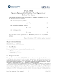
Figure 4: The x-axis shows rbad , the ration of elements that do not belong
to any cluster. The y-axis shows f alse− and f alse+ . n = 300.
In figure (4) there are the plots of f alse− and f alse+ for other k. With
increasing k we notice that the point at which the detection becomes error
prone shifts to the left. As mentioned, this is at least partly due to the
smaller cluster size that results from the fixed n.
An interesting point about this series of plots is that, for rbad greater
than a certain value, the two measures of error rise above 0.5. So more
than half of the elements of each class is actually in the wrong class. This
degeneration of the detection coincides with the collapse of the estimation
of k in ClusterHierarchical. If the eigenvalues of the clusters become
22
to small then not all of them will be accounted for in the estimation of
k. ClusterHierarchical will attempt detection in the belief that there
are less clusters than there are in reality (k 0 < k).
For example, for k = 5 and rbad ≥ 0.7 the estimation of k collapses.
Shortly after that point the values for f alse− and f alse+ rise above 0.5.
It turns out that the estimation of k always collapses before the errors
cross the 0.5 marker.
5.3
Varying p & q
In this experiment we are interested in the effect that varying p and q
have on the detection algorithm ClusterHierarchical. As the threshold
T we use the linear threshold from the previous sections. In all the
experiments from this subsection, rbad is set to 0.4. That means that 40%
of the elements do not belong to clusters. The size of the problem, n, the
number and size of the clusters, and the value for p and q themselves are
varied in the different runs. The actual values are indicated in the label
or the caption of the plot. For every setup of p, q, n, and k, 30 random
experiments have been calculated to average the error.
n=200, k=2, q=1-p
0.6
0.5
0.4
0.3
0.2
0.1
0.0
0.50
0.55
0.60
0.65
0.70
false
_
0.75
0.80
0.85
false +
0.90
0.95
1.00
p
Figure 5: The x-axis shows p, the probability that two elements from the
same cluster are grouped together by the similarity matrix. The y-axis
shows the normalized error. The probability q is set to 1 − p.
In figure (5) we can see the plot of a run, where q = p − 1, starting
from the completely random distribution for D̂ with p = q = 0.5. Then
p is increased in steps of 0.05. Consequently, q is decreased by 0.05, thus
23
increasing p − q by 0.1. If we look at x = p − q, then we find ourselves in
the symmetric situation around 0.5, that is p = 0.5 + x2 and q = 0.5 − x2 .
The plot shows that for p > 0.75 the detection is perfect.
n=200, k=2, q=0.1
0.6
0.5
0.4
0.3
0.2
0.1
0.0
0.50
0.55
0.60
0.65
0.70
false
0.75
_
0.80
0.85
0.90
false +
0.95
1.00
p
Figure 6: The x-axis shows p, the probability that two elements from the
same cluster are grouped together by the similarity matrix. The y-axis
shows the error percentage. The probability q is 1 − p.
The situation in figure (6) is only slightly different. In fact, the only
difference in the choice of the parameters is that here we fix p to 0.1.
The parameter p is again increased by steps of 0.05, starting from 0.5.
It is clear that the error is much smaller for the same value of p, but
in fact if we look at p − q then the setup p = 0.7, q = 0.3 from the
previous run shows slightly better detection than we see in this run with
parameters p = 0.5, q = 0.1. Both parameter choices have p − q = 0.4
though. When the interval between p and q is shifted around from its
centered position around 0.5, then the detection seems to become more
difficult for the same p − q.
+
Finally, in figure (7) you can see f alse−
k and f alsek for different values
of k, namely k ∈ {2, 4, 7}. The ratio of elements that do not belong to
clusters, rbad , is 0.4 for all following choices of parameters. Again, as in
the first series, q = 1−p, and p runs from 0.05 to 1.0 in steps of 0.05. The
size of the problem, n = 60k, depends on k, thus making the problem
size of the k = 7 runs equal to 420.
24
n=60*k, q=1-p, r bad =0.4
0.9
0.8
0.7
0.6
0.5
0.4
0.3
0.2
0.1
0.0
0.50
0.55
0.60
false
_
k=2
0.65
0.70
0.75
0.80
0.85
false+
k=4
0.90
0.95
1.00
p
k=7
Figure 7: The x-axis shows p, the probability that two elements from the
same cluster are grouped together by the similarity matrix. The y-axis
shows the normalized error. The probability q is fixed to 0.1.
In the plot one can see that, in general, an increasing k makes the detection harder. That seems to have something to do with the degeneration
of the linear threshold as in figure (2).
25
6
Conclusion
One of the the main products of this work is the implementation of
the two algorithms ClusterHierarchical and SpectralReconstruct.
With their help one can do the described two-stage clustering of a set
of elements that are characterized by the similarity matrix Â, only exploiting the spectral properties of the matrix, i.e. without knowing k, p,
and q. The algorithm SpectralReconstruct is replaceable by any other
partition reconstruction algorithm. The focus of the experimental work
lay clearly on the evaluation of the algorithm ClusterHierarchical,
with the help of which one can sort out elements that do not belong to
any cluster.
Concerning the algorithm ClusterHierarchical, it is the threshold
value T that is of special interest. The goal was to find out if and how
the threshold depends on the parameters k, p and q. Also, it is of very
practical interest for what ranges of the parameters the method works.
This work proposes a threshold that is a linear function of k. As for the
dependence of p and q we could not find evidence for any. However, the
experiments show the ranges for which the algorithm correctly detects the
elements that should be subjected to the second stage of the clustering
process. Obviously if p gets too small and q to large, or alternatively if
the difference of p and q gets too small, then the detection collapses.
It has to be mentioned that it is not clear yet if the results from the
section about spectral properties apply to the values for n that we used
in the experiments. All the results are asymptotical results for n → ∞,
so it is questionable if we chose a large enough n. However, the results
are satisfactory in the sense that we managed to detect the elements
that belong to clusters for a reasonable range of k, p, and q. Matrices of
moderate size (200 ≥ n ≥ 500) could typically be calculated in the order
of minutes, on a 3.0 GHz Pentium 4, 2GB RAM, personal computer.
The largest matrices (1000 ≥ n ≥ 1200) that we computed took about
half an hour per single matrix, including the random generation of the
matrix.
As for the algorithm SpectralReconstruct, no series of experiments
were conducted, since the computation of the maximum matching that
is needed for the measurement of error is not yet implemented. The algorithm depends on two thresholds that are also derived from asymptotical
considerations, therefore it is not clear to what value they should be set
26
exactly to minimize the error of the planted partition reconstruction.
Manual adjustment of the thresholds showed that it is indeed possible to
achieve a flawless reconstruction of the clusters.
7
Outlook
As already mentioned the next step could be to implement the maximum matching used to measure the error of the reconstruction. Then the
two thresholds of SpectralReconstruct could be scrutinized in order to
come up with practical values that can be substituted for the asymptotical thresholds. Only then will it be possible to assess the whole two-stage
clustering process as described in the introduction.
27
A
Source Code
In this appendix we have included some of the source code of the FASD
program.
Global Variables. First of all, we include the definitions of some
global variables, that will be needed in the following code fragments.
int size = 0; // size of the problem
int nec = 0; // number of eigenvalues needed
double **mat; // variable to store the matrix
double *eval, *evec, *wrk; // workspace for trlan
short *marker; // result of trlan
int
int
int
int
NROW = 0;
LOHI = 1; //computes the ’large’ eigenpairs
MAXLAN = 0;
MEV = 0;
int k = 0; //number of clusters
float p = 0.9f;
float q = 0.1f;
Matrix-Vector Multiplication. The following routine had to be implemented to pass it to TRLAN as an argument. TRLAN requires the
caller to provide his or her own multiplication routine that implements
the multiplication of the stored matrix A with one or more vectors. The
parameters are nRow, the number of rows of A, nCol the number of
columns. xIn and yOut are two one dimensional arrays that are used
to store the vectors to multiply or the resulting vectors respectively. ldx
and ldy are the number if elements in the vectors.
///////////////////////////////////////////////////////////
void mult_vectors(int *nRow, int *nCol, double *xIn,
int *ldx, double *yOut, int *ldy) {
///////////////////////////////////////////////////////////
int i, j, k;
double *xTmp, *yTmp;
for (i=0; i<*nCol; ++i) {
28
yTmp = yOut + *ldy * i;
for (j=0; j<*nRow; ++j, ++yTmp){
xTmp = xIn + *ldx * i;
*yTmp = 0.0f;
for (k=0; k<*nRow; ++k, ++xTmp){
*yTmp += (*xTmp) * ((double)mat[j][k]);
}
}
}
}
Initialization. The following routine initializes the workspace and sets
the maximal relative error that is allowed for the computation of the
eigenpairs. This routine is always called once at the beginning of the
eigenvalue computation.
///////////////////////////////////////////////////////////
void init_TRLan(){
///////////////////////////////////////////////////////////
int i;
for (i=0; i<MEV; ++i) eval[i]=0.0;
for (i=0; i<NROW; ++i) evec[i] = 1.0;
/* relative tolerance on residual norms */
wrk[0] = 1.4901E-8;
}
Stepwise Calculation. The following routine is needed to make use of
the converging computation of TRLAN. Instead of computing all eigenpairs from start, one can define how many eigenpairs are wanted, and
also one can gradually extend the result to more eigenvalues by leaving
the workspace unchanged and call TRLAN again with a request for more
eigenvalues. This is done by this routine. ned specifies the number of
eigenpairs that should be computed, initially set to one. Then, ned is
increased step after step until the absolute value of the next computed
eigenvalue becomes too small.
call TRLan(ned, print) is the call that actually calls the Fortran function.
print is a integer flag that indicates if output to the standard output
should be done or not.
///////////////////////////////////////////////////////////
29
void call_TRLan_gradually(int print){
///////////////////////////////////////////////////////////
int ned = 1;
int tmpK = 1;
float cmp = sqrt(size);
nec = 0;
nec = call_TRLan(ned, print);
if (print) {
printf("%f > nec %d\n", eval[nec - ned - 1], nec);
}
while ((ned <= size) && (nec > 0)
&& (eval[nec - ned - 1] > cmp)) {
tmpK++;
ned++;
nec = call_TRLan(ned, print);
if (print) {
printf("k::::::::::::::::%d\n", tmpK);
printf("%f > nec %d\n", eval[nec - ned - 1], nec);
}
}
k = tmpK;
if (print) {
printf("k:::::::end::::::%d\n", k);
}
}
Interfacing TRLAN. The following function does the call to the Fortran library. ipar is an array of integers to pass all the arguments to the
function call. For an explanation of all the parameters please refer to the
user manual of TRLAN.
///////////////////////////////////////////////////////////
int call_TRLan(int ned, int print){
///////////////////////////////////////////////////////////
if (print) {
printf("\n****************************************\n");
printf("** TRLan\n");
30
printf("****************************************\n");
printf("Matrix loaded: %d x %d\n", size, size);
printf("Starting eigenvalue decomposition...\n\n");
}
int i, j, lwrk, nrow, mev, ipar[32];
double tt, to, tp, tr;
nrow = NROW; mev = MEV;
lwrk = MAXLAN*(MAXLAN+10);
ipar[0] = 0;
ipar[1] = LOHI;
ipar[2] = ned;
ipar[3] = nec; // nec = 0
ipar[4] = MAXLAN;
ipar[5] = 1; // restarting scheme 1
ipar[6] = 2000; // maximum number of MATVECs
ipar[7] = 0; // MPI_COMM
ipar[8] = 10; // verboseness
//Fortran IO unit number for log messages
ipar[9] = 99;
// iguess -- 1 = supply the starting vector
ipar[10] = 1;
// checkpointing flag -- write about -5 times
ipar[11] = -5;
// Fortran IO unit number for checkpoint files
ipar[12] = 98;
// floating-point operations per MATVEC per PE
ipar[13] = 3*NROW;
/* call Fortran function TRLAN77 */
F_TRLAN(mult_vectors, ipar, &nrow, &mev,
eval, evec, &nrow, wrk, &lwrk);
if (print){
printf("\nThe eigenvalues:\n");
for (i=0; i<ipar[3]; i++){
31
printf("E(%i) = %25.17g %16.4e\n", i+1,
eval[i], wrk[i]);
}
// output the k biggest eigenvectors
printf("\nThe %d biggest eigenvectors:\n", ned);
for (j = 0; j < size; ++j){
for (i=ipar[3]-1; i>ipar[3]-ned-1; --i){
printf("%f ", evec[i*size+j]);
}
printf("\n");
}
printf("***************************************\n");
printf("** End of TRLan\n");
printf("***************************************\n\n");
}
return ipar[3]; //return nec
}
32
References
[1] Z. Füredi and J. Komlós. The eigenvalues of random symmetric matrices. Combinatorica I, 3:233–241, 1981.
[2] M. Krivelevich and V. H. Vu. On the concentration of eigenvalues of
random symmetric matrices. Microsoft Technical Report, 60, 2000.
[3] F. McSherry. Spectral partitioning of random graphs. Proceedings of
42nd IEEE Symosium on Foundations of Computer Science, pages
529–537, 2001.
[4] M. Meila and D. Verma. A comparison of spectral clustering algorithms. UW CSE Technical report 03-05-01.
33