Download Thesis Here - Universidade Nova de Lisboa

UNIVERSIDADE NOVA DE LISBOA
Faculdade de Ciências e Tecnologia
Departamento de Engenharia Electrotécnica e Computadores
MICROECG: AN
INTEGRATED PLATFORM FOR THE CARDIAC
ARRYTHMIA DETECTION AND CHARACTERIZATION
Por
Bruno Ricardo Guerreiro do Nascimento
Dissertação apresentada na Faculdade de Ciências e Tecnologia da
Universidade Nova de Lisboa para obtenção do grau de Mestre em Engenharia
Electrotécnica e Computadores
Orientador: Professor Arnaldo Guimarães Batista
Co-orientadores: Professor Manuel Ortigueira
Dr. Luis Brandão Alves
Lisboa
Dezembro, 2009
MicroECG v2.4
2009
Agradecimentos
Esta dissertação não representa só o resultado de extensas horas de estudo, reflexão e
trabalho durante vários anos. É também o culminar de um objectivo académico que me propus e
que não seria possível sem a ajuda de um vasto número de pessoas, entre as quais gostava de
destacar:
O Professor Orientador Arnaldo Batista, ao qual estou profundamente agradecido, não só
pela sua perspicácia, conhecimento e habilidade para superar os diversos obstáculos durante a
orientação desta dissertação, mas também pela constante disponibilidade, amizade e entusiasmo
contagioso.
O Professor Co-orientador Manuel Ortigueira, pelos seus sábios conselhos e recomendações
perante as dificuldades encontradas.
O Professor Raul Rato, pelo interesse e disposição em colaborar sempre que solicitada a sua
ajuda.
O Dr. Luís Brandão Alves do Hospital Garcia de Orta, pela disponibilidade com que nos
recebeu, pelas recomendações apontadas à melhoria do software apresentado e ainda pela
nomeação de pacientes que ajudaram à obtenção de resultados práticos.
Ao Carlos Mendes, pela sua disponibilidade e ajuda no desenvolvimento de versões
anteriores do software aqui apresentado.
Agradeço também à Isabel Couto e Ana Valente, pela ajuda prestada na aquisição dos
electrocardiogramas e por tornarem estas sessões de recolha de dados mais descontraídas.
A todos os voluntários que realizaram o HR-ECG também vai o meu especial apreço pela
paciência e disponibilidade apresentada.
Queria ainda agradecer também a todos os Professores, colegas e amigos que encontrei na
minha passagem pela Faculdade de Ciências e Tecnologia, de quem recebi sempre simpatia e cujos
momentos passados vou sempre transportar comigo.
À minha querida família e à Marta, agradeço, por tudo…
1
MicroECG v2.4
2009
Sumário
O
desenvolvimento
de
um
pacote
de
software
para
lidar
facilmente
com
electrocardiogramas de alta resolução tornou-se importante para pesquisa na área de
electrocardiografia. O desenvolvimento de novas técnicas para detecção de potenciais tardios e
outros problemas associados a arritmias cardíacas têm sido objecto de estudo ao longo dos anos.
No entanto, ainda existe a lacuna de um pacote de software que facilmente permita implementar
algumas destas inovadoras técnicas de uma forma integrada, possibilitando avaliar técnicas
clássicas como o protocolo de Simson para a detecção de sinais não estacionários (potenciais
tardios). Algumas destas inovadoras técnicas envolvem a detecção tempo-frequência usando
escalogramas ou a análise espectral usando metodologias wavelet-packet, sendo implementadas no
software desenvolvido com flexibilidade e versatilidade suficientes para que futuramente sirva de
plataforma de pesquisa para o refinamento destas mesmas técnicas no que toca ao processamento
de sinais de electrocardiogramas de alta resolução. O software aqui desenvolvido foi também
desenhado de forma a suportar dois tipos de ficheiros diferentes provenientes de outros tantos
sistemas de aquisição. Os sistemas suportados são o ActiveTwo da Biosemi e o USBamp da g.tec.
Abstract
The development of a software package able to easily deal with high-resolution
electrocardiograms has became important to the research within the area of electrocardiography.
The development of new late potentials detection techniques and other problems associated to
cardiac arrhythmia have been studied. However, there is still the need of a software package that
can easily implement some of these innovative techniques in an integrated form, allowing the
evaluation of some classic techniques such as the Simson’s protocol to the detection of nonstationary signals (late potentials). Some of these innovative techniques are the time-frequency
analysis through scalograms and the spectral analysis using the wavelet packet methodologies and
they were implemented in the developed software with flexibility and versatility enough to allow, in
the future, that this software could be able to be used as a platform to refine these same techniques
in a signal processing approach. The developed software was designed to support two different data
files from two also different acquisition systems. The supported systems are the Biosemi’s
ActiveTwo and g.tec’s USBamp.
2
MicroECG v2.4
2009
Symbols and connotations’ index
a – Scale
A – Approximation signal
AC – Alternate current
ADC – Analog to digital conversion
AD-Box – Analog to digital Box
AF – Atrial fibrillation
Ag-AgCl – Silver, Silver Chloride
AIB – Analog input box
aVr, aVl and aVf – Extended unipolar derivations
b – Temporal segment
BDF – Biosemi’s data file
𝐛𝐢 (𝐧) - Signal’s noise of n points on the i cycle
BPM – Beats per minute
𝐁𝐰 - Passing band
cA – Approximation signal down sampled
cD – Detail signal down sampled
CMS – Common mode sense
Co2 – Carbon dioxide
CWT – Continuous wavelet transformation
D – Detail signal
DC – Direct current
DI, DII and DIII – Frontal plane bipolar derivations
DRL – Driven right leg
DWT – Discrete wavelet transformation
ECG – Electrocardiogram
ECG(t) – Electrocardiogram in a time domain
EDF – European data format
EEG – Electroencephalography
3
MicroECG v2.4
2009
EMG – Electromyography
EP/ERP – Event potential, event related potential
Fc – Wavelet’s central frequency
FFT – Fast Fourier transformation
Fs - Frequency sampling
HR-ECG – High Resolution Electrocardiogram
𝐇 𝐬 - Transfer function in the s plane
𝐇(𝐰) – Butterworth filter transfer function
H(z) – Transfer function in the z plane
I, II and III – Frontal plane bipolar derivations
IIR - Infinite Impulse Response
LAA – left atrial appendage
LAS – Low amplitude signal
LAS40 – Time duration where the low amplitude signal reaches the 40 microvolts mark until the end of signal
LSB – Least significant bit
M – Length of the signals of reference cycle and signal to align
MEG/MCG – Microgram
mVpp – milliVolts peak to peak
N – Number of cycles (heart beats)
QRSd - QRS complex time duration
QRSoffset – QRS complex end time
QRSonset – QRS complex start time
R – Reference cycle length
RMS – Root mean square
RMS20 – Root mean square value of the last 20 milliseconds
RMS30 - Root mean square value of the last 30 milliseconds
RMS40 - Root mean square value of the last 40 milliseconds
SNR – Signal to noise ratio
RSR – Signal/noise relation
𝐑𝐒𝐑𝐑 – Signal/noise relation in R cycles
S – Signal
4
MicroECG v2.4
2009
s – s plane
s’ = new s plane
𝐬𝐢 (𝐧) - Useful signal of n points on the i cycle
STFT – Short-term Fourier transformation
S-A node – Sino-atrial node
t – Time
V1, V2, V3, V4, V5 and V6 – Unipolar thorax derivations
𝐕𝐀 – Amplitude vector
𝐕𝐋𝐀 – Potential difference in left arm
𝐕𝐋𝐋 – Potential difference in left leg
VLPs – Ventricular Late Potentials
𝐕𝐑𝐀 – Potential difference in right arm
Vx, Vy and Vz – Frank’s derivations
V-A node – Atrio-ventricular node
𝐰𝟎 – Central frequency
xi – Signal of reference cycle
𝐱 – Mean signal
x(t), y(t) and z(t) – Instantaneous amplitudes in the three Frank’s derivations
yi – Signal to align
𝐲 – Reference cycle
z – z plane
Δ - Sampling period of the transformation signal
𝛒 – Correlation
𝛔𝐛 (𝐧) - Standard deviation of the noise’s value on n points
Ψ – Analyzing wavelet
Ψ(t) – Analyzing wavelet in a time domain
Ψ(w) – Fourier transformation of Ψ(t)
5
MicroECG v2.4
2009
Chapter’s Index
1 Objectives …………………………………………………………………………………………….….……….…….pg.13
2 Introduction ………………………………………………………………….…………………………….…….…….pg.14
2.1 Anatomy…………….…………………………………..……………….………..………………….……………….pg.14
2.2 Electrocardiography…………………………………………………….…………..……………………………….pg.15
2.3 The heart’s dynamics ……………………………………………..………………………………………………..pg.15
2.4 Depolarization sequence …………………………………………………..………………………………………pg.16
2.5 Electrical system………………………………..…………………………………………..……………………….pg.17
2.5.1 Electrical pathway ………………………………………………………………………….………………………..pg.18
2.6 Nervous control of the heart ……………………………………………………………………..……..………..pg.18
2.6.1 Accelerator nerves ……………………………………………………………………………….……………….…pg.19
2.6.2 Vagus nerve ……………………………………………………………………………………………..…………….pg.19
2.7 Electrical signal and electrocardiography …………………………………………………………..…….…..pg.19
2.7.1 Standard ECG acquisition: the derivations.……………………………….…………………………..………pg.19
2.7.2 Formation of the ECG signal……………………………………………………………………………….……..pg.22
2.7.3 Vectorcardiography………………………………………………………………………………………………….pg.26
2.8 High Resolution ECG…………………………………………………………………………………………………pg.29
2.8.1 HR-ECG acquisition…………………………………………………………………………………………………..pg.30
2.8.2 Signal Averaging…..………………………………………………………………………………………..………..pg.31
3 Cardiac Arrhythmias…………………………………………………………………………………………….…….pg.35
3.1 Reentrant circuits.…………………………………..……………….……………………………………………….pg.35
3.2 Late potentials…………………………………………………………………………………………………………pg.35
3.2.1 Ventricular arrhythmia and late potentials…..…………………………………………………………..…..pg.36
3.2.2 Atrial arrhythmia and late potentials…..…………………………….……………………………….………..pg.38
4 Late potentials’ detection………………………………………………………………………………..…………pg.40
4.1 Simson’s method..…………………………………..……………….…….…………………….………………….pg.40
4.2 Magnitude vector’s parameters………………………………………………………………………………..…pg.43
5 Late potentials’ detection using wavelets………………………………………………………………………pg.45
5.1 Continuous wavelet transformation…………………………………………………………………………....pg.45
5.2 Discrete wavelet transformation and wavelet packets………………………………………………….…pg.51
6 ActiveTwo system………………………………………………..……………………………………………………pg.55
6
MicroECG v2.4
2009
6.1 Components………………………………….………………………………………………………………………..pg.56
6.2 Technical specifications…………………………………………………………………………………………..pg.61
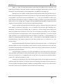
7 Data acquisition…………………………………………………..……………………………………………………pg.62
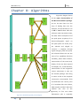
8 Algorithms……………….………………………………..……………………………………………………………pg.64
8.1 General processes…………..…………………………………………………………………………………..…...pg.64
8.2 Late potential simulator…………………………………………………………………………………………….pg.65
8.3 Open file……………………………………………………………………………………………………………...…pg.66
8.4 Read file………………………………………………………………………………………………………………….pg.67
8.5 Peak detection…………………………………………………………………………………………………….…..pg.69
8.6 Show template………………………………………………………………………………………………………..pg.70
8.7 Fine tuning………………………………………………………………………………………………………………pg.70
8.8 ECG variability……………………………………………………………………………………………….………...pg.71
8.9 Heart rate variation………………………………………………………………………………………..…………pg.72
8.10 Noise level………………………………………………………………………………………………….………….pg.72
8.11 Raw data from electrodes…………………………………………………………………………………….…..pg.73
8.12 12-lead ECG…………………………………………………………………………………………………….……..pg.73
8.13 Magnitude vectors…………………………………………………………………………………………………..pg.74
8.14 Wavelets…………………………………………………………………………………………………….………….pg.75
9 Interface…………………………………………….……………………………………………………………………pg.76
9.1 Introduction to MicroECG…………………………………………………………………………………….…….pg.76
9.2 Compilation process………………………………………………………………………………..………………..pg.77
9.3 Installation and minimum requirements…………………………………………………………………….…pg.78
9.4 Instruction manual………………………………………………………………………………………………..….pg.79
10 Results.……………………………………………………………………………………………………………..…pg.109
10.1 Magnitude vectors (Simson’s method for time domain analysis)…………………………………..pg.110
10.2 Heart rate variation……………………………………………………………………………………………..…pg.113
10.3 ECG variability……………………………………………………………………………………………..……….pg.118
10.4 Wavelet scalograms………………………………………………………………………………………………pg.121
10.5 Wavelet packets……………………..………………………………………………………………….…………pg.124
11 Conclusions and further work...………………………………………………………………………………..pg.126
12 References………………………………………………………………………………………………….………..pg.128
7
MicroECG v2.4
2009
Figure’s Index
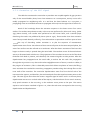
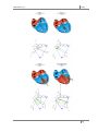
Figure 2.1 - Heart's blood flow…………………………………………………………………………………………………………..………….pg.15
Figure 2.2 - Blood entering the heart……………………………………………………………………………………………………..………pg.15
Figure 2.3 - Atrial contraction……………………………………………………………………………………………………………………….pg.16
Figure 2.4 - Ventricular contraction………………………………………………………………………………………………………..……..pg.16
Figure 2.5 - Human heart in detail. …………………………………………………………………………………………………..…………..pg.17
Figure 2.6 - Heart's electrical system……………………………………………………………………………………………………….…….pg.17
Figure 2.7 - Willem Einthoven (1906)……………………………………………………………………………………………………….…….pg.19
Figure 2.8 - Front plane bipolar derivations…………………………………………………………………………………………….………pg.20
Figure 2.9 - Frontal plane unipolar derivations………………………………………………………………………….……………..……..pg.20
Figure 2.10 - Electrode positioning in the unipolar derivations of the thorax (V1 to V6)……………………..…………….…….pg.21
Figure 2.11 – Sequence of the generation of the ECG signal in the Einthoven limb leads…………………………….…….pg.23/24
Figure 2.12 - The normal electrocardiogram…………………………………………………………………………………………………..pg.25
Figure 2.13 - The projections of the lead vectors of the 12-lead ECG system in three orthogonal planes when one assumes
the volume conductor to be spherical homogeneous and the cardiac source centrally located……………………………..…pg.26
Figure 2.14 - The lead matrix of the Frank VCG-system. The electrodes are marked I, E, C, A, M, F, and H, and their
anatomical positions are shown. The resistor matrix results in the establishment of normalized x-, y-, and z-component
lead vectors, as described in the text………………………………………………………………………………………………………..……pg.27
Figure 2.15 – The seven electrode channels obtained through Biosemi’s ActiveTwo acquisition system using the Frank’s
lead VCG system……………………………………………………………………..…………………………………………………………….…..pg.28
Figure 2.16 – The three Frank’s derivations (Vx, Vy and Vz) obtained in MicroECG by using the seven electrode channels as
input of the Frank’s VCG equation system………………………………………………………………………………………………..…….pg.29
Figure 2.17 - HR-ECG electrode positioning………………………………………………………………………………………….………..pg.31
Figure 2.18 – Noisy signals are often seen even in high quality equipment such as the one used, most of these noise are
due internal factors such as muscular activity or external factors such as environment electromagnetic
noise………………………………………………………………………………………………………………………………………….…………….pg.33
Figure 2.19 – A heart beat template is a smoother signal due to signal averaging………………………………………….……..pg.34
Figure 3.1 - Circuit reentry……………………………………………………………………………………………………………………………pg.35
Figure 3.2 – Historical picture of a patient’s magnitude vector with positive late potentials on QRS Complex.…………..pg.36
Figure 3.3 – MicroECG’s study for the template’s magnitude vector for both the P-wave and the QRS complex. Shown are
ventricular late potentials and their respective parameters values. …………………………………………………………………….pg.37
Figure 3.4 - ECG of atrial fibrillation (top) and sinus rhythm (bottom). The purple arrow indicates a P wave, which is lost in
atrial fibrillation………………………………………………………………………………………………………………………………...………pg.38
Figure 3.5 – MicroECG’s study for the template’s magnitude vector for both the P-wave and the QRS complex. Shown are
atrial late potentials and their respective parameters values…………………………………………………………………………..…pg.39
Figure 4.1 – Bidirectional filter processing an ECG signal. ………………………………………………………….….………………….pg.40
8
MicroECG v2.4
2009
Figure 4.2 - Transfer function and phase of the fourth order Butterworth's passing-band filter. Marked red there is the
passing-band (40 to 250 Hz) on a gain of 0 dB…………………………………………………………………………………………………pg.42
Figure 4.3 - Impulsive response to the fourth order Butterworth filter………………………………………………………..……….pg.42
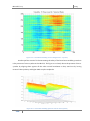
Figure 5.1 - The wavelet-coefficient calculation is illustrated using a set of analyzing wavelet from the ‘Mexican hat’
wavelet and the ECG signal from a healthy subject. The analyzing wavelets are first multiplied by the ECG signal. Then the
wavelet coefficients are calculated using the area under the resulting curves. The area values are then plotted in the timescale domain providing the three-dimensional representation of the signal……………………………………………….………..pg.46
Figure 5.2 - Frequently used wavelet functions in ECG signal processing……………………………………………………………..pg.47
Figure 5.3 - An example of a set of analyzing wavelets from the 2nd Gaussian derivative ('Mexican Hat') is plotted. The
wavelets are represented in both the time (left panel) and the frequency (right panel) domain. The mother wavelet is
drawn with a bold line in the time and frequency domains………………………………………………………………………………..pg.48
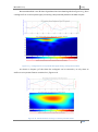
Figure 5.4 – MicroECG obtained scalogram for the P-wave using the detection wavelet: cgau4……………………….……..pg.49
Figure 5.5 – MicroECG obtained scalogram for the P-wave using the detection wavelet: db2……………………………..…..pg.50
Figure 5.6 – MicroECG obtained scalogram for the P-wave using the detection wavelet: fbsp1-1-1…………………….……pg.50
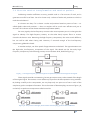
Figure 5.7 – The original signal S, passes through two complementary filters and emerges as two signals…………….….pg.51
Figure 5.8 – The process on the right, which includes downsampling, produces DWT coefficients………………………..…pg.51
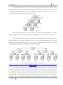
Figure 5.9 – Wavelet decomposition tree………………………………………………………………………………………………..……..pg.52
Figure 5.10 - Wavelet packet decomposition…………………………………………………………………………………………….……pg.52
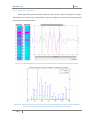
Figure 5.11 – DWT reconstruction and respective values for the coefficients found for an eighth of the available frequency
band width. Only 32 of possible 256 coefficients are shown. The reconstruction of the signal, using all the found
coefficients, when compared with the original signal suffers some degradation……………………………………………………pg.53
Figure 5.12 – DWT reconstruction and respective values for the coefficients found for a quarter of the available frequency
band width. Only 64 of possible 256 coefficients are shown. The reconstruction of the signal, using all the found
coefficients, when compared with the original signal suffers less degradation than the previous
example……………………………………………………………………………………………………………………………………………………pg.54
Figure 6.1 - ActiveTwo System and its components…………………………………………………………………………………………pg.55
Figure 6.2 - Flat-type active-electrodes………………………………………………………………………………………………….……...pg.56
Figure 6.3 - Analog/Digital Box…………………………………………………………………………………………………………………....pg.57
Figure 6.4 - USB2 receiver………………………………………………………………………………………………………..…………………pg.57
Figure 6.5 - ActiView software……………………………………………………………………………………………………………….…….pg.58
Figure 6.6 – Charger……………………………………………………………………………………………………………………………….….pg.59
Figure 6.7 - Battery box………………………………………………………………………………………………………………………………pg.59
Figure 6.8 - Analog Input Box……………………………………………………………………………………………………………………...pg.60
Figure 7.1 - Electrode positions used during the HR-ECG data acquisition (Frank’s leads)………………………………….…..pg.62
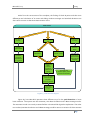
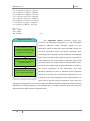
Figure 8.1 – MicroECG’s general process diagram……………………………………………………………………………………….…..pg.64
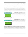
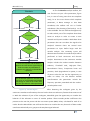
Figure 8.2 – Late potential simulator diagram……………………………………………………………………………………………..….pg.65
Figure 8.3 – Open file diagram………………………………………………………………………………………………………….………….pg.66
Figure 8.4 – Read file diagram……………………………………………………………………………………………………………………..pg.67
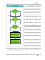
Figure 8.5 – Peak detection diagram……………………………………………………………………………………………………….……pg.69
9
MicroECG v2.4
2009
Figure 8.6 – Show template diagram………………………………………………………………………………………………………..…..pg.70
Figure 8.7 – Fine tuning diagram…………………………………………………………………………………………………………………..pg.70
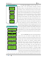
Figure 8.8 – ECG variability diagram……………………………………………………………………………………………………………..pg.71
Figure 8.9 – H.R.V diagram………………………………………………………………………………………………………………………….pg.72
Figure 8.10 – Noise level diagram…………………………………………………………………………………………………………………pg.72
Figure 8.11 – Raw data from electrodes diagram……………………………………………………………………………………….…….pg.73
Figure 8.12 – 12 Lead ECG diagram…………………………………………………………………………………………………………...….pg.73
Figure 8.13 – Magnitude vectors diagram……………………………………………………………………………………………..……….pg.74
Figure 8.14 – Wavelet diagram………………………………………………………………………………………………………………..……pg.75
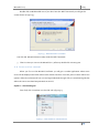
Figure 9.1 - Change "Current Directory"……………………………………………………………………………………………………..….pg.77
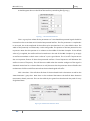
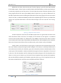
Figure 9.2 - MCRInstaller.exe is present in the given directory………………………………………………………………………..…pg.78
Figure 9.3 - .NET framework is not needed…………………………………………………………………………………………………….pg.79
Figure 9.4 - Click "Simulator" under the File tab…………………………………………………………………………………………..….pg.79
Figure 9.5 - Late Potential Simulator……………………………………………..……………………………………………………………..pg.80
Figure 9.6 - Default beat detection values…………………………………………………………………………………………….……….pg.80
Figure 9.7 – "Automatic” Template…………………………………………….…………………………………………………………………pg.82
Figure 9.8 - Show Template (delineated signal)………………………………………………………………………………………………pg.82
Figure 9.9 - Fine Tuning………………………………………………………………………………………………………………………….…..pg.83
Figure 9.10 - "One Beat Correlation" method………………………………………………………………………………………….………pg.83
Figure 9.11 - "K Beats Average" method………………………………………………………………………………………………….…….pg.84
Figure 9.12 - Open a real acquired signal…………………………………………………………………………………………………….…pg.84
Figure 9.13 - Recent recordings…………………………………………………………………………………………………………………...pg.85
Figure 9.14 - Personal Data, Recording Features………………………………………………………………………………………..……pg.85
Figure 9.15 - Previous recordings……………………………………………………………………………………………………………..…..pg.86
Figure 9.16 - Reading .mat files……………………………………………………………………………………………………………..…….pg.87
Figure 9.17 - Read File group box……………………………………………………………………………………………………………..…..pg.87
Figure 9.18 – Frank’s derivations (Vx, Vy and Vz)…………………………………………………………………………………………….pg.88
Figure 9.19 - Scrolling and zooming through the data………………………………………………………………………………….....pg.88
Figure 9.20 - Heart Rate Variation…………………………………………………………………………………………………………..……pg.90
Figure 9.21 - Raw Data from Electrodes………………………………………………………………………………………………..……….pg.90
Figure 9.22 - Level Noise between Heart Beats (FFT analysis)………………………………………………………………….………..pg.91
Figure 9.23 - Twelve Lead ECG…………………………………………………………………………………………………………….....…..pg.92
Figure 9.24 - ECG Variability………………………………………………………………………………………………………………………..pg.93
10
MicroECG v2.4
2009
Figure 9.25 - ECG Variability (QRS Complex + T Wave / Selected Beats)…………………………………………………………..…pg.94
Figure 9.26 - ECG Variability (QRS Complex + T Wave / All Beats) [Extra-systoles visible]………………………..…………….pg.94
Figure 9.27 - Automatic Template Scenario…………………………………………………………………………………………………...pg.95
Figure 9.28 - Template's Title………………………………………………………………………………………………………………………pg.96
Figure 9.29 - Zoom and Restore Default Viewing………………………………………………………………………………………….…pg.96
Figure 9.30 - Zoomed in templates…………………………………………………………………………………………………………….…pg.97
Figure 9.31 - Magnitude Vectors…………………………………………………………………………………………………………………pg.98
Figure 9.32 - Magnitude Vectors (P-Wave and QRS Complex)……………………………………………………………………..…..pg.98
Figure 9.33 - Magnitude Vectors' Fine Tuning………………………………………………………………………………………………..pg.99
Figure 9.34 - Magnitude Vectors' Results……………………………………………………………………………………………………..pg.99
Figure 9.35 - Wavelet's interface……………………………………………………………………………………………………….………..pg.100
Figure 9.36 - Wavelet Scalogram (default values)……………………..…………………………………………………………………..pg.100
Figure 9.37 - Three wavelet scalogram (P-Wave, QRS Complex and T-Wave)…………………………………………………….pg.101
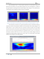
Figure 9.38 - Difference in both scalograms, the right one has a Threshold value of 0.3. The left one has no
Threshold…………………………………………………………………………………………………………………………………………….....pg.101
Figure 9.39 - Wavelet scalogram shows the difference between a filtered signal and a non-filtered signal…………......pg.101
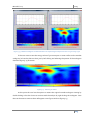
Figure 9.40 - Wavelet scalogram showing the exact same signal, with all the same parameters in different
scales………………………………………………………………………………………………………………………………………………..…...pg.102
Figure 9.41 - Normalization of a wavelet scalogram. From left to right the normalization suffered is 0, 0.5 and
1…………………………………………………………………………………………………………………………………………………………….pg.103
Figure 9.42 - Simulated Late Potential (50:1:300)…………………………………………………………………………………………..pg.103
Figure 9.43 – Different scalogram of a late Potential on an acquired signal. Frequencies used: 1:1:300 and
50:1:300…………………………………………………………………………………………………………………………………………..………pg.104
Figure 9.44 - Selecting an artifact…………………………………………………………………………………………………………..…..pg.104
Figure 9.45 - Nodes and corresponding values of a discrete wavelet transformation of the selected artifact……………pg.105
Figure 9.46 - Save Model……………………………………………………………………………………………………………………….….pg.106
Figure 9.47 - Accessing the "Save Raw Data" feature……………………………………………………………………………..………pg.107
Figure 10.1 - Magnitude vectors for both the P-Wave and the QRS Complex of a healthy subject……………………….…pg.110
Figure 10.2 - Statistical analysis (anoval1) for the values of P-Wave RMS20, 30 and 40 (µV). This procedure could not
differentiate any of these three parameters………………………………………………………………….……………………………….pg.111
Figure 10.3 - Heart rate variation on a healthy subject…………………………………………………………………………………….pg.112
Figure 10.4 - Heart rate variation on a subject that has cardiac extra-systoles…………………………………………………….pg.113
Figure 10.5 - Heart rate variation from a subject suffering from atrial fibrillation…………………………………………………pg.114
Figure 10.6 - Normal P-wave variability…………………………………………………………………………………………………..……pg.116
Figure 10.7 - Normal QRS complex variability………………………………………………………………………………………....……pg.116
Figure 10.8 - Normal T wave variability…………………………………………………………………………………………….…..……...pg.117
11
MicroECG v2.4
2009
Figure 10.9 - Heart Beat Variability (P-wave disappearance)…………………………………………………………………………....pg.117
Figure 10.10 - Heart Beat Variability (P-wave disappearance - top view)……………………………….……………………………pg.118
Figure 10.11 - Heart beat variability (presence of seven extra-systoles)………………………………………………………….….pg.118
Figure 10.12 – Wavelet scalogram on a healthy individual. Detection wavelet used is cmor1-1.5……………………………pg.119
Figure 10.13 – Scalogram showing a simulated late potential using the detection wavelet cmor1-1.5……………..……..pg.120
Figure 10.14 – Scalogram showing a simulated late potential using the detection wavelet fbsp1-1-1………………..……pg.120
Figure 10.15 – Scalogram from an acquired signal showing late potential…………………………………………………..……..pg.121
Figure 10.16 – MicroECG allows zooming in on the late potential artifact………………………………………………………..…pg.121
Figure 10.17 – MicroECG allows the user to extract the coefficients that constitute the late potential artifact….……...pg.122
Figure 10.18 – MicroECG also presents the user a chart containing the RMS and power values of these
coefficients………………………………………………………………………………………………………………………………………………pg.122
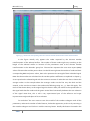
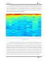
Figure 10.19 – Wavelet packet coefficients from 12 subjects lined side by side, allows seeing the ones suffering from atrial
fibrillation………………………………………………………………………………………………………………………………………………..pg.123
12
MicroECG v2.4
2009
Chapter 1: Objectives
Objectives
One of the major objectives of the development of this software package is that the
MicroECG software could be used as a platform for future studies in cardiac signal processing. To do
this the software package had to be as versatile and flexible as possible, regarding the cardiac
arrhythmia.
The MicroECG software package contains the following features:

Versatile peak detection with wavelets and classical methods

ECG delineation using wavelet methods

Time-frequency analysis through scalogram

Spectral analysis using wavelet packet methodology

Selective reconstruction of the signal in specified frequency bands

Late potential detection using Simson’s method

Heart rate variation

ECG morphology variability

12-lead ECG display

Noise level on ECG’s stationary nodes
13
MicroECG v2.4
2009
Chapter 2: Introduction
2.1 Anatomy
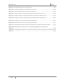
The heart could be described as being 2 pumps. 1 pump (right side) sends blood to your
lungs to be oxygenated and to remove waste products (CO2) and the other pump (left side) sends
the blood around the systemic circulation to oxygenate all the cells in the body. The heart weighs
between 7 and 15 ounces (200 to 425 grams) and is a little larger than the size of your fist; it is
located between your lungs in the middle of your chest, behind and slightly to the left of your
breastbone (sternum).
The heart has 4 chambers. Two upper chambers are called the left and right atria, and the
two lower chambers are called the left and right ventricles. The septum (a wall of muscle) separates
the left and right atria and the left and right ventricles. The left ventricle is known as the largest and
strongest chamber in your heart with enough force to push blood through the aortic valve and into
your body.
The heart chambers have valves which assist in the transport of blood flow through the heart, these
are:

The tricuspid valve regulates blood flow between the right atrium and right ventricle.

The pulmonary valve controls blood flow from the right ventricle into the pulmonary
arteries, which carry deoxygenated blood to your lungs to oxygenate.

The mitral or bicuspid valve lets oxygenated blood from your lungs pass from the left atrium
into the left ventricle.

The aortic valve opens the way for oxygenated blood to pass from the left ventricle into the
aorta, your body's largest artery; from here the blood is distributed to whole of your body.
14
MicroECG v2.4
2009
Figure 2.1 - Heart's blood flow. Extracted from http://www.ambulancetechnicianstudy.co.uk/card.html
2.2 Electrocardiography
In this chapter will be present the fundamental notions of the electrocardiographic genesis
focusing the issue in the high-resolution electrocardiography (HR-ECG). Some of the major
characteristics of the cardiac tissue will be explained as well.
The heart is a muscle made of four major parts; two atrial and two ventricular. The left and
right ventricles push the blood to the pulmonary system and in the systemic blood circulation. Each
heart beat is a mechanical process ruled by bioelectric phenomenon. The excitability and
conductivity are essential properties of the cardiac tissues. These properties vary in their location
inside the myocardial tissues. In periods of activity (systoles) or in periods of rest (diastoles) these
cardiac cells are subjected to a series of complex electrical events on membrane or in intracellular
space. These events have the primary function to promote the fast transmission of electrical
impulses throughout the heart. This electrical activity verification is made through an
electrocardiograph (ECG).
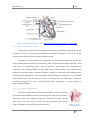
2.3 The heart dynamics
The right and left sides of the heart work together. Firstly, on the right
side of the heart the blood enters the heart through two large veins, the inferior
and superior vena cava, emptying oxygen-poor blood from the body into the
right atrium. The same time, on the left side the pulmonary vein empties
oxygen-rich blood, from the lungs into the left atrium.
Figure 2.2 - Blood
entering the heart.
15
MicroECG v2.4
2009
Then the atrial contraction takes place. On the right side of the heart the
blood flows from the right atrium into the right ventricle through the open
tricuspid valve. When the ventricles are full, the tricuspid valve shuts. This
prevents blood from flowing backward into the atria while the ventricles contract
(squeeze). On the left side the blood flows from the left atrium into the left
ventricle through the open mitral valve. When the ventricles are full, the mitral
Figure 2.3 - Atrial
contraction.
valve shuts. This prevents blood from flowing backward into the atria while the
ventricles contract (squeeze).
The final movement is the ventricular contraction. Again, on the right
side the blood leaves the heart through the pulmonic valve, into the pulmonary
artery and to the lungs. As for the left side the blood leaves the heart through the
aortic valve, into the aorta and to the body.
This pattern is repeated over and over, causing blood to flow continuously
to the heart, lungs and body.
Figure 2.4 - Ventricular
contraction.
Figures extracted from
http://my.clevelandclini
c.org/heart/heartworks/
bloodflow.aspx
2.4 Depolarization sequence
The nerve fibers in their rest condition have fewer number of sodium ions in their inside that
in their outside. This causes an electric tension between the inside and the outside of about 80 to 85
microvolts in the cardiac muscle. After an initial signal, a rapid diffusion of ions occurs on the inside
in a short period of time. This causes a depolarization and inverts the potential. Shortly after, the
sodium ions leave the inside and the membrane is polarized again. This polarization time is known
as refractory period, in which the membrane cannot be depolarized again.
If a depolarization is ignited in a point, it will draw out through the membrane, causing a
muscular contraction, with a speed of about 0.3 to 0.4 m/s to the auricular and ventricular fibers and
till 100 m/s in larger nervous fibers. The refractory period in which the cardiac muscle cannot be
excited is about 0.25 seconds and is known as functional refractory period. Still there is another
relative refractory period that lasts about 0.05 seconds in which is hard, but not impossible to excite
the muscle.
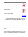
In the right atrium is a small section of specialized muscle called Sino-auricular nodule that
has a low rest potential of about 55 to 60 microvolts and a constant escape of ions. This event causes
a periodic auto-excitation. So each time the rest potential is set, the escape of ions causes a
decrease of potential until the bottom limit is reached in the excitation phase. When this happens,
16
MicroECG v2.4
2009
the Sino-auricular nodule will depolarize.
This depolarization will be transmitted to
both sides of the auricular muscle as it
contracts with a 0.3 m/s velocity. As this
impulse dislocates through the auricular
muscle, it contracts. Given this transmission
velocity the ventricular contraction would
happen before the ventricles are full of
blood, so there is a delay mechanism. The
Figure 2.5 - Human heart in detail. Extracted from
http://www.emergencymedicaled.com/215AED.htm
auricular signal reaches, in 0.04 seconds, to the Auricular-Ventricular nodule, located in the right
atrium, being channelized to the Purkinje fibers, through the bundle of His. These high-velocity
fibers conduct the signal to both ventricles in 2 m/s approximately, where then diminish to a 0.3 m/s.
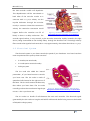
2.5 Electrical System
The electrical system in your heart controls the speed of your heartbeat. Your heart has three
main components to the system, these consist of:

S-A node (sino-atrial node)

A-V node (Atrio-ventricular node)

Purkinje system
The S-A node also called the "natural
pacemaker", of your heart because it controls
your heart rate. The S-A node is made of
specialized cells located in the right atrium of
the heart. The S-A node creates the electricity
that makes your heart beat. The S-A node
normally produces 60-100 electrical signals per
Figure 2.6 - Heart's electrical system. Extracted from
http://www.ambulancetechnicianstudy.co.uk/card.html
minute — this is your heart rate.
The A-V node is a bundle of cells between the atria and ventricles. The electrical signals
generated by the S-A node are "caught" and held for milliseconds before being sent onto the bundle
of HIS (HIS Purkinje system).
17
MicroECG v2.4
2009
HIS-Purkinje system is in your heart's ventricles. Electricity travels through the His-Purkinje
system to make your ventricles contract. The electricity from the A-V node hits the bundle of HIS
before being directed into the right and left bundle branches and finally into the Purkinje fibers that
are located in the cardiac muscle. This stimulates the ventricles to contract.
2.5.1 Electrical Pathway
1. The S-A node creates an electrical signal
2. The electrical signal follows natural electrical pathways through both atria. The movement
of electricity stimulates the atria to contract, which pushes blood into the ventricles.
3. The electrical signal reaches the A-V node. There, the signal pauses to give the ventricles
time to fill with blood
4. The electrical signal spreads through the His-Purkinje system. The movement of electricity
causes the ventricles to contract and push blood out to your lungs and body.
The name for the steps above is known as the cardiac cycle which lasts for 0.8 seconds:

Atrial systole = 0.1 second

Ventricular systole = 0.3 seconds

Diastole = 0.4 seconds
(Systole refers to the contraction of the cardiac muscle; Diastole refers to the relaxation of the
cardiac muscle)
2.6 Nervous Control of the Heart
Although the S-A node sets the basic rhythm of the heart, the rate and strength of its beating
can be modified by two auxiliary control centers located in the medulla oblongata of the brain.

One sends nerve impulses down accelerator nerves.

The other sends nerve impulses down a pair of Vagus nerves
18
MicroECG v2.4
2009
2.6.1 Accelerator Nerves
The accelerator nerves are part of the sympathetic branch of the autonomic nervous system.
They increase the rate and strength of the heartbeat and thus increase the flow of blood. Their
activation usually arises from some stress such as fear or exertion. The heartbeat may increase to
180 beats per minute. The strength of contraction increases as well so the amount of blood pumped
may increase to as much as 25-30 liters/minute.
2.6.2 Vagus Nerve
The Vagus nerves are part of the parasympathetic branch of the autonomic nervous system.
They, too, run from the medulla oblongata to the heart. Their activity slows the heartbeat. Pressure
receptors in the aorta and carotid arteries send impulses to the medulla which relays these impulses
back by way of the Vagus nerves to the heart. Heartbeat and blood pressure diminish.
2.7 Electric signals and electrocardiography
One electric fiber in depolarization may be compare to a current dipole.
On a given instant, the activation wave’s front formed by elementary dipoles
creates an electric field in result of the dipolar moments. The time evolution
registry of the electrical field is made through coetaneous electrodes is called
electrocardiogram.
Electrocardiography is about 100 years old and coincides with the
creation of the first registry system sensitive enough to measure the cardiac
electrical potentials from the surface of the body. This system was first
developed in 1903 by the Dutch Doctor Willem Einthoven [Einthoven, 1903]. He
Figure 2.7 - Willem
Einthoven (1906).
Extracted from
http://pt.wikipedia.or
g/wiki/Willem_Eintho
ven
was awarded the Nobel Prize of Medical or Physiological Achievements in 1924.
2.7.1 Standard ECG acquisition: the derivations
A derivations system, in electrocardiography, consists in a coherent set of electrode
locations, each one defined by their positions on the patient’s thorax. The positioning of the
electrodes is chosen on a way to cover the cardiac electrical potential through a set of nonredundant derivations. There are several standard systems. Now will be explained the most used
systems in chronological order and what kind of electrocardiograms they are most associated.
19
MicroECG v2.4
2009
Frontal plane bipolar derivations
The bipolar derivations DI, DII and DIII explore the cardiac
activity in a frontal plane. This referential system is limited by an
equilateral triangle (Einthoven Triangle). The three electrodes are
placed respectively in the right arm (RA), on the left arm (LA) and
on the left leg (LL). It is considered to all vectors to be
instantaneous and have a common origin in the triangle’s center
and is projections are obtained through its sides, measuring the
electric tension between the points:
𝐷𝐼 = 𝑉LA − VRA
(2.1)
𝐷𝐼𝐼 = 𝑉LL − VRA
(2.2)
𝐷𝐼𝐼𝐼 = 𝑉LL − VLA
(2.3)
Figure 2.8 - Front plane bipolar
derivations
And have the relation:
𝐷𝐼 + 𝐷𝐼𝐼𝐼 = 𝐷𝐼𝐼
(2.4)
Frontal plane unipolar derivations
In 1934, Wilson introduced the unipolar derivations.
[Kossman 1985] In this case the electric tension is measured
between a point of reference and each one of the R, L, and F
points. In this system the referential point is designed by
“Wilson’s Central Electrode” which is a virtual point and
supposedly has a null differential potential.
Goldberger [Goldberger 1942] proposed in 1942, the
extended unipolar derivations (aVr, aVl and aVf). These
derivations allow the acquisition of greater amplitude signals
then the Wilson method. These derivations measure the
Figure 2.9 - Frontal plane unipolar
derivations. Figures extracted from
Biomedical Digital Signal Processing,
Tompkins, pg.38 [Tompkins 1993]
potential difference between each one of the three (RA, LA and LL) points and the mean potential
from the other two. This way the electric tension is increased in a factor of 1.5 in comparison to the
Wilson’s derivations.
20
MicroECG v2.4
𝑎𝑉𝑟 = 𝑉𝑅𝐴−
𝑉𝐿𝐴 −𝑉𝐿𝐿
2
2009
(2.5)
𝑎𝑉𝑙 = 𝑉𝐿𝐴 −
𝑉𝐿𝐿 −𝑉𝑅𝐴
2
(2.6)
𝑎𝑉𝑓 = 𝑉𝐿𝐿 −
𝑉𝑅𝐴 −𝑉𝐿𝐴
2
(2.7)
In 1935 Kossman proposed the unipolar thorax derivations (v1 to v6). These six unipolar
derivations run the precordial region and the left lateral transversally. They correspond to the
electric tension between each electrode and the “Wilson’s Central Electrode”.
Figure 2.10 - Electrode positioning in the unipolar derivations of the thorax (V1 to V6). Extracted from
http://www.bem.fi/book/15/15.htm [Malmivuo 1995]
21
MicroECG v2.4
2009
2.7.2 Formation of the ECG signal
The cells that constitute the ventricular myocardium are coupled together by gap junctions
who, for the normal healthy heart, have a low resistance. As a consequence, activity in one cell is
readily propagated to neighboring cells. It is said that the heart behaves as a syncytium; a
propagating wave once initiated continues to propagate uniformly into the region that is still at rest.
Much of the knowledge about the activation sequence in the heart comes from canine
studies. The earliest comprehensive study in this area was performed by Scher and Young. [Scher
1957] More recently, such studies were performed on the human heart, and a seminal paper
describing the results was published by Durrer [Durrer 1970]. These studies show that activation
wave fronts proceed relatively uniformly, from endocardium to epicardium and from apex to base.
One way of describing cardiac activation is to plot the sequence of instantaneous
depolarization wave fronts. Since these surfaces connect all points in the same temporal phase, the
wave front surfaces are also referred to as isochrones. After the electric activation of the heart has
begun at the sinus node, it spreads along the atrial walls. The resultant vector of the atrial electric
activity is illustrated with a thick arrow. The projections of this resultant vector on each of the three
Einthoven limb leads is positive, and therefore, the measured signals are also positive. After the
depolarization has propagated over the atrial walls, it reaches the AV node. The propagation
through the AV junction is very slow and involves negligible amount of tissue; it results in a delay in
the progress of activation. (This is a desirable pause which allows completion of ventricular filling.)
Once activation has reached the ventricles, propagation precedes along the Purkinje fibers to the
inner walls of the ventricles. The ventricular depolarization starts first from the left side of the
interventricular septum, and therefore, the resultant dipole from this septal activation points to the
right. The next figures show that this causes a negative signal in leads I and II. In the next phase,
depolarization waves occur on both sides of the septum, and their electric forces cancel. However,
early apical activation is also occurring, so the resultant vector points to the apex. This events
sequence can be better visualized in figures 2.11, where the red zones correspond to the occurring
depolarization and depolarization.
22
MicroECG v2.4
2009
23
MicroECG v2.4
2009
Figures 2.11 – Sequence of the generation of the ECG signal in the Einthoven limb leads. Figures extracted from
http://www.bem.fi/book/15/15.htm [Malmivuo 1995]
24
MicroECG v2.4
2009
After a while the depolarization front has propagated through the wall of the right ventricle;
when it first arrives at the epicardial surface of the right-ventricular free wall, the event is called
breakthrough. Because the left ventricular wall is thicker, activation of the left ventricular free wall
continues even after depolarization of a large part of the right ventricle. Because there are no
compensating electric forces on the right, the resultant vector reaches its maximum in this phase,
and it points leftward. The depolarization front continues propagation along the left ventricular wall
toward the back. Because its surface area now continuously decreases, the magnitude of the
resultant vector also decreases until the whole ventricular muscle is depolarized. The last to
depolarize are basal regions of both left and right ventricles. Because there is no longer a
propagating activation front, there is no signal either.
Ventricular repolarization begins from the outer side of the ventricles and the repolarization
front "propagates" inward. This seems paradoxical, but even though the epicardium is the last to
depolarize, its action potential durations are relatively short, and it is the first to recover. Although
recovery of one cell does not propagate to neighboring cells, one notices that recovery generally
does move from the epicardium toward the endocardium. The inward spread of the repolarization
front generates a signal with the same sign as the outward depolarization front. Because of the
diffuse form of the repolarization, the amplitude of the signal is much smaller than that of the
depolarization wave and it lasts longer.
The normal electrocardiogram is
illustrated in figure 2.12. The figure also
includes definitions for various segments
and intervals in the ECG. The deflections in
this signal are denoted in alphabetic order
starting with the letter P, which represents
atrial
depolarization.
The
ventricular
depolarization causes the QRS complex,
and repolarization is responsible for the Twave. Atrial repolarization occurs during
the QRS complex and produces such low
signal amplitude that it cannot be seen
apart from the normal ECG.
Figure 2.12 - The normal electrocardiogram. Extracted from
http://www.bem.fi/book/15/15.htm [Malmivuo 1995]
25
MicroECG v2.4
2009
2.7.3 Vectorcardiography
It was still in 1914 that Williams first came up with the concept of Vectorcardiography.
Williams [Williams 1914] proposed a representation of the cardiac signal in four dimensions, time
and space in three dimensions, comprehending the frontal sagittal, and transverse plane of the
human body, as seen on figures 2.13. Vectorcardiography is based on the theory of the unique dipole
through which all information about the cardiac activity manifests, on a given instant, through the
form of an electric field vector with the origin, on the 0 point, which represents the electric center of
the ventricular mass. This 0 point is fixed and is utilized as the point of origin of all resulting
instantaneous vectors that evolve through time.
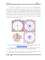
Figure 2.13 - The projections of the lead vectors of the 12-lead ECG system in three orthogonal planes when one
assumes the volume conductor to be spherical homogeneous and the cardiac source centrally located. Extracted
from http://www.bem.fi/book/15/15.htm [Malmivuo 1995]
Each sequence of the cardiac electric field, P, QRS and T may be represented by a set of
successive of resulting vectors and constitute a spatial curve named vectorcardiogram.
Frank, in 1956, utilized a system of derivations in X, Y and Z with clinical applications and it is
still today, one of the most used vectorcardiographic systems. [Frank 1956]
26
MicroECG v2.4
2009
It was this vectorcardiographic system used in the data recording sessions to obtain the
three Frank’s derivations because of his correct orthogonal system since allows to see the changes in
morphology in a spatial orientation.
All three Frank’s derivations are obtained through a network of resistors that linearly
combine all potentials obtained through eight coetaneous electrodes, as seen on figure 2.14.
This system must still be normalized. Therefore, resistors 13.3R and 7.15R are connected
between the leads of the x- and y-components to attenuate these signals to the same level as the zlead signal. Now the Frank lead system is orthogonal.
It should be noted once again that the resistance of the resistor network connected to each
lead pair is unity. This choice results in a balanced load and increases the common mode rejection
ratio of the system. The absolute value of the lead matrix resistances may be determined once the
value of R is specified. For this factor Frank recommended that it should be at least 25kΩ, and
preferably 100 kΩ. Nowadays the lead signals are usually detected with a high-impedance
preamplifier, and the lead matrix function is performed by operational amplifiers or digitally
thereafter. Figure 14 illustrates the complete Frank lead matrix.
It is worth mentioning that the Frank system is presently the most common of all clinical
VCG systems throughout the world. (However, VCG's represent less than 5% of the
electrocardiograms.).
Figure 2.14 - The lead matrix of the Frank VCG-system. The electrodes are marked I, E, C, A, M, F, and H, and their
anatomical positions are shown. The resistor matrix results in the establishment of normalized x-, y-, and zcomponent lead vectors, as described in the text.
27
MicroECG v2.4
2009
The referential system is a tri-orthogonal rearrange where all axes are adapted to the
geometry of the thorax; OX transverse, OY frontal and OZ sagittal. The signals registered in X, Y and
Z is the projections of the instantaneous vectors over all three axes. This way V x, Vy and Vz are given
by:
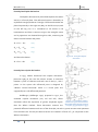
𝑉𝑋 = 0.61𝑉𝐴 + 0.171𝑉𝐶 − 0.781𝑉𝐼
(2.8)
𝑉𝑌 = 0.655𝑉𝐹 + 0.345𝑉𝑀 − 1𝑉𝐻
(2.9)
𝑉𝑍 = 0.133𝑉𝐴 + 0.736𝑉𝑀 − 0.264𝑉𝐼 − 0.374𝑉𝐸 − 0.231𝑉𝐶
(2.10)
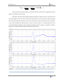
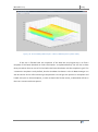
These equations are used in the developed software package to transform the obtained VCG
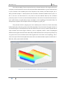
signal into the three Frank’s derivations. As seen from figure 2.15 the seven channels obtained , in
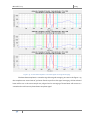
MicroECG, through the VCG recording sessions are inputs for these equations. The result can be
seen on figure 2.16 as the three Frank’s derivations are obtained by MicroECG.
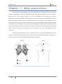
Figure 2.15 – The seven electrode channels obtained through Biosemi’s ActiveTwo acquisition system using the
Frank’s lead VCG system.
28
MicroECG v2.4
2009
Figure 2.16 – The three Frank’s derivations (Vx, Vy and Vz) obtained in MicroECG by using the seven electrode
channels as input of the Frank’s VCG equation system. (Equations 2.8, 2.9 and 2.10)
2.8 High-resolution electrocardiogram (HR-ECG)
High-resolution electrocardiography is considered to be a recent technique that only in 1972
was described for the first time in terms of signal analysis. [Evanich 1972] The high-resolution ECG is
a method that allows increasing the signal/noise relation of the electrocardiogram. This method is
largely used to register the transitory cardiac signals with low amplitude and high frequency,
impossible to detect on a classic electrocardiogram. The utilization of the signal averaging is a
method that supports on the fact of the electrocardiographic signal repeats itself on each cardiac
cycle. By making the average over the number of N cycles (N [50,300]), allows to reduce quite
significantly the noise in a 1/ 𝑁 reason, with the conservation of the information that are
synchronous in each cycle.
29
MicroECG v2.4
2009
The calculation of the ECG average needs a pre-treatment to detect and align the successive
heart beats.
The quality of the electrocardiographic registry is dependent of the acquisition system, from
the sampling frequency and from the presence of electrical and magnetic interferences. The
electrical interference of muscular origin is a very important component of the interference and it is
very hard to eliminate.
The presence of interferences induces a fundamental problem in high-resolutionelectrocardiography because the noise is constituted by low amplitude, high frequency signals,
much as the late potentials that appears on post-stroke patients or with tachycardia problems. For
the needed precision, the technical characteristics of classical registry systems (gain, amplitude
resolution, sampling frequency, etc) are general case, insufficient.
A possible application of the HR-ECG it is his utilization on the detection of late potentials on
patients that suffered myocardium infraction. [Gomes 1972] On the late 1970’s, a common and
growing interest on the comprehension of the mechanisms that generate ventricular arrhythmias
conduct to the study of abnormal mechanisms on the ventricular depolarization, specifically on the
QRS complex. The most notable study that still holds as a reference to this domain is the work of
Simson that showed the relation between the presences of late potentials and the risk of ventricular
tachycardia. On the sequence of Simson’s work, many more followed, however the methods of
acquisition and pre-treatment were so diversified that all the results became practically impossible
to compare. So in order to standardize this method an international consensus was created,
suggesting some norms over the acquisition techniques and processing of the HR-ECG data.
[Breithardt 1991]
2.8.1 HR-ECG acquisition
The first generation of high-resolution electrocardiographic devices was limited to analog
acquisition systems, however since 1979, digital acquisitions systems became present that allowed
to a, posterior, digital treatment of the results, that weren’t possible before.
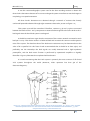
The positioning of the electrodes in the acquisition of the HR-ECG was the matter of
discussion and an international consensus was established, recognizing that the utilization of the
three pseudo-orthogonal derivations positioned as present on the figure 2.17. Still, until today, no
study was able to determinate a positioning of the electrodes that allow an optimum measure of
these late potentials.
30
MicroECG v2.4
2009
Figure 2.17 - HR-ECG electrode positioning.
The quality of the skin/electrode interface should be optimum. Ag/AgC electrodes are
normally used, since they are the most accurate for standard registration, however no study to date,
verified this matter for the HR-ECG.
The gain in the amp of these acquisition system is normally fixed somewhere on 1000 to
8000 for frequencies comprehended on 0.5 to 300 Hz, but this value depends on the analog/digital
converter’s resolution.
2.8.2 Signal Averaging
After the amplification and analog filtering, the signal will be digitalized. The AD-Box was
used with the following settings on the new recording sessions; a 2048 Hz sampling frequency and
the amplitude of the signal was codified on a 24 bit with a 31nV resolution (LSB).
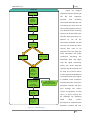
The detection of the QRS complexes (R points) should be made in three steps:
1. A IIR (Infinite Impulse Response) 1st order Butterworth filter is applied on a passing band
between 5 and 30 Hz, to avoid tension fluctuations across the QRS complex and to eliminate
DC components introduced by the skin/electrode interface e mainly because the largest part
of the energy of the QRS complex’s signal is found on the passing band referred.
2. An algorithm is applied, that detects relative maximum points over a given “threshold”
value, on the filtered signal.
3. Because filtering always causes a displacement of the signal, another algorithm to detect
the relative maximum point of the original signal. This way the R point for each heart cycle is
captured for the three Frank’s derivations.
31
MicroECG v2.4
2009
After the detection step, the classification of the QRS complexes is essential part of the
process, to exclude the noisy heart beats. In HR-ECG the selection of the QRS complexes is made
through an algorithm that uses a value of correlation between the complex to analyze and a
complex of reference. The recommended value to the coefficient is generally superior to 0.95.
The synchronization of the complexes is made through a function of correlation calculated
between each QRS complex of a heart beat and a QRS complex of reference. This synchronization
should apply to all the cardiac cycle and not just the QRS complex, because the study of the P wave
is also important. The correlation coefficient is given by the equation:
𝜌=
𝑀
𝑖=1 𝑥 𝑖 𝑦 𝑖
𝑀
2
𝑖=1 𝑥 𝑖
𝑀
2
𝑖=1 𝑦 𝑖
(2.11)
Where xi and yi are respectively the M values that constitute the signal of the reference cycle
and the signal to align. A minimum value of correlation accepted was established on 0.97 in with is
considered an acceptable synchronization. In practice and after the study of Lander, the value of this
correlation was set between 0.95 and 0.99. [Lander 1992]
The reference cycle 𝑦(𝑛) is given by:
𝑦 𝑛 =
𝑅
𝑖=1 𝑥 𝑖 (𝑛)
𝑅
(2.12)
The calculation of the mean signal 𝑥 (𝑛) of R cycles is given by:
𝑥 𝑛 =
𝑅
𝑖=1 𝑥 𝑖 (𝑛 )
𝑅
=
𝑅
𝑖=1 𝑠𝑖 (𝑛 )
𝑅
+
𝑅
𝑖=1 𝑏 𝑖 (𝑛 )
𝑅
(2.13)
Where 𝑥𝑖 (𝑛) represents all the electrocardiographic signal and 𝑠𝑖 (𝑛) and 𝑏𝑖 (𝑛) are,
respectively, the useful signal and the signal’s noise of n points on the i cycle. The origin of n is found
relatively to a point of synchronization linked to the useful signal.
The signal/noise relation (RSR) is defined by the module of the signal over the noise’s power:
𝑅𝑆𝑅 =
𝑠(𝑛 )
𝜎𝑏 (𝑛)
(2.14)
Where 𝜎𝑏 (𝑛) is the standard deviation of the noise’s value on n points. This signal/noise
relation in R cycles 𝑅𝑆𝑅𝑅 is:
32
MicroECG v2.4
2009
𝑆𝑅𝑅 =
𝑅 𝑠(𝑛 )
𝑅𝜎 2 (𝑛 )
=
𝑅 𝑠(𝑛)
𝑅𝜎𝑏 (𝑛 )
= 𝑅𝑆𝑅 𝑅
(2.15)
The conclusion of this last equation is that the reduction of the noise is proportional to the
square root of the number of cycles.
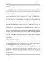
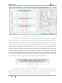
MicroECG uses these same signal averaging principles to reduce the noise in the signal. This
signal averaging process will not only obtain a template signal of the systematic heart beat signal
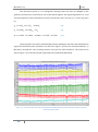
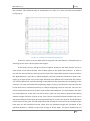
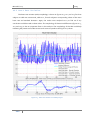
but will also decrease the template’s noise. This noise present in the acquired data, as seen on figure
2.18 is often attributed to internal factors such as muscular activity or to external factors such as
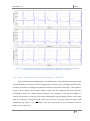
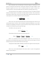
environment electromagnetic noise. The signal’s template, as seen on figure 2.19, will be a “cleaner”
signal than a random heart beat selected from the acquired data.
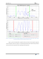
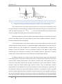
Figure 2.18 – Noisy signals are often seen even in high quality equipment such as the one used, most of these noise
are due internal factors such as muscular activity or external factors such as environment electromagnetic noise.
33
MicroECG v2.4
2009
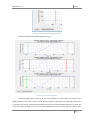
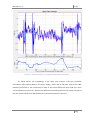
Figure 2.19 – A heart beat template is a smoother signal due to signal averaging.
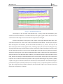
The heart beat template is a smoother signal due signal averaging. As seen in the figure 2.19
the template uses around 280 of 300 beats found to perform this signal averaging. All the selected
beats will be cut in the same sample size, aligned and an averaging of these beats will construct a
smooth and much less noisy heart beats’ template signal.
34
MicroECG v2.4
2009
Chapter 3: Cardiac Arrhythmias
3.1 Reentrant circuits
Arrhythmias could be generated by several distinct mechanisms, however the one most
associated with the appearance of late potentials is the reentrant circuit mechanism. This is the
most common mechanism and is due to the existence of unidirectional blockage of ways or paths in
the heart that facilitate the start and maintenance of these mechanisms. The reentrant arrhythmias
are generally induced by atrial or ventricular ectopic heart beats that could be ignited by excessive
injection of caffeine or alcohol.
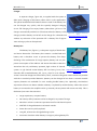
Figure 3.1 shows the electric flow as it
reaches the A, B base and divides in two. On A the flow is
detained by a non susceptible zone to depolarization. On B
the flow heads for the C trench, only to propagate after to A
again, on reverse, where originates a re-excitation of the
heart tissues.
Figure 3.1 - Circuit reentry. Extracted
from Slama, "Aide mémoire de la
rythmologie", pg. 26 [Slama 1987]
3.2 Late Potentials
Late potentials are scattered, low-amplitude and abnormal micro-potentials, (about 25
microvolts in amplitude) due to reentrant circuit activity. The first study to observe the presence of
late potentials realized on a dog, after a myocardium infraction, was performed by Boineau and Cox.
[Boineau 1973] Then a study by Williams showed that late potentials are markers of the presence of
reentries capable of generate ventricular arrhythmia. Just in 1986, Kuchar [Kuchar 1986]
demonstrated that only patients that conserve these late potentials several days after the
myocardium infraction are suitable to suffer ventricular tachycardia or even sudden death.
So, cardiac late potentials are low amplitude signals that occur in the ventricles. Also called
Ventricular Late Potentials (VLPs), these signals are caused by slow or delayed conduction of the
cardiac activation sequence. Under certain abnormal conditions, there may be small regions of the
ventricles within a diseased or ischemic region that generate such delayed conduction. This results
in depolarization signals that prolong past the refractory period of surrounding tissues and re-excite
the ventricles. This re-excitement is known as 'reentry'. Reentry is believed to be a key factor that
causes VLPs.
35
MicroECG v2.4
2009
Due to their very low magnitudes, late potentials are not visible in a standard ECG.
Moreover, factors such as increased distance of the body surface electrodes from the heart, and
inherent noise in patients make identification of VLPs beyond the resolution limits of a standard
ECG. As a result, high-resolution recording techniques and computerized ECG processing are
necessary for detection of late potentials. Figure 3.2 shows an historical figure where the patients’
magnitude vector clearly shows VLPs on the QRS complex signal. ECG signal processing includes
techniques to improve the signal-to-noise ratio (SNR). One widely used technique to improve the
SNR of ECG signals for the detection of late potentials is signal averaging.
Figure 3.2 – Historical picture of a patient’s magnitude vector with positive late potentials on QRS Complex. Figure
extracted from http://cogprints.org/4314/1/hrecg.htm
3.2.1 Ventricular Arrhythmia and late potentials
The most common application of the HRECG is to record very low level (~1.0-μV) signals
that occur after the QRS complex but are not evident on the standard ECG. These “late potentials”
are generated from abnormal regions of the ventricles and have been strongly associated with the
substrate responsible for a life-threatening rapid heart rate (ventricular tachycardia).
In the last years, the ventricular late potentials detection has been used to study the conduction
disturbances in the cardiac ventricles. The ventricular late potentials are composed by high
frequency and low amplitude signals that occur in the last portion of the QRS complex and/or in the
36
MicroECG v2.4
2009
beginning of the ST segment. It was postulated that these late potentials would constitute noninvasive markers of the presence of an arrhythmogenic subtract, characterized by a slow and nonhomogeneous propagation of the intraventricular activation wave.
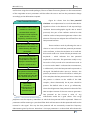
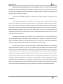
MicroECG does this magnitude vector study from the template obtained from signal
averaging. As figure 3.3 shows the magnitude vectors are split in two charts; the upper greendelineated chart is corresponding to the P-wave magnitude vector as for the lower red-delineated
chart corresponds for the QRS complex magnitude vector. Both charts are shown similarly to the
historical figure 3.2 in µV / ms. As the historical figure 3.2 only shows only parameters corresponding
to the QRS Complex, MicroECG is capable of studying both magnitude vectors because there are a
series of parameters shown below the charts that correspond to the P-wave and the QRS complex.
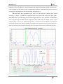
Figure 3.3 – MicroECG’s study for the template’s magnitude vector for both the P-wave and the QRS complex. Shown
are ventricular late potentials and their respective parameters values.
37
MicroECG v2.4
2009
Note that in figure 3.3 the parameters used for the magnitude vector study and their
nominal values are known for the QRS complex case. However, no particular parameters or nominal
values are known for the P-wave study. In chapter 4 there is a more elaborate explanation of what
this parameters and their nominal values stand for.
3.2.2 Atrial arrhythmia and late potentials
Atrial fibrillation is often asymptomatic, and is not in itself generally life-threatening, but
may result in palpitations, fainting, chest pain, or congestive heart failure. People with AF usually
have a significantly increased risk of stroke (up to 7 times that of the general population). Stroke risk
increases during AF because blood may pool and form clots in the poorly contracting atria and
especially in the left atrial appendage (LAA). The level of increased risk of stroke depends on the
number of additional risk factors. If a person with AF has none, the risk of stroke is similar to that of
the general population. However, many people with AF do have additional risk factors and AF is a
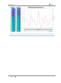
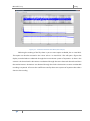
leading cause of stroke. Figure 3.4 show how the P-wave signal is made invisible with severe atrial
fibrillation patients.
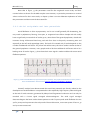
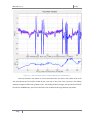
Figure 3.4 - ECG of atrial fibrillation (top) and sinus rhythm (bottom). The purple arrow indicates a P wave, which is
lost in atrial fibrillation. Extracted from http://en.wikipedia.org/wiki/Atrial_fibrillation
Scientific studies have demonstrated that atrial late potentials are directly related to the
development of atrial fibrillation. Late potentials are low amplitude, high frequency electrical signals
at the end of atrial activation, generated by delayed and fragmented conduction and can only be
recorded with a P-wave signal averaged electrocardiogram. The atrial signal averaged
electrocardiogram has been used to detect patients at risk for paroxysmal atrial fibrillation but not
yet for paroxysmal supraventricular tachycardia. The atrial duration, root mean square of last 20, 30
and 40 ms were measured.
38
MicroECG v2.4
2009
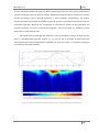
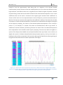
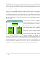
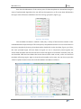
Figure 3.5 – MicroECG’s study for the template’s magnitude vector for both the P-wave and the QRS complex. Shown
are atrial late potentials and their respective parameters values.
Figure 3.5 shows how MicroECG is capable to detect and show VLPs through the magnitude
vectors calculated. Present in the figure is a simulated late potential. Also visible are the parameters
used to quantify these magnitude vectors regarding the late potentials.
39
MicroECG v2.4
2009
Chapter 4: Late potentials’
detection
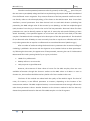
This chapter describes the conventional method for late potentials’ detection through the
electrocardiogram’s signal averaging.
The various stages in the HR-ECG analysis in time domain are the detection, alignment, and
filtering of the QRS complexes. The pass-band filtering should have cut-frequencies from 25, 40 or
80 until 250 Hz to isolate late potentials.
4.1 Simson’s method
The most utilized method to establish a prognosis of the post-infraction ventricular
tachycardia was created by M.B. Simson in 1981.
Simson [Simson 1981] proposed
an original method using IIR filters, so that
the “ringing” phenomenon is eliminated in
the
use
of
a
bidirectional
filtering
technique. “Ringing” consists in the
transitory response that usually happens
when a signal, that varies abruptly, is
submitted to a filter. It is the equivalent to
the oscillation of a body when submitted
to an abrupt mechanical excitation. This
phenomenon
is
undesirable
as
it
constitutes a source of distortion. The HRECG is filtered from the P-Wave in
direction to the QRS complex and then
from the ST segment in direction to the
Figure 4.1 – Bidirectional filter processing an ECG signal.
Extracted from “A Practical Guide to High-Resolution
Electrocardiogram”, Berbari, pg. 49 [Berbabri 2000]
QRS complex. The utilized filter is a four-pole Butterworth filter with a passing-band between 40
and 250 Hz. Figure 4.1 show how the bidirectional filter uses the filter formula starting from both the
left and the right side of the top of the signal, a signal averaged Z lead. The fiducial point is in the
40
MicroECG v2.4
2009
mid-QRS region. The bottom trace is filtered output in the forward time sense from the left side and
the reverse time sense from the right side.
By applying the filter in a bidirectional fashion, the significant time shift of QRS energy is
confined to the middle of the QRS complex and minimally distorts the timing relationship between
the QRS endpoints and the late potentials. As it was noted in a previous chapter, the late potentials
have higher frequency content than the QRS and ST segments.
The creation of the fourth order prototype filter involves the setting of a low-pass analog
filter. Since the filter is a forth order, four poles will be obtained and the transfer function can be
represented has:
𝐻 𝑠 =
𝑍(𝑠)
𝑃(𝑠)
=
𝑘
𝑠−𝑝 1 . 𝑠−𝑝 2 …(𝑠−𝑝 𝑛 )
(4.1)
To a Butterworth filter, the squared transfer function, H (w) is given by:
𝐻(𝑤)
2
=
1
𝑤 2𝑛
)
𝑤0
1+(
(4.2)
To transform the low-pass prototype filter in a passing-band filter, the following operation is
needed:
𝑠
𝑠′ =
2
𝑤 0 𝑤 0 +1
𝑠
𝐵𝑤
𝑤0
Where, 𝑤0 = 𝑤1 . 𝑤2
and 𝐵𝑤 = 𝑤2 − 𝑤1
(4.3)
W1 and W2 are the superior and inferior limits of the cut-frequencies. The digitalization is
made through a bilinear transformation that converts the s plane in the plane z is given by:
𝐻(𝑧) = 𝐻(𝑠)
𝑠=2𝑓𝑠
𝑧−1
𝑧+1
(4.4)
This transformation operates in the jΩ axes (jΩ - ; +) around the unitary circle𝑒 (𝑗𝑤 ) ,
with w - ; +) through:
𝑤 = 2𝑡𝑎𝑛−1
Ω
2𝑓𝑠
, 𝑓𝑠 is representative of the sampling frequency.
(4.5)
So, in this particular case, with the objective of finding a forth order Butterworth filter for a
passing-band of 40 to 250 Hz with a sampling frequency of 2048 Hz, the transfer function is given
by:
41
MicroECG v2.4
H ( z) 
1  6.0225 z
2009
1
0.0053  0.0210 z 2  0.0315 z 4  0.0210 z 6  0.0053z 8
 16.1258 z 2  25.1501z 3  25.0409 z 4 - 16.3121z 5  6.7883z 6  1.6494 z 7  0.1793z 8
( 4.6)
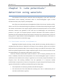
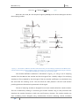
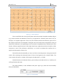
One aspect to be taken under consideration is the phase distortion induced by the filter. In
non-stationary signals this distortion may lead to significant errors. Another factor to always take in
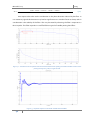
consideration is the stability of the filter. This may be tested by observing the filter’s response to a
Dirac impulse. This filter responds in a muffled fashion typical of a stable passing-band filter.
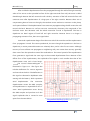
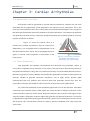
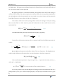
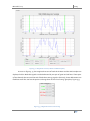
Figure 4.2 - Transfer function and phase of the fourth order Butterworth's passing-band filter. Marked red there is the
passing-band (40 to 250 Hz) on a gain of 0 dB.
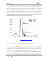
Figure 4.3 - Impulsive response to the fourth order Butterworth filter.
42
MicroECG v2.4
2009
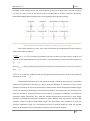
Another characteristic of this method is the calculation of a detection function defined by
the equation:
𝑉𝐴 =
𝑥(𝑡)2 + 𝑦(𝑡)2 + 𝑧(𝑡)2
(4.7)
Where x(t), y(t) and z(t) are the instantaneous amplitudes in all three derivations after
filtering and 𝑉𝐴 is the amplitude vector.
After peak detection the QRS should be delineated by its start and endpoints. The start of
the QRS complex is defined to be the start of the Q wave (or maybe even the R wave when Q is not
present). The endpoint of the QRS complex is defined to be the end of the S wave (or the end of the
R wave when S is not present).
The localization of the start and endpoints of the QRS complex is made through an
algorithm proposed by Simson. This algorithm applies to the 𝑉𝐴 curve. A sample of noise is
measured, then through a 5 milliseconds window is located the zones where the mean of 5
points are superior to the mean plus 3 times the standard deviation of the noise sample. The
mean point of the 5 millisecond segment is the last point that belongs to the QRS complex.
For the determination of the QRS start, the noise sample has 20 milliseconds and starts 50
milliseconds before the beginning of the QRS. For the determination of the QRS’s endpoint
the noise sample has 40 milliseconds and starts 60 milliseconds after the end of the QRS
(the window runs on the opposite direction for this case).
4.2 Magnitude vector’s parameters
There are three parameters derived from the filtered vector magnitude. The first is the QRS
duration, which is often abbreviated in the literature as QRSd. The QRS duration is the difference
between the end and the start of the QRS.
𝑄𝑅𝑆𝑑 = 𝑄𝑅𝑆𝑜𝑓𝑓𝑠𝑒𝑡 − 𝑄𝑅𝑆𝑜𝑛𝑠𝑒𝑡
(4.8)
The QRSd is a measure of total ventricular activation time, that is, it measures the time from
the earliest ventricular activation to the time of latest ventricular activation. In the high-resolution
mode, this applies to the termination of the low-level late potentials. The value of QRSd considered
to be abnormal is variable among a number of studies depending on the study objectives. Abnormal
QRSd values range from 110 to 120 milliseconds, with the most common value being 120
milliseconds.
43
MicroECG v2.4
2009
The other two late potential parameters also rely primarily on the 𝑄𝑅𝑆𝑜𝑓𝑓𝑠𝑒𝑡 point. They are
the root mean square (RMS) voltage and the low-amplitude signal (LAS) duration. Both are obtained
from the filtered vector magnitude. They measure features of the late potential waveforms and do
not directly relate to the electrophysiology of the heart as the QRS duration does. From these
waveforms, several parameters have been derived such as total QRS duration (including late
potentials), the RMS voltage value of the terminal 40 ms (RMS40), and the low-amplitude signal
(LAS) duration from the 40-μV level to the end of the late potentials. Abnormal values for these
parameters are used to identify patients at high risk of ventricular tachycardia following a heart
attack. Essentially, a late potential appears as a low-level “tail” after the main body of the QRS
complex. The RMS and LAS are designed to be descriptors of this late potential tail. The threshold
for an abnormal value of RMS40 is most commonly less than or equal to 20 milliVolts and for the
LAS, values greater than or equal to 20 milliseconds are considered abnormal. [Brecker 1992]
After a number of studies involving the three Simson’s parameters the “American College of
Cardiology” published a document with the objective to set standard values to these parameters.
So, following this document, the appearance of late potentials, assuming the use of a bidirectional
Butterworth filter with a passing-band of 40 to 250 Hz, includes a:

QRSd of 114 milliseconds.

RMS40 inferior to 20 microvolts.

LAS40 superior to 38 milliseconds.
However, the existence of these values is known for the QRS complex, there are none
available information through the Simson’s studies to the RMS values on P-Wave or even its
duration. So, this interface should be used as a platform for future studies in this area.
The limits of this method are related with the quality of the HR-ECG signal. The level of
noise, for instance, is one difficult parameter to measure, depending on the location of the
measurement window. The QRS endpoint location, is one measurement that strongly influents the
other three parameters’ values. Another limitation to the Simson’s method is the fact that only
detects late potentials located on the end of the QRS complex or in the ST segment.
44
MicroECG v2.4
2009
Chapter 5: Late potentials’
detection using wavelets
The utilization of time-frequency methods in electrocardiography is quite useful. This kind of
representation allows obtaining information about an electrocardiographic signal in three
simultaneous levels; time, frequency and amplitude.
One of the most used techniques is the application of Short-Term Fourier Transform (STFT),
where a set of FFT are calculated through the application of windows that overlap along the signal.
The location and duration of this signal’s segment defines the temporal precision of the spectral
estimative. However, the application of the STFT has his disadvantages. His time-frequency
precision is not great. The temporal precision could be enhanced if the window’s duration is
diminished, but this would also diminish the frequency resolution. Due to this limitation, STFT’s are
losing ground in high-resolution electrocardiography to wavelet transformations, also known as
time-scale representations. [Gramatikov 1995]
5.1 Continuous wavelet transformation
Regarding biomedical signal processing, namely HR‐ECG processing, Wavelet analysis is
considered the state‐of‐the‐art method for the analysis of non‐stationary signals such as the ECG
itself and the micro-potentials inside. Fourier analysis is simply not suitable for the analysis of short
lived low amplitude signals buried in higher amplitude signals. Thus the crescent interests in this
new methodology for non‐stationary signal analysis. [Frénay 2009]
Continuous wavelet transformation (CWT) is based on a set of analyzing wavelets (from the
French “ondelette”) that allow the decomposition of an electrocardiographic signal in a series of
coefficients. Each wavelet used to analyze a signal has its own duration, temporal localization and
frequency band. The resulting coefficient from the application of a continuous wavelet
transformation corresponds to a measure of components, on a given temporal and frequency band,
segment of the HR-ECG. A coefficient is obtained through two major steps:
1. The multiplication of a analyzing wavelets and a HR-ECG segment.
2. The measurements of the area bellow the resulting curve. From a mathematical point of
view this transformation is given by:
45
MicroECG v2.4
2009
𝐶(𝑎, 𝑏) =
1
𝑎
𝐸𝐶𝐺 𝑡 𝛹
𝑡−𝑏
𝑎
. 𝑑𝑡
(5.1)
Where a is the scale, b is the temporal segment, ECG (t) is the electrocardiogram and Ψ is
the analyzing wavelet.
Figure 5.1 - The wavelet-coefficient calculation is illustrated using a set of analyzing wavelet from the ‘Mexican hat’
wavelet and the ECG signal from a healthy subject. Extracted from “Contribution of the Wavelet Analysis to the NonEvasive Electrocardiology”, Couderc, pg. 56. [Couderc 1998]
The wavelet-coefficient calculation is illustrated in figure 5.1 is using a set of analyzing
wavelet from the ‘Mexican hat’ wavelet and the ECG signal from a healthy subject. The analyzing
wavelets are first multiplied by the ECG signal. Then the wavelet coefficients are calculated using
the area under the resulting curves. The area values are then plotted in the time-scale domain
providing the three-dimensional representation of the signal.
The set of analyzing wavelets is designed from a basic wavelet called the ‘mother wavelet'.
This set is obtained by dilating or contracting the mother wavelet using a scale parameter that
describes the wavelet dimension in both time and frequency domains. The mother wavelets are
short oscillating waves designed using mathematical functions satisfying several conditions
46
MicroECG v2.4
2009
including a mean value equal to zero and boundaries quickly converging to zero. As seen on figure
5.2 there are many kinds of wavelet functions including Morlet wavelet, Gaussian derivatives,
Daubechies, Mallat, Meyer wavelets that can be applied to ECG signal processing.
Figure 5.2 - Frequently used wavelet functions in ECG signal processing. Extracted from “Contribution of the Wavelet
Analysis to the Non-Evasive Electrocardiology”, Couderc, pg. 58. [Couderc 1998]
The mother wavelet is a wave, that, when represented by mathematical functions have to
satisfy three major conditions:
𝛹(𝑤) 2
. 𝑑𝑤
𝑤
< +∞ This condition guarantees that the wavelet could be used to analyze and
reconstruct the signal without lost of information. Ψ (w) represents the Fourier Transformation of Ψ
(t).
(5.2)
|𝛹(𝑤)|2
zero.
𝑤=0
= 0 This condition guarantees that the Fourier Transformation is null for w equal to
(5.3)
𝛹 𝑡 . 𝑑𝑡 = 0 This last condition is the one that guarantees that the mean value of the wavelet in
time domain is null.
(5.4)
The wavelet is located in time using a time parameter. Therefore this technique is also called
time-scale transformation. The figure 5.3 shows how the dilatation or contraction of the mother
wavelet has influence on the time and frequency characteristics. When the wavelet is dilated (longer
in time), its frequency bandwidth is narrowed and centered in low frequencies. On the other hand,
when the wavelet is contracted (shorter time duration), its frequency bandwidth is widened and
centered in higher frequencies. Thus, when the wavelet analyzes slow waves as the T wave, longer
wavelets are needed and frequency resolution is good. Whereas with rapid waves, like the QRS
complex, shorter wavelets provide better signal time description: time-resolution is good but
frequency resolution is poor. As a microscope can focus on specific details of a slide, the wavelet
shape can be adapted to focus the analysis on specific components of the ECG.
47
MicroECG v2.4
2009
Figure 5.3 - An example of a set of analyzing wavelets from the 2nd Gaussian derivative ('Mexican Hat') is plotted. The
wavelets are represented in both the time (left panel) and the frequency (right panel) domain. The mother wavelet is
drawn with a bold line in the time and frequency domains. Extracted from “Contribution of the Wavelet
Analysis to the Non-Evasive Electrocardiology”, Couderc, pg. 59. [Couderc 1998]
Each wavelet has for every scale a frequency band, in a way that can’t be associated a scale
to a given frequency. However there is a relation between the central frequency of a wavelet and its
scale. This relation is given by: 𝐹𝑎 =
𝛥𝐹𝐶
𝑎
(5.5),
where a is the scale, Fc is the wavelet’s central
frequency and Δ is the sampling period of the transformation signal.
Because the efficiency of the time-domain late-potential detection is limited to the terminal
portion of the QRS complex and is also affected by inaccuracies of QRS-end detection, frequencydomain methods have been investigated.
The HR-ECG analysis is the field of research most actively seeking to benefit from the
wavelet signal-processing technique. In 1989, Meste [Meste 1989] applied for the first time, the
wavelet transform to 5 KHz sampled ECGs. Subsequently, they used the Meyer wavelet for the
detection of the late potentials. The first quantitative analysis of the HR-ECG using wavelet
transformation was described by Dickhaus, who identified significant differences in HR-ECG
between post-infarction patients with ventricular tachycardia and healthy subjects.
A different approach was used by Shinnar and Simson [Shinnar 1992] who examined the
local scaling behavior of the ECG wavelet transformation. Patients without ventricular tachycardia
produced ECG wavelet transformation with relatively constant slope, while patients prone to
ventricular tachycardia produced ECG wavelet transformation with variant behavior. Couderc
[Couderc 1996] and Rubel [Rubel 1995] reported studies using non-redundant waveletdecomposition of the HR-ECG for the accurate description of the time-frequency components of
late potentials without the need of QRS-endpoint localization. In populations of post-myocardial
infarction patients with and without sustained ventricular tachycardia, new quantifiers quantifying
the energy of the high-frequency components (125-250Hz) from the QRS-ST complex were defined.
These new parameters had higher discriminative power than the time-domain parameters. More
48
MicroECG v2.4
2009
recently, Reinhardt [Reinhardt 1996] and Sierra [Sierra 1996] from the same group published two
wavelet-based approaches for HR-ECG analysis. Reinhardt studied the value of a wavelet correlation
function providing a type of spectral turbulence or scale turbulence quantification. The authors
reported more spectral changes in the QRS complex of anterior myocardial infarction than in inferior
myocardial infarction. Moreover the combination of time-domain analysis of late potentials and
wavelet correlation functions increased the prognostic value of the ECG for predicting cardiac
events after myocardial infarction.
MicroECG software package also offers the user the possibility to deeply analyze the HRECG in a wavelet-based approach. Figures 5.4, 5.5 and 5.6 are an example extracted from the
software itself that show the MicroECG’s capabilities to construct a time vs. frequencies scalogram
using different detection wavelets.
Figure 5.4 – MicroECG obtained scalogram for the P-wave using the detection wavelet: cgau4
49
MicroECG v2.4
2009
Figure 5.5 – MicroECG obtained scalogram for the P-wave using the detection wavelet: db2
Figure 5.6 – MicroECG obtained scalogram for the P-wave using the detection wavelet: fb33sp1-1-1
50
MicroECG v2.4
2009
5.2 Discrete wavelet transformation and wavelet packets
Calculating wavelet coefficients at every possible scale is a fair amount of work, and it
generates an awful lot of data. Can it be chosen only a subset of scales and positions at which to
make the calculations?
It is known now that, if it is chosen a scales and positions based on powers of two — socalled dyadic scales and positions — then our analysis will be much more efficient and just as
accurate. This is known as the discrete wavelet transformation (DWT).
For many signals, the low-frequency content is the most important part. It is what gives the
signal its identity. The high-frequency content, on the other hand, imparts flavor or nuance.
Consider the human voice. Removing the high-frequency components, the voice sounds different,
but can still be told what’s being said. However, if removed enough of the low-frequency
components, gibberish is heard.
In wavelet analysis, we often speak of approximations and details. The approximations are
the high-scale, low-frequency components of the signal. The details are the low-scale, highfrequency components, so the filtering process, at its most basic level, looks like figure 5.7.
Figure 5.7 – The original signal S, passes through two complementary filters and emerges as two signals.
These signals A and D are interesting, but we get twice as many values instead of the length
of the original signal. There exists a more subtle way to perform the decomposition using wavelets.
By looking carefully at the computation, we may keep only one point out of two in each of the
samples to get the complete information. This is the notion of downsampling. As seen on figure 5.8,
on the left, we produce two sequences called cA and cD.
Figure 5.8 – The process on the right, which includes downsampling, produces DWT coefficients.
51
MicroECG v2.4
2009
The decomposition process can be iterated, with successive approximations being
decomposed in turn, so that one signal is broken down into many lower resolution components. This
is called the wavelet decomposition tree. This notion can be better visualized on figure 5.9, as it
shows the frequencies intervals used by each sub-signal.
Figure 5.9 – Wavelet decomposition tree.
Since the analysis process is iterative, in theory it can be continued indefinitely. In reality,
the decomposition can proceed only until the individual details consist of a single sample or pixel.
In the wavelet packet framework, compression and de-noising ideas are exactly the same as
those developed in the wavelet framework. But as it can be visualized by figure 5.10, the main
difference is that wavelet packets offer a more complex and flexible analysis, because in wavelet
packet analysis, the details as well as the approximations are split.
Figure 5.10 - Wavelet packet decomposition. Adapted from
http://www.mathworks.com/access/helpdesk/help/toolbox/wavelet/index.html?/access/helpdesk/help/toolbox/wave
let/ch05_us2.html
One single wavelet packet decomposition “tree” gives many bases from which one can look
for the best representation with respect to a design objective. This can be done by finding the "best
tree" based on an entropy criterion. The difference between discrete wavelet transformation and
wavelet packets is that wavelet packet present all the same frequency resolution in all the nodes in
the same level, since the signal’s approximation and detail nodes are all split into two new signals,
52
MicroECG v2.4
2009
instead of only the approximation node being split as it happens in the discrete wavelet
transformation process, because of this the wavelet packets turn out to be more efficient to study
high resolution cases because there are no significant loss of detail in higher frequencies. Another
important thing to take notice is that the final level of this multi-level decomposition “tree” are the
coefficients that can be used to reconstruct the original signal. However these coefficients or
“leaves” of this “tree” are in no sequential order in terms of frequency, and one most take notice of
this fact if it wants to reconstruct the signal from this coefficients. Finally, a final note to the number
of iterations or levels calculated in MicroECG. These levels are calculated via the length of the signal
and its frequency sampling. The “leaves” of this wavelet packet decomposition “tree” is always a
power of 2, for example, if a number of 8 levels are calculated there will be 256 “leaves” or
coefficients in the end. However, all these 256 “leaves” are shown if the user selects all frequencies
to be analyzed from zero to half the used frequency sampling. If the user only selects an eighth or a
quarter of the frequencies available to be analyzed therefore these 256 “leaves” are cut also by an
eighth and a quarter. For better exemplify these same principles, figures 5.11 and 5.12 are shown. In
both figures the red line corresponds to the reconstructed signal and the blue line the original signal.
In page 106 of this thesis there is a better explanation of this figure.
Figure 5.11 – DWT reconstruction and respective values for the coefficients found for an eighth of the available
frequency band width. Only 32 of possible 256 coefficients are shown. The reconstruction of the signal, using all the
found coefficients, when compared with the original signal suffers some degradation.
53
MicroECG v2.4
2009
Figure 5.12 – DWT reconstruction and respective values for the coefficients found for a quarter of the available
frequency band width. Only 64 of possible 256 coefficients are shown. The reconstruction of the signal, using all the
found coefficients, when compared with the original signal suffers less degradation than the previous example.
54
MicroECG v2.4
2009
Chapter 6: ActiveTwo System
The ActiveTwo system was designed for multi channel, high resolution biopotential
measurement systems for research applications. The system is a further development of the
previous ActiveOne system, the first commercially available system with active electrodes.
Advances in technology have allowed to significantly increasing the number of channels, digital
resolution, input range, and sample rate, without any increase in size, power-consumption or costs.
Second generation active electrodes are smaller in size with less cable weight, while offering even
better specs in terms of low-frequency noise and input impedance. The new ActiveTwo system and
its components, figure 6.1, features:

Head cap system with the fastest application time.

Reliable measurements without skin preparation.

Battery powered front-end with fiber optic data transfer.

Suitable for EEG, ECG as well as EMG measurements.

Graphical programming (LabVIEW) on PC and Mac.

Full range of auxiliary sensors available.

MEG/MCG compatible digital system.

Up to 256+8 electrode + 7 sensor channels in a single ultra compact box.

Second generation active electrode: smaller size & less weight.

Flexible colored electrode labeling system.

24 bit ADC per channel, unsurpassed signal/noise ratio and linearity.

Improved digital resolution, LSB value is 31nV.

Full DC operation, largest input range in the industry (524mVpp).

User selectable sample-rate 2, 4, 8, 16 kHz/channel.
Active Electrodes & Headcaps
Fiber
Charger
Battery Box
PC-Laptop
USB2 Receiver
AD-Box
Software / ActiView
USB2
Analog Input Box
Figure 6.1 - ActiveTwo System and its components.
55
MicroECG v2.4
2009
6.1 Components
Active Electrodes
By integrating the first amplifier stage with a sintered Ag-AgCl
electrode, extremely low-noise measurements free of interference are
now possible without any skin preparation. The Active-electrode is a
sensor with very low output impedance, all problems with regards to
capacitive coupling between the cable and sources of interference, as
well as any artifacts by cable and connector movements are completely
eliminated. Noise levels as low as the thermal noise level of the electrode
Figure 6.2 - Flat-type activeelectrodes. Extracted from
http://www.biosemi.com/acti
ve_electrode.htm
impedance (which is the theoretical minimum) is achieved.
The electrode, figure 6.2, is completely resistant to water and alcohol. These electrodes
have an input protection circuit that protects the electronic amplifier from static discharge and
defibrillator pulses. The use of sintered Ag-AgCl electrode material ensures low noise minimal offset
potentials and excellent DC-stability (low drift,) without the need for any re-chloration; all versions
of the Active electrodes are suitable for low-drift DC measurements. The smart electrical and
mechanical design allows to produce the active electrodes at the same costs (EUR 30, - per
electrode) as conventional high quality electrodes. Significant savings on operational costs can be
achieved because of the reduced application time, the high reliability of the measurements and the
elimination of the re-chlorisation tasks. BioSemi offers Active-electrodes in several versions to adapt
to the various needs in the EEG, ECG and EMG field; still, for this study the Flat-type activeelectrode was the choice, so here are their main characteristics:
56

Suitable for all Body-surface applications: EEG, ECG, EMG.

Easily attached to the skin with electrode paste or adhesive disks.

Gel cavity reduces motion artifact and gel dry-out.

32 electrodes on a common connector.

140 centimeter cable length, other lengths on request.
MicroECG v2.4
2009
AD-Box
The ActiveTwo AD-box, figure 6.3, forms an ultra compact, low
power galvanically isolated front-end (close to the subject) in which up to
256 sensor-signals are digitized with 24 bit resolution. These sensors can
be active electrodes but also BioSemi buffer boxes with normal passive
electrodes, as well as a range of additional active sensors measuring
parameters like respiration, temperature, force etc. Each AD-box channel
consists of a low noise DC coupled post-amplifier, with a first order antialiasing filter, followed by a Delta-Sigma modulator with an
oversampling rate of 64, and decimation filter with a steep fifth order
Figure 6.3 - Analog/Digital
Box. Extracted from
http://www.biosemi.com/adbox_activetwo.htm
synchronized response and high resolution 24-bit output. The digital outputs of all the AD
converters (up to 256) are digitally multiplexed and sent to the PC via a single optical fiber without
any compression or other form of data reduction. This is the AD-box main characteristics:

Special input stage matched with the output of the new 2-wire Active electrodes.

Power supply to active electrodes has auto-shutdown for optimal safety.

ADC per channel offers synchronized sampling, no skew and zero-reference principle.

24 bit sampling, 31nV digital resolution with guaranteed no missing codes.

Sigma-Delta converter technology for unsurpassed linearity and dynamic range.

Configurable/upgradeable number of channels: 8 up to 256 channels.

Up to 16 kHz sample-rate per channel, user selectable (1.5MByte/sec total throughput).

Full DC operation, with input range as large as found in AC designs.

Battery power supply with fiber optic link offers optimal interference rejection and subject
safety.

Low power design: 5 hour battery life for 256 channels, 1 week for 8 channels.
USB2 Receiver
The Receiver, figure 6.4, converts the optical data coming from
the AD-box to an USB2 output. In addition, the USB2 receiver has a
trigger port with 16 independent trigger inputs and 16 independent
trigger outputs. This setup keeps the complete stimulation setup
galvanically isolated from the subject. The trigger output signals can be
controlled with an extra independent LabVIEW thread integrated in
Figure 6.4 - USB2 receiver.
Extracted from
http://www.biosemi.com/receiv
er.htm
57
MicroECG v2.4
2009
the BioSemi acquisition software. The trigger inputs allow easy setup of EP/ERP measurements, and
event logging.
The New USB2 Receiver offers extremely setup and installation (Plug and Play) combined
with fully reliable high speed data throughput. A 256 channel 24bit ActiveTwo system at 4096 kHz
including a 32 channel Analog Input Box at 4096 kHz has a total data throughput of 3.54MByte/sec.
The ActiView acquisition software streams this data reliable to disk.
The USB2 receiver allows the ActiveTwo system to be used with both desktops and
notebooks. With the notebook option, you can realize a completely portable (everything fits in a
small bag, less then 4Kg including notebook) 256 channel EEG/ECG/EMG system, independent of
the mains supply. So, here’s a resume of this components main characteristics:

USB2 standard interface

Large (4Mbit) internal buffer for guaranteed Gap-Free data streaming to the PC.

Fully powered though the USB2 port. (no extra adapter needed)

37 pins Sub-D connector at the back provides 16 input and 16 output triggers.

Trigger inputs remain galvanically isolated from AD-box, electrodes and subject.

LED indicator for indication of data coming from the fiber.

LED indicator for indication of data communication with USB2 port.
Laptop
Standard personal computers are used with BioSemi systems. BioSemi systems can be
delivered with or without a PC/Laptop. The BioSemi USB2 interface features a very low CPU usage,
which gives the user the possibility to do data acquisition even with low-cost PC's.
Software
All Biosemi’s systems are delivered with acquisition software
based on the LabVIEW graphical programming language from National
Instruments seen on figure 6.5. This standard package handles the
basic functions like data acquisition, display on screen with all usual
scaling and reference and filtering options, streaming to disk in .BDF
file format and network sharing. Thanks to the flexible setup of
LabVIEW, it is easy to modify the standard program for specific
applications. This way can be obtained a virtually "custom made"
acquisition program.
58
Figure 6.5 - ActiView software.
Extracted from
http://www.biosemi.com/softwa
re.htm
MicroECG v2.4
2009
Charger
A separate charger, figure 6.6, is supplied with the system to
allow quick charging of the battery when used in cyclic applications.
The special sealed lead-acid batteries that are used in the battery-box
can be charged very quickly with the specially designed charging
circuit: full charging of an empty battery takes about 3½ hours. The
charger automatically switches to a float state when the battery is fully Figure 6.6 – Charger. Extracted
charged, and the battery can be left on the charger for unlimited time
without any reduction of the operation life. A battery life of approx.
from
http://www.biosemi.com/char
ger.htm
1000 recharge cycles can be expected.
Battery Box
The battery-box, figure 6.7, is the power supply of the AD-box
and Active electrodes. The battery-box contains a sealed lead-acid
battery and a shutdown circuit to prevent the battery from deep
discharge. The combination of a large capacity battery and very low
power consumption of the AD-box and Active electrodes makes the
ActiveTwo the only real battery powered, high number of channel
system. In 256 channel version battery life is at least 5 hours, less
channels offer extended battery life, up to 3 days for a 16 channel
Figure 6.7 - Battery box.
Extracted from
http://www.biosemi.com/batter
y_box.htm
version. Given the charge time of less than 4 hours, continuous longtime measurements are possible
with the 2 standard provided batteries. (Battery can be changed in less than 10 seconds. Double
capacity batteries are available for users needing double battery live. Optionally, the BioSemi
acquisition software can detect whether a battery is replaced by another battery. When the second
battery is connected to the amplifier within 30 seconds, the acquisition will resume normally. This is
the battery box main characteristics:

Large capacitance, compact battery.

No memory effect, batteries can be recharged in any state of charge.

More than 10 hours continuous operation time for 128 channel system.

Shelf life of charged batteries is at least 6 months.

Power box can be quickly replaced.

Long life, at least 1000 charge/discharge cycles.

Automatic shutdown when battery is empty to prolong battery life.
59
MicroECG v2.4
2009
Analog Input Box
The standard ActiveTwo AD-box, figure 6.8, measures signals
from electrodes or other sensors connected to the subject. But in
some measurements setup, one also needs to measure additional
analog signals from sources that needs to be kept isolated from the
subject (for example because the sources are mains powered
equipment). For these applications, BioSemi offers a sophisticated
solution in the form of an extra Analog Input Box (AIB). The subject
Figure 6.8 - Analog Input Box.
Extracted from
http://www.biosemi.com/aib.htm
AD-box and the AIB are daisy chained by optical fibers: a fiber-optic
data link goes from the subject AD-box to the AIB, and a second optical fiber goes from the AIB to
the receiver which is located in the PC. The AIB adjusts its sample rate to the signal received from
the subject AD-box, so the sample rates of both boxes are synchronized. The subject AD-box
acquires up to 256 channels from electrodes and other sensors, the AIB adds up to 32 channels to
the data stream, and the total of 288 channels is processed by the PC. This setup allows all the 288
channels (from different sources) to be handled by one integrated software program, and to be
stored in a single BDF file. Standard, the AIB is equipped with 8 channels (4 differentials). This is the
Analog Input Box main characteristics:

Universal high impedance inputs with static protection.

Powered by mains or by battery.

Input range: +/-260mV or +/-1Volt on request.

ADC per channel offers synchronized sampling, no skew.

24 bit sampling, with guaranteed no missing codes.

Sigma-Delta converter technology for unsurpassed linearity and dynamic range.

2 kHz sample-rate per channel fully synchronized with subject AD-box.

Full DC operation, with input range as large as found in AC designs.

Fiber optic link offers optimal interference rejection and subject safety.
60
MicroECG v2.4
2009
6.2 Technical specifications
Sample-rate options: (sample rate is adjustable by
user)
2048 Hz
4096 Hz
8192 Hz
16,384 Hz
Max. number of channels @ selected sample rate:
280
152
88
56
DC - 400 Hz
DC - 800 Hz
DC - 1600 Hz
DC - 3200 Hz
Bandwidth (-3dB):
th
Low-pass response
5 order sinc digital filter
High-pass response
Digitalization:
fully DC coupled
th
24 bit, 4 order Delta-Sigma modulator with 64x oversampling,
one converter per channel
Sampling skew:
Absolute sample rate accuracy (over temp range: 070 C)
< 10 ps
0.1 Hz
0.2 Hz
Relative sample rate accuracy (jitter)
Quantization-resolution
0.4 Hz
< 200 ps
LSB = 31.25 nV, guaranteed no missing codes
Gain accuracy:
Anti aliasing filter
Total input noise (Ze < 10 kOhm):, full bandwidth
1%
fixed first order analog filter, -3dB at 3.6 kHz
0.8 uVRMS
(5 uVpk-pk)
1.0 uVRMS
(6 uVpk-pk)
1.4 uVRMS
(8 uVpk-pk)
1/f noise (Ze < 1 MOhm):
1 uVpk-pk @ 0.1..10Hz
Amplifier current noise:
< 30 fArms
Input bias current:
Input impedance Active Electrode
DC offset:
DC drift
Input range
Distortion
Channel separation
12
300 MOhm @ 50 Hz (10 Ohm // 11 pF)
< 0.5 mV
< 0.5 uV per degree Celsius
+262 mV to -262 mV
< 0.1 %
> 100 dB
> 100 dB @ 50 Hz
Isolation Mode Rejection Ratio
> 160 dB @ 50 Hz
Battery capacity, standard battery
Battery life on standard battery
Battery charge time (with external fast charger):
4 Watt @ 280 channels
inversely proportional with the number of installed channels
25 Watt-hour, 3 cell sealed lead-acid
(double capacity battery is available as an option)
> 5 hours @ 280 channels
inversely proportional with the number of installed channels
< 3.5 hours for a 100% charge
Leakage current, normal operation:
< 1 uA rms.
Leakage current, single fault
< 50 uArms
Trigger inputs:
Trigger outputs:
PC interface:
Size of front-end, including battery-box (H x W x D)
2.0 uVRMS
(12 uVpk-pk)
< 100 pA per channel
Common Mode Rejection Ratio
Power Consumption
0.8 Hz
16 inputs on optical receiver (isolated from subject section) , TTL
level
16 outputs on optical receiver (isolated from subject section) , TTL
level
USB2.0
120 x 150 x 190 mm
Weight of front-end, including battery-box
1.1 kg
Warranty
3 years
61
MicroECG v2.4
2009
Chapter 7: Data acquisition
The most recent data acquisition was done using Biosemi’s ActiveTwo system. This system
offers the possibility to easily record HR-ECG signals with minor preparations and some comfort.
However, even if the system is easily set up and comfortable for the subject, some minor
preparations are always needed. Skin preparation is vital when placing the electrodes. The body
surface/electrode interface must be cleaned but the usual sand-paper skin preparation is not
required for this system, so in order to achieve low noise, minimal offset potential and DC stability
(low drift), the use of alcohol or water prior to the positioning of the electrodes is advised. For extra
body surface/electrode contact the ActiveTwo system comes with some electrode gel and adhesive
disks to ensure that once the electrodes are in place they won’t move and disturb the data
acquisition.
The electrode positioning is also an important factor in acquiring the HR-ECG data. The
selection of the electrode positioning was made to ensure that the signal quality is enough for a
robust P-wave, since this is the lowest amplitude signal on the ECG.
Figure 7.1 - Electrode positions used during the HR-ECG data acquisition (Frank’s leads).
62
MicroECG v2.4
2009
Figure 7.1 shows the electrode position used during the HR-ECG data acquisition, this
positioning was based in the Frank’s studies to obtain an orthogonal representation system in three
dimensions. The CMS stands for Common Mode Sense, and DRL is Driven Right Leg.
Ventricle Level: For ordinary clinical routine use the transverse level of the ventricles may be
taken as the fifth interspace (at the sternum). Some error may be introduced using this level, but it is
usually within 1 inch of the correct level. Electrodes 1, 2, 3, 4 and 5 are all located at precisely the
same anatomic level. When the subject is capable of standing, the level may be marked around the
chest by the use of a string with a weight on the end (plumb bob) adjusted in length so that the
weight just touches the floor at various points around the steady subject.
Angular Locations of Chest Electrodes: Electrodes 3 and 5 are placed exactly on the front and
back midlines, respectively. Electrodes 1 and 4 are placed on the left and right midaxillary lines,
respectively. The meaning of midaxillary line, as used here, is a line passing exactly through the
axilla and parallel to the central axis of the trunk. The vertical plane containing 1 and 4 is typically
closer to the back than to the precordium, often cutting the thorax in the ratio 1.2:1. Various types of
chest protractors may be devised that permit the location of electrode 2 to be established at an
angle of 45 degrees between electrodes 3 and 1. This location is often deceptive because of
precordial contour, and anatomic distances on the body surface from 1 to 2 and from 2 to 3 are
usually unequal.
Head and Foot Electrodes: Electrode 6 is placed on the back of the neck 1 cm. to the right of
the back midline at a level corresponding to the extension of the top shoulder line across the back.
Its location is not especially critical. Electrode 7, least critical of all, its standard location is on the left
leg, between the knee and ankle.
In female subjects, electrode 2 has some unavoidable error when the transverse level of the
ventricles does not fall above or below the left breast. This error is not acute because electrode 2
serves as a correction for Vx, is weighted by about 27 per cent in its contribution to the three resistor
junction of Vz, and does not affect Vy, at all.
Contrary to the advice given by Frank, [Frank 1956] in relation to the subject’s posture when
performing the data acquisition, it was found to be more relaxing to the subjects to be lay down on a
bed and carefully covered by a blanket, instead of a sitting position, since this way it was found to
induce less muscle tremor and therefore less noise due to muscular activity.
63
MicroECG v2.4
2009
Chapter 8: Algorithms
all the major functionalities of
Wavelets
Fine Tunning
Figure 8.1 diagram shows
the MicroECG software package.
As can be seen there are two
ways of loading data into the
software; via the simulator or via
a .bdf or .mat file data. After the
MicroECG’s General Process Diagram
this data will be analyzed to find
Magnitude
Vectors
Show Template
software reads the HR-ECG data,
the peak points (R points) of an
electrocardiographic signal. As
12-Lead ECG
this peak points are found, they
are selected and aligned to
construct a template through
Raw Data From
Electrodes
Peak Detect
Read File
Open File
signal averaging. After this point,
the software allows the user the
most of its capabilities like ECG
Variability, Heart Rate Variation,
Noise Level
Between Heart
Beats
measurement of the noise level,
display of the raw data acquired
and display of a 12 lead HR-ECG,
measurement of the magnitude
Heart Variation
Rate
vectors’ parameters or even use
the wavelet package. One thing
to notice is that as the template
ECG Variability
Late Potential
Simulator
construction automatically finds
and delineates the various parts
of a heartbeat like the P-Wave,
QRS complex and the T-Wave the
medical
user
also
as
the
opportunity to fine tune these
Figure 8.1 –MicroECG’s general process diagram
64
delineations (this is especially
MicroECG v2.4
2009
useful when using the wavelet package). The use of these fine tuning buttons on the measurement
of the magnitude vectors’ parameters will also allow the user to see how the parameters change
accordingly to the delineations imposed.
Late Potential Simulator
Figure 8.2 shows how the late potential
simulator was implemented to work the MicroECG’s
The user is asked to enter some
parameters to induce a late
potential on a short and
algorithms when in the absence of real acquired high
simulated ECG example.
Parameters include Amplitude,
Width, Position, Cut-Off
previously this part of the software evolved so that
Frequency, and Noise Level.
absence of human test subjects that suffered from the
resolution electrocardiographic signals. But as stated
could be used as a late potential generator when in the
late potential artifacts.
This parameters will modify the
simulated ECG and induce an
artifact following this same
choose or insert a few initial late potential parameters
parameters.
to the software, so that the simulation on a small HR-
These simulator works by allowing the user to
ECG trench could occur. Some of these parameters are:
This obtained signal will
pass through a Frank matrix
of equations to correctly
display the simulated signal
in all X, Y, and Z vectors.
Amplitude – which indicates the late potential
amplitude in microvolts. This parameter usually is very
low and it is fairly normal to be somewhere around 10
or 20 microvolts. Width – indicates the time extension,
in milliseconds, which the late potential is expressed on
All projections of the simulated
signal are displayed to the
user the same way if the data
was obtained through a file.
the signal. The default value is set to 40. Position – the
position parameters is what will indicate in which part
of the template the late potential will occur. Note that
this position is relative to the middle of the QRS
All the same
procedures
mentioned above are
still valid to the
simulated signal.
complex, where theoretically the R point should be
present. The default value is set to 50 milliseconds,
where should generate a late potential in the end of the
QRS complex. However if the user wants to generate a
late potential on the P-wave a value of -140
Figure 8.2 – Late potential simulator diagram
milliseconds would be a good choice. The cut-off
frequencies are the frequency delineators in which the late potential will be expressed. These two
parameters will be entering in a pass-band filter which will actuate on the late potential artifact to be
inserted in the signal. This way the late potential will not excessively exceed the frequency
delimitations given by the user. Noise level – this input parameter is a value which will indicates the
65
MicroECG v2.4
2009
amplitude of the white-noise generated. This noise will be added to a core HR-ECG signal. This is an
important parameter if the user wants to simulate some muscular activity in order to create a more
realistic signal. [Berenfeld 1990]
After the simulated signal is generated with or without a late potential, seven version of this
signal are generated through the multiplication by different constant factors. These signals will pass
through the Frank’s system of equations so that the Frank’s derivations signals are obtained. Then
the peak detection will occur for signal averaging to take place, and the construction of a template
heart beat of this simulated signal can be achieved. After this point, all the major procedures of the
MicroECG will be available to the user, the same way that as if this simulated signal was obtained
through a data file.
Figure 8.3 diagram describes how the Open a
Open File
file will require the user to select a data file
Select a data file
.bdf file
.mat file
from either the recent recordings or the previous
recordings folders. This files are respectively
.bdf and .mat files. From either of these file
Extracts
personal
data from the
file header
using the
function
Extracts
personal
data from the
file header
using the
function
extractdata
conversor
types MicroECG software extracts the personal
and recording session information differently.
Personal and recording information such as
sample frequency, recording length, date,
subjects name, subject’s age, height, weight or
Figure 8.3 – Open file diagram
additional
information
are
detected
by
MicroECG from the file’s header. For the .bdf file types MicroECG uses the extractdata.m function to
read the file header and because these files are slightly different, since they were obtained through
different acquisition systems, they use different functions; the function to obtain the personal and
recording information from .mat files is named conversor.m. Note that, all information obtained in
these files is for research purposes only and could not be used for clinical treatment decisions.
66
MicroECG v2.4
2009
Read File
Figure
Read data file
8.4
diagram
show how after the opening of
the
Extract the
seven
electrodes
channels
file
personal
and
respective
and
recording
information obtained, the user
can choose just how much of
Detrend &
baseline mean
the recording session wants to
use. Because these recording
sessions are all around the 300
Seven2Frank
seconds mark (5minutes), it is
(Vx, Vy and Vz)
advised
to
use
all
the
information available, but still
Beat Detection
Co
nv
en
ci o
l
na
M
od
e
W
av
the user can choose the time
ele
interval that want to be
ts
M
nv
analyzed from the data file.
e
Then, MicroECG will finally
Detector_Carlos
QRSDetect
Co
od
en
ci o
na
lM
od
e
av
W
e
sM
let
od
commence
extracting
the
electrodes data and begin
e
with the signal processing.
Firstly, the seven electrode
Averaging all
beats,
construct
a temporary
template for X,
Y and Z
channels will be acquired and
for each one of them will be
made a signal channel detrend
to remove trends in the signal.
Given a correlation
constructs final
templates
for Vx, Vy and Vz
Get Heart Rate
Variation (HRV), mean
and standart deviation
A baseline mean extraction
will also take place. The seven
electrode channels will then
pass
Display Vx, Vy
and Vz in
seconds
Simson3
(outlines the P
wave, QRS
complex and Twave)
through
the
Frank’s
system of equations so that
the Vx, Vy and Vz vectors can
be obtained. By obtaining
these
three
Frank’s
derivations an automatic beat
detection method will now
Figure 8.4 – Read file diagram
67
MicroECG v2.4
2009
occur. This beat detection procedure will closely analyze each derivation by finding the R points of
each heart beat. In MicroECG there are two different methods for detecting heart beats. There is
what was called the conventional mode and there is the wavelet mode. The conventional and the
wavelet mode do exactly the same thing (finding heart beats) only in different ways with different
results. The conventional mode was a function developed by Schlögl in 2003 [Schlögl 2003], and it is
part of the BIOSIG Matlab toolbox. This algorithm works by finding the fiducial points of QRS
complexes and was firstly purposed by Afonso and Tompkins [Afonso 1999]. The wavelet mode uses
continuous wavelet transformations to detect the peak points of the Frank’s derivations. It was
developed in a previous version of this software tool and was based in the Sahambi’s work for the
ECG analysis through a wavelet approach [Sahambi 1998]. It has been our experience that the
wavelet detector produces better results in the presence of noisy recordings but is computationally
more demanding relatively to the Afonso and Tompkins classical detector.
After detecting these peaks points MicroECG will construct for each Frank’s derivation a
template beat of the found beats. By measuring all the R-R points’ time differences and by finding a
minimum value of these differences it can be set a time interval for the three templates. Then by
dividing these time difference in two it could be delimitated a beat, by setting from its R point minus
and plus these half time differences. If these same delimitations are used to delineate all the heart
beats, then all the isolated heart beats will be obtained with the same length. Then, by aligning all
the beats and averaging them, a temporary heart beat template is obtained. With these temporary
beats, the next step is use the user’s given correlation to select only the beats in each Frank’s
derivation that correlate with the temporary template to the user given correlation value. After this
selection a new and final template will be obtained, again through signal averaging. These
templates are the representative heart beat. Through signal averaging all the minor and sporadic
fluctuations of the cardiac signal are eliminated and all that’s left it is the systematic works of the
heart.
After achieving these heart beat templates MicroECG delineates from each one of them the
various parts (P-wave, QRS complex and T-wave) of the template. These delineations are obtained
through the method described by Sahambi’s work on ECG characterization. [Sahambi 1997]
Even if the construction of these templates is complete, the three Frank’s derivations display
should be the next logical step, so that the user can visualize the Vx, Vy, and Vz vectors and their peak
detection in green vertical lines.
68
MicroECG v2.4
2009
Aside from the construction of the template, the finding of the R-R points and their time
differences and calculation of its mean and sliding windows averages and standard deviations are
also useful to construct the Heart Rate Variation chart.
Bea
One
t Cor
relati
Automatic
Peak Detect
on
Wait for valid
double click one
heart beat
Outlines
Selected Beat
K Be
ge
Wait for valid
double click on k
heart beats
PicosDetect_v2
n
Co
v
c
en
i
on
M
al
od
e
W
av
el
et
s
Co
nv
M
od
Outlines
Selected
Beats
e
Detector_Carlos
QRSDetect
Given a
correlation
constructs
templates for
Vx, Vy and Vz
ats A
ve r a
en
ci o
na
lM
od
e
av
W
M
ts
ele
Averaging all
beats,
construct
a temporary
template for X,
Y and Z
od
e
Calculates the
mean for the
selected beats
and constructs
templates
Get Heart Rate
Variation (HRV), mean
and standart deviation
Given a correlation
constructs final
templates
for Vx, Vy and Vz
Oulines the P
wave, QRS
complex and the
T-wave
Figure 8.5 – Peak detection diagram
Figure 8.5 how MicroECG presents three different ways for the peak detection or heart
beats selection. The options are the Automatic, One Beat Correlation and K Beats Average modes.
The Automatic mode runs exactly as stated before in the Read File algorithm explanation. The other
two modes (One Beat Correlation and K Beats Average) could be seen as a variation of this Automatic
69
MicroECG v2.4
2009
mode. For the One Beat Correlation mode the user is asked to select, from the Vx, Vy and Vz display,
one single beat. This selection will skip a few steps when in comparison with the Automatic mode, as
this selected beat will serve as a temporary template to which all the remaining beats will be
correlated and furthermore selected for the construction of the final template. Note that, in all the
modes once after the algorithm achieves the final template, this same heart beat template is
delineated for every one of his parts (P-wave, QRS complex and T-wave). As for the K Beats Average
mode, this is quite simpler to explain, since the user is only asked to select the beats from the V x, Vy
or Vz display that it sees fit. Then these selected beats are aligned and signal averaging occurs with
these selected beats. The product of this averaging is already the final template and its constituting
parts are delineated for display.
Show Template
The show template procedure, figure 8.6, is very
simple too. The three template generated signals are set up
Displays templates in
miliseconds for
Vx, Vy and Vz derivations
and outlines the P wave,
QRS complex and T-wave
to be shown in milliseconds rather than in samples. Then,
since all the delineations are already calculated in the peak
detection algorithm these delineations are recalculated to fit
the signal in milliseconds as well.
Figure 8.6 – Show template diagram
The fine tuning procedure, figure 8.7, gives the
Fine Tuning
opportunity to the user by using a series of slider buttons to
fine tune the P-wave, QRS complex and T-wave’s limits
The user is given a
opportunity to fine tune the
outlines of the p wave, the
qrs complex or the T-wave
found by the software. There are two different situations
where the use of these buttons is important. The first
situation is in the accurate delineation of the various
constituting parts of the heart beat templates. The second
Figure 8.7 – Fine tuning diagram
situation is when in use of the magnitude vectors procedure,
because even if the MicroECG software attempts his best to delineate the start and end of the Pwave and QRS complex, these delineations may result inappropriate to medical user. Therefore as
the user fine tunes both the magnitude vectors start and end positions, MicroECG also recalculate
the parameters.
70
MicroECG v2.4
2009
The ECG Variability procedure, figure
ECG Variability
8.8, was first prompted by the Dr. Luis Brandão
Alves, in a visit to the Hospital Garcia de Orta.
The first idea was to study the variability to the
Choose part of the
template
T-wave alternans (TWA) [Jerneja 2009]. The
TWA itself detection was not performed in this
work. However it was the author decision to
P-Wave
QRS Complex
T-Wave
adapt these same principles to all the
constituting parts of the ECG templates, in all
of its leads and in all the detected beats or just
Choose Lead
the selected beats that constitute the ECG
template. This was made in order to maximize
MicroECG’s flexibility and potential. The
Y
X
Z
choosing of these three parameters are the
input to this ECG Variability procedure and
after this selection the procedure will take the
Select Beats
selected heart beats and align them vertically
so all of them begin at the same amplitude
Selected Beats
All Beats
offset position. The next step is to align them,
not vertically but horizontally by keeping these
Entering the parameters above, the
user has the opportunity, to perform
na ECG Variability check. This
procedure will begin by an vertical
alignment of all the desired beats .
beats closely behind each other and on the
same orthogonal plane. The representation of
this result in three dimensions is similar to a
river like effect where all the waves are spotted
The next step is to show a
tridimensional representation of all
the beats, all closely behind each
other and starting at the same
offset. This will create a river like
effect, with all the waves visible.
behind each other. These representations can
be further investigated by the user by using
some available tools that allow rotating,
zooming or scaling the heart beats in order to
Figure 8.8 – ECG variability diagram
extract more visual information about the
variability of the beats at hand. So an important fact to be taken account for is that, the direct result
of this representation is still very much a visual one, since there are no direct parameters calculated
in this procedure. It is the author’s opinion that it should be further work to be developed on this
matter, in future releases of this software package.
71
MicroECG v2.4
2009
The heart rate variation procedure, figure 8.9, is an
Heart Rate Variation
Calculates
Beat Differences
in Seconds
indirect result of the peak detection technique previously
explained. When in the peak detection the R-R distances were
calculated in order to calculate the maximum size for the heart
Calculates
Mean HRV
and STD
beat template, this same R-R distances could be used to calculate
all the consecutive beats differences. By converting these beat-tobeat distances to seconds and showing them to a chart, could help
Calculates
Mean through
sliding window
(Last 25 Beats
or less)
the MicroECG’s user to visualize the subject’s health state by
checking for abnormalities. The software will also display in this
chart the mean average of these beat-to-beat differences and its
standard deviation. There are two different zones in this chart that
Display HRV
Graph
the user most be aware. The green zone should be considered in
the mean average plus and minus standard deviation. The red
Figure 8.9 – H.R.V diagram
zone should be considered the mean average plus and minus three
times the standard deviation. All beat-to-beat differences out of
Noise Level
Finds all samples between
heart beats.
Registers all break points
ocorred
Assembles all the
signal together
the red zone should be considered abnormalities because they
are just too different from the rest. In order to better visualize as
these differences vary in shorts time periods also a sliding window
average was calculated and represented for the last 25 beats or
less.
As for the noise level, figure 8.10, this procedure doesn’t
really tell the user much about the subject’s health status.
Detrends the signal
between the break points
However it could tell us much about the acquisition system or the
acquired signal. Firstly, the MicroECG software finds all the data
samples that constitute the isoelectric intervals between
Removes all the baseline
mean.
Show all the signal with
respective fast
fourier transformations in
linear and
logaritmic scale.
Figure 8.10 – Noise level diagram
delineated P-waves and his consecutive QRS complexes in all
heart beats. These isoelectric intervals or P-QRS nodes were
chosen because of their stability. For every P-QRS node its
breakpoint in relation to the whole signal is registered. Then all
these P-QRS nodes will be assembled in a somewhat straight
signal as the start of one of these nodes is attached to the end of
the previous one. Still, because this method doesn’t really give us
a really straight signal, the use of linear detrends between every
10 nodes was performed. These linear detrend removes the best straight-line fit linear trend from
72
MicroECG v2.4
2009
the data. To finalize, a baseline mean removal is performed to guarantee that the signal is correctly
centered. This signal is then analyzed through Fast Fourier Transformations (FFT) in both linear and
logarithmic scales. It is also calculated the Root Mean Square (RMS) value of this signal and its peakto-peak value. All these information are then displayed on a single figure to for each lead, which
means there will be displayed three different figures, because of the three Frank’s derivations (X, Y
Raw Data From Electrodes
and Z).
MicroECG also offers the possibility to visualize the raw
The data record read from
the file is still present in
data from the electrodes, figure 8.11. This data have no pre-
the workspace.
processing whatsoever and its visualization could become
Displays all raw data from
the seven electrodes with
absolutely no preprocessing.
useful to detect problems in the data acquisition. The
procedure is quite simple, because from the moment the
software reads the data files for the recorded HR-ECG data,
these seven channels became stored in the software’s
workspace and could easily be displayed.
Figure 8.11 – Raw data from
electrodes diagram
12-Lead ECG
For a user most familiar with the 12 lead ECG system,
instead of the 7 lead ECG system used in the data acquisition,
MicroECG software package comes with the option to display
the acquired data in the 12 leads (V1, V2, V3, V4, V5, V6, I, II, III,
The obtained Vx, Vy and Vz vectors
are handled to another interface
aVl, aVl and aVf), figure 8.12. To create this 12-lead system,
MicroECG will use the three Frank’s derivations (Vx, Vy and Vz).
Since this 12-lead option, is for display purposes only and no
The vectors are decimated by a
factor of 10, to speed up the display
of the 12 lead ECG. This only
applies because there is no need of
high resolution on this display.
other further calculations will be made with these signals,
there is no need to keep the high resolution, so to speed up the
process, the three Frank’s derivations were decimated in a
factor of 10. Only then, these decimated Frank’s derivations
The three vectors (Vx, Vy and Vz)
are runned through a Inverse-Dower
matrix of equations where there will
be obtained the 12-Lead ECG
signal.
are input for a system of equation proposed by Dower [Dower
1980], equations 8.1, in order to create 8 of these vectors. The
remaining 4 vectors, (III, aVr, aVl and aVf) are calculated apart
of this system of equations. With all the 12 vectors calculated,
This signal is displayed over a grid
that mimics the milimetric paper
used by most ECG’s in hospitals
today. This milimetric scale is
representative of 40 ms or 100uV.
the display of these vectors are made in a appropriate window,
that specially mimics the milimetric paper with an appropriate
grid that represents 40 milliseconds horizontally and 100 µV
vertically, the so called ECG paper.
Figure 8.12 – 12 Lead ECG diagram
73
MicroECG v2.4
2009
V1 = -0.515*Vx + 0.157*Vy - 0.917*Vz
V2 = 0.044*Vx + 0.164*Vy - 1.387*Vz
V3 = 0.882*Vx + 0.098*Vy - 1.277*Vz
V4 = 1.213*Vx + 0.127*Vy - 0.601*Vz
V5 = 1.125*Vx + 0.127*Vy - 0.086*Vz
V6 = 0.831*Vx + 0.076*Vy + 0.230*Vz
I = 0.632*Vx - 0.235*Vy + 0.059*Vz
II = 0.235*Vx + 1.066*Vy - 0.132*Vz
III = II – I
aVr = - (I+II)/2
aVl = (I-III)/2
aVf = (II+III)/2
Magnitude Vectors
(8.1)
The magnitude vectors procedure, figure 8.13,
consists in the calculation through the X, Y and Z templates
previously obtained. These template signals and the
Given templates x, y and z,
calculates magnitude vectors
for both the P wave and the QRS
complex and outlines them
delineation values for both the P-wave and QRS complex are
the input parameters used in this signal calculation. After
calculating both magnitude vectors, MicroECG will delineate
these vectors in order to also present to the user, the results of
Display both vectors in separate
in miliseconds with respective
calculated outlines
these magnitude vectors parameters. Note that, these result
parameter values are closely linked to the delineation values,
so that the time positioning of these delineation is critical to
the correct calculations of the parameters. Even that
Calculates parameters for both Pwave and the QRS complex
MicroECG attempts its best to delineate these magnitude
vectors, it is up to the user to have the final delineation. To do
it, the user must use the appropriate fine tune slider buttons. A
Figure 8.13 – Magnitude vectors diagram
quick note to the fact that the parameters results may also
change accordingly to the user’s fine tune. Also, the display of both the magnitude vectors and their
delineations are made separately, in the Visualizer box, in a milliseconds time scale. The results are
shown below the QRS complex magnitude vector.
74
MicroECG v2.4
2009
As for the Wavelet analysis toolbox, the
Wavelets
user first has to input a few parameters, figure
8.14. In case of having more than one template
ready, he or she must choose which template
Choose Template
(Automatic, K Beats Average or One Beat
Correlation) the toolbox will use to further
K Beats Average
One Beat Correlation
Automatic
calculations. The choosing of the lead (X, Y or Z)
is also available. The user still has the opportunity
to select which part of the template heart beat
Choose Lead
wants to analyze in order to create a more
versatile and dynamic toolbox. With these three
X
Y
Z
parameters the user can select the signal to be
analyzed. However there are several more
parameters to input before begin with the
Choose Heart Beat
Part
wavelet analysis. The remaining inputs will
determinate what kind of wavelet analysis will be
performed to both continuous and discrete
QRS complex
P-wave
T-wave
Given the template and the lead to
analise, the user has the opportunity to
insert a number of parameters to
enhance any features on the wavelet
spectrum.
analysis. Parameters to the continuous wavelet
analysis include the mother-wavelet detection
selection, Threshold used, High-pass filter,
Normalization factor, Frequencies limits and
precision, Scale (logarithmical or power, in case
of power scale the user has the opportunity to
On the wavelet spectrum, the user still
can zoom on some artifact and analise
the energy on some of his nodes. Note
that, this procedure is still experimental
select its order). For the discrete wavelet
transformation the parameters include the
frequency precision pretended and the motherwavelet packet used.
Figure 8.14 – Wavelet diagram
After obtaining the scalogram given by the
continuous wavelet transformation, the user has the chance to select any features that comes out of
it. With this selection of part of the scalogram, MicroECG gives the opportunity to visualize the
behavior of this selection in terms of wavelet packets. These wavelet packet coefficients also
present to the user the power and the root mean square (RMS) values, calculated for each of its
nodes. Also the MicroECG’s user still has the chance to visualize the way that each of these nodes
contributes individually or in groups to the template signal selected.
75
MicroECG v2.4
2009
Chapter 9: MicroECG interface
In this chapter it will be presented the user’s manual to the developed software package
MicroECG 2.4. It is advised to be read the previous chapters of this thesis in order to better
comprehend the theory fundamentals behind some of the processes, algorithms and analysis used
in this interface.
9.1 Introduction to MicroECG
The HR-ECG data acquisition is recorded through Biosemi’s ActiveTwo System software
package, ActiView 6.05. This software acquires the data and stores it in a .BDF file (Biosemi’s Data
File). BDF is a 24 bit version of the popular 16 bit EDF format, which was used on previous BioSemi
models
with
16
bit
converters.
For
more
info
please
visit:
http://www.biosemi.com/faq/file_format.htm
The MicroECG’s interface uses two Matlab .m files to correctly open and read the data
present in these BDF files. These files were obtained through the Biosemi’s website and were
developed by Schlögl & Lorig. After the raw data from the electrodes is obtained, the software will
convert all the data available from the seven channels to the three Frank derivations (V x, Vy and Vz)
through the Frank’s matrix of equations. Any of these Frank’s derivations is ready to be analyzed in a
series of methods available to the user. These methods include:

Display of both the personal data and the recording settings obtained from file header

Visualization of all the raw ECG data obtained from the electrodes

Visualization of the three Frank’s derivations in a time domain

Visualization of the ECG data in a twelve lead system

Several beat detection methods

Display of templates obtained from the beat detection procedure

Display of the heart beat variation

Display of the magnitude vectors of both the QRS complex and the P wave

ECG variability

Visualization of the wavelet scalogram of selected ECG signals

Noise level between heart beats
All of these methods will be further explained, in a more elaborate fashion.
76
MicroECG v2.4
2009
9.2 Compilation process
If the user wants to make some changes in the MicroECG software and then compile the
software again to the newer version, in order to make a C project and the standalone microecg.exe
file it should follow the simple steps:
1. Change
the
Matlab
workspace
directory
to
“c:\microECG_2.4\”.
(figure
9.1)
Figure 9.1 - Change "Current Directory"
2. Type in Matlab console the command: mcc –m microecg
3. Wait several minutes, this compilation has become quite heavy to compute, so you could
expect at least a 20 minutes wait, even is the latest computers.
4. When finished you should see in Matlab a series of warnings. These warnings are normal and
don’t affect the MicroECG appearance or functionality. It also should appear in the
“microECG_2.4” folder a series of files including:

microecg.exe

microecg.prj

microecg_delay_load.c

microecg_main.c

microecg_mcc_component_data.c

readme.txt

mccExcludedFiles.txt
In the files obtained there is the C project file. So now the user also has the opportunity to
change the software in a C compiler of his choice. However the author recommends the use of the
Matlab to change any feature because of the complexity involved in compiling a C project of this
dimensions.
77
MicroECG v2.4
2009
9.3 Installation and minimum requirements
This interface will work as a standalone program. There are no fixed minimum requirements
to the utilization of the MicroECG software. Then again, there are some known limitations in the
use of some of his features. For example, on the opening of a previous recording, a DAQsys package
was needed to be installed when in the development of the software, while the user shouldn’t be
worried about DAQsys because this interface is now a standalone software package, this DAQsys
package had minimum requirement of a Pentium 2000 MHz for CPU, 256-512 RAM memory and 2030 gigabytes for hard disk.
Note that the software makes use of the GPU instead of the CPU to do some of the heavy
calculations, so the more advanced your computer graphics card is, the faster this software will run.
This should be taken in consideration.
While MicroECG 2.4 is a standalone software package, still it will need the MCR installation
package. This package will allow applications compiled with Matlab to run on machines that doesn’t
have any version of Matlab installed. So here are the steps that should be followed to a correct
utilization of this software package.
1. Copy the given MicroECG_2.4 directory to the C:\ directory of your computer. It is important
that the MicroECG stays in the C:\ directory to a better flow of the program. (figure 9.2)
2. If you don’t have any Matlab version superior to 2008b, install the MCR package.
Figure 9.2 - MCRInstaller.exe is present in the given directory
78
MicroECG v2.4
2009
Double click on MCRInstaller.exe. If you don’t have the .NET framework you will get the
screen shown on figure 9.3.
Figure 9.3 - .NET framework is not needed
Just click OK. MicroECG doesn’t really need the .NET framework.
3. That’s it. Now you can run the MicroECG 2.4 software, double click microecg.exe.
9.4 Instruction manual
When you first run the MicroECG software you will get a console application where some
errors will be displayed and what seems to be a blank interface. From this point on there will be two
options. Either the software will run on a real signal obtained through a file or a simulated signal that
allows the user to simulate late potentials on an ECG.
Option 1 – Simulated signal
First of all, click “Simulator” on the “File” tab. (figure 9.4)
Figure 9.4 - Click "Simulator" under the File tab
79
MicroECG v2.4
2009
It should appear down on the left of the interface, something like figure 9.5:
Figure 9.5 - Late Potential Simulator
This is a group box where all the parameters of a simulated late potential signal should be
inserted in order to simulate an ECG with a late potential artifact. The first parameter is “Amplitude”
in microvolt, this is the amplitude of the artifact to be simulated and “10” is the default value. The
width of the potential, in milliseconds, is also configurable. The position of the late potential is also
important. Note that this position is in relation to the middle of the QRS Complex. If the default
value of 50 is applied, the artifact will end somewhere in the end of the QRS Complex. E.g. to apply
an artifact somewhere on the P-wave a value of -140 is a good choice. The “Cut-Off” frequencies are
also an important feature of these late potentials artifacts. These frequencies will delineate the
artifact in terms of frequency. This will be most visible when the wavelet scalogram of the signal is
obtained. Noise level is a relevant feature as well, because this the parameter that will define the
randomness of all the small fluctuations that the simulated signal will suffer.
Click “Simulate”. This will show all three of the simulated Frank’s derivations as well as the
“Beat Detection” group box. Note that in the simulated derivations the default beat detection
(Automatic) already occurred. This can be visible by the green lines that demark the peak of every
single heart beat.
Figure 9.6 - Default beat detection values
80
MicroECG v2.4
2009
However this heart beat detection can be changed at any time. There are three methods
available to maximize all possibilities of detection to the user, figure 9.6; The “Automatic” method,
the “One Beat Correlation” method and finally the “K Beats Average” method. All this methods are
closely linked to a value of correlation.
There are two available procedures to detect all the beats possible: “Conventional” and
“Wavelets”.
The “Conventional” procedure will detect all the beats using a modified ECGLab toolbox
function that detects all the QRS complexes present in an ECG signal, registering their positions.
Then, it calculates the minimum R-R distance present and it divides this distance by half. With this
half-distance present, all the beats will be delineated by the point where the peak is and the halfdistance behind and beyond every one of this peaks will be set. This is how all the beats are
delineated to all methods. This also means that every delineated heart beat are the same size, which
is great to further calculations.
The “Wavelet” procedure is quite similar to the “Conventional” one. The major difference is
that the R (peaks) points, in the ECG signal, are detected via wavelets. So, there will be made a
series of wavelets scalogram in this procedure and as an overlap occurs with the signal itself to
choose the best points which all this R points might happen in the ECG signal.
So with this said, here is how the “Automatic” method really works; First, as mentioned
above there should be chosen, by the user, a correlation value and what kind of procedure will the
software use, to make the detection of all the beats possible. Values between 0.970 and 0.995 are
recommended to the correlation. Given this two parameters, MicroECG will now find all the beats,
align them according to the peak of the QRS complex and then make a temporary template, using a
simple mean of all the detected heart beats, figure 9.7. Then, all this selected beats are run through
a process of selection individually. This selection is made through a simple comparison of one beat
and this temporary template. E.g. if a correlation value is set to 0.99 and one beat is different to this
temporary template then this one beat will be discarded. After all beats are compared, there will be
made a new and final template, again using a simple mean of all the non-discarded heart beats.
81
MicroECG v2.4
2009
Figure 9.7 – "Automatic” Template
Then, so that the user can see the automatic template, figure 9.8, with all the P-wave the
QRS complex and also the T-wave delineated he should press the “Show Template” button next to
the “Automatic” radio box.
Figure 9.8 - Show Template (delineated signal)
82
MicroECG v2.4
2009
Even that the delineation of the various parts of these templates are demarked through a
series of sophisticated algorithms the user still has the opportunity to fine tune these delineations
through a series of buttons available in the “Fine Tuning” group box. (Figure 9.9)
Figure 9.9 - Fine Tuning
The “One Beat Correlation” method is really only a variety of the automatic method. In this
method MicroECG skips the steps of find a temporary template because the user can choose his own
temporary template by choosing a heartbeat with a double click on the Visualizer, figure 9.10. Then,
the same principles apply. All heart beats are again run into a comparison process against the
chosen beat-template and the ones that do not have the degree of correlation inserted by the user
are discarded. With the heart beats that remain there will be made a mean, and a new and final
template will emerge again. Again so that the real template can be seen, the user has to press the
“Show Template” button next to the radio box labeled “One Beat Correlation”.
Figure 9.10 - "One Beat Correlation" method
83
MicroECG v2.4
2009
The “K Beats Average” method is the most simple to explain; in this method the user only
has to select a number of heart beats (again with double clicks on the Visualizer seen on figure 9.11)
to which a simple mean will occur as a final template. One more time, the user needs to press the
“Show Template” button next to the “K Beats Average” labeled radio box so that this final template
can be seen.
Figure 9.11 - "K Beats Average" method
This process of separation of templates is necessary to allow the user to keep access to all
the templates delivered by all three methods. This way the user can rapidly compare and choose
what template to use for the next calculations.
Option 2 – Real acquired signal
The first and simple step to enter a real acquired signal from recent or previous recording is
to go to the “File” tab and click “Open”. (Figure 9.12)
84
MicroECG v2.4
2009
Figure 9.12 - Open a real acquired signal
Now the user is given two choices: either he chooses a recent recorded data acquired with
the latest Biosemi’s ActiveTwo System or he chooses an older previous recorded data acquired with
GTEC equipment.
In case the user chooses to use a recent recording for his studies, he can find a series of .bdf
files in the “recent recordings” folder. (Figure 9.13)
Figure 9.13 - Recent recordings
Following the opening of these files, MicroECG will display the personal data of the ECG’s
subject, as well as the recording parameters used by the ActiveTwo system. This information is
directly taken from the file’s header.
85
MicroECG v2.4
2009
Figure 9.14 - Personal Data, Recording Features
As can be seen on figure 9.14, the recorded data features are displayed in a table. In this
table are highlighted the “Label” of the channel, if this channel was active in the recording moment,
the sample rate this channel used and finally what pre-filtering did the data in the channel suffered.
Also are displayed the date of recording and what speed was used by the ActiveTwo system. Some
personal data is also displayed like subject’s name, age, height and weight. Note that this personal
information is perceived by MicroECG through the file’s name, not the files header. That’s why the
.bdf file’s name should be formatted in the order;
FIRSTNAME_LASTNAME_AGE_anos_HEIGHT_cm_WEIGHT_kg_DAY_MONTH_YEAR_Speed_ACT
IVETWOSPEED.bdf
This isn’t a very elegant algorithm for storing personal data in the .bdf file itself and it’s the
author’s opinion that this should be changed in the next version of this software. The reason the
author didn’t resolved this problem himself it’s because the .m files used to open and read the .bdf
files, obtained on the Biosemi’s website, don’t yet support the BDF+ file system, which have quite
more capability of storing personal or any other data. However modify this .m files to support this
system was yet a challenge and a futile exercise, since to change the .m files to open and read in a
.BDF+ file system, the author had to change the Biosemi’s acquisition software ActiView 6.05 as well
because this software isn’t ready for the .BDF+ file system too.
Optionally, the user can choose a previous recording in a .mat file, figure 9.15. This kind of
files can be found in the “previous recordings” folder. In this case the user has to change the file type
to .mat files in order to view this type of files.
86
MicroECG v2.4
2009
Figure 9.15 - Previous recordings
The opening of these files is made slightly different. If everything goes well, a progress bar
like the one in figure 9.16 should emerge.
Figure 9.16 - Reading .mat files
Since their filename aren’t formatted the same way the .bdf files are, the amount of
personal data will be reduced, in some cases only the name will be displayed. The recording features
are extracted directly from the file’s header, so they also should be displayed normally in the
MicroECG interface.
Then there is the “Read File” button, figure 9.17. The idea of this button is to give the user of
the interface the opportunity to only manipulate the data partially or in a whole. This might be
useful if the file to read is just too large to handle or the calculations performed are taking too long.
87
MicroECG v2.4
2009
Figure 9.17 - Read File group box
The default values of the interval to read are always calculated to read the maximum data
possible. However they can be changed to a valid interval if this one is in range.
The pressing of the “Read File & Conversion to Frank” button will start a chain of events
which may take a while to perform. These events are explained further on this thesis. These events
include several heavy calculations such as, building a matrix with the data recorded on each
electrode and run it through the frank’s system of equations, so that frank’s derivations can be
obtained. Then, in these derivations the peak detection will occur so that a template to a typical
beat can be obtained. Also the major parts of the beat template will also be delineated. To conclude,
all three derivations will be displayed, in seconds and microvolts, with the corresponding beat
detection in green lines. Figure 9.18 shows how it might look.
Figure 9.18 – Frank’s derivations (Vx, Vy and Vz)
The slider button below the derivations will allow the user to easily scroll through the data.
Also there is a resolution box, where the user can input the time frame that wants to be displayed in
88
MicroECG v2.4
2009
the Visualizer. This should be taken in consideration as a zoom in or zoom out feature exemplified
by figure 9.19.
Figure 9.19 - Scrolling and zooming through the data
If the user wants to see the data without the green lines that identify a detected beat, he
should go to the “View” tab and select “Raw Signal”.
At this point, the user will get a number of options already set and ready that he can use in
order to learn more about the data. One of these options is the “Heart Rate Variation”. In order to
use and view this one feature, the user only has to press the “Heart Rate Variation” button located in
the “Beat Detection” group box. It will be displayed a series of traced and solid lines at some circles.
(Figure 9.20) Each purple circle is the single individual time difference of a beat with the previous
one. All this differences are linked through a solid blue line that represents the morphology of the
variation. It is quite normal that this morphology keeps varying up and down the chart because the
human heart isn’t a mechanical machine, so it keeps readjusting around its core rate. The core rate
can be measured has the mean variation time of all the detected beats. It is represented in the chart
by a solid yellow line. In this chart can also be seen a solid cyan line, this line represents the sliding
window average of the last 25 beats or less. This is also an important line because allows the user to
see the acceleration of the heart pace not individually but for a short time interval. The final feature
of this charts are the green and red dashed lines that demarks the zone where the variations of the
heart pace are still considered normal. These lines are obtained through the calculation of the
standard deviation in relation to the mean average of all the beats. The green dashed lines are
89
MicroECG v2.4
2009
representative of the mean average +- the standard deviation as the red dashed lines are the mean
average +- three times the standard deviation. If a beat variation skips out of the zone demarked by
the red lines, it is considered to be a violent transition and should be seen as a symptom of maybe
future heart problem like extra-systoles. The mean value and the standard deviation are displayed
bellow the chart.
In the bottom of the Visualizer it can be seen yet another, more classic, chart where the
heart rate variation is also displayed, but in Beats per Minute (BPM). The mean BPM value is shown
bellow this chart. The number of beats in these charts is the same as displayed in the “Detected
Beats” minus one, because for example, in 300 beats there only are 299 beat variations.
Figure 9.20 - Heart Rate Variation
Another ready feature at this point is the “Raw Data from Electrodes” in the “View” tab. This
will show, in a new figure (figure 9.21), all the raw data obtained directly from the electrodes without
any pre-processing whatsoever. All the offset values, for example, remain intact.
90
MicroECG v2.4
2009
Figure 9.21 - Raw Data from Electrodes
The analysis of the raw data could indicate why so many beats were discarded by the
software on the beat detection. Could also indicate if the signal is good in terms of noise or even
could indicate if the subject moved a lot when the acquisition of the signal.
Another ready feature at this point is the analysis of the signal between heart beats. This
could be accessed in the “View” tab in “Noise Level between Heart Beats”. This analysis will open
three new figures in the software, one for each Frank’s derivation (Vx, Vy and Vz). On every one of
these new figures there is three graphs shown. The first graph is the result of the collage of every
discarded signal between the heart beats as all the small pieces of signal are aligned vertically at the
end of each other and form a more or less straight signal. Then the next two graphs are the FFT
analysis of the first graph, one in linear magnitude and the other in dB. Even if this feature doesn’t
really tell the user much about the heart condition, is an important analysis to the acquisition system
itself, because it will help to determinate the level of noise present in the signal. This analysis also
helps the user to check if when the acquisition of the signal the electrical grid was present, typically
a peak on the 50 Hz on the FFT (Fast Fourier Transform) is the key indicator. This feature through a
powerful FFT analysis could also indicate the user if there are any unsuspected problems in the ECG
data. Also could show the pre-filters indicated in the file’s header. Figure 9.22 indicates a low-pass
filter at the cut frequency of 1000 Hz.
91
MicroECG v2.4
2009
Figure 9.22 - Level Noise between Heart Beats (FFT analysis)
Following the reading of the file, there is yet one more option available; the 12-Lead ECG.
This option can also be accessed in the “View” tab on “12-Lead ECG”. This will open a figure that
display a twelve leads are obtained through the inverse Dower system of equations. So here is the
scenario: the three Frank’s derivations are obtained through the seven electrode channels and then
the twelve Dower’s derivations are obtained through the Frank’s derivations so some considerable
rounding is expected. Of course the coefficients used by these two systems of equations also take a
share in this rounding.
92
MicroECG v2.4
2009
Figure 9.23 - Twelve Lead ECG
The 12-Lead ECG is the most typical system used on the modern hospitals nowadays (Figure
9.23). So this interface was labored in order to try an approach to a familiar system that a user, for
example, in a hospital might know. That’s why the interface imitates the milimetric paper used in
the majority of the clinics and hospitals. The signal even was forced to be encapsulated in the grid
where each millimeter is corresponding to 100 microvolts in amplitude and 40 milliseconds in time
domain. All these signals because of their high sample rate, might became hard to handle to older
computers in some of the software’s calculations, so in order to accelerate the interface the 12
signals was decimated in a factor of 10.
This interface also has the ability to “Save” and “Print” the data present. Saving the data will
create a file containing the decimated matrix of the 12 lead signals on the “12leads” folder. The
“Print” option will create a “12leads” TIFF image in the “MicroECG_2.4” folder.
The slider button on the bottom allows, quite similarly to the “MicroECG v2.4” interface, the
surfing of the data with ease.
The “ECG Variability” is also available at this point. Figure 9.24 show the ECG Variability
feature on MicroECG.
Figure 9.24 - ECG Variability
93
MicroECG v2.4
2009
This “ECG Variability” feature requires the user to choose what part of the signal wants to be
analyzed, in which lead and if wants to see analyzed all the detected beats or just the selected ones
by the correlation. The available parts to be analyzed are the P-Wave, the QRS Complex, the TWave, the QRS Complex + T-Wave and even the entire beat. The leads available are the X, the Y or
the Z. The user can also choose if it only wants to see the selected beats by the correlation
previously used or if it wants to see all the detected beats. The choice of see all the heart beats is a
quite useful choice to rapidly detect major anomalies in the morphology of the heart beats, for
example extra-systoles. This example is shown in the figures 9.25 and 9.26.
This procedure works by aligning the user’s selected parts of the ECG of each heart beat
behind each other, all starting at the same offset amplitude. Then this matrix of signals is shown in
an individual figure in three dimensions and even allows the user to zoom, rotate or flip the data in
order to better view all the figure’s features, such as, amplitude, width or other morphological
differences throughout the heart beats. Note that, besides all beats seem to be quite equal they may
vary quite a lot in terms of where each of their signals end or even their own morphology. The Pwave is the part of the ECG template that varies the most. Both the QRS complex as well as the TWave are, often, quite smooth and alike.
Figure 9.25 - ECG Variability (QRS Complex + T Wave / Selected Beats)
94
MicroECG v2.4
2009
Figure 9.26 - ECG Variability (QRS Complex + T Wave / All Beats) [Extra-systoles visible]
If the user is finished with this inspection of the data the next logical step is to find a
template of the beats obtained on Frank’s derivations. As explained before, the user has at least
three procedures that can use to find and select the beats that better suit the template in goal. The
“Automatic” template is set by default, but the “One Beat Correlation” or the “K Beats Average” can
also be used to do this. After achieving a template the user will get new options to manipulate and
handle everyone on these templates, in order to obtain the further results, as MicroECG will set to
the user a scenario with new options.
95
MicroECG v2.4
2009
Figure 9.27- Automatic Template Scenario
At first look, the MicroECG’s Visualizer will now represent the Frank’s derivations templates
of every three leads: X, Y and Z, figure 9.27. All these three templates have delineated the P-Wave,
the QRS Complex and the T-Wave. The P-Wave is delimited by two green lines, the QRS complex is
delimited by two red lines and the T-Wave is delimited by the two cyan lines. As previously
mentioned these delimitations are flexible as the user can use the “Fine Tuning” group box to do the
necessary changes. Other things to take notice are the titles of each template that clearly shows the
used beat detection method and the amount of data discarded by it. In the example in figure 9.28,
the method used to detect all the beats was the “Conventional” with a correlation of 0.99 and with
the “Automatic Template” procedure on the lead X, the amount to data analyzed were 286 of 345
beats detected. So there were 59 beats that were discarded to find this template.
Figure 9.28 - Template's Title
Then there is the “Zoom” button that offers the user the option to zoom in, on every
delimited part to each of the three templates. To do this the user should click on “Zoom” then
choose a lead and a part of the heart beats’ template and double click on it, figure 9.29.
96
MicroECG v2.4
2009
Figure 9.29 - Zoom and Restore Default Viewing
The result might look something like figure 9.30.
Figure 9.30 - Zoomed in templates
In the example given by figure 9.30, the user zoomed in on the T-Wave on lead X, on the
QRS complex on the lead Y and on the P-Wave on lead Z. This feature is especially useful when
using the “Fine Tuning” option because allows a closer look on the templates features. To zoom out
or to restore the viewing of the just one of the templates the user can click again on “Zoom” then
97
MicroECG v2.4
2009
double click on the chosen lead template, or can hit the “Restore Default Viewing” to zoom out on
every template.
Other new option is the “Magnitude Vectors” option shown on figure 9.31. This is quite an
interesting option because allows the user to view the energy signal of each found template with
ease. It is also a flexible option because offer the possibility to deal with all the three template
methods possible. If a user has already tried all three methods, they became automatically stored in
MicroECG and the viewing of the energy signal of them is possible.
Figure 9.31 - Magnitude Vectors
The reason this option only becomes available to the user, after at least one template is
found, it because it needs the delimitations of both the P-Wave and the QRS complex on order to
work. Figure 9.31 is an example of an “Automatic Template” energy signal:
98
MicroECG v2.4
2009
Figure 9.32 - Magnitude Vectors (P-Wave and QRS Complex)
As seen on figure 9.32, the magnitude vectors of both the P-Wave and the QRS complex are
displayed in blue. Both this signals are also delineated by two pair of green and red lines. These pairs
of lines demark the start and the end of both these energy signals. Obviously, these delineations are
flexible as well. The user has the option to change them in the “Fine Tuning” group box, figure 9.33.
Figure 9.33 - Magnitude Vectors' Fine Tuning
99
MicroECG v2.4
2009
Bellow the two charts, there are two pair of results, figure 9.34; one for the P-Wave another
for the QRS complex. These results are closely linked to their delineations, so their exact location is
an extremely important part of the process. For the P-Wave the results include the duration of the
energy signal and the root mean square (RMS) values for their last 20, 30 and 40 milliseconds. For
the QRS complex these results include again the duration of the energy signal, the root mean square
value for the last 40 milliseconds (RMS40) and the low amplitude signal for the last 40 milliseconds
(LAS40). An important observation is that this values change as the user uses the “Fine Tuning”
option.
Figure 9.34 - Magnitude Vectors' Results
Another important note is that for the QRS complex there is a general idea of what are the
values that these results must have. For example, for the duration of the signal it is considered
normal to have duration below 114 milliseconds, for the RMS40 value the normal values are above
20 microvolts and for the LAS40 values bellow 36 milliseconds are still considered normal. However
there are no known nominal values for the P-Wave results, so this matter is still up for debate.
Finally, there’s one final feature in the program, maybe the more important feature of all;
the time/ frequency analysis through wavelet scalogram. This feature is extremely flexible and is
ruled, almost by himself, by the “Wavelet” group box in MicroECG; however the delineations of the
various parts of the template is made automatically through the Simson’s algorithms or fine tuned
by the user. Also the template used for achieving the wavelet scalogram is the last template to be
shown on screen, put in another way, for the last “Show Template” button pressed, his template is
the one that will be processed by the “Wavelet” group box, figure 9.35. This is important for the user
that wants to alternate the use of the various templates previously achieved.
Figure 9.35 - Wavelet's interface
100
MicroECG v2.4
2009
There are quite a few parameters in this group box; the first parameter is set by default to
“db10”, this parameter is used by the discrete wavelet transformation when the user checks for the
energy contained are some artifacts in the scalogram. This will be further explained ahead. The user
has the opportunity to choose quite a few more parameters. One of them is the “Detection
Wavelet”; MicroECG offers the user the choice up to 63 different possibilities, such as: cmor1-1,
cmor2-1, cmor3-1, cmor4-1, cmor5-1, cmor1-1.5, cmor2-1.5, cmor3-1.5, cmor4-1.5, cmor5-1.5,
cmor1-2.5, cmor2-2.5, cmor3-2.5, cmor4-2.5, cmor5-2.5, cmor1-3.5, cmor2-3.5, cmor3-3.5, cmor43.5, cmor5-3.5, morl, mexh, db1, db2, db4, db8, db16, haar, sym1, sym2, sym4, sym8, sym16, coif1,
coif3, coif5, bior2.4, bior4.4, meyr, rbio1.1, rbio1.3, rbio1.5, rbio3.1, rbio3.3, rbio3.5, rbio5.5, gaus1,
gaus2, gaus4, gaus8, dmey, cgau1, cgau2, cgau4, cgau8, fbsp1-0.5-1, fbsp2-0.5-1, fbsp1-0.5-2,
fbsp2-0.5-2, fbsp1-1-1, fbsp2-1-1, fbsp1-1-2 and fbsp2-1-2.However this value is set by default for
“cmor1-1.5” because in the author’s experience this is the wavelet that best suits most of the results,
but then again, this is still a case of study and needs more investigation and it is also the author’s
experience, that “fbsp1-1-1” also is quite powerful detection wavelet for late potentials.
Regarding the figure 9.36 and similar figures, the upper graph shows the analyzed part of
the signal. If the signal is filtered the original signal will be shown in blue, the filtered signal will be
shown in red and the baseline offset removed from the original signal will be shown in green. In the
lower part of the figure is shown the wavelet scalogram. Note that both of these images are
horizontally aligned so the tracking of the wavelet scalogram in correlation to the signal is easily
made visually.
Figure 9.36 - Wavelet Scalogram (default values)
101
MicroECG v2.4
2009
The user has to choose what part of the template wants to see the wavelet scalogram, is can
choose between the “P-Wave”, the “QRS Complex” and the “T-Wave”. Also the user can choose
what lead of this template’s part wants, obviously the choices are; the X, the Y and the Z lead and as
can be seen in figure 9.37 all the ECG parts have considerably different wavelet scalograms.
Figure 9.37 - Three wavelet scalogram (P-Wave, QRS Complex and T-Wave)
Other parameter is the “Threshold”; this parameter is great to apply when the user wants to
see discarded all the small “bumps” in the signal and wants to see only the major and stronger parts
of the scalogram, figure 9.38 exemplifies.
Figure 9.38 - Difference in both scalogram, the right one has a Threshold value of 0.3. The left one has no Threshold
102
MicroECG v2.4
2009
Another parameter in this feature is the “High-Pass”. If the user wants to see only the
scalogram above a certain value, he has the choice to enter a value in this parameter so that the
signal suffers from a high-pass filter. The consequences of this action on the wavelet scalogram are
that this will show the wavelet scalogram with the frequencies bellow the inserted value all wiped
out, figure 9.39. The upper chart also shows the analyzed signal with the high pass filter (red) and
the signal without any filter (blue) and even the baseline offset removed on the signal (green).
Figure 9.39 - Wavelet scalogram shows the difference between a filtered signal and a non-filtered signal.
There are two different scales available; the power and logarithmic scales, seen on figure
9.40. The “Power” parameter only works if the scale used is the power scale. This parameter controls
the elevated power of the signal.
Figure 9.40 - Wavelet scalogram showing the exact same signal, with all the same parameters in different scales
103
MicroECG v2.4
2009
The normalization factor is a least important parameter in this MicroECG’s feature; this
factor only has the ability to turn the wavelet scalogram more or less homogeneous. It could turn
the signal simpler by removing the lower amplitude signals of the scalogram. This could be seen to
an alternative to the “Threshold” parameter. Figure 9.41 exemplifies.
Figure 9.41 - Normalization of a wavelet scalogram. From left to right the normalization suffered is 0, 0.5 and 1.
The “Frequencies” parameter is an important parameter because it will define the shape of
what the user will see. This parameter will define even the resolution of the wavelet scalogram. The
default value of “1:1:300” could be read as the command to analyze the signal in all of his length
from the 1 Hz to 300 Hz, 1Hz at the time. So the scalogram has the resolution of 1Hz vertically. If the
value was “60:2:200” the signal was destined to be analyzed from 60 to 200 Hz, 2 Hz at the time.
This feature could be useful if the user wants to analyze only the wavelet scalogram above the
stronger ECG normal signals, as figures 9.42 and 9.43 show. This could enhance some hidden
artifacts on the scalogram, such as late potentials.
Figure 9.42 - Simulated Late Potential (50:1:300)
104
MicroECG v2.4
2009
Figure 9.43 – Different scalogram of a late Potential on an acquired signal. Frequencies used: 1:1:300 and 50:1:300.
If the user wants to see the energy values of just some part or some artifact on the wavelet
scalogram, he has the choice to do it just by left clicking and selecting the portion of the scalogram
desired as figure 9.44 illustrates.
Figure 9.44 - Selecting an artifact
At this point the user has the option to restore the original wavelet scalogram viewing by
double clicking or has the choice to continue with the analysis by right clicking the scalogram. Case
the user chooses to continue there will appear a new figure similar to figure 9.45:
105
MicroECG v2.4
2009
Figure 9.45 - Nodes and corresponding values of a discrete wavelet transformation of the selected artifact
In this figure initially only appears the nodes captured by the discrete wavelet
transformation of the selected artifact. The number of these nodes might vary according to the
length of the selected artifact or because of the parameters used to the discrete wavelet
transformation in the “Wavelet” group box. The two bars represent the root mean square (RMS)
values of these nodes and the power values. On the left we might see the number of nodes and their
corresponding RMS and power values, their color represents the strength of their individual signal.
Note that these nodes are calculated via the wavelet packet coefficients as explained in chapter 5.
So to reproduce the selected signal with the minimum amount of nodes the user has to choose the
stronger nodes. In the example above the stronger nodes are the first two, the third and the
seventh, so the user has to insert in the textbox the following string “0:1 3 7” then click apply. The
result is also shown above, as the original signal is shown in blue, the red line is the reproduction on
the signal with that few nodes and the green vertical lines horizontally delineate the user selection
of the signal. Note that, this is still a very experimental part of the software and major
improvements might take place in future releases.
To conclude if the user wants to save this model of the wavelet scalogram with all the
parameters, nodes and a number of other features, he has the opportunity to do it so by returning to
the wavelet scalogram and click on it with the mousse3 button. Usually this button is located in the
106
MicroECG v2.4
2009
scroll button of the mouse. This user action will show a new button on the MicroECG’s interface
shown on figure 9.46:
Figure 9.46 - Save Model
The pressing of this button will save a model of the last wavelet scalogram achieved. This
will save a file on the “database” folder containing a structure with enough parameters capable of
reproducing in Matlab the very same wavelet scalogram saved. This structure, which is named
model, could be opened in Matlab and includes the parameters:

model.record – this variable includes all the coefficients obtained by the wavelet
transformation. This coefficients form the scalogram previously saved. A 3D visual
representation of this scalogram could be obtained by inserting the “mesh(model.record)”
command in Matlab’s console.

model.name – this variable includes the subject ‘s name

model.rms - this variable is a two column variable in which the first column represents all the
nodes’ root mean square (RMS) values obtained through discrete wavelet transformation
and the second column represents the node’s frequencies. For example, this first RMS value
is obtained through the node comprehended in the first and second frequencies values in
the second column.

model.power_watt – quite similarly, this variable also is a two column variable in which the
first column represents all the nodes’ power values obtained through discrete wavelet
transformation and the second column represents the node’s frequencies. For example, this
first power value is obtained through the node comprehended in the first and second
frequencies values in the second column.

model.power_percentage – this is an all similar variable to model.power_watt but the power
values are expressed in percentage.

model.lead – indicates which lead was saved. (X, Y or Z)

model.wav_type – indicates the discrete detection wavelet used in the recording session

model.part – indicates which part of the ECG template was recorded
107
MicroECG v2.4

2009
model.wav_detection – indicates the continuous wavelet detection used in the recording
session

model.treshold – indicates if there was a threshold used in the recording session. This value
will affect the model.record 3D representation.

model.high_pass – indicates if there was a filter used in the recorded session

model.freq – indicates the frequencies used in the recording session

model.date – recording session’s date

model.peak_detect – this parameter indicates which the peak detection option used to
obtain the signal averaging.

model.signal – contains the part of the heart beat template signal analyzed.
There is one final feature in the MicroECG software. This feature offers the user the
possibility to save all the raw data, from the electrodes to the obtained Frank’s derivations. This
feature could become useful if the user wants to analyze the data in Matlab in some way that the
MicroECG software doesn’t cover.
Figure 9.47 - Accessing the "Save Raw Data" feature.
This “Save Raw Data” feature is available to the user under the “File” tab as shown by figure
9.47. The deployment of this feature will create a file in the “database” folder which will contain a
data structure that could also be accessed through Matlab. This data structure, named rawdata, has
a few parameters:

rawdata.vx – is the recorded lead X frank’s derivation

rawdata.vy – is the recorded lead Y frank’s derivation

rawdata.vz – is the recorded lead Z frank’s derivation

rawdata.date – the data recording’s date

rawdata.electrodes – matrix that contain all the seven electrodes raw signal

rawdata.name – indicates the subject’s name
108
MicroECG v2.4
2009
Chapter 10: Results
During
the
creation
of
the
MicroECG
software,
a
series of
high-resolution
electrocardiograms were performed with the Biosemi’s ActiveTwo system. These exams purpose
was to get the acquired data necessary to the better development of the software. This way the
software was developed from the beginning with presence of real signals and the author could keep
a track on the way that all algorithms react to them instead of just simulated signals. The HR-ECG
data acquisition via the new ActiveTwo system was necessary because the acquisition system
previously used (GTEC) was forcing peak tones on the frequency spectrum of the data acquired due
to a low order on the sigma delta modulation.
To the date of this thesis is being written, it was performed fifteen HR-ECG to healthy FCTUNL students. These exams were performed on FCT-UNL campus, on the Electrical and Computer
Engineering Department on an especially metal-sheeted room to shield the experiment from the
significant background electromagnetic radiation mainly originated from the electric power grid.
There will be more scheduled HR-ECG’s from patients of Hospital Garcia de Orta. These next
exams will be performed to obtain HR-ECG data from subjects with already indentified cardiac
arrhythmias. These subjects will be indicated by Dr. Luis Brandão Alves from Hospital Garcia de Orta
in Almada.
After obtaining sufficient data from both healthy and unhealthy subjects the plan is to make
a wavelet packet model for both situations, so that when a new subject performs the HR-ECG exam,
his model can be compared to the existing ones and, hopefully, a rapid prognosis can be performed.
The results obtained on all the performed HR-ECGs are displayed in the next sections.
109
MicroECG v2.4
2009
10.1 Magnitude vectors (Simson’s method for time domain
analysis)
For the time domain analysis through magnitude vectors (figure 10.1) a statistical study was
made for all the fifteen HR-ECGs. This study removed all abnormal values and then tried to find
nominal values found through the ActiveTwo system and the MicroECG software combo and makes
a comparison to the values obtained from the Simson’s study for the QRS Complex (Table 10.1).
Since there is no consensus for the nominal values of the P-wave parameters, hopefully, this study
will leave a contribution to shine some light on this matter.
Figure 10.1 - Magnitude vectors for both the P-Wave and the QRS Complex of a healthy subject.
110
MicroECG v2.4
2009
QRS
QRS
QRS
complex
complex
complex
Duration
RMS40
LAS40
(ms)
(µV)
(ms)
0.837
93.150
16.075
35.156
0.917
1.647
92.285
5.234
50.293
2.443
2.613
2.498
86.425
23.173
28.808
94.726
1.877
1.995
2.512
94.726
16.766
18.066
Subject #5
88.867
2.790
3.072
2.804
97.168
18.224
24.414
Subject #6
81.054
1.976
2.209
2.257
100.097
15.354
37.597
Subject #7
97.656
1.362
3.507
3.269
84.960
115.14
22.460
Subject #8
95.214
1.420
1.383
1.294
76.171
21.822
28.320
Subject #9
111.328
0.658
1.779
2.187
90.332
21.535
26.855
Subject #10
96.191
2.212
2.747
2.528
93.261
33.981
23.925
Subject #11
84.960
1.117
1.873
2.598
71.289
22.919
20.019
Subject #12
104.492
1.247
1.301
1.545
87.890
26.486
26.367
Subject #13
90.820
3.423
3.270
3.224
84.472
25.525
36.132
Subject #14
107.910
1.575
1.923
2.009
106.445
8.775
40.527
Subject #15
101.074
0.707
1.175
1.255
90.820
24.574
20.996
Total Average
94.238
1.609
2.019
2.164
91.300
20.032
29.329
Standard deviation
10.499
0.843
0.886
0.723
7.408
7.379
8.916
P-Wave
P-Wave
P-Wave
P-Wave
Duration
RMS20
RMS30
RMS40
(ms)
(µV)
(µV)
(µV)
Subject #1
57.128
0.547
0.519
Subject #2
92.773
0.774
Subject #3
72.265
Subject #4
Nome
Table 10.1 – Parameter’s values to all 15 subjects’ HR-ECGs. After removing outlier values, average and standard
deviation of remaining values to all parameters were calculated.
Figure 10.2 - Statistical analysis (anoval1) to the values of P-Wave RMS20, 30 and 40 (µV). This procedure could not
differentiate any of these three parameters for the studied cases.
111
MicroECG v2.4
2009
10.2 Heart Rate Variation
The heart rate variation (HRV) morphology is shown in figures 10.3, 10.4 and 10.5 for three
subjects. A table was constructed, table 10.2, for each subjects’ corresponding values of the mean
heart rate and standard deviation. Again, the results were analyzed to try to find out if any
conclusions could be made on these values. The morphology of these time differences (figures 10. 3,
10.4 and 10.5) is also an important factor in this analysis. The morphology of the HRV could help
indicating the presence of cardiac events such as extra-systoles as the figure 10.4 shows.
Figure 10.3 - Heart rate variation on a healthy subject
112
MicroECG v2.4
2009
Figure 10.4 - Heart rate variation on a subject that has cardiac extra-systoles.
As stated before, the morphology of the heart rate variation could give important
information about abnormalities in the heart rhythm, either due to the heart itself or the QRS
detection performance. This could easily be seen on the severe differences that could occur from
one beat difference to the next. These severe differences could be spotted on the chart by the points
that are marked off the zone delineated by the 3*standard deviation “red zone”.
113
MicroECG v2.4
2009
Figure 10.5 – Heart rate variation from a subject suffering from atrial fibrillation.
The way the heart rate seems to correct itself around a core heart rate (yellow line) could
also be analyzed and it could be visible by the cyan line on the chart. This cyan line is the sliding
window average of all the last 25 beats or less. This sliding window average, also present by the dark
blue line in the BPM chart, shows how the heart rate accelerates through the data acquisition.
114
MicroECG v2.4
2009
Beat Difference
Beat Difference
Average Beat Per
Mean value [s]
Standard Deviation [s]
Minute [BPM]
Subject #1
0.9851
0.071443
60.9075
Subject #2
0.77945
0.051739
76.9778
Subject #3
1.109
0.11454
54.1039
Subject #4
0.83461
0.06574
71.8897
Subject #5
0.86226
0.093211
69.5844
Subject #6
1.0016
0.043036
59.9061
Subject #7
0.94852
0.043036
63.2566
Subject #8
0.81637
0.047541
73.4964
Subject #9
1.0157
0.074753
59.0736
Subject #10
0.91743
0.13731
65.3998
Subject #11
0.72731
0.037435
82.4953
Subject #12
0.96618
0.06043
62.1004
Subject #13
1.0129
0.091392
59.2385
Subject #14
0.88978
0.035821
67.4322
Subject #15
0.9441
0.057627
63.5526
Nome
Table 10.2 - Extracted values from the Heart Rate Variation (HRV) procedure to all 15 HR-ECGs.
10.3 ECG variability
For the heart beat variability there is no statistical study present and also no further
processing is done in this stage. However, this feature is still a good display of the heart beats as it
shows the way the templates were found, as it aligns the ECG parts ones behind each others. The
morphology of these ECG parts could also indicate cardiac events because it is possible to rotate and
zoom on all these displays in any desirable way to view all his features. The P wave variability is a
more chaotic signal as the P-wave signal tends to be noisier than the QRS complex or the T wave
that reveal a quite smooth signal (figures 10.6, 10.7 and 10.8).
115
MicroECG v2.4
2009
Figure 10.6 - Normal P-wave variability
Figure 10.7 - Normal QRS complex variability.
116
MicroECG v2.4
2009
Figure 10.8 - Normal T wave variability.
There are cases that could be hard to visualize otherwise and this heart beat variability
method shows them perfectly. One of these cases is shown in the figures 10.9 and 10.10. In this
specific case the heart beat variability show a sudden disappearance of the P-wave on the X lead of
the Frank’s derivation. The cause of this disappearance may be studied by the medical doctors. The
important thing is assure the reader that the heart beat variability has a significant purpose because
it also detects cardiac events, such as this, that no other method can.
Figure 10.9 - Heart Beat Variability (P-wave disappearance)
117
MicroECG v2.4
2009
Figure 10.10 - Heart Beat Variability (P-wave disappearance - top view)
Another perfect scenario for demonstrating the utility of the heart beat variability procedure
is the presence of extra-systoles in the HR-ECG. The figure 10.11 clearly shows the presence of extrasystoles by aligning them against all the other normal heartbeats as they stand out by having
reverse T-Wave polarity and higher QRS complex amplitude.
Figure 10.11 - Heart beat variability (presence of seven extra-systoles)
118
MicroECG v2.4
2009
10.4 Wavelet scalograms
The P-wave scalogram shows an intense component below the 80 Hz mark and a weak
component signal post this mark. Figure 10.12 shows the scalogram for a 40 Hz high-pass filtered
signal. Note that the scalogram is showing frequencies above the 50 Hz mark, so the filtered
frequencies are not in display. The color intensity of the scalogram is proportional to the degree of
correlation between the filtered signal and the detection wavelet at play. This means that the red
zone in the scalogram represents the area where of the signal is highly matched the detection
wavelet. It is known by the author experience that the detection wavelet cmor1-1.5 (Complex Morlet
Wavelet) produces the best results regarding the detection of late potentials in the HR-ECG data, so
it is set by default in the MicroECG software.
Figure 10.12 – Wavelet scalogram for the P-wave on a healthy individual. Detection wavelet used is cmor1-1.5.
However, some other detection wavelets may also produce interesting results in the
detection of late potentials. One of these cases it’s the detection wavelet fbsp1-1-1 (Frequency BSpline Wavelets) that might show late potentials more accurately in a time domain fashion. For
demonstrate these same principles figures 10.13 and 10.14 show the same simulated late potential
in different scalograms in order to demonstrate the difference between the two detection wavelets.
119
MicroECG v2.4
2009
Figure 10.13 – Scalogram showing a simulated late potential using the detection wavelet cmor1-1.5.
Figure 10.14 – Scalogram showing a simulated late potential using the detection wavelet fbsp1-1-1.
120
MicroECG v2.4
2009
Because MicroECG is not all about hypothetical and simulated signals the figure 10.15, show
a scalogram from a real acquired signal, containing a late potential placed on the QRS complex.
Figure 10.15 – Scalogram from an acquired HR-ECG signal showing a late potential artifact.
As shown on chapter 9 of this thesis the scalogram can be zoomed in, to only show an
artifact or an important feature contained in it, figure 10.16.
Figure 10.16 – MicroECG allows zooming in on the late potential artifact.
121
MicroECG v2.4
2009
10.5 Wavelet packets
When right clicking on the situation shown by figure 10.16, a series of new figures emerge.
These figures 10.17 and 10.18, as seen before in previous chapters, are the result of wavelet packet
processes to the selected artifact.
Figure 10.17 – MicroECG allows the user to extract the coefficients that constitute the late potential artifact.
Figure 10.18 – MicroECG also presents the user a chart containing the RMS and power values of these coefficients.
Note the inscresed energy between 80 and 100 Hz ares, where the VLP is located.
122
MicroECG v2.4
2009
Even if MicroECG allows selecting only a portion of the scalogram produced, it can be also
be made a wavelet packet study of all the scalograms together. By analyzing the same scalogram in
all of its available frequencies for its wavelet packets coefficients in the majority of the patients an
image can be produced, that could allow seeing the differences in these coefficients in healthy and
unhealthy patients (suffering from atrial fibrillation).
Figure 10.19 – Wavelet packet coefficients from 12 subjects lined side by side, allows seeing the ones suffering from
atrial fibrillation (AF).
As seen in figure 10.19 the patients that are known to suffer from atrial fibrillation (marked
with AF) are the ones whose wavelet packet coefficients are more spread out to higher frequencies
than the ones known to be healthy. Patients 2 and 10 are known to suffer from AF, however these
image leads to suspect that maybe also patient 11 is also suffering from AF without realizing it,
despite being located in the normal subject’s group. It is the author experience, that further
investigation is needed in this matter and that these results vary very much according to the
detection wavelet used in the wavelet packets process, to the analyzed cardiac segment, Frank’s
derivation being tested, frequency resolution or frequencies bands being analyzed. It’s apparent that
some sort of standardization should be met, before using these techniques for further research.
123
MicroECG v2.4
2009
Chapter 11: Conclusions and
further work
The initial idea of implementing a software package versatile enough to be use as a platform
in the studies of cardiac arrhythmias now seems a reality. Some results show that the developed
software is very capable of detecting micro potentials within the acquired HR-ECG data using
several different approaches: from the classical Simson’s methods to modern algorithms such as
spectral analysis using wavelet-packets or time-frequency analysis through wavelet scalograms.
MicroECG incorporates under the same roof all the processing steps necessary to the high resolution
ECG processing thus saving the user all the time consuming pre-processing procedures such as:
1. Frank’s leads system calculation
2. QRS detection with user defined possible methodologies (wavelet and classic)
3. Convenient data display
4. Versatile user defined signal averaging with the possibility of beat-by-beat analysis
5. Template construction under the user specifications
6. ECG delineation with the possibility of cursor driven correction by the user
7. Heart rate variation
After these pre-processing steps the following research features were included:
1. Simson protocol
2. Wavelet scalogram
3. Wavelet packet frequency analysis
4. ECG variability (not fully developed)
The classical Simson parameters are easily obtained in a friendly user interface. For the
studied subjects, the results for Simson’s method on time domain analysis of magnitude vectors go
accordingly to the expected for the known QRS complex’s parameters. All the QRS duration, RMS40
and LAS40 parameters fit within the values known to be nominal from previous studies. For the Pwave parameters, since there are no known standard values we could not compare our results.
Regarding the ECG Variability feature on MicroECG, it is the authors opinion that further
work is needed to be done because the results obtained, despite being accurate and showing a very
good visual representation of the variability in the heart beats, these are still very much visual results
124
MicroECG v2.4
2009
only, since there are no calculated parameters in this feature. However, further work in this feature
would enable to study, for example, T-wave alternans.
The time-frequency analysis using wavelet scalograms and wavelet packets spectral analysis
is a power tool for the detection of late potentials and its quantification. A new wavelet packet
approach for which a frequency description of the micro potentials is obtained for the P-wave and
QRS complex, making this software versatile for the atrial and ventricular arrhythmia detection.
Wavelets have been demonstrated to be the state-of-the-art tool for the analysis of non-stationary
signals such as the micro-potentials, and MicroECG platform has been designed around this
concept. As for future work the next step is obviously testing the system performance with a
representative population that included cardiac arrhythmia patients. A particular interest is put on
paroxistical atrial fibrillation patients to test the MicroECG ability to prognostic over a patient
condition. In the actual version of MicroECG (version 2.4) the software is shown to be stable and
capable of processing large data sets. In order to speed up processing it is advisable to have a
computer with a new generation multi-core processor and preferably 2 GB of RAM memory,
although the software runs in weaker computers.
There is a problem encountered when displaying the recorded data in the common 12-lead
ECG. This version of the software was shown to Cardiologists that reported some anomalies,
namely in the V6 lead. The error is that the V6 lead should have larger amplitude than all the “V”
leads like V4 or V5 but is always being displayed otherwise. The author believes that the reason for
this event is the placing of the electrodes when conducting the HR-ECG exam. Some minor change
in the electrodes location might have caused the data to be displayed incorrectly when passing to
the 12-lead visualization. Despite the author’s suspects for this problem, the real reason remains
elusive to this date, so is needed future work to correct this situation. However this problem does
not impact the other results of the system.
As for the development of future releases of this software, the author also suggests BDF+
file system compatibility for introduction of personal and relevant information in the file’s header
rather than the algorithm used presently.
MicroECG has been developed as an open structure where new algorithms can be added to
the existing ones, thus allowing the comparing of the results, for instance two QRS detectors are in
place being the user prompted to choose one of them. Future MicroECG developers may include
other QRS detectors and this applies for all the other algorithms. So MicroECG is not a static
package and is planned to continuously evolve in order to incorporate new algorithms, all under the
same roof.
125
MicroECG v2.4
2009
Chapter 12: References
[Afonso 1999] Afonso V, Tompkins W, Nguyen T, Luo S: ECG beat detection using filter banks,
Trans. Biomed. Eng. 46(2): 192-202, Feb. 1999.
[Berbari 2000] Berbari EJ, Steinberg JS: A practical guide to the use of the high-resolution
electrocardiography, Wiley-Blackwell, 2000.
[Berenfeld 1990] Berenfeld O, Sadeh D, Abboud S: Simulation of Late Potentials Using a
Computerized Three Dimensional Model of the Heart's Ventricles with Fractal Conduction System.
[Boineau 1973] Boineau JP, Cox JL: A slow ventricular activation in acute myocardial infarction. A
source of reentrant ventricular contractions. Circulation, 1973, Vol. 48, p. 702-13.
[Breithardt 1991] Breithardt G et al: Standards for analysis of ventricular late potentials using highresolution or signal-averaged electrocardiography. J. Am. Coll. Cardiol., 1991, Vol. 17, p. 999-1006.
[Brecker 1992] Brecker S, Xiao HB, Gibson DG: Effects of abnormal activation on the time course of
the left ventricular pressure pulse in dilated cardiomyopathy. British Heart Journal. 1992 October;
68(10): 403–407.
[Einthoven
1903]
Einthoven
W:
Die
galvanometrische
registrierung
des
menschlichen
elektrokardiogramms, zugleich eine beurtheilung der anwendung des capilar-elektrometers in der
physiologie. Pfluegers Arch., 1903, Vol. 99, p. 472-80.
[Couderc 1996] Couderc JP, Chevalier Ph, Fareh S, Fayn J, Kirkorian G, Rubel P, Touboul P. Timescale analysis of signal-averaged high-resolution electrocardiograms in post myocardial infarction
patients prone to ventricular tachycardia. Japanese Circulation J 1996;60:I-539.
[Couderc 1998] Couderc JP, Zareba W. Contribution of wavelets to the non-invasive
Electrocardiology. ANE, 1998;3:54-62
[Evanich 1972] Evanich M J. Newberry O, Partridge L D: Some limitations of the removal of periodic
noise by averaging. J. Appl. Physiol., 1972, Vol. 33, p. 356.
[Durrer 1970] Durrer D, van Dam RT, Freud GE, Janse MJ, Meijler FL, Arzbaecher RC: Total
excitation of the isolated human heart. Circulation 41:(6) 899-912. 1970.
[Frank 1956] Frank E: An accurate, clinically practical system for spatial vectorcardiography.
Circulation, 1956, Vol. 13, p. 737-49.
126
MicroECG v2.4
2009
[Frénay 2009] Frénay B, Lannoy G, Verleysen M: Improving the transition modelling in hidden
Markov models for ECG segmentation. European Symposium on Artificial Neural Networks Advances in Computational Intelligence and Learning. Bruges (Belgium), 22-24 April 2009.
[Gramatikov 1995] Gramatikov B, Georgiev I: Wavelets as alternative to short-time Fourier transform
in signal averaged electrocardiography. Medical and Biological Engineering and Computing, pg. 482487, Volume 33, Number 3 / May, 1995.
[Goldberger 1942] Goldberger E: A simple, indifferent, electrocardiographic electrode of zero
potentials and a technique of obtaining augmented, unipolar, extremity leads. Am. Heart J., 1942, Vol.
23, p. 483-92.
[Gomes 1972] Gomes JA, Mehra R, Barreca P et al: Quantitative analysis of the high frequency
components of the signal averaged QRS complex in patients with acute myocardial infarction: a
prospective study. Circulation, 1982, Vol. 72, p.105.
[Jerneja 2009] Jerneja T, Zupan I: T-Wave Variability as a Risk Stratifier in Patients with Dilated
Cardiomyopathy, PACE, Vol. 32, 2009.
[Kossman 1985] Kossman CE: Unipolar electrocardiography of Wilson : A half century later. Am. Heart
J., 1985, Vol. 110, p. 901-4.
[Kuchar 1986] Kuchar D, Thorburn C, Sammel F: Late potentials detected after myocardial
infarction. Natural history and prognostic significance. Circulation, 1986, Vol. 6, p. 1280-89.
[Lander 1992] Lander P, Berbari J: Principles and signal processing techniques of the high-resolution
electrocardiogram. Prog. Cardiovasc. Dis., 1992, Vol. 64, p. 34.
[Malmivuo 1995] Malmivuo J, Plonsey R: Bioelectromagnetism - Principles and Applications of
Bioelectric and Biomagnetic Fields, Oxford University Press, New York, 1995.
[Meste 1989] Meste O, Rix H. Detection of late potentials by means of wavelet transform. 11th Annual
International Conference, IEEE Eng Med Biol Society 1989:28-29.
[Neto 2006] Neto OA, Kusnir CE: Taquicardia Supraventricular: Diagnóstico e Tratamento, Rev. Fac.
Ciênc. Méd. Sorocaba, v. 8, n. 4, p. 6 - 17, 2006
[Reinhardt 1996] Reinhardt L, Makijarvi M, Fetsch T, Montonen J, Sierra G, Martinez-Rubio A,
Katila T, Borggrefe M, Breithardt G. Predictive value of wavelet correlation functions of signalaveraged electrocardiogram in patients after anterior versus inferior myocardial infarction. J Am Coll
Cardiol 1996;27:53-9.
127
MicroECG v2.4
2009
[Rubel 1995] Rubel P, Couderc JP, Morlet D, Fayn J, Peyrin F, Touboul P. Spectral analysis of highresolution ECGs. In Ambulatory Electrocardiographic monitoring. Moss AJ. and Stern S. Eds, WB
Saunders , 1995, p. 291-314.
[Sahambi 1997] Sahambi JS, Tandon SN, Bhatt RKP. Using Wavelet Transforms for ECG
Characterization, IEEE Engineering In Medicine and Biology, January/February 1997.
[Sahambi 1998] Sahambi JS, Tandon SN, Bhatt RKP. DSP Based ST-Segment Analysis: The Wavelet
Approach, Med Biol Eng & Camp, vol. 36, no. 5, pp. 568-572, Sept. 1998.
[Scher 1957] Scher AM, Young AC: Ventricular depolarization and the genesis of the QRS. Ann. N.Y.
Acad. Sci. 65: 768-78. 1957.
[Schlögl 2003] Schlögl A, Müller GR, Scherer R, Pfurtscheller G: BIOSIG – an open source software
package for biomedical signal processing for use with Octave and Matlab. 2nd OpenECG Workshop
2004.
[Shinnar 1992] Shinnar M, Simson MB. Wavelets and the multifractal substrate of ventricular
tachycardia. Circulation 1992;86:I-319
[Sierra 1996] Sierra G, Fetsch T, Reinhardt L, Martinez-Rubio A, Makijarvi M, Balkenhoff K,
Borggrefe M, Breithardt G. Multiresolution decomposition of the signal-averaged ECG using the
Mallat approach for the prediction of arrhythmic events after myocardial infarction. J Electrocardiol
1996;29:223-34.
[Simson 1981] Simson, MB. Use of Signals in the Terminal QRS Complex to Identify Patients with
Ventricular Tachycardia after Myocardial Infarction. Circulation. v. 64, n. 2, p. 235- 242. 1981.
[Slama 1987] Slama E, Motte G: Aide mémoire de rythmologie. Ed. Flammarion. 1987.
[Tompkins 1993] Tompkins WJ: Biomedical Digital Signal Processing: C Language Examples and
Laboratory Experiments for the IBM PC. Englewood Cliffs, NJ: Prentice Hall, 1993.
[Williams 1914] William HB: On the cause of the phase differences frequently observed between
homonymous peaks of the electrocardiogram. Am. J. Physiol., 1914, Vol. 35, p. 681-99.
Ambulance Technician Study, (2006), Cardiac.
http://www.ambulancetechnicianstudy.co.uk/card.html
Cleveland
Clinic,
(2009),
How
does
blood
http://my.clevelandclinic.org/heart/heartworks/bloodflow.aspx
128
flow
through
the
heart?
MicroECG v2.4
2009
Emergency Medical Ed, (2009), Automatic External Defibrillators.
http://www.emergencymedicaled.com/215AED.htm
Wikipedia, (2009), William Einthoven. http://pt.wikipedia.org/wiki/Willem_Einthoven
Wikipedia, (2009), Ventricular Tachycardia. http://en.wikipedia.org/wiki/Ventricular_tachycardia
Wikipedia, (2009), Ventricular fibrillation. http://en.wikipedia.org/wiki/Ventricular_fibrilation
Indian Pacing and Electrophysiology Journal, (2002), High Resolution Electrocardiography.
http://cogprints.org/4314/1/hrecg.htm
Wikipedia, (2009), Atrial Fibrillation. http://en.wikipedia.org/wiki/Atrial_fibrillation
Biosemi’s Website, (2009), Products: ActiveTwo. http://www.biosemi.com/products.htm
The Mathworks, (2009), Wavelet Toolbox.
http://www.mathworks.com/access/helpdesk/help/toolbox/wavelet/index.html?/access/helpdesk/he
lp/toolbox/wavelet/ch05_us2.html
The Mathworks, (2009), Signal Processing Toolbox. Version 6.
The Mathworks, (2009), Statistics Toolbox.
129