Download Falls Lake Stormwater Load Accounting Tool Manual

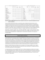
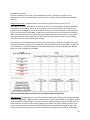
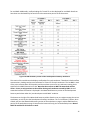
Stormwater Ordinance Appendix
APPENDIX O
FALLS LAKE STORMWATER
LOAD ACCOUNTING TOOL
Developers and designers should use the Falls/Jordan Stormwater Accounting Tool
spreadsheets provided by NCDENR DWQ, available online at:
http://portal.ncdenr.org/web/wq/ps/nps/fallslake
Franklin County Stormwater Ordinance
Stormwater Accounting Tool
Jordan/Falls Lake Stormwater Load Accounting Tool
(Version 1.0)
User’s Manual
(revised January 31, 2011)
share.triangle.com
1
Introduction
This accounting tool was developed by North Carolina State University in coordination with NCDENR to
be used with the Jordan Lake Nutrient Strategy Rules. While the original application of this tool is the
Jordan Lake Nutrient Strategy, it may also be applied to any location within the state of North Carolina.
This tool is intended to be used for new developments (NCDENR is developing a separate tool for
existing developments within the Jordan Lake watershed), but can be also be applied to existing
developments that are incorporating retrofit best management practices (BMPs).
Important Notes:
Some BMPs included in the tool may not currently be used for meeting nutrient reduction
requirements. Please check with the Division and the Division’s Stormwater BMP Manual for more
details.
While the tool provides the option of undersizing BMPs, this option cannot currently be used to meet
the Jordan New Development requirements. This option may potentially be used if the tool is used to
calculate nutrient reductions for retrofits on existing development.
Using the Client/Master Files
To prevent manipulation of the Jordan/Falls Lake Stormwater Load Accounting Tool (JLSLAT) and its
outputs, a system has been developed involving two Excel files: a Client file and a Master file. The Client
file will be distributed to the general public and the Master file will be distributed to regulators by
NCDENR. The Master file is NOT designed to run scenarios and analyze developments. Its only use is for
regulators to extract input data from the Client file and view results. To ensure that both files function
properly and produce accurate results, do NOT attempt to change any formatting, data or formulas
within the files.
Client File
Developers (or anyone submitting the results from the JLSLAT for regulatory review) may use the Client
file to run any and all scenarios for a given development. When they are ready to submit a given
scenario/development for review, they will save the Client file and send it to the appropriate regulatory
agency. The agency’s Master file will extract the input data from the Client file and produce its own
results. Regulators will use these results to review the development.
Master File
The Master file extracts the input data from a specified Client sheet and produces its own set of results.
Again, the Master file is NOT designed to run scenarios and analyze developments. It is strongly
recommended that the regulatory agency use the “Save As” feature to have a separate Master file for
each Client file. To establish the connection between the Master and Client files, go to the Instructions
worksheet and click on Data Connections Edit Links. Browse files and select the client sheet you
want to extract the data from. Click on the Update Values button. The files should update automatically
and any time the Master Sheet is opened it will extract the data from the specified Client file. You may
check the status of the connection by clicking Data Connections Edit Links Check Status. If for
some reason the link is broken, simply repeat the steps described above.
2
Glossary of Terms
water quality depth – The depth of rainfall that a BMP is designed to capture and treat (generally 1 inch
for all regions except CAMA; for CAMA, it is generally 1.5 inches).
physiographic region – Broad-scale subdivision based on terrain texture, rock type and geologic
structure and history. In North Carolina, there are five main physiographic regions: coastal plain,
sandhills, piedmont, Triassic basin, and mountains. (In the JLSAT, the region “CAMA” refers to the region
of the state where Coastal Area Management Act applies – see NCDENR’s website for more information
about this region and the stormwater requirements)
hydrologic soil group – Soils are classified into hydrologic soil groups (HSGs) to indicate the minimum
rate of infiltration obtained for bare soil after prolonged wetting.
median effluent concentration – The median concentration of a given constituent that is released from a
best management practice. This value is independent of the inflow concentration.
internal water storage zone – Subsurface portion of a bioretention cell that provides water storage in
the bottom of the cell. Water stored in this layer is principally released by exfiltration. The IWS zone is
created by elevating the underdrain, usually with a 90-degree PVC elbow.
3
I. Using the Jordan/Falls Lake Stormwater Load Accounting Tool (JLSLAT)
This section covers the use and interpretation of the JLSLAT. There are four worksheet tabs within the
Excel spreadsheet that users will need to access: Instructions, Watershed Characteristics, BMP
Characteristics, and Development Summary. The Instructions tab provides background information and
general instructions for using the JLSLAT. The Watershed Characteristics and BMP Characteristics tabs
allow users to enter their development and BMP data. Finally, the Development Summary is where all
outputs are displayed. Users may navigate between these four tabs by either clicking the buttons at the
top of the worksheets (Figure 1A) or by clicking on the tab name at the bottom of the screen (Figure 1B).
Each tab and its corresponding instructions, assumptions and uses are discussed in the next four
sections.
Figure 1. Methods of navigating between worksheet tabs.
Instructions
The Instructions tab is the first worksheet one sees when opening the JLSLAT Excel file. This tab contains
all instructions and assumptions regarding the JLSLAT and its use. Specific instructions are stated again
in subsequent tabs so users can refer to them easily.
This worksheet contains two maps: a physiographic region map (Figure 2) and an annual precipitation
map (Figure 3). These maps are provided for users to reference when choosing their physiographic
region and precipitation location on the “Watershed Characteristics” tab. There is also a table (Table 1)
of counties located within, or partially within, each physiographic region. Table 1 allows users to get a
general idea of what region their site is located in. For users whose county is located within multiple
regions, it is crucial that they determine which region the site of interest pertains to, as this affects
calculations and outputs from the JLSLAT. This will be discussed in greater detail in the “Watershed
Characteristics” section.
Cells shaded grey are those designated for data input.
4
Figure 2. Map of physiographic regions within the state of North Carolina (also located in the JLSLAT
on the Instructions worksheet).
Figure 3. Average annual precipitation map for the state of North Carolina. Labeled towns/cities are
available in the dropdown menu for ‘precipitation location’ (also located in the JLSLAT on the
Instructions worksheet).
5
Table 1. List of counties located within, or partially within, each physiographic region.
PIEDMONT & MOUNTAIN
Rockingham
Alamance
Alexander
Alleghany
Anson
Ashe
Avery
Buncombe
Burke
Cabarrus
Caldwell
Caswell
Catawba
Chatham
Cherokee
Clay
Cleveland
Davidson
Davie
Durham
Forsyth
Franklin
Gaston
Graham
Granville
Guilford
Halifax
Harnett
Haywood
Henderson
Iredell
Jackson
Johnston
Lee
Lincoln
Macon
Madison
McDowell
Mecklenburg
Mitchell
Montgomery
Moore
Nash
Northampton
Orange
Person
Polk
Randolph
Richmond
Rowan
Rutherford
Stanley
Stokes
Surry
Swain
Transylvania
Union
Vance
Wake
Warren
Watauga
Wilkes
Wilson
Yadkin
Yancey
COASTAL
PLAIN
CAMA
COUNTIES
TRIASSIC
BASIN
Bladen
Columbus
Cumberland
Duplin
Edgecombe
Halifax
Harnett
Hoke
Johnston
Jones
Martin
Moore
Nash
Northampton
Pitt
Richmond
Robeson
Sampson
Scotland
Wake
Wayne
Beaufort
Bertie
Brunswick
Camden
Carteret
Chowan
Craven
Currituck
Dare
Gates
Hertford
Hyde
New Hanover
Onslow
Pamlico
Pasquotank
Pender
Perquimans
Tyrrell
Washington
Durham
Granville
Wake
Chatham
Lee
Moore
Montgomery
Richmond
Anson
Union
Rockingham
Stokes
Davie
SANDHILLS
Montgomery
Moore
Lee
Harnett
Cumberland
Hoke
Robeson
Scotland
Richmond
6
Watershed Characteristics
On the Watershed Characteristics worksheet users enter all information pertaining to the site of
interest, including both pre- and post-developed conditions. General development information is
entered in the upper section of the worksheet (shown in Figure 4).
Figure 4. General development information section of Watershed Characteristics worksheet.
•
•
•
•
•
•
Physiographic/Geologic Region (required): This is the physiographic region in which the site is
located. Select the appropriate region from the drop-down menu. Regions to select from
include: CAMA (coastal area management act), Coastal, Sandhills, Piedmont, Triassic Basin, and
Mountains. Users may reference Figure 2 or Table 1 (both located in the Instructions worksheet)
to determine the appropriate physiographic region. The region of a site dictates the volume
reduction capabilities of BMPs.
Hydrologic Soil Group (required): The hydrologic soil group (HSG) is the predominant type of soil
located on the site. Select the appropriate HSG (A, B, C or D) from the drop-down menu. Users
may use on-site soil tests or soil maps to determine the appropriate HSG; however, one must be
careful that the HSG does not vary throughout the site and truth-checking soil maps is highly
encouraged (sometimes required). The HSG is a reference for regulators to make sure the
selected BMPs are acceptable for the given HSG.
Precipitation Location (required): Users should select a location from the drop-down menu that
most closely represents the rainfall patterns of the site. Note that this may not necessarily be
the closest location to the site. Figure 3 shows trends for North Carolina regarding average
annual rainfall depths and can be used to choose the most appropriate precipitation location.
The location selected is used to determine stormwater runoff volumes for the site.
Total Development Area (required): Enter the total number of square feet comprising the site to
be analyzed. It is important that this value equal the sum of all areas entered in the pre- and
post-development land use columns. In the event that these values do not match, a warning will
appear at the bottom of the worksheet alerting the user of this fact.
Development Name (optional): The name assigned to the site/development to be analyzed. This
name will appear on the summary sheet with the JLSLAT outputs.
Model Prepared By (optional): The name of the person using the JLSLAT for a site/development.
This name will appear on the summary sheet with the JLSLAT outputs.
The lower section of the Watershed Characteristics worksheet (Figure 5) is where users enter land use
data for pre- and post-development conditions.
7
Figure 5. Section of Watershed Characteristics worksheet where pre- and post-development land use
areas are entered.
Users may enter land use information in two sections: Non-residential land uses (Column 1) and
residential land uses (Column 2). Land uses associated with commercial, industrial, or transportation
categories are listed on the left of the screen, while land uses associated with the residential category
are found on the right of the screen. Miscellaneous pervious land uses, as well as land that is taken up
by BMPs, are also listed in the non-residential section of this worksheet. Land areas designated to BMPs,
whether they exist in pre-development conditions, or whether they will be incorporated with the
development, should be entered in the “Land Taken Up By BMPs” category. Natural wetlands, riparian
buffers and open water (dubbed “Jurisdictional Land Uses”) are included in the model; however, these
land uses are not considered in the runoff volume or concentration calculations, nor may they be
treated by BMPs.
Land area values do not have to be entered in only one of the columns – they may be mixed among
the two columns if necessary.
Users should enter the total area within the site/development for each type of land use. This should be
done for both pre- and post-development conditions. If a particular land use is not present on the site,
the cells may be left blank or a zero may be entered. The TN EMC and TP EMC values listed beside each
land use are the representative concentrations of total nitrogen (TN) and total phosphorus (TP) found in
stormwater runoff leaving that particular land use. The methods used to establish percent impervious
assignments and representative pollutant concentrations for individual land uses are discussed in Part II
of this document. The percent impervious value for the driveway land use is adjustable. This value
defaults to 1 (100% impervious); however uses may adjust this in the gray-shaded cell in the “Age of
Development” column. Note that the percent impervious value entered must be validated and may or
may not be accepted by the reviewing agency.
It is important that the areas entered for both the pre- and post-development condition sum to equal
the “Total Development Area” entered in the upper section of the Watershed Characteristics worksheet.
A chart displaying the totals for each of these values is located below Column 1 (“Land Use Area Check”).
If these values do not equal each other, a warning will be displayed below Column 2 to alert the user
that there is a discrepancy.
8
Residential Land Uses. There are two options for entering land use information for residential sites. The
first option is entering area values in Part A of Column 2. This section gives several lot size options,
including ⅛-, ¼-, ½-, 1- and 2-acre lots, as well as multi-family and townhome lots. If the site conforms to
one of these specific lot sizes, the appropriate area may be entered in the gray-shaded cells next to the
appropriate land use. Average percent impervious values and representative TN and TP concentrations
for these lot sizes are built in to the JLSLAT. The method by which these values were determined is
discussed in Part II of this document.
If the site’s lot sizes fall between the given lot sizes, users may use the “Custom Lot Size” option. To do
so, the user will enter the lot size for the development in the gray-shaded cell in the “Custom Lot Size”
column. This value must fall between ⅛ acre and 2 acres, as the JLSLAT linearly interpolates the percent
imperviousness and representative pollutant concentrations from the given lot sizes. If the values fall
outside this range, or the user prefers (or is required) to report individual residential land uses within a
development, Part B of Column 2 should be used. Part B lists out all types of land uses that may be
found within a residential area and allows the user to enter the total number of acres of each land use
present for the site of interest.
To avoid inaccurate results, do NOT list out individual land uses in Part B
within an area already described by lot size in Part A.
When using Part A of Column 2 to enter land use area information, users must specify the age of the
development in the column labeled “Age of Development”. It is expected that the majority of
developments analyzed with the JLSLAT will be new developments; however, should the JLSLAT be
applied to existing developments, users have the option of choosing an age of “Before 1995” and “After
1995”. For new developments, users should select “New”. Results will not be displayed if a
development age is not selected.
Users may clear all entries by clicking the “Clear All Values” button at the top of the worksheet. The
other buttons – “Return to Instructions”, “Proceed to BMP Characteristics” and “Skip to Summary Page”
– allow users to navigate among the different worksheets. In order for the “Clear All Values” button to
work, macros MUST be enabled. An additional note regarding the “Clear All Values” button: When using
the Client and Master files, clicking the “Clear All Values” button in the Master file will only clear values
that were entered in the Master file in addition to those values carried over from the Client file. All
values that were entered in the Client file (and thus carried over to the Master file) will remain. To clear
these values, the user must click the “Clear All Values” button in the Client file. To avoid confusion, it is
best to work entirely within the Client File. It is unnecessary to perform any actions within the Master
file.
BMP Characteristics
All details pertaining to the BMPs that will be used to treat runoff from the development are entered in
the BMP Characteristics worksheet. Users may divide the development into as many as 6 catchments,
and each catchment may be treated with up to 3 BMPs.
BMPs are selected by clicking on the appropriate cell in the row of the worksheet labeled “BMP Type”
(indicated by an arrow in Figure 6). After clicking on the cell, an arrow will appear on the right side of the
cell. Click this arrow and a dropdown menu will appear with the available BMP choices: Bioretention
9
with IWS (Internal Water Storage Zone), Bioretention without IWS, Dry Detention Pond, Grassed Swale,
Green Roof, Level Spreader/Filter Strip, Permeable Pavement, Sand Filter, Water Harvesting, Wet
Detention Pond, and Wetland. Click on the appropriate BMP. To clear a BMP choice, either click on the
cell and press the ‘delete’ key, or select the blank row in the dropdown menu.
If more than 1 BMP is assigned to a single catchment, the BMPs are assumed to operate in series
(i.e. the outflow from BMP 1 flows into BMP 2, etc.)
The JLSLAT allows the user to designate additional drainage areas for the second and third BMP in the
series. If additional drainage area was designated for BMP 2 of the series, BMP 2 would treat not only
the outflow from BMP 1, but also the runoff from the designated drainage area. To designate this
additional drainage area, simply enter the square footage for each type of land use within the area in
the column for BMP 2 (more details on how to specify land uses within BMP drainage areas will be
provided later in this section).
Figure 6. Section of the BMP Characteristics worksheet where information regarding type of BMP,
undersizing/oversizing and catchment routing is entered.
Undersized BMPs. The JLSLAT allows for BMPs to be undersized to a minimum of 50% of the size
required to treat the water quality event. When a BMP is undersized, the volume reduction provided by
the BMP is reduced using a 1:1 ratio (i.e. if the BMP size required to treat the water quality event is
reduced by 40%, the assigned volume reduction will be reduced by 40%). However, the median effluent
concentrations assigned to the BMP remain the same. To specify that a BMP is undersized, the user
should enter the BMP's size relative to the design size required to capture the designated water quality
depth in decimal form (i.e. 75% of required design size = 0.75) in the appropriate row of the worksheet
(circled in Figure 6). (While the tool provides the option of undersizing BMPs, this option cannot
currently be used to meet the Jordan New Development requirements. This option may potentially
be used if the tool is used to calculate nutrient reductions for retrofits on existing development –
check with DWQ.)
10
Oversized BMP. The JLSLAT does not include a direct method of oversizing BMPs; however, users can
model oversized BMPs. To do so, users must enter two BMPs of the same type in series (the outflow
from the first BMP flows into the second BMP). The BMP type should be that of the BMP the user wishes
to oversize. The percent by which the user wishes to oversize the BMP should be added to 100%, then
divided by 2. This value will be entered in the same row that undersized values are entered (circled in
Figure 6) for both BMPs. For example, if a BMP was to be 50% greater than the size required to treat the
water quality depth, it would be a total of 150% of the design size. Divide this value by 2, and the two
BMPs in series would be assigned an ‘undersized’ value of 0.75 each.
Catchment Routing. Any catchment within the development may be routed to any other BMP or
catchment. The section in which this information is entered is highlighted by a box in Figure 6. To
indicate that a BMP is accepting the outflow from another catchment, select “yes” from the dropdown
menu in the cell corresponding to the BMP that is accepting the outflow. For example, if BMP 2 of
Catchment 1 is accepting the outflow from Catchment 3, the cell corresponding with the column for
BMP 2 of Catchment 1 and the row for Catchment 3 should be changed to display “yes” instead of “no”.
To route one catchment to another catchment, simply route the catchment outflow to the first BMP
within the catchment accepting the outflow.
Water Harvesting BMP. Water harvesting is a BMP given as an option within the JLSLAT. Users must
enter a volume reduction for the water harvesting BMP in the appropriate row within the BMP
Characteristics worksheet. This is the volume reduction used to calculate volume and nutrient outputs
from the system. It is important to note that the water harvesting BMP is NOT modeled as a catch-andrelease system in the JLSLAT; it is assumed that volumes reduced by the system are NOT released to the
stormwater network. It is up to the developer to prove that this is in fact the case and that the reported
volume reduction is accurate.
To aid with the selection of BMPs, a table (“BMP Details”) is located at the top of the worksheet and
displays the volume reduction and median effluent concentrations for each type of BMP for the
physiographic region indicated in the Watershed Characteristics page. (Note the values will change if the
region is changed.) Figure 7 shows this table with the Coastal physiographic region as the selected
region. Users may use this table to determine which types of BMPs would provide the most treatment
for their development. As permeable pavement, green roofs and water harvesting BMPs are not
assigned a nutrient removal credit, their effluent concentrations default to the value of the land use
they are replacing (parking lot, roof, etc.). (Water harvesting, permeable pavement and green roofs
may not currently be used for meeting nutrient reduction requirements in the Jordan Lake
watershed. Please check with the Division and the Division’s Stormwater BMP Manual for
applicability details.)
11
Figure 7. “BMP Details” table displaying values for the Piedmont physiographic region (blank cells
indicate 0% volume reduction).
The lower portion of the BMP Characteristics worksheet (Figure 8) allows the user to define the
watershed draining to each BMP. The user should enter the total area of each land use type that drains
to each BMP in the appropriate column. Note that when entering residential land use information the
user MUST be sure to enter the land area values in the appropriate row for the age of the
development (New, Before 1995 and After 1995 ages are listed out separately, unlike the Watershed
Characteristics worksheet). The size of the BMP itself should be entered in the very last land use row –
“Land taken up by BMP” – as all of the rainfall that falls on the BMP enters the BMP.
The areas entered in a given land use MUST be less than or equal to the total area of that land use
entered in the Watershed Characteristics worksheet.
To ensure this is the case, there is a built-in check in the worksheet. If the user enters a value that
exceeds the total available area of that particular land use, the model displays an error message.
However, in order for this check to function, users must press the “Enter” key on the keyboard after
entering the land use area; clicking on a different cell will NOT trigger the check to occur.
The two columns to the right of the Catchment 6 area show the user how many acres of a given land use
are available and how many are currently being treated. The two rows below the grey-shaded cells
shows how many total acres are being treated by each BMP as well as by the series. Remember that
entering land areas for BMPs 2 or 3 in a series indicate that the BMP is accepting runoff from this area
IN ADDITION TO the outflow from the previous BMP. Not all of the watershed must be treated by a
BMP; the Jordan Lake Nutrient Strategy requirements will dictate how much treatment needs to be
included.
Two other checks have been incorporated into the BMP Characteristics worksheet. The first displays a
warning message if a BMP is specified but there are no land areas entered. This prevents the user from
inadvertently erasing land use areas and forgetting to the clear the BMP selection. The second warning
is displayed if a BMP has not been selected but another catchment is being routed to it. Again, this is in
12
case the user forgets to clear the catchment routing after a BMP is removed. To clear all entries in this
worksheet, both land areas as well as catchment routing and BMPs, click the “Clear All Values” button at
the top of the worksheet. In order for the “Clear All Values” button to work macros, MUST be enabled.
Figure 8. Section of the BMP Characteristics worksheet where information regarding land use of BMP
drainage area(s) is entered.
13
Development Summary
The final worksheet in the JLSLAT is the Development Summary; it displays all outputs for the
development of interest. The worksheet is separated into 2 sections: Watershed Summary and BMP
Summary.
Watershed Summary. The Watershed Summary section (Figure 9) displays outputs for ‘predevelopment’ and ‘post-development’ conditions, as well as ‘post-development’ conditions with BMPs
incorporated. These outputs include percent impervious, annual runoff volume, TN median effluent
concentration, TN loading rate, TP median effluent concentration and TP loading rate. Values reported
for the ‘post-development with BMPs’ condition account for portions of the watershed not treated by
BMPs. The Documentation portion of this document explains how each of these values are calculated.
The watershed TN and TP loading values are those that correspond with the required target loading
rates set forth by the Jordan Lake Nutrient Strategy.
The lower portion of the Watershed Summary section reports percent differences between the various
watershed conditions, including ‘pre-development’ and ‘post-development’ without BMP incorporation,
‘pre-development’ and ‘post-development’ with BMP incorporation, and ‘post-development’ without
BMPs, and ‘post-development with BMPs’.
Figure 9. Watershed Summary section of the Development Summary worksheet.
BMP Summary. The BMP Summary section of the Development Summary (Figure 10) worksheet displays
information regarding the BMPs treating the development. The total area treated by each BMP includes
the area treated by previous BMPs in the series, as well as additional area draining to the BMP itself. The
inflow volume is the total amount of water flowing into the BMP. The percent volume reduction is the
volume reduction potential assigned to the BMP types within the specified physiographic region (the
same value displayed in Figure 7). The inflow concentrations and loadings for TN and TP are displayed
14
for each BMP. Additionally, outflow loadings for TN and TP are also displayed for each BMP. Details on
how these are calculated may be found in the Documentation portion of this document.
Figure 10. BMP Summary section of the Development Summary worksheet.
This section of the worksheet also displays outflow data for each catchment. These data include outflow
concentrations, loadings and percent reductions for TN and TP for each catchment. The last BMP in each
of the series releases water of this quality and these values account for any catchment routing that is
specified in the BMP Characteristics tabs. Note that these values are NOT the watershed outflow
values – these are only pertinent to the outflow leaving each catchment treated by BMPs. Overall
watershed outflow information is displayed in the Watershed Summary section of the Development
Summary worksheet under the ‘post-development with BMPs’ condition.
The buttons to the right of the Watershed Summary tables allow the user to navigate among the various
worksheets, as well as print the Development Summary worksheet. The “Print Summary” button, when
clicked, will print the Watershed Summary portion of the worksheet on page 1 and the BMP Summary
portion of the worksheet on page 2. Note that the button will only print to the default printer. Macros
MUST be enabled for this button to work.
15
II. Model Documentation
Governing Principles and Limitations
Calculations performed within the model are governed by two basic principles: Simple Method (for
runoff volume and pollutant loading calculations) and the median effluent concentration BMP efficiency
metric (for BMP reduction calculations). Each of these principles is described below.
Simple Method
The Simple Method is a method for estimating the volume of stormwater runoff and the pollutant load
exported within that runoff leaving a small urban catchment. Volume calculations are based upon
impervious cover of a catchment, which is represented by the runoff coefficient Rv:
Rv = 0.05 + (0.009 * I)
(1)
where Rv = Simple Method runoff coefficient; and
I = percent impervious cover of the catchment (%).
The volume is a function of the runoff coefficient, Rv, the area of the catchment and the annual rainfall
amount. Some variations of the Simple Method are applied on an individual storm basis, in which case
the precipitation value would be the depth of rainfall that one wishes to estimate runoff for. For JLSLAT
applications, annual precipitation values are used.
V = Rv * A * (P/12)
(2)
where V = volume of runoff (ft3),
A = area of catchment (ft2), and
P = average annual rainfall depth (in).
To estimate the mass of pollutant that leaves the catchment on an annual basis, Equation 3 is used.
L = (P * Pj * Rv) ÷ (12 * C * A *2.72)
(3)
where L = average annual pollutant load (lbs),
Pj = fraction of rainfall events that produce runoff, and
C = event mean concentration of the pollutant (mg/L).
CWP, 2007 recommends a Pj value of 0.9, indicating that 90% of rainfall events produce runoff.
However, for the JLSLAT a value of 1.0 was used in order to provide a conservative estimate of the
pollutant load leaving the site. The event mean concentrations used for certain land uses will be
discussed in detail in the “Watershed Characteristics” section of this document.
Several assumptions/limitations accompany the Simple Method (taken from CWP, 2007):
(1) The Simple Method should be used on catchments with areas of 1 square mile (640 acres) or
less; and
(2) The Simple Method only estimates pollutants loads leaving the catchment via stormwater
runoff.
16
Determining Representative Pollutant Concentrations for Various Types of Land Uses
A literature review was conducted to establish representative pollutant concentrations for various land
use types. Only peer-reviewed literature was considered in this endeavor; however, geographic
limitations were not imposed. Only data that were reported for the specific land use of interest (i.e. not
multi-use watersheds) were used. If multiple data were available, the average of the data was taken as
the representative pollutant concentration (unless otherwise noted). Table 2 displays the representative
TN and TP concentration values for various land uses, as well as the references from which the values
were derived. Raw data from individual studies used to compute these values may be found in Appendix
A.
Determining Percent Imperviousness for Various Residential Lot Sizes
This section was compiled by the Center for Watershed Protection, Inc. (the Center) and presents the
methodology for identifying types of impervious cover (IC) in suburban residential land uses. The
polygons used in this study were suburban in nature and most of the development was constructed
after 1970 and before 2001. Although these estimates were developed using data from the Chesapeake
Bay region, it is assumed that these numbers provide a reasonable estimate suburban development
trends that can be transferred to other regions outside this watershed. However, the IC estimates
presented herein apply to recent suburban development, and may not be transferrable to ultra-urban or
older development areas.
Using GIS data from Baltimore County (MD), Howard County (MD), James City County (VA), and
Lancaster County, (PA), the Center analyzed IC coefficients for single family residential suburban land
uses. Homogenous land use polygons were analyzed using Geographic Information Systems (GIS) data.
Land use polygons were defined using the descriptions presented in Table 3.
The following criteria were used to select single family residential polygons for analysis:
• For residential land uses, the parcel boundary information was used to first classify parcels
based on acreage (shown in the description in Table 3). Development patterns that most
closely matched the land use category (e.g., ¼ acre lots) were selected for sampling. Because
most subdivisions do not have uniform lot sizes, subdivisions were selected if the majority of
lots or average lot size met the general criteria for the land use category.
• Because of difficulty in finding subdivisions that met the above criteria for polygon
delineation, no minimum area was set for the polygon size for residential areas. Instead, it
was decided that each residential polygon must include a minimum of 5 lots.
• Polygons were drawn by following the lot lines of contiguous parcels and excluding areas of
“unbuildable” land located in the interior of the polygon. Stream valleys that did not
originate within the subdivision were excluded from the land use polygons, as were other
“unbuildable” lands such as floodplains, wetlands, and conservation areas. The basis behind
this rule is that not all development sites include these types of characteristics. When
predicting future impervious cover, a planner could estimate the areas based on existing
mapping and based on local codes and ordinances that determine “unbuildable” acreage.
This acreage could then be removed from the total acreage of the planning area.
• Stormwater ponds and open water were not considered to be impervious cover because they
are generally small in area and are not always associated with a single land use. While water
surfaces do act as impervious surfaces in a hydrologic sense, they do not generally have
similar consequences on stream quality, watershed health, or pollutant loading as more
conventional impervious cover such as roads, parking lots, and rooftops.
17
Table 2. Representative TN and TP concentrations for various land uses.
TN
TP
Land Use Type
Reference
(mg/L)
(mg/L)
Residential
Driveway
1.44
0.39
Passeport et al. (2009) (using industrial values)
Roof
1.08**
0.15* *Moran (2004) and Bannerman (1993) **Moran (2004)
Lawn
2.24
0.44
Skipper (2008) and NCDENR Tar-Pam Model
Commercial/Ultra-Urban
Parking lot
1.44**
0.16* *Bannerman (1993) and Passeport et al. (2009); **Passeport et al. (2009)
Roof
1.08**
0.15* *Moran (2004) and Bannerman (1993), **Moran (2004)
Open/Landscaped
2.24
0.44
Skipper (2008) and NCDENR Tar-Pam Model
Industrial
Parking lot
1.44**
0.39* *Bannerman (1993); **Passeport et al. (2009)
Roof
1.08**
0.15* *Moran (2004) and Bannerman (1993), **Moran (2004)
Open/Landscaped
2.24
0.44
Skipper (2008) and NCDENR Tar-Pam Model
Transportation
High density (interstate, main)
3.67
0.43
Wu et al. (1998), urban
Low density (secondary, feeder)
1.4
0.52
Wu et al. (1998), semi-urban
Rural
1.14
0.47
Wu et al. (1998), rural
Sidewalks
1.43**
1.16* *Bannerman (1993); Passport et al. (2009)
Other
Woods
1.47
0.25
Line et al. (2002) median
Maintained grass
3.06
0.59
Skipper (2008)
Pasture
3.61
1.56
Line et al. (2002) median
18
Table 3. Land Use Categories and Descriptions
Residential Land Use
Description
2 Acre Lots
Lot size ranges from 1.70 to 2.30 acres
1 Acre Lots
Lot size ranges from 0.75 to 1.25 acres
1/2 Acre Lots
Lot size ranges from 0.40 to 0.60 acres
1/4 Acre Lots
Lot size ranges from 0.20 to 0.30 acres
Lot size ranges from 0.10 to 0.16 acres, includes
1/8 Acre Lots
duplexes
5-10 units/acre, attached single family units that
Townhomes
include a lot area
10-20 units/acre, residential condominiums and
Multifamily
apartments with no lot area associated with the
units
Once a development area was selected, the criteria used to delineate the polygons were generally as
follows:
• Parcel lines were used as guides for drawing the polygon boundaries.
• “Unbuildable” land such as floodplains, steep slopes, and conservation areas were not
included in the polygons.
• Subdivision lots that were not built out were not included in the polygons.
• Large forested areas located outside parcel boundaries were not included in the polygons.
• Local and arterial roads were included in the polygons if the parcels bordering each side of
the road had the same land use.
• If a local or arterial road bordering a parcel had a different land use bordering the other side
of the road, only half the road was included in the polygon. Interstate and state highways
were not included in the polygons.
• Parcel data such as a business or owner name was used to verify land use.
• Orthophotos were also used to verify land use.
A direct measurement technique was used to assess the IC for each land use polygon. This involved
clipping planimetric IC layers (e.g., buildings, roads, parking lots) to the land use polygons using GIS. For
IC types not available as planimetric data (e.g., sidewalks, driveways), the following major assumptions
were made:
Other Impervious Surfaces
Orthophotos were used to digitize an impervious cover layer that included tennis courts,
garages, and other impervious surfaces not included in the buildings, parking lots, roads,
driveways, or sidewalks layers. This layer was included in the processing and calculation of total
impervious cover.
Sidewalk Estimation
Sidewalks were identified only as lines in the GIS layers, so orthophotos were used to measure
the length of sidewalks in each polygon, which was then multiplied by 4 feet (assumed sidewalk
width). The resulting numbers were added to the data table for calculation of total impervious
cover.
19
Driveway Estimation
Driveway data was not available so GIS orthophotos were used to determine an average
driveway size for each polygon, which was then multiplied by the number of homes within the
polygon. The resulting numbers were added to data table for calculation of total impervious
cover.
Results for each land use polygon were used to compute an average IC by type for various suburban
residential land uses. More detailed information on the sampling protocol and impervious cover
measurement can be found in Cappiella and Brown, 2001.
The current zoning code classifications for the City of Durham, NC are shown in Table 4. The information
in this table can be used to guide the application of the IC coefficients to residential zoning
classifications in North Carolina.
Table 4. Zoning Classifications for Durham, NC (City of Durham, N.C.)
Durham Zoning
Minimum Lot
Minimum Lot Area
Equivalent Land Use
Code
Area
(acre)
from Analysis
(square feet)
R-20
20,000
0.46
1/2 ac
R-15
15,000
0.34
R-10
10,000
0.23
1/4 ac
R-8
8,000
0.18
R-5
5,000
0.11
1/8 ac
R-3
3,000
0.07
The results of the analysis are presented in Table 5. For single family residential categories, driveways
consistently made up about 4% of the polygon area, while roads and buildings comprised an equal
percentage that progressively increased with development density. Sidewalks in residential areas
composed from <1% to 2% of the polygon area, and this number also increased with development
density.
Table 5. Results of the IC Analysis by Land Use and Type of IC
Number
Total
%
%
%
%
%
% Other
Land Use
of
% IC
Roads Buildings Parking Driveways Sidewalks Impervious
Polygons
2 Acre Lots
12
10.6%
3.4%
3.3%
0.0%
3.8%
0.0%
0.1%
1 Acre Lots
23
14.3%
4.8%
5.1%
0.0%
4.1%
0.1%
0.2%
1/2 Acre Lots
20
21.2%
7.5%
7.9%
0.0%
4.4%
1.2%
0.2%
1/4 Acre Lots
23
27.8%
10.8%
11.0%
0.0%
4.4%
1.6%
0.1%
1/8 Acre Lots
10
32.6%
13.4%
12.2%
0.0%
4.7%
2.2%
0.0%
Townhomes
20
40.9%
12.6%
16.4%
6.4%
2.1%
2.7%
0.6%
Multifamily
18
44.4%
13.1%
15.9%
13.0%
0.0%
1.4%
1.0%
20
Determining Percent Imperviousness for Residential Lots of Various Ages
This section was compiled by the Center for Watershed Protection, Inc. (the Center) and presents the
methodology for identifying impervious cover (IC) values in suburban residential land uses for a
sampling of developments in four age ranges: developments built prior to 1995 (older than 15 years),
developments built after 1995 (0-15 years old), developments built prior to 1985 (older than 25 years)
and developments built after 1985 (0-25 years old).
The land use polygons used in this study were suburban in nature and most of the development was
constructed after 1970 and before 2005. Although these estimates were developed using data from the
Chesapeake Bay region, it is assumed that these numbers provide a reasonable estimate of suburban
development trends that can be transferred to other regions outside this watershed. The IC estimates
presented herein apply to relatively recent suburban development, and may not be transferrable to
ultra-urban or older development areas.
Using GIS data from Frederick County, MD, the Center analyzed IC coefficients for single family
residential suburban land uses. Homogenous land use polygons were analyzed using Geographic
Information Systems (GIS) data. Land use polygons were defined using the descriptions presented in
Table 6.
Table 6. Land Use Categories and Descriptions
Residential Land Use
Description
Very Low Density Residential Lot sizes greater than 1 acre (less than 1 dwelling
(VLDR)
unit per acre)
Low Density
Lot size ranges from 0.25 to 1 acre (1 to 4 dwelling
Residential (LDR)
units per acre)
Medium Density Residential Lot size ranges from 0.1 to 0.2 acres (5 to 10
(MDR)
dwelling units per acre)
High Density
Lot sizes less than 0.1 acre (greater than 10 dwelling
Residential (HDR)
units per acre)
The current zoning code classifications for the City of Durham, NC are shown in Table 7. The information
in this table can be used to guide the application of the IC coefficients to residential zoning
classifications in North Carolina.
Table 7. Zoning Classifications for Durham, NC (City of Durham, N.D.)
Durham Zoning
Minimum Lot
Minimum Lot Area
Equivalent Land Use
Code
Area
(acre)
from This Analysis
(square feet)
R-20
20,000
0.46
LDR
R-15
15,000
0.34
LDR
R-10
10,000
0.23
LDR
R-8
8,000
0.18
MDR
R-5
5,000
0.11
MDR
R-3
3,000
0.07
HDR
21
The following criteria were used to select residential polygons for analysis:
•
Residential polygons were selected at random by using a Random Number Generator in Excel to
assign a numerical number to each subdivision in the County’s GIS data. The random selection
process was limited to subdivisions built after 1973. Subdivisions were then analyzed in numerical
order of the random numbers.
•
For each subdivision, the parcel boundary information was used to first classify parcels based on
acreage (shown in the description in Table 6). Development patterns that most closely matched the
land use category (e.g., ¼ acre lots) were selected for sampling. Because most subdivisions do not
have uniform lot sizes, subdivisions were selected if the majority of lots or average lot size met the
general criteria for the land use category.
•
Because of difficulty in finding subdivisions that met the above criteria for polygon delineation, no
minimum area was set for the polygon size for residential areas. Instead, it was decided that each
residential polygon must include a minimum of 5 lots unless it was in the very low density residential
category.
•
Stormwater ponds and open water and pools were not considered to be impervious cover because
they are generally small in area and are not always associated with a single land use. While water
surfaces do act as impervious surfaces in a hydrologic sense, they do not generally have similar
consequences on stream quality, watershed health, or pollutant loading as more conventional
impervious cover such as roads, parking lots, and rooftops.
Once a development area was selected, the following methods were used to delineate land use
polygons:
•
Residential polygons generally included individual lots as well as common land owned by the
homeowner’s association or developer. The subdivision names in the County’s subdivision layer
were used to determine which residential areas to include within a given land use polygon. Lots
that were not yet built were not included as part of the subdivision.
•
Interstate/state highways were not included in the polygons. Interior roads (e.g., subdivision roads)
were included within the land use polygons. Local and arterial roads were included in the polygons if
the parcels bordering each side of the road had the same land use. If a local or arterial road
bordering a parcel had a different land use bordering the other side of the road, only half the road
was included in the polygon.
•
Sample polygons were drawn by following the lot lines of contiguous parcels.
•
After delineating each polygon, the appropriate land use type (i.e., VLDR, LDR, MDR, or HDR) was
assigned. The owner listed in the tax map data, as well as 2007 aerial photos supplied by the County
were used to verify land use.
•
The age range of each neighborhood (0-15 years, 0-25 years, older than 25 years or older than 15
years) was determined by using the build date in the County’s tax map data. Age range was assigned
based on the most common build dates of the lots within each subdivision.
After the delineation of sample polygons, the following methods were used to determine impervious
cover based on residential land use type and age:
•
Impervious cover data was obtained from a 2007 planimetric layer provided by the County. This
layer included impervious cover in the form of buildings, driveways, roads, sidewalks, and parking
lots.
•
The impervious cover data was intersected with the residential sample polygons to determine the
total percentage of impervious cover on each polygon. These percentages were then analyzed by
residential land use type and included the mean, median, minimum, maximum, first and third
22
quartiles, and standard deviation. The results are represented by box and whisker plots, as well as
tables in the following section.
Results of the analysis are shown in Figure 11 below. For neighborhoods older than 15 years, median
impervious cover coefficients were 7.2%, 20.2%, 30.3% and 36.0% for VLDR, LDR, MDR, and HDR,
respectively (Figure 12, Table 8). For neighborhoods newer than 15 years, median impervious cover
coefficients were 2.7%, 27.8%, 36.1% and 35.9% for VLDR, LDR, MDR, and HDR, respectively (Figure 13,
Table 9). With the exception of the VLDR land use, median impervious cover coefficients were greater in
developments newer than 15 years. It should be noted that the number of polygons for the
developments newer than 15 years is relatively small, particularly for the LDR land use category.
Figure 11. Median, 25% quartile (Q1), 75% quartile (Q3), minimum, and maximum values for
neighborhoods older than 15 years.
Table 8. Percent Impervious Cover for Neighborhoods Older than 15 Years
Statistic
Q1
Min
Median
Max
Q3
Mean
STD
n
VLDR
3.4
0.9
7.2
16.3
9.5
7.0
3.9
61
LDR
16.2
5.9
20.2
32.5
24.6
20.0
7.6
19
MDR
26.6
22.1
30.3
39.9
33.4
30.1
5.3
14
HDR
32.1
14.6
36.0
53.6
46.1
37.4
9.9
23
23
Figure 12. Median, Q1, Q3, minimum, and maximum values for neighborhoods newer than 15 years.
Table 9. Percent Impervious Cover for Neighborhoods Newer than 15 Years
Statistic
VLDR
LDR
MDR
HDR
Q1
1.4
24.0
29.7
21.9
Min
0.9
20.2
23.8
15.9
Median
2.7
27.8
36.1
35.9
Max
5.5
29.2
41.5
47.9
Q3
4.0
28.5
37.7
37.6
Mean
3.0
25.7
33.8
32.3
STD
1.7
4.9
6.2
10.7
n
9
3
7
9
In order to increase the sample size for “newer” development, differences between IC values for
neighborhoods newer and older than 25 years were also evaluated. For neighborhoods older than 25
years, median impervious cover coefficients were 8.7%, 16.3%, 30.0%, and 41.7% for VLDR, LDR, MDR,
and HDR, respectively (Figure 14, Table 10). For neighborhoods newer than 25 years, median
impervious cover coefficients were 4.1%, 23.2%, 32.3% and 35.9% for VLDR, LDR, MDR, and HDR,
respectively (Figure 15, Table 11). For this analysis, median impervious cover coefficients for the LDR
and MDR were greater in developments newer than 25 years. Median impervious cover coefficients for
the VLDR and HDR were greater in developments older than 25 years.
24
Figure 13. Median, Q1, Q3, minimum, and maximum values for neighborhoods older than 25 years.
Table 10. Percent Impervious Cover for Neighborhoods Older than 25 Years
Statistic
VLDR
LDR
MDR
HDR
Q1
5.4
12.2
26.6
33.9
Min
1.7
5.9
23.2
24.0
Median
8.7
16.3
30.0
41.7
Max
14.9
30.9
33.3
47.6
Q3
10.4
21.0
31.7
46.5
Mean
8.0
17.3
28.8
38.7
STD
3.4
7.9
5.2
9.8
n
30
9
3
5
25
Figure 14. Median, Q1, Q3, minimum, and maximum values for neighborhoods newer than 25 years.
Table 11. Percent Impervious Cover for Neighborhoods Newer than 25 Years
Statistic
VLDR
LDR
MDR
HDR
Q1
2.1
20.2
27.1
30.8
Min
0.9
7.5
22.1
14.6
Median
4.1
23.2
32.3
35.9
Max
16.3
32.5
41.5
53.6
Q3
7.8
27.6
36.4
41.5
Mean
5.4
23.3
31.7
35.5
STD
3.9
6.3
5.9
10.4
n
40
13
18
27
Based on changes in development patterns over the years, the results showed that older developments
were likely to have lower IC than newer developments; however, this was only true for the MDR and
LDR land use categories. This may be due in part to the range of ages sampled (nothing prior to 1970), or
to changes made by Frederick County MD as a result of a Site Planning Roundtable in 2000, or the
nature of the VLDR category (estate homes). Further analysis is needed to hypothesize the specific
reason for the lack of IC increase for the newer VLDR and HDR land use categories.
The data provided by the Center for Watershed Protection regarding the breakdown of different types
of impervious surfaces within residential land uses were used to calculate a composite pollutant
concentration. The concentrations assigned to a specific land use, coupled with the percent of
watershed comprised of that particular land use, allowed for a weighted average concentration to be
calculated. These results are displayed in Table 12.
26
Table 12. Representative pollutant concentrations for residential land uses of various ages.
2-ac lots
1-ac lots
½-ac lots
¼-ac lots
⅛-ac lots
Townhomes
Multi-family
After 1995
TN
TP
2.22
0.44
2.12
0.43
2.06
0.43
2.00
0.42
1.98
0.43
1.94
0.42
1.92
0.41
Before 1995
TN
TP
2.19
0.43
2.15
0.43
2.11
0.43
2.07
0.43
2.02
0.43
1.94
0.42
1.92
0.41
BMP Efficiency: Median Effluent Concentration Method
There are several methods for quantifying the efficiency of a best management practice (BMP). The
method used by the JLSLAT is based upon a median effluent concentration of a given pollutant for a
given BMP. This value will vary based upon the pollutant and the type of BMP. The concentrations used
for the JLSLAT application will be explained in detail in the “Watershed Characteristics” section of this
document.
To apply this BMP efficiency method, one must know the volume of water flowing into a BMP, the
inflow concentration of the pollutant of interest, the percent of inflow volume that leaves the BMP as
treated outflow and untreated overflow, as well as the outflow pollutant concentration for both of these
outflow components. Assumptions made regarding these variables for the JLSLAT are discussed in detail
in the “Watershed Characteristics” section of this document. Equation 4 is used to calculate total mass
of pollutant leaving the BMP and Equation 5 is used to calculate the percent mass removal by the BMP.
Massout = (ECoutflow* Volumeoutflow * 6.2297E-5) + (ECoverflow * Volumeoverflow * 6.2297E-5)
(4)
where Massout = average annual mass of pollutant leaving the BMP (lbs),
ECoutflow = event median concentration for treated outflow portion of outflow (mg/L),
Volumeoutflow = volume of water leaving the BMP as treated outflow (ft3),
ECoverflow = event median concentration for untreated overflow portion of outflow (mg/L), and
Volumeoverflow = volume of water leaving the BMP as untreated overflow (ft3).
BMP%rem = ((ECinflow*Volumeinflow * 6.2297E-5) - Massout) ÷ (ECinflow*Volumeinflow * 6.2297E-5)*100
(5)
where ECinflow = event median concentration for inflow (mg/L), and
Volumeinflow = volume of water entering the BMP (ft3).
27
There are some assumptions regarding this BMP efficiency metric:
(1) The effluent concentration is the median value of the concentrations exiting the BMP.
This metric does not take into account maximum or minimum concentrations and the
representative EC does not vary with storm size or intensity.
(2) This metric assumes the BMP is designed and constructed appropriately to capture and
treat the first flush (1 inch for non-CAMA locations, 1.5 inch for CAMA locations).
(3) The outflow EC is not dependent upon the inflow EC, nor the inflow volume or outflow
volume.
(4) Due to the nature of the metric, the pollutant removal is controlled primarily by the
volume reduction provided by the BMP; thus, BMPs with higher volume reductions will
have greater pollutant removal capabilities.
Determining BMP Median Effluent Concentrations
A literature review was conducted to establish representative effluent concentrations for the BMPs in
the JLSLAT. Only peer-reviewed literature was considered in this endeavor and only studies conducted in
the Mid-Atlantic states were used (Georgia, South Carolina, North Carolina, Virginia, Maryland). Outliers
were excluded from data sets for each BMP type and the median of the reported effluent
concentrations was calculated. Green roofs, permeable pavement, and water harvesting effluent values
were assumed to be the same as the concentrations entering the BMP. These results are shown in Table
13.
Table 13. Median effluent concentrations assigned to BMPs.
BMPs
TN EMC (mg/L)
Bioretention with IWS
Bioretention without IWS
Dry Detention Pond
Grassed Swale
Green Roof
Level Spreader, Filter Strip
Permeable Pavement
Sand Filter
Water Harvesting
Wet Detention Pond
Wetland
*If replacing commercial parking lot, value is 0.16 mg/L.
0.95
1.00
1.20
1.21
1.08
1.20
1.44
0.92
1.08
1.01
1.08
TP EMC (mg/L)
0.12
0.12
0.20
0.26
0.15
0.15
0.39*
0.14
0.15
0.11
0.12
Volume reductions were an integral part of calculating effluent loads from a given BMP. The volume
reduction values assigned to each BMP type varied based upon the physiographic region. These
assignments are displayed in Table 14 and are expressed as percent of the inflow volume.
28
Table 14. Fate of BMP inflow in terms of treated outflow, overflow and loss via ET/infiltration.
Treated Outflow Bypass (Overflow) Volume Reduction
BMP Type
(%)
(%)
(%)
CAMA Region
Bioretention with IWS
10
10
80
Bioretention without IWS
40
10
50
Dry Detention Pond
80
10
10
Grassed Swale
90
0
10
Green Roof
0
50
50
Level Spreader, Filter Strip
45
5
50
Permeable Pavement
38
2
60
Sand Filter
85
10
5
Wet Detention Pond
75
10
15
Wetland
65
10
25
Coastal Region
Bioretention with IWS
10
10
80
Bioretention without IWS
40
10
50
Dry Detention Pond
80
10
10
Grassed Swale
90
0
10
Green Roof
0
50
50
Level Spreader, Filter Strip
45
5
50
Permeable Pavement
38
2
60
Sand Filter
85
10
5
Wet Detention Pond
75
10
15
Wetland
65
10
25
Mountains Region
Bioretention with IWS
40
10
50
Bioretention without IWS
55
10
35
Dry Detention Pond
90
10
0
Grassed Swale
100
0
0
Green Roof
0
50
50
Level Spreader, Filter Strip
55
5
40
Permeable Pavement
98
2
0
Sand Filter
85
10
5
Wet Detention Pond
80
10
10
Wetland
70
10
20
29
BMP Type
Bioretention with IWS
Bioretention without IWS
Dry Detention Pond
Grassed Swale
Green Roof
Level Spreader, Filter Strip
Permeable Pavement
Sand Filter
Wet Detention Pond
Wetland
Bioretention with IWS
Bioretention without IWS
Dry Detention Pond
Grassed Swale
Green Roof
Level Spreader, Filter Strip
Permeable Pavement
Sand Filter
Wet Detention Pond
Wetland
Bioretention with IWS
Bioretention without IWS
Dry Detention Pond
Grassed Swale
Green Roof
Level Spreader, Filter Strip
Permeable Pavement
Sand Filter
Wet Detention Pond
Wetland
Treated Outflow Bypass (Overflow)
(%)
(%)
Piedmont Region
40
10
55
10
90
10
100
0
0
50
55
5
98
2
85
10
80
10
70
10
Sandhills Region
10
10
40
10
80
10
90
0
0
50
45
5
38
2
85
10
75
10
65
10
Triassic Basin Region
55
10
75
10
80
20
100
0
0
50
75
5
98
2
85
10
85
10
75
10
Volume Reduction
(%)
50
35
0
0
50
40
0
5
10
20
80
50
10
10
50
50
60
5
15
25
35
15
0
0
50
20
0
5
5
15
30
References
Bannerman, R. T., D. W. Owens, R. B. Dodds and N. J. Hornewer. 1993. Sources of pollutants in
Wisconsin stormwater. Water Science Technology. 28(3-5):241-259.
Bass, K. L. 2000. Evaluation of a Small In-Stream Constructed Wetland in North Carolina's Coastal Plain.
M.S. thesis. Raleigh, NC: North Carolina State University, Biological and Agricultural Engineering
Bean, E. Z., W. F. Hunt and D. A. Bidelspach. 2007. Evaluation of four permeable pavement sites in
Eastern North Carolina for runoff reduction and water quality impacts. Journal of Irrigation and
Drainage Engineering. 133(6):583-592.
Cappiella, K. and Brown, K. 2001. Impervious Cover and Land Use in the Chesapeake Bay Watershed.
The Center for Watershed Protection. Ellicott City, MD.
Carleton, J.N. 1997. An Investigation of the Performance of a Constructed Wetland in Treating Urban
Stormwater. M.S. Thesis. Manassas, VA: Virginia Polytechnic Institute and State University,
Department of Environmental Sciences and Engineering,
Center for Watershed Protection (CWP). 2007. Urban stormwater retrofit practices. Urban
Subwatershed Restoration Manual Series. Ellicott City, MD.
Chin, D. A. 2006. Surface water hydrology. In Water resources engineering, 334-606. Upper Saddle River,
New Jersey: Pearson Education, Inc.
City of Durham, NC. No Date. City-County Planning Department. General Zoning Districts. Available
online: http://www.durhamnc.gov/departments/planning/zoneord/section4/Index.cfm
Collins, K. A., W. F. Hunt, and J. M. Hathaway. 2010. Side-by-side comparison of nitrogen species
removal for four types of permeable pavement and standard asphalt in Eastern North Carolina.
Journal of Hydrologic Engineering, 15(6): 512-521.
Hathaway, J.M. and W.F. Hunt. 2008. Field Evaluation of Level Spreaders in the Piedmont of North
Carolina. Journal of Irrigation and Drainage Engineering, 134(4):538-542.
Hathaway, J.M. and Hunt, W.F. 2009. An Evaluation of the Dye Branch Wetlands, Final Monitoring
Report. Raleigh, NC.
<http://www.bae.ncsu.edu/stormwater/PublicationFiles/Dye.Branch2009.pdf>
Hathaway, J.M., Hunt, W.F., Johnson, A. 2007. City of Charlotte Pilot BMP Monitoring Program:
Morehead Place Dry Detention Basin, Final Monitoring Report. Raleigh, NC.
Hathaway, A. M., William F. Hunt, and G. D. Jennings. 2008. A field study of green roof hydrologic and
water quality performance. Transactions of the ASABE, 51(1): 37-44.
Hunt, W. F., Jarrett, A. R., Smith, J. T., and Sharkey, L. J. 2006. Evaluating Bioretention Hydrology and
Nutrient Removal at Three Field Sites in North Carolina. Journal of Irrigation and Drainage
Engineering, 132(6), 600-608.
Johnson, J. L. 2006. Evaluation of Stormwater and Wet Pond Forebay Design and Stormwater Wetland
Pollutant Removal Efficiency. MS Thesis. Raleigh, NC: North Carolina State University,
Department of Biological and Agricultural Engineering.
Lenhart, Hayes Austin. 2008. A North Carolina field study to evaluate the effect of a coastal stormwater
wetland on water quality and quantity and nitrogen accumulation in five wetland plants in two
constructed stormwater wetlands. A thesis published by the Graduate School of North Carolina
State University under the direction of Dr. William F. Hunt, III.
Li, H., Sharkey, L.J., Hunt, W.F., Davis, A.P. 2009. Mitigation of impervious surface hydrology using
bioretention in North Carolina and Maryland. Journal of Hydrologic Engineering, 14(4): 407.
Line, D. E. and Hunt, W.F. 2009. Performance of a bioretention area and a level spreader-grass filter strip
at two highway sites in North Carolina. Journal of Irrigation and Drainage Engineering, 135(2):
217-224.
Line, D. E., G. D. Jennings, M. B. Shaffer, J. Calabria and W. F. Hunt. 2008. Evaluating the Effectiveness of
Two Stormwater Wetlands in North Carolina. Transactions of the ASABE, 51 (2): 521-528.
31
Line, D. E., N. M. White, D. L. Osmond, G. D. Jennings and C. B. Mojonnier. 2002. Pollutant export from
various land uses in the Upper Neuse River Basin. Water Environment Research. 74(1):100-108.
Mallin, M. A., S. H. Ensign, T. L. Wheeler and D. B. Mayes. 2002. Pollutant efficacy of three wet detention
ponds. Journal of Environmental Quality. 31(2):654-660.
Moran, Amy Christine. 2004. A North Carolina Field Study to Evaluate Greenroof Runoff Quantity, Runoff
Quality, and Plant Growth. A thesis published by the Graduate School of North Carolina State
University, under the direction of Dr. William F. Hunt, III, and Dr. Greg Jennings.
Passeport, W. and W. F. Hunt. 2009. Asphalt parking lot runoff nutrient characterization for eight sites in
North Carolina, USA. Journal of Hydrologic Engineering, 14(4):352-361.
Passeport, E., Hunt, W.F., Line, D.E., Smith, R.A., and Brown. R.A. 2009. Field study of the ability of two
grassed bioretention cells to reduce storm-water runoff pollution. Journal of Irrigation and
Drainage Engineering, 135(4): 505-510.
Pitt, R., R. Field, M. Lalor and M. Brown. 2005. Urban stormwater toxic pollutants: assessment, sources
and treatability. Water Environment Research, 67(3):260-275.
Skipper, Gabrielle Marie. 2008. Watershed-Scale Stormwater Monitoring of a Mixed Land Use
Watershed in the North Carolina Piedmont. A thesis published by the Graduate School of North
Carolina State University, under the direction of Dr. William F. Hunt, III.
Stagge, J.H. Field Evaluation of Hydrologic and Water Quality Benefits of Grass Swales for Managing
Highway Runoff. 2006. M.S. Thesis. College Park, MD: University of Maryland, Department of
Civil and Environmental Engineering.
http://www.lib.umd.edu/drum/bitstream/1903/3969/1/umi-umd-3843.pdf
Winston, R.J. 2009. Field Evaluation of Level Spreader – Vegetated Filter Strip Systems for Improvement
of Urban Hydrology and Water Quality. M.S. thesis. Raleigh, NC: North Carolina State University,
Biological and Agricultural Engineering.
Wu, J. S., C. J. Allan, W. L. Saunders, and J. B. Evett. 1998. Characterization and pollutant loading
estimation for highway runoff. Journal of Environmental Engineering, 124(7):584-592.
Yu, S.L., Earles, T.A., Fitch, G.M., and Fassman, E.A. 1998. The Use of Constructed Wetlands for
Controlling NPS Runoff. Engineering Approaches to Ecosystem Restoration, ASCE, 1998.
32
Appendix A.
Table A1. Raw data used to compute representative pollutant concentrations for various land uses.
Land Use Type
Residential
Driveway
Roof
Site
TN (mg/L)
TP (mg/L)
industrial pl/driveway
residential roof
commercial roof
industrial roof
Gold 5/6
Gold 7/23
Gold 9/4
Gold 9/18
Gold 12/10
Gold
Raleigh
Raleigh
Raleigh
Raleigh
Raleigh
0.39
0.15
0.20
0.11
0.35
0.05
0.05
0.05
0.05
0.05
0.17
0.13
0.16
0.46
0.18
0.28
0.59
1.44
Char
Kin1
Kin2
Gre
Gold
Comm. Lot
0.20
0.10
0.07
0.18
0.20
0.19
1.83
1.13
1.14
1.57
1.52
Lawn
Commercial
Parking Lot
2.10
1.29
0.71
0.80
0.70
0.93
1.11
0.91
1.39
0.83
1.42
3.06
Reference
Bannerman 2003; Passeport and Hunt, 2009
Bannerman, 1993
Bannerman, 1993
Bannerman, 1993
Moran, 2004
Moran, 2004
Moran, 2004
Moran, 2004
Moran, 2004
Moran, 2004
Hunt thesis
Hunt thesis
Hunt thesis
Hunt thesis
Hunt thesis
Tar-Pamlico Nutrient Loading Model
Skipper, 2008
Passeport and Hunt, 2009
Passeport and Hunt, 2009
Passeport and Hunt, 2009
Passeport and Hunt, 2009
Passeport and Hunt, 2009
Bannerman, 1993
33
Roof
residential roof
commercial roof
industrial roof
Gold 5/6
Gold 7/23
Gold 9/4
Gold 9/18
Gold 12/10
Gold
Raleigh
Raleigh
Raleigh
Raleigh
Raleigh
Lawn
Industrial
Driveway
Parking Lot
Char
Kin1
Kin2
Gre
Gold
2.10
1.29
0.71
0.80
0.70
0.93
1.11
0.91
1.39
0.83
1.42
3.06
1.83
1.13
1.14
1.57
1.52
0.15
0.20
0.11
0.35
0.05
0.05
0.05
0.05
0.05
0.17
0.13
0.16
0.46
0.18
0.28
0.59
Bannerman, 1993
Bannerman, 1993
Bannerman, 1993
Moran, 2004
Moran, 2004
Moran, 2004
Moran, 2004
Moran, 2004
Moran, 2004
Hunt thesis
Hunt thesis
Hunt thesis
Hunt thesis
Hunt thesis
Tar-Pamlico Nutrient Loading Model
Skipper, 2008
0.39
Bannerman, 1993
Passeport and Hunt, 2009
Passeport and Hunt, 2009
Passeport and Hunt, 2009
Passeport and Hunt, 2009
Passeport and Hunt, 2009
34
Roof
Lawn
Transportation
High Density
(interstate, main)
Low Density
(secondary, feeder)
Rural
Sidewalk
residential roof
commercial roof
industrial roof
Gold 5/6
Gold 7/23
Gold 9/4
Gold 9/18
Gold 12/10
Gold
Raleigh
Raleigh
Raleigh
Raleigh
Raleigh
2.10
1.29
0.71
0.80
0.70
0.93
1.11
0.91
1.39
0.83
1.42
3.06
0.15
0.20
0.11
0.35
0.05
0.05
0.05
0.05
0.05
0.17
0.13
0.16
0.46
0.18
0.28
0.59
Bannerman, 1993
Bannerman, 1993
Bannerman, 1993
Moran, 2004
Moran, 2004
Moran, 2004
Moran, 2004
Moran, 2004
Moran, 2004
Hunt thesis
Hunt thesis
Hunt thesis
Hunt thesis
Hunt thesis
Tar-Pamlico Nutrient Loading Model
Skipper, 2008
3.67
0.43
Wu et al., 1998
1.40
1.14
0.52
0.47
1.16
Wu et al., 1998
Wu et al., 1998
Bannerman, 1993
Passeport and Hunt, 2009
0.25
0.59
1.56
Line et al., 2002, median value
Skipper, 2008
Line et al., 2002, median value
1.43
Other
Woods
Maintained Grass
Pasture
1.47
3.06
3.61
35