Download Measurement of Convection Coefficient Theory A metal block

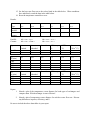
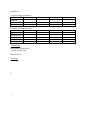
Measurement of Convection Coefficient
Theory
A metal block transferred from a high temperature to low temperature fluid environment will cool
to the new ambient temperature according to the exponential step-response time function. This function
is characterized by a time constant (τ). the time constant is a function of thermal resistance and thermal
capacity. The primary resistance to cooling for this system is a function of convection at the metal-fluid
interface. The thermal capacity of this system is provided by blocks mass having a specific heat value.
τ = RC
R = 1/(hcA)
C = mcp
Objective
Calculate the convection coefficient for an aluminum block in air by determining the system time
constant.
Materials
You will be given an aluminum block, a ruler, and a thermometer. A clock or stopwatch will also
be needed.
Procedure
First, note the room temperature (T∞). Sketch the block and take dimensions. The aluminum
block will be pre-heated to 40 – 60°C. Immediately upon removing the block from the heat source,
contact the thermometer to the block. When the thermometer temperature indicates with the block, start
taking temperature measurements. (Do not just lean the thermometer against the block; make sure there
is good contact.) Measurement intervals should start at 15 seconds; later they may be 30 or 60 seconds.
Monitor temperature until the cooling is at least 75% completed.
Report
Turn in a sketch of the block with its dimensions. Turn in all data, including a plot of ln(T – T∞)
versus time, and all calculations, including time constant and convection coefficient. Briefly comment on
whether or not the convection coefficient seems reasonable.
Specific heat of aluminum: 900 (N m)/(kg °C)
Density of aluminum:
Sketch of block:
T∞:
Table1. Data table.
time (sec)
temperature (°C)
T – T∞
ln(T – T∞)
Concentric Tube Heat Exchanger
Theory:
A heat exchanger is used when it is necessary to transfer heat from one fluid to another without
mixing the fluids. Two types of heat exchangers, parallel flow and counter flow, will be
examined in this lab. The parallel flow heat exchanger has the hot and cold fluids flowing in the
same direction whereas the two fluids flow in the opposite direction with a counter flow
exchanger. The effect of flow rate variation on the performance characteristics of a counter flow
heat exchanger will be studied also.
Heat power emitted = QHρHcpH(tHin - tHout)
Heat power absorbed = QCρCcpC(tCin - tCout)
Heat power lost = heat power emitted - heat power absorbed
Efficiency = (heat power absorbed / heat power emitted) * 100
LMTD = (Δθ1 - Δθ2)/ln(Δθ1/Δθ2)
overall heat transfer coefficient U = Heat power absorbed / (heat transmission area * LMTD)
Objectives:
1. To demonstrate the working principles of a concentric tube heat exchanger operating
under parallel flow conditions.
2. To demonstrate the working principles of a concentric tube heat exchanger operating
under counter flow conditions.
3. To compare the heat transfer characteristics of parallel and counter flow heat
exchangers.
4. To examine the effect of flow rate variation on the performance characteristics of a
heat exchanger.
Procedure:
1.
2.
3.
4.
5.
6.
7.
8.
9.
10.
11.
12.
13.
14.
Close the hot water and cold water flow control valves.
Turn on cold water supply.
Set the selector switch on the side of the pump motor to the maximum setting.
Set the temperature controller to zero using the decade switches on the front panel.
Set the heat exchanger up for parallel flow conditions (see the chart on the front
panel).
Set the electrical supply switch on the ON position and observe operation of the
pump. The top red light on the temperature controller should be illuminated.
Set the temperature controller to 60°C.
Open the hot water control valve and set the flow at 2000 cc/min.
Open the cold water control valve and set the flow at 1000 cc/min.
After conditions have stabilized, record the data in the table below.
After data has been recorded, close the hot and cold water valves and turn off the
power.
Set the heat exchanger up for counter flow conditions (see the chart on the front
panel).
Repeat steps 6 - 11.
Increase the cold water flow rate to 2000 cc/min.
15. Set the hot water flow rate to the values listed in the table below. When conditions
have stabilized, record the data in the table below.
16. Reset the temperature controller to zero.
Results:
Type
tHin
tHmid
tHout
tCin
tCmid
tCout
parallel
counter
Parallel:
Counter:
Δθ1 = tHin – tCin=
Δθ1 = tHin – tCout =
Δθ2 = tHout – tCout =
Δθ2 = tHout – tCin =
Type
Power
Emitted
Power
Absorbed
Power Lost
Efficiency
%
LMTD
(°C)
U
(W/m2 °C)
QH
(cc/min)
1000
2000
3000
4000
tHin
tHmid
tHout
tCin
tCmid
tCout
QH
(cc/min)
1000
2000
3000
4000
Power
Emitted
Power
Absorbed
Power Lost
Efficiency
%
LMTD
(°C)
U
(W/m2 °C)
Parallel
Counter
Report:
1.
Sketch a plot of the temperature versus distance for both types of exchangers and
compare them. Which exchanger is more efficient?
2.
Sketch a plot of temperature versus distance for each hot water flow rate. Discuss
any differences in power, efficiency, and U.
Be sure to include the above data tables in your report
Psychrometrics Lab
ENBE 454
Psychrometrics is the study of the physical and thermal properties of air – water vapor
mixtures. A psychrometric chart relates the properties of dry bulb temperature, wet bulb
temperature, relative humidity, enthalpy, humidity ratio, and specific volume. If any two
properties are known, the others can be determined.
A sling psychrometer may be used to take the dry and wet bulb temperatures. The dry
bulb temperature is independent of the air moisture whereas the wet bulb temperature is
dependent on the moisture content. A sling psychrometer has two thermometers. One
thermometer has its bulb exposed to air. This thermometer is used to measure dry bulb
temperature. The other thermometer has a wetted wick “sock” around its bulb and is used to
measure the wet bulb temperature. The sling psychrometer is spun around in the air at a near
constant velocity.
Objectives:
1. To use a sling psychrometer to measure wet and dry bulb temperatures and relative
humidity inside and outside the building.
2. To use the psychrometric chart to determine relative humidity, humidity ratio, dew
point temperature, constant volume, and enthalpy for the two environments.
3. To determine the mass of dry air in the inside area.
Equipment:
Sling psychrometer
Distilled water
Psychrometric chart
Procedure:
1.
Saturate the wick of the sling psychrometer thoroughly with distilled water (DO NOT USE TAP WATER).
Fill the end cap with distilled water.
In each of the environments:
2.
3.
4.
5.
Pull the end cap to separate the thermometer body from the tube.
Whirl the thermometer body at 2-3 revolutions per second for approximately 1.5 minutes.
Immediately read and record the wet bulb temperature and then the dry bulb.
Slide the body back into the tube until the wet and dry bulb temperatures are opposite each
other.
6. Read and record the percent humidity at the arrow head.
7. Repeat twice in each area.
8. Estimate and record the dimensions of the enclosed area.
9. Use the psychrometric chart to determine the relative humidity, humidity ratio, constant
volume, dew point temperature, and enthalpy.
10. Determine the mass of dry air in the inside area.
Questions:
1.
2.
3.
How does the sling psychrometer relative humidity reading compare with the psychrometric
chart reading?
A stream of air at 1 atm, 18°C, and relative humidity of 70% has a mass flow rate of 0.05
kg/s. A second stream of air at 1 atm, 35°C, and relative humidity of 40% is mixed
adiabatically with the first stream to give a mixed stream temperature of 27°C. What mass
flow rate of the second stream is required? What is the relative humidity of the mixed
stream?
Desert air at 36°C with 25% relative humidity is passed through a swamp cooler, a device
that contacts the dry air with a wet surface. Water in the swamp cooler is evaporated until
the desert air is saturated with water vapor. The swamp cooler is assumed to operate
adiabatically, and the water in the swamp cooler is at the temperature of the air leaving the
swamp cooler. What will be the temperature of the saturated air leaving the swamp cooler?
TURN IN THE DATA SHEET AND YOUR THREE PSYCHROMETRIC CHARTS AT
THE END OF THE LAB PERIOD.
Data Sheet
Using the sling psychrometer:
Inside
Wet bulb
Dry bulb
RH
Using the psychrometric chart:
Inside
RH
Humidity ratio
Dew point
Enthalpy
Constant vol.
Calculations:
Dimensions of inside area:
Volume of inside area:
Mass of dry air:
Questions:
1.
2.
3.
Outside
Outside
PUMP LAB
THEORY
A driving force is needed to move a fluid from one point to another. The driving force may be
supplied by gravity or by a mechanical device such as a pump or fan. Generally, the word
“pump” is used to describe a device that moves an incompressible liquid. Fans, blowers, and
compressors are devices used to move gases. In pumps and fans, the density of the fluid does not
change appreciably, and incompressible flow can be assumed. In this lab, we will be looking at
the operation of centrifugal, piston, gear, rotary, booster, screw, and roller pumps.
OBJECTIVES
1. To learn the operational characteristics of different pumps.
2. To determine the characteristic curves for a pump.
MATERIALS
one each PUMP TEST STATION
one each PUMP TEST STATION Operating Instructions, Maintenance and Parts Manuals
PROCEDURES
Examine the operation of centrifugal and booster pumps (Pump Station A), and gear, piston,
screw, and roller pumps (Pump Station B). Follow the manual for the correct operation of the
pumps. Operate the pump at a constant speed over a range of flow rates. Obtain and record the
following measurements: pressure, flow, speed, and power. Notice the difference between the
characteristic curves of the pumps.
REPORT
Graph a pressure versus flow curve for each pump. Briefly discuss the relationship between
pressure and flow for each pump. Be sure to include the data. You can place all the graphs and
tables onto one page, as long as they are still legible.
Pump type:
Pressure (psi)
Pump type:
Pressure (psi)
Pump type:
Pressure (psi)
Speed:
Flow (gpm)
Power (W)
Speed:
Flow (gpm)
Power (W)
Speed:
Flow (gpm)
Power (W)
Pump type:
Pressure (psi)
Pump type:
Pressure (psi)
Pump type:
Pressure (psi)
Speed:
Flow (gpm)
Power (W)
Speed:
Flow (gpm)
Power (W)
Speed:
Flow (gpm)
Power (W)
Pump type:
Pressure (psi)
Speed:
Flow (gpm)
Power (W)
Reverse Osmosis Laboratory
Summary of Theory
A reverse osmosis membrane is a polymer film in which, for various physicchemical reasons, water dissolves much more readily than solutes. The water then
diffuses through the membrane under a chemical potential gradient. Dissolving a solute
in water reduces the chemical potential of the water so that if there is pure water on the
other side of the membrane, water will diffuse from the water side through the membrane
into the solution.
One way of increasing the chemical potential of water in a solution is to
pressurize it. The pressure that is required to bring the chemical potential up to that of
pure water, and so stop diffusion through the membrane, is the osmotic pressure. If a
pressure greater than this is applied to the solution, the chemical potential gradient is
reversed and water flows through the membrane form the solution into the water.
Material
- approximately 10 liters of salinated water
- 10 ml measuring cylinder
- stop watch
- salinity refractometer
Equipment Set-up
Set up the equipment for operation in Reverse Osmosis mode as described in the
Operational Procedures. The salt water will be circulating at 18 liters/min and the system
pressure will be 10 bar.
Procedure
First, measure the concentration of salt in the water using the salinity refractometer.
Record this value.
Soon after the operating conditions have been set up, permeate will begin to enter the
permeate tank through the module outlet pipe on the right hand side of the module.
Hold the measuring cylinder beneath the permeate outlet pipe and at the same time start
the stopwatch. Time how long it takes to collect 10 ml of permeate.
Calculate the flow rate of permeate in ml/min and log the value. Measure the salinity of
the water.
Slowly adjust the system pressure using valve V1 to 15 bar. Wait for approximately 2 minutes
for the new process conditions to stabilize. Take a reading of flow rate using the same method as
before and log it. Again, determine the salinity of the water.
Repeat this exercise for system pressure of 20, 25, 30, 35, and 40 bar.
Results
Pressure (bar)
Permeate flow rate (mL/min)
Salinity
5
10
15
20
25
Construct a graph of flow rate versus pressure. This will give a curved line up to a certain
pressure and then the line will straighten and become horizontal. Determine the pressure at
which the line becomes horizontal. Extrapolate the curve to the x-axis and determine the x
intercept. This will be the osmotic pressure of the salt water.
The flattening of the curve at higher pressures is due to concentration polarization. The
plateau is reached when the flow is such that salt approaches the membrane at the same rate at
which it diffuses back into the bulk liquid. Attempts to increase the flux by increasing the
pressure merely increases the thickness of the polarized layer until the same limiting flux is
reached.
Lab Report
Your report should include the data table and the graph. State the osmotic pressure of the
salt water and the pressure at which the curve becomes horizontal.
ENBE 454 Biological Process Engineering
Systems Lab
Theory:
The Test Lung has been developed to simulate the flow of air in the lungs using a simple
model. The lungs can be configured in either a single-lung or dual-lung mode. The lungs are
simulated using bellows. At rest, each bellows contains a volume of air equivalent to the average
adult’s functional residual capacity. Resistances are used to represent the upper airways
resistance and lower airways resistance in each lung while compliance of the lungs is adjusted
using springs.
Changes in the resistance or compliance of the lung due to illness or disease will affect
the performance of the lung. This lab will investigate some of those changes.
Objective:
1. To observe the effects of changing compliance on flow rates in the lungs.
2. To draw a systems diagram representation of the system.
Materials:
1 each, Michigan Instruments Dual Adult TTL, Model 2600i (test lungs)
1 each, 486 IBM compatible PC
1 each, Michigan Instruments software, PneuView DA v2.13
Preliminary Set-Up
Set up the TTL in the DUAL LUNG Simulation configuration (see p. 2-2 of the User’s Manual)
with proximal, left, and right resistances of 5 cmH2O/L/sec. Attach the adaptor/power cord to
the back of the TTL device; plug the other end into the wall socket. Turn on the TTL using the
switch on the back of the device. Connect a cable from the printer port of the computer to the
port on the back of the TTL. Turn on the computer. The program is DOS based and does not
run well from WINDOWS. From the c:\ prompt, change to the pv2 directory (c:\cd pv2). Type
pv to start the program. (Note the TTL must be turned on and connected to the computer via the
printer port before the program is started.) The program is now in the Primary Working
Environment.
WARNING
Do not change the compliance on the TTL while the lungs are being ventilated. Severe
damage may result.
Units used with the system
Pressure: cmH2O
Volume: L
Resistance: cmH2O/L/sec
Compliance: L/cmH2O
Part I
Demonstration of Ventilation Phenomena
In this section, we are going to look at the effect pneumonia has on the distribution of delivered
tidal volume.
Lung Set-up
1. Set the syringe volume to 0.8 L. (Use a hex key to change the stop on the plunger.)
2. Set both lung compliances at 0.05.
3. Move the scale markers at the top of the lungs (near the tidal volume scale) to 0.05 to match
the selected compliance.
4. Fill the syringe with 0.8 L of air and connect the syringe to the lungs.
Computer Set-up
1. From the Primary Working Environment, use the mouse to select the Calibration mode. Press
A for Autosave and then press M or Menu. Press <ENTER> to return to the Primary Working
Environment.
2. Use the mouse to select Acquire Mode.
3. Change the Reference Conditions so that all the resistors have values of 5.
4. Change the Respiratory Parameters to display right and left peak pressures and volumes.
Leave other default parameters selected. (i.e., don’t change anything else!)
5. Change the Waveform Display 1 to show the total volume. Change the x-axis scale to 60
seconds.
6. Change the Waveform Display 2 to show the right and left volumes. Change the color of the
traces. Change the x-axis scale to 60 seconds.
Ventilating the lungs
Ventilate the lungs at a rate of 12 breaths per minute (2.5 seconds for each push/pull of the
plunger). Be sure to use a smooth, steady motion. It will take a few breaths for data to appear on
the screen. Once you have a smooth breathing pattern around 12 breaths per minute, take a look
at the waveform displays and the respiratory parameters. What is the pressure in each lung, the
volume in each lung, and the total tidal volume? Record this information on the data sheet.
Stop ventilating the lungs. Change the compliance of the right lung only to 0.03, then 0.02, and
finally 0.01 and note the lung volumes and pressure with each change. Be sure to change the
compliance values in the Reference Conditions window. Record the information in the table
below.
Shut-down:
Press M for Menu.
Press Q for Quit and press <ENTER> to return to the Primary Working Environment.
Use the mouse to select Exit PneuView and press <ENTER>.
Turn off the monitor, computer, and test lung.
Complete the write-up before leaving the lab.
Making changes when in Acquire mode
Changing Reference Conditions
Using the mouse, click on the C of the Reference Conditions window. Enter the correct
compliance and resistance values. The resistance values are changed by clicking on the box with
the value in it. Defaults are 5 for left and right lung resistance and 20 for proximal resistance.
Click on the 20. The box should now be highlighted. With subsequent clicks, the values will
scroll through the possible values (5, 20, 20). Select the appropriate value. Compliance values
are changed by clicking on the value and typing in the new value. When changes are complete,
click on the OK box. If you do not wish to make changes, or you do not want to save the
changes you made, click on the CANCEL box.
Changing the Respiratory Parameters
Using the mouse, click on the P of the Respiratory Parameters window. Click on the boxes at the
left to select which parameters are displayed. A red square in the box indicates that that
parameter is selected. You can delete a selection by clicking on a box that already has a red
square in it. When changes are complete, click on the OK box. If you do not wish to make
changes, or you do not want to save the changes you made, click on the CANCEL box.
Changing the Waveform Display
There are two Waveform Display windows. Each display may display up to three waveforms.
Using the mouse, click on the 1 or the 2 of the Waveform Display window you wish to change.
Waveforms are selected by clicking on the boxes at the left. Ranges for the y-axis may be
changed for each variable by clicking on the box and entering a new value. The x-axis for the
graph may be changed in the same way. If you are displaying two or more waveforms on one
display, be sure to change the color of at least one of the traces. The color is changed by clicking
on the colored box at the right of the selected waveform. Subsequent clicks on the box will cycle
through the available colors. Only certain color combinations are permitted, so you will see
different color choices for the current trace depending on the color selected for the other trace(s).
When changes are complete, click on the OK box. If you do not wish to make changes, or you
do not want to save the changes you made, click on the CANCEL box.
Notes Window
A description of the demonstration may be entered in the Notes window. Using the mouse, click
on the N of Notes. Type whatever you wish. When changes are complete, click on the OK box.
If you do not want to make changes, or you do not want to save the changes you made, click on
the CANCEL box.
ENBE 454 Biological Process Engineering
Systems Lab Data Sheet
Respiration rate: ______________
Proximal resistance: ____________
RR
CR
5
RL
CL
0.05
5
0.05
5
0.03
5
0.05
5
0.02
5
0.05
5
0.01
5
0.05
Table 2. Data
VR
PR
VL
PL
Vtotal
ENBE 454 Biological Process Engineering
Systems Lab Write-Up
1. Draw a systems diagram for the lung setup. Be sure to label each component.
2. Explain (in 25 words or less) the changes you saw.
3. Pneumonia is classified as a restrictive disease. Bronchitis, asthma, and emphysema are considered obstructive
diseases. What changes in respiration (particularly resistance) would you expect to see in someone with bronchitis?
4. Where would you expect to find inertance in the test lungs?
5. What is wrong with the table on the data sheet if that table were to appear in a technical document (list at least
three)?
Each student should turn in a copy of the Data Sheet and Write-Up at the end of the lab.
ENBE 454
Viscosity Lab
THEORY
Viscosity
Viscosity is the measure of the internal friction of a fluid. This friction becomes apparent when a
layer of fluid is made to move in relation to another layer. The greater the friction, the greater the amount
of force required to cause this movement, which is called “shear.” Shearing occurs whenever the fluid is
physically moved or distributed, as in pouring, spreading, spraying, mixing, etc.
Fluids are classified into two types depending on their flow behavior. Newtonian fluids have a
straight line relationship between shear stress and shear rate. A typical Newtonian fluid is water. Most
fluids fall into the other category, the non-Newtonian fluids. Non-Newtonian fluids are classified by the
way that fluid’s viscosity changes in response to variation in shear rate. Pseudoplastics have a decreasing
viscosity with an increasing shear rate. Examples include paints and emulsions. Dilatant fluids have
increasing viscosity with an increasing shear rate. Clay slurries, candy compounds, and sand/water
mixtures are all dilatant fluids. A fluid that behaves as a solid under static conditions but then flows after
a certain amount of force has been applied is a plastic. Cheese is a good example of this type of fluid.
Viscometer
The viscometer that will be used in this laboratory is a rotational viscometer. It measures the
torque required to rotate an immersed spindle in a fluid. The spindle is driven by a synchronous motor
through a calibrated spring. For a given viscosity, the viscous drag, or resistance to flow (indicated by the
degree to which the spring winds up), is proportional to the spindle’s speed of rotation and is related to
the spindle’s size and shape (geometry). The drag will increase as the spindle size and/or rotational speed
increase. It follows that for a given spindle geometry and speed, an increase in viscosity will be indicated
by an increase in the deflection of the spring.
OBJECTIVES
1. To learn to operate a rotational viscometer.
2. To determine to the viscosity of fluids using a rotational viscometer.
3. To determine the composition (v:v) of fluid using a standard curve of viscosity versus
composition.
MATERIALS
one each Brookfield DV-II+ rotational viscometer
one each 600 mL beakers
two each mixture of unknown composition
four each mixture of known composition (0%, 15%, 30%, 45%)
PROCEDURE
1.
2.
3.
4.
Level the viscometer.
Turn on the viscometer.
Press any key to autozero the viscometer.
Put spindle one onto the viscometer: Push up on the screw attached to the viscometer and
screw on the spindle. (The spindle has left-handed threads.)
5. Press any key to continue.
6. Press the SET SPEED button. Press the up arrow so that the speed is set to 100 rpm.
7. Press the MOTOR ON/OFF button.
8. Press the SELECT DISPLAY button until the units are mPas.
For each sample:
1. Pour the contents of one of the bottles into the 600 mL beaker. Add 200 mL of water.
2. Using the stirring rod, stir the mixture until it is no longer cloudy.
3. Lower the viscometer into the fluid until the notch on the spindle shaft is just below the fluid
surface.
4. Press the MOTOR ON button.
5. Wait until the reading is steady and then read the display. Record the concentration and
viscosity in the table below.
6. Press the MOTOR OFF button.
7. Raise the spindle until the viscometer clears the top of the beaker.
8. Pour the contents of the beaker into the sink and rinse the beaker.
9. Repeat above steps until you have measure the viscosity of all four samples and the two
unknowns. Be sure to record which unknowns you are testing.
Concentration
Viscometer Reading
Unknown:
Unknown:
REPORT
Using Excel or another spreadsheet,
1) create a table of the viscosities and compositions;
2) plot the viscosity versus composition.
Indicate on the plot the viscosity of the unknown fluid and whether it is unknown A, B, C, or D. Estimate
the composition of the unknown fluid using the plot. (Don't just indicate it on the graph; state it.)
Turn in the table, plot, and your estimate of the composition of the unknown by 2:00 P.M. on the day of
your next recitation. Be sure that you properly label your table and plot. Each student is expected to turn
in a separate report.