Download Deriving a geometrical characterization of an arteriovenous fistula

Deriving a geometrical
characterization of an
arteriovenous fistula for mesh
creation and CFD simulation
Lars W. J. Pustjens
BMTE 11.20
Deriving a geometrical characterization of an arteriovenous fistula
for mesh creation and CFD simulation
Lars W. J. Pustjens
Department of Biomedical Engineering, Eindhoven University of Technology
Student number:
Internship period:
Institute:
Coaches:
Supervisor:
0567568
From 22-3-2011 till 5-7-2011
Maastricht University
Dr. Ir. Mariëlle Bosboom & Maarten Merkx MSc
Prof. Dr. Ir. Frans van de Vosse
2
Table of Contents
Abstract ...................................................................................................................................................... 5
1. Introduction ............................................................................................................................................ 7
2. Materials and Methods ........................................................................................................................... 9
2.1 Patient data....................................................................................................................................... 9
2.2 AVF Segmentation............................................................................................................................. 9
2.3 AVF Fitting ....................................................................................................................................... 10
2.4 Mesh Creation & CFD ...................................................................................................................... 12
3. Results................................................................................................................................................... 15
3.1 AVF Segmentation........................................................................................................................... 15
3.2 AVF Fitting ....................................................................................................................................... 16
3.3 Mesh Creation & CFD ...................................................................................................................... 18
4. Discussion & Conclusion ....................................................................................................................... 21
4.1 AVF Segmentation........................................................................................................................... 21
4.2 AVF Fitting ....................................................................................................................................... 21
4.3 Mesh creation & CFD ...................................................................................................................... 21
4.4 Conclusion & Recommendations .................................................................................................... 22
Acknowledgments .................................................................................................................................... 23
Bibliography .............................................................................................................................................. 25
Appendix ................................................................................................................................................... 27
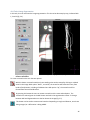
Appendix A: User Manual LabVAS ........................................................................................................ 27
Appendix B: Patient-specific fitting results ........................................................................................... 40
3
4
Abstract
Patients suffering from End-Stage Renal Disease (ESRD) are treated with a renal replacement therapy,
e.g. hemodialysis. For hemodialysis, a vascular access (VA) is needed to connect the artificial kidney to
the patient. The preferred VA is the arteriovenous fistula (AVF), which is created by connecting a vein to
an artery to increase the blood supply (> 300 ml/min) to the hemodialyzer. Unfortunately, 30%-50% of
the fistulas will encounter complications and pre-surgical examinations are thus needed. The aim of the
ARCH project is to develop a patient-specific model to aid in pre-surgical decision making. In this model
the vascular network is described by 1D wave propagation segments, which are terminated by 0D
windkessels. However by using this 0D/1D description, the hemodynamics in the AVF, i.e. the extra
pressure drop in the arterial-venous connection resulting from secondary flow, is not currently
described. To model these, a 3D AVF geometry and 3D computational fluid dynamics (CFD) simulations
are required. These 3D simulations can be used to derive a pressure/flow relation for the AVF that can
be implemented in the 0D/1D model. In previous research a generic AVF geometry was used in the 3D
CFD simulations, but this geometry was not based on patient data. The aim of this project is to derive a
geometrical characterization of an AVF, based on patient data, and to use this characterization for mesh
creation and 3D CFD simulations.
Post-surgical CE-MRA data of 12 AVF patients, examined 6 weeks after surgery, is used. The AVF’s are
segmented, using the LabVAS prototype. LabVAS segments the AVF’s by extracting the centerline
coordinates, using a wave propagation technique, and by extracting the vessel contour, using an edge
detection algorithm. The geometries, obtained with the segmentation, are fitted with earlier proposed
centerline and diameter functions, by using a nonlinear least squares fitting method, based on the Trust
Region algorithm. In this way, geometrical functions are obtained based on patient data. By averaging
the parameters of these fitted functions, a characterization is obtained for a radiocephalic AVF (RC-AVF)
and a brachiocephalic AVF (BC-AVF). These characterizations are used to create two meshes with the
Vascular Modeling ToolKit (VMTK). Hereafter, 3D CFD simulations are performed to evaluate the flow
and pressure distributions due to the anastomosis.
The most important differences between the generic geometries and the patient-based geometries are
the arterial and venous diameters, which were previously chosen too small and the parameters
describing the angle of the anastomosis, which previously could vary over a too large range. Due to
these differences the pressure drop over the anastomosis will be lower than previously expected.
5
6
1. Introduction
In Europe, more than half a million people suffer from severe chronic kidney disease, e.g. end-stage
renal disease (ESRD). ESRD corresponds to the loss of the kidneys’ ability to eliminate excess fluid and
waste material from the blood. Due to a shortage of donor kidneys, the majority of ESRD-patients (69%)
are treated by renal replacement therapy, e.g. hemodialysis. The success of the hemodialysis treatment
is related to the success of the vascular access (VA) surgery. The VA is created to connect the patient’s
blood circulation to the artificial kidney. There are three types of VA: arteriovenous fistula (AVF),
arteriovenous graft (AVG) or central venous catheter (CVC). Due to its long-term performance, when
compared to AVG and CVC, AVF is the first choice of VA (1).
In the AVF, a vein is surgically connected with an artery to create an anastomosis. The low resistant
anastomosis results in a high blood flow between the feeding artery and draining vein, which is needed
for efficient dialysis. To enable hemodialysis, the flow through the extracorpeal artificial kidney must be
at least 300 ml/min (2). Normally the radial artery has a flow of about 20-30 ml/min. Directly after AVFcreation (artery side-to-vein end) the flow increases up to 200-300 ml/min. After maturation, the AVF
flow rate will reach 600-1200 ml/min, which is sufficient for hemodialysis (3). This increase in flow is a
result of both vascular dilatation and remodeling.
Throughout history three kinds of AVF’s have been evaluated. The first was the side-to-side AVF, second,
the end-to-end AVF and third, the side-to-end AVF. All three techniques have advantages and
disadvantages. The side-to-side anastomosis has the advantage of technical simplicity but has the risk of
venous hypertension, with swelling of the hand. The end-to-end anastomosis has the advantage of a
limited fistula flow, but is technically more demanding, due to difference in diameter of vein and artery,
and could lead to ischemia of the hand. Nowadays, the commonly used technique is the side-to-end
anastomosis. This technique will anastomose the vessels, without creating an acute angle. To create the
anastomosis, the surgeon must make an incision in the artery wall, a so called arteriotomy. The length of
this arteriotomy is guided by the angle that will be achieved when connecting the vein to the artery
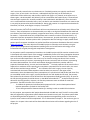
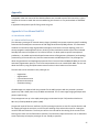
(figure 1.1) (4).
Figure 1.1: When the vein (V) is connected to the artery (A) the
length of the arteriotomy could differ when a different angle is
(3)
used .
Figure 1.2: Seven segment AVF circuit: (1) proximal artery,
(2) distal artery, (3) arterial collaterals, (4) proximal vein,
(5) distal vein, (6) venous collaterals and (7) the
(5)
arteriovenous anastomosis (here radiocephalic) .
7
AVF’s are usually created in the non-dominant arm. Two body locations are typically used for AVF
surgery. First, at wrist level in the forearm, a radiocephalic AVF (RC-AVF) can be formed by an
anastomosis of the radial artery and the lower cephalic vein (figure 1.2). Second, at the upper arm, or
elbow region, a brachiocephalic AVF (BC-AVF) can be created when the brachial artery is anastomosed
with the upper cephalic vein. Another possibility is the brachiobasilic AVF (BB-AVF), where the basilic
vein is connected with the brachial artery. Here, the basilic vein should be relocated in such manner that
it can easily be punctured to perform hemodialyis. During AVF-creation it is important that obstacles for
blood flow, like kinks, acute angles or torque, are avoided (1) (4).
After AVF creation, 30%-50% of the RC-fistula will have complications that will lead to early failure of the
fistula (6). These complications are characterized by a too low or too high AVF blood flow and could lead
to ischemia of the hand (steal syndrome), congestive heart failure, central venous stenosis or aneurysm
formation (4). To decrease these early complications and increase the number of functional AVF’s, it is
important to perform preoperative examinations, like anamnesis, physical examination or imaging of
arm arteries and veins. Another option to aid in preoperative decision making is to apply model-based
patient-specific computer simulations to predict blood flow and pressure distribution after AVF creation
(www.vph-arch.eu). The main objective of the ARCH project is to develop such simulator, using the
patient-specific image-based computational modeling tools and an information technology service
infrastructure for surgical planning and complications management.
For the patient-specific computational simulations in the ARCH project a 0D/1D vascular network solver
is developed, where each branch of the network is modeled by means of 1D wave propagation elements
and terminated by a 0D windkessel element (7) (8). By assuming viscous dominated flow in the boundary
layer and inertia dominated flow in the vessel core, an electrical analog was derived. Each vascular
element now consists of a resistor, representing the viscous resistance, and an inductor, representing
the inertia dominated flow. The resistor and inductor depend on Womersley number and local
properties like blood density, viscosity and vessel diameter (9). The local properties of the vessel wall are
captured in a conductor which represents the compliance computed from the vessel radius, the vessel
wall thickness and the Youngs modulus (10). For simulation of the AVF surgery, the non-linearity
associated with the Navier-Stokes equations must be taken into account in the region of the
anastomosis, where the Womersley theory assumptions of a cylindrical wall and parallel and linear flow,
are considered invalid. In this region, a special element for the AVF should thus be used. The pressureflow relation for this element can be derived from 3D Computational Fluid Dynamics (CFD). As input for
the CFD the AVF geometry should be known. In the ARCH Deliverable D5.3 (11), analytical functions were
derived for the AVF geometry. However, the function parameters were not based on actual AVF
geometries. Therefore the aims of this report are:
- To validate the geometrical characterization proposed in D5.3, and to obtain patient-based
equation parameters for both RC-AVF and BC-AVF
- To use these geometrical characterizations for meshing in order to enable CFD simulations.
For this purpose, post-operative AVF patient data obtained with MRI are used. The AVF’s on these MRI
data are segmented, to get patient-specific blood vessel centerlines and radii. The patient-specific data
are fitted with geometrical equations (11). And, the population-averaged fitting results are used as an
input for mesh creation and CFD computations. This is all described in chapter 2. The results are given in
chapter 3. In chapter 4 the results will be discussed and conclusions will be drawn regarding the aim of
the project.
8
2. Materials and Methods
In the first section of this chapter, 2.1, information is given about the patient datasets used in this
research. In the second section, 2.2, the AVF segmentation technique is described. In the third section,
2.3, the fitting procedure to extract a population-averaged description of the AVF geometry is explained.
In the last section, 2.4, the process of mesh creation and CFD simulation is described.
2.1 Patient data
To obtain a characterization of the AVF-geometry, post-surgical patient data, gathered six weeks after
AVF creation, was used. The data contains information about side-to-end AVF’s, both radiocephalic and
brachiocephalic. The patient data was acquired with the ARCH-protocol (12). In this protocol a proximal
(upper arm) and a distal (lower arm) Contrast Enhanced Magnetic Resonance Angiography (CE-MRA)
were obtained, using a two-stage imaging technique with patient repositioning.
The original population contained 17 patients. Due to the lack of a CE-MRA dataset five patients were
excluded. In the remaining twelve datasets, there were six patients with a RC-AVF and six patients with a
BC-AVF. Post-surgical CE-MRA data describing a BB-AVF was not available.
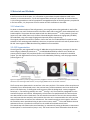
2.2 AVF Segmentation
The AVF geometry was segmented from the CE-MRA data using the Laboratory prototype for Vascular
Access Surgery (LabVAS) (by Merkx et al. (12)), an ARCH dedicated Philips software tool. LabVAS can
process proximal (upper arm) and distal (lower arm) CE-MRA datasets as are acquired in the ARCH
project. The AVF segmentation of artery and vein was obtained by following a two-step segmentation
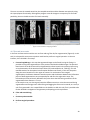
process (figure 2.1).
Figure 2.1: Segmentation process by using (a) the wave propagation method for centerline extraction (example of arterial side),
with the arrows indicating the flow direction, and by using (b) FWHM-criterion for diameter extraction.
The first step was to determine the centerlines in the artery and vein. The creation of the centerline was
initiated by a user-defined seed point in the proximal artery of the anastomosis and a user-defined end
point in the distal artery. To distinguish vessel structures from the background, a wave propagation
technique, i.e. fast marching method, was used (13) (see fig. 2.1a). The wavefront propagated from the
seed and end point until collision. Subsequently, the minimum cost path between start and end point
was determined from the visited voxels. For the centerline extraction of the vein the same procedure
was used, now with the seed point at the position where the vein is anastomosed to the artery and the
end point behind the curvature of the anastomosis. The created centerlines were irregular; therefore
the centerlines were repositioned using an open active contour model (14). This model balances internal
and external forces, to position the centerline in the middle of the blood vessels lumen.
The second step was to detect the vessel boundary, by automatically setting up diameter measurement
location points on each centerline (every 1 mm). The vessel contours were extracted at these discrete
9
points, using an edge detection algorithm. For the edge detection, twenty radial rays were casted
perpendicular to the local vessel direction, at every measurement location point. Hereafter, the local
vessel contour was extracted by applying the Full-Width at Half-Maximum (FWHM) criterion (fig. 2.1b).
For calculating the radius of the blood vessel LabVAS first calculated the cross sectional area (A) found
with the FWHM method. With this cross sectional area the local diameter (d) is determined using the
equation:
During the segmentation steps the results are inspected for verification and, in case of disagreement,
altered by changing or deleting centerline or vessel boundary points.
After finishing the segmentation process, geometrical data is available for further evaluation. The
geometrical data contains vessel wall coordinates at discrete points of the vessel centerline and the local
measurements of radii in the vein and arteries.
A detailed description of the segmentation procedure can be found in the article of Merkx et al. (12) or in
the first chapter of the LabVAS user manual (Appendix A1). A detailed user instruction of LabVAS is
described in the second chapter of the user manual (Appendix A2).
2.3 AVF Fitting
With the geometric descriptions, obtained using the LabVAS segmentation on the CE-MRA datasets, it is
possible to determine parameterized functions of the centerlines and to evaluate the change in
diameter of the anastomosis. In the ARCH Deliverable D5.3 (11) equations have been proposed describing
the centerlines and radii of the arteries, proximal and distal, and the vein (eq. 2.2). By combinations of
parameter a and b, the angle of the anastomosis is described. In ARCH Deliverable D5.3 these
parameters are chosen, with a = 1 or 1.5 and b = 0.2, 0.5, 1.0 or 1.5, to cover a wide range of angles. The
diameters of artery (dart) and vein (dv) are chosen, with dart = 2 and dv = 2, 3 or 4, to obtain a dv/dart ratio
of 1, 1.5 and 2. For CFD modeling the vein is tapered and the artery is slightly curved in order to break
the symmetry. Using equations 2.2 will lead to a generic representation of an AVF (see fig. 2.2).
Equations 2.2: Equations used in ARCH Deliverable D 5.3
Artery Proximal (ap)
Artery Distal (ad)
Vein (v)
With s = [0,1] with s=0 at site anastomosis, dart=2mm, dv={2,3,4}mm and (a,b) = {(1,0.2), (1,0.5), (1,1.5), (1.5,1.5)}. Here s* is
used to define the region in which the vein is tapered.
10
Figure 2.2: Generic AVF geometries using equations 2.2 with dv = dart = 2 mm and a = 1.5 and b = 1.5 (top) and a = 1 and b = 0.2
(bottom), no tapering so s* is neglected.
These equations were also used for fitting the patient data. First a few preprocessing steps were
performed. The LabVAS data was imported into mathematical software (MatLab, the MathWorks Inc.)
and the coordinates of the data were adapted so that the anastomosis of artery and vein is in the origin,
(x,y,z)=(0,0,0), of the image. Next, the data was rotated to locate the distal artery on the x-axis and the
vein in the positive z-direction in order to satisfy the criteria of yap=0, yad=0 and zad=0 (see figure 2.3).
Figure 2.3: Rotation of the centerlines; dotted line is the original position of
the data, the full line is the rotated position;
data of patient 20008
11
Further, to fit the centerlines and radii of the patient datasets with the proposed equations (eq. 2.2), the
functions had to be altered. From quick data review it was concluded that:
- The length of arteries and veins is not the same; this is solved by using a length-factor c as
parameter in the equations, that replaces the fixed lengths in xap, zap, xad, xv , yv and zv.
- To make the equations independent of the diameter, dart =2 is chosen.
- Change of centerline position in x-direction is not always linear; sb is chosen instead of s1 in xap,
xad and xv.
- Change of centerline position in z-direction is not always quadratic; sb is chosen instead of s2 in
zap and zv.
- The diameters of the artery and vein hardly change over the length, so dap, dad and dv are
constant and fitted on the data.
This resulted in the following equations (eq. 2.3):
Equations 2.3: Fitting equations
Artery Proximal (ap)
Artery Distal (ad)
Vein (v)
These twelve equations (eq. 2.3) are individually fitted with the patient data, using a nonlinear least
squares fitting method, based on the Trust-Region algorithm (15). After fitting, the parameters of the RCAVF and of the BC-AVF were averaged to create characterizations for both RC-AVF and BC-AVF. These
AVF configurations will be modeled separately because they differ in arterial and venous diameters and
in angle of the anastomosis.
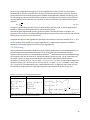
2.4 Mesh Creation & CFD
To use the characterization of the RC-AVF and BC-AVF for creating a mesh, the centerlines and
diameters were converted to a VTK (www.vtk.org) compliant format (with use of Python, from
Enthought). Afterwards, the vessel surfaces, defining the anastomosis model, were generated using the
Vascular Modeling ToolKit (VMTK, www.vmtk.org). For the complete procedure on how to use VMTK,
see the ARCH deliverable D5.3 (11). In short, VMTK uses the centerlines and radii to obtain a digital
segmented image. This image needs automatic clipping and smoothing to obtain flat surfaces at the
inflow and outflow regions and a smooth intersection at the bifurcation. After this the mesh can be
generated.
For CFD, the flow in the arteries and vein had to be fully developed. Therefore the venous and arterial
lengths were enlarged with a straight tube. The number of mesh-elements was chosen in the range of
150000 and 200000 elements. This was achieved by iteratively changing the edgelengthfactor by trial
and error until the proper range was reached. In VMTK the edgelengthfactor is defined as the absolute
nominal length of a surface triangle edge.
As final step, the created mesh was evaluated by means of 3D CFD computations. In the CFD
computation incompressible Navier-Stokes equations are solved for a constant inflow. By defining a
Reynolds number the inflow was calculated via:
12
In this equation
is defined as the mean velocity at the proximal artery and as the blood density
with value
and as the dynamic viscosity with value
. As a result of high
pressure in the proximal artery and low pressure in the vein, flow will distribute from artery to vein. In
this research 90% of the flow rate, in a RC-AVF, and 80% of the flow rate, in a BC-AVF, goes via the
anastomosis through the vein. By use of fully developed Dirichlet boundary conditions at the inflow of
the proximal artery and at the outflow of the distal artery these flow rates can be imposed. The
simulations were performed with the open-source hemodynamic solver Gnuid (available from
github.com/lorbot/Gnuid) which uses the incompressible Navier-Stokes solver implementation of Botti
et al. (16) (also see ARCH Deliverable D5.3 (11)). After CFD simulation, the results were evaluated using a
visualization application (Paraview, from Kitware). With use of this application flow streamlines are
generated, and the pressure drop is determined. Here, the pressure drop is defined as the difference in
pressure between the proximal artery and the vein.
13
14
3. Results
This chapter shows the results of the segmentation (3.1), the fitting of the patient data (3.2) and the
results of mesh creation and CFD modeling (3.3).
3.1 AVF Segmentation
With LabVAS segmentations of the AVF geometries could be made for all CE-MRA datasets. Two
examples are shown in figure 3.1.
a. Segmentation of p20005; RC-AVF
b. Segmentation of p20008; BC-AVF
Figure 3.1: Examples of segmentations; The crosses are the starting point; Seed 1 is
located in the vein and Seed 2 in the artery
Segmentation resulted in a dataset containing: (a) the vessel wall coordinates, (b) the centerlinecoordinates and (c) the radii of the artery and vein (figure 3.2).
c. Vessel wall coordinates
d. Centerline-coordinates
e. Radii of artery and vein
Figure 3.2: Results of the segmentation, note that the ring-coordinates and the centerline coordinates differ, here red = artery,
blue = vein; the increase in the radius of the artery is a result of an segmentation error at the site of the anastomosis, as is the
increase in radius at the beginning of the vein; data of p20005
In figure 3.2a it can be seen that at the position of the anastomosis the artery and vein overlap. This will
result in an increased radius for both artery and vein at the position of the anastomosis, as can be seen
in figure 3.2c. In figure 3.2b it can be noted that the artery is slightly curved towards the vein, which is a
result of lifting the artery during surgery.
15
3.2 AVF Fitting
Using a nonlinear least squares fitting method of the AVF equations on the patient geometry, results in a
patient specific geometrical characteriazation of the anastomosis (figure 3.3). For all AVF geometries,
fitting of the centerlines, using the proposed equations gave good results. In table 3.1 an overview of
the fitting results is given. In this overview the median as well as the range of the parameters are given
for both RC-AVF and BC-AVF. In this table also a comparison is made with the parameters previous
chosen for the generic AVF described in Deliverable D5.3 (11). For the results per patient, see appendix B.
Table 3.1: overview of the fit-parameters; For the RC-AVF and the BC-AVF, the median value of each parameter
and the total range of the parameter, between brackets, are given.
Range of parameters
Parameter
xap
zap
RC-AVF
BC-AVF
c
11.5 (9.8, 14.1)
11.8 (5.6, 20.3)
15
b
1.0 (0.99, 1.4)
0.99 (0.98, 1.4)
1
Parameter well chosen in D5.3
c
-1.2 (-5.5, 4.2)
-0.38 (-9.8, 9.9)
1
Parameter determines length proximal artery in z
b
0.9 (0.17, 1.2)
1.1 (1.0, 1.2)
2
Parameter is smaller than in D5.3
4.15 (3.2, 5.0)
5.1 (3.8, 6.5)
2
Parameter is larger than in D5.3
c
-6.6 (-11.6, -4.9)
-6.8 (-15.4, -2.9)
b
0.99 (0.97, 1.3)
1.0 (1.0, 1.1)
1
Parameter well chosen in D5.3
3.9 (3.9, 5.6)
4.5 (3.4, 5.7)
2
Parameter is larger than in D5.3
c
11.4 (8.7, 15.8)
8.2 (4.9, 15.8)
15
b
1.0 (0.83, 1.2)
1.4 (0.88, 1.7)
1
c
9.9 (8.7, 14.1)
11.2 (7.1, 28)
15
a
0.86 (0.73, 0.87)
0.93 (0.39, 1.1)
(1, 1.5)
b
1.75 (0.79, 3.2)
0.89 (0.56, 2.3)
(0.2, 1.5)
c
-2.2 (-10.5, 12.5)
6.7 (-7.9, 13.6)
1
Parameter determines length vein in z
b
1.4 (1.3, 2.3)
1.6 (0.98, 2.0)
2
Parameter is smaller than in D5.3
4.3 (3.4, 6.9)
4.9 (3.9, 8.0)
dap
xad
dad
xv
yv
zv
dv
D5.3
Remarks
-10
(2,4)
Parameter determines length proximal artery in x
Parameter determines length distal artery in x
Parameter determines length vein in x
For BC-AVF parameter is larger than in D5.3
Parameter determines length vein in y
Parameter is smaller than in D5.3
Range differs from range in D5.3
Parameter is larger than in D5.3
From table 3.1 it can be seen that the most important differences between the patient-specific AVF
characterization and the generic AVF described in ARCH Deliverable D5.3 are:
- The diameters described in D5.3 are smaller than in the patient data
- Change in z-direction in the proximal artery and vein differ in the patient data and quadratic in
D5.3 which results in a out-of-plane curvature of vein and artery.
- The range for parameters a and b in y-direction of the vein is different which results in a
different description of the angle with smaller change in out-stream area, and neglecting the
smallest angle described in D5.3.
- In the patient data there is a difference in arterial diameter between proximal and distal, while
in D5.3 diameters are taken equal.
These differences result in an adjustment of the equation (eq. 3.1), which now describes a linear relation
in z-direction of the artery, and a variable relation in x- and z-direction of the vein. In eq. 3.1 the length
of artery, proximal and distal, and vein is described with a direction depended length factor parameter c.
The vein is now tapered during the length of the anastomosis.
16
By using the median averaged fitting result of table 3.1, the input-parameters for mesh creation were
determined (table 3.2). The input-parameters now consist of increased values for arterial and venous
diameters, and are describing the angle of the anastomosis using the range determined with the patient
data. By taking an equal diameter, determined by the mean of dad and dap, for the proximal and distal
artery, tapering of the artery is not needed.
For xap, R2 = 1 and for zap, R2 = 0.96
For xad, R2 = 1
For xv, R2 = 1, for yv, R2 = 1 and for zv, R2 = 0.98.
Figure 3.3: Graphical representation of the fitting for proximal and distal artery and vein; data of p20005
Equations 3.1:
Artery Proximal (ap)
Artery Distal (ad)
Vein (v)
17
Table 3.2: input parameters for centerline and radii description
Parameter
RC-AVF
BC-AVF
cxap
20
20
czap
1
1
dap
4
4.8
cxad
15
15
dad
4
4.8
cxv
20
20
cyv
20
20
czv
2
2
bxv
1
1.4
ayv
byv
0.86 1.75
0.93 0.89
bzv
1.4
1.6
dv
4.35
5
3.3 Mesh Creation & CFD
With the derived functions and the population-averaged parameters a RC-AVF and a BC-AVF geometry
was obtained, which was converted to two meshes for 3D CFD modeling (figure 3.4). By choosing an
edgelengthfactor of 0.32 for RC-AVF and 0.31 for BC-AVF, the number of elements will be 185920 for
RC-AVF and 187638 for BC-AVF.
Figure 3.4: meshes of RC-AVF (top) and BC-AVF (bottom)
From these meshes, it can be seen that the main differences between a RC-AVF and a BC-AVF are the
angle between artery and vein and the arterial and venous diameters. By taking a Reynoldsnumber of
800, an inflow of 497 ml/min for the RC-AVF and a brachial flow of 596 ml/min for the BC-AVF will be
obtained. The 3D CFD simulations results are shown in the figure 3.5 for the RC-AVF and figure 3.6 for
the BC-AVF belonging to the inflow condition of Re = 800. In these figures the streamlines are given for
both RC-AVF and BC-AVF, and color-coded by the velocity magnitude, in cm/s, with the smallest velocity
in blue and the largest velocity in red.
18
Figure 3.5: CFD result of RC-AVF; streamlines color-coded by velocity magnitude [cm/s]
Figure 3.6: CFD result of BC-AVF; streamlines color-coded by velocity magnitude [cm/s]
19
In these figures it can be seen that the largest part of the flow from the proximal artery will leave the
vein via the anastomosis, as is the result of the imposed flow rates, creating a vortex at the beginning of
the distal artery. The maximum velocity through the RC-AVF is higher than the velocity through the BCAVF, what is a result of the difference in flow rate and difference in arterial and venous diameters.
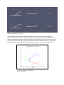
With use of the CFD computations, the pressure drop between the proximal artery and the vein, can be
determined. The pressure drop was calculated by determining the difference between the pressure at
the entrance of the proximal artery and at the end of the curvature in the vein. This results in a pressure
drop of 637 Pa (= 4.8 mmHg) for the RC-AVF and a pressure drop of 379 Pa (= 2.8 mmHg) for the BC-AVF.
The pressure drops are plotted in the graph that is obtained in ARCH Deliverable D5.3 (11) while using the
corresponded ratio vein/artery of 1 (fig. 3.7).
Figure 3.7: Relation between pressure drop and Reynolds number, adapted from D5.3
It can be seen that the pressure drop determined with the current RC-AVF and BC-AVF geometries, is
ten times lower than previously. The difference between RC-AVF and BC-AVF is the result of a difference
in flow, flow division and diameter.
20
4. Discussion & Conclusion
The aim of the project was to validate the geometrical characterization proposed in D5.3 and to obtain
patient-based function parameters for both RC-AVF and BC-AVF; and to use the geometrical
characterizations for meshing in CFD simulations. To achieve this, CE-MRA data of 12 patients was used.
Subsequently, the segmentation results were fitted with parameterized functions. The fitted parameters
were averaged to obtain a generic RC-AVF and BC-AVF mesh, which can be used for 3D CFD simulations.
In the next sections each analysis step is evaluated. Hereafter, the main conclusions will be drawn and
recommendations will be made for further research.
4.1 AVF Segmentation
The segmentation of the post-surgical CE-MRA with the LabVAS prototype resulted in a good
determination of the AVF centerline. The determination of the vessel wall coordinates provided a good
estimate at the in- and outflow tracts. However, in the bifurcation an error occurred. This error is the
result of the vessel wall determination, which cannot distinguish between the arterial or venous wall at
the position of the anastomosis. By using the median diameter, the influence of this error in further data
evaluation is negligible.
From the segmentations it could be noted that the artery is slightly curved towards the connection
between artery and vein. This curve could be the result of the surgery, where in suturing of the vein to
the artery, the artery is pulled towards the vein. In this research the influence of this curvature is
neglected, but the effect of this curvature on the flow profiles should be analyzed.
During this research CE-MRA images are used for the AVF segmentation. CE-MRA has the benefit of
higher spatial and temporal resolution when compared to conventional MRA, duplex ultrasonography
and digital subtraction angiography (1). Nevertheless, CE-MRA is not commonly acquired. Therefore, to
include a larger patient population, the segmentation method should be adjusted, so that it can be also
be applied to conventional MRA data.
4.2 AVF Fitting
With some small adjustments the earlier proposed equations could be used to fit the obtained diameter
and centerline descriptions. The largest differences between the parameters determined during this
research and the parameters chosen in ARCH Deliverable D5.3 (11), are found for the arterial and venous
diameters, and the parameters that describe the curvature of the vein. When comparing the parameters
between RC-AVF and BC-AVF it is found that the median parameters describing the curvature for RC-AVF
and BC-AVF differ, resulting in a larger angle for the BC-AVF.
4.3 Mesh creation & CFD
The obtained parameters for RC-AVF and BC-AVF are averaged and used to generate two 3D meshes.
These meshes are used for a 3D CFD simulation. When comparing the results from the current
geometries with the previous results of D5.3 it becomes clear that, an increased arterial and venous
diameter, without changing the Reynolds number, will lead to a tenfold decrease in pressure drop.
Although, when comparing this research with Van Canneyt et al. (5), the results look comparible (see fig.
4.1). With a determined pressure drop of 4.8 mmHg and flow of 497 ml/min in the RC-AVF, this result
could be implemented in figure 4.1. In the research of Van Canneyt et al. the relation between flow and
pressure drop is determined using a fixed angle, a vein/artery ratio of 1.5 and a flow distribution of
respectively 8% and 92% towards the arterial and venous outlet. Also the diameters chosen in the
21
research of Van Canneyt et al., dart = 4mm and dvein = 6 mm, are in the range of the diameters
determined in the current research.
(5)
Figure 4.1: Pressure drop results from Van Canneyt et al. ; with artery/vein
ratio of 1.5 and fixed angles; flow rate described as the arterial inlet flow; flow
distribution of 8 and 92% towards arterial and venous outlet .
Next step is to vary the AVF geometries in the ranges determined in the current research. By changing
the diameters, several vein/artery ratio can be used to evaluate the flow/pressure distributions. By
increasing the Reynolds number, the flow through the anastomosis will become more realistic. Also the
parameters determining the curvature of the anastomosis could be adjusted to investigate the influence
of the angle in the flow/pressure distribution.
4.4 Conclusion & Recommendations
From this research it can be concluded that:
- The equations described in ARCH Deliverable D5.3 can be used to characterize the centerlines
and radii of an AVF.
- Patient-specific parameters are derived, that are clearly different from the parameters used in
ARCH Deliverable D5.3.
- Based on the AVF characterizations, population averaged RC-AVF and BC-AVF geometries, can
be generated for mesh creation and CFD modeling.
- After CFD modeling a lower pressure drop is observed as in the results of ARCH Deliverable D5.3.
For future research, it is recommended to:
- Analyse more patient data by developing a segmentation method for non contrast enhanced
MRA.
- Investigate the influence of each parameter, e.g. venous and arterial diameters, used in
equation 3.1, to find the most important parameters describing the AVF geometry and the
pressure/flow relation.
- Improve the geometrical description by accounting for the curved artery, and evaluate the
influence of this curving.
- Perform more CFD simulations with different Reynolds numbers (flows), flow ratios and
geometries in order to obtain a description of the pressure-flow relation of an anastomosis to
use in a pulse wave propagation model.
22
Acknowledgments
I would like to thank the people at the Mario Negri Institute for helping me start my internship at the
beautiful Villa Camozzi. Of those people I would especially like to thank Katia Passera, who was my
coach, and Luca Antiga, for his feedback during my internship and for providing me the CFD simulations
used in this report.
I also would like to thank Frans van de Vosse for giving me the opportunity to let me finish my
internship, at the Maastricht University.
Finally I would like to thank Jeire Steinbuch, for helping me understand VMTK and Paraview for the
mesh creation and visualization.
23
24
Bibliography
1. Hemodialysis vascular access imaging. Planken, R.N. s.l. : Datawyse, Universitaire Pers Maastricht,
2006. ISBN: 978-90-5278-624-7.
2. Numerical and experimental study of blood flow through a patient-specific arteriovenous fistula used
for hemodialysis. Kharboutly, Z. and Deplano, V. s.l. : Medical Engineering & Physics, Elsevier Ltd, 2009,
Vols. 32: 111-118.
3. A primer on the av fistula - Achilles' heel, but also Cinderella of haemodialysis. Konner, K. s.l. : Nephrol
Dial Transplant, 1999, Vols. 14: 2094-2098.
4. The Arteriovenous Fistula. Konner, K. and Nonnast-Daniel, B. s.l. : J Am Soc Nephrol, 2003, Vols. 14:
1669-1680.
5. Hemodynamic impact of anastomosis size and angle in side-to-end arteriovenous fistulae: a computer
analysis. Van Canneyt, K. and Pourchez, T. s.l. : J. Vasc. Access, 2010, Vols. 11: 52-58.
6. Factors associated with early failure of arteriovenous fistulae for haemodialysis access. Wong, V. and
Ward, R. s.l. : Eur J Vasc Endovasc Surg, 1996, Vols. 12: 207-213.
7. Development of an ex vivo model to investigate the effects of altered haemodynamics on human
bypass grafts. Armstrong, J. and A.J., Narracott. s.l. : J Med Technol, 2000, Vols. 24 (5): 183-191.
8. Pulse wave progation in a model human arterial network: Assesment of a 1-D numerical simulations
against in vitro measurements. Matthys, K.S. and J., Alastruey. s.l. : J Biomech, 2007, Vols. 40:3476–
3486.
9. A lumped model for blood flow and pressure in the systemic arteries based on an approximate velocity
profile function. Huberts, W. and Bosboom, E.M.H. s.l. : Mathematical biosciences and engineering,
2009, Vols. 6 (1): 27-40.
10. A wave propagation model of blood flow in large arteries using an approximate velocity profile
function. Bessems, D., Rutten, M.C.M and van de Vosse, F.N. s.l. : J Fluid Mech, 2007, Vols. 580: 145168.
11. Database of non-linear resistance models of selected vascular tracts with complex geometry. ARCH
Deliverable D5.3. 2010.
12. Hemodynamic assesment prior to surgery by combining MRI segmentation with pulse wave
propagation simulation. Merkx, M.A.G. In progress.
13. Curve and shape exxtraction with minimal path and level-sets techniques - Applications to 3D
Medical Imaging. Deschamps, T. s.l. : PhD thesis, Unersité Paris-IX Dauphine, Place du maréchal de
Lattre de Tassigny, 75775 Paris Cedex, 2001.
25
14. Automatic contour propagation in cine cardiac magnetic resonance images. Hautvast, G, et al. s.l. :
IEEE Trans Med Imaging, 2006, Vols. 25 (11): 1472-1282.
15. Computing a trust region step. Moré, J.J. and D.C., Sorensen. s.l. : SIAM J. Sci. Stat. Comput., 1983,
Vols. 4 (3): p553-572.
16. A pressure-correction scheme for convection dominated incompressible flows with discontinuous
velocity and continuous pressure. Botti, L. and Di Pietro, D.A. s.l. : J Comp Phys submitted, 2010.
26
Appendix
In Appendix A the user manual of the LabVAS software tool, created as part of this internship, is given.
The parts in the user manual that are not used during this research or not yet described are indicated
with … .
In appendix B the patient-specific fitting results are given.
Appendix A: User Manual LabVAS
A1. Introduction LabVAS
A1.1 About LabVAS Prototype
The Laboratory prototype for Vascular Access Surgery (LabVAS) incorporates a patient-specific modeling
framework for hemodynamic assessment of End-Stage Renal Disease (ESRD) patients. This framework
combines an innovative image segmentation technique, to extract the vascular topology, with a 1D
wave propagation model approach (Kroon, 2010 [1]) and a visualization toolkit to show the simulated
hemodynamic state of the patient in an intuitive manner. To obtain patient-specific hemodynamic
predictions, a 1D model requires distributed measurements of the geometry (diameters) and topology
(connectivity) of the vascular tree, local flow measurements and blood pressure. The prototype can
obtain the geometrical and topological parameters from Contrast Enhanced MRA (CE-MRA) in the semiautomatic segmentation process. For the flow measurements the user needs QFlow MRA. The user can
obtain the flow by using the QFlow measurement function in the ViewForum environment.
The tasks that can be executed in this prototype are:
-
Registration
Segmentation
Fuse and Intervention
QFlow measurements
Simulation settings
CE-MRA images are acquired with the protocols for the ARCH project. With the protocol a proximal
(upper arm) and a distal (lower arm) CE-MRA was obtained. This is a two-stage imaging technique with
patient repositioning.
The prototype was set up in the rapid prototyping environment EasyScil 7.0 (based on ViewForum
R8.1V1L2) of Philips Medical Systems (PMS).
The general layout of the user interface (UI) of the prototype contains an area for session selection and
for stepping through the task chain, an area for the handling of the tasks and an area for viewing the
results of the task worked on. The main part of the UI is reserved for the viewing of the results of the
task to give as much visual information as possible. The interaction required from the user is reduced to
some simple steps to keep the prototype as user-friendly as possible.
27
Examples of the UI for the different steps will be shown and described in sections 1.2-1.7. A more
detailed description of the UI and the functionality is given in section 2.
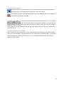
A1.2 User and input data selection.
To start the LabVAS prototype, the user has to select the image data of the patient from the image
database in the ViewForum environment and then switch to the EasyScil application. In the EasyScil
application the prototype has to be started by clicking the LabVAS icon (see chapter 2), afterwards the
user can proceed through the steps of the task chain.
The first task is to select or create a username, for which the program initiates a dedicated userdirectory on the hard disk (figure 1.1a). The second task is to select the specific data the user wants to
use for further examinations (figure1. 1b).
a.
Entering user selection
b.
Figure 1.1: User interface for user and data selection
Input data selection
A1.3 Image registration
When the user selected two or more images, and no bifurcation is present in the overlapping part of the
volumes, to automatically register the segmentations, image registration is necessary (figure 1.2). The
user has to provide at least three fiducial markers in both volumes, by scrolling through the datasets and
identifying areas of correspondence. This is the manual initialization step, required before automatic
optimalization can be performed. The latter step is executed on request of the user by clicking the
register button. The quality of registration can be inspected by using overlap images, or a binary masker.
28
Figure 2.2: User interface Image registration
A1.4 Image segmentation
The segmentation of the vessel is divided into three steps (figure 1.3):
a. Centerline creation: The creation of the centerline is initiated by a user-defined seed point in
the most proximal artery of the imaged volume. The algorithm to distinguish vessel structures
from background is the fast marching algorithm as described by Deschamps 2001 [2]. To
manage the tree-like structure during the wave front expansion process, a tree administration
algorithm was applied (Bülow et al., 2004 [3]). Tree hierarchy was introduced by defining every
component as a branch, starting at the seedpoint or bifurcation and ending at a termination
point or bifurcation. Each branch is subdivided into segments. Every segment was evaluated
during the growing process, to decide whether to continue with the next segment, continue
with a new branch or to terminate the branch. This evaluation involved calculations of the local
probability and the direction of the blood vessel (Frangi et al., 1998 [4]). The now created
centerlines were coarse, therefore the centerlines were recentered using an open active
contour model (Hautvast et al., 2006 [5])
The result of the automatic centerline detection algorithm was presented to the user for
verification. In case of disagreement the user could alternate the centerlines by cutting away or
shortening branches, and by adjustment of the centerline position.
b. Centerline sampling: In this step the user can automatically set up the diameter measurement
locations on each the centerline. The vessel contour will be extracted at these discrete points
along the centerline. Afterwards, the user can inspect the preview of the diameter
measurements and optionally delete measurements.
c. Diameter extraction: The measurement locations, initiated in the previous step, are
subsequently analyzed with an edge detection algorithm. At every measurement location,
twenty radial rays were casted perpendicular to the local vessel direction. The local vessel
contour was extracted by applying the Full-Width at Half-Maximum (FWHM) criterion.
Subsequently, the enclosed area (A) was used to determine the local diameter of the vessel by
.
29
The user can save the created centerline, the sampled centerline and the diameter extraction by using
the import/export functionality. Although the program saves all changes to a temporary file for undo
possibility, the user should store the final result manually.
a.
Starting screen image segmentation
b. Import/Export screen opened and centerlines visible
Figure 1.3: User Interface for image segmentation
A1.5 Fuse and intervention
In the fuse and intervention task the user can fuse and tag, filter his/her segmentation (figure1.4). In this
task it is also possible to construct a patient model and to perform a surgical operation. In the user
interface, this is divided in four steps.
a. Fuse and tag MR seg: In this step the segmented image can be fused. During the fusing it is
possible to merge the segmentations of the proximal and the distal MRA images. The proximal
blood vessels in the distal scan will be aligned with the distal vessels in the proximal scan using
an implementation of the Iterative Closest Point (ICP) method (Besl et al., 1992 [6]). This ICP
method searches for the optimal transformation between two clouds, in this case the points
along the vessel centerlines in the region of interest. For evaluation of the merged
segmentation, the distance between centerline points and the distance between the bifurcation
points of both segmentations were compared prior and after the registration steps. The
bifurcation point was arbitrarily defined as the point where the bifurcating centerlines of the
segmentation have distance > 0.1 mm.
In this step the user can also tag and name the different arteries or veins that are used during
segmentation and fusing process. After fusing and tagging the fusion can be stored, as a result, a
xml-file is generated in the created folder on the hard drive. With this xml-file it is possible to do
further detailed investigation of the geometry and topology on other platforms.
b. Filter and store MR seg:
…
c. Construct patient model:
…
d. Perform surgical procedure:
…
30
Figure 1.4: User interface for Fuse and intervention
1.6 QFlow measurements
Figure 1.5: User interface QFlow Measurements
…
31
A1.7 Simulation settings
Figure 1.6: User Interface Simulation settings
…
A2. Functional description
In this chapter the functionality of the user interface is described in greater detail. For general
information of every button the user can move the mouse pointer towards the button in the prototype.
ViewForum (VF) is started via the xEasyScilARCH file to which a shortcut should be located on the
desktop. The user has to log in to ViewForum with the username and password that has been generated
for him/her.
A2.1 Patient data selection
From the “Worklist” in the ViewForum environment the user has to select the data he/she wants to
analyze. To select the images needed for the prototype the user first has to select the patient folder
he/she wants to work on. In the “Series” tab at the lower part of the VF window the user can then select
the separate series that are required. To do proper analyses CE-MRA series are needed. Possible series
that the user may select are:
- DIST 3D CE CLEAR
- PROX 3D CE CLEAR
Multiple data series can be selected by using the CTRL-button or by pressing the middle mouse button.
To switch to the EasyScil facility the function “Analysis\EasyScil prototyping…” has to be used.
Having started the EasyScil facility you can use the “door handle” button to go back to the
ViewForum facility to select another dataset.
32
A2.2 Starting the prototype
The button for starting the prototype can be found on the so-called “Prototype Applications”
panel that pops up (turned blue) when pushing the “magic hat” button.
Pressing this button will start the Advanced Vessel Analysis prototype. When the prototype has
been started, a task chain will appear.
These buttons can be used to go back (<) and forward (>) in the prototype
tasks. The current location in the analysis framework is visualized with the
dot. It is possible to skip tasks by directly clicking the circle of the analysis
step of choice, or exit the prototype by pushing the “exit” button. When pushing “exit” all data, if not
saved, will be lost.
A2.3 Task 1: Entering User selection
The first task is the User selection (fig. 2.1). Here the username of the prototype have to be selected. A
new user can be included by using the text box near the “Add” button, by pressing “Add”. The selected
user is visualized with the blue bar. Here, the user “test” is selected. After selection, the “Confirm”
button has to be pressed.
33
Figure 2.1: User selection
Figure 2.2: Input Data Selection
A2.4 Task 2: Input Data Selection
The second task is to select the data you need (fig. 2.2). The CE-MRA scans acquired in the ARCH
protocol contain typically 4 time instances. By default the second instance is selected per volume, since
this is usually the scan with most arterial enhancement and absence of venous enhancement. The user
can change to a different time instance by selecting the image. By clicking on the name of the data a 3D
(MIP) picture of the data is visualized on the screen. Multiple data can be selected (blue bar) by pressing
the middle mouse button. The upper text box displays the data visualized on the screen. After selecting
one or two images, press “Confirm”.
A2.4.1 General image interaction
In the prototype the main window is used for viewing the results of the task. The user can interact with
these images in the following ways. By pressing the left mouse button and moving the mouse, the user
can interact with the image. To change the light intensity of the image, press the middle (or scroll)
button of the mouse. With the right mouse button the user can get some toolbars to change the view,
window and interaction and to get some image-information (fig. 2.3). The toolbars can be closed by
34
pressing the square at the upper-right corner. The image-interaction is indicated at the bottom left of
the image and can be changed by clicking on the icon or by using the interaction-toolbar. By holding the
middle button + right button, and dragging the mouse up or down, the zoom factor is regulated. By
holding the middle button + left button, and dragging the mouse, the image viewer is translated.
a. View toolbar
b. Window toolbar
c. Interaction toolbar
Figure 2.3 Image toolbars
d. Information toolbar
A2.5 Task 3: Image registration
When two dataset are selected, image registration is the next task. If only one dataset is selected, this
step can be skipped and the software automatically goes to the next task.
…
35
A2.6 Task 4: Image Segmentation
In this task, the user executes the image segmentation. This has to be done step-by-step, indicated with
1, 2 and 3 (fig. 2.4).
Figure 2.4: Image Segmentation
Figure 2.5: Image Segmentation; editing centerline
- Create a centerline.
To create a centerline the user has two options:
With this button a centerline with only one seeding point can be created by clicking on a blood
vessel in the image. With option “down”, turned on, the centerline will follow the artery from
head to feet direction, including all sidebranches. With option “up”, the centerline will be
formed from feet to head direction.
By pressing this button the user can create a centerline with a start and end point. The
centerline is colored green in the MIP viewer and red in the segmentation viewer. To change
between MIP and Segmentation use the bar above the image (fig. 2.5).
This button can be used to connect two branches. Depending on angle and distance, vessels are
being merged, or a bifurcation is being added.
36
With the “scissor” button the user can delete a centerline by clicking with the scissor on the
desired centerline. It is also possible to cut the centerline in two parts by CTRL+click. The
scissor-function can also be activated by pressing c.
With this button it is possible to delete small end branches. The minimum branch size of can be
indicated in the box right of this button.
All the functions can be turned off by clicking a second time on the button.
This button can used to undo the last action.
After creation of the centerline it is possible to edit the centerline by moving the pointer towards the
centerline. When the pointer is above the centerline the line highlighted. To be able to edit the
centerline, the user can click on the highlighted centerline, than the line is selected and will turn red.
Now it is possible to move the centerlinepoints in the three screens next to the main screen. When
moving the mouse up and down in the main screen while pressing the left button, the user is able to
move over the centerline by using the curved arrow interaction (fig. 2.5). The user can move points by
selecting them or delete the point by CTRL+click. A new point can be created by clicking on the
centerline. Note: after point deletion, the software does not automatically update the centerline, to
achieve this, drag and release another point of the centerline.
To store (or load) the centerline, press the” Import/Export” button to get the Import/Export screen (fig
2.6). Type a name for the centerline and press “store”. It is advisable always to store the centerline after
finalizing, because temporary files will be deleted when moving backwards in tasks (e.g. diameter
extraction to centerline extraction).
Figure 2.6: Import/Export screen
- Centerline sampling
For this the user has to choose the number of samples per cm (default 10.0) and press “generate”. Again
it is possible to change the measurement locations. Upon inspection of the measurement locations, the
user can decide to remove a location. First, the location has to be selected by clicking with left mouse
button on the measurement. Second, the measurement can be deleted by pressing the delete key on
the keyboard. When measurement locations are modified from the default, use the “Import/Export”
button to store the Centerline sampling
37
-
Diameter extraction
It is possible to do two kind of diameter extraction. When pushing the left button then
there is a single scale extraction, when pushing the right button then it is multi scale. The
single scale option performs a fast diameter extraction, based on one scale (small vessels). The
multi scale extracts diameters on a few scales and selects the optimal result. The latter method
will require more calculation time.
By pressing this button the radial distribution of the image segment can be seen while hovering
the pointer over the segmented branches. This function can also be turned on by pressing i.
With this button, the user can adapt the calculated radius manually. When moving the pointer
across the branch the user can see the change of diameter in the three separate images. By
clicking on the branch the user can freeze the image and change the diameter. The user can
move over the branch by pressing the left mouse button at the upper screen of the three
separate screens.
Again use the “Import/Export” button to store the diameter extraction. When storing the diameter
extraction, a RINGS.dat file will be generated and stored in the “segmentation\rings\(dist or prox)\art”folder. This dat-file contains information about the ring coordinates and can be used on other platforms
for further investigations.
Use the “reset” button to delete all centerlines and to start new segmentation.
A2.7 Task 5: Fuse and Intervention
In this task it is possible to fuse, filter and store the segmentation. Here it is also possible to construct a
patient model and to perform some surgical procedures. After every step the user can store the fusion,
using the “Select fusion or create new” window in the center of the screen. The fusion will be stored in
the following way:
“C:\ARCHData\(username)\(datasetname)\segmentation\networkGraphs\(fusionname)_networkGraph.xml”. The
coordinates and the radius of the centerline are stored in the .xml-file.
-
Fuse and tag MR seg
With this button the segmentation will be fused. First select the segmentations for fusion, and
then press this button. When selecting segmentations from the different dataset for fusing and
there is no bifurcation in the overlapping area, image registration is required. When registration
is required the software will automatically return to the registration task.
With this button the user can some info about the fusion and tag the different branches of the
fusion. …
-
Filter and store MR seg
With this button the user can select the filtering method. Before applying the filter the user can
38
change the filter parameters or choose the “default”. …
-
Construct patient model
…
- Perform surgical procedures
In this step it is possible to do some surgical procedures.
By pressing this button the user can create an anastomosis.
This button can be used for …
A2.8 Task 6: Qflow Measurements
…
A2.9 Task 7: Simulation settings
…
A3. Additional Information
For each image dataset loaded from the prototype’s database selector folder a folder is generated. The
folders are organized by using the username (selected in task 1), the dataset name, the kind of task and
the chosen names during Import/Export actions. The saved files in these folders can be used for further
actions of the prototype or by other software (for example the xml-files). When using the xml-file in
MatLab (The MathWorks Inc.), the user needs an extra xml-toolbox (available at www.geodise.org).
References Appendix A
1.
2.
3.
4.
5.
6.
Kroon, . 2010. On linearization, discretization and coupling of 0 and 1d models for estimating vascular hemodynamics.
Submitted.
Deschamps, T. 2001. Curve and Shape Extraction with Minimal Path and Level-Sets techniques - Applications to 3D
Medical Imaging. PhD thesis, Université Paris-IX Dauphine, Place du maréchal de Lattre de Tassigny, 75775 Paris
Cedex.
Bülow, T., Lorenz, C., and Renisch, S. 2004. A general framework for tree segmentation and reconstruction from
medical volume data. In Medical Image Computing and Computer-Assisted Intervention, Proceedings, volume 1, pages
533–540.
Frangi, A. F., Niessen, W. J., Vincken, K. L., and Viergever, M. A. 1998. Multiscale vessel enhancement filtering. In
Medical Image Computing and Computer-Assisted Intervention, Proceedings, pages 130–137. Springer-Verlag.
Hautvast, G., Lobregt, S., Breeuwer, M., and Gerritsen, F. 2006. Automatic contour propagation in cine cardiac
magnetic resonance images. IEEE Trans Med Imaging, 25(11):1472–1482.
Besl, Paul J., M. N. D. 1992. A method for registration of 3-d shapes. IEEE Transactions on Pattern Analysis and
Machine Intelligence, 14(2):239–256.
39
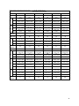
Appendix B: Patient-specific fitting results
Table B1: Patient specific fitting results of RC-AVF; (…,…) is the 95% confidence bound, e+6 means 106
Radiocephalic AVF CE-MRA Dist
PatientID
Blood vessel
x
d
a
t
a
z
d
a
t
a
a
b
rsquare
a
b
rsquare
median
diameter
Blood vessel
x
d
a
t
a
a
b
rsquare
median
diameter
Blood vessel
x
d
a
t
a
a
b
rsquare
a
y
d
a
t
a
b
c
rsquare
z
d
a
t
a
a
b
rsquare
median
diameter
20001
20003
20005
20009
20012
20015
ap
ap
ap
ap
ap
ap
9.8
(9.331, 9.585)
1.0
(1.011,1.071)
11.7
(11.71, 11.72)
1.0
(1.009,1.011)
10.1
(10.12, 10.15)
1.0
(1.014,1.023)
14.1
(14, 14.28)
1.1
(1.093,1.14)
13.2
(13.16, 13.21)
0.99
(0.9902, 0.9982)
11.3
(11.22, 11.48)
1.4
(1.353,1.418)
0.9983
1
1
0.9986
1
0.9987
4.2
(4.042, 4.436)
0.90
(0.8085,0.9986)
-1.2
(-1.255, -1.177)
0.50
(0.506, 0.6048)
-2.0
(-2.134, 1.831)
1.2
(1.047,1.439)
-5.5
(-5.814, -5.295)
0.75
(0.6655,0.8338)
1.4
(1.346, 1.367)
1.1
(1.061, 1.096)
3.1
(2.629, 3.592)
0.17
(0.01385,0.3254)
0.9792
0.9819
0.9561
0.9622
0.9993
0.4245
4.9
3.2
4.0
3.7
5.0
4.3
ad
ad
ad
ad
ad
ad
-11.0
(-11, -10.98)
1.0
(0.9976,1.002)
-5.3
(-5.359, -5.329)
0.99
(0.9865, 0.9993)
-7.1
(-7.188, -7.116)
1.1
(1.052,1.076)
-11. 6
(-11.62, -11.51)
0.99
(0.984,1.005)
-6.1
(-6.105, -6.062)
0.97
(0.9678, 0.9832)
-4.9
(-4.927, -4.89)
1.3
(1.268,1.289)
1
1
0.9998
0.9997
0.9999
0.9999
4.6
3.9
3.9
3.7
5.6
3.9
v
v
v
v
v
v
13.4
(13.18, 13.58)
0.99
(0.9554, 1.02)
10.0
(9.888, 10.06)
1.0
(1.021,1.062
11.5
(11.48, 11.62)
1.2
(1.143,1.172)
15.8
(15.68, 15.95)
1.1
(1.102,1.141)
8.7
(8.605, 8.811)
1.1
(1.083,1.139)
11.4
(11.32, 11.57)
0.83
(0.8092,0.8524)
0.9964
0.9988
0.9996
0.9988
0.9988
0.9973
0.82
(0.7177, 0.9258)
3.2
(-0.2094, 6.588)
9.1
(8.635, 9.613)
0.73
(0.2173, 1.244)
0.7
(-0.7455, 2.175)
9.9
(9.575, 10.28)
0.86
(0.8512,0.8723)
2.7
(2.513,2.973)
12.0
(11.95, 12.06)
0.86
(0.101,1.614)
0.79
(-1.234,2.809)
14.1
(13.38,14.78)
0.87
(0.7877, 0.9584)
21.32
(-111.5, 154.2)
8.7
(8.271, 9.185)
1.35e-10
(fixed at bound = 0)
1.702e-7
(no confidence bounds )
1.586
(no confidence bounds)
0.9519
0.9583
0.9997
0.9217
0.9843
0.035
6.5
(6.291, 6.687)
1.3
(1.227,1.387)
-10.5
(-10.71, 10.25)
1.4
(1.331, 1.453)
-2.9
(-3.027, -2.726)
2.3
(2.064,2.494)
-5.6
(-5.817, -5.349)
1.7
(1.541,1.805)
-1.5
(-1.628, -1.467)
1.4
(1.305, 1.606)
12.5
(12.2, 12.82)
1.3
(1.255,1.386)
0.9879
0.9943
0.9817
0.9798
0.9832
0.992
6.9
3.4
4.6
5.8
3.7
4.1
40
Table B2: Patient specific fitting results of BC-AVF; (…,…) is the 95% confidence bound
Brachiocephalic AVF CE-MRA Dist
PatientID
Blood vessel
a
xdata
b
rsquare
a
zdata
b
rsquare
median
diameter
Blood vessel
a
xdata
b
rsquare
median
diameter
Blood vessel
a
xdata
b
rsquare
a
ydata
b
c
rsquare
a
zdata
b
rsquare
median
diameter
20007
20008
20013
20018
20019
20024
ap
ap
ap
ap
ap
ap
14.0
(14, 14.1)
1.0
(0.9947, 1.011)
20.3
(20.33, 20.32)
0.99
(0.9858, 0.9961)
5.6
(5.598, 5.601)
0.99
(0.9947,0.9959)
13.1
(13.01, 13.19)
0.98
(0.9634, 0.9924)
10.5
(10.53, 10.57)
0.99
(0.9854, 0.9947)
6.6
(6.605, 6.66)
0.99
(0.9841, 1.003
0.9998
0.9999
1
0.9993
1
0.9999
-5.4
(-5.489, -5.402)
1.0
(1.008, 1.044)
9.9
(9.83, 10.08)
1.0
(1.019, 1.075)
0.74
(0.718, 0.7664)
1.2
(1.145, 1.315)
-9.8
(-9.9, -9.725)
1.1
(1.132, 1.175)
1.3
(1.181, 1.535)
3.5
(2.675, 4.27)
-1.5
(-1.669, -1.416)
1.2
(1.001, 1.423)
0.9991
0.9967
0.996
0.9989
0.9394
0.9711
3.8
4.8
5.4
4.1
6.1
6.5
ad
ad
ad
ad
ad
ad
-15.4
(-15.44, -15.41)
1.0
(1.022, 1.027)
-12.2
(-12.2, -12.17)
1.0
(1.016, 1.02)
-6.1
(-6.117, -6.113)
1.0
(1.006, 1.007)
-7.5
(-7.536, -7.47)
1.1
(1.078, 1.099)
-4.8
(-4.811, -4.744)
1.0
(0.9687, 1.001)
-2.9
(-2.937, -2.935)
1.0
(0.9956, 0.9978)
1
1
1
0.9999
0.9998
1
3.4
4.2
4.8
3.6
5.7
5.3
v
v
v
v
v
v
13.1
(12.83,13.42)
1.3
(1.267, 1.387)
15.8
(15.62, 16.02)
1.5
(1.488, 1.561)
4.9
(4.755, 4.959)
1.5
(1.449, 1.572)
10.3
(10.14,10.47)
0.88
(0.8442, 0.9092)
5.2
(5.117, 5.22)
1.3
(1.251,1.302)
6.1
(6.013, 6.294)
1.7
(1.655, 1.805)
0.9914
0.9975
0.9956
0.9942
0.9993
0.9962
0.39
(-0.5253, 1.306)
0.56
(-3.256, 4.374)
7.1
(6.609, 7.654)
0.86
(0.8475, 0.8747)
2.3
(2.113,2.536)
26.2
(26.04, 26.29)
0.82
(0.4522, 1.183)
0.73
(-0.2098, 1.673)
11.6
(11.35, 11.88)
1.1
(1.09, 1.143)
15.6
(1.276, 29.99)
28.0
(27.53, 28.43)
0.93
(0.8414, 1.024)
1.3
(0.8357, 1.677)
10.0
(9.872,10.09)
0.94
(0.8976, 0.9853)
0.89
(0.7688, 1.015)
10.9
(10.9, 10.97)
0.6679
0.9994
0.9877
0.9979
0.9985
0.9998
13.6
(12.99, 14.16
0.98
(0.8865, 1.069)
6.7
(6.347, 7.126)
2.0
(1.817, 2.242)
10.2
(9.986, 10.45)
1.5
(1.404, 1.534)
-7.9
(-8.089, -7.733)
2.0
(1.885, 2.047)
4.5
(4.412, 4.66)
1.7
(1.639, 1.821)
6.7
(6.472, 6.871)
1.2
(1.144, 1.295)
0.9658
0.9619
0.9952
0.9944
0.9961
0.9923
5.1
8.0
4.2
7.8
3.9
4.8
41