Download User Manual for PileAXL 2014

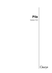
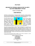
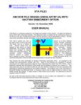
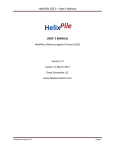
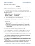
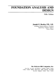
 User Manual for PileAXL 2014
A Program for Single Piles under Axial Loading
By
Innovative Geotechnics Pty Ltd
Gibraltar Circuit, Parkinson, QLD, 4115
Australia
February 2015
Important Warning:
Please carefully read the following warning and disclaimers before downloading or using the
software and its accompanied user manual.
Although this software was developed by Innovative Geotechnics Pty Ltd in Australia with
considerable care and the accuracy of this software has been checked and verified with many
tests and validations, this software shall not be used for design unless the analysis results
from this software can be verified by field testing and independent analyses and design from
other parties.
The users are responsible for checking and verifying the results and shall have a thorough
and professional understanding about the geotechnical engineering principles and relevant
design standards.
In no event shall Innovative Geotechnics Pty Ltd and any member of the organization be
responsible or liable for any consequence and damages (including, without limitation, lost
profits, business interruption, lost information, personal injury, loss of privacy, disclosure of
confidential information) rising from using this software.
Table of Contents
Chapter 1. Introduction
1
Chapter 2. Start the new file
2
Chapter 3. Project Title Information Input
4
Chapter 4. Analysis Option Input
6
Chapter 5. Pile Type and Cross Section Input
9
Chapter 6. Pile Length Input
14
Chapter 7. Soil Layers and Properties Input
16
Chapter 8. Pile Load Input
24
Chapter 9. Review Input Text File
26
Chapter 10. Reviewing Soil Layer Input Parameters
27
Chapter 11. Reviewing Pile Input Parameters
29
Chapter 12. Run Analysis
31
Chapter 13. Viewing Analysis Results
33
Chapter 14. Viewing T-Z Curves
39
Chapter 15. Viewing Q-W Curves
43
Chapter 16. Pile Axial Load Settlement Curve
47
Chapter 17. Axial Load Transfer Curve
51
Appendices
Appendix A. T-Z curves for axial force analysis
54
Appendix B. Examples
87
References
98
List of Figures
Figure 2-1 Project start dialog in PileAXL 2014
Figure 2-2 Default analysis file of PileAXL 2014
Figure 2-3 Analysis file selection dialog for PileAXL 2014
Figure 3-1 Invoke “Project Title” dialog from the menu
Figure 3-2 Invoke “Project Title” dialog from the toolbar
Figure 3-3 General layout of “Project Title” Dialog
Figure 4-1 Invoke “Analysis Option” dialog from the menu
Figure 4-2 Invoke “Analysis Option” dialog from the toolbar
Figure 4-3 General Layout of Analysis Option Dialog for PileAXL 2014
Figure 4-4 Plug settings for steel open-ended driven piles
Figure 5-1 Invoke “Pile Section” dialog from the menu
Figure 5-2 Invoke “Pile Section” dialog from the toolbar
Figure 5-3 General Layout of Pile Type and Cross Section Dialog
Figure 5-4 Section Input Dialog for Pipe Section
Figure 5-5 Section Input Dialog for Circular Cross Section
Figure 5-6 Section Input Dialog for Circular Cross Section
Figure 5-7 Section Input Dialog for Octagonal Cross Section
Figure 5-8 Section Input Dialog for H Section
Figure 6-1 Invoke “Pile Length” dialog from the menu
Figure 6-2 Invoke “Pile Length” dialog from the toolbar
Figure 6-3 General Layout of Pile Length Input Dialog
Figure 7-1 Invoke “Soil Layers and Properties” dialog from the menu
Figure 7-2 Invoke “Soil Layers and Properties” dialog from the toolbar
Figure 7-3 Soil Layers and Properties Input for the first layer
Figure 7-4 Soil Layers and Properties Input for the cohesive soils – Basic Parameters
Figure 7-5 Soil Layers and Properties Input for the cohesive soils – Advanced Parameters
Figure 7-6 Soil Layers and Properties Input for the cohesionless soils – Basic Parameters
Figure 7-7 Soil Layers and Properties Input for the cohesionless soils – Advanced Parameters
Figure 7-8 Soil Layers and Properties Input for the rock – Basic Parameters
Figure 7-9 Soil Layers and Properties Input for the rock – Advanced Parameters
Figure 7-10 Typical Ground Profile after Soil Layer Input
Figure 7-11 Copy ground profile graph from the “File” Menu
Figure 7-12 Copy ground profile graph from the “File” Menu
Figure 8-1 Invoke “Pile Top Loading” input dialog from the menu
Figure 8-2 Invoke “Pile Top Loading” input dialog from the toolbar
Figure 8-3 Pile Top Loading Input Dialog
Figure 9-1 Open Input Text File for review from the toolbar
Figure 9-2 Generated Input Text File for this example
Figure 10-1 Open soil layer input summary table for review from the menu
Figure 10-2 Open soil layer input summary table for review from the left toolbar
Figure 10-3 Soil layer input summary table for an example
Figure 11-1 Open pile input summary table for review from the menu
Figure 11-2 Open pile input summary table for review from the left toolbar
Figure 11-3 Pile input summary table for an example
Figure 12-1 Open “Run Analysis” dialog from the menu
Figure 12-2 Open “Run Analysis” dialog from the top toolbar
Figure 12-3 Run Analysis Message Box for an example
Figure 13-1 Open the “Analysis Results” Output Dialog from the left toolbar
Figure 13-2 Analysis Results Dialog for Example-1
Figure 13-3 Viewing the analysis results from the menu items
Figure 13-4 Open “Tabulated Analysis Results” dialog from the menu
Figure 13-5 Open “Tabulated Analysis Results” dialog from push button
Figure 13-6 Tabulated Analysis Results Dialog for Example-1
Figure 13-7 Copied result graph (combined Plot – Ultimate) for an example
Figure 14-1 Open “T-Z Curve Plot” dialog from the menu
Figure 14-2 Open “T-Z Curve Plot” dialog from the toolbar
Figure 14-3 “T-Z Curve Plot” dialog for an example
Figure 14-4 Tabulated T-Z Curve results for an example
Figure 14-5 Copied T-Z curves graph for an example
Figure 15-1 Open “Q-W Curve Plot” dialog from the menu
Figure 15-2 Open “Q-W Curve Plot” dialog from the left toolbar
Figure 15-3 “Q-W Curve Plot” dialog for an example
Figure 15-4 Tabulated H-Y Curve results for Example-1
Figure 15-5 Copied Q-W Curve Plot for an example
Figure 16-1 Open “Axial Load Pile Settlement” dialog from the menu
Figure 16-2 Open “Axial Load Pile Settlement” dialog from the left toolbar
Figure 16-3 “Axial Load Settlement Curve” dialog for an example
Figure 16-4 Tabulated axial load settlement curve results for Example-1
Figure 16-5 Copied axial load pile settlement curve for Example-1
Figure 17-1 Open “Axial Load Distribution vs Depth” dialog from the menu
Figure 17-2 Open “Axial Load Distribution vs Depth” dialog from the left toolbar
Figure 17-3 “Axial Load Transfer Curve” dialog for an example
Figure A.1-1 t-z curve adopted for the cohesive and cohesionless soils – driven piles (after
API 2000)
Figure A.1-2 q-w curve adopted for the cohesive and cohesionless soils – driven piles (after
API 2000)
Figure A.1-3 Basic soil parameter input of API method for cohesive soils
Figure A.1-4 Advanced soil parameter input of API method for cohesive soils
Figure A.1-1 P-Y curve for soft clay (Matlock) model under static loading condition
Figure A.1-5 Variation of the adhesion factor with the undrained shear strength (after USACE,
1991)
Figure A.1-6 Basic soil parameter input of USACE method for cohesive soils
Figure A.1-7 Advanced soil parameter input of USACE method for cohesive soils
Figure A.1-8 General procedure of calculating the ultimate shaft resistance for cohesive soils
based on ICP method
Figure A.1-9 General procedure of calculating the ultimate end bearing resistance for
cohesive soils based on ICP method
Figure A.1-10 Basic soil parameter input of ICP method for cohesive soils
Figure A.1-11 Advanced soil parameter input of ICP method for cohesive soils
Figure A.1-12 Advanced soil parameter input of User Defined method for cohesive soils –
Driven Piles
Figure A.1-13 t-z curve adopted for the cohesive soils – bored piles (FHWA,1999)
Figure A.1-14 q-w curve adopted for the cohesive soils – bored piles (FHWA,1999)
Figure A.1-15 Advanced soil parameter input of FHWA method for cohesive soils – Bored
Piles or Drilled Shafts
Figure A.1-16 Advanced soil parameter input of User Defined method for cohesive soils –
Bored Piles or Drilled Shafts
Figure A.2-1 Basic soil parameter input of API method for cohesionless soils – Driven Piles
Figure A.2-2 Advanced soil parameter input of API method for cohesionless soils – Driven
Piles
Figure A.2-3 Bearing capacity factor for cohesionless soils – Driven Piles (after USACE 1991)
Figure A.2-4 Advanced soil parameter input of USACE method for cohesionless soils – Driven
Piles
Figure A.2-5 General procedure of calculating the ultimate shaft resistance for cohesionless
soils based on ICP method (after Jardine et al. 2005)
Figure A.2-6 General procedure of calculating the ultimate end bearing resistance for
cohesionless soils based on ICP method (after Jardine et al. 2005)
Figure A.2-7 Advanced soil parameter input of USACE method for cohesionless soils – Driven
Piles
Figure A.2-8 Advanced soil parameter input of User Defined method for cohesionless soils –
Driven Piles
Figure A.2-9 Basic soil parameter input of FHWA method for cohesionless soils – Bored Piles
or Drilled Shafts
Figure A.2-10 Advanced soil parameter input of FHWA method for cohesionless soils – Bored
Piles or Drilled Shafts
Figure A.2-11 t-z curve adopted for the granular soils – bored piles (FHWA, 1999)
Figure A.2-12 q-w curve adopted for the granular soils – bored piles (FHWA, 1999)
Figure A.3-1 Basic soil parameter input of General Rock Method – Bored Piles or Drilled
Shafts
Figure A.3-2 Advanced soil parameter input of General Rock Method – Bored Piles or Drilled
Shafts
Figure B.1-1 Ground profile with the pile length and loading conditions for Example 1
Figure B.1-2 Combined plot of the pile capacity results for Example 1
Figure B.1-3 Pile axial load and settlement relationship for Example 1
Figure B.2-1 Ground profile with the pile length and loading conditions for Example 2
Figure B.2-2 Combined plot of the pile capacity results for Example 2
Figure B.2-3 Pile axial load and settlement relationship for Example 2
Figure B.3-1 Ground profile with the pile length and loading conditions for Example 3
Figure B.3-2 Combined plot of the pile capacity results for Example 3
Figure B.3-3 Pile axial load and settlement relationship for Example 3
Figure B.3-4 Comparisons between testing results and the predictions by PileAXL 2014 for
Example 3
List of Tables
Table A.1-1 T-z curve for USACE method based on the recommendation by Coyle and Reese
(1966)
Table A.2-1 Design parameters for cohesionless soils (after API 2000)
Table A.2-2 Recommended critical depth for cohesionless soils (after USACE 1991)
Table A.2-3 Recommended interface friction angle for cohesionless soils (after USACE 1991)
Table A.2-4 Recommended coefficient of lateral pressure for cohesionless soils (after USACE
1991)
Chapter 1. Introduction
PileAXL 2014 is a program that analyzes the behaviour of single piles under axial loading
applied at the pile head (compression or tension) for both onshore and offshore engineering
problems. Both bored piles and driven piles can be analysed by the program. The program
computes the ultimate and factored pile capacities for a range of pile lengths together with the
short-term pile settlement curve for a specific pile length.
User Manual of PileAXL 2014 will be presented with an example which follows the natural
flow of program use from opening a new file to result outputs. The input file (Example-1.flp)
for this example can be found within the “Examples” folder in the program installation
directory. The details about this example are presented in Appendix C.
1 Chapter 2. Start the new file
When PileAXL 2014 program is started, the following dialog (Figure 2-1) will firstly appear,
which enables the user to choose (1) Start a new project or (2) Open an existing project.
Figure 2-1 Project start dialog in PileAXL 2014
In this example, we select the first option which is “Start a new project”. Once this option is
selected, a default new project with two soil layers is automatically created. The default file
name is Newfile.AXL. The corresponding file path is shown on the top title bar of the program.
The ground profile and general program interface is loaded and shown in Figure 2-2.
If “Open an existing project” button is clicked, then the file selection dialog will be invoked as
shown in Figure 2-3 where the user will be able to open the existing PileAXL analysis file with
the file type of AXL.
2 Figure 2-2 Default analysis file of PileAXL 2014
Creating the new project which the user wants will be started from this point onwards from
modifying the existing default project settings.
Figure 2-3 Analysis file selection dialog for PileAXL 2014
3 Chapter 3. Project Title Information Input
The project title information can be updated or modified by clicking the “Title” icon from the
toolbar (Figure 3-2) or clicking “Project Title” menu item from the main “Define” menu (Figure
3-1) of the program as shown in the figures below.
Figure 3-1 Invoke “Project Title” dialog from the menu
Figure 3-2 Invoke “Project Title” dialog from the toolbar
Figure 3-3 shows the general layout of “Project Title” dialog. The following information can be
input by the user for the project:

Project Title – Example-1

Job Number - 00001

Design Engineer - IGEngSoft

Client - IGEngSoft

Description – This is Example-1 of PileAXL 2014 software
4 Figure 3-3 General layout of “Project Title” Dialog
The following items are created by the program for the user’s reference and cannot be
changed by the user from this dialog:

Date – the creation date of the project file. The date will also be updated when the project
file is changed and saved.

File name – the full file name with the directory path

File path – the directory path of the program
5 Chapter 4. Analysis Option Input
The analysis option can be updated or modified by clicking the “Analysis Option” icon from the
toolbar (Figure 4-2) or clicking “Analysis Option” menu item from the main “Define” menu
(Figure 4-1) of the program as shown in the figures below.
Figure 4-1 Invoke “Analysis Option” dialog from the menu
Figure 4-2 Invoke “Analysis Option” dialog from the toolbar
Figure 4-3 shows the general layout of “Analysis Option” dialog. This dialog provides the user
with different analysis options as described below for two main groups: (1) “Control
Parameters” Group and (2) "Units of Input and Analyses" group.
6 Figure 4-3 General Layout of Analysis Option Dialog for PileAXL 2014
"Control Parameters" group lists the main control parameters for the analysis:

Number of pile elements: This is the number of pile elements used in the analysis. The
pile length will be equally divided into elements with the specified number.
"Compression" group lists the main control parameters for the resistance factors adopted in
the analysis for pile compression capacity:

Resistance factor for shaft resistance: This is the resistance factor of the ultimate shaft
resistance. It is usually less than 1.0 and similar to strength reduction factor or partial
factor. It is mainly used to calculate the factor pile capacity in limit state design;

Resistance factor for end bearing resistance. This is the resistance factor of the ultimate
end bearing resistance. It is usually less than 1.0 and similar to strength reduction factor
or partial factor. It is mainly used to calculate the factor pile capacity in limit state design;
"Tension" group lists the main control parameters for the resistance factors adopted in the
analysis for pile tension capacity:

Resistance factor for shaft resistance: This is the resistance factor of the ultimate shaft
resistance. It is usually less than 1.0 and similar to strength reduction factor or partial
factor. It is mainly used to calculate the factor pile capacity in limit state design;
"Plug Settings" group lists the main control parameters for the plug settings of driven pile
analysis:
7 
Plugged condition for steel open-ended piles: This is for the condition where a plugged
toe is formed under the pile bottom when the steel open-ended piles are driven into the
target toe depth. The ultimate bearing capacity is calculated based on the gross section
area and only ultimate shaft resistances along the external pile shaft area are considered;

Unplugged condition for steel open-ended piles: This is for the condition where an
unplugged toe is formed under the pile bottom when the steel open-ended pies are driven
into the target depth. The ultimate end bearing capacity is calculated based on the
section area and ultimate shaft resistance both along internal and external pile shaft
areas are considered. If this option is selected, then an additional reduction factor can be
applied to the internal shaft resistance in order to consider the potential disturbing effects
on the internal friction during driving.
Figure 4-4 Plug settings for steel open-ended driven piles
"End Bearing in Layered Soils" group lists the control parameters for the ultimate end bearing
calculation within the layered soils based on the approaches recommended in Meyerhof
(1976), Meyerhof and Sastry (1978) and Matsui (1993). Two different empirical depth
parameters for upper and lower layers can be input by the user: (1) empirical depth parameter
for the upper layer X1 and (2) empirical depth parameter for the lower layer X2. Those two
parameters control the effects of upper and lower soil layers on the middle layer when the
ultimate end bearing capacity is calculated. The graph in Figure 4-3 shows the general
distribution of the ultimate end bearing resistance within the layered ground profile. Those
parameters generally range from 3 to 6 pile diameters. In PileAXL 2014, the default value is 3
pile diameters. Note that the value of 0 means that no layering effects are considered for pile
capacity and settlement analysis.
"Units of Input and Analyses" group provides two unit options in the program.

SI Units: This is to select SI Units in the program. It the default option in the program.

English Units: This is to select English Units in the program. This option is currently not
available.
8 Chapter 5. Pile Type and Cross Section Input
The pile type and cross section input can be accessed by clicking “Pile Section” item under
“Define” main menu (Figure 5-1) or clicking “Pile Section” icon on the toolbar (Figure 5-2).
Figure 5-1 Invoke “Pile Section” dialog from the menu
Figure 5-2 Invoke “Pile Section” dialog from the toolbar
Figure 5-3 shows the general layout of “Pile Type and Cross Section” dialog. We select
“Driven Pile” option for Pile Type and select “Pipe Section” for Cross Section Type.
9 Figure 5-3 General Layout of Pile Type and Cross Section Dialog
The next is to click “Edit Section Dimension” button to open the ‘Section Input” dialog as
shown below for pipe section option. For this example, we type 0.6 m for the outside diameter,
D1 and 0.56 m for the inside diameter D2. Note that if the user types a D2 value greater than
D1, then the program will automatically correct this when this dialog is closed. This is to
ensure that the reasonable section sizes are provided.
10 Figure 5-4 Section Input Dialog for Pipe Section
The next is to close this “Section Input” dialog. Note that the section properties in “Pile Type
and Cross Section” dialog will be automatically updated according to the input cross section
dimension. For Young’s modulus E, we type 200 GPa for steel material.
If required, other cross sections can be selected by the user by switching the radio button
within the group of cross section types.
Figure 5-5 Section Input Dialog for Circular Cross Section
11 Figure 5-6 Section Input Dialog for Circular Cross Section
Figure 5-7 Section Input Dialog for Octagonal Cross Section
12 Figure 5-8 Section Input Dialog for H Section
13 Chapter 6. Pile Length Input
The pile length input can be accessed by clicking “Pile Length” item under “Define” main
menu (Figure 6-1) or clicking “Pile Length” icon on the toolbar (Figure 6-2). The invoked
dialog allows the user to input the pile length and Pile Top Level.
Figure 6-1 Invoke “Pile Length” dialog from the menu
Figure 6-2 Invoke “Pile Length” dialog from the toolbar
PileAXL 2014 provides a unique interactive input (as shown in Figure 6-3) of Pile Length.
Cantilever portion of the pile as shown in the figure is denoted as "Free Length Zone (Null)".
This can be achieved by specifying a "Null" material layer at the ground surface with the layer
thickness equal to the cantilever length or free length.
14 Figure 6-3 General Layout of Pile Length Input Dialog
15 Chapter 7. Soil Layers and Properties Input
PileAXL 2014 offers an innovative and straightforward interactive way to create multiple soil
layers with various relevant parameters in the program. Soil layer input dialog can be invoked
through clicking "Soil Layers and Properties" item under "Define" menu (Figure 7-1) or
clicking "Soil Layers and Properties" icon from the toolbar (Figure 7-2).
Figure 7-1 Invoke “Soil Layers and Properties” dialog from the menu
Figure 7-2 Invoke “Soil Layers and Properties” dialog from the toolbar
In PileAXL 2014, Soil layers can be added, inserted or deleted through "Add", "Insert" and
"Delete" buttons. The layer color also can be adjusted or updated by clicking "Color" button.
16 In the current version, maximum 50 soil layers can be defined by the user. Layer name also
can be defined by the user through text input.
The available material types from “Soil Layers and Properties” input dialog include: (1) Null
material; (2) Cohesive soils; (3) Cohesionless soils and (4) Rocks. For each material type,
different analysis methods for ultimate shaft resistance and ultimate end bearing resistance
can be selected through "Advanced" tab except for Null materials which are mainly used to
model the pile cantilever (free length) section above or below water. In another word, free
length or cantilever pile length is defined through adopting a soil layer with Null material
properties at the ground surface. Once "Null Material" type is selected, the "Advanced" tab
will be disabled.
Figure 7-3 Soil Layers and Properties Input for the first layer
Input of soil layers and properties mainly consists of two parts:
(1) Basic soil parameters on "Basic" Tab such as soil layer thickness, total unit weight,
groundwater status (above or below ground water table), undrained shear strength for
cohesive soils, effective friction angle for cohesionless soils and unconfined compressive
strength for rocks. For cohesive soils and rocks, the strength increment with the layer depth
also can be specified through "Strength Parameters - Advanced" option. The strength
increment is automatically set to zero if the default option is selected.
(2) Advanced soil parameters related to different pile capacity analysis approaches on
"Advanced" Tab.
17 The available pile capacity analysis models depend on the soil type which the user select and
are listed below for different soil types and pile installation types:
Driven Piles:

Cohesive Soils: API Method, USACE Method, ICP Method and User Defined Method.

Cohesionless Soils: API Method, USACE Method, ICP Method and User Defined Method.
Bored Piles:

Cohesive Soils: FHWA Method, User Defined Method.

Cohesionless Soils: FHWA Method, Rollins’s Gravelly Sand Method, Rollins’s Gravel
Method and User Defined Method.

Rock: General Rock Method and User Defined Method
Detailed descriptions about the different pile capacity analysis methods adopted by PileAXL
2014 are presented in Appendix A.
Figure 7-3 shows the soil layer and property input for the layer with “Null” material type. Since
it is a layer with “Null” material type, the “Advanced” tab is disabled with grey colour and
cannot be clicked. If the check box of “Input Layer below Water Table” is ticked, this means
that the layer with “Null” material type is under the water table – cantilever or free length
within the water. If the check box is unticked, the input soil layer thickness represents the
cantilever or free length within the air.
Figure 7-4 Soil Layers and Properties Input for the cohesive soils – Basic Parameters
18 Figure 7-4 shows the soil layers and properties input of the cohesive soils for the basic
parameters. Three different strength options are available in PileAXL 2014: (1) undrained
shear strength for cohesive soils, effective friction angle for cohesionless soils and unconfined
compressive strength for rock; (2) SPT-N for all material types and (3) Cone Tip Resistance
for all material types. The first option is the basic option and the values input into the second
and third options will be converted into the basic option parameters during the analysis. An
advanced parameter for the strength increase with the depth is provided for cohesive soil and
rock material types. As for the cohesionless soils, if the cone tip resistance option is adopted,
then the strength increase parameter with the depth is also available to the cone tip
resistance.
Figure 7-5 shows a typical advanced parameter input dialog for the cohesive soils. Different
analysis methods can be selected from this dialog to calculate the ultimate shaft and end
bearing resistances. The available t-z and q-w curve options are also presented on the dialog.
In the current version, the best suitable t-z and q-w curve options are automatically selected
by the program according to the soil type and pile installation type.
Figure 7-5 Soil Layers and Properties Input for the cohesive soils – Advanced Parameters
Figure 7-6 shows the soil layers and properties input of the cohesionless soils for the basic
parameters. Figure 7-7 shows a typical advanced parameter input dialog for the cohesionless
soils.
19 Figure 7-6 Soil Layers and Properties Input for the cohesionless soils – Basic Parameters
Figure 7-7 Soil Layers and Properties Input for the cohesionless soils – Advanced
Parameters
20 Figure 7-8 shows the soil layers and properties input of the rock for the basic parameters.
Figure 7-9 shows a typical advanced parameter input dialog for the rock.
Figure 7-8 Soil Layers and Properties Input for the rock – Basic Parameters
Figure 7-9 Soil Layers and Properties Input for the rock – Advanced Parameters
21 Clicking different layer within the layer list will display the corresponding basic parameter. The
program will save the input parameters into the internal memory when the “Close” button at
the bottom or “X” button at the top right corner. The ground profile as shown in Figure 7-10
will be created.
Figure 7-10 Typical Ground Profile after Soil Layer Input
Figure 7-11 Copy ground profile graph from the “File” Menu
22 If “Copy Graph” item under the “File” menu is clicked as shown in Figure 7-11, then the input
ground profile can be copied into the clipboard and then pasted into the report if required. The
copied ground profile graph is shown in Figure 7-12.
Figure 7-12 Copy ground profile graph from the “File” Menu
23 Chapter 8. Pile Load Input
This chapter is to define the loading at the pile head. The dialog for the pile head loading input
can be invoked by clicking "Pile Top Loading" option under "Define" menu (Figure 8-1) or
"Pile Top Loading" icon from the toolbar (Figure 8-2). Axial force in compression or tension
can be input from the user.
Figure 8-1 Invoke “Pile Top Loading” input dialog from the menu
Figure 8-2 Invoke “Pile Top Loading” input dialog from the toolbar
Figure 8-3 shows the “Pile Top Loading” input dialog. For this example, we type 2500 kN for
axial force in compression.
24 Figure 8-3 Pile Top Loading Input Dialog
25 Chapter 9. Review Input Text File
The works carried out from Step 1 to Step 8 will create an input Text file (Example-1.TXT) for
the current example. The purpose of creating this input file is to enable the user to have a
general overview about the input parameters. This input text file can be opened by clicking
“Input File” icon from the left toolbar as shown in Figure 9-1 as below. The generated input
text file is shown in Figure 9-2.
Figure 9-1 Open Input Text File for review from the toolbar
Figure 9-2 Generated Input Text File for this example
26 Chapter 10. Reviewing Soil Layer Input Parameters
In addition to reviewing the general input text file, PileAXL 2014 also provides the user with
the option of reviewing soil layer input parameters. Soil layer input summary dialog can be
invoked through clicking "Soil Layer Input Summary" option under "Define" menu (Figure 10-1)
or "Soil Layer Input Summary" icon from the left toolbar (Figure 10-2).
Figure 10-1 Open soil layer input summary table for review from the menu
Figure 10-2 Open soil layer input summary table for review from the left toolbar
The invoked summary table is shown in Figure 10-3 which enables the user to review the
detailed soil layer parameter inputs into the analysis and spot the input errors if any.
27 Figure 10-3 Soil layer input summary table for an example
28 Chapter 11. Reviewing Pile Input Parameters
Similar to soil layer input parameters, pile input summary table can be opened through
clicking "Pile Input Summary" option under "Define" menu (Figure 11-1) or pressing "Pile
Input Summary" from the left toolbar (Figure 11-2). It summaries the values of pile input
parameters from the user. Multiple columns for different pile segments can be shown if more
than one pile segment is used. The dialog as shown in Figure 11-3 enables the user to review
the input parameters related to the pile type, section type, section dimension, material
stiffness, top connection conditions, bending stiffness and pile batter.
Figure 11-1 Open pile input summary table for review from the menu
Figure 11-2 Open pile input summary table for review from the left toolbar
29 Figure 11-3 Pile input summary table for an example
30 Chapter 12. Run Analysis
Running the analysis file with the input parameters created from the previous steps can be
invoked by clicking "Run Analysis" option under "Analyze" menu (Figure 12-1) or clicking
“Run Analysis” icon from the top toolbar (Figure 12-2).
Figure 12-1 Open “Run Analysis” dialog from the menu
Figure 12-2 Open “Run Analysis” dialog from the top toolbar
The invoked running message dialog as shown in Figure 12-3 details the analysis information
and the analysis result status. The warning messages if any will be displayed under the
progress bar to show the likely cause of the problem. Clicking "OK" button will close the
dialog and the user will be able to access the various analysis results if the analysis run is
successful. Otherwise, the user will need to review the input file to find out why the analysis
cannot be successfully completed.
31 Figure 12-3 Run Analysis Message Box for an example
32 Chapter 13. Viewing Analysis Results
PileAXL 2014 provides an easy way to access various analysis results through "Analysis
Results" Output Dialog. The User can view almost all analysis results plotted against the
depth or elevation.
Clicking the corresponding radio button enables the User to switch different analysis result
plots conveniently. Soil layers with the specified layer colours and boundaries are also shown
in the graph to help the user to know the relative position of the results to the soil layers.
This “Analysis Results” Output Dialog can be invoked by clicking “Analysis Results” icon from
the left toolbar as shown in Figure 13-1.
Figure 13-1 Open the “Analysis Results” Output Dialog from the left toolbar
The “Analysis Results” Output dialog is shown in Figure 13-2. The analysis results which are
available for viewing from this dialog include:

Distribution of the ultimate unit shaft resistance with the pile length;

Distribution of the ultimate total shaft resistance with the pile length;

Distribution of the ultimate end bearing resistance with the pile length;

Distribution of the ultimate total pile capacity (ultimate total shaft resistance plus ultimate
end bearing resistance) with the pile length;

Combined plot of the ultimate total shaft resistance, ultimate end bearing and ultimate
total pile capacity against the pile length;

Distribution of the factored total shaft resistance with the pile length;

Distribution of the factored end bearing resistance with the pile length;

Distribution of the factored total pile capacity (ultimate total shaft resistance plus ultimate
end bearing resistance) with the pile length;
33 
Combined plot of the factored total shaft resistance, ultimate end bearing and ultimate
total pile capacity against the pile length;

Distribution of the effective vertical stress with the pile length;

Distribution of the pile weight with the pile length;

Distribution of the ultimate tension capacity; and

Distribution of the factored tension capacity.
Figure 13-2 Analysis Results Dialog for Example-1
The above results can also be viewed by clicking the corresponding items under the “Display”
menu as shown in Figure 13-3.
34 Figure 13-3 Viewing the analysis results from the menu items
In addition to the plotting results, PileAXL 2014 also provides the detailed analysis results in
the excel-like table format. It is convenient for the user to go through each analysis result at
different depths. The tabulated results can be also easily copied into the third-party software
for further process if required. The tabulated results can be accessed through clicking
“Tabulated Analysis Results” item under the “Display” menu (Figure 13-4) or clicking “Results
Table” button from the analysis result dialog (Figure 13-5).
35 Figure 13-4 Open “Tabulated Analysis Results” dialog from the menu
Figure 13-5 Open “Tabulated Analysis Results” dialog from push button
The tabulated analysis results are shown in the figure below. Note that the colour of each row
follows the colour of the soil layer for which the analysis results are shown. As mentioned
before, this software feature allows the user to quickly spot the results for different soil layers.
36 Figure 13-6 Tabulated Analysis Results Dialog for Example-1
PileAXL 2014 also enables the user to copy or print the relevant results on the graph. This
can be done by clicking “Copy Graph” or “Print Graph” on the bottom of the “Analysis Results”
Dialog. The copied graph can be easily pasted into the third-party application for reporting
purpose. A sample of the copied and pasted result graph is shown in Figure 13-7 for an
example.
37 Figure 13-7 Copied result graph (combined Plot – Ultimate) for an example
38 Chapter 14. Viewing T-Z Curves
In PileAXL 2014, once the analysis is successfully completed, the user can access the
various analysis results. The dialog for t-z curve plot can be invoked by clicking the "P-Y
Curve Plot" option under "Display" menu (Figure 14-1) or “P-Y Curve Plot” from the toolbar
(Figure 14-2).
Figure 14-1 Open “T-Z Curve Plot” dialog from the menu
Figure 14-2 Open “T-Z Curve Plot” dialog from the toolbar
39 T-Z curves for all the nodes can be selected and viewed by the user through T-Z Curve Plot
Dialog as shown in Figure 14-3. Plot or update the T-Z curve plots can be done through the
following steps:

Step 1: Tick the check box for the pile node number where you want to view the results.
Note that multiple node points can be selected;

Step 2: Click the "Plot/Update" button at the bottom of the table to update the T-Z curve
plots.
For each node point listed in the table, other relevant information such as Depth, Level,
Ultimate Unit Shaft Resistance, and T-Z model type are also displayed for the user's
information. The background colour of row in the table follows the colour of the soil layer.
Figure 14-3 “T-Z Curve Plot” dialog for an example
40 If required, detailed T-Z curve results can be accessed through clicking the button of "Results
Table" under the summary table. A new window with gird-type outlook as shown in Figure 144 will be invoked with "z" settlement (mm) and "fs" mobilised shaft resistance (kPa) for the
selected node points.
Figure 14-4 Tabulated T-Z Curve results for an example
PileAXL 2014 also enables the user to copy or print the relevant results on the graph. This
can be done by clicking “Copy Graph” or “Print Graph” on the bottom of the “Analysis Results”
Dialog. The copied graph can be easily pasted into the third-party application for reporting
purpose. A sample of the copied and pasted result graph is shown in Figure 14-5 for this
example.
41 Figure 14-5 Copied T-Z curves graph for an example
42 Chapter 15. Viewing Q-W Curves
In addition to T-Z curves, the user also can access Q-W curve information once the analysis
is successfully completed in PileAXL 2014. The dialog for Q-W curve plot can be invoked by
clicking the "Q-W Curve Plot" option under "Display" menu (Figure 15-1) or “Q-W Curve Plot”
from the toolbar (Figure 15-2).
Figure 15-1 Open “Q-W Curve Plot” dialog from the menu
Figure 15-2 Open “Q-W Curve Plot” dialog from the left toolbar
The invoked “Load Deflection Curve for Pile Base” dialog is shown in Figure 15-3.
43 Figure 15-3 “Q-W Curve Plot” dialog for an example
The option of “Q-W Curve Plot” shows the relationship between the end bearing resistance
and pile toe settlement. If required, the tabulated results as shown in Figure 15-4 for the load
and deflection curves at the pile base will be presented in the Excel-like table format through
clicking the button of "Results Table" under the graph.
44 Figure 15-4 Tabulated H-Y Curve results for Example-1
PileAXL 2014 also enables the user to copy or print the relevant results on the graph. This
can be done by clicking “Copy Graph” or “Print Graph” on the bottom of “Load Deflection
Curve for Pile Head” dialog. The copied graph can be easily pasted into the third-party
application for reporting purpose. A sample of the copied and pasted result graph is shown in
Figure 15-5 for this example.
45 Figure 15-5 Copied Q-W Curve Plot for an example
46 Chapter 16. Pile Axial Load Settlement Curve
The dialog for pile settlement curve plot can be invoked by clicking the "Axial Load Settlement
Curve" option under "Display" menu (Figure 16-1) or “Axial Load Settlement Curve” icon from
the toolbar (Figure 16-2).
Figure 16-1 Open “Axial Load Pile Settlement” dialog from the menu
47 Figure 16-2 Open “Axial Load Pile Settlement” dialog from the left toolbar
Figure 16-3 “Axial Load Settlement Curve” dialog for an example
Figure 16-3 shows the “Axial Load Settlement Curve” dialog for an example. Load-settlement
curve is generated by the program for the specified axial loading at the pile head. Preliminary
estimations on the ultimate shaft resistance, ultimate end bearing resistance and ultimate
axial pile capacity are carried out by the program and the preliminary results are shown on the
48 load-settlement curve graph. Since the load settlement curve covers a much wider settlement
range in order to present a more complete picture, the pile head settlement corresponding to
the input axial load is shown on the graph with the arrow pointing to the right axis. The arrow
pointing to the bottom axis shows the input axial load at the pile head.
If required, the tabulated results as shown in Figure 16-4 for the load and settlement curve at
the pile head will be presented in the Excel-like table format through clicking the button of
"Results Table" under the graph.
Figure 16-4 Tabulated axial load settlement curve results for Example-1
49 PileAXL 2014 also enables the user to copy or print the axial load settlement curve results on
the graph. This can be done by clicking “Copy Graph” or “Print Graph” on the bottom of “Load
Deflection Curve for Pile Head” dialog. The copied graph can be easily pasted into the thirdparty application for reporting purpose. A sample of the copied and pasted result graph is
shown in Figure 16-5 for this example.
Figure 16-5 Copied axial load pile settlement curve for Example-1
50 Chapter 17. Axial Load Transfer Curve
In addition to the axial load and settlement curve at the pile head, PileAXL 2014 also provides
with the user the distribution of axial load transfer along the pile shaft once the analysis is
successfully completed. The dialog for the axial load transfer curve plot can be invoked by
clicking the "Axial Load Distribution vs. Depth" option under "Display" menu (Figure 17-1) or
“Axial Load Distribution Curve Plot” from the toolbar (Figure 17-2).
Figure 17-1 Open “Axial Load Distribution vs Depth” dialog from the menu
51 Figure 17-2 Open “Axial Load Distribution vs Depth” dialog from the left toolbar
The invoked “Axial Load Transfer Curve” dialog is shown in Figure 17-3. The axial load
transfer curve is plotted against the elevation or depth. The more advanced option for the
axial load transfer curve is presented in PileAXL 2014 program where 5 different curves
corresponding to the different axial loads at the pile head are provided.
52 Figure 17-3 “Axial Load Transfer Curve” dialog for an example
53 Appendix A. T-Z curves for axial force analysis
54 Appendix A.1 Cohesive Soils
A.1.1 Driven Piles
A.1.1.1 API Method
For the cohesive soils, the following equations as recommended in API (2000) are adopted to
calculate the ultimate shaft resistance,
and ultimate end bearing resistance,
.
0.5
0.5
.
where
1.0
where
1.0
:
/
9
is undrained shear strength and
is effective overburden pressure at the point in question.
The following t-z and q-w curves is adopted in PileAXL 2014 for the cohesive soils of driven
piles.
Figure A.1-1 t-z curve adopted for the cohesive and cohesionless soils – driven piles (after
API 2000)
55 Figure A.1-2 q-w curve adopted for the cohesive and cohesionless soils – driven piles (after
API 2000)
Figure A.1-3 shows the basic parameter input of API method for cohesive soils. The basic
strength parameter is undrained shear strength.
Figure A.1-3 Basic soil parameter input of API method for cohesive soils
If SPT-N or Cone Tip Resistance option is adopted, then the input values will be converted
into the undrained shear strength in the analysis through the following equations:
56 5
where N is SPT-N value (blow counts),
is the cone tip resistance and
is the conversion
constant and adopted to be 16 in the program.
Figure A.1-4 shows the advanced parameter input of API method for cohesive soils. If the
option of “Resistance Parameter (Default)” is ticked, then the adhesion parameter
will be
determined by the API method based on the effective overburden pressure and varies with
the depth. If the option is unticked, then the default adhesion parameter
will be constant
and equal to 0.5. The default maximum shaft resistance and end bearing resistance are 1000
kPa and 90000 kPa, respectively in PileAXL 2014. In the current version, once the API
method is adopted, then both t-z and q-w curves will be based on the API method and no
other options are available.
Figure A.1-4 Advanced soil parameter input of API method for cohesive soils
57 A.1.1.2 USACE Method
For the cohesive soils, the following equations as recommended in USACE (1991) are
adopted to calculate the ultimate shaft resistance,
and ultimate end bearing resistance,
:
9
is undrained shear strength and
is the adhesion factor which can be determined from
Figure A.1-5 based on the value of undrained shear strength.
Figure A.1-5 Variation of the adhesion factor with the undrained shear strength (after USACE,
1991)
The t-z curve for USACE method is based on the recommendation by Coyle and Reese (1966)
in the following table.
Table A.1-1 T-z curve for USACE method based on the recommendation by Coyle and
Reese (1966)
Load Transfer/Ultimate Load Transfer
Settlement (inch)
0
0
0.18
0.01
0.38
0.02
0.79
0.04
0.97
0.06
1.00
0.08
0.97
0.12
0.93
0.16
0.93
>0.20
58 The q-w curve for USACE method is based on the concept of Skempton (1951) which
predicts the load in end bearing of a pile in clay as a function of the pile tip movement. The
following equations are adopted in PileAXL 2014:
.
2
where
is the mobilised end bearing resistance, D is the pile diameter, w is the pile toe
movement,
is the ultimate end bearing resistance and
is the strain factor ranging from
0.005 to 0.02. In PileAXL 2015, a value of 0.01 is adopted for the strain factor for all cohesive
soils.
Figure A.1-6 shows the basic parameter input of USACE method for cohesive soils. The
basic strength parameter is undrained shear strength.
Figure A.1-6 Basic soil parameter input of USACE method for cohesive soils
If SPT-N or Cone Tip Resistance option is adopted, then the input values will be automatically
converted into the undrained shear strength in the analysis as described in A.1.1.1. Figure
A.1-7 shows the advanced parameter input of USACE method for cohesive soils. If the option
of “Resistance Parameter (Default)” is ticked, then the adhesion parameter
will be
determined by the USACE method based on the value of undrained shear strength (Figure
A.1-5). If the option is unticked, then the default adhesion parameter
will be constant and
equal to 0.5. The default maximum shaft resistance and end bearing resistance are 1000 kPa
and 90000 kPa, respectively in PileAXL 2014. In the current version, once the USACE
59 method is adopted, t-z curve is based on the recommendations from Coyle and Reese (1966)
and q-w curve is based on the concept of Skempton (1951).
Figure A.1-7 Advanced soil parameter input of USACE method for cohesive soils
60 A.1.1.3 ICP Method
ICP Method is an empirical pile design method which was proposed by Jardine and Chow
(1996) in Imperial College, UK. The main feature of this method is that the calculation of
ultimate shaft resistance and end bearing resistance is mainly based on the cone tip
resistance from the cone penetration tests (CPT). If the user inputs other strength parameters
for soils such as undrained shear strength or SPT-N values instead of the cone tip resistance
value, those strength parameters will be automatically converted into the equivalent cone tip
resistance value in the analysis using ICP method.
Figure A.1.8 shows the general procedure of calculating the ultimate shaft resistance based
on ICP method for cohesive soils. Figure A.1.9 shows the general procedure of calculating
the ultimate end bearing resistance based on ICP method for cohesive soils.
In the current version, once the ICP method is adopted for cohesive soils, t-z curve will be
generated based on the recommendations from Coyle and Reese (1966) and q-w curve will
be generated based on the concept of Skempton (1951).
61 Figure A.1-8 General procedure of calculating the ultimate shaft resistance for cohesive soils
based on ICP method
62 Figure A.1-9 General procedure of calculating the ultimate end bearing resistance for
cohesive soils based on ICP method
Figure A.1-10 shows the basic parameter input of ICP method for cohesive soils. The basic
strength parameter is the con tip resistance. Figure A.1-11 shows the advanced parameter
input of ICP method for cohesive soils. The required input parameters for ICP method for
cohesive soils in PileAXL are (1) Yield Stress Ratio, YSR; (2) clay strength sensitivity index,
St and interface friction angle at failure (Phi-f). One set of nominal default values (YSR=2,
St=5 and Phi-f=25) are available in PileAXL 2014 when the option of “Resistance Parameters
(Default)” is ticked.
Similar to USACE method, t-z curve is based on the recommendations from Coyle and Reese
(1966) and q-w curve is based on the concept of Skempton (1951).
63 Figure A.1-10 Basic soil parameter input of ICP method for cohesive soils
Figure A.1-11 Advanced soil parameter input of ICP method for cohesive soils
64 A.1.1.4 User Defined Method
For the User Defined Method, the basic soil parameter input dialog is the same as the
previous method. Note that the input strength parameters on the basic soil parameter dialog
will not be used to calculate the ultimate shaft resistance and end bearing resistance as those
values are directly input into the program through the advanced soil parameter input dialog as
show in Figure A.1-12.
Similar to USACE and ICP methods, t-z curve is based on the recommendations from Coyle
and Reese (1966) and q-w curve is based on the concept of Skempton (1951).
Figure A.1-12 Advanced soil parameter input of User Defined method for cohesive soils –
Driven Piles
65 A.1.2 Bored Piles / Drilled Shafts
A.1.2.1 FHWA Method
For the cohesive soils, the following equations as recommended in FHWA manual (O’Neill
and Reese 1999) are adopted to calculate the ultimate shaft resistance,
bearing resistance,
:
0.55 for
0.55
where
0.1
⁄
is undrained shear strength and
⁄
1.5
1.5 for 1.5
⁄
2.5
is the atmospheric pressure.
6.0 1
Noted that
and ultimate end
0.2
cannot be greater than 3800 kPa for bored piles within the cohesive soils
according to O’Neill and Reese (1999) and
cannot be greater than 9.0. The following t-z
and q-w curves is adopted in PileAXL 2014 for the cohesive soils of bored piles.
Figure A.1-13 t-z curve adopted for the cohesive soils – bored piles (FHWA,1999)
66 Figure A.1-14 q-w curve adopted for the cohesive soils – bored piles (FHWA,1999)
The basic soil parameter input dialog of cohesive soils for bored piles or drilled shafts is the
same as the driven pile as shown previously, for example, in Figure A.1-6. The advanced soil
parameter dialog is shown in Figure A.1-15.
The default adhesion factor
depends on the distribution of the undrained shear strength
within the soil layer and is not a constant value when the option of “Resistance Parameter
(Default)” is ticked. If this option is unticked, the default value provided by the program is 0.55
which is constant though the clay layer.
67 Figure A.1-15 Advanced soil parameter input of FHWA method for cohesive soils – Bored
Piles or Drilled Shafts
In PileAXL 2014, for the bored piles or drilled shafts, t-z and q-w curves are based on the
recommendations from FHWA (1999) as shown in Figure A.1-13 and Figure A.1-14.
68 A.1.2.2 User Defined Method
For the User Defined Method, the basic soil parameter input dialog is the same as the
previous method. Note that the input strength parameters on the basic soil parameter dialog
will not be used to calculate the ultimate shaft resistance and end bearing resistance as those
values are directly input into the program through the advanced soil parameter input dialog as
show in Figure A.1-16.
Figure A.1-16 Advanced soil parameter input of User Defined method for cohesive soils –
Bored Piles or Drilled Shafts
In PileAXL 2014, for the bored piles or drilled shafts, t-z and q-w curves are based on the
recommendations from FHWA (1999) as shown in Figure A.1-13 and Figure A.1-14.
69 Appendix A.2 Granular Soils
A.2.1 Driven Piles
A.2.1.1 API Method
For the granular soils, the following equations as recommended in API (2000) are adopted to
calculate the ultimate shaft resistance,
and ultimate end bearing resistance,
:
tan
where K is the coefficient of lateral pressure and usually assumed to be 0.8 for open-ended
pipe pile with unplugged toe or 1.0 for plugged or close end pipes,
between the soil and pile,
is the shaft friction factor,
is the friction angle
is the bearing capacity factor and
is the effective overburden pressure.
The following table is adopted in PileAXL 2014 for the values of interface friction angle,
bearing capacity factor,
and
.
Table A.2-1 Design parameters for cohesionless soils (after API 2000)
The t-z and q-w curves shown in Figure A.1-1 and Figure A.1-2 are adopted in PileAXL 2014
for the granular soils of driven piles. Figure A.2-1 shows the basic parameter input of API
method for cohesionless soils.
The basic strength parameter is the effective friction of angle. If SPT-N or Cone Tip
Resistance option is adopted, then the input values will be automatically converted into the
effective friction angle in the analysis based on the following equations:
70 ≅ tan
⁄ 12.2
20.3
/
.
or
≅ tan
where N is SPT-N value (blow counts),
0.1
0.38
log
⁄
is the cone tip resistance and
is the atmosphere
pressure (101.3 kPa).
Figure A.2-2 shows the advanced parameter input of API method for cohesionless soils.
Figure A.2-1 Basic soil parameter input of API method for cohesionless soils – Driven Piles
71 Figure A.2-2 Advanced soil parameter input of API method for cohesionless soils – Driven
Piles
If the option of “Resistance Parameter (Default)” is ticked, then the shaft friction factor
bearing capacity factor
and
will be determined by the API method based on the input effective
friction angle. If the option is unticked, then the shaft friction factor and end bearing capacity
factor can be input by the user. The default maximum shaft resistance and end bearing
resistance are 1000 kPa and 90000 kPa, respectively in PileAXL 2014.
72 A.2.1.2 USACE Method
For the granular soils, the following equations as recommended in USACE (1991) are
adopted to calculate the ultimate shaft resistance,
and ultimate end bearing resistance,
:
tan
where K is the coefficient of lateral pressure,
is the shaft friction factor,
is the friction angle between the soil and pile,
is the bearing capacity factor based on Figure A.2-3 and
is
the effective overburden pressure. The calculation of the effective overburden pressure is
based on the concept of critical depth in USACE method. The effective overburden pressure
used to calculate the ultimate shaft resistance and end bearing resistance remains constant
below the critical depth. The critical depth varies between 10 to 20 pile diameters (B),
depending on the relative density of the sand according to the following table.
Table A.2-2 Recommended critical depth for cohesionless soils (after USACE 1991)
Sand Density
Critical Depth
Loose
10B
Medium Dense
15B
Dense
20B
USACE (1991) recommends the values of the friction angle between the soil and pile based
on the effective friction angle of the soil in the following table.
Table A.2-3 Recommended interface friction angle for cohesionless soils (after USACE 1991)
Pile Material
Interface Friction Angle,
Steel
0.67∅ ~ 0.83∅
Concrete
0.67∅ ~ 0.83∅
Timber
0.80∅ ~ 1.00∅
The recommended coefficient of lateral pressure, K is provided in the table below. Kc is the
coefficient of lateral pressure for the pile under compressive loading and Kt is the coefficient
of lateral pressure for the pile under tension loading.
Table A.2-4 Recommended coefficient of lateral pressure for cohesionless soils (after
USACE 1991)
Soil Type
Kc
Kt
Sand
1.00 ~ 2.00
0.50 ~ 0.70
Silt
1.00
0.50 ~ 0.70
Clay
1.00
0.70 ~ 1.00
73 Noted that the input parameter in PileAXL 2014 is the shaft friction factor
instead of two
separate parameters such as the coefficient of lateral pressure and interface angle of friction.
Figure A.2-3 Bearing capacity factor for cohesionless soils – Driven Piles (after USACE 1991)
The basic parameter input dialog for USACE method is the same as API method (Figure A.21) for cohesionless soils. The advanced parameter input dialog for USACE method is shown
in Figure A.2-3.The only difference is that t-z curve based on Coyle and Sulaiman (1967) and
q-w curve based on Vijayvergiya and Mosher (1984) are adopted for USACE method.
74 Figure A.2-4 Advanced soil parameter input of USACE method for cohesionless soils –
Driven Piles
75 A.2.1.3 ICP Method
The third method for the cohesionless soils of driven piles is ICP Method proposed by Jardine
and Chow (1996) in Imperial College, UK. The main feature of this method is that the
calculation of ultimate shaft resistance and end bearing resistance is mainly based on the
cone tip resistance from the cone penetration tests (CPT). If the user inputs other strength
parameters for cohesionless soils such as effective friction angle or SPT-N values instead of
the cone tip resistance value, those strength parameters will be automatically converted into
the equivalent cone tip resistance value in the analysis using ICP method for cohesionless
soils.
Figure A.2-5 General procedure of calculating the ultimate shaft resistance for cohesionless
soils based on ICP method (after Jardine et al. 2005)
76 Figure A.2-6 General procedure of calculating the ultimate end bearing resistance for
cohesionless soils based on ICP method (after Jardine et al. 2005)
Figure A.2.4 shows the general procedure of calculating the ultimate shaft resistance based
on ICP method for cohesionless soils. Figure A.2.5 shows the general procedure of
calculating the ultimate end bearing resistance based on ICP method for cohesionless soils.
The basic parameter input dialog for ICP method is the same as API or USACE method
(Figure A.2-1) for cohesionless soils. The advanced parameter input dialog for USACE
method is shown in Figure A.2-6. The only advanced parameter for ICP method is Phi-cv,
which is the interface friction angle between piles and soils. The default value is 29 degree
but it is subject to the change by the user if the option of “Resistance Parameters (Default)” is
selected. T-z curve based on Coyle and Sulaiman (1967) and q-w curve based on
Vijayvergiya and Mosher (1984) are adopted for ICP method for cohesionless soils.
77 Figure A.2-7 Advanced soil parameter input of USACE method for cohesionless soils –
Driven Piles
78 A.2.1.4 User Defined Method
For the User Defined Method for cohesionless soils, the basic soil parameter input dialog is
the same as the previous method (such as Figure A.2-1). Note that the input strength
parameters on the basic soil parameter dialog will not be used to calculate the ultimate shaft
resistance and end bearing resistance as those values are directly input into the program
through the advanced soil parameter input dialog as show in Figure A.2-7.
Similar to USACE and ICP methods, t-z curve based on Coyle and Sulaiman (1967) and q-w
curve based on Vijayvergiya and Mosher (1984) are adopted for User Defined method for
cohesionless soils.
Figure A.2-8 Advanced soil parameter input of User Defined method for cohesionless soils –
Driven Piles
79 A.2.2 Bored Piles
A.2.2.1 FHWA Method - Sand
For the cohesionless soils, the following equations as recommended in FHWA manual
(O’Neill and Reese 1999) are adopted to calculate the ultimate shaft resistance,
1.5
0.245
.
where 0.25
for sand:
1.5
is the effective overburden pressure and
where z is the depth below the ground surface,
is the effective friction angle of the sand. The calculation of the ultimate end bearing
resistance,
based on the effective friction angle is carried out by the following equations:
30°
0 for
1530
for 30°
36°
3830
for 36°
41°
for 41°
4300
Alternatively, if SPT-N value is adopted, then the ultimate end bearing resistance is calculated
as follows:
0.0575
4.3
75
for
for
75
where N is the SPT-N value (Blow Counts). If the cone tip resistance is selected as the basic
strength parameter, then the input value will be automatically converted into the effective
friction angle for cohesionless soils in the analysis.
Figure A.2-9 Basic soil parameter input of FHWA method for cohesionless soils – Bored Piles
or Drilled Shafts
80 The basic parameter input dialog for FHWA method for cohesionless soils (bored piles or
drilled shafts) is shown in Figure A.2-8. The advanced parameter input dialog is shown in
Figure A.2-9. T-z (Figure A.2-10) and q-w (Figure A.2-11) curves recommended in FHWA
manual (O’Neill and Reese 1999) for granular soils are adopted.
Figure A.2-10 Advanced soil parameter input of FHWA method for cohesionless soils –
Bored Piles or Drilled Shafts
81 Figure A.2-11 t-z curve adopted for the granular soils – bored piles (FHWA, 1999)
Figure A.2-12 q-w curve adopted for the granular soils – bored piles (FHWA, 1999)
82 A.2.2.2 FHWA Method – Gravelly Sand
For the cohesionless soils, the following equations as recommended in FHWA manual
(O’Neill and Reese 1999) are adopted to calculate the ultimate shaft resistance,
for gravelly
sand:
2.0
0.15
.
where 0.25
where z is the depth below the ground surface and
1.8
is the effective overburden pressure.
The procedures of calculating the ultimate end bearing resistance, t-z and q-w curves are the
same as FHWA Method – Sand.
A.2.2.3 FHWA Method – Gravel
For the cohesionless soils, the following equations as recommended in FHWA manual
(O’Neill and Reese 1999) are adopted to calculate the ultimate shaft resistance,
3.4
.
where 0.25
where z is the depth below the ground surface and
for gravel:
3.0
is the effective overburden pressure.
The procedures of calculating the ultimate end bearing resistance, t-z and q-w curves are the
same as FHWA Method – Sand.
83 Appendix A.3 General Rock – Only available to bored piles or drilled shafts
Only bored piles are considered for general rock. If the rock material is selected in the lateral
analysis for driven pile, then this rock material is automatically converted to an “equivalent”
cohesive soil material with high undrained shear strength (half of the unconfined compressive
strength) in the pile settlement and axial capacity analysis.
A.3.1 Ultimate Shaft Resistance and End Bearing Resistance
For general rock material in PileAXL 2014, the following equation are adopted to calculate the
ultimate shaft resistance,
and ultimate end bearing resistance, :
where α and β are empirical factors determined from the various load tests, σ is the
unconfined compressive strength of intact rocks in the unit of MPa and
is the bearing
capacity factor for the rock which is assumed to be 2.5 in PileAXL 2014. Kulhawy et al. (2005)
reviewed the database of the currently existing methods of predicting ultimate shaft resistance
and suggested that β can be adopted as 0.5 for all practical purposes. As for the empirical
factor, α, a default value of 0.25 is considered to be close to the lower bound to 90% of the
published data for normal rock sockets in PileAXL 2014.
A.3.2 t-z curve for rock
The following hyperbolic relationship for t-z curve as recommended by O’Neill and Hassan
(1998) is adopted in the program to calculate the mobilised shaft resistance
based on
the pile settlement z:
2.5
where D is the pile diameter and
is the elastic modulus of the rock mass. The following
relationship proposed by Rowe and Armitage (1984) is adopted to calculate the elastic
modulus of the rock mass based on the unconfined compressive strength of rocks:
215
A.3.3 q-w curve for rock
According to Pells (1999), for massive and intact rock, the load-displacement behaviour is
linear up to bearing pressures of 2 to 4 times the UCS. For jointed rock mass, the loaddisplacement behaviour is linear up to 0.75 to 1.25 times the UCS. Baguelin (1982)
suggested using the following equation for the linear load-displacement relationship for end
bearing up to a specific maximum displacement at which the ultimate bearing resistance is
mobilised:
84 σ
s ∙
π 1
4E
υ
D
in which E is elastic rock modulus at the pile toe; s is pile toe displacement; υ is Poisson’s
ratio (0.25 is adopted in the program); D is the pile diameter and σ is the mobilised end
bearing pressure at the pile toe. This elastic-plastic relationship is adopted in PileAXL 2014.
The basic parameter input dialog for General Rock method for rocks (bored piles or drilled
shafts) is shown in Figure A.3-1. The advanced parameter input dialog is shown in Figure
A.3-2. T-z curve based on the method by by O’Neill and Hassan (1998) and q-w based on the
recommendation from Baguelin (1982) are adopted.
Figure A.3-1 Basic soil parameter input of General Rock Method – Bored Piles or Drilled
Shafts
85 Figure A.3-2 Advanced soil parameter input of General Rock Method – Bored Piles or Drilled
Shafts
86 Appendix B. Examples
87 Example B.1 Steel pipe pile driven into clay and sand layers
This example involves a single 1800 mm diameter steel pipe pile of 65 m long driven through
interbedded clay and sand layers and into the dense sand layer. The water table is located at
the ground surface. The wall thickness of the steel pipe pile is 20 mm. Figure B.1-1 shows the
ground profile with the pile length and loading conditions for this example. Axial force applied
at the pile head is 20000 kN.
Figure B.1-1 Ground profile with the pile length and loading conditions for Example 1
Note that the cantilever portion of the pile is modelled with using a layer with “Null” material
type in PileAXL program. If the cantilever portion is within the water such as driven piles used
for offshore projects, the user only needs to make sure that this special “Null” layer is under
88 water table in the soil layer input. In this example, since the first 5 m cantilever portion is
within the water, the first layer – which is the layer with “Null” material type under the water
table. The water table is shown as a thicker blue line in the ground profile as shown in the
figure.
Cone tip resistance is adopted as the basic strength parameter for the clay and sand layers.
The steel pipe pile is assumed to be plugged. ICP method is adopted for both clay and sand
layers.
Figure B.1-2 Combined plot of the pile capacity results for Example 1
89 Figure B.1-2 shows the combined plot of the pile capacity results for Example 1 which
includes the distribution of ultimate total shaft resistance, ultimate end bearing resistance and
ultimate pile total capacity. Figure B.1-3 shows the pile axial load vs settlement relationship
for this example.
Figure B.1-3 Pile axial load and settlement relationship for Example 1
90 Example B.2 Bored pile socketed into strong granite
This example involves a 600 mm diameter reinforced concrete bored pile installed through
multiple sand and clay layers and socketed into strong granite layer. The water table is
located at the ground surface. Figure B.2-1 shows the ground profile with the pile length and
loading conditions for this example. Axial force applied at the pile head is 2121 kN.
Figure B.2-1 Ground profile with the pile length and loading conditions for Example 2
For this example, FHWA Clay model is used to model the clay layers and FHWA Sand model
is used to model the sand layers. The strong granite layer is modelled with General Rock
model in PileAXL 2014. The pile length is 35.9 m.
91 Figure B.2-2 shows the combined plot of the pile capacity results for Example 2 which include
the distribution of ultimate total shaft resistance, ultimate end bearing resistance and ultimate
pile total capacity. Figure B.2-3 shows the pile axial load vs settlement relationship for this
example.
Figure B.2-2 Combined plot of the pile capacity results for Example 2
92 Figure B.2-3 Pile axial load and settlement relationship for Example 2
93 Example B.3 Bored pile socketed into weak siltstone – Singapore Case
This example involves a 1.4 m diameter reinforced concrete bored pile installed through fill,
soft marine clay, firm clay and dense clayey silt layers and socketed into weak siltstone in
Singapore (Leung 1996). The water table is assumed to be located at the ground surface.
Figure B.3-1 shows the ground profile with the pile length and loading conditions for this
example. The maximum axial force applied at the pile head during the testing is 20000 kN.
Figure B.3-1 Ground profile with the pile length and loading conditions for Example 3
94 The pile length in this case is 16 m and the analysis results from PileAXL 2014 will be
compared with the testing results as reported in Leung (1996). Figure B.3-2 shows the
combined plot of the pile capacity results for Example 3 which include the distribution of
ultimate total shaft resistance, ultimate end bearing resistance and ultimate pile total capacity.
Figure B.3-3 shows the pile axial load vs settlement relationship for this example. The
comparison results between the testing results and predictions by PileAXL 2014 are
presented in Figure B.3-4.
Figure B.3-2 Combined plot of the pile capacity results for Example 3
95 Figure B.3-3 Pile axial load and settlement relationship for Example 3
25000
Pile Top Load (kN)
20000
15000
10000
Testing Results from Leung (1996)
Predicted by PileAXL 2014
5000
0
0
5
10
Pile Head Settlement (mm)
15
20
Figure B.3-4 Comparisons between testing results and the predictions by PileAXL 2014 for
Example 3
96 It can be seen from Figure B.3-4 that the load settlement curve predicted by PileAXL 2014 for
this case is reasonably close to the one recorded during the testing. It is noted that the results
from PileAXL 2014 are on the conservative side.
97 References
American Petroleum Institute, (2000). Recommended Practice for Planning, Designing and
Constructing Fixed Offshore Platforms – Working Stress Design, API RP 2A-WSD, 21st
Edition, Errata and Supplement, October, 2007.
Baquelin, F. (1982). Rules for the structural design of foundations based on the selfboring
pressuremeter test. Proceeding of the symposium on the pressuremeter and its marine
application. Paris,: IFP; 347-362.
Coyle, H.M., and Lymon C.R. (1966) Load Transfer for Axially Loaded Piles in Clay. Journal
of the Soil Mechanics and Foundation Division, ASCE, Vol. 92, No. SM2.
Coyle, H.M., and Sulaiman, I.H. (1967) Skin Friction for Steel Piles in Sand, Journal of the
Soil Mechanics and Foundation Divison, ASCE, Vil. 93, No, SM6.
Jardine, R., Chow, F., Overy, R., and Standing, J. (2005) ICP Design Methods for Driven
Piles in Sands and Clays, Thomas Telford Publishing.
Leung, C. F. (1996). Case Studies in Rock Socketed Piles, Geotechnical Engineering, Vol. 27,
No. 1, pp. 51-67.
Matsui, T. (1993). Case studies on cast-in-place bored piles and some considerations for
design. Proceedings BAP II, Ghent, Balkema, Rotterdam, pp. 77 – 102.
Meyerhof, G.G. (1976) Bearing capacity and settlement of pile foundations. Journal of
Geotechnical Engineering Division, ASCE, Reston, VA, 102 (3): 195 – 228
Meyerhof, G.G., and Sastry, V.V.R.N. (1978) Bearing capacity of piles in layered soils: Part I
& II. Canadian Geotechnical Journal, 15(2): 171-189.
Mosher, R. L. (1984). Load Transfer Criteria for Numerical Analysis of Axially Loaded Piles in
Sand, U. S. Army Waterways Experiment Station, Automatic Data Processing Center,
Vicksburg, Mississippi.
Kulhawy, F. H., Prakoso, W. A., and Akbas, S. O. (2005) Evaluation of Capacity of Rock
Foundation Sockets. The 40th U.S. Symposium on Rock Mechanics (USRMS): Rock
Mechanics for Energy, Mineral and Infrastructure Development in the Northern Regions in
Anchorage, Alaska.
O’Neill, M. W., and Hassan, K. M. (1994). Drilled Shafts: Effects of construction on
performance and design criteria. Proc., Int. Conf. on Des. And Constr. Of Deep Found., Vol 1,
Federal Highway Administration, Orlando, Fla., 137 – 187.
O'Neill, M.W., and Reese, L.C. (1999). "Drilled Shafts: Construction Procedures and Design
Methods," Publication No. FHWA-IF-99-025, Federal Highway Administration, Washington,
D.C.
Pells, P. J. N. (1999). State of Practice For the Design of Socketed Piles in Rock,
Proceedings, 8th Australia New Zealand Conference on Geomechanics, HoBart.
Rowe, R. K., and Armitage, H. H., (1987). A design method for drilled piers in soft rock.
Canadian Geotechnical Journal, 24, 126-142.
Skempton, A. W. (1951) The Bearing Capacity of Clays, Proceedings of Building Research
Congress, Division 1, London, England.
98