1
PHYSICS 220
Physical Electronics
Lab 1: The Digital Oscilloscope
Object: To become familiar with the oscilloscope, a ubiquitous instrument for observing
and measuring electronic signals.
Apparatus: Tektronix TDS2004B Four Channel Digital Storage Oscilloscope, Simpson
420 Function Generator, HP 200CD Oscillator, Coaxial Cables with BNC Connectors
Introduction: The oscilloscope is an extremely versatile instrument. It can be used to
measure both steady and time-dependent voltages, frequency, time duration, phase
difference, and harmonic distortion. Some oscilloscopes automatically test transistors,
perform spectral analysis, integrate, differentiate, sum, subtract, filter, and store electrical
signals. Anyone working in an experimental science should be able to use an
oscilloscope with considerable confidence.
The Tektronix TDS2004B oscilloscope is a general-purpose, four channel digital
storage instrument capable of displaying and capturing electrical signals with frequencies
up to 60 MHz. Its front panel can be divided into a number of sections:
• The color LCD display shows the signal on one or more of the four input
channels, using a different color for each channel.
• A set of buttons along the right hand side of the display are used to make menu
item selections.
• A set of buttons and one large (multipurpose) knob along the top of the unit
control some of the advanced oscilloscope functions, several of which you will
explore in this exercise.
• Three sets of knobs and buttons are grouped by shaded boxes on the front panel
and labeled in a manner to indicate their function:
1. a TRIGGER section that permits one to control the starting point for
the displayed waveform,
2. a VERTICAL section to which signals are applied to one or more of
the four channels and which controls the voltage resolution of the
display, and
3. a HORIZONTAL or “time base” section that controls the time
resolution of the display.
In its most commonly used mode of operation, an oscilloscope creates a visual
display by capturing and successively overlaying identical windows of time, each
window beginning at the same point (relative to the “trigger point”) on the signal. The
time base of the scope determines how much time is represented by each horizontal
division of the LCD display. The triggering function determines when each time window
is to begin; proper triggering is necessary for stable, unambiguous display of the desired
waveform. Finally, the vertical section of the scope controls the amplitude of the
information displayed. It determines for each of the four channels how many volts are
represented by each vertical division on the display.
1
Exercise: The following exercise is intended to familiarize you with the important
functions of the TDS2004B oscilloscope.
1. Default Settings: Plug in the oscilloscope and turn it on. After completing startup
tests the unit will eventually come up with the display settings that were in use at last
shut down. Press the DEFAULT SETUP button (among the buttons along the top
section) to put return the display to the following settings:
a. Channel 1 (yellow) active. All other channels off.
b. Time base = 500 µs per major division (5 ms across the entire display)
c. Vertical resolution on 1.00 V per division
d. Trigger mode on AUTO, among other settings to be described presently
2. Function Generator and Coaxial Cables with BNC Connectors: A function
generator is an instrument that produces electronic waveforms of variable shape,
amplitude, and frequency. Connect the OUTPUT of the Simpson 420 Function
Generator to the CH 1 input of the TDS 2004B Oscilloscope using a coaxial cable
with (male) BNC connectors on either end. Notice how the BNC connectors mate
and lock. Practice connecting and disconnecting (by pushing in gently and turning
the connector) so that you can do so without putting too much stress on the
connectors. Set the function generator FREQUENCY knob to 1 and the RANGE to
x1k. Set the AMPLITUDE knob to the middle of its range and the DC OFFSET to
OFF. Select the 0 dB (attenuation button IN) and the WAVEFORM to sinusoidal.
3. Channel Menu: The default settings assume you are connecting a signal to the scope
using an attenuating probe that reduces the signal by a factor of 10. Since you are
connecting the signal directly to the oscilloscope input, you will need to change this
setting. Select the CH 1 MENU (yellow button). Then select the “Probe 10X
Voltage” menu button along the side of the display. Then press the menu button next
to the “Attenuation” setting until it reads 1X. The vertical scale will now read 100
mV per division. By telling the scope what attenuation you are using, the display is
simply scaled to reflect the voltage without attenuation. Note the other channel menu
options. We will return to some of these later. A word of advice; always check to see
whether the input channels you are using are set to the appropriate probe attenuation
setting. In most cases in this course, you want the setting to be 1X.
4. Vertical Scale: If you have not done so, turn on the function generator (red button).
The waveform will be too large to view on the 100 mV per division scale, so adjust
the vertical scale (channel 1 VOLTS/DIV knob) to obtain a clear view of the
approximately 1 kHz sinusoidal signal. Make sure you understand where the display
indicates the number of volts per major division. Also notice that the scope
automatically measures the signal frequency and displays it in the lower right hand
corner. Adjust the AMPLITUDE knob on the function generator and observe that the
amplitude of the signal displayed on the scope changes, but the frequency (or period)
does not. Separately, try adjusting the FREQUENCY knob on the function generator
and observe that the amplitude remains fixed.
2
5. Horizontal Scale: Adjust the scope’s time base by (SEC/DIV knob), changing the
number of seconds per major division to display more or fewer cycles, ultimately
setting it so that approximately three peaks in the signal appear across the display.
Note the number of seconds per division and where this information is displayed. In
contrast to the previous step, here you are not changing the actual frequency of the
oscillating signal, but rather, are changing the (time) resolution with which you are
observing that oscillation.
6. Cursor Function: Verify the scope’s frequency measurement by determining, as best
you can, the time between consecutive peaks in the oscillation on the display to get
the period. Invert to get the frequency. Is it close to what the scope tells you and to
what you have set on the function generator? The TDS2004B has a nice feature that
aids in making time or voltage measurements. This is the CURSOR function. Press
the CURSOR button (among the buttons along the top section) to bring up its menu.
Press the menu button for “Type” until it reads “Time”. Two vertical cursor bars
should appear on the screen, one solid and the other dashed. The solid bar is the
active cursor and its position can be adjusted using the large multipurpose knob. The
voltage and time at the point where the cursor crosses the CH 1 signal (which should
be the “Source” setting for the cursor) is indicated along the side of the display in the
white highlighted box. Move the cursor until it is at the signal peak near the left side
of the display. Push the “Cursor 2” menu button to make it the active cursor and
position it at the next peak. The time difference between the cursor positions is
indicated as well as the inverse of the time difference (i.e. the frequency). Is this also
close to what the scope tells you?
7. Triggering: The white arrow on the top middle of the display indicates the trigger
time and the yellow arrow on the right indicates the present trigger level or voltage.
The yellow arrow on the left indicates the ground or zero volt level for channel 1.
Adjusting the small knob above the CH 1 MENU button allows you to move the
entire channel 1 signal display up or down. Try this. Right now the scope is set to
“trigger” when the voltage on channel 1 (hence the yellow trigger level arrow) rises
through the trigger level setting. Activate the trigger menu be pressing the TRIG
MENU button to view these settings and see how they might be changed. Try
changing from a “Slope” setting of “Rising” to “Falling” and note how the display
changes. Try adjusting the “trigger level” with the small knob in the TRIGGER
section of the control knobs and observe how the display changes. Note that the
value of the trigger level (and the slope setting) is indicated in the lower right corner
of the display. Also note what happens when the trigger level is either more positive
or more negative than the most positive or most negative part of the signal. The
scope no longer provides a repeatable image of the signal. In “Auto” trigger “Mode,”
the scope will still trigger, and give non-reproducible images of the signal. In
“Normal” trigger “Mode” the scope does not trigger at all unless the trigger source
meets the trigger conditions (trigger level and slope). The HORIZONTAL
POSITION knob in the HORIZONTAL section of the control knobs can be used to
move the trigger time around in the display window or even outside of the display
window. Note that the amount (in time) by which the trigger time has been moved
3
from the center of the display is indicated on the top right portion of the display. One
very useful feature of digital scopes is that one can display the signal at times before
the trigger time. This is not possible with most analog scopes. A word of advice; if
the trigger time is offset from zero and you change the time resolution on the scope,
the trigger time may be outside the window of view on the display. This can
sometimes cause confusion if you do not realize that you are looking at a portion of
the signal well after (or before) the trigger time. When the trigger time is outside the
display window, the white arrow on the top of the display indicates the direction (in
time) to the trigger time. Explore this behavior by moving the trigger time to a
nonzero delay and increasing the time resolution (SEC/DIV knob). Before
proceeding, return the trigger time to zero delay (note that there is a button that does
this operation automatically).
8. D.C. and A.C. Coupling: Sometimes a time-dependent signal of interest is
superimposed on a steady (or D.C.) voltage. One can use the vertical position knob to
shift the ground (or zero volt level for a given channel) in order to view the variable
(or A.C.) part of the signal. However, in order to view the A.C. part of the signal
with optimal resolution it is often necessary to filter out the D.C. This is done using
the A.C. coupling setting selected from the channel menu for the appropriate channel.
The Simpson function generator can put out a signal that has a D.C. offset. Try using
this feature to generate such a signal and verify that, by using the A.C. coupling
feature on the oscilloscope, you can eliminate the D.C. part. View the signal with
both D.C. and A.C. coupling and make sure you appropriately adjust the trigger level
to get a stable signal in each case. A word of advice; the A.C. coupling feature
attenuates (and phase shifts) the frequency components of signals below about 100
Hz. Sometimes you can be misled by the appearance of a signal because the coupling
is set to A.C. if contains low frequency components. Be aware of this and make sure
you know what input coupling you are using.
9. Oscillator and Multiple Channel Operation: In many of the experiments you will
perform this term it will be necessary to measure the “input” signal and the “output”
signal for a circuit, say a filter circuit or an amplifier circuit. You will therefore want
to be able to monitor two signals at once. Fortunately the TDS 2004B can display as
many as four signals simultaneously. In order to investigate multiple channel
operation we need a second signal source. Connect the OUTPUT of the HP 200CD
Oscillator to the CH 2 input of the TDS 2004B Oscilloscope using a banana jack to
BNC adapter and a piece of coax cable with BNC connectors. An oscillator is an
instrument that produces sinusoidal waveforms of variable amplitude, and frequency.
Set the oscillator’s range knob to x100 and adjust the dial to about 10 in order to
produce an approximately 1 kHz oscillation. Set the AMPLITUDE knob to the
middle of its range. Then power up the unit. This device is a high quality, but elderly
piece of equipment. It uses some vacuum tube electronic components that have
largely been replaced by solid sate components, and therefore takes a few tens of
seconds to warm up (heating the filaments in those tubes). Old as it is, you will see
that it produces a much nicer sine wave oscillation than the solid state based Simpson
function generator.
4
10. Triggering, revisited: Activate channel 2 by pressing the CH 2 MENU button.
Make sure the probe attenuation setting for channel 2 is set to 1X (recall advice in
part 3 above). Because there is no causal connection between the signal from the
function generator and the oscillator signal AND because the scope is triggering on
Channel 1, the Channel 2 signal will not be reproducible, but you should see that
there is a signal present on channel 2 (blue waveform). Another feature of digital
scopes that is not a standard feature of basic analog scopes is the ability to capture
(and save) waveforms. Press the RUN/STOP button once on the upper right part of
the unit. This action captures a single “sweep” of the signals on all active channels.
Once captured a waveform can be saved to the scopes internal memory (up to four
REF waveforms) for comparison to each other or to waveforms acquired later.
Waveforms can also be saved to a USB Flash Drive. You can explore the waveform
storage features on your own (using the SAVE/RECALL menu) or in a subsequent
lab session. If you press the RUN/STOP button again, the scope will return to
triggered sweeping mode. Pressing the RUN/STOP yet again you will capture a
different sweep and the Channel 2 signal will be caught in a different phase. Since
the scope is triggering on Channel 1 its signal appears the same each time. Put the
scope into triggered sweep mode. Activate the trigger menu and set the trigger source
to CH 2. Adjust the trigger level and the Channel 2 vertical position and
VOLTS/DIV to obtain a good view of the oscillator signal. The signal displayed on
Channel 1 will now be non-reproducible. Note that the oscillator waveform is a much
nicer (purer) sine wave than the function generator’s signal which has peaks that are
too pointed. In future experiments where we will want to examine the frequencydependence of circuit behavior, we will use the HP oscillator so that the input signal
is more nearly a single frequency sine wave.
11. Measure Feature: The TDS 2004B has an automated signal measurement feature
that is accessed from the MEASURE menu button on the top row of features buttons.
Up to five signal features from any combination of input channels can be
automatically measured and displayed. Investigate the various signal properties that
can be monitored in this way and figure out how to simultaneously display the
frequencies and peak-to-peak amplitudes of the signals on both channels 1 and 2.
Adjust the oscillator and/or the function generator settings to match as nearly as
possible the amplitudes and frequencies of the two signals.
12. X-Y Mode Operation: Occasionally it is desirable to display one input signal versus
another input signal, rather than separately viewing the two signals versus time. All
oscilloscopes whether analog or digital incorporate this ability, known as X-Y mode
(as opposed to Y-T mode), where the CH 1 input signal is the horizontal displacement
(X) of the display spot and the CH 2 input signal is the vertical displacement (Y). One
situation where we will find this feature useful is in displaying the current through a
circuit component (or rather a voltage that is proportional to the current); say a diode,
versus the voltage across that same component. That is, we would like a display of
the I-V curve for the component. To investigate the X-Y mode operation, press the
DISPLAY menu button and then select the Format menu selection to switch to X-Y
mode. If you have done a good job matching the frequencies of the two signals you
5
should see a slowly evolving oval (distorted due to the non-ideal sinusoid from the
Simpson). Further adjust the frequency of the oscillator using the small (fine adjust)
knob to slow the apparent motion of this display. Use the RUN/STOP button to
capture this figure for closer examination. This is an example of a Lissajous figure, a
relatively simple shape that appears when the ratio of two oscillating signals
displayed one versus the other are low order rational fractions, 1/1 in this case. Try
generating Lissajous figures for other frequency ratios such as 2/1, 3/2, 4/3 etc.
13. Signal Averaging: Turn off the Channel 2 display and set the trigger source to
Channel 1. Now press the attenuation button on the function generator, setting it to
its OUT position (-30 dB) and turn the AMPLITUDE knob almost all the way down.
You will now need to adjust the VOLTS/DIV on Channel 1 and the trigger level to
get the scope to trigger on this much smaller amplitude signal. Once you do so you
will probably see a very fuzzy signal trace. This is mostly due to noise in the function
generator, but also due to inherent noise in the oscilloscope. One powerful way to
pull a signal out of the noise using a digital oscilloscope is to average multiple
sweeps. Since the noise has a random phase (and is broadband), the noise tends to
average out leaving the underlying signal exposed. Activate the ACQUIRE menu
and set the acquire mode to “Average”. Note how the appearance of the signal
changes. You can change the number of sweeps that are averaged. When you are
done experimenting with this feature return to “Sample” mode.
14. Discretely Sampled Time Records and “Aliasing”: Many of the features of the
digital storage scope that you have explored in this exercise make it easier to measure
and analyze electronic signals than is the case when using an analog oscilloscope.
However, there are some aspects of using digital that one must watch out for. In
particular, the possibility that a signal that varies rapidly in time may not be resolved
due to insufficiently high sampling rate and therefore appear as a much lower
frequency signal. This is an effect called “aliasing,” and we explore it a bit here. A
single waveform record captured by the TDS2004B scope contains 2500 samples or
data points no matter what the time base setting. So, if the time base setting is 5 ms
per division, the 2500 data points span a total of 50 ms, or the sample rate is 2500
samples / 0.05 s = 50,000 samples per second. If the signal you are measuring
contains frequency components above half the sample frequency (a frequency called
the Nyquist frequency) then it will not be properly resolved and will appear as a
lower frequency signal. To see this, set the oscilloscope to 5 ms per division and the
function generator to about 10 kHz. Raise the amplitude to a level where noise is not
a dominant feature of the signal. The display will look like a fuzzy yellow band
because there are so many cycles (about 500) in the 50 ms time window. However, at
this frequency the signal is sampled sufficiently to resolve the oscillation. To see this
press the RUN/STOP button to capture a record. Now zoom in (in time) on the
signal by changing the time base. When the scope is in stop mode you can use this
feature (with some caution) to examine complicated waveforms. Zoom in until you
can see the individual cycles and confirm (using perhaps the cursor function) that the
frequency is close to the setting on the function generator. Now return to the 5
ms/div scale and start the scope running again. Set the function generator to about
6
100 kHz. Capture a record and zoom in it again and convince yourself that the
oscillation appears at a frequency that is lower than the setting on the function
generator. Going back to the 5 ms/div scale and letting the scope run, try adjusting
the frequency knob on the function generator and noting that at certain frequency
settings the aliasing effect can produce an apparent signal with a very low frequency,
low enough that the individual (aliased) cycles can be seen on the display. Once
again this is an effect to watch out for because it can cause you to incorrectly interpret
the frequency of your signal.
15. Bit Resolution: Another aspect of digitally sampled signals that you should be aware
of is the bit resolution of the sampled signals. Each of the data points in the 2500
point record is an 8-bit number. That is, the voltage range determined by the
VOLTS/DIV setting on a particular channel is discretized into 256 (=28) numbers and
each data point has one of those discrete 256 values. The display shows eight
divisions vertically, but the full signal ranges extends and additional division above
and below the display (10 divisions), so that on the 1 V/div scale the range of voltage
values is 10 V (note that using the POSITION knobs one can offset this range so that
it does not have to be symmetric about 0 V). The bit resolution is therefore 10 V /
256 = 39 mV. To verify this, set the vertical scale to 1 V/div and the time base to 500
µs/div and disconnect the coaxial cable from the Channel 1 input. Capture a
waveform (simply the noise on CH 1) using the RUN/STOP button and then zoom in,
in voltage (and also in time) until you can see the discrete voltage steps or bit values.
Verify that the bit resolution on this setting is 39 mV.
This completes your introduction to the basic features of the TDS2004B oscilloscope.
Feel free to investigate additional features at this time. If you have questions, ask the
instructor, make use of the scopes internal help feature, or consult the hard copy of the
user manual in the lab.
7