Download SMCTC: Sequential Monte Carlo in C++

JSS
Journal of Statistical Software
April 2009, Volume 30, Issue 6.
http://www.jstatsoft.org/
SMCTC: Sequential Monte Carlo in C++
Adam M. Johansen
University of Warwick
Abstract
Sequential Monte Carlo methods are a very general class of Monte Carlo methods
for sampling from sequences of distributions. Simple examples of these algorithms are
used very widely in the tracking and signal processing literature. Recent developments
illustrate that these techniques have much more general applicability, and can be applied
very effectively to statistical inference problems. Unfortunately, these methods are often
perceived as being computationally expensive and difficult to implement. This article
seeks to address both of these problems.
A C++ template class library for the efficient and convenient implementation of very
general Sequential Monte Carlo algorithms is presented. Two example applications are
provided: a simple particle filter for illustrative purposes and a state-of-the-art algorithm
for rare event estimation.
Keywords: Monte Carlo, particle filtering, sequential Monte Carlo, simulation, template class.
1. Introduction
Sequential Monte Carlo (SMC) methods provide weighted samples from a sequence of distributions using sampling and resampling mechanisms. They have been widely employed in the
approximate solution of the optimal filtering equations (Doucet, de Freitas, and Gordon 2001;
Liu 2001; Doucet and Johansen 2009, provide reviews of the literature) over the past fifteen
years (in this domain, the technique is often termed particle filtering). More recently, it has
been established that the same techniques could be much more widely employed to provide
samples from essentially arbitrary sequence of distributions (Del Moral, Doucet, and Jasra
2006a,b).
SMC algorithms are perceived as being difficult to implement and yet there is no existing
software or library which provides a cohesive framework for the implementation of general
algorithms. Even in the field of particle filtering, little generic software is available. Implementations of various particle filters described in van der Merwe, Doucet, de Freitas, and Wan
2
SMCTC: Sequential Monte Carlo in C++
(2000) were made available and could be adapted to some degree; more recently, a MATLAB
implementation of a particle filter entitled PFlib has been developed (Chen, Lee, Budhiraja,
and Mehra 2007). This software is restricted to the particle filtering setting and is somewhat
limited even within this class. In certain application domains, notably robotics (Touretzky
and Tira-Thompson 2007) and computer vision (Bradski and Kaehler 2008) limited particle
filtering capabilities are provided within more general libraries.
Many interesting algorithms are computationally intensive: a fast implementation in a compiled language is essential to the generation of results in a timely manner. There are two
situations in which fast, efficient execution is essential to practical SMC algorithms:
ˆ Traditionally, SMC algorithms are very widely used in real-time signal processing situations. Here, it is essential that an update of the algorithm can be carried out in the
time between two consecutive observations.
ˆ SMC samplers are often used to sample from complex, high-dimensional distributions.
Doing so can involve substantial computational effort. In a research environment, one
typically requires the output of hundreds or thousands of runs to establish the properties
of an algorithm and in practice it is often necessary to run algorithms on very large data
sets. In either case, efficient algorithmic implementations are needed.
The purpose of the present paper is to present a flexible framework for the implementation
of general SMC algorithms. This flexibility and the speed of execution come at the cost of
requiring some simple programming on the part of the end user. It is our perception that this
is not a severe limitation and that a place for such a library does exist. It is our experience
that with the widespread availability of high-quality mathematical libraries, particularly the
GNU Scientific Library (Galassi, Davies, Theiler, Gough, Jungman, Booth, and Rossi 2006),
there is little overhead associated with the development of software in C or C++ rather than
an interpreted statistical language – although it may be slightly simpler to employ PFlib if a
simple particle filter is required, it is not difficult to implement such a thing using SMCTC (the
Sequential Monte Carlo Template Class) as illustrated in Section 5.1. Appendix A provides
a short discussion of the advantages of each approach in various circumstances.
Using the library should be simple enough that it is appropriate for fast prototyping and use
in a standard research environment (as the examples in Section 5 hopefully demonstrate).
The fact that the library makes use of a standard language which has been implemented for
essentially every modern architecture means that it can also be used for the development of
production software: there is no difficulty in including SMC algorithms implemented using
SMCTC as constituents of much larger pieces of software.
2. Sequential Monte Carlo
Sequential Monte Carlo methods are a general class of techniques which provide weighted
samples from a sequence of distributions using importance sampling and resampling mechanisms. A number of other sophisticated techniques have been proposed in recent years to
improve the performance of such algorithms. However, these can almost all be interpreted
as techniques for making use of auxiliary variables in such a way that the target distribution
is recovered as a marginal or conditional distribution or simply as a technique which makes
Journal of Statistical Software
3
use of a different distribution together with an importance weighting to approximate the
distributions of interest.
2.1. Sequential importance sampling and resampling
The sequential importance resampling (SIR) algorithm is usually regarded as a simple example
of an SMC algorithm which makes use of importance sampling and resampling techniques
to provide samples from a sequence of distributions defined upon state-spaces of strictlyincreasing dimension. Here, we will consider SIR as being a prototypical SMC algorithm of
which it is possible to interpret essentially all other such algorithms as a particular case. Some
motivation for this is provided in the following section. What follows is a short reminder of
the principles behind SIR algorithms. See Doucet and Johansen (2009) for a more detailed
discussion and an interpretation of most particle algorithms as particular forms of SIR and
Del Moral et al. (2006b) for a summary of other algorithms which can be interpreted as
particular cases of the SMC sampler which is, itself, an SIR algorithm.
Importance sampling is a technique which allows the calculation of expectations with respect
to a distribution π using samples from some other distribution, q with respect to which π is
absolutely continuous. To maximize the accessibility of this document, we assume throughout
that all distributions admit a density with respect to Lebesgue measure and use appropriate
notation; this is not a restriction imposed by the method
R or the software, simply a decision made for convenience. Rather than approximating ϕ(x)π(x)dx as the sample average
of ϕ over a collection of samples from π, one approximates it with the Rsample average of
ϕ(x)π(x)/q(x) over a collection of samples from q. Thus, we approximate ϕ(x)π(x)dx with
the sample approximation
n
ϕ
b1 =
1 X π(X i )
ϕ(X i ).
n
q(X i )
i=1
This is justified by the fact that
Eq [π(X)ϕ(X)/q(X)] = Eπ [ϕ(X)].
In practice, one typically knows π(X)/q(X) only up to a normalizing constant. We define
w(x) ∝ π(x)/q(x) and note that this constant is usually estimated
using the same sample as
R
the integral of interest leading to the consistent estimator of ϕ(x)π(x)dx given by:
ϕ
b2 :=
n
X
i=1
,
w(X i )ϕ(X i )
n
X
w(X i ).
i=1
Sequential importance sampling
Q is a simple extension of this method. If a distribution q is
defined over a product space ni=1 Ei then it may be decomposed as the product of conditional distributions q(x1:n ) = q(x1 )q(x2 |x1 ) . . . q(xn |x1:n−1 ).QIn principle, given a sequence
of probability distributions {πn (x1:n )}n≥1 over the spaces { ni=1 Ei }n≥1 , we could estimate
expectations with respect to each in turn by extending the sample used at time n − 1 to time
4
SMCTC: Sequential Monte Carlo in C++
At time 1
for i = 1 to N
Sample X1i ∼ q1 (·).
Set W1i ∝
π1 (X1i )
.
q1 (X1i )
end for
n
o
i
Resample X1i , W1i to obtain X 1 , N1 .
At time n ≥ 2
for i = 1 to N
i
i
Set X1:n−1
= X 1:n−1 .
i
Sample Xni ∼ qn (·|X1:n−1
).
Set Wni ∝
i )
πn (X1:n
.
i
i
)
)πn−1 (X1:n−1
qn (Xni |X1:n−1
end for
n
o
i
i
Resample X1:n
, Wni to obtain X 1:n , N1 .
Table 1: The generic SIR algorithm.
n by sampling from the appropriate conditional distribution and then using the fact that:
wn (x1:n ) ∝
πn (x1:n )
πn (x1:n )
=
q(x1:n )
q(xn |x1:n−1 )q(x1:n−1 )
πn (x1:n )
πn−1 (x1:n−1 )
=
q(xn |x1:n−1 )πn−1 (x1:n−1 ) q(x1:n−1 )
πn (x1:n )
∝
wn−1 (x1:n−1 )
q(xn |x1:n−1 )πn−1 (x1:n−1 )
to update the weights associated with each sample from one iteration to the next.
However, this approach fails as n becomes large as it amounts to importance sampling on a
space of high dimension. Resampling is a technique which helps to retain a good representation
of the final time-marginals (and these are usually the distributions of interest in applications of
SMC). Resampling is the principled elimination of samples with small weight and replication
of those with large weights and resetting all of the weights to the same value. The mechanism
is chosen to ensure that the expected number of replicates of each sample is proportional to
its weight before resampling.
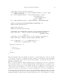
Table 1 shows how this translates into an algorithm for a generic sequence of distributions. It
is, essentially, precisely this algorithm which SMCTC allows the implementation of. However,
it should be noted that this algorithm encompasses almost all SMC algorithms.
2.2. Particle filters
The majority of SMC algorithms were developed in the context of approximate solution of
the optimal filtering and smoothing equations (although it should be noted that their use in
some areas of the physics literature dates back to at least the 1950s). Their interpretation as
SIR algorithms, and a detailed discussion of particle filtering and related fields is provided by
Journal of Statistical Software
5
At time 1
for i = 1 to N
Sample X1i ∼ q( x1 | y1 ).
ν (X1i )g( y1 |X1i )
Compute the weights w1 X1i =
and W1i ∝ w1 X1i .
q( X1i |y1 )
end for
n
o
i
Resample X1i , W1i to obtain N equally-weighted particles X 1 , N1 .
At time n ≥ 2
for i = 1 to N
i
i ← Xi
i .
,
X
Sample Xni ∼ q( xn | yn , X n−1 ) and set X1:n
1:n−1
n
i f Xi Xi
g
y
|X
(
)
(
|
)
n
n
n
n−1
.
Compute the weights Wni ∝
i
q ( Xni |yn ,Xn−1
)
end for
n
o
i
i
Resample X1:n
, Wni to obtain N equally-weighted particles X 1:n , N1 .
Table 2: SIR for particle filtering.
Doucet and Johansen (2009). Here, we attempt to present a concise overview of some of the
more important aspects of the field. Particle filtering provides a strong motivation for SMC
methods more generally and remains their primary application area at present.
General state space models (SSMs) are very popular statistical models for time series. Such
models describe the trajectory of some system of interest as an unobserved E-valued Markov
chain, known as the signal process, which for the sake of simplicity is treated as being timehomogeneous in this paper. Let X1 ∼ ν and Xn |(Xn−1 = xn−1 ) ∼ f (·|xn−1 ) and assume that
a sequence of observations, {Yn }n∈N are available. If Yn is, conditional upon Xn , independent
of the remainder of the observation and signal processes, with Yn |(Xn = xn ) ∼ g(·|xn ), then
this describes an SSM.
A common objective is the recursive approximation of an analytically intractable sequence of
posterior distributions {p ( x1:n | y1:n )}n∈N , of the form:
p(x1:n |y1:n ) ∝ ν(x1 )g(y1 |x1 )
n
Y
f (xj |xj−1 )g(yj |xj ).
(1)
j=2
There are a small number of situations in which these distributions can be obtained in closed
form (notably the linear-Gaussian case, which leads to the Kalman filter). However, in general
it is necessary to employ approximations and one of the most versatile approaches is to use
SMC to approximate these distributions. The standard approach is to use the SIR algorithm
described in the previous section, targeting this sequence of posterior distributions — although
alternative strategies exist. This leads to the algorithm described in Table 2.
We obtain, at time n, the approximation:
pb ( dx1:n | y1:n ) =
N
X
Wni δX i (dx1:n ) .
1:n
i=1
6
SMCTC: Sequential Monte Carlo in C++
Notice that, if we are interested only in approximating the marginal distributions {p (xn | y1:n )}
i
(and, perhaps, {p (y1:n )}), then we need to store only the terminal-value particles Xn−1:n
to be able to compute the weights: the algorithm’s storage requirements do not increase over
time.
Note that, although approximation of p(y1:n ) is a less-common application in the particlefiltering literature it is of some interest. It can be useful as a constituent part of other
algorithms (one notable case being the recently proposed Particle Markov Chain Monte Carlo
algorithm of Andrieu, Doucet, and Holenstein (2009)) and has direct applications in the area
of parameter estimation for SSMs. It can be calculated in an online fashion by employing the
following recursive formulation:
n
Y
p (y1:n ) = p (y1 )
p ( yk | y1:k−1 )
k=2
where p ( yk | y1:k−1 ) is given by
Z
p ( yk | y1:k−1 ) = p ( xk−1 | y1:k−1 ) f ( xk | xk−1 ) g ( yk | xk ) dxk−1:k .
Each of these conditional distributions may be interpreted
as the integral of a test function
R
ϕn (xn ) = g(yn |xn ) with respect to a distribution p(xn−1 |y1:n−1 )f (xn |xn−1 )dxn−1 which can
be approximated (at a cost uniformly bounded in time) using successive approximations to
the distributions p(xn−1 , xn |y1:n−1 ) provided by standard techniques.
2.3. SMC samplers
It has recently been established that similar techniques can be used to sample from a general
sequence of distributions defined upon general spaces (i.e. the requirement that the state
space be strictly increasing can be relaxed and the connection between sequential distributions
can be rather more general). This is achieved by applying standard SIR-type algorithms to
a sequence of synthetic distributions defined upon an increasing sequence of state spaces
constructed in such a way as to preserve the distributions of interest as their marginals.
SMC Samplers are a class of algorithms for sampling iteratively from a sequence of distributions, denoted by {πn (xn )}n∈N , defined upon a sequence of potentially arbitrary spaces,
{En }n∈N , (Del Moral et al. 2006a). The approach involves the application of SIR to a cleverly
constructed sequence of synthetic distributions which admit the distributions of interest as
marginals.
n−1
Q
The synthetic distributions are π
en (x1:n ) = πn (xn )
Lp (xp+1 , xp ) , where {Ln }n∈N is a sep=1
quence of “backward-in-time” Markov kernels from En into En−1 . With this structure, an
importance sample from π
en is obtained by taking the path x1:n−1 , an importance sample
from π
en−1 , and extending it with a Markov kernel, Kn , which acts from En−1 into En , providing samples from π
en−1 × Kn and leading to the incremental importance weight:
π
en (x1:n )
πn (xn )Ln−1 (xn , xn−1 )
=
.
(2)
π
en−1 (x1:n−1 )Kn (xn−1 , xn )
πn−1 (xn−1 )Kn (xn−1 , xn )
In most applications, each πn (xn ) can only be evaluated point-wise, up to a normalizing
constant and the importance weights defined by (2) are normalized in the same manner as in
the SIR algorithm. Resampling may then be performed.
wn (xn−1:n ) =
Journal of Statistical Software
7
The auxiliary kernels are not used directly by SMCTC as it is generally preferable to optimize the calculation of importance weights as explained in Section 4.3. However, because
they determine the form of the importance weights and influence the variance of resulting
estimators the choice of auxiliary kernels, Ln is critical to the performance of the algorithm.
As was demonstrated in Del Moral et al. (2006b) the optimal form (if resampling is used at
every iteration) is Ln−1 (xn , xn−1 ) ∝ πn−1 (xn−1 )Kn (xn−1 , xn ) but it is typically impossible to
evaluate the associated normalizing factor (which cannot be neglected as it depends upon xn
and appears in the importance weight). In practice, obtaining a good approximation to this
kernel is essential to obtaining a good estimator variance; a number of methods for doing this
have been developed in the literature.
It should also be noted that a number of other modern sampling algorithms can be interpreted
as examples of SMC samplers. Algorithms which admit such an interpretation include annealed importance sampling (Neal 2001), population Monte Carlo (Cappé, Guillin, Marin, and
Robert 2004) and the particle filter for static parameters (Chopin 2002). It is consequently
straightforward to use SMCTC to implement these classes of algorithms.
Although it is apparent that this technique is applicable to numerous statistical problems
and has been found to outperform existing techniques, including MCMC, in at least some
problems of interest (for example, see, Fan, Leslie, and Wand (2008); Johansen, Doucet, and
Davy (2008)) there have been relatively few attempts to apply these techniques. Largely, in
the opinion of the author, due to the perceived complexity of SMC approaches. Some of the
difficulties are more subtle than simple implementation issues (in particular selection of the
forward and backward kernels – an issue which is discussed at some length in the original
paper, and for which sensible techniques do exist), but we hope that this library will bring
the widespread implementation of SMC algorithms for real-world problems one step closer.
3. Using SMCTC
This section documents some practical considerations: how the library can be obtained and
what must be done in order to make use of it.
The software has been successfully compiled and tested under a number of environments
(including Gentoo, SuSe and Ubuntu Linux utilizing GCC-3 and GCC-4 and Microsoft Visual
C++ 5 under the Windows operating system). Users have also compiled the library and
example programs using devcc, the Intel C++ compiler and Sun Studio Express.
Microsoft Visual C++ project files are also provided in the msvc subdirectory of the appropriate directories and these should be used in place of the Makefile when working with
this operating system/compiler combination. The file smctc.sln in the top-level directory
comprises a Visual C++ solution which incorporates each of the individual projects.
The remainder of this section assumes that working versions of the GNU C++ compiler (g++)
except where specific reference is made to the Windows / Visual C++ combination.
In principle, other compatible compilers and makers should work although it might be necessary to make some small modifications to the Makefile or source code in some instances.
3.1. Obtaining SMCTC
SMCTC can be obtained from the author’s website (http://www2.warwick.ac.uk/fac/sci/
8
SMCTC: Sequential Monte Carlo in C++
statistics/staff/academic/johansen/smctc/ at the time of writing) and is released under
version 3 of the GNU General Public License (Free Software Foundation 2007). A link to
the latest version of the software should be present on the SMC methods preprint server
(http://www-sigproc.eng.cam.ac.uk/smc/software.html). Software is available in source
form archived in .tar, .tar.bz2 and .zip formats.
3.2. Installing SMCTC
Having downloaded and unarchived the library source (using tar xf smctc.tar or similar)
it is necessary to perform a number of operations in order to make use of the library:
1. Compile the binary component of the library.
2. Install the library somewhere in your library path.
3. Install the header files somewhere in your include path.
4. Compile the example programs to verify that everything works.
Actually, only the first of these steps is essential. The library and header files can reside
anywhere provided that the directory in which they specify is provided at compile and link
times, respectively.
Compiling the library
Enter the top level of the SMCTC directory and run make libraries. This produces a static
library named libsmctc.a and copies it to the lib directory within the SMCTC directory.
Alternatively, make all will compile the library, the documentation and the example programs. After compiling the library and any other components which are required, it is safe
to run make clean which will delete certain intermediate files.
Optional steps
After compiling the library there will be a static library named libsmctc.a within the
lib subdirectory. This should either be copied to your preferred library location (typically
/usr/local/lib on a Linux system) or its location must be specified every time the library
is used.
The header files contained within the include subdirectory should be copied to a system-wide
include directory (such as /usr/local/include) or it will be necessary to specify the location
of the SMCTC include directory whenever a file which makes use of the library is compiled.
In order to compile the examples, enter make examples in the SMCTC directory. This will
build the examples and copy them into the bin subdirectory.
Windows installation
Inevitably, some differences emerge when using the library in a Windows environment. This
section aims to provide a brief summary of the steps required to use SMCTC successfully in
this environment and to highlight the differences between the Linux and Windows cases.
Journal of Statistical Software
9
It is, of course, possible to use a make-based build environment with a command-line compiler in the Windows environment. Doing this requires minimal modification of the Linux
procedure. In order to make use of the integrated development environment provided with
Visual C++, the following steps are required.
1. Ensure that the GNU Scientific Library is installed.
2. Download and unpack smctc.zip into an appropriate folder.
3. Launch Visual Studio and open the smctc.sln that was extracted into the top-level
folder1 . This project includes project files for the library itself as well as both examples.
Note: Two configurations are available for the library as well as the examples – “Debug”
and “Release”. Be aware that the debugging version of the library is compiled with a
different name (with an appended d) to the release version: make sure that projects are
linked against the correct one.
4. If the GSL is installed in a non-standard location it may be necessary to add the appropriate include and library folders to the project files.
5. Build the library first and subsequently each of the examples.
6. Your own projects can be constructed by emulating the two examples. The key point
is to ensure that the appropriate include and library paths are specified.
3.3. Building programs with SMCTC
It should be noted that SMCTC is dependent upon the GNU Scientific Library (GSL) (Galassi
et al. 2006) for random number generation. It would be reasonably straightforward to adapt
the library to work with other random number generators but there seems to be little merit
in doing so given the provisions of the GSL and its wide availability. It is necessary, therefore,
to link executables against the GSL itself and a suitable CBLAS implementation (one is
ordinarily provided with the GSL if a locally optimized version is not available). It is necessary
to ensure that the compiler and linker include and library search paths include the directories
in which the GSL header files and libraries reside.
None of these things is likely to pose problems for a machine used for scientific software
development. Assuming that the appropriate libraries are installed, it is a simple matter of
compiling your source files with your preferred C++ compiler and then linking the resulting
object files with the SMCTC and GSL libraries. The following commands, for example, are
sufficient to compile the example program described in Section 5.1:
g++ -I../../include -c pfexample.cc pffuncs.cc
g++ pfexample.o pffuncs.o -L../../lib -lsmctc -lgsl -lgslcblas -opf
It is, of course, advisable to include some additional options to encourage the compiler to
optimize the code as much as possible once it has been debugged.
1
This is a Visual Studio 8.00 solution; due to compatibility issues it may, unfortunately, be necessary to
convert it to the version of Visual Studio you are using.
10
SMCTC: Sequential Monte Carlo in C++
3.4. Additional documentation
The library is fully documented using the Doxygen system (van Heesch 2007). This includes
a comprehensive class and function reference for the library. It can be compiled using the
command make docs in the top level directory of the library, if the freely-available Doxygen
and GraphViz (Gansner and North 2000) programs are installed. It is available compiled
from the same place as the library itself.
4. The SMCTC library
The principal rôle of this article is to introduce a C++ template class for the implementation
of quite general SMC algorithms. It seems natural to consider an object oriented approach
to this problem: a sampler itself is a single object, it contains particles and distributions;
previous generations of the sampler may themselves be viewed as objects. For convenience it
is also useful to provide an object which provides random numbers (via the GSL).
Templating is an object oriented programming (OOP) technique which abstracts the operation
being performed from the particular type of object upon which the action is carried out. One
of its simplest uses is the construction of “container classes” – such as lists – whose contents
can be of essentially any type but whose operation is not qualitatively influenced by that
type. See (Stroustrup 1991, chapter 8) for further information about templates and their use
within C++. Stroustrup (1991) helpfully suggests that, “One can think of a template as a
clever kind of macro that obeys the scope, naming and type rules of C++”.
It is natural to use such an approach for the implementation of a generic SMC library:
whatever the state space of interest, E, (and, implicitly, the distributions of interest over
those spaces) it is clear that the same actions are carried out during each iteration and the
same basic tasks need to be performed. The structure of a simple particle filter with a realvalued state space (allowing a simple double to store the state associated with a particle) or a
sophisticated trans-dimensional SMC algorithm defined over a state space which permits the
representation of complex objects of a priori unknown dimension are, essentially the same.
An SMC algorithm iteratively carries out the following steps:
ˆ Move each particle according to some transition kernel.
ˆ Weight the particles appropriately.
ˆ Resample (perhaps only if some criterion is met).
ˆ Optionally apply an MCMC move of appropriate invariant distribution. This step could
be incorporated into step 1 during the next iteration, but it is such a common technique
that it is convenient to incorporate it explicitly as an additional step.
The SMCTC library attempts to perform all operations which are related solely to the fact
that an SMC algorithm is running (iteratively moving the entire collection of particles, resampling them and calculating appropriate integrals with respect to the empirical measure associated with the particle set, for example) whilst relying upon user-defined callback functions to
perform those tasks which depend fundamentally upon the state space, target and proposal
distributions (such as proposing a move for an individual particle and weighting that particle
correctly). Whilst this means that implementing a new algorithm is not completely trivial, it
Journal of Statistical Software
sampler <T>
history <T>
11
gslrnginfo
moveset <T>
exception
rng
historyelement <T>
particle <T>
historyflags
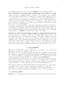
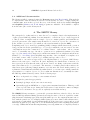
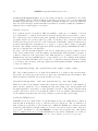
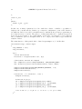
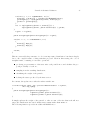
Figure 1: Collaboration diagram. T denotes the type of the sampler: The class used to
represent an element of the sample space.
provides considerable flexibility and transfers as much complexity and implementation effort
from individual algorithm implementations to the library as possible whilst preserving that
flexibility.
Although object-oriented-programming purists may prefer an approach based around derived
classes to the use of user-supplied callback functions, it seems a sensible pragmatic choice in
the present context. It has the advantage that it minimizes the amount of object-oriented
programming that the end-user has to employ (the containing programming can be written
much like C rather than C++ if the programmer is more familiar with this approach) and
simplifies the automation of as many tasks as is possible.
4.1. Library and program structure
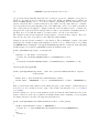
Almost the entire template library resides within the smc namespace, although a small number
of objects are defined in std to allow for simpler stream I/O in particular. Figure 1 shows the
essential structure of the library, which makes use of five templated classes and four standard
ones.
The highest level of object within the library corresponds to an entire algorithm, it is the
smc::sampler class.
smc::particle holds the value and (logarithmic, unnormalized) weight associated with an
individual sample.
smc::history describes the state of the sampler after each previous iteration (if this data is
recorded).
smc::historyelement is used by smc::history to hold the sampler state at a single earlier
iteration.
smc::historyflags contains elementary information about the history of the sampler. Presently
this is simply used to record whether resampling occurred after a particular iteration.
smc::moveset deals with the initialisation of particles, proposal distributions and additional
MCMC moves.
12
SMCTC: Sequential Monte Carlo in C++
smc:rng provides a wrapper for the GSL random number facilities. Presently only a subset
of its features are available, but direct access to the underlying GSL object is possible.
smc:gslrnginfo is used only for the handling of information about the GSL random number
generators.
smc::exception is used for error handling.
The general structure of a program (or program component) which carries out SMC using
SMCTC consists of a number of sections, regardless of the function of that program.
Initialisation Before the sampler can be used it is necessary to specify what the sampler
does and the parameters of the SMC algorithm.
Iteration Once a sampler has been created it is iterated either until completion or for one or
more iterations until some calculation or output is required. Depending upon the purpose of the software this phase, in which the sampler actually runs, may be interleaved
with the output phase.
Output If the sampler is to be of any use, it is also necessary to output either details of
the sampler itself or, more commonly, the result of calculating some expectations with
respect to the empirical measure associated with the particle set.
Section 4.2 describes how to carry out each of these phases and the remainder of this section is
then dedicated to the description of some implementation details. This section serves only to
provide a conceptual explanation of the implementation of a sampler. For detailed examples,
together with annotated source code, see Section 5.
4.2. Creating, configuring and running a sampler: smc::sampler
The top-level class is the one which most programs are going to make most use of. Indeed,
it is possible to use the SMCTC library to perform SMC with almost no direct reference
to any of its lower-level components. The first interaction between most programs and the
SMCTC library is the creation of a new sampler object. It is necessary to specify the number
of particles which the sampler will use at this stage (although some use of a variable number
of particles has been made in the literature, this is very much less common than the use of
a fixed number and for simplicity and efficiency the present library does not support such
algorithms).
The constructor of smc::sampler must be supplied with two parameters2 , the first indicates
the number of particle to use and the other must take one of two values: SMC_HISTORY_RAM
or SMC_HISTORY_NONE. If SMC_HISTORY_RAM is used then the sampler retains the full history
of the sampler in memory3 . Whilst this is convenient in some applications it uses a much
greater amount of memory and has some computational overheads; if SMC_HISTORY_NONE is
used, then only the most recent generation of particles is stored in memory. The latter setting
is to be preferred in the absence of a reason to retain historical information.
2
A more complex version of the constructor which provides control over the nature of the random number
generator used is also available; see Section 4.5 or the library documentation for details.
3
In this case, the history means the particle set as it was at every iteration in the samplers evolution. This
is different to the path-space implementation of the sampler – if one wishes to work on the path-space then it
is necessary to store the full path in the particle value.
Journal of Statistical Software
13
As the smc::sampler class is really a template class, it is necessary to specify what type
of SMC sampler is to be created. The type in this case corresponds to a class (or native
C++ type) which describes a single point in the state space of the sampler of interest. So, for
example we could create an SMC sampler suitable for performing filtering in a one-dimensional
real state space using 1000 particles and no storage of its history using the command:
smc::sampler<double> Sampler(1000, SMC_HISTORY_NONE);
or, using the C++ standard template library to provide a class of vectors, we could define a
sampler with a vector-valued real state space using 1000 particles that retains its full history
in memory using
smc::sampler<std::vector<double> > Sampler(1000, SMC_HISTORY_RAM);
Such recursive use of templates is valid although some early compilers failed to correctly
implement this feature. Note that this is the one situation in which C++ is white-spacesensitive: it is essential to close the template-type declaration with > > rather than >> for
some rather obscure reasons.
Proposals and importance weights
All of the functions which move and weight individual particles are supplied to the
smc::sampler object via an object of class smc::moveset. See Section 4.3 for details. Once an
smc::moveset object has been created, it is supplied to the smc::sampler via the SetMoveSet
member function. This function takes a single argument which should be an already initialized
smc::moveset object which specifies functions used for moving and weighting particles.
Once the moveset has been specified, the sampler will call these functions as needed with no
further intervention from the user.
Resampling
A number of resampling schemes are implemented within the library. Resampling can be
carried out always, never or whenever the effective sample size (ESS) in the sense of (Liu
2001, p. 35–36) falls below a specified threshold.
To control resampling behaviour, use the SetResampleParams(ResampleType, double) member function. The first argument should be set to one of the values allowed by ResampleType
enumeration indicating the resampling scheme to use (see Table 3) and the second controls
when resampling is performed. If the second argument is negative, then resampling is never
performed; if it lies in [0, 1] then resampling is performed when the ESS falls below that
proportion of the number of particles and when it is greater than 1, resampling is carried out
when the ESS falls below that value. Note that if the second parameter is larger than the
total number of particles, then resampling will always be performed.
The default behaviour is to perform stratified resampling whenever the ESS falls below half
the number of particles. If this is acceptable then no call of SetResampleParams is required,
although such a call can improve the readability of the code.
MCMC Diversification
Following the lead of the resample-move algorithm (Gilks and Berzuini 2001), many users of
SMC methods make use of an MCMC kernel of the appropriate invariant distribution after
the resampling step. This is done automatically by SMCTC if the appropriate component
14
SMCTC: Sequential Monte Carlo in C++
Value
SMC_RESAMPLE_MULTINOMIAL
SMC_RESAMPLE_RESIDUAL
SMC_RESAMPLE_STRATIFIED
SMC_RESAMPLE_SYSTEMATIC
Resampling scheme used
Multinomial
Residual (Liu and Chen 1998)
Stratified (Carpenter, Clifford, and Fearnhead 1999)
Systematic (Kitagawa 1996)
Table 3: Enumeration defined in sampler.hh which can be used to specify a resampling
scheme.
of the moveset supplied to the sampler was non-null. See Section 5.2 for an example of an
algorithm with such a move.
Running the algorithm
Having set all of the algorithm’s operating parameters – including the smc::moveset; it is not
possible to initialize the sampler before the sampler has been supplied with a function which
it can initialize the particles with – the first step is to initialize the particle system. This is
done using the Initialise method of the smc::sampler which takes no arguments. This
function eliminates any information from a previous run of the sampler and then initializes
all of the particles by calling the function specified in the moveset once for each of them.
Once the particle system has been initialized, one may wish to output some information
from the first generation of the system (see the following section). It is then time to begin
iterating the particle system. The sampler class provides two methods for doing this: one
which should be used if the program must control the rate of execution (such as in a realtime environment) or to interact with the sampler each iteration (perhaps obtaining the next
observation for the likelihood function and calculating estimates of the current state) and
another which is appropriate if one is interested in only the final state of the sampler. The
first of these is Iterate() and it takes no arguments: it simply propagates the system to the
next iteration using the moves specified in the moveset, resampling if the specified resampling
criterion is met. The other, IterateUntil(int) takes a single argument: the number of the
iteration which should be reached before the sampler stops iterating. The second function
essentially calls the first iteratively until the desired iteration is reached.
Output
The smc::sampler object also provides the interface by which it is possible to perform some
basic integration with respect to empirical measures associated with the particle set and to
obtain the locations and weights of the particles.
Simple integration The most common use for the weighted sample associated with an
SMC algorithm is the approximation of expectations with respect to the target measure. The
Integrate function performs the appropriate calculation (for a user-specified function) and
returns the estimate of the integral.
In order to use the built-in sample integrator, it is necessary to provide a function which
can be evaluated for each particle. The library then takes care of calculating the appropriate
weighted sum over the particle set. The function, here named integrand, should take the
Journal of Statistical Software
15
form:
double integrand(const T& , void *)
where T denotes the type of the smc::sampler template class in use. This function will be
called with the first argument set to (a constant reference to) the value associated with each
particle in turn by the smc::sampler class. The function has an additional argument of type
void * to allow the user to pass arbitrary additional information to the function.
Having defined such a function, its integral with respect to the weighted empirical measure
associated with the particle set associated with an smc::sampler object named Sampler is
provided by calling
Sampler.Integrate(integrand, void *(p));
where p is a pointer to auxiliary information that is passed directly to the integrand function
via its second argument – this may be safely set to NULL if no such information is required
by the function. See example 5.1 for examples of the use of this function with and without
auxiliary information.
Path-sampling integration As is described in Section 5.2 it is sometimes useful to estimate the normalizing constant of the final distribution using a joint Monte Carlo/numerical
integration of the path-sampling identity of Gelman and Meng (1998). The IntegratePS
performs this task, again using a user-specified function. This function can only be used if
the sampler was created with the SMC_HISTORY_RAM option as it makes use of the full history
of the particle set.
The function to be integrated may have an explicit dependence upon the generation of the
sampler and so an additional argument is supplied to the function which is to be integrated.
In this case, the function (here named integrand_ps) should take the form:
double integrand_ps(long, const T& , void *)
Here, the first argument corresponds to the iteration number which is passed to the function explicitly and the remaining arguments have the same interpretation as in the simple
integration case.
An additional function is also required: one which specifies how far apart successive distributions are – this information is required to calculate the trapezoidal integral used in the path
sampling approximation. This function, here termed width_ps, takes the form
double width_ps(long, void *)
where the first argument is set to an iteration time and the second to user-supplied auxiliary
information. It should return the width of the bin of the trapezoidal integration in which the
function is approximated by the specified generation.
Once these functions have been defined, the full path sampling calculation is calculated by
calling
Sampler.IntegratePS(integrand_ps, width_ps, void *(p));
where p is a pointer to auxiliary information that is passed directly to the integrand_ps
function via its third argument – this may be safely set to NULL if no such information is
required by the function. Section 5.2 provides an example of the use of the path-sampling
integrator.
16
SMCTC: Sequential Monte Carlo in C++
General output For more general tasks it is possible to access the locations and weights
of the particles directly.
Three low-level member functions provide access to the current generation of particles, each
takes a single integer argument corresponding to a particle index. The functions are
GetParticleValue(int n)
GetParticleLogWeight(int n)
GetParticleWeight(int n)
and they return a constant reference to the value of particle n, the logarithm of the unnormalized weight of particle n and the unnormalized weight of that particle, respectively.
The GetHistory() member of the smc::sampler class returns a constant pointer to the
smc::history class in which the full particle history is stored to allow for very general use
of the generated samples. This function is used in much the same manner as the simple
particle-access functions described above; see the user manual for detailed information.
Finally, a human-readable summary of the state of the particle system can be directed to an
output stream using the usual << operator.
4.3. Specifying proposals and importance weights: smc::moveset
It is necessary to provide SMCTC with functions to initialize a particle; move a particle at
each iteration and weight it appropriately and, if MCMC moves are required, then a function
to apply such a move to a particle is needed. The following sections describe the functions
which must be supplied for each of these tasks and this section concludes with a discussion
of how to package these functions into an smc::moveset object and to pass the object to the
sampler.
Initializing the particles
The first thing that the user needs to tell the library how to do is to initialize an individual
particle: how should the initial value and weight be set?
This is done via an initialisation function which should have prototype:
smc::particle<T> fInitialise(smc::rng *pRng);
where T denotes the type of the sampler and the function is here named fInitialise.
When the sampler calls this function, it supplies a pointer to an smc::rng class which serves
as a source of random numbers (the user is, of course, free to use an alternative source if
they prefer) which can be accessed via member functions in that class which act as wrappers
to some of the more commonly-used of the GSL random variate generators or by using the
GetRaw() member function which returns a pointer to the underlying GSL random number
generator. Note that the GSL contains a very large number of efficient generators for random
variables with most standard distributions.
The function is expected to produce a new smc::particle of type T and to return this object
to the sampler. The simplest way to do this is to use the initializing-constructor defined for
smc::particle objects. If an object, value of type T and a double named dLogWeight are
available then
Journal of Statistical Software
17
smc::particle<T> (value, dLogWeight)
will produce a new particle object which contains those values.
Moving and weighting the particles
Similarly, it is necessary for a proposal function to be supplied. Such a function follows broadly
the same pattern as the initialisation function but is supplied with the existing particle value
and weight (which should be updated in place), the current iteration number and a pointer
to an smc::rng class which serves as a source of randomness.
The proposal function(s) take the form:
void fMove(long, smc::particle<T> &, smc::rng *)
When the sampler calls this function, the first argument is set to the current iteration number,
the second to an smc::particle object which corresponds to the particle to be updated (this
should be amended in place and so the function need return nothing) and the final argument
is the random number generator.
There are a number of functions which can be used to determine the current value and weight
of the particle in question and to alter their values. It is important to remember that the
weight must be updated as well as the particle value. Whilst this may seem undesirable,
and one may ask why the library cannot simply calculate the weight automatically from
supplied functions which specify the target distributions, proposal densities (and auxiliary
kernel densities, where appropriate), there is a good reason for this. The automatic calculation
of weights from generic expressions has two principal drawbacks: it need not be numerically
stable if the distributions are defined on spaces of high dimension (it is likely to correspond
to the ratio of two very small numbers) and, it is very rarely an efficient way to update
the weights. One should always eliminate any cancelling terms from the numerator and
denominator as well as any constant (independent of particle value) multipliers in order to
minimize redundant calculations. Note that the sampler assumes that the weights supplied are
not normalized; no advantage is obtained by normalizing them (this also allows the sampler
to renormalize the weights as necessary to obtain numerical stability).
Changing the value There are two approaches to accessing and changing the value of
the particle. The first is to use the GetValue() and SetValue(T) (where T, again serves as
shorthand for the type of the sampler) functions to retrieve and then set the value. This is
likely to be satisfactory when dealing with simple objects and produces safe, readable code.
The alternative, which is likely to produce substantially faster code when T is a complicated
class, is to use the GetValuePointer() function which returns a pointer to the internal
representation of the particle value. This pointer can be used to modify the value in place to
minimize the computational overhead.
Updating the weight The present unnormalized weight of the particle can be obtained
with the GetWeight() method; its logarithm with GetLogWeight(). The SetWeight(double)
and SetLogWeight(double) functions serve to change the value. As one generally wishes to
multiply the weight by the current incremental weight the functions AddToLogWeight(double)
18
SMCTC: Sequential Monte Carlo in C++
and MultiplyWeightBy(double) are provided and perform the obvious function. Note that
the logarithmic version of all these functions should be preferred for two reasons: numerical
stability is typically improved by working with logarithms (weights are often very small and
have an enormous range) and the internal representation of particle weights is logarithmic so
using the direct forms requires a conversion.
Mixtures of moves
It is common practice in advanced SMC algorithms to make use of a mixture of several
proposal kernels. So common, in fact, that a dedicated interface has been provided to remove
the overhead associated with selecting and applying an individual move from application
programs. If there are several possible proposals, one should produce a function of the form
described in the previous section for each of them and, additionally, a function which selects
(possibly randomly) the particular move to apply to a given particle during a particular
iteration. The sampler can then apply these functions appropriately, minimizing the risk of
any error being introduced at this stage.
In order to use the automated mixture of moves, two additional objects are required. One is
a list of move functions in a form the sampler can understand. This amounts to an array of
pointers to functions of the appropriate form. Although the C++ syntax for such objects is
slightly messy, it is very straightforward to create such an object. For example, if the sampler
is of type T and fMv1 and fMv2 each correspond to a valid move function then the following
code would produce an array of the appropriate type named pfMoves which contains pointers
to these two functions:
void (*pfMoves[])(long, smc::particle<T> &,smc::rng*) = {fMv1, fMv2};
The other required function is one that selects which move to make at any given moment.
In general, one would expect the selection to have some randomness associated with it. The
function which performs the selection should have prototype:
long fSelect(long lTime, const smc::particle<T> & p, smc::rng *pRng)
When it is called by the sampler, lTime will contain the current iteration of the sampler, p
will be an smc::particle object containing the state and weight of the current particle and
the final argument corresponds to a random number generator. The function should return
a value between zero and one below than the number of moves available (this is interpreted
by the sampler as an index into the array of function pointers defined previously).
Additional MCMC moves
If MCMC moves are required then one should simply produce an additional move function
with an almost identical prototype to that used for proposal moves. The one difference is
that normal proposals have a void return type, whilst the MCMC move function should
return int. The function should return zero if a move is rejected and a positive value if it
is accepted4 . In addition to allowing SMCTC to monitor the acceptance rate, this ensures
that no confusion between proposal and MCMC moves is possible. Ordinarily, one would not
4
It is advisable to return a positive value in the case of moves which do not involve a rejection step.
Journal of Statistical Software
19
expect these functions to alter the weight of the particle which they move but this is not
enforced by the library.
Creating an smc::moveset object
Having specified all of the individual functions, it is necessary to package them all into a
moveset object and then tell the sampler to use that moveset.
The simplest way to fill a moveset is to use an appropriate constructor. There is a threeargument form which is appropriate for samplers with a single proposal function and a fiveargument variant for samplers with a mixture of proposals.
Single-proposal movesets If there is a single proposal, then the moveset must contain
three things: a pointer to the initialisation function, a pointer to the proposal function and,
optionally, a pointer to an MCMC move function (if one is not required, then the argument
specifying this function should be set to NULL). A constructor which takes three arguments
exists and has prototype
moveset ( particle<T>(*pfInit)(rng *),
void(*pfNewMoves)(long, particle<T> &, rng *),
int(*pfNewMCMC)(long, particle<T> &, rng *))
indicating that the first argument should correspond to a pointer to the initialisation function,
the second to the move function and the third to any MCMC function which is to be used
(or NULL). Section 5.1 shows this approach in action.
Mixture-proposal movesets There is also a constructor which initializes a moveset for
use in the mixture-formulation. Its prototype takes the form:
moveset ( particle<T>(*pfInit)(rng *),
long(*pfMoveSelector)(long, const particle<T> &, rng *),
long nMoves,
void(**pfNewMoves)(long, particle<T> &, rng *),
int(*pfNewMCMC)(long, particle<T> &, rng *))
Here, the first and last arguments coincide with those of the single-proposal-moveset constructor described above; the second argument is the function which selects a move, the second
is the number of different moves which exist and the fourth argument is an array of nMoves
pointers to move functions. This is used in Section 5.2.
Using a moveset Having created a moveset by either of these methods, all that remains
is to call the SetMoveSet member of the sampler, specifying the newly-created moveset as
the sole argument. This tells the sampler object that this moveset contains all information
about initialisation, proposals, weighting and MCMC moves and that calling the appropriate members of this object will perform the low-level application-specific functions which it
requires the user to specify.
20
SMCTC: Sequential Monte Carlo in C++
4.4. Error handling: smc::exception
If an error that is too serious to be indicated via the return value of a function within the
library occurs then an exception is thrown.
Exceptions indicating an error within SMCTC are of type smc::exception. This class contains four pieces of information:
const char* szFile;
long lLine;
long lCode;
const char* szMessage;
szFile is a NULL-terminated string specifying the source file in which the exception occurred;
lLine indicates the line of that file at which the exception was generated. lCode provides a
numerical indication of the type of error (this should correspond to one of the SMCX_* constants
defined in smc-exception.hh) and, finally, szMessage provides a human-readable description
of the problem which occurred. For convenience, the << operator has been overloaded so that
os << e will send a human-readable description of the smc::exception, e to an ostream,
os – see Section 5.1 for an example.
4.5. Random number generation
In principle, no user involvement is required to configure the random number generation used
by the SMCTC library. However, if no information is provided then the sampler will use the
same pseudorandom number sequence for every execution: it simply uses the GSL default
generator type and seed. In fact, complete programmatic control of the random number
generator can be arranged via the random number generator classes (it is possible to supply
one to the smc::sampler class when it is created rather than allowing it to generate a default).
However, this is not an essential feature of the library, the details can be found in the class
reference and are not reproduced here.
For day-to-day use, it is probably sufficient for most users to take advantage of the fact that, as
invoked by SMCTC’s default behaviour, GSL checks two environment variables before using
its default generator. Consequently, it is possible to control the behaviour of the random
number sequence provided to any program which uses the SMCTC library by setting these
environment variables before launching the program. Specifically, GSL_RNG_SEED specifies
the random number seed and GSL_RNG_TYPE specifies which generator should be used – see
Galassi et al. (2006) for details.
By way of an example, the pf binary produced by compiling the example in Section 5.1 can
be executed using the “ranlux” generator with a seed of 36532673278 by entering the following
at a BASH (Bourne Again Shell) prompt from the appropriate directory:
GSL_RNG_TYPE=ranlux GSL_RNG_SEED=36532673278 ./pf
5. Examples applications
This section provides two sample implementations: a simple particle filter in Section 5.1 and
a more involved SMC sampler which estimates rare event probabilities in Section 5.2. This
Journal of Statistical Software
21
section shows how one can go about implementing SMC algorithms using the SMCTC library
and (hopefully) emphasizes that no great technical requirements are imposed by the use of
a compiled language such as C++ in the development of software of this nature. It is also
possible to use these programs as a basis for the development of new algorithms.
5.1. A simple particle filter
Model
It is useful to look at a basic particle filter in order to see how the description above relates to
a real implementation. The following simple state space model, known as the almost constant
velocity model in the tracking literature, provides a simple scenario.
The state vector Xn contains the position and velocity of an object moving in a plane: Xn =
(sxn , uxn , syn , uyn ). Imperfect observation of the position, but not velocity, is possible at each
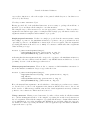
time instance. The state and observation equations are linear with additive noise:
Xn = AXn−1 + Vn
Yn = BXn + αWn
where


1 ∆ 0 0
 0 1 0 0 

A=
 0 0 1 ∆ 
0 0 0 1
B=
1 0 0 0
0 0 1 0
α = 0.1,
and we assume that the elements of the noise vector Vn are independent normal with variances
0.02 and 0.001 for position and velocity components, respectively. The observation noise,
Wn , comprise independent, identically distributed t-distributed random variables with ν = 10
degrees of freedom. The prior at time 0 corresponds to an axis-aligned Gaussian with variance
4 for the position coordinates and 1 for the velocity coordinates.
Implementation
For simplicity, we define a simple bootstrap filter (Gordon, Salmond, and Smith 1993) which
samples from the system dynamics (i.e. the conditional prior of a given state variable given
the state at the previous time but no knowledge of any subsequent observations) and weights
according to the likelihood.
The pffuncs.hh header performs some basic housekeeping, with function prototypes and
global-variable declarations. The only significant content is the definition of the classes used
to describe the states and observations:
class cv_state
{
public:
double x_pos, y_pos;
double x_vel, y_vel;
22
SMCTC: Sequential Monte Carlo in C++
};
class cv_obs
{
public:
double x_pos, y_pos;
};
In this case, nothing sophisticated is done with these classes: a shallow copy suffices to
duplicate the contents and the default copy constructor, assignment operator and destructor
are sufficient. Indeed, it would be straightforward to implement the present program using no
more than an array of doubles. The purpose of this (apparently more complicated) approach
is twofold: it is preferable to use a class which corresponds to precisely the objects of interest
and, it illustrates just how straightforward it is to employ user-defined types within the
template classes.
The main function of this particle filter, defined in pfexample.cc, looks like this:
int main(int argc, char** argv)
{
long lNumber = 1000;
long lIterates;
try {
//Load observations
lIterates = load_data("data.csv", &y);
//Initialize and run the sampler
smc::sampler<cv_state> Sampler(lNumber, SMC_HISTORY_NONE);
smc::moveset<cv_state> Moveset(fInitialise, fMove, NULL);
Sampler.SetResampleParams(SMC_RESAMPLE_RESIDUAL, 0.5);
Sampler.SetMoveSet(Moveset);
Sampler.Initialise();
for(int n=1 ; n < lIterates ; ++n) {
Sampler.Iterate();
double xm,xv,ym,yv;
xm = Sampler.Integrate(integrand_mean_x,NULL);
xv = Sampler.Integrate(integrand_var_x, (void*)&xm);
ym = Sampler.Integrate(integrand_mean_y,NULL);
yv = Sampler.Integrate(integrand_var_y, (void*)&ym);
cout << xm << "," << ym << "," << xv << "," << yv << endl;
}
}
Journal of Statistical Software
catch(smc::exception
{
cerr << e;
exit(e.lCode);
}
23
e)
}
This should be fairly self-explanatory, but some comments are justified. The call to LoadData
serves to load some observations from disk (the LoadData function is included in the source
file but is not detailed here as it could be replaced by any method for sourcing data; indeed,
in real filtering applications one would anticipate this data arriving in real time from a signal
source). This function assumes that a file called Data.csv exists in the present directory; the
first line of this file identifies the number of observation pairs present and the remainder of
the file contains these observations in a comma-separated form. A suitable data file is present
in the downloadable source archive.
It should be noted that some thought may be needed to develop sensible data-handling strategies in complex applications. It may be preferable to avoid the use of global variables by employing singleton data sources or otherwise implementing functions which return references
to a current data-object. This problem is likely to be application specific and is not discussed
further here.
The body of the program is enclosed in a try block so that any exceptions thrown by the
sampler can be caught, allowing the program to exit gracefully and display a suitable error
message should this happen. The final lines perform this elementary error handing.
Within the try block, the program creates an smc::sampler which employs lNumber= 1000
particles and which does not store the history of the system. After which it creates an
smc::moveset comprising an initialisation function fInitialise and a proposal function
fMove – the final argument is NULL as no additional MCMC moves are used. These functions
are described below.
Once the basic objects have been created, the program initialize the sampler by:
ˆ Specifying that we wish to perform residual resampling when the ESS drops below 50%
of the number of particles.
ˆ Supplying the moveset-information to the sampler.
ˆ Telling the sampler to initialize itself and all of the particles (the fInitialise function
is called for each particle at this stage).
The for structure which follows iterates through the observations, propagating the particle
set from one filtering distribution to the next and outputting the mean and variance of sxn
and syn for each n. Within every iteration, the sampler is called upon to predict and update
the particle set, resampling if the specified condition is met. The remaining lines calculate
the mean and variance of the x and y coordinates using the simple integrator built in to the
sampler.
Consider the x components (the y components are dealt with in precisely the same way with
essentially identical code). The mean is calculated by the line which asks the sampler to obtain
the weighted average of function integrand_mean_x over the particle set. This function, as
we require the mean of sxn , simply returns the value of sxn for the specified particle:
24
SMCTC: Sequential Monte Carlo in C++
double integrand_mean_x(const cv_state& s, void *)
{
return s.x_pos;
}
The following line then calculates the variance. Whilst it would be straightforward to estimate
the mean of (sxn )2 using the same method as sxn and to calculate the variance from this, an
alternative is to supply the estimated mean to a function which returns the squared difference
between sxn and an estimate of its mean. We take this approach to illustrate the use of the
final argument of the integrand function. The function, in this case is:
double integrand_var_x(const cv_state& s, void* vmx)
{
double* dmx = (double*)vmx;
double d = (s.x_pos - (*dmx));
return d*d;
}
as the final argument of the Sampler.Integrate() call is set to a pointer to the mean of sxn
estimated previously, this is what is supplied as the final argument of the integrand function
when it is called for each individual particle.
The functions used by the particle filter are contained in pffuncs.cc. The first of these is
the initialisation function:
smc::particle<cv_state> fInitialise(smc::rng *pRng)
{
cv_state value;
value.x_pos
value.y_pos
value.x_vel
value.y_vel
=
=
=
=
pRng->Normal(0,sqrt(var_s0));
pRng->Normal(0,sqrt(var_s0));
pRng->Normal(0,sqrt(var_u0));
pRng->Normal(0,sqrt(var_u0));
return smc::particle<cv_state>(value,logLikelihood(0,value));
}
This code block declares an object of the same type as the value of the particle, use the
SMCTC random number class to initialize the position and velocity components of the state
to samples from appropriate independent Gaussian distributions and then, as the particle has
been drawn from a distribution corresponding to the prior distribution at time 0, it is simply
weighted by the likelihood. The final returns an smc::particle object with the value of
value and a weight obtained by calling the logLikelihood function with the first argument
set to the current iteration number and the second to value.
The logLikelihood function
double logLikelihood(long lTime, const cv_state & X)
{
Journal of Statistical Software
25
return - 0.5 * (nu_y + 1.0) *
(log(1 + pow((X.x_pos - y[lTime].x_pos)/scale_y,2) / nu_y)
+ log(1 + pow((X.y_pos - y[lTime].y_pos)/scale_y,2) / nu_y));
}
is slightly misnamed. It does not return the log likelihood, but the log of the likelihood up
to a normalizing constants. Its operation is not significantly more complicated than it would
be if the same function were implemented in a dedicated statistical language.
Finally, the move function takes the form:
void fMove(long lTime, smc::particle<cv_state > & pFrom, smc::rng *pRng)
{
cv_state * cv_to = pFrom.GetValuePointer();
cv_to->x_pos
cv_to->x_vel
cv_to->y_pos
cv_to->y_vel
+=
+=
+=
+=
cv_to->x_vel * Delta + pRng->Normal(0,sqrt(var_s));
pRng->Normal(0,sqrt(var_u));
cv_to->y_vel * Delta + pRng->Normal(0,sqrt(var_s));
pRng->Normal(0,sqrt(var_u));
pFrom.AddToLogWeight(logLikelihood(lTime, *cv_to));
}
Again, this is reasonably straightforward. It commences by obtaining a pointer to the value
associated with the particle so that it can be modified in place. It then adds appropriate
Gaussian random variables to each element of the state, according to the system dynamics,
using the SMCTC random number class. Finally, the value of the log likelihood is added to
the logarithmic weight of the particle (this, of course, is equivalent to multiplying the weight
by the likelihood).
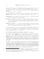
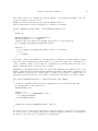
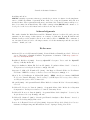
Between them, these functions comprise a complete working particle filter. In total, 156
lines of code and 28 lines of header file are involved in this example program – including
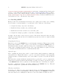
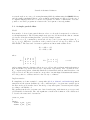
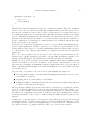
significant comments and white-space. Figure 2 shows the output of this algorithm running
on simulated data, together with the simulated data itself and the observations. Only the
position coordinates are illustrated. For reference, using a 1.7 GHz Pentium-M, this simulation
takes 0.35 s to run for 100 iterations using 1000 particles.
5.2. Gaussian tail probabilities
The following example is an implementation of an algorithm, described in (Johansen, Del
Moral, and Doucet 2006, Section 2.3.1), for the estimation of rare event probabilities. A
detailed discussion is outside the scope of this paper.
Model and distribution sequence
In general, estimating the probability of rare events (by definition, those with very small
probability) is a difficult problem. In this section we consider one particular class of rare
events. We are given a (possibly inhomogeneous) Markov chain, (Xn )n∈N , which takes its
26
SMCTC: Sequential Monte Carlo in C++
14
Ground Truth
Filtering Estimate
Observations
12
10
8
6
4
2
-7
-6
-5
-4
-3
-2
-1
Figure 2: Proof of concept: Simulated data, observations and the posterior mean filtering
estimates obtained by the particle filter.
values in a sequence of measurable spaces (En )n∈N with initial distribution η0 and elementary
transitions given by the set of Markov kernels (Mn )n≥1 .
The law P of the Markov chain is defined by its finite dimensional distributions:
−1
P ◦ X0:N
(dx0:N ) = η0 (dx0 )
N
Y
Mi (xi−1 , dxi ).
(3)
i=1
For this Markov chain, we wish to estimate the probability of the path of the chain lying
in some “rare” set, R, over some deterministic interval 0 : P . We also wish to estimate the
distribution of the Markov chain conditioned upon the chain lying in that set, i.e., to obtain
a set of samples from the distribution:
−1
Pη0 ◦ X0:P
(·|X0:P ∈ R) .
(4)
In general, even if it is possible to sample directly from η0 (·) and from Mn (xn−1 , ·) for all n and
almost all xn−1 it is difficult to estimate either the probability or the conditional distribution.
Journal of Statistical Software
27
The proposed approach is to employ a sequence of intermediate distributions which move
−1
−1
smoothly from P ◦ X0:P
to the target distribution P ◦ X0:P
(·|X0:P ∈ R) and to obtain samples
from these distributions using SMC methods. By operating directly upon the path space, we
obtain a number of advantages. It provides more flexibility in constructing the importance
distribution than methods which consider only the time marginals, and allows us to take
complex correlations into account.
We can, of course, cast the probability of interest as the expectation of an indicator function
over the rare set, and the conditional distribution of interest in a similar form as:
P (X0:P ∈ R) = E [IR (X0:P )] ,
P (dx0:p ∩ R)
.
P (dx0:p |X0:P ∈ R ) =
E [IR (X0:P )]
We concern ourselves with those cases in which the rare set of interest can be characterized
by some measurable function, V : E0:P → R, which has the properties that:
V :
R
→ [V̂ , ∞),
V : E0:P \ R → (−∞, V̂ ).
In this case, it makes sense to consider a sequence of distributions defined by a potential
function which is proportional to their Radon-Nikodým derivative with respect to the law of
the Markov chain, namely:
gθ (x0:p ) =
−1
1 + exp −α(θ) V (x0:P ) − V̂
where α(θ) : [0, 1] → R+ is a differentiable monotonically-increasing function such that α(0) =
0 and α(1) is sufficiently large that this potential function approaches the indicator function
on the rare set as we move through the sequence of distributions defined by this potential
function at the parameter values θ ∈ {t/T : t ∈ {0, 1, . . . , T }}.
T
Let πt (dx0:P ) ∝ P(dx0:P )gt/T (x0:P ) t=0 be the sequence of distributions which we use. The
SMC samplers framework allows us to obtain a set of samples from each of these distributions
in turn via a sequential importance sampling and resampling strategy. Note that each of
these distributions is over the first P + 1 elements of a Markov chain: they are defined upon
a common space.
In order to estimate the expectation which we seek, make use of the identity:
Z1
EP [IR (X0:P )] = EπT
IR (X0:P ) ,
g1 (X0:P )
R
where Zθ = gθ (xo:P )P(dx0:P ) and use the particle approximation of the right hand side of
this expression. This is simply importance sampling: Z1 /g1 (·) is simply the density of π0 with
respect to πT and we wish to estimate the expectation of this indicator function under π0 .
Similarly, the subset of particles representing samples from πT which hit the rare set can be
interpreted as (weighted) samples from the conditional distribution of interest.
(i,j)
We use the notation (Yti )N
to describe the j th
i=1 to describe the particle set at time t and Yt
(i,−p)
state in the Markov chain described by particle i at time t. We further use Yt
to refer to
28
SMCTC: Sequential Monte Carlo in C++
th
every state in the
Markov chain described
by particle i at time t except the p , and similarly,
(i,−p)
(i,0:p−1)
(i,p+1:P )
Yt
∪ Y 0 , Yt
, Y 0 , Yt
, i.e., it refers to the Markov chain described by the
same particle, with the pth state of the Markov chain replaced by some quantity Y 0 .
The path-sampling approximation
The estimation of the normalizing constant associated with our potential function can be
achieved by a Monte Carlo approximation of the path sampling formulation given by Gelman
and Meng (1998). Given a parameter θ such that a potential function gθ (x) allows a smooth
transition from a reference distribution to a distribution of interest, as some parameter increases from zero to one, one can estimate the logarithm of the ratio of their normalizing
constants via the integral relationship:
Z 1 Z1
dgθ
=
Eθ
dθ,
(5)
log
Z0
dθ
0
where Eθ denotes the expectation under πθ .
In our cases, we can describe our sequence of distributions in precisely this form via a discrete
sequence of intermediate distributions parametrized by a sequence of values of θ:
d log gθ
(V (x) − V̂ )
dα
(x) =
dθ
exp(α(θ)(V (x) − V̂ )) + 1 dθ
#
"
Z t/T
Zt/T
dα
(V (·) − V̂ )
dθ
⇒ log
=
Eθ
Z0
exp(α(θ)(V (·) − V̂ )) + 1 dθ
0
#
"
Z α(t/T )
(V (·) − V̂ )
=
E α(t/T )
dα,
α(1)
exp(α(V (·) − V̂ )) + 1
0
where Eθ is used to denote the expectation under the distribution associated with the potential
function at the specified value of its parameter.
The SMC sampler provides us with a set of weighted particles obtained from a sequence of
distributions suitable for approximating the integrals in (5). At each αt we can obtain an
estimate of the expectation within the integral via the usual importance sampling estimator;
and the integral over θ (which is one dimensional and over a bounded interval) can then be
approximated via a trapezoidal integration. As we know that Z0 = 0.5 we are then able
to estimate the normalizing constant of the final distribution and then use an importance
sampling estimator to obtain the probability of hitting the rare set.
A Gaussian case
It is useful to consider a simple example for which it is possible to obtain analytic results
for the rare event probability. The tails of a Gaussian distribution serve well in this context,
and we borrow the example of Del Moral and Garnier (2005). We consider a homogeneous
Markov chain defined on (R, B(R)) for which the initial distribution is a standard Gaussian
distribution and each kernel is a standard Gaussian distribution centred on the previous
position:
η0 (dx) = N (dx; 0, 1) ∀n > 0 : Mn (x, dy) = N (dy; x, 1).
Journal of Statistical Software
29
The function V (x0:P ) := xP corresponds to a canonical coordinate operator and the rare set
R := E P × [V̂ , ∞) is simply a Gaussian tail probability: the marginal distribution of XP is
simply N (0, P + 1) as XP is the sum of P + 1 iid standard Gaussian random variables.
Sampling from π0 is trivial. We employ an importance kernel which moves position i of the
chain by ijδ. j is sampled from a discrete distribution. This distribution over j is obtained
by considering a finite collection of possible moves and evaluating the density of the target
distribution after each possible move. j is then sampled from a distribution proportional
to this vector of probabilities. δ is an arbitrary scale parameter. The operator, Gε , defined
P
(i,p)
, where ε is interpreted as a parameter, is used for notational
by Gε Yni = Yn + pε
p=0
convenience.
This forward kernel can be written as:
i
Kn (Yn−1
, Yni ) =
S
X
i
ωn (Yn−1
, Yni )δGδj Y i (Yni ),
n−1
j=−S
where the probability of each of the possible moves is given by
i
ωn (Yn−1
, Yni ) =
πn (Yni )
PS
i
j=−S πn (Gδj Yn−1 )
.
This leads to the following optimal auxiliary kernel:
i )
πn−1 (Yn−1
i
Ln−1 (Yni , Yn−1
) =
S
P
S
P
j=−S
i
i , Y i )δ
ωn (Yn−1
n Gδj Y i (Yn )
n−1
.
πn−1 (G−δj Yni )ωn (G−δj Yni , Yn )
j=−S
The incremental importance weight is consequently:
i
wn (Yn−1
, Yni ) =
πn (Yni )
S
P
j=−S
.
πn (G−δj Yni )wn (G−δj Yni , Yni )δGδj Y i (Yni )
n−1
As the calculation of the integrals involved in the incremental weight expression tend to be
analytically intractable in general, we have made use of a discrete grid of proposal distributions
as proposed by Peters (2005). This naturally impedes the exploration of the sample space.
Consequently, we make use of a Metropolis-Hastings kernel of the correct invariant distribution
at each time step (whether resampling has occurred, in which case this also helps to prevent
sample impoverishment, or not). We make use of a linear schedule α(θ) = kθ and show the
results of our approach (using a chain of length 15, a grid spacing of δ = 0.025 and S = 12 in
the sampling kernel) in Table 4.
It should be noted that constructing a proposal in this way has a number of positive points: it
allows the use of a (discrete approximation to) essentially any proposal distribution, and it is
possible to use the optimal auxiliary kernel with it. However, there are also some drawbacks
and we would not recommend the use of this strategy without careful consideration. In
particular, the use of a discrete grid limits the movement which is possible considerably and
30
SMCTC: Sequential Monte Carlo in C++
Threshold, V̂
5
10
15
20
25
30
√
9 √15
10 15
True log probability
-2.32
-5.32
-9.83
-15.93
-23.64
-33.00
-43.63
-53.23
SMC mean
-2.30
-5.30
-9.81
-15.94
-23.83
-33.08
-43.61
-53.20
SMC variance
0.016
0.028
0.026
0.113
0.059
0.106
0.133
0.142
k
2
4
6
10
12.5
14
12
11.5
T
333
667
1000
2000
2500
3500
3600
4000
Table 4: Means and variances of the estimates produced by 10 runs of the proposed algorithm
using 100 particles at each threshold value for the Gaussian random walk example.
it will generally be necessary to make use of accompanying MCMC moves to maintain sample
diversity. More seriously, these grid-type proposals are typically extremely expensive to use
as they require numerous evaluations of the target distribution for each proposal. Although
it provides a more-or-less automatic mechanism for constructing a proposal and using its
optimal auxiliary kernel, the cost of each sample obtained in this way can be sufficiently high
that using a simpler proposal kernel with an approximation to its optimal auxiliary kernel
could yield rather better performance at a given computational cost.
Implementation
The simfunctions.hh file in this case contains the usual overhead of function prototypes and
global variable definitions. It also includes a file markovchain.h which provides a template
class for objects corresponding to evolutions of a Markov chain. This is a container class
which operates as a doubly-linked list. The use of this class is intended to illustrate the ease
with which complex classes can be used to represent the state space. The details of this class
are not documented here, as it is somewhat outside the scope of this article; it should be
sufficiently straightforward to understand the features used here.
The file main.cc contains the main function:
int main(int argc, char** argv)
{
cout << "Number of Particles: ";
long lNumber;
cin >> lNumber;
cout << "Number of Iterations: ";
cin >> lIterates;
cout << "Threshold: ";
cin >> dThreshold;
cout << "Schedule Constant: ";
cin >> dSchedule;
try{
Journal of Statistical Software
31
///An array of move function pointers
void (*pfMoves[])(long, smc::particle<mChain<double> > &,smc::rng*)
= {fMove1, fMove2};
smc::moveset<mChain<double> > Moveset(fInitialise, fSelect,
sizeof(pfMoves) /
sizeof(pfMoves[0]),
pfMoves, fMCMC);
smc::sampler<mChain<double> > Sampler(lNumber, SMC_HISTORY_RAM);
Sampler.SetResampleParams(SMC_RESAMPLE_STRATIFIED,0.5);
Sampler.SetMoveSet(Moveset);
Sampler.Initialise();
Sampler.IterateUntil(lIterates);
///Estimate the normalizing constant of the terminal distribution
double zEstimate = Sampler.IntegratePathSampling(pIntegrandPS,
pWidthPS, NULL)
- log(2.0);
///Estimate the weighting factor for the terminal distribution
double wEstimate = Sampler.Integrate(pIntegrandFS, NULL);
cout << zEstimate << " " << log(wEstimate) << " "
<< zEstimate + log(wEstimate) << endl;
}
catch(smc::exception
{
cerr << e;
exit(e.lCode);
}
e)
return 0;
}
The first eight lines allow the runtime specification of certain parameters of the model and
of the employed sequence of distributions. The remainder of the function takes essentially
the same form as that described in the particle filter example – in particular, the same error
handling mechanism is used.
The core of the program is contained within the try block. In this case, the more complicated
form of moveset is used: we consider an implementation which makes use of a mixture of the
grid based moves described above and a simple “update” move (which does not alter the state
of the particle, but reweights it to account for the change in distribution – the inclusion of
such moves can improve performance at a given computational cost in some circumstances).
Following the approach detailed in Section 4.3, the program first populates an array of pointers
to move functions with references to fMove1 and fMove2. It then instantiates a moveset with
initialisation function fInitialise, the function fSelect used to select which move to apply,
32
SMCTC: Sequential Monte Carlo in C++
two (generated automatically using the ratio of sizeof operators to eliminate errors) moves,
which are specified in the aforementioned array and, finally, an MCMC move available in
function fMCMC. Having done so, it creates a sampler, stipulating that the full history of the
particle system should be retained in memory (we wish to use the entire history to calculate
some integrals used in path sampling at the end; whilst this could be done with a calculation
after each iteration it is simpler to simply retain all of the information and to calculate the
integral at the end) and tells the sampler that we wish to use stratified resampling whenever
the ESS drops below half the number of particles and to use the created moveset.
The sampler is then iterated until the desired number of iterations have elapsed. These two
lines are in some sense responsible for the SMC algorithm running.
Output is generated in the remainder of the function. The normalizing constant of the final
distribution is calculated using path sampling as described above. This is achieved by calling
the SMCTC function Sampler::IntegratePathSampling which does this automatically using
widths supplied by a function pWidthPS (defined in simfunctions.cc):
double pWidthPS(long lTime, void* pVoid)
{
if(lTime > 1 && lTime < lIterates)
return ((0.5)*double(ALPHA(lTime+1.0)-ALPHA(lTime-1.0)));
else
return((0.5)*double(ALPHA(lTime+1.0)-ALPHA(lTime)) +(ALPHA(1)-0.0));
}
and integrand pIntegrandPS
double pIntegrandPS(long lTime, const smc::particle<mChain<double> >& pPos,
void* pVoid)
{
double dPos = pPos.GetValue().GetTerminal()->value;
return (dPos - THRESHOLD) / (1.0 + exp(ALPHA(lTime) * (dPos - THRESHOLD)));
}
This operates in the same manner as the simple integrator, and example of which was given
in Section 5.1. For details about the origin of the terms being integrated etc. see Johansen
et al. (2006).
It then calculates a correction term arising from the fact that the final distribution is not the
indicator function on the rare set (this is essentially an importance sampling correction) using
the simple integrator and the following integrand function:
double pIntegrandFS(const mChain<double>& dPos, void* pVoid)
{
if(dPos.GetTerminal()->value > THRESHOLD) {
return (1.0 + exp(-FTIME*(dPos.GetTerminal()->value-THRESHOLD)));
}
else
return 0;
}
Journal of Statistical Software
33
The result of these two calculations, and an estimate of the natural logarithm of the rare
event probability are then produced.
Finally, the detailed functions are provided in simfunctions.cc
The following function is used throughout to calculate probabilities:
double logDensity(long lTime, const mChain<double> & X)
{
double lp;
mElement<double> *x = X.GetElement(0);
mElement<double> *y = x->pNext;
//Begin with the density excluding the effect of the potential
lp = log(gsl_ran_ugaussian_pdf(x->value));
while(y) {
lp += log(gsl_ran_ugaussian_pdf(y->value - x->value));
x = y;
y = x->pNext;
}
It should be fairly self-explanatory, but this function calculates the unnormalized density
under the target distribution at time lTime of a point in the state space, X (which is, of
course, a Markov chain). It does this by calculating its probability under the law of the
Markov chain and then correcting for the potential.
Initialisation is straightforward in this case as the first distribution is simply the law of the
Markov chain with independent standard Gaussian increments. This function simulates from
this distribution and sets the weight equal to 0 (this is the preferred constant value for
numerical reasons and should be used whenever all particles should have the same weight):
smc::particle<mChain<double> > fInitialise(smc::rng *pRng)
{
// Create a Markov chain with the appropriate initialisation and then
// assign that to the particles.
mChain<double> Mc;
double x = 0;
for(int i = 0; i < PATHLENGTH; i++) {
x += pRng->NormalS();
Mc.AppendElement(x);
}
return smc::particle<mChain<double> >(Mc,0);
}
As described above, and in the original paper, the grid-based move is used for every particle
at every iteration. Consequently, the selection function simply returns zero indicating that
the first move should be used, regardless of its arguments:
34
SMCTC: Sequential Monte Carlo in C++
long fSelect(long lTime, const smc::particle<mChain<double> > & p,
smc::rng *pRng)
{
return 0;
}
It would be straightforward to modify this function to return 1 with some probability (using
the random number generator to determine which action to use). This would lead to a
sampler which makes uses of a mixture of these grid-based moves (fMove1)and the update
move provided by fMove2.
The main proposal function is:
void fMove1(long lTime, smc::particle<mChain<double> > & pFrom,
smc::rng *pRng)
{
// The distance between points in the random grid.
static double delta = 0.025;
static double gridweight[2*GRIDSIZE+1], gridws = 0;
static mChain<double> NewPos[2*GRIDSIZE+1];
static mChain<double> OldPos[2*GRIDSIZE+1];
// First select a new position from a grid centred on the old position,
// weighting the possible choices by the
// posterior probability of the resulting states.
gridws = 0;
for(int i = 0; i < 2*GRIDSIZE+1; i++) {
NewPos[i] = pFrom.GetValue() + ((double)(i - GRIDSIZE))*delta;
gridweight[i] = exp(logDensity(lTime,NewPos[i]));
gridws
= gridws + gridweight[i];
}
double dRUnif = pRng->Uniform(0,gridws);
long j = -1;
while(dRUnif > 0 && j <= 2*GRIDSIZE) {
j++;
dRUnif -= gridweight[j];
}
pFrom.SetValue(NewPos[j]);
// Now calculate the weight change which the particle suffers as a result
double logInc = log(gridweight[j]), Inc = 0;
for(int i = 0; i < 2*GRIDSIZE+1; i++) {
OldPos[i] = pFrom.GetValue() - ((double)(i - GRIDSIZE))*delta;
gridws = 0;
Journal of Statistical Software
35
for(int k = 0; k < 2*GRIDSIZE+1; k++) {
NewPos[k] = OldPos[i] + ((double)(k-GRIDSIZE))*delta;
gridweight[k] = exp(logDensity(lTime, NewPos[k]));
gridws += gridweight[k];
}
Inc += exp(logDensity(lTime-1, OldPos[i])) *
exp(logDensity(lTime, pFrom.GetValue())) / gridws;
}
logInc -= log(Inc);
pFrom.SetLogWeight(pFrom.GetLogWeight() + logInc);
for(int i = 0; i < 2*GRIDSIZE+1; i++)
{
NewPos[i].Empty();
OldPos[i].Empty();
}
return;
}
This is a reasonably large amount of code for an importance distribution, but that is largely
due to the complex nature of this particular proposal. Even in this setting, the code is
straightforward, consisting of four basic operations:
ˆ producing a representation of the state after each possible move and calculate the proposal probability of each one,
ˆ sampling from the resulting distribution,
ˆ calculating the weight of the particle,
ˆ deleting the states produced by the first section.
In contrast, the update move takes the rather trivial form:
void fMove2(long lTime, smc::particle<mChain<double> > & pFrom,
smc::rng *pRng)
{
pFrom.SetLogWeight(pFrom.GetLogWeight() +
logDensity(lTime,pFrom.GetValue()) logDensity(lTime-1,pFrom.GetValue()));
}
It simply updates the weight of the particle to take account of the fact that it should now
target the distribution associated with iteration lTime rather than lTime−1.
The following function provides an additional MCMC move:
36
SMCTC: Sequential Monte Carlo in C++
int fMCMC(long lTime, smc::particle<mChain<double> > & pFrom,
smc::rng *pRng)
{
static smc::particle<mChain<double> > pTo;
mChain<double> * pMC = new mChain<double>;
for(int i = 0; i < pFrom.GetValue().GetLength(); i++)
pMC->AppendElement(pFrom.GetValue().GetElement(i)->value +
pRng->Normal(0, 0.5));
pTo.SetValue(*pMC);
pTo.SetLogWeight(pFrom.GetLogWeight());
delete pMC;
double alpha = exp(logDensity(lTime,pTo.GetValue()) logDensity(lTime,pFrom.GetValue()));
if(alpha < 1)
if (pRng->UniformS() > alpha) {
return false;
}
pFrom = pTo;
return true;
}
This is a simple Metropolis-Hastings (Metropolis, Rosenbluth, Rosenbluth, and Teller 1953;
Hastings 1970) move. The first half of the function produces a new state by adding a Gaussian
random variable of variance 1/4 to each element of the state. The remainder of the code then
determine whether to reject them move – in which case the function returns false – or to
accept it, in which case the value of the existing state is set to the proposal and the function
returns true. This should serve as a prototype for the inclusion of Metropolis-Hastings moves
within SMCTC programs.
Again this comprises a full implementation of the SMC algorithm; in this instance one which
uses 229 lines of code and 32 lines of header. Although some of the individual functions are
relatively complex in this case, that is a simple function of the model and proposal structure.
Fundamentally, this program has the same structure as the simple particle filter introduced
in the previous section.
6. Discussion
This article has introduced a C++ template class intended to ease the development of efficient
SMC algorithms in C++. Whilst some work and technical proficiency is required on the part
of the user to implement particular algorithms using this approach – and it is clear that
demand also exists for a software platform for the execution of SMC algorithms by users
without the necessary skills – it seems to us to offer the optimal compromise between speed,
Journal of Statistical Software
37
flexibility and effort.
SMCTC currently represents a first step towards the provision of software for the implementation of SMC algorithms. Sequential Monte Carlo is a young and dynamic field and it is
inevitable that other requirements will emerge and that some desirable features will prove to
have been omitted from this library. The author envisages that SMCTC will continue to be
developed for the foreseeable future and would welcome any feedback.
Acknowledgments
The author thanks Dr. Mark Briers and Dr. Edmund Jackson for their able and generous
assistance in the testing of this software on a variety of platforms. Roman Holenstein and
Martin Sewell provided useful feedback on an earlier version of SMCTC. The comments of
two anonymous referees lead to the improvement of both the manuscript and the associated
software – thank you both.
References
Andrieu C, Doucet A, Holenstein R (2009). “Particle Markov Chain Monte Carlo.” Technical
report, University of British Columbia: Department of Statistics. URL http://www.cs.
ubc.ca/~arnaud/TR.html.
Bradski G, Kaehler A (2008). Learning OpenCV: Computer Vision with the OpenCV
Library. O’Reilly Media Inc.
Cappé O, Guillin A, Marin JM, Robert CP (2004). “Population Monte Carlo.” Journal of
Computational and Graphical Statistics, 13(4), 907–929.
Carpenter J, Clifford P, Fearnhead P (1999). “An Improved Particle Filter for Non-Linear
Problems.” IEEE Proceedings on Radar, Sonar and Navigation, 146(1), 2–7.
Chen L, Lee C, Budhiraja A, Mehra RK (2007). “PFlib: An Object Oriented MATLAB
Toolbox for Particle Filtering.” In Proceedings of SPIE Signal Processing, Sensor Fusion
and Target Recognition XVI, volume 6567.
Chopin N (2002). “A Sequential Particle Filter Method for Static Models.” Biometrika, 89(3),
539–551.
Del Moral P, Doucet A, Jasra A (2006a). “Sequential Monte Carlo Methods for Bayesian
Computation.” In Bayesian Statistics 8. Oxford University Press.
Del Moral P, Doucet A, Jasra A (2006b). “Sequential Monte Carlo Samplers.” Journal of the
Royal Statistical Society B, 63(3), 411–436.
Del Moral P, Garnier J (2005). “Genealogical Particle Analysis of Rare Events.” Annals of
Applied Probability, 15(4), 2496–2534.
Doucet A, de Freitas N, Gordon N (eds.) (2001). Sequential Monte Carlo Methods in Practice.
Statistics for Engineering and Information Science. Springer-Verlag, New York.
38
SMCTC: Sequential Monte Carlo in C++
Doucet A, Johansen AM (2009). “A Tutorial on Particle Filtering and Smoothing: Fifteen
years later.” In D Crisan, B Rozovsky (eds.), The Oxford Handbook of Nonlinear Filtering.
Oxford University Press. To appear.
Fan Y, Leslie D, Wand MP (2008). “Generalized Linear Mixed Model Analysis Via Sequential
Monte Carlo Sampling.” Electronic Journal of Statistics, 2, 916–938.
Free Software Foundation (2007). “GNU General Public License.” URL http://www.gnu.
org/licenses/gpl-3.0.html.
Galassi M, Davies J, Theiler J, Gough B, Jungman G, Booth M, Rossi F (2006). GNU
Scientific Library Reference Manual. Revised 2nd edition. Network Theory Limited.
Gansner ER, North SC (2000). “An Open Graph Visualization System and Its Applications
to Software Engineering.” Software: Practice and Experience, 30(11), 1203–1233.
Gelman A, Meng XL (1998). “Simulating Normalizing Constants: From Importance Sampling
to Bridge Sampling to Path Sampling.” Statistical Science, 13(2), 163–185.
Gilks WR, Berzuini C (2001). “Following a Moving Target – Monte Carlo Inference for
Dynamic Bayesian Models.” Journal of the Royal Statistical Society B, 63, 127–146.
Gordon NJ, Salmond SJ, Smith AFM (1993). “Novel Approach to Nonlinear/Non-Gaussian
Bayesian State Estimation.” Radar and Signal Processing, IEE Proceedings F, 140(2),
107–113.
Hastings WK (1970). “Monte Carlo Sampling Methods Using Markov Chains and Their
Applications.” Biometrika, 52, 97–109.
Johansen AM, Del Moral P, Doucet A (2006). “Sequential Monte Carlo Samplers for Rare
Events.” In Proceedings of the 6th International Workshop on Rare Event Simulation, pp.
256–267. Bamberg, Germany.
Johansen AM, Doucet A, Davy M (2008). “Particle Methods for Maximum Likelihood Parameter Estimation in Latent Variable Models.” Statistics and Computing, 18(1), 47–57.
Kitagawa G (1996). “Monte Carlo Filter and Smoother for Non-Gaussian Nonlinear State
Space Models.” Journal of Computational and Graphical Statistics, 5, 1–25.
Liu JS (2001). Monte Carlo Strategies in Scientific Computing. Springer-Verlag, New York.
Liu JS, Chen R (1998). “Sequential Monte Carlo Methods for Dynamic Systems.” Journal of
the American Statistical Association, 93(443), 1032–1044.
Metropolis N, Rosenbluth AW, Rosenbluth MN, Teller AH (1953). “Equation of State Calculations by Fast Computing Machines.” Journal of Chemical Physics, 21, 1087–1092.
Neal RM (2001). “Annealed Importance Sampling.” Statistics and Computing, 11, 125–139.
Peters GW (2005). Topics In Sequential Monte Carlo Samplers. M.Sc. thesis, University of
Cambridge, Department of Engineering.
Stroustrup B (1991). The C++ Programming Language. 2nd edition. Addison Wesley.
Journal of Statistical Software
39
The MathWorks, Inc (2008). “MATLAB – The Language of Technical Computing, Version 7.7.0471 (R2008b).” URL http://www.mathworks.com/products/matlab/.
Touretzky DS, Tira-Thompson EJ (2007). Exploring Tekkotsu Programming on Mobile
Robots. Carnegie Mellon University, draft version (incomplete) edition. URL http:
//www.cs.cmu.edu/~dst/Tekkotsu/Tutorial/.
van der Merwe R, Doucet A, de Freitas N, Wan E (2000). “The Unscented Particle Filter.” Technical Report CUED-F/INFENG-TR380, University of Cambridge, Department
of Engineering.
van Heesch D (2007). Doxygen Manual, 1.5.5 edition. URL http://www.doxygen.org/.
40
SMCTC: Sequential Monte Carlo in C++
A. SMCTC and PFLib
As noted by one referee, it is potentially of interest to compare SMCTC with PFLib when
considering the implementation of particle filters.
The most obvious advantage of PFLib is that it provides a graphical interface for the specification of filters and automatically generates code to apply them to simulated data. This code
could be easily modified to work with real data and can be manually edited if it is to form the
basis of a more complicated filter. Unfortunately, at the time of writing this interface only
allows for a very restricted set of filters (in particular, it requires the observation and system
noise to be additive and either Gaussian or uniform). More generally, users with extensive
experience of MATLAB may find it easier to develop software using PFLib, even when that
requires the development of new objects.
However, the ease of use of PFLib does come at the price of dramatically longer execution
times. This is, perhaps, not a severe criticism of PFLib which was written to provide an easyto-use particle filtering framework for pedagogical and small-scale implementations, but must
be borne in mind when considering whether it is suitable for a particular purpose. To give an
order of magnitude figure, a simple bootstrap filter implemented for a simplified form (one
with random walk dynamics with no velocity state and Gaussian noise) of the example used
in Section 5.1 had a runtime of ∼ 30 s in 1 dimension and ∼ 24 s for a 4 dimensional model
on a 1.33 GHz Intel Core 2 U7700. Note that these apparently anomalous figures are correct.
Using the MATLAB profiler (The MathWorks, Inc. 2008) it emerged that this discrepancy
was due to the internal conversion between scalars and matrices required in the 1d case. The
repmat function’s behaviour in this setting (particularly the use of the num2cell function)
is responsible for the increased cost in the lower dimensional case. In contrast SMCTC took
0.35 seconds for the full model of Section 5.1. In both cases 1000 particles were used to track
a 100-observation sequence.
The other factor which might render PFLib less attractive is that it by default provides
support for only a small number of filtering technologies and can carry out resampling only at
fixed iterations (either every iteration or every kth iteration) which deviates from the usual
practice. It is possible to extend PFLib but this requires the development of MATLAB objects
which may not prove substantially simpler than an implementation within C++.
In the author’s opinion, one of the clearest applications of PFLib is for teaching particle
filtering in a classroom environment. It also provides an extremely simple mechanism for
implementing particle filters in which both the state and observation noise is additive and
Gaussian. In contrast, I would anticipate that SMCTC would be more suited to the development of production software which must run in real time and research applications which
will require substantial numbers of executions. It is also clear that SMCTC is a considerably
more general library.
Journal of Statistical Software
41
Affiliation:
Adam M. Johansen
Department of Statistics
University of Warwick
Coventry, CV4 7AL, United Kingdom
E-mail: [email protected]
URL: http://www2.warwick.ac.uk/fac/sci/statistics/staff/academic/johansen/
Journal of Statistical Software
published by the American Statistical Association
Volume 30, Issue 6
April 2009
http://www.jstatsoft.org/
http://www.amstat.org/
Submitted: 2008-07-29
Accepted: 2009-03-24