1
1
Introduc,on
3
History
of
Adxv
4
Supported
File
Formats
5
Notes
for
HDF5
files
6
Star,ng
Adxv
7
Examples
9
The
Adxv
Windows
11
Control
11
Image
17
Magnify
20
Load
25
Save
31
Output
File
Formats
32
Line
/
Histogram
33
Info
(Image
Header)
39
Predic,ons
42
Sta,s,cs
45
SeSngs
46
Proper,es
49
Background
52
Socket
Interface
54
Beam
Center
File
55
Frequently
asked
Ques,ons
56
Command
line
op,ons
58
Environment
variables
64
2
Introduc,on
Adxv
is
a
program
to
graphically
display
and
analyze
2‐D
area
detector
data.
It
is
op,mized
to
display
X‐Ray
crystallography
diffrac,on
images.
Many
common
data
formats
are
recognized,
including
ADSC
SMV/IMG,
CBF
and
HDF5.
The
data
may
be
displayed
as
a
1‐D
cross
sec,on,
2‐D
image
or
3‐D
surface.
Sequen,al
images
may
be
displayed
as
an
anima,on.
The
magnifica,on,
contrast
and
color
mapping
are
adjustable.
Displayed
data
may
be
saved
in
a
variety
of
formats
including
ASCII,
SMV/IMG,
TIFF,
JPEG
and
Postscript.
Adxv
will
run
on
most
versions
of
Linux
and
OSX.
It
is
based
on
X11/Mo,f
so
an
X‐
server
is
required.
It
will
run
on
Windows
if
the
Cygwin
libraries
have
been
installed
and
an
X‐server
is
running.
Adxv
is
freely
available
to
everyone.
There
is
no
registra,on,
license
or
fee
required
to
use
it.
You
can
download
it
from:
www.scripps.edu/~arvai/adxv.html This
manual
is
available
here:
www.scripps.edu/~arvai/adxv/AdxvUserManual.pdf The
current
version
of
Adxv
is
1.9.10. 3
A
Brief
History
of
Adxv
In
1992
The
Scripps
Research
Ins,tute
(TSRI)
got
a
new
Mar
Image
Plate
Scanner.
It
was
a
great
detector,
although
it
used
the
VMS
opera,ng
system
and
the
display
sohware
(XIPS)
was
not
so
great.
So
I
wrote
a
program
called
Xvip
to
display
images
on
our
Unix
(Sun)
worksta,ons.
Xvip
was
wrijen
in
C
and
used
the
X11/Xview
graphics
libraries.
Xvip,
circa
1993
Our
Sun
worksta,ons
were
monochrome,
so
grayscale
images
were
displayed
using
dithering.
When
we
got
color
worksta,ons,
I
modified
Xvip
to
work
with
grayscale
and
color.
A
later
version
of
Xvip
was
given
to
Mar
Research,
which
evolved
into
what
is
now
their
MarView
display
program.
In
1993,
in
collabora,on
with
ADSC,
I
created
a
version
of
Xvip
which
was
bejer
suited
for
SAXS
data.
This
program
was
called
Marvip.
In
1994
I
combined
the
best
features
of
Xvip
and
Marvip
into
the
first
version
of
Adxv.
This
was
wrijen
with
the
X11/Mo,f
libraries.
Over
the
years
Adxv
has
slowly
evolved
by
adding
more
features,
suppor,ng
more
data
formats
and
suppor,ng
the
latest
computers
and
opera,ng
systems.
Adxv.
There
is
no
subs,tute.
4
Supported
File
Formats
Format File Extension ADSC
SMV/IMG
(16
and
32‐bit
integer)
.img
Bruker
.sfrm
CBF
(Standard
and
“mini‐CBF”)
.cbf
EDF
.edf
Fuji
Image
Plate
.fuji
HDF5
.h5
/
.hdf5
MarCCD
.mccd
Mar
Image
Plate
.image
/
.marxxxx
NUMPY
.npy
R‐AXIS
.osc
TIFF (8, 16, 32 Bits/Pixel with 1 Sample/Pixel)
.tif / .tiff
Raw
binary
(8,
16,
32‐bit
integer
and
32‐bit
float)
any
Adxv
spot
file
.adx
Cheetah
pixelmap
file
.h5
CrystFEL
geometry
file
.geom
Denzo
.x
file
.x
Adxv
recognizes
many
file
formats
based
on
the
file
header,
so
the
file
extension
can
be
anything.
Files
which
have
been
compressed
with
gzip,
compress
or
bzip
may
be
read
without
uncompressing
them.
The
internal
data
representa,on
of
Adxv
is
32‐bit
signed
integer.
If
an
input
data
format
is
floa,ng
point
and
the
data
values
are
very
small
or
very
large,
you
may
want
to
run
Adxv
with
the
–iscale
command
line
op,on
to
mul,ply
the
data
by
a
scale
factor
before
conversion
to
integer.
5
Notes
for
HDF5
files
HDF5
files
are
containers
for
two
kinds
of
objects
‐
Datasets
and
Groups.
Datasets
contain
multidimensional arrays of data and Groups are container structures
which may contain Datasets or other Groups. Groups are analogous to
directories and Datasets are like files.
By
default
Adxv
will
try
to
open
the
following
Datasets
in
an
hdf5
file:
/data
/data/data
/intensi,es
/real
/entry/data
/entry/data/data
/entry_1/data_1/data
/entry_1/image_1/data
/entry_1/instrument_1/detector_1/data
/entry/instrument/detector/data
If
none
of
these
are
found,
the
Info
Window
is
raised
and
you
can
examine
the
file
header
to
find
the
dataset
name.
You
can
either
double‐click
on
the
dataset
or
next
,me
you
can
start
Adxv
with:
adxv
‐hdf5dataset
<datasetname>
In
the
Info
Window
to
the
right,
the
dataset
name
is
/entry/data/data
An
hdf5
file
may
contain
mul,ple
datasets,
each
of
which
will
be
highlighted
in
a
bold
font
in
the
Info
Window.
For
more
informa,on
about
hdf5
files
see
page
29
(Load
Window)
and
page
41
(Info
Window).
6
Star,ng
Adxv
The
usage
to
start
Adxv
from
the
command
line
is:
adxv [op>ons] [file [predic>ons]] The
op,ons
which
may
be
specified
on
the
command
line
are
listed
star,ng
on
page
58.
Following
any
command
line
op,ons
is
the
name
of
an
image
file
to
load.
Aher
the
image
file,
a
file
with
spot
posi,ons
may
also
be
specified.
For
example
to
display
an
image
you
can
do:
adxv test_1_001.img Two
windows
will
appear
‐
the
Control
Window
and
the
Image
Window.
The
Image
Window
graphically
displays
the
image
using
a
grayscale
colormap.
Larger
pixel
values
are
darker
and
smaller
pixel
values
are
lighter.
As
the
mouse
is
moved
around
the
Image
Window,
the
posi,on
of
the
cursor
is
displayed
in
both
millimeters
and
pixels.
The
resolu,on
(in
Angstroms)
and
I/Sigma
of
the
region
under
the
cursor
are
also
displayed.
In
the
Image
Window,
the
Leh
mouse
bujon
may
be
pressed,
dragged
and
then
released
to
produce
a
1‐d
cross‐sec,on
plot.
This
plot
will
be
displayed
in
a
new
Line
Window.
The
middle
mouse
bujon
may
be
pressed
and
dragged
to
"pan"
around
the
image.
Pressing
the
right
mouse
bujon
will
magnify
and
display
the
area
under
the
cursor
in
a
separate
Magnify
Window.
7
The
Control
Window
may
be
used
to
modify
the
appearance
of
the
displayed
image.
In
the
center
of
this
window
is
a
graphical
display
of
the
pixel
to
color
mapping
and
immediately
to
the
right
of
this
is
a
ver,cal
slider.
Dragging
the
slider
will
adjust
the
contrast
of
the
image.
Pixel
values
larger
than
the
value
in
the
text
box
above
the
slider
are
drawn
as
black
(or
the
top
color
in
the
colormap),
and
pixel
values
smaller
than
the
value
below
the
slider
are
drawn
as
white
(or
the
bojom
color
in
the
colormap).
There
are
radio
bujons
to
adjust
the
image
scale,
and
colormap.
The
default
Scale
is
Auto
and
this
will
scale
the
image
so
it
fits
inside
the
Image
Window.
If
100%
is
selected,
then
each
pixel
in
the
image
will
be
drawn
as
1
pixel
on
the
screen.
If
50%
is
selected,
then
every
other
pixel
in
the
image
will
be
drawn.
There
are
3
choices
for
colormap
(Gray,
Heat
and
Rainbow).
Each
of
these
may
be
inverted.
For
example
if
the
Gray
color
map
is
inverted,
then
large
pixels
are
White
and
small
pixels
are
Black.
The
magnifica,on
factor
used
to
display
data
in
the
Magnify
Window
may
be
adjusted
from
1
to
128.
If
this
is
set
to
8,
then
each
pixel
in
the
image
will
be
drawn
as
an
8x8
pixel
in
the
Magnify
Window.
The
data
in
the
Magnify
Window
may
be
displayed
as
Values,
Pixels
or
3‐D.
If
Values
is
selected,
then
only
numbers
will
be
displayed.
If
Pixels
is
selected,
then
a
magnified
view
of
the
pixels
is
displayed.
If
3‐D
is
selected,
the
data
is
displayed
as
a
three‐dimensional
wire
mesh.
Other
Adxv
windows
can
be
accessed
from
the
Control
Window.
Clicking
with
the
Leh
mouse
bujon
on
the
menu
bar
at
the
top
of
the
Control
Window
will
display
a
menu
with
choices
of
Windows
to
display.
Each
of
these
windows,
as
well
as
the
Control
Window
and
Image
Window,
will
be
shown
and
explained
in
more
detail
later.
If
the
Control
Window
is
not
visible,
simultaneously
pressing
the
<SHIFT>
key
and
the
right
mouse
bujon
in
either
the
Image
or
Magnify
Window
will
raise
the
Control
Window
to
the
top.
8
Examples
Display
an
image
and
overlay
spots
from
a
.adx
file:
adxv Thau2_1_031.img Spots.adx Draw
resolu,on
rings
at
4
specific
resolu,ons:
adxv ‐rings 8 3.5 2 1.5 trypsin_2_001.img Display
1152x1152
binary
unsigned
short
data,
skip
2048
byte
header
and
swap
bytes:
adxv ‐ushort ‐nx 1152 ‐ny 1152 ‐skip 2048 ‐swap test_001.raw Display
an
image
and
denzo
predic,ons:
adxv nnos6_1_001.img nnos6_1_001.x Specify
an
exact
visual
id
and
use
OpenGL
for
the
3‐D
display:
adxv ‐visual 0x26 ‐gl Read
an
HDF5
file
and
specify
which
dataset
to
display:
adxv ‐hdf5dataset /entry_1/image_1/data cxidb‐3.cxi Convert
an
image
from
CBF
to
IMG
:
adxv ‐smv32bits –sa G8_1_00001.cbf G8_1_00001.img 9
Automa,cally
save
an
image
as
a
1/10
scale
jpeg
file:
adxv ‐sa ‐jpeg_scale 0.1 nnos6_001.img nnos6_001.jpeg Crop
a
100x100
pixel
region,
where
the
upper
leh
corner
is
at
x=200,
y=300,
from
an
hdf5
file
and
save
it
as
a
32‐bit
.img
file.
adxv –smv32bits ‐sa ‐sa_crop 100x100+200+300 dark.h5 dark.img Display
CSPAD
data
and
use
a
CrystFEL
detector
geometry
file
to
correct
the
image:
adxv ‐pixelmap cspad.geom CxiDs1‐image.h5 Display
CSPAD
data
and
use
a
Cheetah
pixelmap
file
to
correct
the
image:
adxv ‐pixelsize 0.110 ‐pixelmap pixelmap.h5 CxiDs1‐image.h5 Use
a
larger
font
for
the
resolu,on
rings.
This
will
help
if
you
have
a
large
image,
scale
to
100%
and
then
save
as
jpg
or
,ff:
adxv ‐rings ‐rfont "‐*‐lucidatypewriter‐bold‐r‐normal‐sans‐180‐*‐*‐*‐*‐*‐*‐*” Here’s
a
short
script
to
make
a
movie
from
a
series
of
images:
#! /bin/csh foreach i ( lyso_*.img ) adxv ‐sa $i /tmp/$i:r.jpg end ffmpeg ‐r 25 ‐i /tmp/lyso_%03d.jpg ‐vb 20M lyso.mpg 10
The
Control
Window
The
top
row
contains
a
menu
bar.
Selec,ng
one
of
these
menu
bujons
will
display
a
pull
down
menu.
The
items
in
these
pull
down
menus
will
be
discussed
later.
Adjusts
the
scale
of
the
image
in
the
Image
Display
Window.
When
the
scale
is
100%,
every
pixel
is
displayed
so
that
1
pixel
in
the
image
is
1
pixel
on
the
screen.
When
the
scale
is
25%,
every
4th
pixel
in
the
image
is
displayed
on
the
screen.
For
example
if
the
image
is
3072x3072
pixels
and
the
scale
is
25%,
then
the
image
displayed
on
the
screen
will
be
768x768
pixels.
When
Auto
is
selected,
the
image
is
scaled
so
it
fits
inside
the
Image
Window.
The
scale
is
calculated
as
the
width
of
the
image
divided
by
the
width
of
the
Image
Window.
For
example
if
the
Image
Window
is
600
pixels
wide
and
the
image
is
3072
pixels
wide
the
scale
will
be
600/3072=0.195.
See
examples
below.
11
Auto
25%
50%
100%
The
Image
Window
showing
the
same
image
displayed
at
different
scales.
When
the
scale
is
25%
or
larger
the
image
does
not
fit
completely
inside
the
Image
Window.
In
this
case,
you
can
press
and
hold
the
Middle
mouse
bujon
to
move
12
the
image
around.
The
beam
center
is
drawn
as
a
red
cross
in
each
image.
Adjusts
the
colormap
of
the
image
displayed
in
the
Image
and
Magnify
Windows.
For
example
with
Heat,
larger
pixel
values
are
light
Yellow,
intermediate
values
are
Orange
and
smaller
values
are
dark
Red.
Heat
Rainbow
This
inverts
the
colormap.
For
example,
with
Gray,
larger
pixel
values
are
Black.
When
Invert
is
selected,
larger
pixel
values
are
White.
See
examples
of
different
colormaps
below.
Gray
Gray
+
Invert
13
The Image Window showing different colormaps Gray
Gray + Invert Heat
Heat + Invert Rainbow
Rainbow + Invert 14
Pixel values larger than this value are drawn as Black. This may also be set and displayed in the Histogram Window.
Graphical display of pixel value vs. color mapping. For example a pixel value of 360 will be drawn in medium gray and a pixel value of 120 will be drawn in light gray. The Middle mouse button may be pressed and dragged in this window to stretch and adjust the colormap. The behavior is analogous to stretching a rubber sheet. Selecting a different colormap or moving the contrast slider will reset the colormap.
Slider to adjust the contrast. Dragging this up increases the contrast and dragging it down decreases the contrast.
Pixel values smaller than this are drawn as White. May also be set and displayed in the Histogram Window.
If the Right mouse button is pressed in the colormap drawing area, this popup menu appears. Selecting “Fix Contrast” will not automatically update the contrast setting for each image as it is loaded. The Max and Min contrast settings will remain as from the last image loaded or as set by the user. This may also be set in the Settings window. When Fix Contrast is set, the Max and Min contrast values in the textboxes to the right will be drawn in a Bold font.
15
This selects how data is displayed in the Magnify Window. If 3D is selected the data is displayed as a wire mesh. Pixels displays magniQied pixels and Values prints only numbers. See examples on Page 22.
MagniQication factor of pixels drawn in the Magnify Window. 8 means that each pixel in the raw data is magniQied 8 times and is drawn as an 8x8 pixel box in the Magnify Window. The range of magniQications is from 1 to 128. See examples on Page 21.
There is more information about magniQication types and factors in the Magnify Window section (page 20).
Information about the image which was loaded. MaxI is the largest pixel value in the image. AvgI is the average pixel value. Over4lows is the number of pixels which have overQlowed the linear range of the detector. Spots is the number of groups of contiguous pixels which are overQlowed, i.e. each “spot” may contain multiple overQlowed pixels. Scale factor is how much the image was scaled to Qit in the Image Window when the Scale mode is Auto. In this case the image is 19% the size of the entire image, so about every 5th pixel is displayed. If Adxv is started with the –verbose Qlag, more information is printed: ‐ The x,y position of the smallest and largest pixels ‐ The number of ‐1 and ‐2 pixels ‐ The standard deviation (sigma) of all the pixels 16
The
Image
Window
The
The
Image
Window
graphically
displays
the
image
using
a
grayscale
colormap.
Larger
pixel
values
are
darker
and
smaller
pixel
values
are
lighter.
As
the
mouse
is
moved
around
the
Image
Window,
the
posi,on
of
the
cursor
is
displayed
in
both
mm
and
pixels.
The
resolu,on
(in
A)
and
the
I/Sigma
of
the
region
under
the
cursor
is
also
displayed.
The
beam
center
is
drawn
as
a
red
cross
in
both
the
Image
and
Magnify
windows.
The
leh
mouse
bujon
may
be
pressed,
dragged
along
the
window
and
then
released
to
produce
a
1‐d
plot
in
a
separate
Line
Window.
The
middle
mouse
bujon
may
be
pressed
and
dragged
to
"pan”
the
image
if
the
image
does
not
fit
in
the
window.
Pressing
the
right
mouse
bujon
will
magnify
and
display
the
area
under
the
cursor
in
a
separate
Magnify
Window.
If
the
<SHIFT>
key
and
Right
mouse
bujon
are
pressed
simultaneously,
the
Control
Window
will
be
raised.
If
the
mouse
has
a
scroll
wheel,
then
in
Pixels and
3‐D mode
the
scroll
wheel
can
be
used
to
adjust
the
magnifica,on
factor
in
the
Magnify
Window
from
1
to
128.
If
the
<SHIFT>
key
and
Leh
mouse
bujon
are
pressed
simultaneously,
a
posi,on
on
the
image
is
selected.
Once
three
posi,ons
have
been
selected,
the
angle
between
two
consecu,ve
lines
described
by
those
three
posi,ons
will
be
printed
to
the
standard
output.
If
two
of
the
three
posi,ons
are
iden,cal,
the
horizontal
and
ver,cal
angle
(rela,ve
to
the
crystal
origin)
between
the
two
points
is
printed.
If
all
three
points
are
iden,cal,
the
horizontal
and
ver,cal
angle
required
to
rotate
that
point
to
the
beam
center
is
printed.
These
op,ons
were
useful
in
the
old
days
to
measure
the
angles
of
a
laSce
or
es,mate
how
far
to
rotate
a
crystal
to
align
a
zone.
If
the
<SHIFT>
key
and
Middle
mouse
bujon
are
pressed
simultaneously,
the
beam
center
will
be
set
to
the
cursor
posi,on.
This
may
also
be
done
in
the
Magnify
Window.
With
the
cursor
is
in
the
Image
Window,
two
numbers
followed
by
a
carriage
return
may
be
typed
and
the
Magnify
Window
will
be
raised
and
centered
on
that
x,y
pixel
posi,on.
If
the
Right
mouse
bujon
is
pressed
while
the
<SHIFT>
key
is
also
pressed,
then
the
distance
between
successive
clicks
(in
pixels
and
mm)
will
be
printed
to
the
terminal.
17
Image showing resolution rings. Notice that the beam center is drawn as a red cross. For this image 2‐theta is non‐zero, so the resolution rings are not circular. Resolution rings may be turned on or off in the Properties Window, which is discussed later. The font used for the rings may be set
with the –rfont command line option. If you want to draw only the rings,
without the resolutions printed, you can use the –rings_only command line
option. Rings may also be drawn at specific resolutions with the –rings
command line option. 18
The following keys may be typed while the cursor is in the Image Window f Raise
the
Load
Window.
The
File
Load
Window
is
displayed.
h Adjust
the
histogram
contrast
in
the
Image
Window.
The
contrast
of
the
visible por>on
of
the
data
in
the
Image
Window
is
automa,cally
adjusted.
Note
that
if
the
en,re
image
is
not
visible,
only
the
pixels
visible
in
the
Image
Window
are
used
to
adjust
the
contrast.
l Toggle
ligh,ng
on
and
off
in
the
Magnify
Window.
When
using
OpenGL
graphics,
this
will
toggle
turning
ligh,ng
on
and
off.
m Adjust
the
histogram
contrast
in
the
Magnify
Window.
The
contrast
of
the
Magnify
Window
is
automa,cally
adjusted.
P|p Toggle
turning
predic,ons
on
and
off.
When
predic,ons
are
displayed,
this
will
toggle
displaying
them
or
not
displaying
them.
r Reset
the
display
in
the
3‐d
magnify
window.
The
posi,on
and
orienta,on
of
the
data
in
the
3‐d
magnify
window
is
reset
to
its
original
state.
s Toggle
smoothing
in
the
Magnify
Window.
When
using
OpenGL
graphics
in
line
mode
(‐gl_lines),
this
will
toggle
between
drawing
the
wire
mesh
with
smooth
lines
(slower)
or
aliased
lines
(faster).
When
a
surface
is
displayed
this
will
toggle
between
drawing
aliased
and
an,‐aliased
polygons.
w Toggle
between
wire
mesh
and
surface
display
in
the
Magnify
Window.
When
using
OpenGL
graphics,
this
will
toggle
between
a
wire
mesh
and
surface
display
of
the
data.
Arrow Keys Adjust
the
cursor
posi,on.
Pressing
the
arrow
keys
(up,
down,
leh,
right)
will
move
the
cursor
by
one
pixel.
If
the
Plot
Type
is
Circle
(set
under
Edit‐
>Proper,es),
the
arrow
keys
will
translate
the
center
of
the
circle
by
one
pixel.
? Print
help.
This
will
print
a
summary
of
the
keys
which
may
be
pressed.
<SHIFT> + Set
the
beam
center
to
the
current
cursor
posi,on
Middle mouse bulon <SHIFT> + Right mouse bulon Raises
the
Control
Window.
Also
prints
the
distance
between
successive
Right
mouse
bujon
clicks
to
the
terminal.
19
The
Magnify
Window
The
Magnify
Window
displays
a
magnified
por,on
of
the
data
from
the
Image
Window.
Pressing
the
right
mouse
bujon
in
the
Image
Window
draws
a
box
and
displays
a
magnified
view
of
the
data
within
that
box
in
a
separate
Magnify
Window.
The
format
of
the
displayed
data
may
be
selected
by
toggle
bujons
in
the
Control
Window
(see
examples
below).
The
default
is
"Pixels"
where
each
pixel
in
the
image
is
scaled
by
a
magnifica,on
factor
and
displayed.
If
the
magnifica,on
factor
is
32
or
larger,
the
value
of
each
pixel
will
also
be
printed
within
each
pixel.
If
"Values"
is
selected
then
only
pixel
values
will
be
printed,
not
a
magnified
image.
If
"3‐D"
is
selected
then
a
three
dimensional
wire
mesh
representa,on
of
the
data
will
be
displayed.
The
func,on
of
the
mouse
bujons
is
different
with
the
different
display
modes.
In
Values mode
the
Leh
and
Right
mouse
bujons
have
no
effect.
The
Middle
mouse
bujon
will
pan
the
displayed
data
around
the
image.
In
Pixels mode
the
Leh
mouse
bujon
will
draw
a
line
or
circle
(depending
on
the
Plot
Type
seSng
in
the
Proper,es
Window).
The
Middle
mouse
bujon
again
pans
around
the
image
and
the
Right
bujon
has
no
effect.
In
3‐D
mode
the
Leh
mouse
bujon
rotates
the
wire
mesh.
The
Middle
mouse
bujon
translates
the
mesh
(in
X‐Y)
within
the
Magnify
Window.
The
Right
mouse
bujon
is
used
to
scale
the
wire
mesh
in
the
Z
direc,on.
If
Control‐Right
mouse
bujon
is
pressed
this
will
scale
the
wire
mesh
in
all
dimensions.
If
the
mouse
has
a
scroll
wheel,
then
in
Pixels and
3‐D mode
the
scroll
wheel
can
be
used
to
adjust
the
magnifica,on
factor
from
1
to
128.
If
Adxv
is
started
with
the
‐gl
command
line,
then
OpenGL
graphics
is
used
for
3‐D
mode.
20
x
1
x
2
x
4
x
8
x
16
x
32
Magnify Window as the magniQication increases from 1 to 128. The magniQication mode is Pixels.
x
64
x
128
21
Comparison between Pixels, 3D and Values.
Pixels
3D
The same data is shown with MagniQication set to Pixels (left) and 3‐D (right). The magniQication is 4 in both cases.
Pixels
Values
Notice that when the magniQication is 32 or larger, the pixel values are printed in each pixel. Depending on the number of digits needed for each value, a larger or smaller font may be used so that the value will Qit within a pixel . For Values the magniQication setting is disabled. The magniQication depends on how many pixels can be Qit in the Magnify Window and is usually about 32.
22
The Magnify Window when using GL (gl command line option)
Pixels. The colormap is Heat.
3‐D Wire Mesh. Type “w” to toggle between wire mesh and surface display.
3‐D Surface. Type “l” to toggle lighting on and off.
23
The following keys may be typed in the Magnify Window f Raise
the
Load
Window
h Adjust
the
contrast
to
op,mize
display
of
the
contents
of
the
Magnify
Window
p Toggle
display
of
spots
on
/
off
r Reset
orienta,on
of
3‐D
display
Arrow Keys Adjust
the
cursor
posi,on.
Pressing
the
arrow
will
move
the
cursor
by
one
pixel.
? Print
help.
This
will
print
a
summary
of
the
keys
which
may
be
pressed
<SHIFT> + Set
the
beam
center
to
the
current
mouse
posi,on
Middle mouse bulon <SHIFT> + Right mouse bulon Prints
the
distance
between
successive
Right
mouse
bujon
clicks
to
the
terminal
The following keys may be typed when using OpenGL graphics (‐gl) l This
will
toggle
turning
ligh,ng
on
and
off.
r The
posi,on
and
orienta,on
of
the
data
in
the
3‐D
Magnify
Window
will
be
reset
to
its
original
state.
S In
line
mode
(‐gl_lines),
this
will
toggle
between
drawing
the
wire
mesh
with
smooth
lines
(slower)
or
aliased
lines
(faster).
When
a
surface
is
displayed
this
will
toggle
between
drawing
aliased
and
an,‐aliased
polygons.
w This
will
toggle
between
a
wire
mesh
and
surface
display
of
the
data.
? Print
help.
This
will
print
a
summary
of
the
keys
which
may
be
pressed.
24
The
Load
Window
This
window
is
accessed
by
clicking
File‐>Load from
the
Control
Window
and
is used to load Qiles. Image Qiles, Adxv spot (.adx), denzo output (.x) and CrystFEL geometry (.geom) Qiles may be loaded. Directory where Qiles are located Pressing the List button will list all Qiles which match the regular expression in the Pattern text Qield. About 20000 Qiles may be listed at once. However, if there are too many Qiles, you can list every 100’th Qile by making the pattern *01.img Regular expression(s) to Qilter which Qiles are listed in the scrolling window to the right. Some examples of patterns: *0.img [A‐C]*.h5 lys3_?_*.cbf If Pattern is blank or *, all Qiles are listed. Directories are always listed. 25
Typing a carriage return will re‐scan the Directory for Qiles matching the Pattern. Directories are listed Qirst, followed by Qiles. Directory names have a trailing “/”. Single‐clicking a directory will change into that directory. Clicking the “..” directory will move one directory up. Double‐clicking on a Qile will load and display that Qile. Load and display the Qile in the text Qield to the left. You can type a Qile name into this text Qield or select one with the mouse from the list on the right. To load a Qile you can either click the Load button, type a carriage return in the text Qield or double‐click on the Qile in the list on the right
Pressing the Right mouse button in the Qile list section brings up a menu where you can choose to sort Qiles alphabetically or by modiQication time. The default is alphabetical. 26
When
files
are
listed,
they
are
not
sorted
absolutely
alphabe,cally.
Sor,ng
also
takes
into
account
run
numbers
and
these
are
sorted
from
small
to
large.
For
example,
files
are
sorted
like
this:
data_1_001.img
data_2_001.img
data_10_001.img
data_11_001.img
not
like
this:
data_10_001.img
data_11_001.img
data_1_001.img
data_2_001.img
When
Sort by Time
is
selected,
more
recent
files
are
listed
first,
regardless
of
file
name.
Directories
are
s,ll
listed
first.
To
re‐scan
files
in
a
directory,
press
the
List
bujon
or
type
a
carriage
return
in
the
Pajern
text
field.
27
Load and display the next Qile. In this case, the next Qile to load will be C3_1_00013.img. This is because the current Qile is number 8 and the stride is 5. If instead the left (previous) arrow button is pressed, then Qile number 3 would be loaded. When a new Qile is loaded, if the Line or Magnify Windows are displayed, their contents will be updated to reQlect the data in the new Qile. This also applies to movie mode. Specify every n’th Qile to load. For example if the Stride is 10, then every 10’th Qile will be loaded. If the Stride is 1, then every Qile will be loaded.
Movie mode. Continually load and display the next Qile. Press again to stop. In this case the Stride is 5, so every 5’th Qile (8, 13, 18, etc) will be continually loaded and displayed. If Qiles are displayed too quickly, a pause can be added between them with the –delay command line option.
28
With three‐dimensional hdf5 data, the Load Window will automatically show two additional text Qields and a checkbox. These are used to select which slab(s) to display. Specify the Qirst slab to display. Each slab is a 2‐d array of data. If the data is 100x2527x2463 pixels, then there are 100 slabs of data, where each slab is 2527x2463 pixels.
Number of slabs to combine and display. If Slabs is 5, then 5 slabs are summed and displayed. How to combine slabs (sum or average) may be speciQied in the Properties Window.
If this checkbox is checked, then the forward and backward arrows will display the next slab of data, not the next Qile. For example if you are displaying slab #1, the stride is 3, and you click the forward arrow button, then slab #4 will be displayed. If there are no more slabs, then the next Qile will be displayed. 29
Here a Qile (G4_2_00001.h5) is loaded which contains a total of 5 slabs. The Qirst slab to display is 2 and the number of slabs to combine is 3. Thus, slabs 2‐4 are combined and displayed.
The title bar of the Image Window shows that slabs 2‐4 are displayed out of a total of 5 slabs in the Qile.
30
The
Save
Window
This
window
is
accessed
by
clicking
File‐>Save in
the
Control
Window.
Data from the Image, Magnify and Line windows may be saved to a Qile in various formats. The Line window may display either a histogram or a 1‐d cross section of the data. Whichever is displayed in the Line window will be saved. Directory and File where the saved data will be written.
Selects which format the data will be saved as. See Output File Formats (below) for more information about these choices.
Selects which window data will be saved from.
31
Output
File
Formats
•
Ascii
For
the
Image
and
Magnify
Windows,
the
output
is
NX
columns
and
NY
rows,
where
NX
is
the
width
(in
pixels)
and
NY
is
the
height.
For
example,
here
is
the
output
of
a
5x5
pixel
region
displayed
in
the
Magnify
Window:
443
462
387
439
413
439
2156
1566
472
425
488
25600
19114
757
420
451
563
609
483
431
396
415
410
440
424
For
the
Line
window,
there
is
a
short
header,
followed
by
pairs
of
X,Y
values,
where
X
is
the
distance
(in
pixels)
and
Y
is
the
value.
For
example:
#
Line
from
image:
/home/arvai/test_images/pilatus.cbf
#
Start:
1280
1119
#
End:
1290
1119
#
Linewidth:
1
#
Interpola,on:
1
#
0
406.000000
1
469.000000
2
449.000000
3
488.000000
4
25600.000000
5
19114.000000
6
420.000000
7
410.000000
8
393.000000
9
434.000000
Note
that
the
x‐coordinate
(distance)
is
rela,ve
to
the
Start
posi,on
in
the
header.
32
•
Binary
This
is
only
an
op,on
for
the
Image
Window.
The
en,re
image
is
wrijen,
regardless
of
how
much
is
visible.
The
output
format
is
ADSC
img
format.
There
is
an
ASCII
header
which
looks
like
this:
{
HEADER_BYTES=
512;
DIM=2;
SIZE1=2463;
SIZE2=2527;
TYPE=unsigned_short;
BYTE_ORDER=lijle_endian;
DISTANCE=80.001;
PIXEL_SIZE=0.172000;
WAVELENGTH=0.980800;
}^L
The
header
is
padded
to
HEADER_BYTES
bytes
and
is
then
followed
by
the
raw
data,
which
is
16‐bit
unsigned
shprt.
The
output
data
will
be
signed
32‐bit
integer
if
Adxv
is
started
with
the
–smv32bits
command
line
op,on.
In
this
case
the
header
is
slightly
different,
with:
TYPE=long_integer;
Images may also be converted to and saved as .img files with the –sa command
line option. See examples on pages 9 and 10.
Here is a library and documentation to read/write ADSC SMV/IMG files:
http://www.scripps.edu/~arvai/adxv/data/smv.tar.gz
33
•
Postscript
Writes
level2
color
postscript.
If
Adxv
is
started
with
the
–level1
command
line
op,on,
then
level1
postscript
will
be
wrijen.
•
Tiff
Tagged
image
file
format.
•
Jpeg
Standard
JPEG
format.
34
The
Line
/
Histogram
Window
The
Line
Window
displays
a
1‐D
cross‐sec,on
plot
of
data
from
the
Image
or
Magnify
Windows.
Pressing
and
dragging
the
leh
mouse
bujon
in
the
Image
or
Magnify
Window
will
draw
a
rubberband
line.
When
the
mouse
bujon
is
released,
the
data
selected
by
that
line
will
be
displayed
as
a
1‐D
plot
in
the
Line
Window.
The
horizontal
scale
is
millimeters
and
the
ver,cal
scale
is
pixel
value.
The
total
length
of
the
displayed
data
(in
millimeters)
is
shown
in
the
upper
right.
An
es,mate
of
the
crystal
laSce
length
based
on
distance
between
adjacent
peaks
is
also
shown.
Pressing
the
Leh
mouse
bujon
will
display
the
X
and
Y
coordinates.
Pressing
and
dragging
the
Middle
mouse
bujon
will
adjust
the
ver,cal
scale
of
the
plot
Total
length
of
data
(millimeters).
This
spot
spacing,
corresponds
to
this
reciprocal
laSce
spacing.
35
Magnifying a region of an image, and then plorng a cross‐sec>on through it. 36
Overloaded pixels are drawn in Yellow. No>ce the cross‐sec>on has a flat top. 37
The
Line
Window
may
also
display
a
histogram
of
the
data
in
the
Image
or
Magnify
Windows.
This
is
selected
from
the
View‐>Histogram
pulldown
menu
in
the
Control
Window.
The
histogram
of
either
the
Magnify
Window
(View‐>Histogram‐>Magnify)
or
the
en,re
image
(View‐>Histogram‐>Image)
may
be
selected.
The
horizontal
scale
is
pixel
value
and
the
ver,cal
scale
is
number
of
pixels.
Two
ver,cal
dashed
lines
are
drawn
at
the
pixel
values
displayed
above
and
below
the
contrast
slider
in
the
Control
Window
and
represent
the
min
and
max
pixels
values
in
the
colormap.
Values
below
the
min
pixel
value
are
drawn
as
white
and
values
above
the
max
value
are
drawn
as
black.
Pixel
values
intermediate
to
these
values
are
drawn
as
a
grayscale
The
Leh
Mouse
bujon
can
be
used
to
adjust
the
min
pixel
value
slider
and
the
Right
Mouse
bujon
will
adjust
the
max
value.
The
Middle
mouse
bujon
will
adjust
the
ver,cal
scale
of
the
plot.
A
small
red
cross
is
drawn
at
the
horizontal
posi,on
of
the
cursor.
The
X‐
and
Y‐
values
of
this
coordinate
are
displayed
in
the
upper
right.
The
leh
and
right
arrow
keys
may
be
pressed
to
move
the
cursor
1
pixel
in
each
direc,on.
38
The
Info
Window
This
window
is
accessed
by
clicking
View‐>Image Header in
the
Control
Window.
This
will
show
the
image
header
for
the
displayed
image.
Below
are
some
example
image
headers
for
various
image
formats.
ADSC img
Bruker
mini‐CBF 39
NUMPY
Mar CCD
EDF
HDF5
40
With
an
hdf5
file,
header
entries
with
2
or
more
dimensions
are
displayed
in
a
bold
font.
If
you
double‐click
one
of
these
with
the
Leh
mouse
bujon,
then
Adxv
will
load
that
dataset.
Adxv
will
also
remember
the
dataset
name
and
will
try
to
load
it
from
future
hdf5
files.
Dataset
name.
If
star,ng
Adxv
with
the
-hdf5dataset command
line argument, this is the name
you would use.
Data
type.
In
this
case,
F32LE
is
floa,ng
point,
32‐bit,
lijle
endian.
Double‐click
to
load
this
dataset
Dimensions
of
the
data
array
in
pixels.
Filter
(if
any)
needed
to
decompress
the
data.
In
addi,ons
to
the
standard
HDF5
filters,
Adxv
will
also
recognize
the
LZ4
filter.
41
The
Predic,ons
Window
This
window
is
accessed
by
clicking
View‐>Predic>ons in
the
Control
Window.
Spots
can
be
automa,cally
or
manually
picked
and
displayed.
Max # of Spots specifies
the
maximum
number
of
spots
to
find.
All
the
found
spots
are
sorted
based
on
I/Sigma
and
the
largest
are
saved.
If
Max
is
set
to
0,
then
all
spots
are
kept.
Min I/Sigma saves
only
spots
larger
than
the
specified
I/Sigma.
Min. Spot Spacing
saves
only
the
larger
of
two
spots
if
they
are
too
close.
Distance
is
in
pixels.
Ignore Ice Rings will
not
use
spots
near
ice
rings.
Fast Peak Search uses
a
different
peak
search
algorithm.
Avoid Zero Pixels ignores
spots
near
pixels
which
have
a
value
of
0
When
Find Peaks is
clicked,
spots
will
be
searched,
saved
in
a
files
called
peaks.file and
then
displayed
on
the
image
with
a
box
around
each
spot
42
The
first
line
of
the
peaks.file file
is
“DPS‐PF
A1.0”.
This
is
followed
by
pairs
of
Y,
X
values.
For
example:
DPS‐PF
A1.0
614.36
796.76
542.30
798.36
579.09
791.72
672.28
573.30
.
.
.
If
Adxv
is
started
with
the
–peaks_adx
command
line
op,on,
then
a
peaks.adx file
is
also
wrijen.
This
contains
X
,Y,
I/Sigma:
796.76
614.36
362.67
798.36
542.30
231.83
791.72
579.09
202.38
573.30
672.28
172.72
.
.
.
In
both
cases,
the
X,Y
values
are
in
pixels.
Both
the
peaks.file
and
peaks.adx
files
are
recognized
by
Adxv
as
spot
files
and
may
be
used
to
display
spot
posi,ons.
For
example:
adxv test_1_001.img peaks.file or
adxv test_1_001.img peaks.adx 43
Add Peaks –
Select
this
to
manually
add
spots.
Click
on
a
spot
in
either
the
Image
or
Magnify
Windows
with
the
Leh
mouse
bujon
to
add
a
spot.
Spot Info –
Clicking
on
a
spot
displays
the
X
and
Y
posi,on
of
the
spot
in
the
text
boxes
below.
Remove Spots –
Clicking
on
a
spot
with
the
Leh
mouse
bujon
will
remove
it.
When
a
denzo
.x
file
is
loaded,
clicking
on
a
spot
with
the
Leh
mouse
bujon
will
display
the
HKL
and
X,Y
value
of
that
spot.
The
displayed
X,Y
value
may
be
selected
to
be
mm
or
pixels,
but
the
output
peaks.file
is
always
pixels.
Un‐checking
this
box
will
turn
off
the
display
of
spots.
Same
as
typing
“p”
in
the
Image
or
Magnify
Windows.
44
The
Sta,s,cs
Window
This
window
is
accessed
by
clicking
View‐>Sta>s>cs in
the
Control
Window.
When
the
Right
mouse
bujon
is
clicked
in
either
the
Image
or
Magnify
Windows,
sta,s,cs
of
data
in
a
box
centered
on
the
mouse
posi,on
are
calculated
and
displayed.
Box Size specifies
the
area
of
the
region
over
which
to
calculate
sta,s,cs.
If
the
area
of
the
Box
is
0,
then
all
the
pixels
in
the
Magnify
Window
are
used.
The
Center of Mass
is
displayed
in
both
Pixels
and
mm.
The
Average pixel
value
as
well
as
the
Standard Devia>on are
calculated
and
displayed.
45
The
SeSngs
Window
This
window
is
accessed
by
clicking
Edit‐>Serngs in
the
Control
Window.
Distance
and
Pixel
Size
are
in
millimeters,
Wavelength
is
in
Angstroms
and
2‐Theta
is
in
degrees.
The
beam
center
may
be
entered
and
displayed
in
pixels
or
millimeters,
depending
on
the
seSng
of
the
adjacent
radio
box.
When
a
new
image
is
displayed,
these
values
may
be
overwrijen
by
values
in
the
image
header.
To
avoid
this
and
keep
the
values
as
they
are,
check
the
box
under
Fix
and
next
to
the
relevant
parameter
Here
the
Wavelength
is
fixed,
so
a
value
read
in
from
a
new
image
will
not
change
this.
2‐theta
may
be
Horizontal
or
Ver,cal.
When
Horizontal,
the
detector
rotates
about
a
ver,cal
axis
and
when
Ver,cal
the
detector
rotates
about
a
horizontal
axis.
46
The
posi,on
of
the
beam
center
may
be
moved
by
1
pixel
by
clicking
the
appropriate
arrow
bujon
The
coordinates
of
the
beam
center
may
be
entered
and
displayed
in
the
text
boxes
to
the
leh
in
either
millimeters
or
pixels
by
selec,ng
mm
or
pixels,
respec,vely.
When
Small
Spots
is
checked,
there
is
more
smoothing
of
the
image
displayed
in
the
Image
Window.
If
spots
are
small
and
every
n’th
pixel
is
simply
displayed
without
smoothing,
then
some
spots
may
not
be
visible.
This
only
affects
the
display
in
the
Image
Window,
not
the
Magnify
Window.
See
examples
on
the
next
page.
When
Fix
Contrast
is
checked,
the
image
contrast
is
not
automa,cally
adjusted
for
each
image
as
it
is
loaded.
The
may
also
be
set
from
a
pulldown
menu
selected
by
clicking
the
Right
mouse
bujon
in
the
colormap
drawing
area
of
the
Control
Window.
47
Effect of smoothing on an image which is scaled to 50%
No smoothing (every other pixel is displayed). This can be selected with the –nosmooth command line option.
This is the default setting. There is no smoothing when the image is scaled to 100% and there is progressively more smoothing as the image scale is decreased.
More smoothing (about twice the default). This can be selected with the –small_spots command line option or by checking the Small Spots checkbox in the Settings Window.
The
Proper,es
Window
This
window
is
accessed
by
clicking
Edit‐>Proper>es in
the
Control
Window.
The
upper
set
of
proper,es
affect
the
display
of
the
Line
Window
and
the
lower
set
affect
the
display
of
the
Image
Window
Number
of
pixels
orthogonal
to
the
line
direc,on
which
are
averaged
to
form
each
point
displayed
in
the
Line
Window.
When
a
point
falls
between
pixels,
it’s
value
may
be
either
the
closest
pixel
or
interpolated
from
close
pixels.
Number
of
points
drawn
per
pixel
of
length.
The
line
may
be
displayed
as
individual
points,
a
line
connec,ng
points,
or
a
stair‐step
centered
on
each
pixel.
49
The
plot
will
be
a
straight
line,
where
the
first
point
is
selected
with
the
Leh
mouse
bujon.
The
mouse
is
then
dragged
and
the
end
point
is
where
the
mouse
bujon
is
released
The
Leh
mouse
bujon
will
select
the
center
of
a
circle.
As
the
mouse
is
dragged,
the
radius
of
the
circle
increases.
When
the
mouse
bujon
is
released,
a
circular
arc
of
data
will
be
drawn,
from
0
to
360
degrees
around
the
circle.
The
plot
is
counter‐clockwise
star,ng
from
the
right
side.
Same
as
above,
except
the
edge
of
the
circle
is
selected
and
the
mouse
is
then
dragged
to
select
the
center.
As
above,
the
center
of
a
circle
is
selected
with
the
Leh
mouse
bujon
and
the
mouse
is
dragged
to
select
the
radius.
The
horizontal
axis
of
the
plot
is
radius
(i.e.
distance
from
the
center
of
the
circle).
The
value
at
each
radius
is
the
circularly
averaged
pixel
intensity
at
that
radius.
May
be
useful
for
SAXS.
50
Draw
circles
on
the
Image
Window
showing
the
resolu,on.
Default
is
5
circles.
See
the
–rings
and
–rfont
command
line
flags
for
more
op,ons.
Note
that
these
resolu,on
rings
are
not
circular
when
2‐theta
is
non‐zero.
When
Anchor1
is
selected,
a
circle
is
drawn
about
the
beam
center,
through
the
next
point
selected
with
the
Leh
mouse
bujon.
The
diameter
of
this
ring
will
change
as
the
beam
center
is
changed.
This
is
useful
for
fiSng
the
beam
center
from
ice
rings
or
checking
anisotropic
scajering.
Selects
how
to
combine
slabs
when
mul,ple
slabs
from
an
hdf5
file
are
displayed.
Number
of
colors
to
use
for
the
colormap
when
displaying
the
image.
51
The
Background
Window
This
window
is
accessed
by
clicking
Edit‐>Background in
the
Control
Window.
You
can
display
the
background
of
an
image
as
well
as
subtract
or
divide
the
background
from
an
image.
This
may
also
be
used
to
add
or
subtract
images.
Select
whether
the
background
is
read
from
a
file
or
calculated
from
the
current
image.
Display will
calculate
and
display
the
background
of
the
current
image.
Divide will
divide
the
current
image
by
either
a
file
or
a
calculated
background.
Subtract will
subtract
the
background
(either
calculated
or
read
from
a
file)
from
the
current
image.
The
percentage
of
the
background
to
subtract
may
be
specified.
50%
specifies
half
the
background
will
be
subtracted.
If
the
percentage
is
nega,ve,
the
background
is
added.
For
example
‐100%
can
be
used
to
sum
two
images.
52
If
File
is
selected
as
the
Source,
then
the
Directory and
File are
specified
here.
Select
whether
the
background
is
applied
to
the
Original image
or
the
currently
Displayed image.
The
difference
is
that
the
currently
displayed
image
may
already
have
had
some
background
subtracted.
The
background
may
be
calculated
using
a
Local moving
average
or
based
on
Radial symmetry
about
the
beam
center.
For
the
later,
make
sure
the
beam
center
is
correct.
53
The
Socket
interface
When
Adxv
is
started
with
the
–socket
command
line
op,on,
it
will
listen
for
a
connec,on
on
port
8100.
Commands
may
be
sent
to
Adxv
over
this
connec,on.
Commands
can
be
sent
to
load
images,
display
spots
or
raise
windows.
Below
is
a
list
of
commands
which
can
be
sent.
box x y Size
of
box
drawn
around
spots.
define_type n color <color> radius <radius> Define
a
spot
type.
Color
is
one
of
red,
green
or
Blue.
Radius
is
in
pixels.
load_image <image file> Load
an
image
file
load_spots N Read
N
spots
x y type Spot
at
pixel
posi,on
x
y
end_of_pack End
of
spot
data
raise_window <window> Raises
a
Window.
<window>
must
be
one
of
Control,
Image,
Magnify,
Line,
or
Load.
exit Exit
Adxv
Here
is
an
example:
hjp://www.scripps.edu/~arvai/adxv/data/adxv_socket_example.c
To
run:
cc
‐o
adxv_socket_example
adxv_socket_example.c
adxv
‐socket
&
./adxv_socket_example
This
will
load
an
image
file,
display
4
spots
of
various
sizes
and
colors
and
raise
the
Load
Window.
You
will
need
to
change
the
name
of
the
image
file
in
the
code.
An
example
image
is
available
here:
hjp://www.scripps.edu/~arvai/adxv/data/q1.img.gz
54
The
Beam
Center
File
Whenever
Adxv
reads
an
image
file,
it
checks
to
see
if
there
is
a
.adxv_beam_center file
in
the
directory
where
the
image
is
being
loaded
from.
If
this
file
exists,
then
it
will
be
used
to
set
the
beam
center.
The
reason
for
this
is
that
some,mes
the
beam
center
wrijen
in
the
image
header
is
not
correct.
If
it
is
adjusted
one
,me,
then
all
images
in
that
directory
will
be
displayed
with
the
correct
beam
center.
If
the
.adxv_beam_center
file
does
not
exist
or
if
the
user
adjusts
the
beam
center
in
Adxv,
then
this
file
will
be
wrijen.
The
file
contains
4
ascii
numbers:
beam_x beam_y nx ny beam_x and
beam_y are
the
coordinates
of
the
beam
center
and
nx and
ny are
the
image
dimensions.
For
the
beam
center
to
be
used,
the
image
dimensions
of
the
displayed
image
must
match
nx
and
ny.
To
not
read
or
write
the
.adxv_beam_center
file,
Adxv
can
either
be
started
with
the
‐no_adxv_beam_center command
line
op,on
or
the
NO_ADXV_BEAM_CENTER environment
variable
may
be
set.
55
Frequently
asked
Ques,ons
Is there any license or fee for using Adxv? No,
it
is
free
for
anyone
to
use.
Where can I download adxv from?
www.scripps.edu/~arvai/adxv.html
What if Adxv complains about missing fonts? You
can
install
the
missing
fonts
from
these
packages:
xorg‐x11‐fonts‐75dpi.noarch
xorg‐x11‐fonts‐ISO8859‐1‐75dpi.noarch
You
can
also
download
all
the
fonts
Adxv
needs
from:
hjp://www.scripps.edu/~arvai/adxv/fonts.tar.gz
Put
this
file
in
a
directory
(i.e.
/usr/share/adxvfonts/)
and
type:
gunzip
‐‐stdout
fonts.tar.gz
|
tar
xvf
–
Then
run
Adxv
with
the
font
path
op,on:
adxv
‐fp
/usr/share/adxvfonts
What if I download Adxv and get "./adxv: Permission denied."? chmod
+x
./adxv
56
What if the Image Window doesn't refresh correctly under NX? This
is
a
bug
in
NX
and
should
be
fixed
in
newer
versions
of
the
NX
server.
Try
typing
Ctrl + Alt + E to
toggle
lazy
encoding.
Depending
on
the
version
of
NX,
try
adding
one
of
the
following
op,ons
on
the
machine
which
is
running
the
nxserver:
/usr/NX/etc/node.cfg
AgentExtraOp,ons="‐defer
0"
/etc/nxserver/node.conf
AGENT_EXTRA_OPTIONS_X="‐defer
0"
Other
things
to
try:
adxv
‐nopixmap
adxv
‐nopixmap
‐nobs
Complain
to
nomachine
(hjps://www.nomachine.com/report‐issues
)
As
a
last
resort,
contact
me
([email protected])
Is there a version of Adxv which runs under Windows?
If
you
install
cygwin
(hjp://www.cygwin.com/
)
and
the
x‐server
packages
(hjp://x.cygwin.com/docs/ug/setup‐cygwin‐x‐installing.html
)
then
the
cygwin
version
of
Adxv
should
work.
Adxv
was
compiled
under
Windows
8.
This
will
also
run
under
Windows
7,
but
only
if
you
install
the
32‐bit
version
of
cygwin.
Thanks
to
Dr.
Ilya
Frantsuzov
for
this
feedback.
Adxv crashes in with "Library not loaded: /usr/X11/lib/libXt.6.dylib” In
OSX
10.10
(Yosemite)
the
X11
libraries
were
moved
from
/usr/X11
to
/opt/X11.
You
can
make
a
symbolic
link
from
/opt/X11
to
/usr/X11:
ln ‐s /opt/X11 /usr/X11 What if none of the binaries run on my machine or I find a bug? Contact
me
at
[email protected]
What if I want to donate money to fund Adxv support and development? Definitely
contact
me.
57
Command
line
op,ons
‐autoload Automa,cally
load
images
listed
in
the
file
$XFORMSTATUSFILE.
This
file
should
contain
one
line
with
two
values,
an
integer
number
and
file
name.
This
file
is
checked
every
two
seconds
and
when
the
integer
number
changes,
the
specified
file
name
is
loaded
and
displayed.
‐auto_sigma As
the
cursor
moves
across
the
Image
Window,
the
I/
Sigma
of
the
region
under
the
cursor
is
calculated
more
accurately,
but
more
slowly.
This
is
done
by
default
in
the
Magnify
Window.
‐beam_center x y Specify
the
beam
center
in
mm.
Default
is
read
from
the
image
header.
‐beam_center_pixels x y Specify
the
beam
center
in
pixels.
Default
is
read
from
the
image
header.
‐border Draw
a
1
pixel
border
around
the
image.
‐bruker Input
file
is
Bruker
(.sfrm)
format.
‐char Input
file
is
binary
signed
chars
‐colormap Create
a
new
colormap
instead
of
using
the
default
one.
‐colors Gray|Heat|Rainbow Defines
the
ini,al
colormap
colors.
Default
is
Gray.
‐contrast Min Max Set
the
ini,al
values
for
the
contrast
seSng.
Default
is
automa,c.
‐debug Print
debugging
informa,on.
‐delay t Delay
(in
milliseconds)
for
displaying
images
in
movie
mode.
‐display DISPLAY X11
display
to
use
‐distance x Specify
the
crystal
to
detector
distance
in
mm.
Default
is
read
from
the
image
header.
58
‐double Input
file
is
binary
doubles
‐edf Input
file
is
EDF
format
‐fast_scan_mm H|V Specify
the
fast
scanning
direc,on
for
mm
coordinates
displayed
in
the
Image
Window.
Default
is
H
(Horizontal).
See
also
‐scan_origin_mm
‐fast_scan_px H|V Specify
the
fast
scanning
direc,on
for
pixel
coordinates
displayed
in
the
Image
Window.
Default
is
H
(Horizontal).
See
also
‐scan_origin_px
‐find_peaks Run
peak
search
and
exit
‐fix_contrast Do
not
automa,cally
re‐adjust
the
contrast
as
each
new
image
is
read
in.
This
may
also
be
set
in
the
SeSngs
Window.
‐flip H|V Flip
the
image
about
a
Horizontal
or
Ver,cal
axis.
‐flip_beam H|V Flip
the
beam
center
about
a
Horizontal
or
Ver,cal
axis.
‐float Input
file
is
binary
floats
‐fp FontPath The
Font
Path
‐fuji Input
file
is
a
Fuji
image
plate
image.
‐fuji10bit Input
file
is
a
Fuji
10bit
image
plate
image.
‐gl ‐use_gl If
available,
use
OpenGL
to
render
3‐d
graphics
in
the
Magnify
Window.
‐gl_lines Draw
OpenGL
3‐d
graphics
as
a
wire
mesh.
Typing
"w"
in
the
Magnify
Window
will
also
toggle
between
a
wire
mesh
or
polygonal
surface
representa,on.
‐gl_quad_strip_bug Draw
the
3‐d
polygonal
surface
using
GL_QUADS
instead
of
GL_QUAD_STRIP.
This
works
around
a
bug
in
some
X‐Servers.
‐hdf5dataset <dataset> Name
of
HDF5
data
set
(i.e.
/data)
‐hist32bits Larger
dynamic
range
for
histogram
(slower)
59
‐ifont <fontname> Text
font
to
use
in
the
Image
Window
‐int ‐raw Input
file
is
raw
binary
signed
integers
(4
bytes/pixel).
‐invert_colors Invert
the
colormap
colors
‐iscale X Scale
factor
to
mul,ply
pixel
values
by
‐itext Draw
text
in
image
window
with
white
background
‐jpeg_quality N Output
jpeg
quality.
0
is
worst,
100
is
best,
default
is
75.
‐jpeg_scale X Output
jpeg
and
,f
scale.
0
‐
1.0,
default
is
1.0
‐level1 Output
level1
postscript
(default
is
level2)
‐log Take
the
log
of
all
the
pixels:
p
=
log(p)*1000
‐long Input
file
is
binary
signed
longs
(8
bytes/pixel)
‐marccd Mar
ccd
image
‐mosflm Mimic
Mosflm's
coordinate
system.
Shortcut
for:
‐rotate
90
‐flip
V
‐scan_origin_px
UL‐scan_origin_mm
UL
‐ncolors N Use
N
colors
for
the
colormap.
Default
is
1024.
If
N=0,
use
the
maximum
possible
‐newpixmap Create
a
new
pixmap
when
a
new
image
is
read.
The
default
is
to
only
create
a
new
pixmap
if
the
new
image
is
a
different
size
‐no_adxv_beam_center Neither
read
nor
create
the
.adxv_beam_center
file.
‐noborder Do
not
draw
a
border
around
the
image
(default)
‐nobs Do
not
use
Backing
Store
on
the
display
‐nofp Do
not
try
to
set
up
font
path
(default)
‐nodisplay Do
not
display
the
image
‐nopixmap Use
a
Window
instead
of
a
Pixmap
in
the
Image
Window.
60
‐norotate Do
not
rotate
mar
.image
files
90
degrees
before
displaying.
‐nosmooth When
the
image
scale
factor
is
less
than
0.25,
do
not
smooth
the
displayed
image.
When
a
large
image
is
scaled
down,
small
spots
may
not
be
visible
if
simply
every
n'th
pixel
is
displayed.
Smoothing
is
on
by
default.
‐nolabelPixmap Labels
are
not
drawn
from
Pixmaps
‐numpy Input
file
is
NUMPY
format
‐nx N Number
of
pixels
in
horizontal
(fast)
direc,on
‐ny N Number
of
pixels
in
ver,cal
(slow)
direc,on
‐o_direct Open
files
with
O_DIRECT
for
faster
I/O
‐offset N Constant
to
add
to
all
pixel
values
‐oldcontrast Use
older
automa,c
contrast
adjustment.
‐overload N Pixel
overload
value.
Pixels
larger
than
this
are
drawn
as
yellow.
This
may
also
be
set
in
the
Proper,es
Window
‐parallel Use
mul,ple
processors
(up
to
16)
‐peaks_adx Write
peaks.adx
(X
Y
I/Sigma)
for
peak
search.
‐pixelmap <geometryfile> CrystFEL
geometry
file
or
Cheetah
pixelmap
file
‐pixelsize X Pixelsize
(mm)
‐printheader Print
image
header
to
the
standard
output
‐ps Display
the
Predic,on
Window
at
startup.
‐q Line
Window
horizontal
scale
is
in
q‐space
units
‐rfont <fontname> Font
to
use
for
resolu,on
rings.
‐rings [res1, res2, ...] Display
resolu,on
rings
‐rings_only Draw
only
the
rings,
not
the
resolu,ons
61
‐rotate 90 | 180 | 270 Rotate
the
image
90,
180
or
270
degrees
before
displaying
it
‐sa Standalone
mode.
This
reads
an
image
file,
automa,cally
writes
a
jpeg,
,ff
or
img
file
and
then
exits.
It
requires
an
input
image
file
and
output
file
name
as
the
last
two
arguments,
respec,vely.
The
output
filename
extension
(.,ff,
.jpeg
or
.img)
specifies
the
output
format.
‐sa_crop WxH+X+Y In
standalone
mode
(‐sa),
this
will
crop
the
output
image.
The
upper
leh
corner
is
X,Y
and
the
output
dimensions
are
W
x
H
(pixels).
‐scandir Use
stat()
instead
of
d_type
field
to
determine
the
file
type
‐scan_origin_mm UL|UR|
LL|LR The
scan
origin
for
mm
coordinates
displayed
in
the
Image
Window.
Default
is
LL
(Lower
Leh).
See
also
‐fast_scan_mm.
‐scan_origin_px UL|UR|LL|
LR The
scan
origin
for
pixel
coordinates
displayed
in
the
Image
Window.
Default
is
UL
(Upper
Leh).
See
also
‐fast_scan_px.
‐short ‐sshort Input
file
is
raw
binary
signed
shorts
(2
bytes/pixel).
‐show_underload Show
pixels
below
a
threshold.
See
Proper,es
Window.
‐skip N Skip
N
bytes
before
reading
raw
binary
data.
May
be
used
to
skip
a
file
header.
‐slab_combine Sum|Avg Sum
or
Average
data
when
combining
mul,ple
slabs.
Default
is
Sum.
Applies
to
mul,‐dimensional
hdf5
data.
‐slab N First
slab
of
mul,‐dimensional
hdf5
data
to
display
‐slabs N Number
of
slabs
of
mul,‐dimensional
hdf5
data
to
merge
and
display
‐slowcbf Slower
rou,ne
to
open
CBF
files
‐small_cursor Use
a
smaller
crosshair
cursor
in
the
Image
Window
‐small_spots Bejer
image
display
for
images
with
small
spots
62
‐smv32bits Output
img
files
will
be
32‐bit
signed
integer,
instead
of
16‐bit
unsigned
short
‐socket [port_number] Adxv
will
listen
for
a
socket
connec,on
on
port
number
8100.
The
port
number
may
be
set
with
the
ADXV_DISPLAY_PORT
environment
variable.
‐spindle_orient H|V Spindle
Orienta,on
(for
DPS)
‐spindle_rot clock|an> Spindle
Rota,on
(for
DPS)
‐stride N Number
of
Slabs/Files
to
step
when
loading
the
next
image
‐swab ‐swap ‐swapbytes Swap
the
two
8‐bit
halves
of
each
16‐bit
word
‐swap_beam_center Swap
x
and
y
posi,on
of
the
beam
center
‐swaw Swap
the
two
16‐bit
halves
of
each
32‐bit
word
‐swadw Swap
the
two
32‐bit
halves
of
each
64‐bit
word
‐>ff Input
file
format
is
TIFF
‐>ff32 Output
TIFF
file
format
will
be
32‐bit
integer
‐twotheta X 2‐Theta
angle
in
degrees.
Default
is
read
from
the
image
header
‐uchar Input
file
is
raw
binary
unsigned
chars
(1
byte/pixel)
‐underload N Threshold
below
which
to
show
small
pixel
values.
May
also
be
set
in
Proper,es
Window.
‐uint Input
file
is
binary
unsigned
integers
(4
bytes/pixel)
‐ushort Input
file
is
raw
binary
unsigned
shorts
(2
bytes/pixel)
‐verbose More
verbose
text
messages
‐visual Visual Visual
Class
or
ID
to
use.
See
xdpyinfo(1)
or
glxinfo(1).
‐wavelength X X‐Ray
wavelength
in
angstroms.
Default
is
read
from
the
image
header.
63
Environment
Variables
ADXV_DISPLAY_PORT Port
to
listen
for
a
socket
connec,on.
Default
is
8100.
Also
set
with
–socket
command
line
argument
ADXV_PATTERN Pajern
to
list
new
images
in
the
Load
Window.
Default
is
*.img.
ADXV_SHOW_PIXELS Pixel
overload
value.
Pixels
larger
than
this
are
drawn
in
yellow.
Default
is
65000,
but
may
be
changed
in
the
Property
Window.
DISPLAY Set
the
default
host
and
display
number.
MARHOME If
$MARHOME/fonts
exists
then
this
will
be
prepended
to
the
X
Font
Path.
See
‐nofp.
NO_ADXV_BEAM_CENTER Do
not
read
or
write
the
.adxv_beam_center
file
XFORMSTATUSFILE File
which
specifies
images
to
automa,cally
load
(see
the
‐autoload
command
line
op,on).
OMP_NUM_THREADS Maximum
number
of
threads
to
use
when
the
‐parallel
command
line
op,on
is
used.
Max
is
16.
64