Download MSlog for mgxii Operator Manual

MSLog v.7 for the MGX II
Operators Manual
Mount Sopris Instrument Co., Inc.
License Information
Information contained within this document is subject to change without notice. No part of
this manual may be reproduced or transmitted in any form or by any means for any
purpose without the written permission of Mt. Sopris Instrument Co., Inc.
MSLog
software is furnished under a license or nondisclosure agreement. The software may not
be copied or duplicated in any way or transferred to a third party without prior written
consent from MSI.
Copyright 1998 - 2002  Mt. Sopris Instrument Co., Inc. and Advanced Logic Technology
sàrl. All rights reserved.
WellCAD is a trademark of Advanced Logic Technology sàrl, 18 rue du Lac, L-8808
Arsdorf, Grand Duchy of Luxembourg.
Microsoft, MS, MS-DOS, Win 32, Windows and Windows NT are trademarks of Microsoft
Corporation.
September 26, 2002
Table of Contents
1.
System Overview ........................................................................................................................ 5
I. Introduction................................................................................................................................. 5
II. Setting up the System ................................................................................................................ 5
a) Serial Cable............................................................................................................................... 5
b) Setup Connections.................................................................................................................... 5
c) Logger Configuration ................................................................................................................ 6
2.
Software Architecture ................................................................................................................ 6
I. Introduction................................................................................................................................. 6
II. The Dashboard System.............................................................................................................. 7
a) Overview ................................................................................................................................... 7
b) The Dashboard ......................................................................................................................... 8
3.
System Operation ....................................................................................................................... 9
I. Starting MSLog ........................................................................................................................... 9
II. Dashboard Introduction ........................................................................................................... 11
III. Dashboard Panels .................................................................................................................... 12
a) Tool Panel ............................................................................................................................... 13
b) Depth Panel ............................................................................................................................ 14
bi Setting the depth..................................................................................................................... 14
c) Communications Panel ........................................................................................................... 15
d) Acquisition Panel..................................................................................................................... 16
e) Browsers & Processors........................................................................................................... 17
IV. Logging Procedures................................................................................................................. 18
a) Loading a Tool Configuration File ........................................................................................... 18
b) Data Viewers for Client Applications....................................................................................... 18
c) Connecting the Tool ................................................................................................................ 19
d) Powering up the Tool .............................................................................................................. 19
di Powering and Operating Calipers and Fluid Samplers .......................................................... 20
dii Image and Full Wave Sonic Tools ......................................................................................... 20
e) Verifying Communications ...................................................................................................... 21
f) Calibrate tool (MCHNUM Processor)...................................................................................... 21
g) Zero the Depth ........................................................................................................................ 21
h) Setting the Sampling Rate ...................................................................................................... 21
hi Time Sampling ........................................................................................................................ 22
i) Enter Header data................................................................................................................... 22
j) Recording Data ....................................................................................................................... 23
k) Maximum Logging Speed ....................................................................................................... 23
l) Changing a Tool...................................................................................................................... 24
m) Replaying Data........................................................................................................................ 24
mi Tool selection and replaying data .......................................................................................... 24
n) Exiting MSLog ......................................................................................................................... 25
4.
Browsers and Processors ....................................................................................................... 26
I. Introduction............................................................................................................................... 26
II. Multi Channel Client Data Windows ....................................................................................... 26
a) The MChCurve Browser ......................................................................................................... 27
ai File .......................................................................................................................................... 27
aii Edit ......................................................................................................................................... 27
aiii View....................................................................................................................................... 28
b) Depth Settings Dialogue Box .................................................................................................. 28
c) Log Settings ............................................................................................................................ 29
d) Log Settings Dialogue Box...................................................................................................... 29
MCHNUM Processor/Calibration Procedures................................................................................ 31
di Calibrations ............................................................................................................................. 31
dii Calibration Settings ................................................................................................................ 31
diii Sample Calibration Screen ................................................................................................... 32
e) MsiProc Data Processor ......................................................................................................... 32
f) MchProc Data Processor ........................................................................................................ 33
2
fi MchProc and Deviation Logging.............................................................................................. 33
fii MchNum and Deviation Logging............................................................................................. 34
g) LASWRITER Browser ............................................................................................................. 34
5.
Image/Full Wave Sonic Tools .................................................................................................. 35
I. Introduction............................................................................................................................... 35
II. Mount Sopris Instruments Sonic Probes ............................................................................... 35
a) ALT FWS Sonic Probes .......................................................................................................... 35
III. Mount Sopris 2SAA/2SAF Full Wave Sonic Probe................................................................ 35
a) Operating the 2SAA Full Wave Sonic ..................................................................................... 36
ai Sonic Tool Parameters Dialog ................................................................................................ 36
b) 2SAA Full Wave Sonic Browsers............................................................................................ 39
bi SAA1000wave ........................................................................................................................ 39
bii SAA1000dt ............................................................................................................................. 40
biii SAA1000Image ..................................................................................................................... 41
c) SAF1000 Browsers, Processor............................................................................................... 42
ci Introduction ............................................................................................................................. 42
cii SAF1000Proc Processor........................................................................................................ 42
ciii SAF1000Wave Browser ........................................................................................................ 43
civ SAF1000Img Browser ........................................................................................................... 44
cv MchNum Browser................................................................................................................... 48
IV. FAC40 and OBI40 Image Tools ............................................................................................... 49
a) Operating Parameters for the FAC40 and OBI40................................................................... 49
6.
Spectral Processor / Browser ................................................................................................. 50
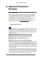
I. Introduction............................................................................................................................... 50
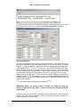
a) SpecProc Processor ............................................................................................................... 50
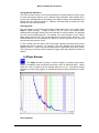
b) GSpec Browser ....................................................................................................................... 52
c) Reprocessing Spectral Data ................................................................................................... 53
7.
Glossary..................................................................................................................................... 55
a) Acquisition Panel..................................................................................................................... 55
b) Browser ................................................................................................................................... 55
c) Browser & Processors Panel .................................................................................................. 55
d) Client Process ......................................................................................................................... 56
e) Communication Panel ............................................................................................................. 56
f) Configure Communication Settings Box ................................................................................. 56
g) Configure Tool Settings Box ................................................................................................... 56
h) Dashboard............................................................................................................................... 57
i) Data Handler ........................................................................................................................... 57
j) Data Pipe ................................................................................................................................ 57
k) Depth Mode............................................................................................................................. 57
l) Depth Panel ............................................................................................................................ 58
m) Depth Reference ..................................................................................................................... 58
n) Encoder Pulses Per Turn........................................................................................................ 58
o) Encoder Type.......................................................................................................................... 58
p) Full Wave Form Tool............................................................................................................... 58
q) Header .................................................................................................................................... 59
r) Image Tool .............................................................................................................................. 59
s) LAS file .................................................................................................................................... 59
t) MSLog.ini File ......................................................................................................................... 59
u) Multi-channel Tool................................................................................................................... 59
v) Panels ..................................................................................................................................... 59
w) Processor ................................................................................................................................ 59
x) RD-File .................................................................................................................................... 60
y) Replay Mode ........................................................................................................................... 60
z) Record Mode........................................................................................................................... 60
aa) Sampling Mode ....................................................................................................................... 60
bb) Sampling Rate......................................................................................................................... 61
cc) Serial (RS232) Cable .............................................................................................................. 61
dd) Thread ..................................................................................................................................... 61
3
ee) Time Mode .............................................................................................................................. 61
ff) TOL file.................................................................................................................................... 61
gg) Tool Category.......................................................................................................................... 62
hh) Tool Panel ............................................................................................................................... 62
ii) Wheel Circumference ............................................................................................................. 62
jj) Well Log .................................................................................................................................. 62
kk) Logging cable.......................................................................................................................... 62
ll) Cable Head ............................................................................................................................. 63
mm)
Rehead ............................................................................................................................ 63
nn) Sonde ...................................................................................................................................... 63
oo) Mud Plug ................................................................................................................................. 63
pp) Slip Rings ................................................................................................................................ 63
qq) Winch ...................................................................................................................................... 63
rr) Measuring Head...................................................................................................................... 63
ss) Bulkhead ................................................................................................................................. 64
tt) Probe Top ............................................................................................................................... 64
uu) Armor....................................................................................................................................... 64
vv) Conductor................................................................................................................................ 64
ww) Mecca Connector .................................................................................................................... 64
xx) Mecca Pressure seal .............................................................................................................. 64
yy) Mecca Boot ............................................................................................................................. 64
zz) O-ring ...................................................................................................................................... 65
aaa)
Continuity ......................................................................................................................... 65
8.
Appendix ................................................................................................................................... 66
I. MSLog.ini file example ............................................................................................................. 66
II. Sample TOL file......................................................................................................................... 67
ai IMPORTANT WARNING!!!!! ................................................................................................... 67
III. Pulse Discriminator Settings for the MGX II .......................................................................... 72
a) Overview ................................................................................................................................. 72
b) Theory of Operation ................................................................................................................ 72
c) Tol files and Discriminator settings ......................................................................................... 72
ci Discriminator parameters explanation .................................................................................... 73
d) Manual Discriminator Settings ................................................................................................ 73
e) Procedure for determining Manual Discriminator Settings ..................................................... 74
ei Equipment needed.................................................................................................................. 74
f) Discriminator pulse testing for positive discriminator.............................................................. 74
IV. Depth Offset Control in Tol Files ............................................................................................ 78
a) Introduction ............................................................................................................................. 78
b) Tol file configuration ................................................................................................................ 78
4
MSLog for MGX II Operator Manual
1. System Overview
I. Introduction
The MGXII Logger acquisition system is based on modern electronics design in which
software control techniques have been used to the best advantage. The hardware
incorporates the latest electronic components with embedded systems controlled via the
specially developed MSLog Windows interface program.
The software takes advantage of the Microsoft Windows  family of operating systems.
These multi-tasking software platforms can accommodate all the tasks necessary for
maximum data security and ease of operation.
The system design philosophy is unique in two respects. First, it has been built to
accommodate several generations of single conductor, Mount Sopris tool types, and
second, it is totally software controlled.
The basic system design criteria are as follows:
•
Windows 95, 98, NT, 2000  operating systems platform
•
Rugged, fault tolerant electronics
•
Easy to use, on-screen graphical user interface -The Dashboard- with selfdiagnostic features, system configurable through screen dialog boxes, with
minimal technical knowledge needed by the user.
•
Wire line and winch flexibility - runs on most coax, single and multi-conductor wire
lines with compatible probes.
•
Depth encoder flexibility - compatible with most 12V or 5V AB quadrature and
pulse shaft encoders, and configurable for any combination of wheel/depth pulses
per revolution.
II. Setting up the System
a) Serial Cable
The standard, nine pin, serial cable is the interface between the PC and the MGX II
Logger.
b) Setup Connections
!
Insure that the power supply cable is connected to the MGX II. Insure that the serial
cable is connected to COM1. Connect your printer to the printer parallel port, LPT 1,
checking first that the printer is turned off. Even if you don’t have a printer connected to
the PC, MSLog log display functions will not work unless a default printer is set up
on the PC. If one is not installed (such as when starting out with a new PC, install at
least one printer.) Finally, connect the PC power cable to your external power supply.
The system is now prepared for operation. Read Chapter 3, System Operation before
you apply power to the system.
P/N 7000164G
5
MSLog for MGX II Operator Manual
c) Logger Configuration
The user should read and understand details of the MSLConfig program, which is
automatically started during MSLog software installation. The user should have
information about the logger, winch, and probes to be used so that the system and
software are properly configured. For details click on Help when running the MSLConfig
program, which is located in \MSLog\Utils
2. Software Architecture
I. Introduction
The acquisition system software runs on the Microsoft Windows 9X ™, Windows NT™,
or Windows 2000™ operating systems. The system software was developed using the
Microsoft Win32™ applications programming interface (API), which allows applications to
exploit the power of 32-bits on all Microsoft Windows ™ family of operating systems. The
Microsoft Win 32 API can support more than one process (executable programme)
concurrently. Moreover a process can consist of more than one thread, i.e. operational
task, where threads are the basic entity to which the operating system allocates
processor (CPU) time.
The MSLog software exploits the true pre-emptive multitasking ability of the Win 32
environment. Within the system threads are allocated a priority rating. The priority rating
is designed to optimise the data security features of the system while maintaining an
environment that is exceptionally responsive to the user. The multitasking environment
also means that you can have more than one application running at once.
P/N 7000164G
6
MSLog for MGX II Operator Manual
II. The Dashboard System
a) Overview
In the MSLog program the graphical screen interface used by the operator is called the
Dashboard. The Dashboard system consists of multiple threads, running concurrently,
that handle specific system tasks. The system currently controls the six functions listed
below:
1.
2.
3.
4.
5.
6.
Data Handler
Depth
Tool Power
Data Display
Configure Tool
Configure Communications
Top priority is given to the thread that controls the Data Handler task. There are three
tasks that are related to window panels that remain constantly available on the screen:
the Depth Panel, Tool Panel and the Data Panel. Two other threads are related to tasks
that interact with dialogue boxes, Configure Tool and Configure Communications. The
multi-thread architecture allows the system to run different tasks concurrently, e.g.
updating the depth counter at the same time as acquiring data from the tool. Items 2-6
are always available on the dashboard.
Information specific to a particular tool is contained in a unique tool configuration file
which will have the extension name *.TOL. Information contained in the *.TOL file is used
by different components of the system for initialising Dashboard components (tool power,
data protocol etc.), as well as setting parameters for Client processes, where a “Client”
process is an application handling data processing, data display or printing. Of the six
operational tasks top priority is always given to the Data Handler screen, either
maximised as an open window or as a minimised toolbar.
As mentioned above, tool information is kept in *.TOL files which normally reside in the
\MSLog\Tol\Current directory. Winch specific information is held in the MSLOG.INI file
in the \Windows or WinNT directory. The file contains information on parameters such as
the depth encoder characteristics and measure wheel dimensions, cable length and type.
P/N 7000164G
7
MSLog for MGX II Operator Manual
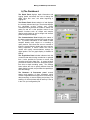
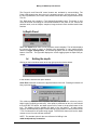
b) The Dashboard
The Depth Panel displays depth information and
logging speed, and allows the user to change the
depth value and “zero” tool when beginning a
logging run.
Tool Power Panel allows selection of and displays
the currently selected tool type. The window displays
the calculated up-hole voltage and current
consumption and provides the means to switch tool
power on and off. It also provides control of tool
specific functions such as Caliper and sampler
opening and closing as well as image and acoustic
probe configuration settings.
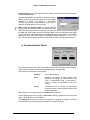
The Communication Panel displays the status of
the data communication between the logger and the
PC. It provides information on the number of data
samples already read, unique to a recording or
replay session, and counts the errors or number of
times the system failed to obtain data upon request,
during acquisition. A button allows the user to
access and modify communications settings for
digital probes. The bar graph display is disabled in
MSLog.
The Acquisition Panel window indicates both the
current file that data is being recorded to or replayed
from. It also provides the means to record, stop
recording and replay data files. A second window
provides the means to switch the acquisition system
from time to depth recording mode. The Settings
button allows the user to specify different time and
depth digitise intervals, and provides the capability to
save the settings
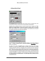
The Browsers & Processors panel controls
starting and stopping of client processes, which
consist of applications that support such functions as
data processing, on-screen display and printing. The
selection of client windows that will start up is set up
in the TOL (tool configuration) file.
P/N 7000164G
8
MSLog for MGX II Operator Manual
3. System Operation
I. Starting MSLog
Refer to Chapter 1 for details on how to connect the system
!
After verifying that all connections are correct, turn on the power to the PC, and allow
the operating system to finish completely loading. Turn on Power to the MGXII. You
should see the MGXII depth display flash “-8888.8”, and then display the last depth value
stored in the logger. The right side “TO PC” data light should blink. If the “TO PC” is not
blinking, turn the Logger power OFF then ON again.
If you are unfamiliar with Windows operating system then please refer to the Windows
user manual for guidance on the basics of the system's operating platform. It is assumed
that the user has basic knowledge of Windows.
MSLog
To start the MSLog program, left click on the Start button on the status bar, and holding
down the left mouse button, move to Programs>MSLog>MSLog. Release the button
and the system will automatically load the MSLog operating software and present you
with the control Dashboard at the left of the screen.
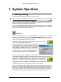
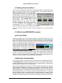
At start-up of the program, MSLog will attempt to communicate with the
MGX II. A small logger replica will appear:
If the MGX II, logger is not detected by the MSLog program, a warning
message appears. This message will appear if the MGX
II is not properly connected by serial cable, or if the serial
cable is bad, or if the MGX II power is not turned on and
correctly initialised. Note that the program can be run in
Demo Mode on any PC to replay previously logged data.
For more information, refer to the section on REPLAY.
When the MGX II logger is detected, MSLog sends
commands to configure the MGXII. The logger replica icon that mirrors the status LED’s
on the MGXII Depth display appears on the screen until the command
sequence is completed. During this time MSLog will not accept further
mouse clicks. The logger replica icon also appears at tool selection and
again when tool power is turned on. It is displayed to show the user that
the logger and PC are communicating with each other in a “SETUP” mode, The user
should not press any keys or click the mouse until the box disappears.
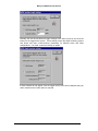
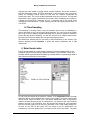
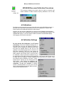
During the initialisation sequence, if the PC and logging system have been set up at the
factory, or the software has been previously installed and configured, the system will
normally start up and the DASHBOARD will appear on the left hand side of the screen. If
the PC has not been set up for the logger, and the initialisation settings in the MSLOG.INI
file are different than those set up in the logger, the following boxes may appear:
P/N 7000164G
9
MSLog for MGX II Operator Manual
Normally, the user should allow the logger settings to be used, since they are set at the
factory for the logger/winch system. These settings control the depth measuring system
and power and data communications parameters for different winch and cable
configurations. If in doubt, contact the factory for details.
If these windows do not appear, then the logger and PC have been initialised during an
earlier session and no further action is required.
P/N 7000164G
10
MSLog for MGX II Operator Manual
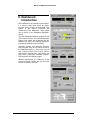
II. Dashboard
Introduction
The Dashboard is the operator’s control panel.
It is used to select and control all system
functions and to monitor acquired data. This
section of the manual introduces the
components of the dashboard. More details
can be found in the “Dashboard Operation”
section.
The main Dashboard window occupies the left
of the monitor screen. The standard Windows
screen icons remain active onscreen but are
shifted to the right of the MSLog Dashboard,
they can be accessed in the usual way.
Operators familiar with Microsoft Windows
may recognise some of the controls found on
the Dashboard while to others they may be
new. Features used include push buttons,
radio buttons, check buttons, check boxes, text
entry fields, graphically simulated switches,
LED indicators and LED bar graphs.
Whether experienced or a newcomer to the
concept of virtual controls, the user will soon
become confident in their use.
P/N 7000164G
11
MSLog for MGX II Operator Manual
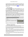
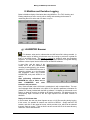
Right clicking with the mouse while over the Logger Dashboard opens the menu shown
below:
Options are:
Always on top Dashboard window always above other windows.
Autohide
Dashboard hidden when area outside is made active by pointer.
(Dragging the pointer to the extreme left of screen re-opens the
Dashboard).
Help Index... Click to enter the help document. It is fundamentally a copy of
this document with some enhancements.
About MSLog Program and hardware set up details.
Exit
Closes MSLog (which closes open data files, and powers down
MGXII if this has not already been done).
III. Dashboard Panels
The Dashboard window contains five sub windows or panels, all of which can be
maximised or minimised using the top right window control buttons common to Windows
applications. These windows cannot be permanently closed.
Depth
Tool
Communication
Acquisition
Browsers & Processors
depth settings
tool configuration & power
data flow & communications controls
data sampling & replay controls
data browsers & processor controls
When in an active state control buttons are sharply outlined. The user will notice that
some controls are either permanently or temporarily grey. This is an indication that the
function is not yet implemented or that operation of the control is not appropriate at the
current state of the system. For example Replay cannot be accessed when Data
Sampling is On.
A display light (or LED) at the top left of the each panel indicates
system status. The color green indicates a correctly functioning system, and a red color
indicates a fault. This is generally true of all panels on the dashboard. Throughout this
document, these display lights will be referred to as LEDs, which is an acronym for Light
Emitting Diode
P/N 7000164G
12
MSLog for MGX II Operator Manual
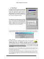
a) Tool Panel
The Tool panel is used to select the desired probe
for logging, switch tool power on and off, access
tool functions such as Caliper open/close, and to
modify tool configuration settings. Access to
secondary windows, is provided when required, for
setting additional tool parameters. Depending on
the probe being used, tool power may have to be
On to access Tool Settings/Commands.
The logging tool is selected from a pull down list
box which displays the tools available as described
by the *.TOL files loaded in the \MSLog\tol\current
directory. After the desired tool is selected with the
mouse or highlight bar, a window will pop up
asking the user to confirm the selection. An
example of such a window is shown below:
If the YES button is pushed, the MSLog software reads the information in the TOL file
associated with this selection, sets up the MGX II logger power supply and data protocol
system, and loads the relevant “browser” clients for log data display. During this time,
the logger icon will flash, indicating the system is busy. Also, the browser
clients will load, based on the configuration in the TOL file. Normally, for
standard logging tools, the MSIPROC, MCHNUM, MChCurve, and
LASWRITER Clients will start. For image and full wave sonic tools, other Clients will
start. The functions and features of these Clients are discussed later in this document. If
a browser fails to start within a reasonable time, a “not connected” message will
appear. The user should go to the Browser window, select and Close the browser, and
“Start” it again.
Two bar meters on the Tool Panel display the tool voltage and current supplied by the
MGXII logger to the probe. These values are calculated from information read in the TOL
file and winch/cable information.
The current meter is active but should show 0 mA until the tool power button is pushed.
These meters are not diagnostic, in that they only display the values read from the TOL
file. The voltage at the logger can be measured at the red and black banana jacks on the
logger, if desired.
P/N 7000164G
13
MSLog for MGX II Operator Manual
The Power-On and Power-Off control buttons are activated by mouse-clicking. The
Power LED shows green when the tool is powered correctly, and red when off. When
the tool is powered on, the current meter should indicate the value programmed from the
TOL file.
The Tool panel also contains a Tool Settings/Commands button. This button is only
active when there are settings or commands available for the probe in use. Controls for
particular tools, such as Calipers, samplers, image, and sonic tools are discussed in later
sections.
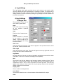
b) Depth Panel
Within the Depth Panel there are two separate numeric displays. The left side displays
the current tool depth in metric or English units (depending on user preference-see
details on Logger Configuration). For the MSLog system, this is normally the physical
bottom of the tool. The right side displays the current logging speed in depth units per
minute.
bi
Setting the depth
Clicking on the link window button at the top right opens the window below:
In this window, there are two option buttons:
Set to Zero-resets the counter to the physical bottom of the tool. Pressing this button will
bring up a new window:
This window prompts the user to position the probe top at the zero reference point to
begin logging (normally ground level). After probe is positioned at zero, the user should
then press the YES button, and depth system will be reset to the physical bottom of the
tool. The display will then indicate the depth of the tool bottom. All other sensor
positions are automatically depth corrected during logging based on values read from the
*.TOL file selected for the probe being logged. Note that this feature will set the depth
counter to zero if no tool has been selected.
NOTE: The standard point for the zero reference for MSLog is the
cable-head/probe top connection.
P/N 7000164G
14
MSLog for MGX II Operator Manual
Change Depth-opens depth change window, which is activated by entering new depth
and pressing OK button.
Note that depth data is processed as a separate task in
MSLog. In the event of a power failure, the current depth
information is stored in the MGX II in non-volatile
memory. If the probe is kept stationary, and power is
restored, the valid depth will be recovered.
!
When using an isolation bridle (for normal resistivity
logging), the user should position the bridle/cable head
connection at the zero reference, and then press the “Set to Zero” control, and then after
the depth has been update, press the “Change Depth” control and add the bridle length
(e.g. 25 feet) to this depth and enter it into the field to set the correct depth. For example,
using this method, the correct depth for a 2PEA/PGA probe would be 6.17 + 25 = 31.17
feet. The user should physically measure the bridle to insure accurate depth reference
c) Communications Panel
The communications panel shows information about the data sampling, data throughput,
and provides the facility to tune communications settings as appropriate.
There are three LED panels, which display:
Data/sec
rate of data sampling
Data
Indicates the number of data samples read
unique to a recording or in a replay session. The
value is automatically reset to zero when a
record or replay is terminated by the Stop
control
Errors
Counts the errors or number of times during
acquisition that the system failed to obtain valid
data upon request.
When data is not correctly received, the No Data LED shows red.
The bar graph meter at the top right is not active in MSLog operations, and is used only
with the ALTLog version of the software.
The Settings button options are further discussed in the Logging Procedures, and relate
to the adjustment of communications parameters in the MGX II logger.
P/N 7000164G
15
MSLog for MGX II Operator Manual
d) Acquisition Panel
The Acquisition panel is used to select data recording mode, set sampling rates, start
and stop data recording, edit information in the log header, and replay data.
Sampling mode is selected through the combo pull down list box. Options are Time,
Depth Up, and Depth Down. In depth mode sampling is directly related to the pulse
inputs from the depth encoder device and the settings in the MSLog.ini file. The Settings
button opens a dialogue box in which the sampling or time interval can be set by the
user. Edit the values as required and confirm with OK.
To start sampling select the On button. The LED changes to green when sampling is
active.
DO NOT CHANGE DEPTH SAMPLING INTERVAL while logging, without
starting a new data file.
To record a file to disk, the Record button is selected. This opens a file manager
dialogue box in which the operator chooses the location and file name for the data
recorded. Recording commences immediately after the filename has been entered and
confirmed by Save. The file name is displayed in the text box at the top of the acquisition
panel. MSLog automatically adds the file extension .RD to all data files, and this binary
file format can be viewed/plotted again using the Replay button. If LASWRITER browser
is active during logging, an LAS format data file is also created, which follows the LAS
(Log ASCII Standard) v 2.0 standard. This file format can be imported into most log data
processing or Windows compatible data base manipulation programs. Depth corrections
are not preserved in LAS format files. For more details, see the section on the
LASWRITER browser.
P/N 7000164G
16
MSLog for MGX II Operator Manual
By pressing the Header button, the user can edit and save header information. More
details are found in the Logging Procedures section. Custom headers can be created
using the HeadCAD program (a WellCAD module). They should be copied to the
\MSLog\Headers directory, and given the name default.wch. Currently, the header file
cannot be larger than 64 Kb. This means that custom bitmaps may need to be reduced
in size/resolution to fit into this limit. Otherwise the bitmap may not print or view.
To replay data (from the .RD file), first check that sampling is turned Off. The Replay
button then becomes active. Clicking on the Replay button opens a file manager
dialogue box in which the operator may choose the file to be replayed. Note that before a
file can be replayed the correct image browsers and processors must be open. All
browser functions can be accessed before replaying the data, including printer on/off,
curve and log scaling, etc. To stop the replay at any point, click on stop. The original
header recorded in the log cannot be changed, as it is a permanent part of the RD file.
If, for some reason, an LAS file was not generated during the original logging operation, a
new LAS file can be created during REPLAY. See details under the LASWRITER
browser section.
Sampling settings remain in place if the tool power is switched off provided that the tool is
not deselected.
e) Browsers & Processors
The Browsers and Processors panel contains a combo list box, which shows the image
and data processing drivers available for the tool selected. A browser is a data-viewing
window. A processor manipulates the data for presentation of a particular type of log.
Most tool calibrations Caliper, EM, etc., are made using the MCHNum browser. MSIProc
is used when more than a linear calibration needs to be applied to data so it is not always
used. The MSIPRoc processor must be running if it is included in the Browser list.
Typical MSI tool options are shown above. Some of these drivers will be activated and
open on screen when the tool is selected but any may be started or closed by
highlighting the selection and clicking on the relevant control buttons. This facility can be
useful when modifying a *.TOL file, e.g. display parameters. The parameters can be
changed in a text editor e.g. Notepad, and saved to file without powering off the tool. The
browser can then be closed and restarted with new parameters taking effect. Note that
each TOL file contains instructions on which browsers/processors are to be used for a
given probe. See the appendix for a sample TOL file description.
P/N 7000164G
17
MSLog for MGX II Operator Manual
IV. Logging Procedures
The general procedures for logging a tool using MSLog follow. Consult the tool operators
manual or the MGX II Tool Instructions.pdf for specific operating instructions covering
most tools.
• Configure the system for the tool to be logged.
• Connect the tool.
• Power up the tool.
• Verify communications.
• Verify tool operation.
• Calibrate tool if necessary ( MCHNUM Processor).
• Move tool to starting point and zero the depth.
• Set sampling parameters, and turn ON.
• Enter Header data.
• Run test log/adjust tool configuration.
• Modify image browser parameters as necessary.
• Record log.
• Process & print.
This assumes that *.TOL files with calibration factors, shifts etc., have been prepared for
the tools to be run.
a) Loading a Tool Configuration File
Select the tool file from the list of available tools shown in the Tool Panel combo list box.
The listed tool names are derived from the *.TOL files present in the \tol\current directory,
the name being that given as the [ToolName] parameter in the file. The user may edit the
[ToolName] if so desired, so that a customized name will show up in the tool name list.
The default location of the active *.TOL files is set in the MSLog.ini file and are setup
using the MSLConfig program.
In general, only the .TOL files that correspond to the system and set of downhole probes
being operated should be stored in the MSLog\tol\current directory. Depending on the
version of MSLog software installed, other .TOL files may be supplied, but will be stored
in the main \tol\ directory. These files may be installed at a later time, if required, using
the MSLConfig.exe program. Details of the MSLConfig program are found later in this
manual. Only install TOL files using MSLConfig, as simply copying the files may not
update required information regarding tool power requirements and discriminator
settings.
b) Data Viewers for Client Applications
Once a tool file has been loaded the system may, depending on the .TOL settings,
automatically open the relevant data viewers specific to the tool. Any processors relevant
to the tool will also be started. Both image browsers and processors are defined in the
tool *.TOL file.
P/N 7000164G
18
MSLog for MGX II Operator Manual
There are several different types of viewers and processors, all residing in their own
individual windows. The windows will appear on the screen unless set to load minimised.
They can all be re-sized or moved by dragging the window edges or corners, and can be
maximised, or minimised to a marker on the status bar. The default position and size of
each window is defined in the .TOL file and can be edited as desired.
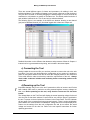
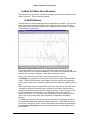
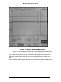
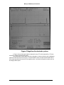
The following figure is an example of the MChCurve browser showing a raw channel
(cps) and a calibrated channel (cm) from data logged with a three-arm Caliper tool.
Detailed information on the different data browsers and processors follows in Chapter 4.
Instructions for log presentation and printing, are included in the same chapter.
c) Connecting the Tool
Having loaded the correct tool file you can then proceed to connect the tool to the wire
line cable. If you are in any doubt about the configuration of your system it is prudent to
power on the system without a tool and to check the voltages present on the conductors
of the cable head to make sure that they match the requirements of the tool. Always
check cable conductor isolation and continuity before connecting probes to the
cable head.
d) Powering up the Tool
!
Irreparable damage may occur to the tool if powered on while an incorrect tool file has
been loaded. Older tools in particular are less protected against incorrect voltages so
take care. Before powering on the tool, verify that the correct tool file has been
loaded.
The Voltage Meter on the Tool Panel will display the normal operating voltage for the tool
once the tool file has been selected. Current will be zero until the power is switched to
the tool. To power on the tool select the On button in the Power Panel. The LED indicator
will turn green if the command has been executed correctly. There is a short initialisation
period before tool communication is established. Voltage and current levels displayed on
screen are the settings from the tool configuration file and do not reflect the actual
voltage and current on the wire line. Refer to the tool specific instructions for further
operating procedures.
P/N 7000164G
19
MSLog for MGX II Operator Manual
di Powering and Operating Calipers and Fluid
Samplers
2CAA/2PCA Caliper Family-Caliper tools require special procedures to open and close
the Caliper arms. Generally, there are two different procedures for opening Calipers with
the MGX II system operating under MSLog. The procedure is specified by information
loaded by the .TOL file. Mount Sopris Calipers operate and open using negative voltage.
Pressing Power ON will cause a message such as the one that follows to appear for the
latest 2CAA/2PCA family of Calipers.
Normally, if the Caliper is at the bottom of the hole, or the user wishes to calibrate the
Caliper, the correct response is YES. However, for Calipers that operate in this mode
(such as the MSI Calipers), the user should not turn power on until the Caliper is at the
bottom of the hole. The normal logging sequence would be to calibrate the tool on the
surface, close the arms, and then zero the tool and proceed to the bottom of the hole.
The Depth System will display the correct depth even though tool power for MSI Calipers
should be OFF while going in the hole. When the Caliper probe is on the bottom of the
hole, the Power ON button is pressed, bringing up the window shown above. After
pressing YES, the Caliper will begin to open. Press the Tool Settings button, and press
OPEN, which will start the software timer. After 90 seconds has elapsed, a ”Caliper
Open” message will appear. To see if the Caliper is open on the bottom of the hole, the
user can go to the Acquisition Panel, select Time Mode, and turn sampling ON. A
reasonable value for the Caliper should appear in the MCHNUM data browser. Keep in
mind that often the Caliper arms do not fully open until the probe is raised a few feet
(meters) off the bottom of the hole. To close the Caliper after logging, the Tool Settings
Button is pressed to bring up the Caliper Operation Button, and the Close Button is
pressed.
For older Calipers, such as the CLP/CTP family, which operate on a lower voltage than
the new Calipers, the Tool Power ON button must be pressed to allow the Tool Settings
Button to be active. After pressing this button,
the Tool OPEN/CLOSE Button will appear.
Upon pressing either button, an Elapsed Time
display will appear during the OPEN or CLOSE
process. The user must wait until the DONE box
is activated, at which time the system is returned
to the logging mode.
Other Calipers not
manufactured
by
Mount
Sopris
(MLS,
Comprobe, etc.) will generally operate in this
mode. Fluid Samplers operate much the same
as Calipers, and the user will normally turn Tool Power ON, and then use the Tool
Settings Button to access the OPEN and CLOSE buttons for the sampler.
dii Image and Full Wave Sonic Tools
Probes such as the FAC40 and OBI40 imaging tools and full wave sonic tools, which
have many user configurable features, are also controlled through the Tool
Settings/Command Button. Detailed discussions of the settings are presented in the
Operations Manuals and browser sections for the individual probes.
P/N 7000164G
20
MSLog for MGX II Operator Manual
e) Verifying Communications
Verify correct communication between tool and surface system. A green light should
appear in the upper left corner of the Communication Panel. This light should stay green
when the Acquisition Panel is set to Time Mode
and Sampling is turned ON. For standard probes
(all MSI probes, except the high baud rate digital
probes like 2SAA and Image probes from ALT) no
further action is needed. The Valid Light should
also be green.
The Settings Button of the
Communication Panel is only active when
adjusting settings for high baud rate probes.
Communication settings and options vary from tool
to tool. Individual tool configuration and
communications set up is described in the
individual Operations Manuals for the high data rate probes.
Note that sampling should be turned off before adjusting tool or Communications
settings.
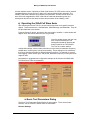
f) Calibrate tool (MCHNUM Processor)
g) Zero the Depth
The MSLog program uses the connection between the cable head and the top of the
probe as the zero reference. All log data is referenced to this point. Before lowering the
probe in the borehole, the probe zero point should be moved to the zero depth starting
point (or zero depth). After this has been done, click on the Depth Panel upper right hand
corner, to reveal the next window, which has two
buttons: The top button is used to set the logging
system depth to the tool bottom. This is based
on values that are found in the .TOL file for the
selected probe.
The software automatically
depth corrects the individual sensor offsets referenced to the tool bottom, with no user
action required. The tool length and sensor offsets in the *.TOL file are always specified
in metric units, whether operating in meters or feet. These settings are also used by the
browsers to depth correct the data which is displayed on screen or sent to the printer.
The user can edit this number by the appropriate amount (using “Change Depth”), if an
offset for the zero is required due to well-head access restrictions.
h) Setting the Sampling Rate
Prior to logging it will be necessary to set the tool sample rate. The sampling rate is set in
the Acquisition Panel, using the settings button for either time mode, or depth mode up/down, depending on the nature of the tool and your logging operation. Sampling rates
may be altered during the course of recording a log.
Note that the sampling rate may need to be reset if a different tool is selected. Sampling
rates can be set by default in the *.TOL file. Once again, the MSLOG system uses the
metric system as a basis for all measurement references. This means that measure
wheel circumference in the MSLog.ini file, tool and sensor lengths in the .TOL files, and
default sample intervals in the .TOL files should be entered in metric units. The system
then automatically converts to English units for the depth display, the sample interval
display, and the browsers. In general this will be transparent to the user, unless the user
operates in the English system of units, and finds it necessary to edit the INI or TOL files.
P/N 7000164G
21
MSLog for MGX II Operator Manual
Sampling rates are related to logging speed, encoder resolution, tool sensor resolution,
and data transmission rates. Since the depth data is derived directly from the encoder
pulses, the sampling interval cannot be less than the distance represented by
consecutive pulses. The volume of data transmitted varies from tool to tool. For high data
transmission rates, logging speed should be reduced. When considering tool resolution,
a density tool might have a resolution of 5cm. A sampling rate of 2cm would cause
overlapping of the data points. Typical sampling rates for non-imaging probes are 5 cm
or 0.10 feet.
hi Time Sampling
Time sampling is normally used to verify tool operation and to carry out calibrations. It
can be used when a tool is to be logged while stationary. For a tool such as the FAC40
with a high volume of data throughput a sampling rate of 500ms or greater is advised to
prevent the data buffer overflowing. You will also notice that on multiple channel tools,
cps values are much more stable with a longer time sampling interval.
The default time sampling rate for most tools is 1000 milliseconds (or one second). The
shortest sampling interval allowable is probe and system dependent and is 130
milliseconds.
i) Enter Header data
Prior to recording data, fill out the header information. Press the Header button on the
Acquisition panel. Once Recording is started the Header is not accessible. There are a
few basic header types distributed with MSLog. Note that MchCurve printed page width is
bound by the horizontal size of the header.
To edit a new field header push the button “Header” of the Acquisition Panel. A Header
editing box will be opened together with a layout of the Header. The layout of the Header
and all pre-set values are taken from a file named “default.wch” which is expected to
reside in the same directory as the file “default.wchc”. By clicking on the “value” field the
operator can type in his information. Also, the operator can directly fill in all information
from the previous logging run by clicking on the button “Last” of the Header editing box.
As soon as you click on the button “OK” the values in the file “default.wchc” are
overwritten or a new file “default.wchc” is created if no file of this name exists. The name
P/N 7000164G
22
MSLog for MGX II Operator Manual
of the directory where the file “default.wch” and “default.wchc” are expected can be
changed in the Tol file. Note: The header cannot be edited in Replay mode. For custom
header creation, consult Mount Sopris for more details. The HeadCAD program is
available for creating custom headers, which cannot be larger than 64 Kb. HeadCAD is
provided with WellCAD, or may be downloaded from www.alt.lu as part of the WellCAD
evaluation software.
j) Recording Data
Recording data to disk is not automatic, and MUST BE STARTED by the user. To do
this, click on RECORD in the Acquisition Panel. The system will then ask you to specify
a name and location for the file. Since this is a standard Windows file selection dialog
box, the user can also specify a new file folder in which to store the new data file. The
file will automatically be given a .RD extension (Raw Data). The .RD file can be
replayed with the MSLog system to provide additional copies of the log data, and can be
copied to disk and replayed on an office machine. The REPLAY button is used for this
function. The RD file is always created when Record is ON.
The RD file format is supported by the powerful WellCAD data processing software.
WellCAD can import depth corrected RD files for all MSLog generated data quickly and
easily, preserving all browser settings. Sonic data files must be processed by
SONPROC before import. To import RD files into WellCAD, simply select FILE,
IMPORT, SINGLE FILE, and chose RD as the type, and then navigate to the directory
containing the data file. See WellCAD documentation for more details.
If the user wishes to create an LAS (Log ASCII Standard) format, version 2, file that can
be imported into other data processing/presentation programs, this is done with the
LASWRITER browser. The LAS format produces data that is not depth corrected, and
the user should consult the Adobe PDF file describing each tool in detail for depth offset
information.
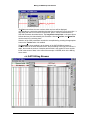
This LASWRITER browser must be running during
the logging operation if an LAS format file is needed.
The user should click on this browser to verify that
data is being recorded, and should see a window like
this:
The LAS file is automatically turned on and off by the
RECORD button, if the browser has been started.
k) Maximum Logging Speed
The maximum logging speed that the complete system can handle, given a particular
type of tool, will be controlled by one of the three situations discussed below.
If the surface system requests data at a rate faster than the tool is configured to deliver,
then there may either be errors in data received at the surface (tool specific), or the tool
may not respond at all. In this case the tool Communications Status window gives the
message ” no resp” i.e., no response.
Solution:
If this situation occurs it will be necessary either to re configure the tool
to send data faster (i.e. in the case of a televiewer, increase the speed of rotation of the
televiewer head) or reduce the rate at which data is being requested from the tool by
reducing the sampling rate - (Depth/Change depth sampling). The latter can also be
achieved by reducing the logging speed.
If the surface system requests more data than the tool can transmit through the wire line
for the given baud rate then the tool Communications Status window will give the
“overrun” message.
P/N 7000164G
23
MSLog for MGX II Operator Manual
Solution:
If this situation occurs it may be possible to diminish the amount of data
requested for each sample point by changing settings in the tool configuration. See
sections on image and sonic logging for details.
If the surface system requests and receives more data than the system can process in
real time, data may be lost. The system manages temporary data saturation through the
use of a data buffer. The buffer is a fixed size of emergency memory, which temporarily
stores data while waiting for the CPU to catch up.
!
Solution:
To lower the demand on the surface system and thus avoid data
saturation you can reduce the data transmission rate by logging more slowly or by using
a bigger depth increment for data sampling. In some instances with some tools (e.g. the
televiewer), the load on the CPU may be cut by reducing the number of dashboard
control windows open, (minimise them), and/or by reducing the number of client data
viewer windows open (similarly by minimising or closing down the windows.
l) Changing a Tool
!
Before handling or disconnecting the last tool used first ensure that tool power has been
turned OFF. Disconnect the tool. In the Tool panel select the new tool name to
reconfigure the system. Note that you may have to reconfigure the communications, tool
settings and sampling rates if the default values held in the tool *.TOL file have changed.
m) Replaying Data
To replay data from the Acquisition panel, it is a good idea to first go to the Sampling
Mode control and select Depth Up or Depth Down. This will make it easier to change the
depth scale when replaying data to a printer.
Then press the Replay button. The system will
prompt you for a file name with the extension
*.RD by displaying the file Open dialogue box.
After selecting the file for replay, confirm OK.
The browsers used during recording will then
connect. This may take a few seconds. The
system will then ask if you want to make any
changes to your current browsers (such as depth scale, filters, scales, etc.) and allow
you to enable printing and header style. The header cannot be edited in replay. After
these final selections are made, the OK button is pressed, and Playback will begin. Logs
recorded in Time Sampling Mode cannot be replayed, although the data can be read
from the LAS files and imported into other programs for further processing. It is possible
to create a new LAS file during replay by opening the LAS browser, and left clicking on
the task bar icon, and clicking on the Save on Replay line
mi Tool selection and replaying data
Rd data files contain an imbedded copy of the tool driver (.tol) file. Rd data files may be
replayed during log acquisition mode or Demo mode. In the normal log acquisition mode
if you replay a RD data file recorded with the currently selected tool driver type, then the
selected tool driver, not the embedded tool driver controls the settings for the replay. This
means that the currently selected tool driver settings for header, calibrations, browsers
running etc. are used to replay the data in the Rd data file.
This has serious implications if the calibrations of the imbedded tol file and the currently
selected tol file are not the same.
This behaviour can also be used to correct a log that was run with improper calibrations.
Re-calibrate the tol file and replay the RD data file after selecting the newly calibrated
tool driver.
P/N 7000164G
24
MSLog for MGX II Operator Manual
In Replay mode, if you do not select a tool from the list or select a tool of a different type,
the replay uses the settings from the imbedded tol file.
If you did not enter any header information in the original data, in replay mode you can
select the same tool driver, which will allow you to enter the header information. Just be
sure the calibration information, if any, is the same.
Although you cannot recreate the .rd file, you can fix data recorded with a browser turned
off by selecting the same tool and rewriting the .LAS file using that option on the
LASWriter, browser as described above. If a needed browser is missing from a tool
driver, data can be replayed with a corrected tool driver selected. You can use external
tol files, with corrected conditions such as calibration changes, to import data into
Wellcad.
The exact condition test for this replay behaviour is:
On replay MSLog uses the currently selected tol file on condition that ToolName=
matches (case insensitive) the imbedded one and DriverName= exactly matches
the imbedded one. Otherwise the imbedded tol file values are used.
n) Exiting MSLog
To exit, the user will turn TOOL POWER OFF, and then close MSLog. Right Click over
the dashboard, and select EXIT. The system will ask for verification and the user clicks
on YES to complete the shutdown of MSLog. As with all processes where the PC is
communicating with the logger, the user should watch the data lights on the logger
and verify that communications are complete. The logger will return to the power-on
mode (where the “TO PC” light is blinking at a steady interval.). DO NOT POWER OFF
the logger until this occurs.
P/N 7000164G
25
MSLog for MGX II Operator Manual
4. Browsers and Processors
I. Introduction
Once a tool file has been loaded the system will provide access to the relevant Data
Browsers and Processors specific to the tool type. The acquired data is provided in real
time to the individual clients (Browsers and Processors) window. By setting options within
the clients the user can control the layout for both onscreen data display and for hardcopy printout produced as a borehole document on site, calibrate probes such as
Calipers and other pulse type tools, record LAS format files, and edit and print
customized API style log headers. Specific formats can be saved so that they can be
called up again on the next logging job.
II. Multi Channel Client Data Windows
This family of display windows is a general-purpose suite that is used for logs where
each trace is composed from a single data value at the sampling point.
NOTE: After performing calibrations with MCHNUM, be sure to Close and re-Start
all browsers and processors. If you do not do this, calibration information will not
be available to the browsers and processors, which can result in erroneous data in
plots and the .las file.
P/N 7000164G
26
MSLog for MGX II Operator Manual
a) The MChCurve Browser
This browser has three pull down sub menus File, Edit and View
ai
File
This menu contains the options Print, Print Setup, Page Setup, and Exit.
Print This selection instructs the system to send the file
data to your printer.
Print Setup The default choice is Windows printing. Do not
select real time Printrex printing. You should select your
default Windows printer, which will provide for correct
scaling and resolution. Do not change this default setting,
unless you have changed your default Windows printer, or
the printed depth scales may not correspond to the
selection made by the user.).
The user can select whether a full header or short headers will be
Page Setup
printed). Short headers contain only curve name and scale information.
Exit This selection always returns user to previous menu.
aii
Edit
This menu contains options Depth Scale, Depth
Settings, Depth Column Position and Log Settings.
Depth Scale User selects the desired depth scale.
P/N 7000164G
27
MSLog for MGX II Operator Manual
Depth settings Allows user to specify horizontal grid settings for depth lines on log plot.
Depth Column Position User selects the position of the depth track (API standard is
30%=40%). User can change as required.
Log settings Accesses the Well-Log Settings dialogue box via the Select a Log list box.
This box is more easily accessed by clicking on the log name in the header. Changes in
log settings are automatically written to the \tol\current\ version of the TOL file so they are
available the next time the tool is selected.
aiiiView
Tool Bar contains buttons to turn on Printer, change Depth Settings, and view Browser
version number.
Status Bar shown below displays data related to Current Depth, Numbers of Data
samples, Numbers of errors, and the connection status. This is useful when Auto hide is
selected for the main Logger panels.
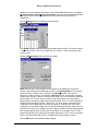
b) Depth Settings Dialogue Box
The depth settings dialogue box shown at right
is used to set the depth scale and grid layout
displayed in the MChCurve window.
Depth
Scale - set the depth scale of the log e.g. a
number 50 equals 1:50 scale, or 1 cm on
screen or printer will display or print 50 cm of
log. This is the scale that will be displayed
and/or printed.
Horizontal Grid Spacing - sets the frequency
of major and minor grid lines and
corresponding depth value text display. For
example, a value of 10 will produce a depth
number each 10 feet or meters, a bold grid line at each 5 and 10 unit spacing, and a light
grid line each unit. The user should not enter a value that results in a minor grid line
being printed at a frequency higher than the depth sample interval. For this example the
sample interval should be less than 1 depth unit. If in doubt, always start with a large
number like 100 for depth scale, and 10 for grid spacing. Problems can occur when
combining low value depth scales with low value horizontal grid spacing, when the minor
grid lines are forced to try to display or print at a higher resolution than the data sampling.
P/N 7000164G
28
MSLog for MGX II Operator Manual
c) Log Settings
The Log Settings menu option provides the user with access to the controls, which
govern the display and print characteristics for individual log traces. The easiest way to
reach the menu is to click on the log name in the header above the log display. The
settings selection can also be made by clicking on log settings in the EDIT selection on
the main menu task bar.
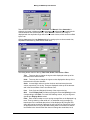
d) Log Settings
Dialogue Box
The parameters, which can be
set for each log trace follow:
Name
Enter a title of your choice using
all the standard keyboard
characters.
Units
Enter the units of measurement
Position
Enter the location in % full scale
for the location of the curve
relative to the full width of the
log plot. Well Logs can occupy
the same location.
Scale - Low
Select the minimum scale value. This value will appear on the top left hand corner of the
log Title bar, if there is sufficient room.
Scale - High
Select the maximum scale value. This value will appear on the top right hand corner of
the log Title bar, if there is sufficient room.
Logarithmic
By clicking this box, the user can select a logarithmic grid display, and enter the number
of decades. If the box is unchecked, the display is linear (default).
Grid
The values in the Grid box determine the frequency between vertical grid lines. Thus a
value of 10 in the Grid box means that a vertical grid line will be drawn every 10
measurement units. A value of zero will produce no vertical grid lines. This field only
applies when scaling is in linear mode. Use only one grid per section of plot area when
plotting multiple curves in that area.
Display Grids
Turn on or off the vertical grid lines.
Curve Styles
This selection allows the user to choose between solid and dash/dot line styles.
Color
P/N 7000164G
29
MSLog for MGX II Operator Manual
Allows selection of the color of the log curve from the available color palette. Choose
dark colors for monochrome printing, as light colors will not print on monochrome or grey
scale printers. While MSLog will display all colors on screen, it will only print in
monochrome in the present version of software.
Pen Width Controls the thickness of the log trace from 0.1mm up to 1.0mm.
Filter Width
The filter width function enables you to filter your log data on a moving average basis.
Thus by selecting a filter width of 5, a calculated moving average log, based upon five
incremental data points, will be displayed. By using the filter, spiky data can be
smoothed. Data gaps in well logs can be overcome by using an appropriate filter so long
as the data missing does not exceed more than 9 incremental units. Note that the filter
does not change the actual data, but is applied "on the fly" while the data is displayed
only. This leaves the data untouched and allows you to later reduce your filter width if you
wish to do so.
OK
Puts into operation your selected log parameters and returns you to the Multi-Channel
Curve Window, and saves the current settings in the \tol\current version of the TOL file.
Cancel
Cancels your selection and returns you to the Multi-Channel Curve Window.
P/N 7000164G
30
MSLog for MGX II Operator Manual
MCHNUM Processor/Calibration Procedures
This processor displays the numeric value for each tool channel, and
allows calibration of data channels requiring calibration, such as EM,
Caliper, etc..
di Calibrations
By clicking on the green ball icon on the upper left corner of the MCHNUM processor, a
pull down menu is provided, that allows the user to turn calibrations on and off, and
further access to the calibration settings for each channel.
Normally, the user will leave calibrations on (with the Use Calibration selected) when
logging. This results in the calibrations being applied to the MCHNUM, MCHCURVE, and
LASWRITER outputs. If the user wishes to watch raw data in the MCHNUM display
while logging, the can be unchecked.
dii Calibration Settings
Be sure that the Use Calibration is OFF before
proceeding! Click on the Calibration Settings line. In
this dialog box, the user can select the channel to
calibrate, enter the appropriate calibration values, and
then store the entered values in the TOL file The
example on the following page shows a screen for an
EM probe calibration, where the user placed the
probe in a zero conductivity medium and pressed the
button marked “Use Current Value” to set one end of
the calibration, and then placed the calibration ring on
the probe with a 458 mS/m response and pressed the “Use Current Value” button to set
the other end of the calibration. Similar calibrations can be performed for Calipers, using
two different known calibration ring sizes. When
finished with a channel, the user should press the
Store button. After finishing the calibration, the
user should close the window, and CLICK on Use
Calibration, so the is checked. If another
browser, like MCHCURVE, is running, the user will
have to Stop and Start the browser again to make it
read the new calibrated values.
P/N 7000164G
31
MSLog for MGX II Operator Manual
diii Sample Calibration Screen
Caution: The user must follow the above procedures to the letter to ensure
accurate and correct calibrations. Pay close attention to the reference to the
check mark () setting in front of USE Calibrations. It is OFF during calibration
and ON during logging.
e) MsiProc Data Processor
The MSIPROC Processor provides data format conversion, and must be running for
those probes requiring this function. This processor will automatically start when
initialised by the Tool selection dialogue. The user should make sure that it is running
during calibration and logging. Do not turn off MSIPROC, or incorrect data will be
recorded. If it is listed in the Dashboard Panel as a processor, it must be running. Many
probes, such as stand-alone gamma, image, and sonic do not require MSIPROC.
After performing calibrations with MCHNUM, be sure to Close and re-Start
MSIPROC and other browsers.
P/N 7000164G
32
MSLog for MGX II Operator Manual
f) MchProc Data Processor
The MchProc Processor is an updated version of MSIProc and will eventually replace it.
It operates just like MSIProc and all comments on the operation of MSIProc apply to
MchProc. Both processors are used to retain compatibility with existing and custom tol
files. MchProc has additional functionality similar to Wellcad for math and logical
functions including special Deviation logging algorithms.
fi MchProc and Deviation Logging
Deviation tool files enable access to dialogs allowing the setting of measuring Units and
Declination offset. To do this, right click the top of MchProc as shown in the following
graphic.
Clicking Unit opens the following dialog:
Select the units you wish to use for the deviation TVD, Northing, Easting calculations.
Clicking Declination opens the following dialog:
Enter the declination offset for your location.
P/N 7000164G
33
MSLog for MGX II Operator Manual
fii MchNum and Deviation Logging
Below is MchNum display of deviation data using MCHProc. The TVD, Northing, and
Easting endpoints are set to zero by either closing and restarting the browsers or
reselecting the tol file at the end of a down or up run.
g) LASWRITER Browser
This browser, when active, indicates that an LAS format file is being recorded. In
the present version of MSLog, this browser must be running to produce a log data file
that is in an ASCII format. This format is required for import by other log processing
programs. The .RD file recorded by MSLog is only used for REPLAY of logs with MSLog
software or direct import into the latest version of WellCAD software.
A green light, and the name of the
current file in the box, indicates that
recording is taking place in the location
specified. If the LASWRITER browser is
closed by accident, go to the Browsers
and Processors Panel, and re-select
LASWRITER, and press OPEN to restart it.
After performing calibrations with
MCHNUM, be sure to Close and reStart
LASWRITER
and
other
browsers and processors.
Note: Data recorded in the LAS format is recorded as is, with no depth offsets. The user
can find depth offset information in the MGX II Tool specific operations information file
(Adobe PDF format) included with the MSLog software. All depths are referenced to tool
bottom, so data will need to be shifted up for depth corrections. RD playback logs are
automatically depth corrected as are RD logs imported into the latest versions of
WellCAD.
Replay of LAS format data
In some cases, the user may have forgotten to turn on LAS file recording during logging.
If this occurs, it is possible to create a new LAS file in REPLAY. Simply start the LAS
browser, and click on the upper left corner, which provides a line, which can be selected
that says “Save on replay”. Click on this line to save a new LAS file in the same directory
where the *.RD file was selected.
P/N 7000164G
34
MSLog for MGX II Operator Manual
5. Image/Full Wave Sonic
Tools
I. Introduction
Several types of specialty tools can be operated with the MGX II logger and MSLog software.
The basic operation of these tools is covered in this section. For additional details, the user
should consult the individual documentation for each probe.
II. Mount Sopris Instruments Sonic Probes
Mount Sopris currently has three, versions of Full Waveform Sonic Probe the 2SAA-1000 the
2SAA(F)-1000 and an anticipated 2SAF-1000. The 2SAA-1000 is a one transmitter multiplereceiver probe while the 2SAA(F)-1000 or 2SAF-1000 can accommodate either a second,
2STA-1000, transmitter, or the 2SNA-1000 probe section, added at the top of the probe. The
2SNA-1000 provides a natural gamma radiation measurement to the Sonic measurements.
The transmitter from a 2SAA-1000 can be upgraded, at the factory, to operate as a 2SAA(F)
by replacing its microprocessor firmware. The serial number of the 2STA-1000, transmitter
section will have an “F” stamped on it to indicate that it has the 2SAA(F)-1000 firmware.
In MSLog both the 2SAA(F)-1000 and 2SAF-1000 use 2SAF-1000 browsers/processors. The
tol file descriptions are different because we anticipate the tool length will be different. The
model number of the Sonic Tool will change to 2SAF-1000 when the new transmitter design is
finished.
a) ALT FWS Sonic Probes
Mount Sopris Instruments has offered the ALT FWS 40 full wave sonic probe. Additionally the
ALT FWS electronics have been used to upgrade older, analog or digital sonic probes so they
are compatible with MSLog or the Altlogger
III. Mount Sopris 2SAA/2SAF Full Wave Sonic
Probe
The Mount Sopris 2SAA-1000 full wave sonic probe can be configured in a variety of
transmitter/receiver combinations. Each combination requires a specific TOL file, which
describes the probe layout. The most basic (and most common) configuration is a single
transmitter/two receiver probe, with the transmitter located on the bottom of the probe. The
receivers are then located 3 feet and 4 feet above the transmitter.
Mount Sopris supplies TOL files for each probe, as required, and the user should contact the
factory for additional files as needed.
Additionally there is an upgraded version of the 2SAA-1000 designated the 2SAA(F)-1000. It
has the capability to operate with one bottom transmitter or two transmitters, one above the
top receiver and the other below the bottom receiver each separated from the receivers by an
P/N 7000164G
35
MSLog for MGX II Operator Manual
acoustic isolation section. Optionally a 2SNA-1000 Gamma, SP, SPR section can be inserted
immediately above the top receiver in place of the top transmitter/isolator assembly. The
2SAA(F)-1000 uses a different set of browsers and processor. A newer version of the full
wave sonic tool designated the 2SAF-1000 with an enhanced transmitter section is in
development and will use the same browsers and processor as the 2SAA(F)-1000.
a) Operating the 2SAA Full Wave Sonic
After selecting the correct TOL file, the user should see three sonic specific browsers
appear. These browsers are: SAA1000wave, SAA1000Image, and SAA100dt. They will
be discussed later in this section.
Press the Power On button, and wait for the sonic probe to initialise. A small window will
appear, which will indicate when the user may proceed:
Once the window closes, the user may
then review and modify the Tool
Settings/Commands by pressing the
button located in the Tool Window.
The TOL file contains “default”
configuration settings, which include information on such items as transmitter frequency,
sample rates, receiver gains, hold-off, and stacking. These settings can be modified by
the user to optimise the probe for different logging scenarios. For example, for cement
bond logging, a fixed receiver gain, and 20 kHz, transmitter frequency in monopole mode
might be used.
More details on suggested tool configuration settings can be found in the 2SAA-1000,
Full Wave Sonic Probe documentation.
ai Sonic Tool Parameters Dialog
The Sonic Tool Parameters Dialog Window is shown above. There are two basic
sections, one for receivers, and the other for transmitters.
Receiver Settings
P/N 7000164G
36
MSLog for MGX II Operator Manual
Each receiver is set-up individually. RX-1 stands for the lower most receiver in the tool
string. RX-2 is the next receiver (working up the probe). In a two-receiver probe layout,
RX-1 is the near receiver, and RX-2 is the far.
The user may set the following parameters for each receiver:
1. Gain-selectable from 1,2,4,8,16, and AGC (automatic gain control)
2. Holdoff Time-in 50 microsecond increments from 50-500
3. Mode-monopole, dipole, and reverse dipole stacking
4. Sample rate 1-time in microseconds per sample (4,8,16, or32 microseconds
are possible settings)
5. Data at rate 1-number of data points at sample rate 1
6. Sample rate 2-time in microseconds per sample (at second rate)
7. Data at rate 2-number of data points at rate 2
Each receiver can be sampled using two rates. Generally, the first part of the received
acoustic wave is sampled at short time intervals to provide high resolution for more
accurate time picking. The second part of the wave, which usually contains lower
frequencies, may then be sampled at longer time intervals. This dual mode sampling can
provide a longer total record that can include accurate first arrival compressional waves
as well as slower shear and tube guided wave modes. Of course, the user can also
sample at a single rate if desired, by setting the second Data at Rate 2 to 0.
IMPORTANT NOTE: The highly flexible sampling capability of the Mount Sopris acoustic
tool allows the user to measure waveforms over a long total sampling period. For
example, for slow formations, a user might use the following settings in a dipole mode to
try to measure both compressional and shear waves:
Rate 1=4 microseconds X 128 samples = 512 microseconds
Rate 2=8 microseconds X 256 samples = 2048 microseconds
Total record length
= 2560 microseconds
This is a rather long record, and will require the user to consider both logging speed and
digitise interval. If high vertical resolution is desired, logging speed may need to be
decreased to handle the high data rates required by such a long record. Conversely, if
vertical resolution is not critical, then a higher logging speed may be used if the digitise
interval is increased. Digitise interval is accessed in the SETTINGS selection in the
ACQUISITION Panel on the main Dashboard.
Transmitter Settings
Each transmitter can be associated with certain receivers. In a two-transmitter probe, the
upper transmitter is named transmitter B, and the lower transmitter is A. For the standard
two receiver, single transmitter probe, when the transmitter is below the receivers, it is
called A.
Each transmitter has the following settings:
1. Center Frequency-user selectable transmitter frequency, between 1 and 30
kHz.
2. Stack Interval-time between stacks, from 10 to 250 milliseconds. This
feature allows waveforms to be “stacked”, as in adding consecutive
waveforms, such that low amplitude signals can be better viewed and
processed. In many soft formations, arriving waveforms can be of very low
amplitude. Also, when using long separations between Tx and Rx, such as
may be done when logging Stoneley or slow shear waves, amplitude may be
very low. Stacking allows the waveforms to be stacked, so that useful
P/N 7000164G
37
MSLog for MGX II Operator Manual
information may be recorded. The time between stacks is related to logging
speed and signal attenuation in the borehole. The user may need to try
different logging speeds, depending on the number of stacks required to get
a good, usable waveform. Also, depending on the strength and duration of
later fluid waves, the stack interval will need to be adjusted to keep unwanted
information out of the stacked waveform.
3. Number of Stacks-number of stacked waveforms desired, from 1-16. The
number of stacks depends on how many repeated firings are required to get
a good usable waveform. For most hard rock or consolidated formation
logging, a single “stack” is the default. A single stack is all that is desired for
Cement Bond logging. Stacking is generally only used when very low
amplitude waveforms are received. Generally, the more stacks that are
made, the slower the logging speed. This is because the probe should not
move too far between adjacent “firings” of the transmitter, so that nearly the
same borehole interval is sampled. The stack interval, discussed above,
also affects sampling, and decreased logging speed will be necessary as
stack interval increases.
4. Reverse dipole stacking-selecting this box enables reverse dipole stacking,
which may be used in dipole logging. In some cases, high energy tube or
Stoneley waves may overwhelm flexural (shear) waves, especially in low
velocity, unconsolidated formations. By using reverse dipole stacking, the
non-flexural borehole modes are effectively “cancelled”, allowing the flexural
waves to be more easily identified.
P/N 7000164G
38
MSLog for MGX II Operator Manual
b) 2SAA Full Wave Sonic Browsers
The 2SAA full wave sonic probe, operating under MSLog, has 2 unique “browsers” and a
unique “processor”. They are discussed below:
bi SAA1000wave
The SAA1000wave browser displays the acoustic waveforms in real-time. The user can
select any number of received waveforms, from either the upper or lower transmitter.
The waveforms are identified by different colors, displayed on the tool bar. An example
of this browser is shown below:
In the example above, a two receiver-single transmitter probe is being logged, with
vertical grid lines of 50 microseconds displayed. The browser has a lower task bar that is
similar to other browsers. It displays current depth and sample number.
The top menu bar has two pull down menu selectors, Settings, and View.
The Settings menu provides the user with two further choices, AMPLITUDE and TIME
SCALE. TIME SCALE allows the user to display a series of vertical lines representing
the time scale, and a choice of whether to display the wave forms with or without hold-off
time.
AMPLITUDE allows the user to display the wave forms in Automatic or Full Scale mode.
“Automatic” provides the maximum screen resolution for each wave, and the relative
amplitudes of different receivers will not necessarily be equal. In the “Full Scale” mode,
the true representation of each wave form is displayed, relative to the maximum
sensitivity of the A/D. The “Full Scale” mode also allows the user to display horizontal
grids on the browser, which allow direct comparison of amplitudes from different
receivers.
The View menu allows the user to select which receivers will be displayed, as well as
the transmitter that was fired to produce the given wave form. It also allows the user to
turn off/on the transit time “picker”, which is derived from the Processor described below.
The long black vertical lines on the wave forms indicate the time pick determined by
this Processor.
P/N 7000164G
39
MSLog for MGX II Operator Manual
bii SAA1000dt
This processor, if activated by the user, automatically picks a “first arrival” time, based on
settings supplied by the user. The setting values are based on 4 required inputs for
picking the arrival time (sometimes called dt or delta t). The settings are displayed by the
processor, and can be changed by selecting the VIEW, SETTINGS item on the upper
task bar.
The picking algorithm operates by detecting the time in the wave form that a specific set
of conditions determined by the Settings are satisfied.
Blanking-this is the time, in microseconds, during which no data will be considered. It
may be modified by the user to exclude portions of the wave form
Small Width-this is the small window width, in microseconds. It is normally equal to the
time for one wave length to pass. This is directly related to the transmitter frequency.
Large Width-this is the large window width, in microseconds. It is normally equal to 5
times the small window width, but may require adjustment to a lower value, depending on
the overall length of the displayed wave form.
Threshold-this is the ratio between the average amplitude in the large window,
compared to the average amplitude in the small window. A continuous “sliding” large
window is applied to the wave form (after the blanking time). The first time that the ratio
of the average amplitude measured in a sliding small window exceeds the ratio threshold
is the “pick” time. The ratio threshold value will need to be modified by the user to suit
the dynamic range of the viewed wave form. In general, the ratio is higher for wave
forms with large variations in amplitude, and lower for wave forms with small variations in
amplitude. A more complete discussion of this procedure can be found in the WellCAD
FWS documentation.
P/N 7000164G
40
MSLog for MGX II Operator Manual
biii SAA1000Image
This browser displays a variable intensity image of the acoustic wave form as if viewed
from a z-axis perspective.
The upper task bar contains a pull down View menu, which allows the user to select one
receiver/transmitter pair to display.
The Settings menu allows the user to set the depth scale and grid line presentation. It
allows the user to select the Time between vertical grid lines. It also allows the user to
set the Amplitude display parameters. When “Automatic” is selected, the image is
displayed with an automatic gain adjustment that maximizes the contrast between the
wave amplitudes. When “Manual” is selected, the image is displayed with the amplitude
range defined in the scale window, which can be modified by the user.
The File menu allows the user to turn monochrome printing of the image display on or
off, and to select the kind of header that will be printed with the image log.
P/N 7000164G
41
MSLog for MGX II Operator Manual
c) SAF1000 Browsers, Processor
ci Introduction
Browsers and processors for the 2SAA(F)-1000 and 2SAF-1000 sonic logging tools are
SAF1000Wave, SAF1000Proc and SAF1000Img. SAF1000Wave provides a visual
display of the receiver waveforms and transit time picks. SAF1000Proc allows settings for
transit time and amplitude picking. For each receiver’s waveform, SAF1000Img displays
a VDL (variable density logs) and log traces of transit time, slowness, and amplitude.
cii SAF1000Proc Processor
The SAF1000Proc processor generates Amplitude and First arrival (transit time) values,
which are then used by the browsers. Control of these numbers is provided in the right
click Parameters… menu.
First arrival is selected by finding the maximum of the waveform after the threshold and
the minimum of the waveform before the threshold and extrapolating the steepest slope
of the line between these two points to the zero crossing. The processor begins
searching for the first arrival at the Blanking time. SAF1000Wave displays a vertical line
marker at that position on the waveform.
Slowness is calculated as (T 2 − T 1) where T2 is the transit time (in µs) for Receiver 2
and T1 is the transit time for Receiver 1. A one-foot receiver spacing is assumed.
Slowness values are in µs/ft or µs/meter depending on the MSLog tol file.
The First Arrival Window has two text boxes for inputting values controlling the First
Arrival Pick, Blanking and Threshold.
P/N 7000164G
42
MSLog for MGX II Operator Manual
Blanking (µs) – the time to wait before picking the first arrival in microseconds.
This value must include the tool holdoff time. It is not added to the tool holdoff time.
Threshold – A unit-less value that the waveform amplitude must exceed before
a pick is made.
The Amplitude Window has two text boxes and a check box for control of the amplitude
log.
Start (µs) – The amount of time to wait before beginning an amplitude pick. It
may be an absolute value from the beginning of the waveform or a time after the first
arrival pick if the add to first arrival box is checked.
Add to first arrival
Checking this box indicates that the Start (µs) value will
be added to the first arrival time.
ciii SAF1000Wave Browser
Saf1000Wave displays the receiver waveforms associated with one of the transmitters. It
shows the pick point for the First Arrival, determined by SAF1000Proc, with a vertical bar,
superimposed on the waveform.
{bmc saf1000Wave.bmp}
The top menu bar has three pull down menu selectors, File, Settings, and View.
The File menu provides an Exit function and About SAF1000Wave function, which
displays program version number and copyright information.
The Settings menu provides the user with two further choices, Amplitude and Time
scale. Time Scale allows the user to display a series of vertical lines representing the
time scale, and a choice of whether to display the wave forms with or without hold-off
time. Amplitude allows the user to select automatic scaling of the vertical scale with or
without a center, line. Alternately, Manual scaling can be chosen with or without a center,
line and/or horizontal grids. The horizontal grids are on 512 unit, amplitude increments.
P/N 7000164G
43
MSLog for MGX II Operator Manual
The View menu allows the user to select which receivers will be displayed,
corresponding to a particular transmitter that was fired to produce the given wave form. It
also allows the user to turn off/on the transit time “picker”, which is derived from the
SAF1000 Processor described above. The long black vertical lines on the wave forms
indicate the time pick determined by this Processor. Also the Tool bar, and Status Bar
can be turned on by selecting them.
Selection of the View parameters can also be accomplished by pressing the appropriate
icons on the Tool bar when it is enabled.
The Status Bar, when enabled, is at the bottom of the SAF1000Wave browser. It
indicates status in the lower left hand corner, and proceeding to the right, the first box is
depth, the second the number of samples and the third is the number of errors and the
fourth is the source of data, in the case of the example, LOGGER, which is the MSLog
server name.
civ SAF1000Img Browser
P/N 7000164G
44
MSLog for MGX II Operator Manual
This browser displays a variable intensity image of the acoustic waveform as if viewed
from a z-axis perspective and log traces of First Arrival, Amplitude and Slowness.
The top menu bar has four pull down menu selections, File, Settings, View and Help.
The File menu provides Print, Print Setup, Page Setup and Exit selections.
Clicking File then Print turns on printing to the default windows printing device. Note that
you must have one printer installed in Windows for SAF1000Img Browser to operate, as
it needs settings from the printer to initialise properly. Only on Receivers’ data can be
plotted at a time.
Clicking File then Print Setup will open the Windows, Printer Setup dialog.
Clicking File then Page Setup opens the following dialog:
A check mark in one of the boxes enables that printing feature. The Print header
selection enables the large, detailed header, which, when used with the proper header,
P/N 7000164G
45
MSLog for MGX II Operator Manual
details the sonic tool settings information in the OTHER SERVICES section. The Print
top short header and Print bottom short header control the brief headers which detail
the log name, scale and position labels at the top and bottom of the printed log,
respectively.
Clicking Settings opens the following selection dialog:
Here Depth Scale is selected accessing some default depth scales. The scales such as
1:100 can be read as 1 foot of log equals 100 feet of well or 1 meter of log equals 100
meters of well.
Selecting Depth Settings opens the following dialog:
Mode indicates the current sampling mode selected on the Dashboard, Acquisition
window. Horizontal grids are enabled by a check in the Display Grids box. The desired
Spacing of grids, in depth units, is entered in the Spacing text box. This sets the
frequency of major grid lines. For example, a Spacing value of 10 will produce a depth
number each 10 feet or meters, a bold grid line at each 5 and 10 unit spacing, and a light
grid line each unit. The user should not enter a value that results in a minor grid line
being printed at a frequency higher than the depth sample interval. For this example the
sample interval should be less than 1 depth unit. If in doubt, always start with a large
number like 100 for depth scale, and 10 for grid spacing. Problems can occur when
combining low value depth scales with low value horizontal grid spacing, when the minor
grid lines are forced to try to display or print at a higher resolution than the data sampling.
Note: Data sampling cannot be finer than the resolution of the encoder. If the encoder
signal is 200 pulses per foot then the finest depth sampling is 1/200th of a foot. Internally,
that is in tol files and the MSLog.ini file, all depth units are expressed in meters.
Clicking VDL opens the Amplitude Settings Dialog.
P/N 7000164G
46
MSLog for MGX II Operator Manual
Two selection buttons are available, Automatic and Manual. When Automatic is
selected, the image is displayed with an automatic gain adjustment that maximizes the
contrast between the wave amplitudes. When Manual is selected, the image is
displayed with the amplitude range defined in the scale window, which can be modified
by the user.
Clicking Logs opens the Log Settings dialog for setting up the receivers transit time,
amplitude or slowness log. Slowness is shown here.
This dialog allows control of the log Title, Units, Scale, Line, Grid and Filter.
Title
Text entry box to change the log trace title displayed at the top of the
browser and the short headers.
Units Text entry box to change the log trace units displayed at the top of the
browser and in the short headers.
Scale Low and High values to set the minimum and maximum plot scale
values, respectively, for the log. These are displayed at the top of the browser
and in the short headers if there is sufficient room.
Line
Color, Style and Weight (thickness) of the trace on the log.
Grid
Check Display Grid to enable vertical grids. Enter the Spacing in units
corresponding to the Scale. For each SAF1000Img column, only one log trace
should have Display Grid checked.
Filter Enter a filter number to use a moving average filter on the displayed Log
trace. Thus by selecting a filter width of 5, a calculated moving average log,
based upon five incremental data points, will be displayed. By using the filter,
spiky data can be smoothed. Data gaps in well logs can be overcome by using
an appropriate filter so long as the data missing does not exceed more than 9
incremental units. Note that the filter does not change the actual data, but is
P/N 7000164G
47
MSLog for MGX II Operator Manual
applied "on the fly" while the data is displayed only. This leaves the data
untouched and allows you to later reduce your filter width if you wish to do so.
The Help menu presents the selection About SAF1000Img… function, which displays
program version number and copyright information.
The View menu allows the user to select a Receiver, whose data will be displayed,
corresponding to a particular transmitter. Also the Tool bar, and Status Bar can be
turned on by selecting them.
Access to the Depth Settings, selection of the View Parameters turning on/off the
Printer can also be accomplished by pressing the appropriate buttons on the edge of the
dialog when the Tool bar is enabled. Depth Scale buttons are available when Depth
Sampling is selected. The time icon is depressed when Time sampling is selected.
The Status Bar, when enabled, is at the bottom of the SAF1000IMG browser. It indicates
status in the lower left hand corner, and proceeding to the right, the first box is depth, the
second the number of samples and the third is the number of errors and the fourth is the
source of data, in the case of the example, LOGGER, which is the MSLog server name.
cv MchNum Browser
Enabling sonic channels for use with MchNum interferes with the clean import of 2SAF
sonic data into Wellcad so MchNum and LasWriter are not enabled in those tol files.
MchNum (and LasWriter) can be used with Gamma, SP, Voltage and Current data output
by the 2SNA-1000, probe when it is operated with the 2SAA(F)-1000 or 2SAF-1000.
P/N 7000164G
48
MSLog for MGX II Operator Manual
IV.
FAC40 and OBI40 Image Tools
The ALT FAC40 and OBI40 image tools operate on the MGX II logger using MSLog
software. These probes operate exactly as they do with the ALTLOGGER system, which
is explained in detail in the ALT documentation shipped with each probe. The only
difference is in communications.
With the MGX II, the communications parameters are fixed at 57.6 Kbaud, and the user
cannot change the baud rate. The communications window can be accessed to change
up-hole discriminator levels, and pulse width sent downhole. Normally these settings will
not need to be changed. If a different logging cable (or very different length of the same
cable) is to be used, adjustments may be necessary. Consult the tool manuals for
details. A data compressor board present in these probes allows for a reasonable
sampling rate and logging speed, comparable to similar tools in the industry. Pentium II
computers with 64 Mb + ram are recommended for logging these probes, as well as the
MSI 2SAA sonic probe
a) Operating Parameters for the FAC40 and OBI40
In general, the more data sampled (per depth interval or time interval), the slower the
logging speed. This is due to the limitations imposed by the logging cable.
Recommended logging speeds and sampling intervals depend on tool settings.
For example, the OBI40 can be logged with 90, 180, 360, and 720 pixels per scan.
Obviously, as the number of pixels increases, the data density increases, and logging
speed will need to be REDUCED. For very high-resolution data, such as 0.003 ft. (1 mm)
logging speed may approach 1 ft (0.3 m/min). Very good results can usually be acquired
using 360 pt/turn, and 0.01 ft sampling at 2.6 ft/min. At 0.02 ft sampling, logging speed
can be increased to 5 ft./min
The FAC40 has similar logging speed/sampling constraints. Normally, the FAC40 does
not require such fine depth resolution, with .015 ft. (5mm) sampling allowing logging
speeds of 3 ft./min. The scan time and measurements per revolution both affect logging
speed. If the scan time is reduced, less data is sent, and logging speed can be
increased. If the measurements-per-revolution setting is increased (72,144,288 are
available settings), logging speed must be decreased.
The user should carefully watch the Data/Sec and Errors Display on the
Communication Window in the DASHBOARD. DATA/SEC should not be allowed to
go above 5/sec or errors will occur, data will be LOST, and the system may stop
responding. To restart, turn tool power off and restart MSLog.
For more details and helpful information on the operation of the Image tools, consult the
manuals supplied.
P/N 7000164G
49
MSLog for MGX II Operator Manual
6. Spectral Processor /
Browser
I. Introduction
The 2SNA-1000-S Spectral Gamma Tool uses two processors for spectral calibration
and real-time display of the spectra and spectral stacking. The older version 2GSA1000(IFG BSOG-01) spectral tool can also take advantage of the SpecProc processor
and Gspec Browser when run with an updated .tol file that invokes them.
Data for output to other plotting/processing software is recorded in the LAS format with
the LASWriter Browser. At present the RD format output using these Spectral
Browsers/Processors is not supported directly by Wellcad. LAS format must be used to
import this data. See the section on Reprocessing Spectral Data that follows.
a) SpecProc Processor
The SpecProc processor generates and appends summed spectra and up to
five spectral channels to the raw data stream sent by the probe. It allows the user to
apply calibrations to the display of spectral data. It allows the user to specify the names
and energy windows for up to five individual spectral channels. It allows the user to sum
spectral data over a pre-defined time or depth interval. The SpecProc main browser
window is shown below:
The main window displays the number of channels or energy bins being measured by
the probe. It also indicates the summing mode, which can be based on a time or depth
interval. In the example above, the summing mode is Depth, and the summed interval is
1 foot. The number of samples in the summed interval depends on this value and the
depth digitise interval selected in the Acquisition Window in MSLog. For example, if the
depth digitise interval was 0.1 feet, there would be 10 samples in each summed spectra.
The Current field shows the distance the probe has travelled since the last summed
interval was completed.
In the following figure, the probe is being operated in the Time based Summing Mode. In
this example, with the probe normally stationary for such measurements, the probe will
acquire data for 30 seconds. The actual number of discrete samples depends on the
Acquisition Time value shown in the upper right portion of this window. Acquisition Time
is the Time Digitise interval plus the time required to send a full set of data. The Current
Window shows the amount of time elapsed since the last summing event.
P/N 7000164G
50
MSLog for MGX II Operator Manual
To access the other features of the SpecProc browser, press the P button on the upper
left hand side of the menu bar. A window called Process Parameters will appear:
Spectrum Calibration
The upper left window provides access to spectrum calibration. This browser uses a two
point linear calibration to adjust the spectral display to fit two known source or isotope
energies. To make a calibration, it is best to have two distinctly different energy levels.
In the example above, 137Cs and 208Tl* are used. Each source is placed on the probe,
and a reasonable spectrum is allowed to build in the GSpec browser. Once a good peak
has been produced, the energy window or channel value from the peak source is read
from the GSpec browser by moving the mouse pointer to the peak and left-clicking. A
channel value of 222 was read for 137Cs in the above example. Similarly, a channel value
of 882 was read for 208Tl. By pressing the button marked Apply Calibration Points, the
calibration will be applied to the GSpec browser and to any other browsers, such as
MchNum and LASWriter.
*208Tl is the high-energy secondary decay product from 232Th
IMPORTANT NOTE: All browsers must be closed and restarted to allow any
changes in SpecProc to take effect. If this is not done, the changes will not be
implemented.
A second window in the Spectrum Calibration section indicates the current slope and
offset for the linear two-point calibration. The user may also enter these values if they
are already known for a given probe.
P/N 7000164G
51
MSLog for MGX II Operator Manual
Energy Window Definitions
The lower left hand section in the Process Parameters window allows the user to enter
the name and energy range for up to 5 different Energy Windows. Each Window has a
pre-set color, and depending on the settings in the GSpec browser, will be displayed as a
background to the real-time spectrum. SpecProc calculates CPS (counts/sec) for each
window over the summing interval.
Summing Mode
The third section of the Process Parameters window allows the user to select either
Depth or Time summing. If Depth is chosen, then the value in the Depth window
represents the total depth interval over which data will be summed before it is displayed
as a sum on the building spectrum. For example, it the value entered is 2 feet, and the
depth digitise interval is 0.1 feet, 20 samples will be summed on the spectrum. This
summed spectrum will be represented in GSpec by the blue spectrum curve (and will
build as the green spectrum curve).
If Time is chosen, then the value in the Time window represents the total number of time
samples that will be summed. For example, if the value entered is 50, and the time
digitise interval is 1 second, then the summed spectrum represents 50 seconds of data.
Time summing is normally used for stationary logging when high-resolution spectra are
desired.
b) GSpec Browser
The GSpec browser provides a real-time display of spectral gamma data.
GSpec is configured using the SpecProc processor, which is described above. GSpec
allows the user to present and view gamma data from up to 5 user-defined energy
windows on-screen during logging. An example showing a 3-channel spectrum is shown
below:
Plot Parameters
P/N 7000164G
52
MSLog for MGX II Operator Manual
A pull-down menu marked P is selected to configure the plotting parameters for the
Gspec Browser. This menu is shown below:
The “Vertical Plotting” window is used to enter the count-rate scale (in counts per
second) that is used for the spectrum. Normally, a low number, like 2 or 5 will be used.
The total CPS is the integrated value of all counts per second over all channels at a given
point in time.
The Display Window check boxes are selected to allow display of desired spectral
channels previously defined in SpecProc. These windows are color-coded and have the
channel name noted at the top of the display.
The Display Spectrum check boxes may be selected to represent three different
possible spectra. The current spectrum (all cps from the current data sample (at a
specific depth or time interval), is shown in black if the Current Spectrum box is
checked. The summing spectrum (which shows the running total of cps from the
beginning of a defined depth or time sample interval) is displayed in green if the
Summing Spectrum box is checked. The summing spectrum is determined from
parameters configured in the SpecProc browser. Finally, the summed spectrum will be
displayed if the Summed Spectrum box is checked. The summed spectrum represents
the total of all CPS in the summed depth or time interval, and is only updated after the
depth or time interval has passed. This interval is determined in the SpecProc browser.
c) Reprocessing Spectral Data
At present the only output of the MSLog Spectral Processors that is useable with other
applications is the LAS file format created by LASWriter. If changes to calibration or other
plot parameters need to be made then you will need to use the playback features of
MSLog. To change plot parameters of MCHCurve follow the normal playback procedures
and change the parameters in MCHCurve. If you need to change any of the SpecProc
Processor parameters then you need to do the following.
Start MSLog and select the same tool driver type as was used to make the log.
Change the parameters in the SpecProc Processor as needed. For example, new or
different Spectral Energy window could be added.
Close all the Browsers & Processors and start them again.
Note: This is necessary because the changes made in the previous step are
written to the .tol file. The calibration and configuration information for the
Processors and Browsers is retrieved from the .tol file only once when they are
started.
Click Replay and select the proper .rd data File.
P/N 7000164G
53
MSLog for MGX II Operator Manual
Note: If you wish to maintain a copy of the original LAS output file you will need
to rename it before proceeding as the file will be rewritten by LASWriter in the
following steps.
Right click on the top panel of LAS writer and click Save on Replay.
If you want to change any further MCHCurve settings change them now.
Click OK to allow the replay to proceed.
LASWriter
P/N 7000164G
will
rewrite/create
a
file
with
the
same
name
as
the
.rd
54
file.
MSLog for MGX II Operator Manual
7. Glossary
a) Acquisition Panel
This panel allows the user to select the Sampling Mode, to set the
Sampling Rate, to switch data acquisition on and off, to start and stop
the recording (storage) of data (Record Mode), and to start and stop the
replay of previously recorded data (Replay Mode).
b) Browser
A Browser is a Client Process. Browsers offer the operator of the
MSLog/MGX II logging system a number of different on-line display
facilities to present log data on the screen in a user-friendly, easily
controllable, attractive layout. Depending on the Tool Category,
different Browsers are used to display log data. Currently the following
Browsers are available:
•
Multi-channel Tool (4.II)
MSIPROC (4.II.f)
MCHNUM (4.II.e)
MChCurve (4.II.a)
LASWRITER (4.II.g)
•
Full Waveform Tool
Fws40Img
Fws40Wav
•
DTPickup
•
SAA-1000 Full Waveform Tool (5.II.b)
•
SAA1000dt
•
SAA1000Img
•
SAA1000Wave
•
Image Tool
OBI40Num
OBI40Img
•
Full Waveform / Scanner Tool
Fac40Num
Fac40FwImg
Fac40FwWav
Some Browsers are used by tool of different Tool Category as e.g.
MCHNUM and MChCurve, other are very similar like Fws40Img and
Fac40FwImg.
c) Browser & Processors Panel
All tool specific Browsers and Processors are defined in the Tol file.
Normally they are automatically started during the initiation of the MSLog
Software. If the operator prefers not to start all Browsers and
Processors immediately, he can later start them individually from the
Browsers & Processors Panel. The operator can also stop individual
P/N 7000164G
55
MSLog for MGX II Operator Manual
Browsers and Processors, e.g. for the sake of increased logging speed if
the computing power of the PC is not sufficient to execute
simultaneously the Data Handler, and all Browsers and Processors.
The operation of the Dashboard is not effected, if one of the Browsers
and Processors programs crashed during execution. The program can at
any time be restarted from the Browsers & Processors Panel.
d) Client Process
All Browsers and Processors are realised as Client Processes of the Dashboard
program. Client processes add new features to the Dashboard, but the functionality of the
Dashboard is not dependant on the execution of a Client Process. Under MSLog
Software, Client Processes run normally on the same computer as the Dashboard. They
can be started on another computer, if this computer is connected via a network to the
computer on which the Dashboard is active. Client Processes are loosely link to the
Dashboard via Data Pipes. Once they are started they run more or less independent
from each other and from the Dashboard. Client Processes are executed with a lower
priority than the Dashboard to make sure that the performance of the Dashboard is not
influenced. If the operator has started several Client Processes it may happen that e.g.
the display of some data is not continuous. This is not critical at all, because the data is
lost only on screen. If the operator would like to have this data displayed continuously it
might be necessary to stop another Client Process.
e) Communication Panel
This Panel monitors the performance of the Data Handler, the most
important Thread of the Dashboard. Log data is not directly lost, if the
rate of the data flow from the tool is too high. In this case the data is
written into an emergency buffer. As long as this buffer is not filled up to
100% no data is lost. The filling of the buffer indicated by a horizontal bar
meter in the Communication Panel. Therefore, this Panel should
always be maximised during data acquisition and the operator should
observe the bar meter to have enough time to react before data is lost. A
reaction could be to lower the logging speed or to check the Sampling
Rate setting of the Depth Mode.
Also, from the Communication Panel the Configure Communication
Box is opened.
f) Configure Communication Settings Box
•
This MSLog Box is currently not used for the MGX II system.
g) Configure Tool Settings Box
This MSLog Box is opened from the Tool Panel. This box is used to set
the tool specific logging parameters. The layout of the Configure Tool
Box depends on the type of logging tool, which has selected by the Tol
file. The layout is defined in the Tool Driver. At the moment the
following Configure Tool Boxes are available:
• Multi Channel
• FAC40/OBI40
• Full Wave Sonic
P/N 7000164G
56
MSLog for MGX II Operator Manual
h) Dashboard
The Dashboard is the visual, on-screen realisation of the interactive
user platform of the MSLog/MGX II logging system. All basic functions
of the MSLog/MGX II logging system to control the hardware and to run
a logging operation are realised by a number of Panels. According to the
MSLog/MGX II logging system concept Panels can be considered to be
equivalent to hardware control modules in an old logging system. Panels
are displayed with a fixed width, lined up along the left side of the screen.
Primary dashboard panels are always displayed as the top layer in the
Windows hierarchy. In HIDE mode the Panels can be removed from
screen, but they will immediately appear on the screen when the cursor
is moved to the left side of the screen. To put the dashboard in HIDE
mode, right click over the dashboard and click on the HIDE selection.
Additional functions of the Dashboard can be activated through the
Dashboard menu. Menu boxes (MSLog system Boxes) can be opened
to check the system performance, to tune the system performance, and
to supply parameters for logging operations. Throughout all Dashboard
windows all kinds of push buttons, radio buttons, check buttons, check
boxes, test entry fields, graphically simulated switches, LED indicators,
and LED bar graphs are used to create a clear, self-explanatory, virtual
control system for borehole logging operations.
i) Data Handler
The Data Handler is a special Thread, which controls the smooth and
error-free execution of all tasks that are involved in the management of
the log data flow from the tool to the final storage of the data on a mass
storage device. The Data Handler is the most important Thread, because
a logging operation is only successful if high quality log data is acquired
and stored. Therefore, the Data Handler which executed with highest
priority can be considered has the heart of the Dashboard. The main
tasks of the Data Handler are sampling and retrieving data from the tool,
packaging of data, saving data onto hard disk, and distributing data into
various currently opened Data Pipes connected to Browser and
Processors.
j) Data Pipe
A Data Pipe can be seen as a buffer memory, which can be accessed
from two sides. At one side the Dashboard writes data into the Data
Pipe, on the other side a Client Process reads the data out of the Data
Pipe. If the Client Process is too slow reading the data, the Data Pipe will
overflow. In this case the Dashboard overwrites the oldest data and this
data is then no longer available for the Client Process.
k) Depth Mode
Log data acquisition can be made in three different Sampling Modes,
the Time Mode or the Depth Mode with the two options “up” or “down”..
The Sampling Mode is selected with a pull-down menu of the
Acquisition Panel. In Depth Mode data is requested by the Data
Handler, at fixed depth intervals, called Sampling Rate. In case “Depth
down” is selected from the Sampling Mode menu, data will only be
requested from the logging tool if the depth is increasing (tool is moved
down). If the tool is moved up under this setting no data is acquired until
again a greater depth is reached. The reverse is true in case “Depth up”
is chosen. The Sampling Rates, which can be chosen in Depth Mode
P/N 7000164G
57
MSLog for MGX II Operator Manual
depends on the depth encoder of the winch. The smallest Sampling
Rate depends on the resolution of the depth encoder. Any attempt to
input a Sampling Rate below this or a Sampling Rate that is not divisible
by the smallest Sampling Rate will cause the MSLog/MGX II logging
system to round the number to the nearest allowable number.
Data acquisition in Depth Mode must be used for normal log data
acquisition where the tool is moved inside a borehole.
l) Depth Panel
This Panel displays and controls the depth supplied by the depth
encoder. The actual depth of the bottom of the logging tool is shown if
the tool zeroing procedure has been correctly followed, Tool length and
sensor offset positions are specified in metric units, in each TOL file. The
user can change the depth at any time but not during Replay Mode
where the displayed depth is taken from the RD-File. The actual depth is
not lost in case of power failure. After restart of the MSLog Software the
latest depth value is displayed.
m) Depth Reference
For the MSLog/MGXII logging system, the depth reference is the connection between the
cable-head and the probe top
n) Encoder Pulses Per Turn
The movement of the depth measurement wheel of the winch is
recorded by a depth encoder that gives as output a certain number of
pulses per one turn of the depth measurement wheel. How many pulses
are counted and passed to the MSLog program depends on the
Encoder Type. The correct value of the Encoder Pulses Per Turn has to
be written into the MSLog.ini File to make sure that correct depth values
are written into the logged data file (RD-File) and correct values are
displayed in the Depth Panel of the Dashboard. Normally, this number
is set-up during configuration of the logger and will not change, unless
the logger is moved to a different winch system.
o) Encoder Type
The depth encoder records the movement of the depth measurement
wheel by supplying a specific number of “Encoder Pulses Per Turn”.
There are a number of different Encoder Types on the market, which
have different supply voltage (typically 5V or 12V), which give at their
output pulses of different height and width, and positive and negative
pulses. It is important that the encoder can distinguish between up and
down movement of the logging tool.
p) Full Wave Form Tool
Tools of this Tool Category record one or several traces per depth step,
as e.g. the Full Wave Sonic tool. The Browsers named FWS40Img and
FWS40Wav are used to display data from Full Wave Form Tools.
P/N 7000164G
58
MSLog for MGX II Operator Manual
q) Header
Field header information is stored together with the recorded log data
into a RD-File. The field header information is always taken from the
actual file with the name “default.wchc” which along with the .wch,
header file, is expected to reside in the directory \MSLog\Headers\.
r) Image Tool
Tools of this Tool Category create an image of the borehole wall (or of
the surrounding of the borehole) by making measurement into different
direction perpendicular to the borehole axis, as e.g. ALT FAC40
(Televiewer) or ALT OBI40 (optical borehole scanner) The Browsers
named FAC40Num, FAC40Cal, FAC40Img, OBI40Num, and OBI40Img
s) LAS file
LAS (Log ASCII Standard) files can be generated during logging. The standard binary
format data file for MSLog is called *.RD. However, some users prefer the LAS format
for data exchange. These files contain all data, but are not depth corrected, so the user
will need to manually apply these, using offsets provided in the TOL file or in the .PDF
document provided.
t) MSLog.ini File
This file effects the execution of the MSLog Software. It holds general
information about the configuration of the MSLog/MGX II logging
system. Without this file the MSLog Software cannot be started. The
MSLog.ini File resides in the “systemdisk”\Windows\ directory. An
example MSLog.ini file is shown in the appendix
u) Multi-channel Tool
Tools of this Tool Category record one or several values per depth step,
as e.g. density tool or induction tool. The Browsers named MCHNUM
and MChCurve are used to display data of Multi-channel Tools.
v) Panels
Panels are fixed windows in a fixed position, which are automatically
started when the Dashboard is started. There are six Panels
simultaneously active:
•
Depth Panel
•
Tool Panel
•
Communication Panel
•
Acquisition Panel
•
Browsers & Processors Panel
All non-tool specific control, operation, and display of the MSLog/MGX II
logging system is made via these Panels.
w) Processor
A Processor is a Client Process. Processors offer to the operator of the
MSLog/MGX II logging system on-line data processing facilities to
improve data presentation or to derive new logs from the measured log
data. Depending on the Tool Category different Processors are used to
process log data. Currently the following Processors are available:
P/N 7000164G
59
MSLog for MGX II Operator Manual
•
•
MSIPROC
Full Waveform Tool DtPickup
x) RD-File
During data acquisition (Time Mode or Depth Mode is switched on) the
incoming log data is stored on disk, if the Record Mode is active. Log
data is stored on disk as RD-File. The format of a RD-File depends on
the tool, because the data is stored into the RD-File in the same format
as it transferred from the tool to the MSLog/MGX II logging system. In
the Replay Mode only data stored in an RD-File can be displayed and it
browsers and processors which were operating during logging will be
activated. Together with the log data, the Header is stored in the RDFile. ALT log processing software WellCAD will import data in the RD
format and preserve all depth corrections. LAS files generated using the
MSLog Software can also be imported, but depth corrections are not
preserved. The user must make these corrections manually
y) Replay Mode
During Depth Mode or Time Mode acquisition data can be stored into a
disk file (Record Mode). Such a file is called RD-File. If in the
Acquisition Panel the Replay Mode is chosen a RD-File can be
selected from a list. As soon as the selection is made the Dashboard
will start to display the previously recorded data in the same way as
during data acquisition. But as during data acquisition the operator can
close or open Browsers, and he can change the display parameter
settings of the Browsers. The replay can be stopped at any time. If replay
is restarted it will always start at the beginning of the file. LAS files
cannot be replayed.
z) Record Mode
During data acquisition (Time Mode or Depth Mode is switched on) the
incoming log data is stored on disk, if the Record Mode is active. The
Record Mode is activated by pushing the “Record” button on the
Acquisition Panel. This will cause a dialog box to be opened, where the
operator can select the directory and the name of the RD-File.
If Time Mode or Depth Mode is already switched on, recording of data
onto disk will immediately start as soon as the dialog box is closed.
If Time Mode or Depth Mode is not yet switched on and Record Mode has been
activated, storage of data on disk will start as soon as either Time Mode or Depth Mode
is switched on. To finish the recording of log data the “Stop” button of the Acquisition
Panel has to be pushed. Recording of log data will also stop if during an active Record
Mode the Time Mode or Depth Mode is switched off. But recording into the same RDFile will immediately continue as soon as Time Mode or Depth Mode are switched on
again. This might make sense under Time Mode but normally it does not. If the recording
was stopped by switching either Time Mode or Depth Mode Off, the user should then
push the “Stop” button to properly close the RD-File.
aa) Sampling Mode
Basically there are two different Sampling Modes: the Depth Mode and
the Time Mode. The Depth Mode has two options, “up” or “down”. The
term “up” means that the logging tool is moved upwards and the depth in
the Depth Panel decreases.
P/N 7000164G
60
MSLog for MGX II Operator Manual
The term “down” means that the logging tool is move downwards and the
depth in the Depth Panel increases.
bb)
Sampling Rate
The meaning of Sampling Rate depends on the Sampling Mode
selected in the Acquisition Panel of the Dashboard. In Time Mode the
Sampling Rate is the time interval in milliseconds between two
successive data samples. In Depth Mode the Sampling Rate is the
depth interval between to successive data samples.
cc) Serial (RS232) Cable
Cable to connect the MGX II Logging Unit via PC Connector to the PC.
dd)
Thread
A Thread is a part of a program code, which runs concurrently with other
Threads under the Dashboard of the MSLog Software. Each Thread
executes one or several defined tasks. All tasks together establish the
Dashboard with all its functions. Some tasks are continuously active
others are evoked from Panels of the Dashboard. A simple task would
be to check the actual voltage supplied at the cable head. The most
important Thread of the Dashboard is the storage of incoming log data
onto a hard disk (see Data Handler).
ee) Time Mode
Log data acquisition can be made in two different Sampling Modes, the
Time Mode or the Depth Mode. The Sampling Mode is selected with a
pull-down menu of the Acquisition Panel. In Time Mode, the Data
Handler requests data at fixed time intervals, called the Sampling Rate.
Data acquisition in Time Mode is used for laboratory test, tool check and
tool calibration where the tool is not moved.
The smallest Sampling Rate allowed by the MSLog/MGX II logging
system is 10 milliseconds. Any attempt to input a Sampling Rate below
this or a Sampling Rate that is not divisible by 10 milliseconds will cause
the MSLog/MGX II logging system to round the number to the nearest
allowable number.
Time Mode should not be used for normal log data acquisition where the
tool is moved inside a borehole.
ff) TOL file
Operation of a specific borehole logging tool under the MSLog/MGX II
logging system is initiated by starting a tool specific Tol File. The Tol
File is selected from a list, which is accessed through a pull down menu
of the Dashboard (Tool Panel). The Tol file passes all information about
the specific tool to the MSLog Software such that automatically all tool
specific Browsers and Processors are started, the proper voltage and
current is set for the tool (in the MGX II logger), and the correct data
protocol is set. The Tol file list is generated from a directory, which is
defined in the MSLog.ini File. The operation of the logging tool is
governed only by the actual version of the Tol file in that directory. The
user should be aware that the Tol file can be changed at any time from
the Dashboard, e.g. when new values are supplied within the Configure
Tool Box or if the layout of a Browser is changed.
P/N 7000164G
61
MSLog for MGX II Operator Manual
Tol files offer the operator the possibility to switch immediately to the
operating environment he needs for a specific tool, a specific winch, a
specific customer, or a specific logging job. The MSLog Software
always operates with the Tol file directory, which is defined in the
MSLog.ini File. Therefore, if new settings are made which should be
saved the actual Tol file should be moved to another directory (see also
Chapter “Directory Structure”). If you change the name of the Tol file you
should use an editor to change the name in the first line of the Tol file,
because it is this name, which will be displayed in the Tol file list of the
Tool Panel. A sample Tol file is shown in the appendix
gg)
Tool Category
Logging tools are sorted into different Tool Categories according to the
way they collect data in the borehole. It is a design philosophy of the
MSLog/MGX II logging system to use the same or very similar
Browsers for all tools of one Tool Category. The following Tool
categories are supported by MSLog Software:
• Multi-channel Tool
• Full Wave Form Tool
• Image Tool
• Full Wave Form / Scanner Tool
For non-digital pulse tools operating with the MGXII logger, the proper discriminator
settings should be maintained if the user changes winch/cable types. See details in the
MSLConfig.exe documentation.
hh)
Tool Panel
This Panel allows the user to select the tool specific Tol file, to power on
and off the tool, to monitor the tool power consumption, and to open the
Configure Tool Box.
ii) Wheel Circumference
The circumference of the depth measurement wheel (see also Depth
Encoder Adapter) of a winch is given in units set forth by the MSLog.ini
File. The circumference cannot be calculated just from the diameter of
the wheel, because the influence of the thickness of the logging cable
has to be considered. A calibration can be made if an exact measured
distance of the logging cable is spooled off. The wheel circumference is
always given in metric units.
jj) Well Log
A record, of one or more physical measurements as a function of depth
in a borehole. Also called a borehole log
kk)
Logging cable
Steel armored, electrical cable, capable of passing signals from
and physically supporting, logging tools. The most common cable
has steel armored outer strands and one or more electrically
insulated inner conductors. Steel armored Single conductor cable
P/N 7000164G
62
MSLog for MGX II Operator Manual
has an outer steel stranded wire and an insulated inner copper
wire, which is the "single" conductor. Also known as a wireline.
ll) Cable Head
This is the physical and electrical termination at the down-hole
end of the logging cable. It provides a means of both physical and
electrical attachment of the logging cable to the logging tool.
mm)
Rehead
The act of re-building (electrically and mechanically reterminating) the cable head to wireline connection.
nn)
Sonde
Well log sonde- A logging tool such as is lowered into a borehole
to record resistivity, sonic, radioactivity, or other types of logs.
Also known as a Probe, Logging Probe, Logging Function (downhole), logging tool or, simply, tool.
oo)
Mud Plug
An electrode placed at the surface in a conductive "mud" pit. The
‘B’, electrode, of a normal-resistivity, array. Also known as Mud
Fish, or Surface Electrode.
pp)
Slip Rings
An assembly, containing contacts for each conductor, that can
rotate with respect to the wireline drum maintaining the electrical
connection between the surface logging instrumentation and the
borehole probe.
qq)
Winch
Wireline winch. - A rotating drum on which is spooled the logging
cable. It is used to raise and lower the sonde attached to the end
of the logging cable. Also known as a Wireline Winch, Logging
Winch, Hoist, Draw-works.
rr) Measuring Head
An assembly, that measures the distance traveled by the wireline
by means of a (measuring) wheel in contact with the logging
cable.
P/N 7000164G
63
MSLog for MGX II Operator Manual
ss)
Bulkhead
Bulkhead,(pressure). In Mount Sopris cable heads, the bulkhead
is the mechanical and electrical joint between the probe and the
logging cable. It is part of the Cable Head. It provides a means for
the wireline conductor to leave the cable head and electrically
connect to the probe. The bulkhead must seal the probe from the
borehole fluid and isolate the conductor from it as well. It must
provide positive electrical contact of the wireline armor to the
probe top.
tt) Probe Top
That part of a probe that connects to the Cable Head.
uu)
Armor
Wireline armor. The outside, body, of the wireline made up of steel
strands.
vv)
Conductor
Wireline conductor. The inner wire or wires of that make up the
logging cable.
ww)
Mecca Connector
A gold plated, crimp, (female) connector applied to the conductor
and connected to the Mecca Bulkhead male pin.
xx)
Mecca Pressure seal
A pressure seal that is a rubber molded terminal pin providing half
of the seal between the borehole fluid and the wireline conductor
and the electrical pass through for a conductor. It installs in the
Cable Head Bulkhead. In single conductor systems, the threaded
end has the cable head contact attached. It is sometimes referred
to as a Mecca Pin or Mecca Bulkhead.
yy)
Mecca Boot
A rubber molded boot that fits over the conductor insulation, on
one end, and over the Mecca Bulkhead on the other. It provides
the seal for the wireline conductor. It is exposed to borehole fluid
pressure.
P/N 7000164G
64
MSLog for MGX II Operator Manual
zz)
O-ring
Any number of sizes of rubber, ring seals used to seal probe,
components from the borehole environment.
aaa)
Continuity
From the word continuous, an electrical term indicating a
"continuous" connection between any two points in a wire or
circuit. Not necessarily a zero ohm connection. Conductors or
wires have a resistance associated with their length and diameter.
Mount Sopris 0.1", 0.125" diameter single conductor and 3/16" 4
conductor have approximately 25 ohms of resistance per
thousand feet of cable length.
.
P/N 7000164G
65
MSLog for MGX II Operator Manual
8. Appendix
I. MSLog.ini file example
The following MSILog.ini file is an example of the file that is read by Windows when
MSLog.exe is executed. The comments in bold indicate functions of selected lines.
Most, if not all, of the lines in this file are set-up by MSLConfig.exe, and the user will not
need to make any changes to the file. This file resides in the \Windows directory.
In general, the MSLConfig program takes care of most winch and wireline types offered
with the MGX II logger operating with MSLog. When the correct winch type, cable length,
and cable type are entered in the MSLog entry screens, the MSLog.ini is automatically
updated.
A notable exception is non-MSI winches. If a non-MSI winch is to be used, the user
should run the MSLConfig program. In this program, the user can enter cable length,
wire line type, and then set up a “Custom Winch” in the winch selection menu, using the
MODIFY button. MSLConfig allows the user with an entry screen that can be filled in
with the shaft encoder information for the non-MSI winch.
MSLog.ini file:
[System]
PipeMethod=AutoDetect
PipeSize=32
PipeTimeOut=15000
ServerName=LOGGER
ServerAddress=127.0.0.1
[Depth]
; winch details
WheelCircumference=1 (always specified in meters!)
EncoderPulsePerTurn=2400 (depends on shaft encoder specifications)
; depth display settings
DepthUnit=0.3048 (use 1.00 for metric, 0.3048 for English system)
DepthUnitString=Feet (this is the units name that is displayed on dashboard)
DepthFormat=%7.1f
; speed display settings
SpeedTimeUnit=60 (units of speed per minute)
SpeedFormat=%7.1f
SpeedUnitString=Ft/Min (units name displayed on dashboard)
SpeedFilter=4
EncoderPredivisor=1
EncoderInversed=no
WinchType=4MXA-1000 top mount electronics (this line corresponds to a specific selection in the
MSLConfig program)
[Tol Files]
RootDir=C:\MSLog\TOL\Current (path to the *.TOL files for this installation)
P/N 7000164G
66
MSLog for MGX II Operator Manual
[Browsers]
RootDir=C:\MSLog (root directory for MSLog)
[Dashboard Panels] (lists all panels that will start when program starts)
Browsers & processors=yes
Acquisition=yes
Communication=yes
Status=no
Depth=yes
Tool=yes
AutoHide=no
AlwaysOnTop=yes
HelpEnable=yes
[Serial] (shows range of serial communication ports that will be searched for connection to logger, set
with MSLConfig)
CommMin=1
CommMax=4
[Wireline] (shows winch wire line characteristics, set by MSLConfig)
Resistivity=82 (conductor resistance in ohms/1000 meters)
Length=488 (total wire line length-this value is always in meters!!!)
WireLineType=1/10 Single Conductor (wire line type-used to set data communication parameters)
[Printer]
HeaderForm=C:\MSLog\Headers\default.wch (path to default header, change with MSLConfig)
HeaderContent=C:\MSLog\Headers\default.wchc
PrinterType=System
PrinterPort=LPT1
ReplayDelay=50 (may need to be a larger number e.g. 250 on slow PCs)
[MChCurve]
RefreshRate=500
[MChNum]
WarnOnStoreCalibration=yes
II. Sample TOL file
A sample Tol file appears below, with comments in bold:
aiIMPORTANT WARNING!!!!!
In general, TOL files should only be modified in the fields where comments are made
below. Modification of the other fields may result in a non-functioning logger, and could
lead to damage to the probe. TOL files supplied by Mount Sopris are tested extensively
before release. If custom TOL files are required, consult Mount Sopris for assistance.
Most of the relevant fields, which may require modification in the TOL file are more easily
modified in the Log Settings screen which is called up by clicking on the log name in the
header of the MChCurve browser. See details in the main body of this document.
P/N 7000164G
67
MSLog for MGX II Operator Manual
Note: Browsers and processors read information from the tol file only once when they
start. For this reason you must close and re-start browsers and processors after
changing calibrations and saving them with MCHNum.
Tol file example:
[Description]
ToolName=2PGA-1000 Gamma (this is the name that shows up in the Tool List Pull Down Menu-the user
can edit this line to display a customised name for the tool, or use a different language if desired)
DriverName=MGXIISCRIPT
;9-11-00 pls new browsers
;logged 9-14-00 pls
[Protocol]
LengthMode=Fixed
Length=24
LengthMax=24
UpholeBaudRateDiv=50
DownholeBaudRateDiv=50
Parity=even
DataBits=8
SamplingCmdLength=0
TimeOut2=400
[Default]
TimeSamplingRate=1000
DepthSamplingRate=.05
TimeSamplingRateMin=100
TimeSamplingRateMax=2000
[ToolAdapter]
Name=MGXII
Address=64
FramingByte=69
ToolScriptFile=scripts\TwoPulse.scp
ToolControlledCaliper=no
ToolType=2PGA
DiscLengthFactor1=-0.550 (Updated by MSLog for different wireline types)
DiscLevel1=700 (same as above)
DiscLengthFactor2=0.550 (same as above)
DiscLevel2=-700 (same as above)
[PowerSupply]
Voltage=75
P/N 7000164G
68
MSLog for MGX II Operator Manual
Current=35
VoltMeterLabel=50
VoltMeterYellow=70
VoltMeterGreen=90
VoltMeterRed=110
AmpMeterLabel=50
AmpMeterYellow=25
AmpMeterGreen=45
AmpMeterRed=65
[Caliper]
Caliper=no
CaliperWaitTime=0
[MultiCh]
NbCh=2
NbRawCh=2
NbProcessedCh=0
ToolLength=0.79 (tool length from probe top to bottom of tool, in meters)
TimeAvailable=no
TimeDataType=word
EnableSpeedCh=yes
[Ch1]
DisplayEnable=no (This is a hidden channel that is accessible only in Wellcad)
CalibrationEnable=no
Name=Speed (log name, which may be changed by user in MCHCurve)
ChShift=0.135 (length from bottom of tool to measure point, in meters)
Unit=m/min (log units, which may be changed by user in MCHNum/MCHCurve)
Offset=0
DataType=float
CalA=1
CalB=0
Reference1=0
Reference2=1
NumberFormat=%6.2f
PenColor=ff0000
PenStyle=Solid
PenWidth=1
Left=30
Right=100
Low=15000
High=20000
P/N 7000164G
69
MSLog for MGX II Operator Manual
GridEnable=yes
Grid=500
NbDecade=1
ReverseScale=no
Mode=Linear
Filter=0
[Ch2]
DisplayEnable=yes
CalibrationEnable=yes
Name=Gamma (log name, which may be changed by u ser)
ChShift=0.135 (length from bottom of tool to measure point, in meters)
Unit=cps (log units, which may be changed by user)
Offset=4
DataType=MGXIIFloat
CalA=1
CalB=0
Reference1=0
Reference2=100
NumberFormat=%6.2f
PenColor=ff
PenStyle=solid
PenWidth=2
Left=0
Right=30
Low=0
High=200
GridEnable=yes
Grid=20
NbDecade=1
ReverseScale=no
Mode=Linear
Filter=3
[Process] (Browsers and Processors available for this probe
Process1=mch\mchnum.exe
Process2=mch\Laswriter.exe
Process3=mch\MchCurve.exe
[Process Info] (Browsers and Processors which will start automatically)
Process1=Browser,Start
Process2=Browser,Start
Process3=Browser,Start
P/N 7000164G
70
MSLog for MGX II Operator Manual
[MChNum]
Minimized=no
XOffset=269
YOffset=42
XSize=222
YSize=90
[LASWriter]
XOffset=7
YOffset=569
XSize=284
YSize=155
Minimized=no
[MChCurve]
DepthScale=120
ForceTimeMode=no
DepthSpacing=10
Grid=yes
GridSpacing=1
XOffset=12
YOffset=10
XSize=580
YSize=467
Minimized=no
RefreshRate=100
DepthColLeft=0.3
DepthColRight=0.4
[MSIProc]
XOffset=64
YOffset=88
XSize=228
YSize=115
Minimized=no
[RecDebug]
XOffset=0
YOffset=0
XSize=570
YSize=496
Minimized=yes
P/N 7000164G
71
MSLog for MGX II Operator Manual
III. Pulse Discriminator Settings for the MGX II
a) Overview
The two basic types of tool communications that are supported by the MGX II are Digital
and Analog Pulse. Digital tools (probes) communicate by means a digital communications
protocol employing specific modem types similar in design to the modems employed by Personal
Computers to communicate over the Internet. Analog Pulse tools communicate to the MGX II by
means of a stream of positive or negative going discreet voltage pulses at some amplitude and
width (duration). The frequency of this pulse stream is then associated with some measurement
such as natural gamma in CPS, Counts Per Second.
Standard Mount Sopris Instruments Analog Pulse tools have been characterized, by
wireline type, on at least two line lengths to determine two numbers that are used to set a
discriminator voltage the tool pulse amplitude must exceed to be counted. MSLog applies this
pulse characterization automatically when the tool type is selected. There are times when these
numbers may need to be manipulated by the operator because the tool in use has no
characterization available for the wireline type or the length of cable is outside of the tested range
for the tool and the characterization fails. The purpose of this document is to detail methods to
manually set such a fixed discriminator level.
Note: The characterization is not strictly linear and may fail at long lengths such as
beyond the guaranteed 800 meters.
b) Theory of Operation
At the surface the pulse input circuit must discriminate the actual pulse from noise or
secondary ringing or an opposite polarity pulse in order to correctly count the frequency of the
incoming data. To do this the MGX II uses an electronic circuit that has a digitally controlled,
variable discriminator level that is set so that this level must be exceeded by the tool pulse
amplitude in order to be counted.
Pulse logging tools are characterized on each type of wireline as each has a different
response to the pulse.
Each tools is tested at a short and long wireline length. At each length measurements are
made of:
• Minimum pulse-height of the desired polarity.
• Maximum Overshoot in the direction of the desired pulse polarity.
Note Overshoot is the ringing from the same pulse or from a pulse
of opposite polarity.
These values are graphed and two numbers are derived
which define a slope and offset of a line on which the
discriminator values will be set for various cable lengths.
One number is for the threshold at zero cable length and the other is a multiplier value
that adjusts that level per meter of cable line length. These values are then used to automatically
calculate the threshold setting based on constants in the MGX II firmware and the length and
type of cable selected by the operator.
c) Tol files and Discriminator settings
TOL files are ASCII text files containing the configuration information needed by MSLog to setup
for the particular probe in use. They use the Windows .INI data format scheme where there are
P/N 7000164G
72
MSLog for MGX II Operator Manual
section headings in brackets and parameters under those headings. They can be opened and
edited with a text editor such as Notepad.exe and Wordpad.exe. Be sure to save as raw text.
Notepad is the safest to use as that is the only format it can use.
The slope and offset values determined above are then placed in the tol file. There are
two discriminator circuits in the MGX II normally one is set for Positive pulses and the other for
Negative pulses therefore there need to be two sets of parameters, one for each discriminator.
Discriminator 1 is normally set for positive pulses and Discriminator 2 for negative.
Here is an example from the TOL file for the 2PGA-1000 gamma operating with 1/10",
1/8" Single Conductor Wireline. Comments are in italics.
[ToolAdapter]
Name=MGXII
Address=64
FramingByte=69
ToolScriptFile=scripts\TwoPulse.scp
ToolControlledCaliper=no
ToolType=2PGA
WirelineType
section heading
tool adapter type
tool type
necessary script file for additional initialisation
enable caliper control yes/no
Used by MSLConfig to change the following by
DiscLengthFactor1=-0.550
Amount to change the discriminator per meter
DiscLevel1=700
DiscLengthFactor2=0.550
Zero cable length discriminator voltage level
Same as above for second discriminator
DiscLevel2=-700
Same as above for second discriminator
WirelineType=1/10", 1/8" Single Conductor
Disc settings.
label indicating the wireline type for the current
ciDiscriminator parameters explanation
ToolType=2PGA…MSLConfig reads the tol file when it installs it in the
MSLog\Tol\Current folder. If it finds the 2PGA in the CableTypes.msl file in
a WirelineType which is the same as is currently selected the it takes the
values it finds and writes them into the following Parameters:
• DiscLengthFactor1= The amount to decrease the threshold
per meter of logging cable.
• DiscLevel1= The voltage level of the discriminator at zero
cable length.
• DiscLengthFactor2= The amount to decrease the threshold
per meter of logging cable.
• DiscLevel2= The amount to decrease the threshold per
meter of logging cable.
In the example above, the 1st discriminator is set to700 milli-volts at zero
cable length and the voltage changes by -0.550 (note the negative sign)
per meter of logging cable.
The 2nd discriminator is set to –700 milli-volts (note the negative sign) at
zero cable length and the voltage changes by 0.550 (note the sign is
assumed to be positive) per meter of logging cable.
d) Manual Discriminator Settings
Using the above information we can modify a tol file to have a fixed discriminator in all
cases of wireline. To do this the following parameters need to be set.
P/N 7000164G
73
MSLog for MGX II Operator Manual
•
•
ToolType= Must be blank or a type which does not exist in CableTypes.msl
DiscLengthFactor1=-0.0 Must be set to 0.0. This indicates that the value will
not change per meter of logging cable.
• DiscLevel1= Set to some value determined by testing with an oscilloscope or by
changing from a maximum value of 1300 to a minimum of100.
• DiscLengthFactor2=0.0 Must be set to 0.0. This indicates that the value will not
change per meter of logging cable.
• DiscLevel2= Set to some value determined by testing with an oscilloscope or by
changing from a maximum value of -1300 to a minimum of -100.
The numbers above are based around the mean value of the voltage on the MGX II main
board at TP41 and TP44. This value is about 5.3 volts so that negative pulses do not
drive the inputs of U39 pins 5 and 6 below ground. One of the things to watch out for is
that some tools send wide, negative pulses up the cable line which do drive TP41 and
TP44 below ground. This causes the outputs of U39 to output twice the number of pulses
as are present at the input. The tool may need to be changed electrically so this does not
happen.
e) Procedure for determining Manual Discriminator
Settings
eiEquipment needed
Dual channel Oscilloscope
2.5mm Allen Wrench
f) Discriminator pulse testing for positive discriminator
•
•
•
•
•
•
•
•
•
Remove the cover from the MGX II.
Connect both channels of the oscilloscope to TP 41.
Connect the oscilloscope ground lead to TP 49.
Set the vertical scale for both oscilloscope channels to 2 volts per division.
Set the time scale for the oscilloscope to 50 microseconds per division.
o Note the above two settings are a good starting point in most cases. You may
need to adjust them depending on the pulse duration and height and the trigger
sensitivity of the oscilloscope.
Turn the MGX II On, Start MSLog and run the tol file you intend to use.
Turn tool power on.
Adjust the vertical position of the channels so the signals are on top of each other.
Move one test probe to TP 43.
o Notice whether the pulse exceeds the dc level of the probe on TP 43.
o Notice if any overshoot exceeds the dc level of the probe on TP 43
o If the pulse exceeds the dc level and the overshoot does not then the
discriminator is okay. Increase the frequency of the tool output to its maximum
and verify the previous observation is still true. If so no adjustment is needed.
o If the pulse does not exceed the dc level.
Change the value of DiscLevel1= to a lower value.
Save the file and reselect the tool.
Turn tool power on and observe the oscilloscope.
Iterate until the dc level at TP 43 is below the pulse peak but higher than
the overshoot.
P/N 7000164G
74
MSLog for MGX II Operator Manual
Figure 1 Positive discriminator pulses
In Figure 1 there are displayed from left to right a negative pulse and two positive pulses.
These are on the trace with the label A at TP 41. The trace with label B is the DC level at TP 43.
Note the small positive peak after the first, large negative peak. That small positive peak is the
overshoot caused by the larger, negative pulse that is the actual signal. For the next, positive
peak there is a trailing negative peak that is the overshoot caused by the larger, positive pulse
peak.
The TP 43 threshold indicated by the B trace is at a good level. It is higher than the
positive overshoot of the first negative pulse peak and it is lower than the positive peak pulse and
is about half the distance between the overshoot and minimum positive peak pulse.
P/N 7000164G
75
MSLog for MGX II Operator Manual
Figure 2 Negative discriminator pulses
In Figure 2 the oscilloscope leads for channel A are on TP 44 for channel B on TP 46 to
monitor the negative discriminator inputs.
The oscilloscope vertical scale has been changed to 2 volts per division and is displaying
pulses from the same source as Figure 1. Note that the DC level on scope lead channel B at TP
46 is properly positioned across the first negative pulse. It is below the negative overshoot of the
first large positive pulse.
P/N 7000164G
76
MSLog for MGX II Operator Manual
Figure 3: Oscilloscope Lead Placement
Figure 3 shows the placement of oscilloscope leads on TP 44 and TP 46. The
oscilloscope ground is on TP 49 in the top center of the picture. TP 41 can be seen near the
bottom center and TP 43 is immediately to its right.
P/N 7000164G
77
MSLog for MGX II Operator Manual
IV. Depth Offset Control in Tol Files
a) Introduction
In real time plotting and in import of data with Wellcad, depth offsetting of the data traces
is controlled by settings in the Tol file. For standard tools these values are preset in the
distributed tol files. For modified tol files these numbers may need to be revisited.
b) Tol file configuration
There are two sections in the tol file that control depth plotting of the data channels. The
first is the [MultiCh] section. In this section the required parameter that determines the tool
length is: ToolLength=0.79.The value, in this case 0.79 meters, is the total length of the tool from
the bottom of the tool to the joint of the tool at the cablehead. The value must be in meters and is
always positive.
Then for each data channel there is a section in the tol file with a section heading similar
to the following fragment:
[Ch2]
Name=Gamma Data Label
ChShift=0.135 Offset Distance
Unit=cps
Data Units Label
The Offset Distance value is the distance from the bottom of the probe up to the
measuring point in this case 0.135 meters. The value must be in meters and is always positive.
The Data Label, and Data Units Label, can be changed manually or by dialogs within either
MchCurve or MchNum browsers.
After changing any of these settings, save the file and restart all processors and
browsers.
P/N 7000164G
78