1
RLC ENTERPRISES, RACING DIVISION
RLC Pro Race Analysis Software Reference Manual
Copyright Notice. All materials copyright © 2011, R.L.C. Enterprises, Inc., all rights reserved.
Micro Pod and the Micro Pod Logo are Trademarks of R.L.C. Enterprises, Inc.
R.L.C. Enterprises Reserves the Right to Change Specifications without Notice.
Revision 2.1
June 21, 2011
Table of Contents
Theoretical Best Lap
INTRODUCTION
Additional Ways To View Your Data
General Overview
Where Do I Save An Exact Track Map?
CHAPTER 1- INSTALLING THE PRO
RACE ANALYSIS SOFTWARE
CHAPTER 5 – FILE INFORMATION /
SENSOR DATA / LAP SUMMARY
SECTION
CHAPTER 2- MENU BAR
File
Session
File Info Tab
Current Data Tab
Lap Summary Tab
Race Summary Tab
View
Data
CHAPTER 6 – VIDEO SECTION
Graph
Synchronize A GoPro Camera File
Math
Install Video Splitter
GPS
Lap Line
Exact Track Plus
Load Map
Help
CHAPTER 3- OPENING A LOG FILE
CHAPTER 4 – TRACK MAP SECTION
Generic/Default Track Map
Exact Track Map
Track Map Control Box
Load Laps
Gear Position
Color Banding
Predictive Sectoring
Synchronize Files
Edit Synchronized Video File
Dual Synchronized Video Log Files
Video Troubleshooting
CHAPTER 7 – GRAPHING SECTION
Creating A Graph
Data Averaging
Zooming In On A Graph
Multiple Graphs
Multiple Sensors Per Graph
Save Graph Setup
Load Saved Graph
Save Graph For Printing
Automatic Sectoring
CHAPTER 8 – COMPARING LOG
FILES
Manual Sectoring
Track Map Window With Two Cars
Predictive Sectoring Tab
File Information Window With Two Cars
Quick View
Graphing Window With Two Cars
Theoretical Sectoring
Time Finder
Sensitivity And Contrast Control
CHAPTER 9 – MATH EQUATIONS
CHAPTER 10 – SESSION
CONFIGURATION/LAYOUT
Create A New Configuration/Layout
Load Saved Configuration/Layout
Edit Saved Configuration/Layout
CHAPTER 11 – EXPORTING DATA
Intro
Introduction
First and foremost, thank you for buying our products. You are a valued customer and R.L.C. looks forward to a
mutually beneficial relationship with you. In order to help insure your success, we have prepared this user manual
to use to get started for the first time and as a reference for future questions. We highly recommend that you
watch the video on the website which also demonstrates how to use the Pro Race Analysis software. The Pro
Race Analysis software from RLC Racing is available for free from our website. The software will only work with
data from one our RLC Racing’ data logging race dash systems: Track Commander, Micro Pod units, or Pro unit.
The newest version of the PC software will always be posted on the website under the downloads section so make
sure you are running the most current version. Please use both this user manual and the help guide in the Pro
Race Analysis software for questions on how the software works.
General Overview
Figure 1 shows two synchronized video log files loaded which you can see the video in the upper right hand
corner of the software. There are many different ways to view the video such as picture in picture, 50%, 100%,
200%, or in its own detached window so you can move it anywhere you like.
Figure 1 – Two Log Files Loaded For Analysis
You can easily see the two different lap lines right on the Exact Track map (Car 1 in red and Car 2 in blue) and
you can see the gear position feature right on the track map. Both can be used to quickly identify if you have the
correct line through a turn or if you are up shifting and down shifting in the appropriate places on the track.
Multiple graphs are also being displayed on the Pro Race Analysis software. The sensors are selected from the
1
Intro
available sensor list in the Current Data tab directly below the track map. With the sensors graphed you can
quickly see the difference in data and figure out why one lap was quicker than the other. For more information
about synchronized video please see Ch 5.
Figure 2 – Zoomed In View of Track Map
Figure 2 shows the color banding and predictive sectoring features of the Pro Race Analysis software. By selecting
sensors from the Current Data tab, in this case brake and throttle, dragging and dropping them onto the track
map you can visually see when and where those sensors were used. In the above screen shot you will notice that
the color banding will sometimes appear more intense or bright. The brighter the color band the harder the driver
stepped on the brakes or throttle. You can choose the color for the banding for each sensor and the intensity.
For more information about color banding see Ch 2. The predictive sectoring tool allows you to either
automatically sector up the track or manually place your own sectors. With the predictive sectoring tool you can
look at each section of the track individually and see if you were faster or slower through that section of track
compared to another lap and the speed through that beacon. You can quickly jump to a particular beacon by
clicking on it or if you hover the mouse over a beacon you will get a pop window with a list of all the predictive
times and speeds at that particular beacon. For more information see Ch 3.
2
Intro
Figure 3 – Theoretical Sectoring And Time Finder
Figure 3 shows the theoretical sectoring and time finder features. The theoretical sectoring tool lets you divide the
track up with as many sectors as the user desires and the Pro Race Analysis software will determine the theoretical
best lap by putting together the fastest times and lap lines through each sector. The time finder tool lets the user
quickly see where they are gaining or losing time right on the track map. By comparing different laps to each
other you can find the sections of track that need the most attention and concentrate on those sections. The time
finder tool can also be combined with the theoretical sectoring tool.
The rest of the manual will describe in detail all of the subjects we have briefly covered in this intro.
3
Ch.1
Installing the Pro Race Analysis Software
Before you can start using the Pro Race Analysis software you need to download and install it. The Pro Race
Analysis software can be found at our website under the Downloads section. We always post the most up-to-date
version of the software so please check back regularly to see if there is a newer version available. We also send out
email blasts when a new version has been posted so that our customers can download it and utilize the newest
features.
Navigate to the downloads section on the RLC Racing website, http://rlcracing.com/downloads-pcsoftware.htm. Click on the link to download the software and click Save. Once the .exe file has completely
downloaded to your computer, double click it and follow the instructions on how to install the Pro Race Analysis
Software.
If you are wondering if the current version you are running on your PC is the newest click on Help then About
RLC Race Analyzer. A window will appear showing you which version you are currently running. If the version
on the website is newer, follow the instructions and upgrade it.
4
Ch.2
Menu Bar
The menu bar is located at the top of the Pro Race Analysis software and is where you will find selections like
opening a log file, data averaging, and the help menu. The menu bar will be referred to often in this manual so
please use this chapter as a reference.
File
The File dropdown list is where you will find selections such as open a file, add a file for comparison, or close the
session. Figure 6 shows all the available selections in the File dropdown list.
Figure 6 – File Dropdown List
The File dropdown list is also where you will find the option to export your data (for use with DashWare, Excel,
or to print out a summary of the log file)(Ch 11), Video Sync (for manually synchronizing a GoPro video file to a
log file)(Ch 6), and you will see a list of the most recent log files you opened for analysis.
Session
The Session dropdown list is where you will find the option to load, save or edit a session layout (Fig 7). Please
see Ch 10 for more details on how to load, save, or edit a session layout.
5
Ch.2
Figure 7 – Session Dropdown List
View
The View dropdown list is where you can choose the units to view your data in, either standard or metric (Fig 8).
Figure 8 – View Dropdown List
Data
The Data dropdown list is where you will find the different options to adjust the data. You can choose heavily
you want to average the data or to how much data you want to discard if it differs too much from the rest of the
data. Please see Ch 7 for more information about data averaging.
Figure 9 – Data Dropdown List
Graph
The Graph dropdown list is where you can edit saved graphs (Fig 7). Please see Ch 6 for more details about
saving graph setups.
Figure 10 – Graph Dropdown List
6
Ch.2
Math
The Math dropdown list is where you can choose to create a new math equation or edit a saved math equation
(Fig 11). Please see Ch 9 for more information about creating math equations.
Figure 11 – Math Dropdown List
GPS
The GPS dropdown list is where you will find all the selections and options for the GPS track map (Fig 12). You
can select how you want to view your lap lines, turn on/off track edges, load a different Exact Track map, show
the start/finish on the track map, or view the track map in a separate window (you can blow it up to full screen to
see more details). For more details about the track map please see Ch 3).
Figure 12 – GPS Dropdown List
Lap Line
The Lap Lines option is where you can choose how you want to view your lap lines on the track map (Fig 13).
You can choose to never see your lap line, only see the trail as it is playing, show completed lap line, or show all
lap lines from the entire race.
Figure 13 – Lap Lines
Exact Track Plus
The Exact Track Plus option is where you can select to turn on or off the track details or track edges (Fig 14).
7
Ch.2
Figure 14 – Exact Track Plus
Load Map
The Load Map option is where you will find a list of all the Exact Track maps that are available (Fig 15). You can
look to see if RLC already has the Exact Track map for the track you are racing at. You can also check our
website for new Exact Track maps. Please visit our website, http://rlcracing.com/downloads-track-maps.htm,
for a full list of available Exact Track maps.
Figure 15 – Load Map
Help
The Help dropdown is where you will find the help menu (Fig 16). You can use the help or tool tips (you can see
tool tips if you hover over the different sections or icons on the screen) to help answer you questions about the
Pro Race Analysis software if you don’t have this manual handy.
Figure 16 - Help
8
Ch.3
Opening a Log File
Double click on the RLC Race Analyzer software icon (Fig 17) located on your desktop; this was done when you
installed the Pro Race Analysis software. The Pro Race Analyzer software will now launch.
Figure 17 – RLC Race Analyzer Icon
To open a log file you can either click on ‘File’ on the menu bar then ‘Open Log File For Analysis’ or ‘Click Here
to Load a Log File’ in the Current Data tab on the bottom left of the screen (Fig 18).
Figure18 – Opening a Log File
This will open a window where you will select which log file you wish to open (Fig 19). The Pro Race Analysis
software comes with demo files so you can familiarize yourself with the software. If you are opening one of your
own log files you will have to navigate to the correct location on your computer. Log files that are able to be
opened in the PC software are either .bin or .mpg (synchronized video) files. When you select a log file to open
you will notice that the information for that log file will appear on the right hand side. This allows you to quickly
select the log file you are looking for. Select the log file and click the ‘Open’ button.
9
Ch.3
Figure19 – Log File Window
Your log file will now open. If your log file matches one of the Exact Track Maps then a box will appear and
prompt you to select the track map (Fig 20).
Figure 20 – Choose Exact Track Map
If there is not an Exact Track Map for your log file then the generic/default track map will load (described in the
Track Map chapter). If you are opening a synchronized video log file for the first time then it may take a few
moments to load. The software needs to extract the data from the video file. There is a progress bar on the
bottom right of the screen to let you know the status of the extraction. After you open a video file it will load
quickly the next time you want to analyze it because the video log file has already been parsed.
Track Map Section
Graph Section
Summary Information
Section
Figure 21 – Log File Opened
10
Ch.3
The PC software is divided up into four sections (Fig 21). The top left is the track mapping section, the bottom
left is the file information/sensor data/lap summary section, the right is the graphing section, and the top right is
where the video will appear if you have a video log file.
When you first open a log file it might be helpful to make notes in the description so that in the future, you can
quickly select the correct log file for analysis. To create a note in the description click the File Info tab and click
‘Click Here to Edit’ (Fig 22).
Figure 22 – File Info Tab
Once the File Info tab is open then click ‘Click Here to Edit’ and the Enter a Description box will appear (Fig 23).
Fill in the description with your own notes and click ‘Save’ when done.
Figure 23 – Enter a Description
When you are done with the current log file you can choose to open a new file, close the session, or exit the RLC
Race Analyzer. To open a different log file click ‘File’ and select ‘Discard Current Analysis and Open New Log
File For Analysis’. To add a log file for comparison select ‘Add Log File(s) for Comparison’ (this selection
covered in Ch. 8). To close the current session and start over select ‘Close Session’. If you are done with
analyzing data you can select ‘Exit’ or click the X in the top right hand corner of the window.
11
Ch.4
Track Map Section
The Track Map Section on the Pro Race Analysis software is where the track map will appear (Fig 24). All the
GPS track data is directly linked to all video and sensor data taken by the RLC Racing data logger. You can click
anywhere on the track map and the car’s position will jump to that exact position along with the sensor data and
video.
Figure 24 – Track Map Section
Generic/Default Track Map
The generic/default track map is created by how much of the track you drove on during that session (Fig 25). A
generic track map will change with each log file because you drove differently in each session. Even if you only
drive one lap you will get a track map. You will notice that some sections on the generic track map are wider than
others. The reason for this is that in the wider sections you drove on more of the track; you may have been
passing a car or experimenting with different lines. The sections that are narrower mean you had a very similar
line each time you drove that section of track. Your lap lines from that session will load into the generic track map
that was created. You can see your individual lap lines within the confines of generic track map and you can zoom
in to analyze the lines better.
Exact Track Map
If an Exact Track Map is available the Pro Race Analysis software will prompt you when you open that log file
with the closet matching Exact Track Map file (Fig 20). If the suggested Exact Track Map file matches the log file
you are opening, click on the track map to load it (Fig 26). If the Exact Track map that loads is not correct you
can check to see if the correct Exact Track map is available. Click on ‘GPS’ in the menu bar, select ‘Load Map’,
12
Ch.4
and all the Exact Track maps loaded on your Pro Race Analysis software will be listed. If you see the correct
Exact Track Map you can select it and it will load. Now when you analyze your lap lines they fall within the
confines of the actual track. The benefit of analyzing your data with an Exact Track Map is you can tell exactly
where you were on the track when you stepped on the brakes, pressed on the throttle, or when you dove into a
turn. You can zoom in on any part of the map to more closely analyze your lap lines and the map will
automatically pan with the car while playing the log file.
You will notice that some of our track maps are now Exact Track Plus Maps (Fig 26) where we have the satellite
image overlay included. Some of these Exact Track Plus Maps are made from an Exact Track Map file and others
are made from regular log files. If you don’t see the Exact Track Plus Map you want, send us an Exact Track Map
file or a couple log files and we will make one for you.
For even better analysis you can click the
appear in its own window.
button and the track map will detach from the main screen and
Figure 25 – Generic/Default Track Map
Figure 26 – Exact Track Map
Track Map Control Box
All controls for the track map section are in the track map controls box (Fig 27). Here you will find the controls
to start/stop, speed up or slow down the log file, zoom in/out on the track map, pan on the track map, add or
subtract predictive sectors, or synch together two log files (only used when you are analyzing two log files, covered
in a later section). The speed up and slow down buttons currently do not work on synchronized video log files. If
the track map control box is in the way you can click on of the tabs in the corner of the control box and it will
move to the opposite side of the track map section.
13
Ch.4
Figure 27 – Track Map Control Box
To start playing a log file click the ‘Play/Forward’ button. The red dot (your car) will start moving forward and
you will notice a red line behind it, this is your lap line (Fig 28 & 29). You can speed up or slow down the current
lap by pressing the appropriate buttons. To stop the lap click the ‘Stop’ button and to rewind the lap press the
‘Reverse’ button. The synch button is only used when two cars are being analyzed, this will be covered in a later
section.
Figure 28 – Lap Line
Figure 29 – Zoomed In Lap Line
14
Ch.4
To easily scroll through a lap click on the lap progress bar and drag it until you find the place in the current lap you
are looking for. You can also do this with the race progress bar and scroll quickly through the entire race session.
To zoom in on a part of the track map click on the ‘Zoom In’ button,
. The other way to zoom is to click on
the
button. Click and drag a box over any section of track. When you release the mouse the map will zoom
in on the selected section (Fig 29). You can press the play button again to resume and the screen will
automatically pan when the car reaches the edge of the screen. You can even pan around the different parts of the
track when you are zoomed in by clicking the ‘Pan’ button,
. By clicking on the track map and dragging the
mouse the zoomed section will move. If you want to zoom out to the original track map, click the ‘Zoom Out’
button,
.
Predictive sectoring and multiple car analysis will be covered later in this manual.
Load Laps
To load a different lap click on Car 1 and a list will pop up listing all laps (Fig 30). Select the lap you would like to
load. This method can also be used to load Car 2. You can either load a lap from the same log file or from a
different log file if you have a second log file loaded for comparison (covered in a later section). When you select
the lap to load for Car 2 it will appear on the map in a pink dot (if loaded from the same session) or in blue (if
loaded from a comparison file). This is an easy way to load different laps for comparison.
Figure 30 – Load Different Lap
15
Ch.4
Gear Position
The gear position feature allows you to quickly see where and what gear you were in anywhere on the track map.
In order to use the gear position tool you need to have completed the gear calibration routine on the RLC data
logging race dash system (Micro Pod and Pro units only). To see your gear position on the track map press the
button and your gears will appear on the track map (Fig 31). This tool can be very useful to show someone
who has been to that track a lot because they can instantly tell you if you are in the correct gears all around the
track.
Figure 31 – Gear Position on Track Map
Figure 32 – Two Cars Loaded Gear Position
If you have two cars loaded for analysis (covered in a later chapter) then the gear position for Car 1 will appear on
the outside of the track in red and the gear position for Car 2 will appear on the inside of the track in blue. If you
are comparing laps within the same session then Car 2 will be in pink.
Color Banding
The color banding tools lets you select sensors from the Current Data tab and drag and drop them onto the track
map so you can visually see the data. This is especially beneficial for brake pressure and throttle position, these are
also the sensors used the in Figure 33. To see a sensor color banded on the track map select it from the Current
Data tab (below the track map box) and drag and drop it onto the track map. If you don’t immediately see the
color banding change the lap line viewing option. Click on ‘GPS’ in the menu bar, click ‘Lap Lines’, and then
select ‘Show Complete Lap Line’. Or if you leave the lap line viewing option on View Lap Line Trail you will see
when the sensor is applied as the Car travels around the track map.
16
Ch.4
Figure 33 – Color Banding
You will notice that the track map control box has changed and it now shows which sensors are on the map,
which lap they are on and what color the sensor is on the track map (Fig 34). If you want to change the color of
the sensor then click on the color box. A Color window will appear where you can choose from a range of
standard colors or create your own custom color. When done click the ‘OK’ button.
Figure 35 – Select Color For Color Banding
Figure 34 – Track Map Control Box With Color Banding
You can also adjust the intensity/contrast of the color banding by clicking on the sensor in the track map control
box. A pop up box will appear with different options (Fig 36). You can choose to adjust the contrast, hide the
17
Ch.4
sensor (view it later), or remove the sensor (want to add a different sensor for color banding). The close option
will only close the pop up window.
Figure 36 – Color Banding Options
Predictive Sectoring
Predictive Sectoring allows you divide the track up into sectors and analyze each one in great depth. At each
beacon you are able to see if you are faster or slower than your fastest lap time (or which ever lap you selected to
compare to) and the speed through that beacon. By being able to break the track down with sectors, you can
really see where you were picking up time or what the best speed through that section is.
Automatic Sectoring
There are two sectoring modes, automatic and manual. With automatic sectoring the Pro Race Analysis software
will automatically divide the track up into 20 equal sections. To start automatic predictive sectoring press the
button in the track map control box. Beacons will appear on the track map like in Figure 37. You can easily add
or subtract the number of sections by clicking the
delete the sectors by clicking the
or
button.
18
button in the track map control box. You can also
Ch.4
Figure 37 – Track Map With Predictive Beacons
You will also notice that a Predictive Sectoring tab appears in the top portion of the graphing section (Fig 39).
Manual Sectoring
Manual sectoring allows the user to set their own sectors. To create manual sectors click the
button. You will
notice that a beacon will appear on the track map (highlighted yellow) and will move around the track as you drag
the mouse around. To place the first beacon left click on your mouse. You will notice that the first beacon is
placed and a second has appeared (Fig 38). You will also notice that the two sectors are connected with a yellow
line, this indicated that these two beacons are connected to create a sector. Place the next beacon anywhere on the
track map (left click to place beacon). You can place multiple beacons around the track at different intervals to
create your own sectors but once you are done placing beacons right click on the mouse. The Predictive Sectoring
tab will appear in the top portion of the graphing section (Fig 39). Depending on how many sectors you placed
on the track map will determine how many sectors you see in the Predictive Sectoring Tab.
If you want to delete the sectors on the track map and start over you can click the
button. Or if you would
button and repeat the
like to add additional, separate sectors (not connected to the original sector) click the
same steps above for placing beacons. These additional sectors will be added to the Predictive Sectoring Tab
when you are finished (right click). If you forget which sectors are connected together click the
yellow line will connect the sectors.
19
button and a
Ch.4
Figure 38 – Track Map With Manual Predictive Beacons
Predictive Sectoring Tab
The Predictive Sectoring tab (Fig 39) will show your best theoretical lap, predictive times through each beacon,
time between the beacons, and the speed through the beacon. The lap that is highlighted in pink is either the
fastest lap or the lap that you have chosen as your base comparison lap. If you would like to change the base
button and then select
comparison lap (or the lap that all other laps are being compared to) then click on the
a lap. You will notice the predictive information will update when you select a different lap.
Figure 39 – Predictive Sectoring Tab
To select a particular beacon you can select it right on the track map. When you hover over the beacon it will turn
red. The corresponding beacon in the Predictive Sectoring tab will also highlight in pink. If you click on the
beacon on the track map then the Predictive Sectoring tab will change according to which beacon you selected.
20
Ch.4
You can also use the scroll bar on the bottom of the Predictive Sectoring tab to find the beacon information you
want or use the scroll tab on the side to scroll through all the laps.
You can choose to sort the predictive lap times by either lap times (fastest to slowest) or by lap number (numerical
value). To change simply click in the Laps column. If you click on the Beacon column, you can choose to either
sort by predictive time through a beacon (fastest time through that particular beacon listed first) or speed through
a beacon (fastest speed through that particular beacon listed first). You can do this procedure for any Beacon
column. If you click on one of the Sector columns then it will list the fastest to slowest time through the sector
If you have two cars loaded for analysis the laps in the Laps column will be followed by either Car 1 or Car 2.
Quick View
Whether you are using automatic or manual predictive sectoring you can quickly look at a particular beacon’s
information by hovering over it on the track map. When you hover over the beacon a small window will pop up
showing the predictive time and speed through that beacon for all laps in that session (Fig 40). To scroll through
all laps click on the down arrow.
Figure 40 – Predictive Sectoring Quick View
Theoretical Sectoring
Theoretical sectoring allows you to manually sector up the track the way you want and then the Pro Race Analysis
software will automatically determine your theoretical best lap by putting together all the best times, lap lines, and
data through each sector. Creating the theoretical sectors is very similar to creating manual sectors. To create a
theoretical best lap click the
button. You will notice that a beacon will appear on the track map (highlighted
yellow) and will move around the track as you drag the mouse around. To place the first beacon left click on your
mouse. You will notice that the first beacon is placed and a second has appeared. Place the next beacon
anywhere on the track map (left click to place beacon). You can place multiple beacons around the track at
different intervals to create your own sectors but once you are done placing beacons right click on the mouse. We
recommend that you only place sectors on straight aways. The reason for this is because you are more likely to
have a similar lap line on a straight away and a lap line is easier to correct when you are traveling straight. If you
put a beacon in the middle of a turn the lap lines might be so dissected that you would never be able to figure out
21
Ch.4
the best line through the turn. The whole point of creating a theoretical best lap is to put together all the fastest
sections so you can see how to improve your driving.
The Theoretical Sectoring tab (Fig 41) will appear in the top portion of the graphing section with the theoretical
best time on top and all other laps listed below. The sectors going across the top represent the sectors you created
on the track map. If you hover over different sectors they will highlight on the track map to show you which
sector is which. Under each sector is the time it took to get through that sector for each lap. Times that are
highlighted in each sector indicate which lap the theoretical best time (for that sector) was taken from.
Figure 41 – Theoretical Sectoring Tab
The theoretical best lap can be used to compare to any other lap and can also be used as the base lap in the time
finder. The theoretical best lap not only shows you your lap line on the track map and times through each sector,
it also shows you the data for each sector on the graphs (Fig 42).
Figure 42 – Theoretical Sectoring Graph
22
Ch.4
Time Finder
The time finder tool is a quick and easy way to tell where you are gaining or losing time. Select the two laps that
you want to compare and click the time finder ,
track with red or green color banding (Fig 43).
, button. You will now notice that there will be sections of the
Figure 43 – Time Finder
The areas highlighted in green are the areas where Car 1 picked up time (faster than Car 2) and the areas
highlighted in red are the areas where Car 2 picked up time (faster than Car 1). You can quickly load the other
laps and see if there are areas where you consistently lose time and focus your attention there. Each time you load
a new lap for comparison or adjust the sensitivity, the Pro Analysis software has to re-calculate so it takes a couple
seconds until the new results display on the track map.
Sensitivity And Contrast Control
When the time finder tool is implemented you will see a sensitivity and contrast selection in the track map control
box (Fig 44 &45).
Figure 45 – Contrast Adjust
Figure 44 – Sensitivity Adjust
23
Ch.4
The sensitivity level is used to adjust the time difference between Car 1 and Car 2. The higher the sensitivity level,
the larger the time difference needs to be between Car 1 and Car 2; you will only see the places on the track where
there is a significant time difference between the two cars. A higher sensitivity level will eliminate the small time
differences so you can concentrate on the places on the track where there is a significant time difference between
the two cars. The lower the sensitivity level, the smaller the time difference needs to be between Car 1 and Car 2
so you will see more highlights on the track since small amounts of time difference will display on the track map.
The sensitivity needs to be adjusted to the type of car you drive and your particular driving level. If you drive a
faster formula type car, for example, you may want to lower the sensitivity level because small time differences
have a more significant meaning than slower cars like Spec Miatas. The contrast level will increase or decrease the
brightness/contrast level of the highlighted areas on the track map.
Theoretical Best Lap With Time Finder
The time finder tool is especially beneficial if you first created a theoretical best lap and use it to compare to other
laps. The theoretical best lap is the base lap the time finder will use to compare all other laps to. You will notice
that no matter which lap you choose to compare to, the highlighted areas will always be in red because the
theoretical best lap was created by putting together all your fastest times through each sector. You will also notice
that when you click on Car 1 and scroll through the different laps, the track map will instantly respond. This lets
you quickly scroll through different laps and see where you are consistently losing time. Then you can look at the
data and see why you are losing time in a particular section of track.
Additional Ways To View Your Data
The default way your information will display on the track map is shown in Figure 28 & 29. The red dot
represents the car and the lap line appears behind it. You can also view it with the all lap lines drawn, the current
lap line drawn, or no lap lines at all. If you would like to change the view click ‘GPS’ in the menu bar, click ‘Lap
Lines’, and make your viewing selection (Fig 46). You may want to experiment with each view to see which one
you find the most beneficial.
Figure 46 – Lap Line Viewing Selection
For even better analysis you can click the button and the track map will appear in its own window. You can
also do this by clicking ‘GPS’ in the menu bar then ‘Show Map in Separate Window’ (Fig 46).
If the track map is an Exact Track Plus map you can choose to view the track edges (created from an Exact Track
Map log file) or turn on/off track details (turn numbers, track map name, etc.). To select either one of these
options click ‘GPS’ in the menu bar, click ‘Exact Track Plus’, and then select which option you would like (Fig 47).
24
Ch.4
Figure 47 – Exact Track Plus View Options
Where Do I Save An Exact Track Map?
If you sent an Exact Track Map file to RLC Racing we will create the track map for you. We will send the Exact
Track back to you in the form of a .map file. We also post all new Exact Track Maps at our website under
technical support. You want to save the .map file in the Maps folder in the RLC Race Analysis software so that
you can use it to analyze your data. The way to locate the Maps folder is click on My Computer, Local Disk (C),
Program Files, RLC Enterprises, RLC Race Analyzer, Maps, and then save the .map file there. Now every time
you have a log file from that track it will load into the Exact Track Map.
25
Ch.5
File Information/Sensor Data/ Lap Summary
Section
The file information/sensor data/lap summary Section is where all the information for the loaded log session is
contained (Fig 48). It is separated into four different information areas by tabs; the File Info, Current Data, Lap
Summary, and Race Summary.
Figure 48 – File Information Section
File Info Tab
The File Info tab contains all the information about the current log file (Fig 49). It lists the time and date the
current log file was created, duration of the log file, how many completed laps in the log file, and the best lap time
of the log file. There is also a section below all the log file information where you can put notes. Click on the
‘Click Here To Edit’ button to add comments about the log file. For example, you could enter the weather that
day, information about your car setup, or any other details you may want to save with that log file.
Figure 49 – File Info Tab
26
Ch.5
Current Data Tab
The Current Data tab contains information about all the sensors and completed laps of the current log file (Fig
50). On the left side of the window you will see a list of all the sensors that are connected to your car and their
current data at that exact location on the track. While the log file is playing the values of the sensors will change
and read what the value was at that exact location on the track. These are the list of sensors that you can choose
from to either graph or drag and drop onto the track map for color banding. This is also where your math
functions will appear if you created a math equation.
Figure 50 –Current Data Tab
On the right side of the window all of the completed laps and their times are listed (Fig 50 & 51). The current lap
that is playing is highlighted in black, the fastest lap of the session is highlighted in red, if you have a lap overlaid
on the track map it is highlighted in green, and all other laps are in blue. If you want to quickly jump to a specified
lap or overlay a lap line on the track map it is easy to do. To jump to a particular lap click on the desired lap, and
select ‘Jump To Lap’ (Fig 51). All of your sensor data and GPS track position will jump to that specified lap. To
overlay a lap line on the track map, right click on the desired lap and select ‘Overlay Lap Line on GPS Track Map’
(Fig 51). This function will overlay the selected lap on the track map in a gray line. This will only show the lap line
on the track map section. To view the sensor data of the overlaid lap you need to import the log file as a
comparison file, this is covered in a later section in the manual. To remove the overlaid lap line right click on the
lap and select ‘Remove This Lap From the GPS Map’.
Figure 51– Jump to or Overlay Lap
27
Ch.5
Lap Summary Tab
The Lap Summary tab lists the High, Mid, and, Low values of every sensor and math equation for that current lap
(Fig 52). You can click on any High, Mid, Low sensor value and the GPS track position and data will jump to that
exact location.
Figure 52 – Lap Summary Tab
Race Summary Tab
The Race Summary tab lists the High, Mid, and, Low values of every sensor and math equation for the entire
session (Fig 53). You can click on any High, Mid, Low sensor value and the GPS track position and data will
jump to that exact location. An example of when you might want to take advantage of this feature is if you overrevved your car and wanted to find the exact location that this happened. You would click on the high value of
the tachometer sensor and it would take you to that exact location.
Figure 53 – Race Summary Tab
28
Ch.6
Video Section
The Video section is where the video will play if you had the RLC data logging race dash system set up with either
a ChaseCam or GoPro camera. If you had a ChaseCam connected to your RLC unit then the video and data have
already been synchronized and can be found in the .mpg file on the compact flash card in the ChaseCam
PDR100. If you have a GoPro then the first time you open it to analyze the data you need to manually
synchronize the video file to the data file. After you have synchronized the video to the data you save it so you
don’t have to do it again.
Open A ChaseCam Synchronized Video Log File
To view the synchronized video log file you will want to open the .mpg file. This file not only contains the video
but all the sensor and GPS data. A synchronized video log file will take a little longer to open the first time you
open it since the Pro Race Analysis software has to separate the data and the video. The next time you open that
synchronize video log file it will open more quickly because the data has already been parsed. There is a progress
bar on the bottom left hand corner of the screen and a percentage complete on the bottom right hand corner of
the screen so you know how much longer until the file will open. Once the file opens the video will appear in the
upper right hand corner in the Video Window tab (Fig 54). On the bottom right had corner there are controls for
the volume and screen size of the video. You can view the video at 50%, 100%, 200% and full screen. To play
the video click the ‘Play/Forward’ button in the track map section. All data is completely linked together so if you
click anywhere on the track map both the sensor data and video will jump to that exact location.
Figure 54 – Video Window Tab
To view the video in a separate screen press the button. You can now view the video at full screen and place
the video anywhere you want on your PC screen.
29
Ch.6
Synchronize A GoPro Camera File
Since the RLC unit cannot directly interface to the GoPro camera like it can to a ChaseCam, you need to manually
synchronize the video file to the data file the first time you open it. Once you have synchronized the video and
data files you save it so you don’t have to do it again. You will want to organize your log files and video files
together so that you can easily select the correct files to synch together.
Install Video Splitter
If this is your first time trying to synchronize a GoPro video file to a RLC log file then you need to install the
MatroskaSplitter.exe program. If it is not installed and you try to open a GoPro video file you will get an error,
Figure 55.
Figure 55 – Install Splitter Error
The splitter that you need to install is located in the Misc folder under the Pro Analysis software folder. To find
the Misc folder click on My Computer, Local Disk (C), Program Files, RLC Enterprises, RLC Race Analyzer, then
Misc (Fig 56).
Figure 56 – Misc Folder
Double click on the MatroskaSplitter.exe program and it will launch. There are no settings that need to be
changed so click Next until the program is fully installed.
30
Ch.6
Synchronize Files
To synchronize a GoPro video file to a RLC log file, first open the GoPro video. Open the GoPro video file just
like you would a normal log file by clicking File, Open Log File For Analysis, and select the GoPro .MP4 file you
are going to synchronize. When you click on the .MP4 video file you want to open for synchronization it should
say in red “Movie File Does Not Have Synched Log File” (Fig 57). This indicates that the selected video file has
not already been synched to another log file.
Figure 57 – Select GoPro Video File For Synchronization
Click the Open button. Another window will appear prompting you to select the RLC log file you want to
synchronize with that GoPro video file (Fig 58).
Figure 58 – Select RLC Log File For Synchronization
Click open again. Now the log file will load and you will see the video synchronization window (Fig 59).
31
Ch.6
Figure 59 – Synchronization Window
The video synchronization window is where you will adjust the video and log file to match up. Use the progress
bars, start/stop files, and lock tools to match the two files up the best you can. The best way to synchronize the
two files is to zoom in on the track map, graph GPS speed (so you can see where you were slowing down or
accelerating), graph gear position (so you can see when you up shift or down shift), and match the video position
to the GPS track position as accurately as you can. While the Lock button is not on (the black outline on the
button is slimmer) click on the track map to try and match it to the video position. Then by going back and forth
with playing or stopping with the video file or log file match the two files together. When you think you have
them aligned, press the Lock button to lock the video and log file together and press play. If you are satisfied with
the synchronization click the Sync and Save button. If you need to fine tune things, unclick the Lock button and
make your adjustments. Once you save the synchronization, the video and log file are saved together in the .MP4
file. Now when you open the video file the next time it will show the track map connected along with the details
of the log file.
Edit Synchronized Video File
If after you have synchronized and saved the files together you find that you want to adjust it or it’s the wrong log
file to video file you can do so easily. If you simply want to adjust the synchronized file close out of the video file
(if you have it open) then click File, Video Sync, then Open Video to Adjust Sync (Fig 60).
32
Ch.6
Figure 60 – Adjust Synchronization
Select the synchronized video file you want to adjust then click Open. You will again see the synchronization
window (Fig 59) and you can make the adjustments you want. Once you are happy, again press the Sync and Save
button. The video file has now been adjusted and re-synched.
If you find that after you have synchronized the video and log files together you want to totally un-sync them
(maybe because it’s the wrong log file or wrong video file) then click File, Video Sync, and Unsync Video/Log
(Fig 61).
Figure 61 – Unsync Video File
A window will pop up prompting you to either Unsync or Cancel. Click the Unsync button and the files will now
be unsycned. Now you will start over and go through the process of synchronizing a video file to a log file.
33
Ch.6
Dual Synchronized Video Log Files
The Pro Race Analysis software allows you to compare two synchronized video log files to each other. Click on
‘File’ then select ‘Add Log File For Comparison’ (comparing log files covered in a later chapter) and select a
second synchronized video file to open. When the second synchronized video log file has opened you will notice
that the Video Window tab have two tabs, Video (Car 1) and Video (Car 2) (Fig 62).
Figure 62 – Two Synchronized Video Log Files Loaded
There are a couple different ways to view the two synchronized videos. You can click the
button on the
bottom right hand corner of the video window and one of the options is now ‘Picture-In-Picture’. If you choose
this option the second video will appear as a small window in first video. You can also choose to switch which
video is in the small window. The other option is to click the button and view both videos in their own
separate windows and place them anywhere on the PC screen at any size you want to view them.
Video Troubleshooting
If you don’t see the video when you open the synchronized video log file in the Pro Race Analysis Software you
may need to download and install a video codec driver. Please visit our website at
http://rlcracing.com/downloads-video.html to find out how to download and install the correct video driver for
your PC.
34
Ch.7
Graphing Section
The Graphing Section is where you graph sensor data (Fig 63).
Figure 63 – Graph Section
Creating a Graph
To create a graph, select a sensor from the list of sensors in the Current Data tab and click on it. It will highlight
in red (Fig 64). In the Graphing Section you will notice that a box has appears prompting you to create the graph
(Fig 65).
Figure 64 – Sensor Selected For Graphing
You can also click on the sensor you want to graph and drag and drop it on the graphing section. This method
can also be used when you want to add additional sensors to an already existing graph. You can also choose to
select multiple sensors to graph at once. Generally you want to graph like sensors on the same graph, ex. front
and rear brakes. This way the scale values are similar. However, if you want to graph unlike sensors, ex RPM and
speed, you will want to set separate axis values. Covered in more detail in later section.
35
Ch.7
Figure 65 – Create Graph Window
If you click the ‘Create Graph’ button the graph will be created. You can choose whether the sensor will be on
the primary or secondary scale by clicking on the ‘Primary’ button (use when you are graphing unlike sensors).
You can also choose the minimum and maximum values to be shown on the scale by clicking on the numbers in
the parenthesis and typing in different values.
Figure 66 – Sensor Graph
A graph of that sensor will appear in the graphing window (Fig 66). The graph will be of the sensor data over the
selected lap (the selected lap will be the fastest lap when you first load a session). You will notice in Figure 41 that
there is a vertical cursor. This cursor indicates the position of the data and is linked to the GPS track position.
You can click anywhere on the graph and the cursor will jump to that position and give you the sensor data at the
exact place (upper left hand corner of graph). The GPS track position and synchronized video (if a ChaseCam
was connected to the RLC race dash) will also jump to that exact position. In the upper left hand corner of the
graph, the sensor(s) that are being graphed are identified. Along with the sensor name the color in which the
sensor is graphed (helps to differentiate if multiple sensors are graphed) is displayed and so is the value of the
sensor data at that location.
You can set up your graphs and Graphing section in manner to your liking with the options on the top of the
Graphing section (Fig 67).
Figure 67 – Graphing Options
You can choose to view the sensor’s data in a particular lap or over the entire race session. You can also choose
to compare a sensor’s data in different laps. Simply click on the ‘Lap’ button on the left and choose the lap or laps
you want to view on the graph. You can also choose to view the data based on distance or time. Click the
‘Distance’ or ‘Time’ button to change the scale. There is also the option that lets you select how many graphs you
36
Ch.7
would like per graphing tab. The number of graphs will depend on the resolution of your screen, the higher the
resolution the more graphs you can display per tab. To start a new page of graphs, click the ‘New Graph Tab’.
The maximum number of graphs you can have per tab is five and you can have a total of five graphing tabs.
That’s up to 25 graphs!
Data Averaging
When you graph your data you are going to want to apply some data averaging techniques in order to get smooth,
precise data. As in any data there is always some erroneous data. In order to get rid of the data points which
don’t fit you can average the data. Of course you do not need to apply data averaging but we do recommend it.
Click ‘Data’ in the menu bar, select ‘Heavy Averaging’ and ‘Data Discard > 10% Different From Neighbors’.
This will smooth out your data and allow you to analyze your data easily.
Zooming In On A Graph
To analyze the sensor data even more closely you can zoom in on the graph. You can either choose to do a x-axis
zoom, y-axis zoom, or create a box over the section of the graph you would like to zoom in on. To do an x-axis
zoom click anywhere on the graph (usually somewhere close to the vertical cursor) hold the mouse down and drag
it horizontally. You will see a highlighted area in red on the graph. The highlighted area indicates the area in
which the data will be zoomed in on (Fig 68). When you release the mouse the graph will now zoom in on the
area highlighted. The smaller the highlighted area the more zoomed in the graph will be.
Figure 68 – X-Axis Zoom
For a y-axis zoom, do the same thing only drag the mouse vertically and a highlighted section in
blue will appear (Fig 69).
Figure 69 – Y-Axis Zoom
37
Ch.7
To create a box simply click the mouse and drag it both vertically and horizontally, you will see the highlighted
area in yellow (Fig 70).
Figure 70– Box Zoom
When you want to zoom out simply click the (-) button in the bottom left hand corner. If you want to zoom in
even more, you can analyze your data at full screen. To do this click on the button in the upper right hand
corner of the graph. Doing this will make the graph full screen and take the place of all other windows. To exist
out of full screen click the button. If you do not want the current graph or want to replace it with different
sensor data click the button to close the graph.
When you are zoomed in on the graph there may be parts of the graph you can’t see. Use the scroll bar at the
bottom of the graph to view all the data (Fig 71).
Figure 71 – Box Zoom With Scroll Bar
Multiple Graphs
When you want to graph multiple graphs at once there are two ways to do this, you can either change the number
of graphs per page or create a new graphing page by clicking on the ‘New Graph Tab’. If you choose to change
the number of graphs per page, the maximum number of graphs you can display at once is 5, but the number of
graphs displayed is limited to your screen resolution. The higher the resolution the more graphs you can display.
In Figure 72 you can see that there are 4 different graphs on the one graphing tab. All of the graphs have been
zoomed in on so you can better see the data. Each one of the graphs clearly identifies which sensor(s) is being
graphed.
38
Ch.7
Figure 72 – Multiple Graphs Being Displayed
The other way to display multiple graphs is to create a new graphing page by clicking the ‘New Graph Tab’
button. You can create up to 5 different graphing windows with up to 5 graphs per tab (depending on your
screens resolution) to give you a maximum of 25 graphs. Each graphing tab identifies which sensors are on that
particular graphing window. When you no longer want a certain graphing window, click the button to close
that graphing window.
Multiple Sensors Per Graph
When you want to graph multiple sensors per graph you simply select the sensors you want to graph from the
Current Data tab. The selected sensors will highlight in red and a box will appear in the graphing section
prompting you to graph the sensors (Fig 73). You can also choose to drag and drop the selected sensors into the
graphing section. Each sensor is identified with a different color.
Figure 73 – Create Graph Window (Multiple Sensors)
39
Ch.7
Usually when you graph multiple sensors you want them to have similar values so they fit on the graph, for
example front and rear brakes (Fig 74). If you graph sensors that don’t have similar values, like Tachometer and
Throttle, you get a graph that doesn’t make much sense. The y-axis values are so different that it is difficult to
analyze the data of the two different sensors. What you can do is change the scale on one of the sensors. In
Figure 75 you will see that we assigned Tachometer to the Primary scale and Throttle to the secondary scale. This
will create a graph with two y-axis, one that corresponds to each sensor. (Fig 75). Now you can easily analyze the
data.
Figure 74 – Two Sensors On Same Graph
Figure 75 – Two Sensors On Same Graph With Second Y-Axis
If you have an existing graph and want to add an additional sensor to it you simply select the sensor in the Current
Data tab and drag and drop it over to the graph you want to add it to. You will notice that a second y-axis will be
created in red on the right hand side of the graph that corresponds to the additional sensors data (Fig 75). Now
you can analyze both sensors on the same graph and you are able to read both sensors data easily.
Save Graph Setup
After you have finished setting a graph up the way you like, i.e. axis scaling or multiple sensors on a graph, you can
save it for easy future use. Once saved, you can open that same graph setup at any time and for any log file. To
save the graph setup set the graph up the way you like with whatever sensors you like, including ones made with
math equations. When you are satisfied with the graph setup click the button in the top right hand corner of
the graph and the save graph window will appear (Fig 76).
Figure 76 – Save Graph Window
40
Ch.7
Enter the name you want to call the graph, select whether to use auto scale or the scaling you created, and then
click Save. If you are editing an existing graph you can choose to save over the existing graph by selecting that
graph from the list then clicking Save.
Load Saved Graph
To load a saved graph setup, click on the Saved Graphs icon in the top right hand corner of the graph window. A
drop down list will appear and you can make your selection of which graph you want to load (Fig 77).
Figure 77 – Load Saved Graph Setup
Save Graph For Printing
At any time you can choose to save the current graph as a picture so you can print it out and save it in your
records for future use. To save the graph as a picture click the button in the top right hand corner of the graph.
It will open a window prompting you to select where on your computer to save the picture, in which format you
wanted it saved as (.bmp, .jpg, or .png), and the click Save.
41
Ch.8
Comparing Log Files
So far we have mainly dealt with analyzing a single log file but now we will discuss comparing two different log
files. Comparing log files is a crucial tool to any driver. By comparing your log file to another session file or to
another driver’s log file you can quickly figure out where you are losing time or who has the better line through a
turn. With a second log file loaded for comparison you can overlay different lap lines from different sessions,
compare the data between the different sessions, and easily find where you can improve your time around the
track. To open a log file for comparison, click on ‘File’ and select ‘Add Log File(s) for Comparison’ (Fig 78). You
can also click on the ‘Click Here to Load a Log File’ button in the Car 2 section of the Current Data tab. This will
open a window where you will select which log file you wish to load for comparison.
Figure 78 – Add Log File For Comparison
With the comparison file loaded you will notice that the windows in the PC software will look different. The track
map will now have an additional dot representing the second car you just loaded, it will appear in blue. The
Current Data tab will have all the information from both log files.
Track Map Window With Two Cars
With a second log file loaded for comparison a second car will be loaded on the track map, it appears in blue. The
lap line for the second car also appears in blue (Fig 79). In Figure 80 we have zoomed in on the track map so you
can clearly see the two different lap lines. You can now play the log files and see exactly what the differences were
between the different lap lines. You can choose to play any lap, please see the track map section above on how to
load a lap, against each other but the most beneficial is probably selecting the fastest lap from each log file. You
can find where one driver was gaining time and who had the better line through a turn.
42
Ch.8
Figure 79 – Two Cars On Track Map
Figure 80 – Two Cars On Track Zoomed In
With Car 2 loaded you can quickly start analyzing your data and figure out how to reduce your time out on the
track. Not only can you see the individual lap lines of both cars but you can also see the difference in time and
distance between the two cars. You can instantly find which car is ahead and by how much (time or distance).
The color that the delta time or delta difference is displayed in depends on which car is in the lead. This way you
can easily see which car goes through a turn faster and how much time they pick up with a better lap line. If one
car gets too far ahead, no longer in the zoom screen, or you want to analyze another turn you can click the
button to synch to two cars together again. The car that is behind will ‘catch up’ to the car in front. The Delta
Time and Delta Distance will change to reflect this synch. You can also do the same thing by simply clicking
anywhere on the track map. Both cars and their data will jump to that exact position. This is a great tool if you
want to replay a turn over and over again to find the best line.
File Information Window With Two Cars
The second car that was loaded for comparison will now appear in the File Information/Sensor Data/Lap
Summary section. All tabs will show the information for both cars (Fig 81). For more information about the File
Information/Sensor Data/Lap Summary tab, please see the section above.
Figure 81 – Current Data Tab With Two Cars
43
Ch.8
Graphing Window With Two Cars
The Graphing window will also change when you have two log files loaded. When you select sensors from each
car to be graphed on the same graph it will look like Figure 82. The sensors are again indicated with different
colors but now you will notice that there will either be Car 1 or Car 2 next to the sensor, this indicates which car
that sensor is associated with. There is now two vertical cursors that indicates the car, one is red the other is blue.
The controls at the top of the Graphing window have also slightly changed. It allows you to view data for Car 1
and Car 2; you can see it over the entire race or select a particular lap for each car.
You can zoom in on the sensors data just like you did when you only had one car loaded. Follow the same
directions given in the section above to zoom in on the sensor data being graphed.
Figure 82 – Graphing Window With Two Cars
44
Ch.9
Math Equations
The Pro Race Analysis Software allows the user to apply math equations to any logged sensor and then graph the
results or drag and drop it onto the track map for color banding. RLC has included many common math
equations such as acceleration, tire slippage, etc. for you convenience.
To add a math equation click on ‘Math’ in the menu bar then click ‘Create/Add Math Function’ (Fig 83).
Figure 83 – Create/Add Math Function
The Math Function Creator box will appear (Fig 84).
Figure 84 – Math Function Creator
In the first column you will see the selection of pre-defined math functions or you can select Custom to create
your own. Once you create your own math equation it will be saved so you can use it in the future. To add one
of the pre-defined math functions select it from the list, you will see the equation in the equation box (above), then
click ‘Add’. The equation has now been added to your list of sensors in the Current Data tab and it can now be
graphed or dragged onto the track map for color banding. If you have multiple cars another screen will appear
asking you if you want to apply the math function to Car 1, Car 2, or both.
To add your own math function select Custom from the first column. You can now choose to select a sensor
from column three, take the square root in column two, or type in a constant in column four. Each time you want
to add something to the equation; you need to click on it and drag it up to the equation box. If your equation was
entered correctly the Function Validity will have a check box. If there is something wrong with your equation
(parenthesis not filled) the Function Validity will let you know what is wrong. When you are done creating your
equation click ‘Add’ and it will be added to the list of sensors in the Current Data tab. Your custom math
equation is also saved so you don’t have to create it again.
45
Ch.10
Session Configuration/Layout
RLC Racing gives you the ability to set the Pro Race Analysis software up the way you like it, save the
configuration/layout, and then whenever you open any log it loads in the saved configuration/layout. Auto
session configuration/layout also allows the user to save off different configurations so analyzing data is even
easier since you won’t have to select the correct sensors to graph, drag sensors onto the track map for color
banding, or select the gear position tool. Auto loading user preferred configurations lets the user analyze data
quicker.
Create A New Configuration/Layout
To create your own configuration/layout set the Pro Race Analysis software up the way you like. Select the
sensors you want to graph, create any math functions you want, select the sensors you want to view color banding
for on the track map, and/or select the gear position tool to show the gear position on the track map. Once the
screen is how you want it click on ‘Session’ in the menu bar, click ‘Save Session Layout’, and the ‘Save Session
Layout’ window will appear (Fig 85).
Figure 85 – Save Session Layout Window
The Save Session Layout window will show you which sensors will be graphed, if any math functions were
created, which sensors were selected for color banding, and how many graphs will be created. Select New to
create a new layout, enter a name for the layout in the highlighted box, and select whether you want it to be the
default layout for all log files. Then click the Save button to save the configuration/layout. It is helpful to name
46
Ch.10
configurations/layouts based on what they show, i.e. if you created a configuration/layout specifically for braking
you should name it Braking for future reference.
Load Saved Configuration/Layout
To load a different configuration/layout click on ‘Session’ in the menu bar, ‘Load Session Layout’, and the ‘Load
Session Layout’ window will appear (Fig 86). Select which layout you want to load from the list and then click
Load. Your data will now load in the selected configuration. You can switch between different configurations at
any time and you don’t have to re-load the data, the Pro Race Analysis software will take care of that for you.
Figure 86 – Load Session Layout Window
Edit Saved Configuration/Layout
If you want to change the configuration of an already saved layout simply load the configuration and make the
changes you want. Then click on ‘Session’ in the menu bar, ‘Save Session Layout’ (Fig 85), choose the layout you
want to save, and click the Save button. If you simply want to switch which configuration/layout is the default
click ‘Session’ in the menu bar, ‘Edit Session Layout’, select which layout you want as your default, click Make
Default, and then click Close. The Default configuration is the one that will be used when you open any log file.
47
Ch.11
Exporting Data
The most common reason to export the data from a log file is that you want to use it in DashWare by ChaseCam.
DashWare allows you to overlay the data from your log file onto a video file. By using DashWare you can add
gauges, speedometer, track map, and other items to the video file. From there you can upload the video to the
internet or share it with friends. For more information about DashWare please visit the ChaseCam website
www.chasecam.com. The Race Summary to Text File option lets you export the data from your log file into a text
file so that you can print it out and use it as a reference in the future. The other reason for exporting the data is to
use it in an alternative program or put it into an Excel spread sheet for your own uses. To export your data click
‘File’, select ‘Export’ and select which way you want to export your data (Fig 87). The data will be saved as a .txt
file.
Figure 87 – Export Data
48