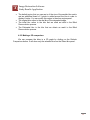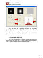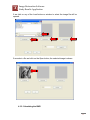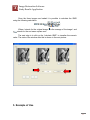
1
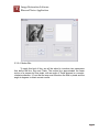
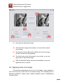
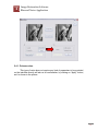
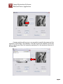
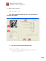
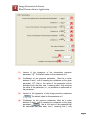
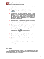
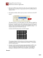
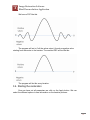
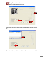
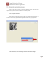
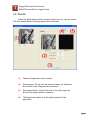
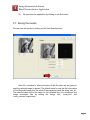
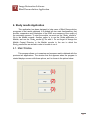
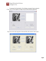
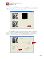
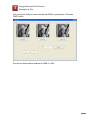
2007 Cora Beatriz Pérez Ariza
José Manuel Llamas
Sánchez
[IMAGE RESTORATION
SOFTWARE.]
Blind Image Deconvolution
User Manual
Version 1.0
*
Image Restoration Software.
Table of Contents Page
1. Introduction
………………………………………………. 4
1.1. Purpose
of
this ………………………………………………. 4
document
2. Blur
and
Noise ………………………………………………. 5
Application
………………………………………………. 5
2.1. Main Window
2.2. Load an Image
………………………………………………. 6
2.3. Blurring the selected ………………………………………………. 8
Image
………………………………………………. 8
2.3.1. Load Blur
2.3.2. Generate Blur
………………………………………………. 10
2.3.2.1. Gaussian
Blur
2.3.2.2. Uniform
Blur
2.3.2.3. Custom
Blur
2.3.2.4. Motion
Blur
2.3.3. Situation after
Blur application
2.4. Applying noise to an
Image
2.4.1. Poisson Noise
………………………………………………. 11
2.4.2. Additive
Gaussian Noise
2.4.3. Multiplicative
Gaussian noise
2.4.4. Situation after
noise application
2.5. Saving Results
………………………………………………. 16
………………………………………………. 12
………………………………………………. 12
………………………………………………. 13
………………………………………………. 14
………………………………………………. 15
………………………………………………. 15
………………………………………………. 17
………………………………………………. 18
………………………………………………. 18
2.6. Closing
the ………………………………………………. 20
Application
3. Blind
Deconvolution ………………………………………………. 21
Application
………………………………………………. 21
3.1. Main Window
2
*
Image Restoration Software.
Table of Contents 3.2. Load an Image
………………………………………………. 22
3.3. Parameters Window
………………………………………………. 26
3.3.1. General
Description
3.3.2. Blind
Deconvolution
Parameters
3.3.3. Options
3.3.4. Advanced
Options
3.4. Starting
Restoration
………………………………………………. 26
………………………………………………. 27
………………………………………………. 29
………………………………………………. 30
the ………………………………………………
3.5. During
the
Restoration Process
3.5.1. No
Option
Selected
3.5.2. Show
Blur,
Noise,
Image
Variance
and
Restored Image
3.5.3. Show
Log
Panel
option
selected
3.5.4. Create Log File
option selected
3.6. Results
3.7. Saving the Results.
32
.
………………………………………………. 33
………………………………………………. 33
………………………………………………. 34
………………………………………………. 34
………………………………………………. 35
………………………………………………. 36
………………………………………………. 37
4. Study
Results ………………………………………………. 39
Application.
………………………………………………. 39
4.1. Main Window
………………………………………………. 40
4.2. Blur Comparison
4.2.1. Loading Blurs
………………………………………………. 41
4.2.2. Making
3D ………………………………………………. 42
comparison
4.2.3. Modifying the ………………………………………………. 43
shown region
………………………………………………. 45
4.3. Image Comparison
4.3.1. Loading
images
the ………………………………………………. 46
3
*
Image Restoration Software.
Table of Contents 4.3.2. Calculating the ………………………………………………. 47
ISNR
………………………………………………. 48
5. Example of Use
6. Authors
of
Document
7. Bibliography
this ………………………………………………. 52
………………………………………………. 53
4
1
Image Restoration Software.
Introduction 1. Introduction
As part of the Computer Engineering Final Project, supervised by Prof.
Rafael Molina in collaboration with Dr. Javier Mateos, members of the
Department of Computer Science and Artificial Intelligence (CCIA) at the
University of Granada (Spain), we have developed a software package that is
able to perform Blind Deconvolution using a variational approach to parameter,
image and blur estimation [1]. This software is divided into three modules: the
first one degrades a given original image, applying blur and noise to it. The
second module actually performs the Blind Deconvolution. The third gives useful
information about the deblurring process, such as the improvement in signal-tonoise ratio (ISNR) as an objective measure of the process quality.
1.1. Purpose of this Document
The aim of this document is to easily explain how each of the modules
works, so it would be easy for anyone to use them. Each and every one of the
features the programs allow us to use will be explained here step by step using
many pictures and diagrams.
First of all, the Noise and Blur application will be explained with a series of
snapshots of the program itself, and all the menus and functionalities will be
shown.
Secondly, the main program will be explained in a similar fashion,
covering the full functionality of the Blind Deconvolution Algorithm developed.
The third part stands for a brief explanation of the last module, so it can
make clear its purpose and functionality, and instructions for use will be given as
well.
The last part of this document contents an example of use that may assist
a first-time user of the application.
5
2
Image Restoration Software.
Blur and Noise Application 2. Blur and Noise Application
This application performs the functionality to degrade an image with blur
and noise determined by the user. To start the module, we must run the
“BlurAndNoise.m” file in the Matlab console. Another option is to run the Guide
application in Matlab, and run the “BlurAndNoise.fig” file with it. Do not forget to
change the Matlab Current Directory in the Matlab console to the one in which
the BlurAndNoise files are stored in order to be able to run it.
The following sections show how to use the program and describe the
functionalities implemented on it.
2.1. Main Window
Here we can see what the program Blur and Noise looks like when it is
started, and a brief explication is given of the main buttons and menus:
6
2
Image Restoration Software.
Blur and Noise Application (1)
The Load Original Image button allows us to load an image
from within the system, in order to work with it.
(2)
This space will display the image we loaded before.
(3)
The Blur panel allows user to apply a blur mask to the loaded
image.
(4)
The Noise panel allows user to apply noise to the previously
blurred image.
(5)
This space will show the observed image, first the blurred
image and later, if this is the case, the blurred and noisy
image.
The Save Degraded Image button allows us to save the
observed image in the system.
(6)
(7)
The Exit button closes the application.
2.2. Load an Image
First thing we need to start working in order to obtain an observed image
is to load an image, so we click on the Load an Image button as it is shown in the
picture:
7
2
Image Restoration Software.
Blur and Noise Application Then we will need to select and open an image using the browser that
pops up. We are able now to search the system looking for an image to degrade.
When the image is found, the next step is to click on the button “Open” in the
browser, as it is shown in the picture:
8
2
Image Restoration Software.
Blur and Noise Application When selected, the image will be shown in the left square of the interface,
looking like this:
Note that the button “Next” is now available in the Blur panel, so we are
now able to start working on the image.
2.3. Blurring the selected Image
We are now going to use the Blur panel to blur the loaded image. The
panel gives us two options:
2.3.1. Load Blur
This option allows us to choose a blur mask stored in a .mat file to apply it
to the loaded image. It must be taken into account that the blur kernel must be
stored in the first variable stored in the .mat file. If the file in question has been
saved with the Blur and Noise application, there will be no problem loading it. We
have to click on the Next button while the Load Blur option is selected, as it is
shown in the next picture. The center of the blur is the center of the mask.
9
2
Image Restoration Software.
Blur and Noise Application Next thing we have to do is select the desired blur mask using the browser
that comes up, and click on ”Next” button on the Blur panel:
10
2
Image Restoration Software.
Blur and Noise Application After this the program will give us the option to apply the selected mask, or
to go back to the main window and start again the blurring process:
11
2
Image Restoration Software.
Blur and Noise Application If we choose to Apply, the blurred image will be shown in the right white
square, showing that blur has been applied successfully.
2.3.2. Generate Blur
In case we want to generate a blur mask instead of loading it from a file,
we have to select the Generate Blur option as it is shown in the picture:
The interface will show the four possibilities we have for blur: which are
Gaussian, Uniform, Customized and Motion, and user should select one and
then click on “Next” button.
12
2
Image Restoration Software.
Blur and Noise Application 2.3.2.1. Gaussian Blur
To apply this blur, we will be asked to introduce two parameters that
define the blur: Size and Sigma2. This creates a [Size x Size] Gaussian kernel
filter with variance value of Sigma2:
13
2
Image Restoration Software.
Blur and Noise Application 2.3.2.2. Uniform Blur
This blur requires a parameter that is the size of the blur kernel, and so
the interface will ask us for it:
2.3.2.3. Customized Blur
This option gives us the possibility to configure a blur kernel according to
our own preferences, giving us a 7x7 matrix to specify it. The kernel must be
centered in the middle of the square (4th row, 4th column).
14
2
Image Restoration Software.
Blur and Noise Application 2.3.2.4. Motion Blur
To apply this kind of blur, we will be asked to introduce two parameters
that define the blur: Size and Theta. The motion blur approximates the linear
motion of a camera by Size pixels, with an angle of Theta degrees in a counterclockwise direction. It is so that the user must introduce the Size in pixels and the
angle in degrees to obtain correct results:
15
2
Image Restoration Software.
Blur and Noise Application 2.3.3. Situation after blur application.
After any of the Blur types have been applied, we will show the main Blur
panel view again. In the next picture we give details about the new situation:
16
2
Image Restoration Software.
Blur and Noise Application (1)
Here we have the blurred image.
(2)
This Show Blur Image button allows us to see the blur matrix
as an image.
(3)
The Remove Current Blur button deletes blur from the image
and lets us start from the beginning.
(4)
The Next button in the Noise panel is now active, so we can
apply noise to the blurred image.
(5)
With the Save Blur button we have the possibility to save the
applied blur into a .mat file.
2.4. Applying noise to an image.
The second transformation we can do to the image is noise application.
We now show how to add noise to the blurred image. The interface gives us
different possibilities: Poisson noise, Additive Gaussian noise or Multiplicative
Gaussian noise.
17
2
Image Restoration Software.
Blur and Noise Application 2.4.1. Poisson noise.
This type of noise does not require any kind of parameters to be provided,
so the interface directly will ask us for confirmation, by clicking on “Apply” button,
as it is shown in the picture:
18
2
Image Restoration Software.
Blur and Noise Application After pressing “Apply”, the right image window will be updated with the
desired noise added to the blurred image.
2.4.2. Additive Gaussian noise.
In order to introduce this kind of noise, we will be asked to provide the
noise variance or the signal-noise ratio. If we press the Enter key in our keyboard
after introducing any of the parameters, the other will be automatically actualized,
so we will see if the noise is the one desired before actually applying it:
19
2
Image Restoration Software.
Blur and Noise Application 2.4.3. Multiplicative Gaussian noise.
This type of noise requires the parameter that multiplied by the blurred
observation corresponds to the variance of the noisy observation, so it will be
requested through the interface as it is shown below:
20
2
Image Restoration Software.
Blur and Noise Application 2.4.4. Situation after noise application.
After applying any noise to the blurred image, the interface will look like
the image below. Note that we will not be able to introduce any other kind of
noise into the image unless the “Remove Current Noise” button is clicked on, in
that case the interface will delete the current noise and we will be able to start
from the beginning of the noise-application process.
2.5 Saving Results.
We are able to save the degraded image at any time in the degradation
process, only by pressing the “Save Degraded Image” button, as it is shown in
the picture. Keep in mind that the image being saved is the one showed in the
right square of the interface:
21
2
Image Restoration Software.
Blur and Noise Application A saving window will pop up so we are able to specify the name and the
extension of the image. The extension .mat will be given as a default, but we are
able to specify any other file format by specifying it in the window at the end of
the file name.
22
2
Image Restoration Software.
Blur and Noise Application 2.6. Closing the application.
To close the application and all its windows, we just have to press the
“Exit” button, as it is shown in the picture:
23
3
Image Restoration Software. Blind Deconvolution Application
3. Blind Deconvolution Application
This application implements the Blind image restoration method proposed
in [1]. To start the module, we must run the “Blind_deconvolution.m” file in the
Matlab console. Another option is to run the Guide application in Matlab, and run
the “Blind_deconvolution.fig” file with it. Do not forget to change the Matlab
Current Directory in the Matlab console to the one in which the
Blind_deconvolution files are stored in order to be able to run it.
3.1. Main Window
Here we can see what the program looks like when it is started, and a brief
explanation is given of the main buttons. In this step we must load an Observed
Image, an Initial Image and the Initial Blur for the Blind Deconvolution process:
24
3
Image Restoration Software. Blind Deconvolution Application
(1)
The “Load Observed Image” button allows us to load an
image from within the system which will be the degraded
Observed Image.
(2)
The “Load Initial Image” button allows us to load an image
from within the system which will be the Initial Image for the
restoration process.
(3)
The “Load Initial Blur” button allows us to load an image from
within the system which will be the Initial Blur for the
restoration process.
(4)
The “Exit” button closes the application.
(5)
The “Next” button takes us to the next window of the
application in which we can set up the parameters for the
Blind Deconvolution process.
(6)
The “Reset” button takes us to the main window of the
application.
3.2. Load an Image
First we click on the Load Observed Image button in order to load the
image we want to restore.
25
3
Image Restoration Software. Blind Deconvolution Application
Then we will need to select and open a picture using the browser that
pops up. Allowed file formats are .mat and common image formats like .bmp, .tif,
.png, .gif or .jpg. When the image is selected, the next step is to click on the
button “Open” in the browser, as it is shown in the picture:
26
3
Image Restoration Software. Blind Deconvolution Application
When selected, the image will appear in the square over the button. By
default, the Initial Image for the restoration process will be the same image, and
the Initial Blur will be a Gaussian Blur with deviation Sigma=2. The size in pixels
of the Observed Image is shown below the image:
27
3
Image Restoration Software. Blind Deconvolution Application
We can load a different Initial Image by clicking on the Load Initial Image
button:
28
3
Image Restoration Software. Blind Deconvolution Application
We can load a different Initial Blur by clicking on the Load Initial Blur
button:
To go to the next step we must click on the Next button:
29
3
Image Restoration Software. Blind Deconvolution Application
3.3. Parameters Window
3.3.1. General Description
Here we can see what the window looks like. A brief description now is
given of the main elements:
(1)
Here we can see the Observed Image and its size.
(2)
The “Options” Panel has different options that we can choose
to show information of the restoration process. For further
information see chapter 3.3.3.
30
3
Image Restoration Software. Blind Deconvolution Application
(3)
The “BD Parameters” panel has fields with the different
parameters which are used by the Blind Deconvolution
algorithm. For further information see chapter 3.3.2.
(4)
The “Back” button takes us to the previous window of the
application.
(5)
The “Apply” button starts the Blind Deconvolution process with
the selected parameters and options.
3.3.2. Blind Deconvolution Parameters
Here we can see the different parameters and a short description of each
of them:
31
3
Image Restoration Software. Blind Deconvolution Application
(1)
Inverse of the hyperprior of the observation precision
0
parameter 1/β . The default value for this parameter is 0.
(2)
Confidence on the previous parameter. Must be a value
between 0 and 1, with 0 meaning no confidence on the given
0
parameter 1/β , that is, the value of the parameter will be
estimated from the data, and 1 meaning that it fully enforces
the value of the parameter, i.e., no estimation is performed on
the parameter.
(3)
Inverse of the hyperprior of the Image precision parameter
The default value for this parameter is 0.
(4)
Confidence on the previous parameter. Must be a value
between 0 and 1, with 0 meaning no confidence on the given
parameter
, that is, the value of the parameter will
be estimated from the data, and 1 meaning that it fully
32
3
Image Restoration Software. Blind Deconvolution Application
enforces the value of the parameter, i.e., no estimation is
performed on the parameter.
(5)
Inverse of the hyperprior of the Blur precision parameter
. The default value for this parameter is 0.
(6)
Confidence on the previous parameter. Must be a value
between 0 and 1, with 0 meaning no confidence on the given
parameter
, that is, the value of the parameter will
be estimated from the data, and 1 meaning that it fully
enforces the value of the parameter, i.e., no estimation is
performed on the parameter.
(7)
Maximum number of iterations of the algorithm. The process
stops if the stopping criterion is met. If not it stops when it
reaches the maximum number of iterations.
(8)
Stopping criterion. The algorithm stops if the result of divide
the norm of the difference between the restored image of the
actual iteration and the restored image in the previous
iteration by the norm of the restored image of the actual
iteration is less than this value.
(Mathematically:
(9)
Stopping criterion)
Prior model of the image and the blur. We can choose
between a Simultaneous Auto-Regressive prior model and a
Conditional Auto-Regressive prior model.
(10) Distribution of the image and the blur. We can choose
between:
- Both deterministic.
- Deterministic distribution of the blur and Random distribution
of the image.
- Both Random.
3.3.3. Options
The options of this panel enable us to see information about the Blind
Deconvolution process. We can run the Blind Deconvolution method without any
log information or select one or more options.
33
3
Image Restoration Software. Blind Deconvolution Application
(1)
With this option the application displays the image, blur and
noise variance and it also shows you the restored image. This
information is refreshed every given number of iterations. See
(2).
(2)
Number of iterations to refresh the information in (1).
(3)
With this option the application creates a panel where all the
information that the application generates during the
restoration process is displayed.
(4)
With this option the application creates a file where all the
information that the application generates during the
restoration process is stored.
3.3.4. Advanced Options
This panel inside the Option panel allows us the possibility of choosing
between three different PSF sizes.
34
3
Image Restoration Software. Blind Deconvolution Application
•
Full size: the PSF support will be the same size of the image during the
Blind Deconvolution process. Components of the PSF could be positive or
negative values.
•
Set (height and width): with this option you have to set the size of the PSF
support.
This option will set to 0 all the values of the PSF that are outside the
kernel size. The default value is [20 x 20]. Components of the PSF could
be positive or negative values, but normalization is applied to the PSF in
order to keep its components (positives and negatives) making 1. An
example is given here to illustrate the process:
If we have this PSF and we select a 4x4 PSF support:
0
0
0
0
0
0
0
0
0
0
0
0
0
0
0
0
0 0 0 0 0
0 0 0 0 0
0
0
0
0
0 0 0 0 0
0 0 0 0 0
0
0
0
0
0
0
0
0
The program will set to 0 all the values out of the grey squares and then
normalize all the PSF in order to keep the values making 1. The program
will do this each iteration.
•
Automatic: with this option the program sets automatically the PSF. It sets
to 0 all the values from the border of the PSF until it founds a negative
value, so no negative value will remain in the support. Here again it is
necessary to normalize the PSF in order to keep the values making 1.
Example:
35
3
Image Restoration Software. Blind Deconvolution Application
We have a PSF like this.
The program will set to 0 all the values since it founds a negative value
starting from the center to the borders. The resulted PSF will be like this:
The program will do this every iteration.
3.4. Starting the restoration
Once we have set all parameters we click on the Apply button. We can
select the different options to see information on the iterative process:
36
3
Image Restoration Software. Blind Deconvolution Application
If we choose the Create a log file option a window to select the output file pops
up:
We must write the name that we want for the log file and click on the save button.
37
3
Image Restoration Software. Blind Deconvolution Application
3.5. During the restoration process
Here we will see the result of choosing different options. We show the
options one by one but we can combine two or more options.
3.5.1. No option selected
After clicking on the Apply button we will see a window with information. If
we did not choose any option then the application shows only a progress bar:
3.5.2. Show blur, noise and image variance and restored image
38
3
Image Restoration Software. Blind Deconvolution Application
If this option is selected we will see some information and the progress
bar. The window will look like the one below:
The information that we see is the noise, image and blur estimates and the
restored image. This information is refreshed every the set number of iterations
that we specified on the options on the previous window.
3.5.3. Show Log Panel option selected
If this option is selected more information will be shown than with the
previous option and the progress bar. The window will have this aspect:
39
3
Image Restoration Software. Blind Deconvolution Application
3.5.4. Create a Log file option selected
If this option was selected a log file will be created. The log file is a .txt file
with information. A typical log file is shown below:
40
3
Image Restoration Software. Blind Deconvolution Application
3.6. Results
When the Blind Deconvolution process finishes we can see the results.
This final window has the following aspect and functionality:
(1)
Observed image and its size in pixels.
(2)
Results panel. We can see the restored image, the estimated
blur and the noise, image and blur estimates.
(3)
Save results button. It allows the user to save the image, the
blur and the image and blur covariance.
(4)
The Reset button takes us to the starting window of the
application.
.
41
3
Image Restoration Software. Blind Deconvolution Application
(5)
We can leave the application by clicking on the Exit button.
3.7. Saving the results
We can save the results by clicking on the Save Results button:
After this, a window to select the name of the file where we are going to
save the restored image is opened. The default name to save the file is the name
of the Observed image plus the value of the parameters and the string ‘rest_im’.
The selected name will be the same for the obtained blur, blur covariance and
image covariance files by adding the strings ‘blur’, ‘covar_blur’ and
‘covar_restored’ respectively.
42
3
Image Restoration Software. Blind Deconvolution Application
Here we can see the saved files with their names.
43
3
Image Restoration Software. Blind Deconvolution Application
4. Study results Application
This application has been designed to help users of Blind Deconvolution
processes to test results obtained. It is divided into two main functionalities, that
are Blur comparison and Calculation of the ISNR as a measure of the quality of
the restoration process. To start the module, we must run the “Study_results.m”
file in the Matlab console. Another option is to run the Guide application in
Matlab, and run the “Study_results.fig” file with it. Do not forget to change the
Matlab Current Directory in the Matlab console to the one in which the
Study_results files are stored in order to be able to run it.
4.1. Main Window
This program allows us to examine and compare results obtained with the
previous two applications. The window that first appears when the program is
started displays a menu with three options, as it is shown in the picture below:
44
4
Image Restoration Software.
Study Results Application (1)
The Blur button takes us to the blur window. In that window
we can load different blurs and see the differences between
them.
(2)
The Image button takes us to the image window. In that
window we can load three images, show them and calculate
the ISNR.
(3)
The Exit button closes the application.
4.2. Blur Comparison
It is shown here the blur window appearance and a brief explanation of the
main buttons is also given:
(1)
There are three areas where you can load different blurs. You
will see the size of each blur in pixels in the white rectangles.
45
4
Image Restoration Software.
Study Results Application (2)
The show region panel allows you to make zoom in or zoom
out in the blurs.
(3)
This panel allows you to select the blur or blurs that you want
to plot (see 4).
(4)
Here is where the application shows the 3D graph of the
selected blurs when you click on the refresh comparison
button.
(5)
The back button takes you to the main window of the
application.
(6)
The exit button closes the application.
(7)
The Refresh Comparison button shows a 3D graph with the
selected blurs in the graphics region (see 3 and 4).
4.2.1. Loading the blurs
If we click on any of the Load buttons a window to select the blur file will be
opened.
46
4
Image Restoration Software.
Study Results Application If we select a file and click on the Open button the blur and its size are shown.
47
4
•
•
•
•
Image Restoration Software.
Study Results Application The default region that you can see is of the size of the smaller blur matrix
and an additional frame of 3 pixels is added around the blur in order to
display it better. You can modify this region in the show region panel.
The original blur refers to the real blur of the degraded image.
The initial blur refers to the blur that we used as initial in the Blind
Deconvolution process.
The Estimated blur is the blur that we obtain as result in the Blind
Deconvolution process.
4.2.2 Making a 3D comparison
We can compare the blurs in a 3D graph by clicking on the Refresh
Comparison button. It will show only the selected blurs on the Select blur panel.
48
4
Image Restoration Software.
Study Results Application As we can clearly see in the picture, each three blur functions are
superposed in a three-dimensional plot to allow us to compare the blurs in every
direction. Black color stands for the Original Blur, red for the estimated Blur and
Green for the Initial Blur used in the Blind Deconvolution process.
We are able to rotate the 3D graph by moving the mouse pointer while the
left button is pressed.
4.2.3 Modifying the shown region
We can also zoom in or zoom out the blurs using the panel shown in the
next picture. We can set the size of the region by setting its height and width.
Then, if we click on the Apply button, the new region is shown.
49
4
Image Restoration Software.
Study Results Application Note that the new psf regions will not be displayed in the 3D plot until we
click on the Refresh Comparison button.
4.3. Image comparison
50
4
Image Restoration Software.
Study Results Application Here we can see what the image comparison window looks like and a
brief explanation of the main buttons.
(1)
By clicking on the “Load Original Image” we are able to select
a picture that represents the original image.
(2)
By clicking on the “Load Blurred Image” we are able to select
a picture that represents the observed image.
(3)
By clicking on the “Load Restored Image” we are able to
select a picture that represents the restored image.
(4)
The Calculate ISNR button allows you to calculate the ISNR
of the restored image.
(5)
The back button takes you to the main window of the
application.
(6)
The exit button closes the application.
4.3.1. Loading the images
51
4
Image Restoration Software.
Study Results Application If we click on any of the Load buttons a window to select the image file will be
opened.
If we select a file and click on the Open button, the selected image is shown.
4.3.2. Calculating the ISNR
52
4
Image Restoration Software.
Study Results Application Once the three images are loaded it is possible to calculate the ISNR
using the following calculation:
.
Where I stands for the original image,
stands for the root mean square error.
is the average of the image I and
The next step is to click on the “calculate ISNR” to visualize the numeric
value. The state of the window after this is shown in the next picture:
5. Example of Use
53
5
Image Restoration Software.
Example of Use To represent the functionality of the software, we present here an example
of use: First of all we degrade an image using the BlurAndNoise application:
Then we convolve the image with a Gaussian Blur with variance 5 and size 25:
54
5
Image Restoration Software.
Example of Use Then we add additive Gaussian noise with variance 4 and save the
degraded image and the blur. Now we start the Blind Deconvolution application
and load the degraded image we have just created:
We can keep the default initial blur and image given by the program. Now
we click on “Next” button and proceed to set the parameters for example the
number of iterations equal to 3 and for the rest of parameters we use the default
options. In the advanced options we set the PSF support to automatic:
55
5
Image Restoration Software.
Example of Use Now we press Apply and start the Blind Deconvolution process. At the end
of the restoration, we see the following screen:
Finally we analyze the restored image and the estimated psf using the
third application “Study Results”. We start by visualizing the blur images:
56
5
Image Restoration Software.
Example of Use Now, and just to finish, we can calculate the ISNR by pressing the “Calculate
ISNR” button:
We can see that we have obtained an ISNR of 1.446.
57
6
Image Restoration Software.
Authors of this Document 6. Authors of this Document
José Manuel Llamas Sánchez
Cora Beatriz Pérez Ariza
58
59
7
Image Restoration Software.
Bibliography 8. Bibliography
[1]
[2]
R. Molina, J. Mateos and A. K. Katsaggelos “Blind Deconvolution using a
variational approach to parameter, image, and blur estimation,” IEEE
Trans. on Image Processing, vol. 15, no. 12, 3715-3727, December
2006.
S. Derin Babacan, R. Molina, A. K. Katsaggelos “Total Variation Blind
Deconvolution Using a variational approach to parameter, image and blur
estimation”
[3]
P. Campisi, K. Egiazarian “Blind image deconvolution: Theory and
Applications” CRC Press, 2007
[4]
R. Molina, “Introducción al Procesamiento y Análisis de Imágenes
Digitales,” curso impartido en Introducción a la Robótica hasta 1998,
Dpto. de Ciencias de la Computación e I.A., Universidad de Granada.
[5]
T. Bishop, D. Barbacan, B. Amizic, T. Chan, R. Molina, and A. K.
Katsaggelos, “Blind Image Deconvolution: problem formulation and
existing approaches”, in Blind image deconvolution: Theory and
Applications, P. Campisi, and K. Egiazarian (ed.), CRC, 2007.