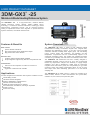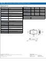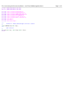
1
Mobile Robotics in Precision Agriculture A CAN bus interface implementation of differential drive and exploration of localization, pose estimation and autonomous navigation. Torgrim Aalvik Lien Master of Science in Engineering Cybernetics Submission date: July 2013 Supervisor: Jan Tommy Gravdahl, ITK Co-supervisor: Trygve Utstumo, Adigo AS Norwegian University of Science and Technology Department of Engineering Cybernetics NTNU Norges teknisk-naturvitenskapelige universitet Fakultet for informasjonsteknologi, matematikk og elektroteknikk Institutt for teknisk kybernetikk Master thesis Name of the candidate: Subject: Title: Torgrim Aalvik Lien Engineering Cybernetics Mobile Robotics in Precision Agriculture A CAN bus interface implementation of differential drive and exploration of localization, pose estimation and autonomous navigation. Background: Adigo AS is a research partner in the consortium project "Multi-sensory Precision Agriculture"1, and develop a mobile field robot. The robot has differential drive with two 5kW brushless DC motors and SevCon Gen4 motor controllers with a CAN Open based interface. The robot will be equipped with a GPS and an IMU (Inertial Measurement Unit) for localization and pose estimation. The software architecture of the robot is built on top of ROS2. The project has two main goals: Develop an interface from ROS to the CANopen motor-controllers, and move towards autonomous navigation with waypoint following. Differential drive and CanOpen interface 1. Build a lab setup with two motors and controllers communicating on the same CAN-bus. 2. Control the motors directly by an analogue input, and direct CANopen commands. 3. Develop a ROS package with a node for the motor-controller. 4. Implement and demonstrate differential drive in the lab. 5. Implement and test the differential drive controller on the field robot. Autonomous Waypoint Navigation 1. Present a brief overview of localization, pose estimation, path-planning for non-holonomic vehicles and path following. 2. Implement and test the GPS receiver with ROS. 3. Implement and test the IMU sensor with ROS. 4. Demonstrate localization and pose estimation. 5. Implement a path-planning algorithm 6. Perform a demonstration of autonomous waypoint navigation. The laboratory experiments will be performed at NTNU in cooperation with Adigo, and field test and full scale experiments will be performed at Adigo in Oppegård. External advisor: Trygve Utstumo, Adigo AS Project assigned: January, 2013 To be handed in by: June, 2013 Trondheim, January 2013 Jan Tommy Gravdahl Professor, supervisor 1 2 The Norwegian Research Council, Application number: ES464593 Multisensory precision agriculture - improving yields and reducing environmental impact (Researcher project – MATPROGRAMMET) Robotic Operating System, www.ros.org II Abstract A complete setup of sensors, estimators and controllers for autonomous and manual control of an unmanned differential steered ground vehicle has been implemented in this paper. The entire system is implemented in Robot Operative System (ROS) using the open source ROS software platform FroboMind as a foundation. The system is running on a Ubuntu 12.10 laptop, with the Groovy distribution of ROS. A reliable CANopen communication for real-time control and monitoring of the motors over a single CAN bus have been deployed, with security measures for handling loss of connection between the motor controllers and the computer. Pose and position estimation using sensor data from wheel odometry, IMU sensor input and GPS signals has been implemented in an extended kalman filter. A scheme for waypoint navigation for has been deployed, with a slow control loop for calculation of a manifold to ensure that the vehicle reaches the waypoint with the right heading, and a fast subsystem ensuring that the robot follows the manifold. Due to inaccuracy of the compass and the IMU, the position and pose estimator struggles a bit with the heading accuracy. This can be improved greatly by a better calibration of the IMU. Since we are using a stand alone GPS receiver, the accuracy of the position is in the range 2-3 meters, the accuracy of the estimators can not be more accurate. By using another GPS receiver as a base unit, the accuracy may be improved to a few cm. The waypoint navigation works really well until the vehicle is close to the waypoint, where the inaccuracies of the position estimator leads to big changes in the parameters in waypoint navigation algorithm. This is III IV solved by introducing a parking algorithm that ensures a smooth parking of the vehicle. Sammendrag En platform av sensorer, estimatorer og kontrollere for både autonom og manuell styring av et ubemannet bakkekjøretøy (UGV) har blitt implementert i denne oppgaven. Hele systemet er implementert i Robot Operative System(ROS). Programpakken FroboMind, et sett av åpen kildekode ROS programmer laget for feltroboter har blitt brukt som fundament for systemet. Systemet kjører på en Ubuntu 12.10 laptop, med Groovy ditribusjonen av ROS. En pålitelig CANopen kommunikasjon mellom to motorkontrollere og datamaskinen med sikkerhetsprosedyrer for håndtering av brudd i kommunikasjonen CAN bus er opprettet. All CAN kommunikasjon foregår over en enkelt CAN bus. Informasjon fra en GPS mottaker, kompasset i en IMU-enhet og målinger av hastighet fra hjulene kombineres i et ulineært Kalman filter for estimasjon av kjøretøyets posisjon,hastighet og retning. Autonom kontroll av kjøretøyet er implementert i en rutepunktsnavigasjonsalgoritme. Algoritmen består av to kontrolløkker,en treg kontroller som regner ut et manifold som sikrer at kjøretøyet når rutepunktet. Og en raskere kontroller som regner ut krummingen på veibanen til kjøretøyet som sikrer at kjøretøyet følger manifoldet inn til rutepunktet. Det er altså ikke snakk om å planlegge en optimal rute, for så å følge den, men heller å bruke vektorfelt som ”dytter” kjøretøyet i mål. Da det kun brukes en GPS mottaker uten noen form for korreksjon her, er nøyaktigheten på posisjonen såpass lav at usikkerheten til posisjonen blir på flere meter. For praktisk bruk, må en form for korreksjon implementeres. Kalibrering av IMU-enheten har også vist seg å være vanskelig, da det er mange elementer på kjøretøyet som forstyrrer jordens magnetfelt. Dette gjør at Kalmanfilteret sliter litt med retningsestimatet når V VI kjøretøyet svinger, men det korrigerer seg fort etter å ha kjørt rett fram noen meter. Rutepunktsnavigasjonen fungerer godt når avstanden til rutepunktet er stor, men jo nærmere målet en kommer, jo større innvirkning på kontrolleren har unøyaktighetene fra posisjons- og retningsestimatet. Dette har blitt løst ved å introdusere en egen parkeringsalgoritme som tar over når kjøretøyet er under 1 meter fra rutepunktet. Preface There are many people who deserves my deepest gratitude for the help offered on this project. I would like to start by thanking my co-supervisor Trygve Utstumo at Adigo, for always being available to assist me and being a good friend. I have spent several weeks working in the offices at Adigo, and I am really grateful for the way everyone there has made me feel welcome. Lars Molstad deserves my thanks for providing me with a place to work and do field tests at the Norwegian University of Life Sciences in Aas. Kjeld Jensen at the University of Southern Denmark, has offered great assistance in implementation of FroboMind, he deserves my thanks, both for the assistance he has provided me, and for developing a great open source platform that I have found very helpful. Jan Tommy Gravdahl, my supervisor here at NTNU also deserves my gratitude. His calm nature has really helped in what would normally be a stressful period. I have always felt more calm and confident after our meetings, even when he has stressed that i should start writing some more on my paper. VII VIII In loving memory of Egil Lien X Contents 1 Introduction 1 2 Theory 2.1 Mathematical modeling . . . . . . . 2.2 CANopen protocol . . . . . . . . . . 2.3 Vehicle location and pose estimation 2.4 Waypoint Navigation . . . . . . . . . 3 Hardware 3.1 MotEnergy ME0970 electric motor 3.2 Sevcon gen4 motor controller . . . 3.3 Septentrio polaRx2 gps receiver . . 3.4 Microstrain 3DMG-GX3-25 IMU . . . . . . . . . . . . . . . . . . . . . . . . . . . . . . . . . . . . . . . . . . . . . . . . . . . . . . . . . . . . . . . . . . . . . . . . . . . . . . . . . . . . . . . . . . . . . . . . . . . . . . . . . 3 3 5 12 16 . . . . 19 19 19 21 21 4 Software 23 4.1 ROS . . . . . . . . . . . . . . . . . . . . . . . . . . . . . . . 23 4.2 FroboMind . . . . . . . . . . . . . . . . . . . . . . . . . . . 24 5 Implementation 5.1 CAN communication . . . . . . . . . 5.2 Laboratory Setup . . . . . . . . . . . 5.3 ROS implementation . . . . . . . . . 5.4 Vehicle pose and position estimation 5.5 Waypoint Navigation . . . . . . . . . . . . . . . . . . . . . . . . . . . . . . . . . . . . . . . . . . . . . . . . . . . . . . . . . . . . . . . . . . . . . . . . . . 27 27 27 28 28 32 6 Results and evaluation 39 6.1 Laboratory setup . . . . . . . . . . . . . . . . . . . . . . . . 39 6.2 CANopen integration . . . . . . . . . . . . . . . . . . . . . . 39 XI XII Contents 6.3 6.4 6.5 6.6 6.7 GPS integration . . IMU integration . . Wheel odometry . . Pose Estimation . . Waypoint Navigation . . . . . . . . . . . . . . . . . . . . . . . . . . . . . . . . . . . . . . . . . . . . . . . . . . . . . . . . . . . . . . . . . . . . . . . . . . . . . . . . . . . . . . . . . . . . . . . . . . . . . . . . . . . . . . 42 42 43 43 43 7 Conclusion 51 7.1 Further Work . . . . . . . . . . . . . . . . . . . . . . . . . . 52 Bibliography 52 Appendix 54 A Data sheets . . . . . . . . . . . . . . . . . . . . . . . . . . . 55 B Header Files . . . . . . . . . . . . . . . . . . . . . . . . . . . 63 Chapter 1 Introduction As a part of the consortium project ”Multi-sensory Precision Agriculture” 1 Adigo A/S works with Bioforsk and The University in Aas on a unmanned ground vehicle for effective N2O-measurements. The UGV measures N2O emissions by soil cover methods. Traditional soil cover methods are labourous and requires a lot of big instruments. Hence robotic solutions are needed for the project. Adigo has developed a UGV made for holding all the sensory equipment for measuring N20 emissions. Before this project started the robot was controlled manually by an operator with a joystick connected directly to the motor controllers of the vehicle. In order to make a unmanned vehicle, the control of the vehicle is to be done via the CAN interface of the controller. To monitor position, orientation and speed of the vehicle, along with data from the wheel odometry, available sensors are a Septentrio PolaRx2 gps receiver and a Microstrain 3DM-GX3 inertial measurement unit. In this project a system for controlling the vehicle both manual via an wireless Xbox 360 controller and autonomous via a waypoint finding algorithm will be implemented. All software will be implemented in ROS, an open source pseudo operative system for robotic applications. FroboMind, a set of open source ROS packages made for field robots developed at the University of Southern Denmark and other universities and companies in Denmark, will be used as a platform for the system. As a core of the system a ROS node for handling transmission and 1 The Norwegian Research Council, Application number: ES464593 Mutisensory precision agriculture - improving yields and reducing environmental impact (Researcher project - MATPROGRAMMET 1 2 Chapter 1: Introduction reception of CANopen messages from the motor. The motor controllers are set to control the motors via an internal PI loop for controlling the speed directly, so for controlling the motors, our system will send reference speeds to the controllers. The reference speeds are either decided by an input from the joystick or by a waypoint navigation controller. For position estimation an extended Kalman filter, combining measurements from wheel odometry, gps and IMU will be implemented. The waypoint navigation algorithm used is an algorithm that calculates the curvature of the path to follow according to the position and orientation of the vehicle relative to the position and orientation of the waypoint. It does not plan a path and tries to follow this path, rather it follows a manifold leading to the waypoint. Testing of the system will be made at the Norwegian University of Life Sciences in Aas. This project is a built on a previous project ”Motor Control For Precision Agriculture - A CAN bus interface implementation”(Lien, 2012). Chapter 2 Theory 2.1 2.1.1 Mathematical modeling Kinematic model of the vehicle The differential steered vehicle is simple in its dynamics. The two driving wheels move independent of each other and the rate of turning is decided by the difference in speed of the two wheels. The kinematics of the vehicle is straight forward vright − vlef t dwheels (2.1) 1 v = (vright + vlef t ) 2 (2.2) ω= 3 4 Chapter 2: Theory Figure 2.1: Vehicle from above 2.2 CANopen protocol 2.2 5 CANopen protocol CANopen is the internationally standardized (EN 50325-4) CAN based higher-layer protocol for embedded control systems. CAN defines the physical and data layer of OSI level(OSI), CANopen implements the OSI layers from the CAN interface and up to the application layer. The CANopen protocol provides a set of protocols to configure, control and supervise nodes in an embedded network. Figure 2.2: The CANopen protocol covers both the network, transport, session and presentation layer 2.2.1 The CANopen object dictionary The CANopen Object Dictionary is the core of the CANopen protocol. Its basically a grouping of parameters and objects accessible via the network via predefined messages. Each object in the object dictionary is dressed by a 16 bit index and an 8 bit subindex. All writing and reading of parameters 6 Chapter 2: Theory are done via the object dictionary. Making this the interface between the CAN messages and the application interface. Figure 2.3: All parameters are set and read from the CANopen Object Dictionary The object dictionary is divided in several index ranges. Objects in range 0x1000 to 0x1FFF is the same for every CANopen device. This is the communication object area, where parameters for message handling and setup of different CANopen messages are made. Objects in the range 0x2000 to 0x5FFF and 0x6000 to 0x9FFF describe the application behavior of the device, these objects the manufacturers are free to arrange however desirable. Index 0x0000 0x0001-0x025F 0x0260-0x0FFF 0x1000-0x1FFF 0x2000-0x5FFF 0x6000-0x9FFF 0xA000-0xBFFF 0xC000-0xFFFF Description reserved Data Types reserved Communication object area Manufacturer specific area Device profile specific area Interface profile specific area reserved Table 2.1: Index ranges in CANopen Object Dictionaries. 2.2 CANopen protocol 2.2.2 7 Protocols Network management (NMT) protocols A CANopen device can be in four different states; Initialization, PreOperational, Operational and Stopped. To switch between these states a network management state machine is used. The device working as a NMT master sends NMT messages initiating state changes. Support for the NMT slave state machine is a requirement for all CANopen devices. Figure 2.4: NMT state machine The NMT messages uses COB-ID 0x00, giving them the highest priority of all the messages sent on the CAN bus. The NMT message consists of one single CAN data frame containing 2 bytes of data. The first byte holds which state to go to, and the second byte holds which node to respond to the message by changing its state. If the byte identifying the node is set to zero, all the nodes on the network will act upon the message. For creating a safe critical system, heartbeats are set up. The heartbeats are used to check the presence of nodes in the network and to verify that they are working correctly. The heartbeat message are sent cyclic with a predefined time interval from the heartbeat producer, it is assigned 8 Chapter 2: Theory with CAN-identifier 0x700+NodeID and contains one byte of data. The data byte contains the state of the node. The heartbeat consumer has a consumer time gap stored in it dictionary, if the consumer fails to receive a heart beat within this time frame, a event will be generated. Service Data Object (SDO) protocol Service data objects are allowed to access any entry of the CANopen object dictionary. The SDO protocol is a confirmed communication service, which means it is a two-way communication. One SDO consists of two CAN data frames with different CAN-IDs, following a SDO a peer-to-peer client-server connection between two nodes can be established, making it possible to send any number of data in a segmented way. Therefore SDO is primarily used for sending configuration data.The node holding the accessed object dictionary is the server for the SDO. The device accessing the object dictionary is the client. So when sending configuration data from a PC to a CANopen device the device works as a server, and the PC as a client during the SDO. There are three different variants of the SDO protocol; expedited transfer, normal transfer and block transfer. A normal transfer is initiated by a SDO message sending a request to write or read a number of bytes, the node holding the object dictionary written to or read from then sends a response to the request, if granted, segments of 7 bytes will be sent, each segment followed by a confirmation message from the receiver. Confirmation of every CAN message sent takes time, to speed up the transfer of large amounts of data, block transfer may be used. This works as normal a normal transfer, but instead of sending a response to every CAN message containing data, a confirmation will only be sent after a block of data segments (max 127 segments). For small amounts of data, the easiest and quickest way to send data is by expedited transfer. Here the SDO message initiating the connection also transfers the data. In expedited transfer the maximum amount of data sent is 4 bytes. A CANopen device can support up to 128 SDO server channels, and up to 128 SDO client server channel. Each channel may be configured by writing valid COB-IDs to the related SDO parameter set. Each channel holds two COB-IDs, one server-to-client COB-ID and one client to server COB-ID. 2.2 CANopen protocol 9 The parameters of the first SDO server channel is predefined and must be the same for all CANopen devices. This channel uses COBID (0x600+node ID) for client-server and COB-ID (0x580+node ID) for server-client. Process Data Object (PDO) protocol Process Data Objects are short high-priority CAN messages transmitted in a broadcast. These messages are sent in an unconfirmed manner, which means that there is no acknowledgement that the messages has been received by any node in the network (CiA). The high priority of the messages makes the suitable for sending real time data. A PDO message consists of one single CAN frame and is able to send 8 bytes of data. Within these 8 bytes up to 8 data objects can be mapped, depending of the size of the data sent in each mapping. Transmission of PDOs are configured in the Transfer PDO (TPDO) and receive PDO (RPDO) slots in the data object dictionary. When a PDO message is sent the producer sends a message corresponding to the information configured in the TPDO communication and mapping parameters stored in the data object library. If a node is supposed to support reception of this message, the RPDO communication and mapping parameters in the object dictionary of this node is set to recognize the CAN-ID of the message and how the received data is structured and stored in its object dictionary. A PDO can be triggered by different events. It can be triggered by a remote transmission request CAN-message (RTR), a SYNC message or by device-internal events. Remotely triggered PDOs can be triggered by a RTR CAN SYNC triggered messages can be used for sending cyclic data. RPDO communication is arranged in data object dictionary index 0x1400-0x15FF, RPDO mapping is arranged in 0x1600-0x17FF. TPDO communication is arranged in data object dictionary index 0x1800-0x19FF, TPDO mapping is arranged in 0x1A00-0x1BFF. Synchronization Object (SYNC) The synchronization object is message sent periodically to trigger synchronous events. It consists of a single CAN frame with ID 0x80. The purpose of the SYNC message is to trigger messages that are set to send synchronously, typically PDO messages containing real-time data from a 10 Chapter 2: Theory Figure 2.5: Transmission of a PDO message. How TPDO configuration sets up the transmitted message, and RPDO configuration sets up the interpretation of the message when received 2.2 CANopen protocol 11 node. SYNC messages does not carry any data, but devices that support CiA 301 version 4.1 or higher may provide an 1 byte counter to the SYNC message. The SYNC protocol uses a producer/consumer communication. There is one node in the network that works as a producer, and several consumers. After the SYNC message is sent there is a time window where synchronous PDOs are sent. Both the length of this window and the interval between SYNC messages can be set to whatever value best suits the system. The COB-ID, SYNC interval and SYNC window length of the SYNC message is set in objects 0x1005-0x1007 in the data object library. Emergency Object (EMCY) protocol Emergency messages are triggered by internal failures in the CANopen devices. Whenever an internal failure is discovered within a device, this device sends an EMCY message with information of the failure. The error message consists of one CAN frame containing the eight byte of data. The data contains 1 byte Error register (read from object 0x1001 of the object dictionary), a 2 byte Emergency error code, and up to 5 bytes of manufacturer-specific error information. The EMCY message is only sent when the error occurs. As long as no more errors occurs no more EMCY messages will be sent. By default the COB-ID of an Error message is 0x80 + its node ID. Time stamp object (TIME) protocol All nodes with an internal clock needs to synchronize the clock with each other. One node in the network (TIME producer) sends its local time to the other nodes (TIME consumers), and the other nodes adjusts their local clock to this time. The default CAN identifier of a TIME message is 0x100. It contains 6 bytes of data, containing the number of days since January 1st 1984 and number of milliseconds since midnight. 12 2.3 Chapter 2: Theory Vehicle location and pose estimation This chapter will discuss techniques of determining the position and orientation of a vehicle, what data we have available from our sensors, and how this information can be combined in a Kalman filter for estimating the position of the vehicle. 2.3.1 Dead Reckoning Dead reckoning is the process of calculating one’s current position using a previously determined position, orientation and rate of travel. The model of motion is derived from the vehicle kinematics. The position is determined by integration of the vehicle’s linear and angular velocity. Measurements usually comes from some sort of odometry, typically from encoders on the wheels. Wheel encoders offers a high sampling rate and accuracy of the rotational speed of the wheels. Although a highly accurate measurement of the speed of each wheel does not necessarily provide a good representation of the speed and turning of the vehicle. Errors come from inaccurate modeling of the kinematics of the vehicle, such as inaccurate model parameters for wheel diameter and wheel distance. And also, most important, slipping of the wheels (the UGV is going to drive on slippery fields, so a lot of slip is to be expected). Errors in the position and orientation estimate accumulates, and grows large and untrustworthy with time. But for short time intervals dead reckoning gives a good estimate of both position and orientation. To improve the orientation estimate an inertial measurement unit can be used for finding the orientation of the vehicle, using gyroscopes and accelerometers for measuring rotational and linear velocities, and magnetometers using the earth’s magnetic field to measure the heading of the vehicle. The magnetometers are prune to disturbances from ferromagnetic materials and magnetic fields induced from the electric equipment on the vehicle. Electric motors generates a strong magnetic field, and may cause great disturbance to the heading measurement. 2.3.2 GPS To avoid drifting due to the accumulative nature of dead reckoning. The position estimate must be updated with measurements of the position. For outdoor systems the most used system for this is global positioning system. GPS sensors measures it’s position by triangulating on signals 2.3 Vehicle location and pose estimation 13 sent from satellites with a known position. 2.3.3 Kalman Filtering Since its introduction in 1960(Kalman, 1960), the Kalman (or KalmanBucy) filter is widely used for state estimation. The Kalman filter is an algorithm that combines a series of measurements and a model of the system behavior to produce estimates of the states that are better then using only one of the measurements. The filtering algorithm works in two steps, the prediction step and the measurement step. In the prediction step, the algorithm estimates the states and the states uncertainty based on the input of the system and the system dynamics. In the measurement step the estimates are updated according to the accuracy of the measurement and previous estimate. The higher the accuracy of an estimate or measurement is the higher this is weighted. In discrete time a linear system can be described by xk = Φxk−1 + Bk uk + wk (2.3) zk = Hk xk + vk (2.4) where xk is the state of the system uk is the control input Φk is the state transition model between xk−1 and xk Bk is the control input model wk is the process noise, assumed to be mean 0 multivariate normal distribution. Zk is the observation of the system Hk is the observation model of the system vk is the measurement noise, assumed to be mean 0 gaussian white noise, and having zero cross correlation with process noise wk 14 Chapter 2: Theory Let x̂k denote the estimate of the state vector x, and ek denote the estimation error. ek = xk − x̂k (2.5) The goal of the filter is to minimize the estimation error. And by introducing Pk = E[ek eTk ] = cov(xk − x̂k ) (2.6) Prediction step The prediction step of the filter uses the system kinematics to project ahead and estimate a new state x− k+1 from a previously estimated state, and from the new state calculate a new covariance matrix P− k+1 . x− k+1 = Φk x̂k (2.7) The new estimation error is then e− k+1 = xk − x̂k = (Φk xk + wk ) − Φk x̂k = Φk ek + wk (2.8) From this we get a new estimate for the covariance matrix −T − P− k+1 = E[ek+1 ek+1 ] = E[(Φk ek + wk )(Φk ek + wk )T ] = (Φk Pk ΦTk + Qk ) (2.9) x− k = Φk xk−1 + Bk (2.10) T T P− k = Φk Pk−1 Φk + Γk Qk Γk (2.11) Update Step To improve the estimate, the estimate is updated using the measurement zk , and a new covariance matrix is calculated. − x̂k = x̂− k + Kk (zk − Hk x̂k ) (2.12) 2.3 Vehicle location and pose estimation 15 Figure 2.6: Sequential loop in the Kalman filter PK = E[(xk − x̂k )(xk − x̂k )T ] T T Pk = (I − Kk Hk )P− k (I − Kk Hk ) + Kk Rk Kk (2.13) Here the blending factor Kk is introduced, determining how much a measurement is to influence the a posteriori state. It can be shown that the optimal Kk for minimizing Pk called the Kalman Gain (Brown, 1997) is given by − T T −1 Kk = P− (2.14) k Hk [Hk Pk Hk + Rk ] With the optimal Kalman gain 2.14, the expression for the covariance 2.13 can be expressed as Pk = [I − Kk Hk ]P− k (2.15) These steps are repeated in a sequential loop, illustrated in figure 2.6 2.3.4 Extended Kalman Filtering The original Kalman filter works on linear systems. A lot of extensions has been developed for handling nonlinear systems. One of these is the Extended Kalman Filter. Consider the system ẋ = f (x, ud , t) + u(t) (2.16) 16 Chapter 2: Theory z = h(x, t) + v(t) (2.17) where f and h are known linear functions, and ud is the control input of the system. Let Fk and Hk be the Jacobian matrices of f and h: Hk = δh − x̂ δx k (2.18) δf − (2.19) x̂ δx k Then it can be shown that the filtering algorithm of the extended Kalman filter is as follows(Ribeiro, 2004) Fk = 2.4 x̂− k = fk (x̂k−1 ) (2.20) T P̂− k = Fk (P̂k−1 )Fk + Qk (2.21) Waypoint Navigation The word navigation is derived from the Latin navas, ”ship” and agere, ”to drive” (Fossen, 2010). It is an older skill than recorded history and has abled mankind to reach an populate every corner of the world. Given an initial position and orientation, and a goal position and orientation, the goal of waypoint navigation is to calculate a way to reach the goal in a sensible way. Usually this is done in two steps, first an optimal path from the initial position to the goal is calculated, and then a control scheme for making the vehicle follow this path is deployed. The optimal path can be derived in several ways, and may or may not include avoidance of obstacles. Another tactic for waypoint navigation is to calculate a manifold that ensures that the waypoint is reached. In such a approach to waypoint navigation, no path is planned. The controller only keeps track of the vehicle position and orientation relative the waypoint. This is described in greater detail in section 5.5 2.4.1 Path planning Calculating the best path to a waypoint depends on several factors, such as minimizing the distance traveled, assuring a smooth path, avoiding obstacles, while allways taking in account the physical constraints of the vehicle. 2.4 Waypoint Navigation 2.4.2 17 Path following The principle of path tracking is to employ a controller that ensures that the vehicle follows a given path. Figure 2.7 shows the principle of path tracking, where e shows the position error of the vehicle and θe is the directional error of the vehicle. Let ω denote the agular velocity of the vehicle and vc denote the linear velocity, then the dynamics of e and θe can be described by ė vc sin(∆θ) = (2.22) ˙ ω ∆θ The Lyapunov function candidate 1 V = (θe2 + e2 ) 2 V̇ (2.23) = θe θ˙e + eė = e(vc sin(θe )) + θe ω (2.24) To achieve stable path following, a control law must be deployed to satisfy V̇ ≤ 0∀θe , e Where the equality only holds if θe = 0 and e = 0 (2.25) 18 Chapter 2: Theory Figure 2.7: Path tracking Chapter 3 Hardware 3.1 MotEnergy ME0970 electric motor The lab setup consists of two MotEnergy ME0970 permanent magnet AC (PMAC) motors. The motors are equipped with UVW encoders for measuring the rotation of the motors. 3.1.1 PMAC motors A permanent magnet AC motor is different from an induction motor in that it has a permanent magnet on the rotor. There are only windings creating a electrical induced magnetic field on the stator. Permanent magnet fields are permanent and not subject to failure, except in extreme cases of abuse and demagnetization by overheating (Murphy, 2012). The magnets of the ME0907 are rated to max 150◦ C. The magnetic field in set up by the stator is set up by three sinusoidal waves with a 120◦ offset. The windings of each of the inputs are set up so so they create a magnetic flux field with an angle of 120◦ on the others. This results in magnetic flux lines that seems to rotate in the stator, which applies a momentum on the magnets in the rotor, making it rotate. Since the magnetic field of the stator is constant one needs to know the orientation of the rotor to be able to control the motor. Therefore a motor controller that is able to control an PMAC motor needs an UVW encoder signal or a sin/cos resolver signal. 3.2 Sevcon gen4 motor controller The motor controller used in this project is a Sevcon Gen4 size 2 motor controller. The Sevcon Gen4 controller is a controller designed to control 19 20 Chapter 3: Hardware Figure 3.1: Three phase motor both PMAC motors and AC induction motors. The controller is equipped with multiple motor feedback options. An absolute UVW-encoder input, an absolute Sin/Cos encoder input and an Incremental AB encoder input. Inputs and outputs includes 8 digital inputs, 2 analog inputs, 3 contactor/solenoid outputs and 1 encoder supply output. The controller has a built-in CAN controller and a CANopen interface, which will be used for communication to the computer in this assignment. For controlling the motor the controller has two built in PI controllers, one for controlling the current through the motor, and if one choses to control the motor in speed mode, a PI loop for controlling the speed of the motor. 3.2.1 UVW Encoder The motor comes with a Hall sensor based UVW encoder for providing angular information of the motor. The output of a UVW encoder resembles the output of a quadrature AB encoder. It generates digital signals that switch as the motor rotates. A UVW encoder generates three digital signals. The pulses generated on each signal are 120 electrical degrees out of phase. Making it possible to read the speed of the rotation, the direction of the rotation and the orientation of the rotor. The MotEnergy ME0907 has 4 poles, so one revolution of the motor results in 360*4 = 1440 electrical degrees. Because of the low resolution of the UVW encoder (1440/120 3.3 Septentrio polaRx2 gps receiver 21 = 12 pulses per revolution for the MotEnergy motor), the UVW encoder is not very well suited for operations at low speed. 3.3 Septentrio polaRx2 gps receiver The gps used on the vehicle is a Septentrio polaRx2 gps receiver. This is an industrial high end gps receiver, with posibility pair up one as rover unit, and one as a base unit for improving the accuracy of position down to a few centimeters. The data of this receiver is not freely available, even the datasheet from the manufactor is not available to read without logging in to their webpage. Therefore I will not go into detail describing the specifications of this receiver. Communication with the receiver will be done via standard NMEA GPGGA messages via a RS-232 interface. 3.4 Microstrain 3DMG-GX3-25 IMU The Microstrain 3dmg-GX3 is a gyroscope enhanced IMU (inertial measurement unit). It combines a triaxis accelerometer, with a triaxis gyroscope, a triaxis magnetometer and temperature sensors for calculation of its orientation, oritational speed and linear acceleration. The controller communicates with the PC via USB providing euler angles, rotational matrices, deltaAngle, deltaVelocity, acceleration- and angular rate vectors. The data The triaxis magnetometer uses the magnetic field of the earth to determine its heading relative the nort-east reference system. The UGV is equipped with a lot of electrical equippment, including two electromagnetic motors generating their own magnetic fields. This will cause a disturbance to the earths magnetic field used by the IMU to determine its heading. Therefore this has to be taken in consideration when mounting the IMU. 22 Chapter 3: Hardware Chapter 4 Software 4.1 ROS ROS is an open-source robot operating system developed at Stanford University and the University of Southern California. ROS is not an operating system in the traditional sense of process managment and scheduling (Quigley et al., 2009). It provides a communication layer on top of the host operating system of a computer. The communication layer provided by ROS consists of nodes, messages, topics and services. Nodes are processes that perform computation and communicates with other nodes. A system usually consists of many nodes. The term ”node” comes from how ROS systems are visualized at runtime, as it is convenient to visualize the peer-to-peer communications as a graph, with the processes as nodes and the peer to peer links as arcs (Quigley et al., 2009). Nodes can be programmed in both C++ and python, and a node written in C++ can communicate with a node written in python and vice versa. Communication between the nodes are done by passing messages. Messages are strictly typed data structures. A message can consist of standard primitive types, and arrays of primitive types and constants. A message can also hold other messages and arrays of other messages, nested arbitrarily deep. A message is published to a topic, a string identifying the message. The node receiving messages subscribes to the topic of a message. And appropriate callback functions are made for handling the data in the message when received. There may be multiple nodes publishing and subscribing to messages with the same topic at the same time. The topic-based transmission of messages is non-synchronous, meaning the publisher of the 23 24 Chapter 4: Software message does not know whether or not its message has been received. For synchronous parsing of data, services are used. A service consists of a string name and a set of strictly typed messages, one for the request and one for the response. Only one node can advertise a service of one given name. ROS is open source, so a lot of packages are available online. With support for a lot of different sensors, actuators and other hardware. 4.2 FroboMind FroboMind is a software platform for field robotics research developed implemented in ROS at the University of Southern Denmark. The goal of FroboMind is to standardize software among different field robots, and to optimize the software for reliability, modularity, extensibility, scalability and code reuse(Nielsen et al., 2011). FroboMind is based on an intuitive decomposition of a simple decision making agent. Through sensors and feedback from the robot platform, the robot perceives the environment and combines this with a’ priori knowledge and shared knowledge. This knowledge and user interaction is continously monitored by the mission planner, making decisions towards the fulfillment of the mission. 4.2 FroboMind 25 Field Robot Decision making Behaviour Plans Knowledge Perception Processing Information Extracting Executing Commands Controlling Signals Data Action Mission Planning Actuating Sensors Stimuli State Environment Figure 4.1: Decomposition of a simple decision making agent in FroboMind (Nielsen et al., 2011) 26 Chapter 4: Software Chapter 5 Implementation 5.1 CAN communication The communication with the motor controller is made via the CAN bus, using the CANopen protocol. This is implemented in the CAN Message Handler node(CANMsgHandler.cpp). This is a multithreaded node with one thread reading from the rx buffer of the IXXAT USB2CAN compact CAN controller. And a main thread writing to the tx buffer of the CAN controller. Writing and reading of messages are achieved by using the embedded control interface library from IXXAT. Vehicle speed commands are sent as TPDOs from the laptop to the controller every 50 ms. And various data from the controller are recieved by the controller via RPDOs i.e motor speed, current through the motor and temperatures. PDO configuration is set up in the motor controller using the configuration software DVT manager, provided by Sevcon. 5.2 Laboratory Setup In (Lien, 2012) a single motor, single motor controller setup was made. For this project this setup is extended, to two motors and two motor controllers communicating via the same CAN-bus. This to simulate the differential steered vehicle. The motors are set up in an welded iron casing. The rotors of the motors are facing each other, so that it will be possible for later projects to run physical tests of the motors, coupling the rotors of the two motors together. Two motors require twice the amount of current as one. The power supply used in (Lien, 2012) was working at the limit of what it could withstand. So for this setup four 12V motor cycle batteries in series where 27 28 Chapter 5: Implementation used as a power supply. Unfortunately, one of the motors have been damaged in an earlier experiment. This damage has caused great friction in the motor, therefore it needs a significantly higher current to run. The wiring of the lab setup is not thick enough to withhold currents of such a magnitude. Thus a minimal amount of testing of the motors have been made in the lab setup. 5.3 ROS implementation The system consists of a total of 10 ROS nodes. serial string node reads raw string data via the serial port. nmea to gpgga converts the strings read from serial string node to GPGGA format gpgga to tranmerc converts GPGGA data to data on a transverse mercator representation of the position. joy node reads data from the Xbox360 wireless controller. microstrain 3dmgx3 node reads data from the IMU. CAN communication Handles CAN communications, holds all information about the states of the motors. differential odometry calculates wheel odometry based on the speed of each motor. pose estimator calculates an estimate of pose position by kalman filtering robot track map provides a real time plot of pose and position waypoint controller is where the waypoint navigation is implemented. Figure 5.2 shows how the different nodes communicate with each other 5.4 Vehicle pose and position estimation From the sensors of the vehicle there are three sources of information available: The rpm measured by the UVW encoder of each motor 5.4 Vehicle pose and position estimation Figure 5.1: Schematic overview of the laboratory setup 29 30 Chapter 5: Implementation Figure 5.2: ROS nodes and messages transmitted in the system 5.4 Vehicle pose and position estimation 31 IMU data GPS data These are combined to provide an estimate of the pose and position of the vehicle. Wheel odometry The wheel odometry is calculated in the FroboMind node differential odometry, a ROS node for calculating the wheel odometry of differential steered vehicles. The node takes in encoder ticks from the motor and calculates the odometry according to the distance of the driving wheels, and its diameter. Since the Sevcon Gen4 motor controller does not provide encoder ticks via the CAN bus, the rpm information from the motor controller are converted to virtual encoder ticks before being sent from the CAN Message Handler node. Kalman Filter The FroboMind node pose 2d estimation combines wheel odometry gps data and IMU data in an Kalman filter to provide an estimate of position and orientation of the vehicle. The filter is still in development, so I have made a few changes to work around some flaws. The filter has three states, x and y position and heading. xk+1 xk + vk cos(θk ) yk+1 = xk + vk sin(θk ) θk+1 θ + ωk T (5.1) Then according to 2.19 and 2.20 −vk sin(θk ) Fk = vk cos(θ) ωk (5.2) The information from these sources are combined in an Extended Kalman Filter explained in section 2.3.4 for estimating the pose, speed and orientation of the vehicle. 32 5.5 Chapter 5: Implementation Waypoint Navigation Since the goal of this this UGV is to reach given waypoints at with a given heading, the path the robot follows is not of great importance. It just has to arrive at the given point with the given heading. In order to achieve a smooth path with minimal stress on the actuators and other components of the robot, an algorithm for autonomous wheel chairs purposed by (Park and Kuipers, 2011) is implemented. ṙ −vcos(δ) = v (5.3) θ̇ r sin(δ) v sin(δ) + ω (5.4) r The system is divided into two subsystems. A slow subsystem (5.3), the position of the vehicle. And a fast subsystem (5.4) controlling the angle δ of the vehicle. δ̇ = 5.5.1 Slow system dynamics For the slow subsystem the Lyapunov function candidate is considered. 1 V = (r2 + θ2 ) 2 (5.5) v V̇ = (rṙ + θθ̇) = −rvcos(δ) + θsin(δ) r (5.6) δ = arctan(−k1 θ) (5.7) Using as a virtual control gives the following derivative of the Lyapunov function candidate v (5.8) V̇ = −rvcos(arctan(−k1 θ)) + θsin(arctan(−k1 θ)) r Since v ≥ 0 and r ≥ 0 by definition and cos(arctan(−k1 θ)) > 0∀ ∈ (−π, π] sgn(sin(arctan(−k1 θ))) = −sgn(θ∀ ∈ (−π, π] (5.8) is stricktly less than zero everywhere but r=0. Hence r=0 is asymptotically stable. 5.5 Waypoint Navigation 5.5.2 33 Fast system dynamics For the fast system a feedback control is developed. Let z denote the difference between the actual state δ and the desired value arctan(−k1 θ) z = δ − arctan(−k1 θ) v −k1 ż = sin(δ) − θ̇ + ω r 1 + (k1 θ)2 ż = θ̇ + ω + −k1 θ̇ 1 + (k1 θ)2 v −k1 ) sin(z + arctan(−k1 θ)) + ω ż = (1 + 2 1 + (k1 θ) r (5.9) (5.10) In order to achieve an exponetially stable system we want the following solution. ż = −z (5.11) By chosing k1 v sin(z + arctan(−k1 θ))) ω = − (k2 z + (1 + r 1 + (k1 θ)2 (5.12) we achieve v ż = −k2 z (5.13) r Where = k2rv . Consider τ = vr denoting the smallest time to which the slow subsystem can reach the goal. Then we have = kτ2 . By choosing k2 >> 1 the fast subsystem will be sufficiently faster than the slow subsystem. In the original coordinates the control law (5.12) is written as v k1 ω = − (k2 (δ − arctan(−k1 θ)) + (1 + sin(δ)) r 1 + (k1 θ)2 (5.14) Note that ω is linearly dependent of the speed v of the vehicle. Let R denote the radius of the turn. Then the curvature of the path is defined by κ = R1 , which again can be written as κ = ωv . The curvature of the path from this control law is then 1 k1 κ = − (k2 (δ − arctan(−k1 θ)) + (1 + sin(δ)) r 1 + (k1 θ)2 (5.15) 34 Chapter 5: Implementation The speed of the vehicle does not affect the path it follows, so the speed is a free variable for the designer to chose (as long as it is positive). For a smooth motion of the robot we want it to slow down when turning and speed up when going straight. A control law fulfilling this is v= 1 1 + β|κ|λ (5.16) This will also ensure v → 0 as r → 0 since κ → ∞ as r → 0. One problem however, is that if the vehicle drives straight forward towards a goal, κ = 0 just until r = 0. So to achieve a smooth parking of the vehicle a different control law for the velocity is deployed when the vehicle is close to the target. vparking = vmax k3 r (5.17) For a smooth transition the smallest of the two velocities will override the largest at all time. 5.5.3 How each parameter influences the controller As one can see from the feedback law v k1 ω = − (k2 (δ − arctan(−k1 θ)) + (1 + sin(δ)) r 1 + (k1 θ)2 (5.18) The parameter k1 affects how much θ influences the path of the robot. As seen in figure 5.3 a the smaller k1 is the more directly towards the goal position the trajectory will go. As by increasing it, the trajectory will be smoother and ensure that when the vehicle nears the goal, it is already heading in the right direction. The parameter k2 only affects which degree the vehicle will stay at the most optimal path according to the slow sub system. As seen in the graph where k1 = 0.1 we can se that chosing a to low k1 will prevent the vehicle from ending reaching the goal at the right orientation. Since ω is linearly dependent on the vehicle speed v, the vehicle will not turn when v=0, and v → 0 when r → 0. So k1 has to sufficiently large to ensure θ → 0 as r → 0. Another thing to consider is how this control scheme handles internal modelling errors of the vehicle. Say that there is some offset between the real angular velocity of the vehicle and the one the controller sets as an 5.5 Waypoint Navigation 35 input. To test this a plot has been made where the real ω is as much as 50% lower than the input set by the controller. As figure 5.4 shows, this will not prevent the vehicle of reaching the goal pose. Althoug the vehicle will not be able to follow the optimal path given by the controller. 36 Chapter 5: Implementation goal=(10,10,0) goal=(10,0,0) goal=(10,−10,0) goal=(0,−10,0) goal=(−10,−10,0) goal=(−10,0,0) goal=(−10,0,0) goal=(0,10,0) 15 10 10 5 5 0 0 −5 −5 −10 −10 −15 −15 −10 −5 0 5 10 15 goal=(10,10,0) goal=(10,0,0) goal=(10,−10,0) goal=(0,−10,0) goal=(−10,−10,0) goal=(−10,0,0) goal=(−10,0,0) goal=(0,10,0) 15 −15 −20 −15 k1 = 1, k2 = 5 −10 −5 0 5 10 15 k1 = 3, k2 = 5 goal=(10,10,0) goal=(10,0,0) goal=(10,−10,0) goal=(0,−10,0) goal=(−10,−10,0) goal=(−10,0,0) goal=(−10,0,0) goal=(0,10,0) 15 10 goal=(10,10,0) goal=(10,0,0) goal=(10,−10,0) goal=(0,−10,0) goal=(−10,−10,0) goal=(−10,0,0) goal=(−10,0,0) goal=(0,10,0) 10 8 6 4 5 2 0 0 −2 −5 −4 −6 −10 −8 −15 −15 −10 −5 0 5 k1 = 1, k2 = 15 10 15 −10 −15 −10 −5 0 5 k1 = 0.1, k2 = 30 Figure 5.3: Trajectories with the proposed control law with different values for k1 and k2 . The poses are given as (x, y, θP ) where θP is the orientation of the vehicle. The initial pose of the vehicle is at (0,0,0) for every trajectory 10 15 5.5 Waypoint Navigation 37 15 10 5 0 −5 −10 −15 −15 −10 −5 0 5 10 15 Figure 5.4: How an offset between real and calculated ω influences the trajectory of the path. Blu striped lines shows how the vehicle would move without any modelling errors. Red solid lines show how the trajectory of a vehicle where the real world ω is 50% lower than the one of the controller. 38 Chapter 5: Implementation Chapter 6 Results and evaluation 6.1 Laboratory setup As one of the motors are damaged a minimum of testing with the laboratory setup was made. As seen from figures 6.1 and 6.2 the amount of current drawn from the damaged motor is peaks at over 100A, while the non-damaged motor peaks at less than 6A. The PI controllers of both motors are configured with the same parameters, but it is obvious that the controller is extremely bad tuned for the damaged motor due to the increased friction. I tried to do some tuning of the PI controller of the damaged motor. Because of the heat developed in the wiring lead to smoke and melting isolation, I decided to quit the tuning due to security reasons. 6.2 CANopen integration Transmission and reception of PDO messages works according to the required specifications for control of the vehicle. Speed commands are sent from the computer at 20Hz and motor speeds are read at rate of 40Hz. Methods for sending and receiving SDO messages are made, these are not used in this project, but will be really useful later for developement of configuration tools. The state of each motor controller are monitored via the Heartbeat messages. As a security measure the motors are programmed to stop and go neutral if no PDO messages are received for 500ms. So if for some reason the computer looses connection to the motor controllers, the vehicle will come to a stop declaring a PDO message timeout fault. 39 40 Chapter 6: Results and evaluation Throttle input Motor speed ω Motor current Iq Figure 6.1: Throttle input, motor speed and motor current for the functioning motor 6.2 CANopen integration 41 Throttle input Motor speed ω Motor current Iq Figure 6.2: Throttle input, motor speed and motor current for the damaged motor 42 Chapter 6: Results and evaluation Figure 6.3: Variation of GPS position when vehicle stands still 6.3 GPS integration The gps position is feched by reading the standard NMEA GPGGA messages over a serial port. Figure 6.3 shows a plot of the gps position, when the vehicle is at a stand still for about three minutes. As you can see the position varies with almost two meters. Something to expected when using only one gps antenna for determining position. No matter how fine tuned the controller is, it is impossible to guarantee a greater precision than the precision of the gps, for further work it is desirable to use some form of correctional signals to improve the accuracy of the gps. The Septentrio PolaRx 2e is capable of using one receiver as a base station, and another as a rover. Tests done at Adigo, have shown that such a setup can give an accuracy of a few centimeters. 6.4 IMU integration Some problems have occured when implementing the IMU. The unit has been calibrated with Microstrain’s own calibration tool 3DM-GX3 Iron Calibration. But still I have not been able to calibrate it perfectly, so there is a discrepancy between the angle read from the IMU and the real angle. The offset of the IMU angle and the real angle of the sensor varies 6.5 Wheel odometry 43 with the orientation of the sensor, and in worst case it looked like it was as much as 6-7 degrees. However it seems like the offset is fairly constant at each angle, so it should be possible to get a better calibration. Or if that fails it should be possible to make a software solution to the problem, adding or subtracting a correction the IMU angle based on the IMU angle. 6.5 Wheel odometry The path derived from the odometry of the vehicle is really accurate when there is no slip. Since this is a vehicle that is to drive on fields that may or may not be slippery, it is difficult to know how reliable these readings are. A wet surface greatly increases the slip of the wheels, so does tall grass and vegetation. When the surface is both wet and the grass is tall, the wheel odometry is so unreliable it is almost useless. 6.6 Pose Estimation Figure 6.4 shows the kalman filtered position along with the gps position of the vehicle when it follows a path where it does two donuts. Figure 6.5 shows the path derived from the wheel odometry in the same scenario. When this test was done, the surface was fearly dry and the grass was short, so the wheel odometry is quite reliable in this scenario. Initially the pose is off because of an error in the initial guess of pose and position. After a while the filter gets the path on the right track. It is also wort noticing that the position estimation is better when the vehicle is heading west than when the vehicle is heading east. This might be a result of the varying offset of the IMU described in section 6.4. 6.7 Waypoint Navigation Plots of two different scenarios are presented in this section. One where the waypoint is behind the starting point, and one where the waypoint is in front of the starting point. 6.7.1 First scenario In the first plot the waypoint is about 12 m west of the starting point of the vehicle. The reference heading of the vehicle is straight east. The initial heading of the robot is also pointing east, so the goal is behind the vehicle. As seen in 6.6 the robot path goes around the waypoint and approaches it from the west ensuring that the heading of the robot is correct as it approaches the waypoint. In the beginning you can see that the vehicle 44 Chapter 6: Results and evaluation Figure 6.4: Kalman filtered position (red) and gps position (red) Figure 6.5: Postion from wheel odometry alone 6.7 Waypoint Navigation 45 Figure 6.6: Kalman filtered position (red), gps position(black) and goal(middle of the green vehicle) overturns and follows a non-optimal path, this is because the kalman filter is not initialized before the robot starts to drive, and the initial guesses are of. As the vehicle has driven for some time the kalman filter approaches correct values, and the vehicle from then on follows a path that fits the control scheme. 6.7.2 Second scenario In figure 6.7 the waypoint is north-east of the starting point, the reference heading is straight east and the initial heading of the vehicle is east. This shows the worst case scenario of the parking algorithm, and its weakness. The parking algorithm is supposed to continue driving as long as the distance to the waypoint decreases, here a small jump in the GPS position when it is just less than 1m from the goal makes it believe it has passed the waypoint. 6.7.3 Problems when approaching goal As seen in figures 6.8 and 6.9 both δ and θ are prune to great variations as r → 0. Therefore using a control scheme that utilizes these variables when the vehicle is close to the goal would lead to a very jumpy and unstable 46 Chapter 6: Results and evaluation Figure 6.7: Kalman filtered position (red), gps position(black) and goal(middle of the green vehicle) 6.7 Waypoint Navigation Figure 6.8: The controller variable δ, in the first scenario control, and not ensure that θ → 0 and θ → 0. 47 48 Chapter 6: Results and evaluation Figure 6.9: The controller variable θ in the first scenario Figure 6.10: The controller variable δ, in the second scenario 6.7 Waypoint Navigation Figure 6.11: The controller variable θ in the second scenario 49 50 Chapter 6: Results and evaluation Chapter 7 Conclusion Using ROS as a platform for the entire system, a CANopen interface for realtime control and monitoring of a two motor, two motor controller vehicle using a single CAN bus has been implemented. Applications for reading sensor data from an IMU and a GPS receiver are made for providing data to an extended kalman filter for pose and position estimation. Using the estimated pose and position, a waypoint navigation algorithm has been deployed for autonomous control of the vehicle. Manual control via a wireless Xbox 360 controller is made ensuring a simple and accurate control of the vehicle. The entire systems consists of 10 different ROS nodes communicating with each other via ROS messages. The ROS platform has proved to be a stable platform, during hours and hours of testing, we have not experienced a single system crash. The FroboMind platform has proven to be a good choice for the system, with a logical and easy to understand hierarchy, and several built in functions, easing the work of implementation of sensors and control nodes. The pose and position estimators suffers from an inacurate IMU and GPS, but works well enough for the UGV to drive smoothly. With a better calibrated IMU and a base-rover configuration of the GPS the work a lot better. The waypoint navigation ensures that the estimated position of the vehicle ends up at maximum 1m (worst case) from the waypoint. But usually the estimated position ends up well within 40cm of the waypoint. With a better working pose and position estimator, this could be improved greatly. 51 52 7.1 Chapter 7: Conclusion Further Work Eventually this system will be made for navigating through fields with row cultures. In order to navigate along the rows,the system needs to be equipped with cameras for visual sensing. Visual sensing will also open for obstacle detection, now the system does not have any form of obstacle detection or obstacle avoidance scheme. This is something that needs to be implemented in the future, for safe operations, and operations in non-open environments. The purpose of this system is to drive around on fields making environmental measurements. To be able to do this the measurement system needs to be controlled via the system developed in this paper. Implementation of ROS nodes to initiate measurements, and initiate navigation to the next waypoint once the measurements are done, are required. Lowering and rising of the measurement chambers are done via two relays. The Sevcon gen4 has two unused relay outputs, making it easy to implement a control of the relays. Bibliography Open system interconnection model, iso 7498-1. Stanley A Brown. Introduction to random signals & applied kalman filtering with matlab exercises & solutions 3e sol. 1997. CiA. http://www.can-cia.org/index.php?id=153. Thor I Fossen. Guidance and control of marine craft, 2010. Rudolph Emil Kalman. A new approach to linear filtering and prediction problems. Journal of basic Engineering, 82(1):35–45, 1960. Torgrim Aalvik Lien. Motor control for precision agriculture - a can bus interface implementation. 2012. Jim Murphy. Understanding ac induction, permanent magnet and servo motor technologies: Operation, capabilities an caveats, 2012. Søren Hundevadt Nielsen, Anders Bøgild, Kjeld Jensen, and Keld Kjærhus Bertelsen. Implementations of frobomind using the robot operating system framework. In NJF Seminar 441 Automation and System Technology in Plant Production, volume 7, pages 10–14, 2011. Jong Jin Park and Benjamin Kuipers. A smooth control law for graceful motion of differential wheeled mobile robots in 2d environment. In Robotics and Automation (ICRA), 2011 IEEE International Conference on, pages 4896–4902. IEEE, 2011. Morgan Quigley, Ken Conley, Brian Gerkey, Josh Faust, Tully Foote, Jeremy Leibs, Rob Wheeler, and Andrew Y Ng. Ros: an open-source robot operating system. In ICRA workshop on open source software, volume 3, 2009. 53 54 Bibliography Maria Isabel Ribeiro. Kalman and extended kalman filters: Concept, derivation and properties. Institute for Systems and Robotics, pages 1–43, 2004. A Data sheets Appendix A Data sheets 55 Gen4 AC MOTOR CONTROLLER The Gen4 range represents the latest design in compact AC Controllers. These reliable controllers are intended for on-road and off-road electric vehicles and feature the smallest size in the industry for their power capacity. Thanks to the high efficiency it is possible to integrate these controllers into very tight spaces without sacrificing performance. The design has been optimised for the lowest possible installed cost while maintaining superior reliability in the most demanding applications. FEATURES • • • • • • • Advance flux vector control Autocheck system diagnostic Integrated logic circuit Hardware & software failsafe watchdog operation Supports both PMAC motor and AC induction motor control Integrated fuse holder IP66 protection Gen4 86 305 170 KEY PARAMETERS 78 227 168 MULTIPLE MOTOR FEEDBACK OPTIONS Gen4 provides a number of motor feedback possibilities from a range of hardware inputs and software control, allowing a great deal of flexibility. 71 187 151 • • • Absolute UVW encoder input Absolute Sin/Cos encoder input Incremental AB encoder input INTEGRATED I/O Gen4 includes a fully-integrated set of inputs and outputs (I/0) designed to handle a wide range of vehicle requirements. This eliminated the need for additional external I/O modules or vehicle controllers and connectors. Sevcon Ltd Kingsway South Gateshead NE11 0QA England T +44 (0191) 497 9000 F +44 (0191) 482 4223 [email protected] Sevcon Inc 155 Northboro Road Southborough MA01772 USA T +1 (508) 281 5500 F +1 (508) 281 5341 [email protected] Sevcon SAS Parc d’Activité du Vert Galant Rue Saint Simon St Ouen l’Aumône 95041 Cergy Pontoise Cedex France T +33 (0)1 34 30 35 00 F +33 (0)1 34 21 77 02 [email protected] Sevcon Japan K.K. Kansai Office 51-26 Ohyabu Hikone Shiga Japan 522-0053 T +81 (0) 7 49465766 [email protected] Sevcon Asia Ltd Room No.202 Dong-Ah Heights Bldg 449-1 Sang-Dong Wonmi-Gu Bucheon City Gyeounggi-Do 420-816 Korea T +82 32 215 5070 F +82 32 215 8027 [email protected] follow @Sevcon • • • • 8 digital inputs 2 analogue inputs (can be configured as digital) 3 contactor/solenoid outputs 1 encoder supply output - programmable 5V or 10V OTHER FEATURES • • • • A CANopen bus allows easy interconnection of controllers and devices such as displays and driver controls. The CANbus allows the user to wire the vehicle to best suit vehicle layout since inputs and outputs can be connected to any of the controllers on the vehicle and the desired status is passed over the CAN network to the relevant motor controller. The Gen4 controller can dynamically change the allowed battery current by exchanging CAN messages with a compatible Battery Management System. Configurable as vehicle control master or motor slave. CONFIGURATION TOOLS Sevcon offers a range of configuration tools for the Gen4 controller, with options for Windows based PC or calibrator handset unit. These tools provide a simple yet powerful means of accessing the CANopen bus for diagnostics or parameter adjustment. The handset unit features password protected access levels and a customized logo start-up screen. Germany: IXXAT Automation GmbH, Leibnizstr. 15, 88250 Weingarten, [email protected], www.ixxat.de USA: IXXAT Inc., 120 Bedford Center Road, Bedford, NH 03110, [email protected], www.ixxat.com USBtoCAN Interface USBtoCAN compact Intelligent lowcost CAN interface for the USBPort The USBtoCAN compact is a lowcost, active CAN interface for connection to the USB bus. The 16bit microcontroller system enables reliable, lossfree transmission and reception of messages in CAN networks with both a high transmission rate and a high bus load. In addition, messages are provided with a timestamp and can be filtered and buffered directly in the USBtoCAN compact. The module can also be used as a master assembly, e.g. for CANopen systems. Together with the universal CAN driver VCI, supplied with the delivery, the USBtoCAN compact allows the simple integration of PCsupported applications into CAN systems. Combining an extremely attractive price with compact construction, the USBtoCAN compact interface is ideal for use in series products and in conjunction with the canAnalyser for development, service and maintenance work. Technical Data PC bus interface USB, version 2.0 (full speed) Microcontroller Infineon C161U CAN controller SJA 1000 CAN bus interface ISO 118982, Sub D9 connector or RJ45 connector according to CiA 3031 Power supply Provided by USB port, 250 mA typ Galvanic isolation optional (1 kV, 1 sec.) Temperature range 20 ºC ... +80 ºC Certification CE, FCC, CSA/UL, IEC 609501:2005 (2nd Edition) / EN 609501:2006 + A11:2009 Size 80 x 45 x 20 mm Contents of delivery USB CAN Interface User's manual CAN driver VCI for Windows 2000, XP, Vista, Windows 7 Simple CAN monitor "miniMon" Order number 1.01.0087.10100 USBtoCAN compact (SUBD9 plug) 1.01.0087.10200 USBtoCAN compact (SUBD9 plug); with galvanic isolation 1.01.0088.10200 USBtoCAN compact (RJ45 plug); with galvanic isolation LORD PRODUCT DATASHEET 3DM-GX3 -25 ® Miniature Attitude Heading Reference System The 3DM-GX3® -25 is a high-performance, miniature Attitude Heading Reference System (AHRS), utilizing MEMS sensor technology. It combines a triaxial accelerometer, triaxial gyro, triaxial magnetometer, temperature sensors, and an on-board processor running a sophisticated sensor fusion algorithm to provide static and dynamic orientation, and inertial measurements. Features & Benefits System Overview Best in Class The 3DM-GX3® -25 offers a range of fully calibrated inertial measurements including acceleration, angular rate, magnetic field, deltaTheta and deltaVelocity vectors. It can also output computed orientation estimates including Euler angles (pitch, roll, and heading (yaw)), rotation matrix and quaternion. All quantities are fully temperature compensated and are mathematically aligned to an orthogonal coordinate system. The angular rate quantities are further corrected for g-sensitivity and scale factor non-linearity to third order. The 3DM-GX3® -25 architecture has been carefully designed to substantially eliminate common sources of error such as hysteresis induced by temperature changes and sensitivity to supply voltage variations. Gyro drift is eliminated in AHRS mode by referencing magnetic North and Earth’s gravity and compensating for gyro bias. On-board coning and sculling compensation allows for use of lower data output rates while maintaining performance of a fast internal sampling rate. precise attitude estimations high-speed sample rate & flexible data outputs high performance under vibration Easiest to Use smallest, lightest industrial AHRS available simple integration supported by SDK and comprehensive API Cost Effective reduced cost and rapid time to market for customer’s applications aggressive volume discount schedule Applications Accurate navigation and orientation under dynamic conditions such as: Inertial Aiding of GPS Unmanned Vehicle Navigation Platform Stabilization, Artificial Horizon Antenna and Camera Pointing Health and Usage Monitoring of Vehicles Reconnaissance, Surveillance, and Target Acquisition Robotic Control Personnel Tracking The 3DM-GX3® -25 is initially sold as a starter kit consisting of an AHRS module, RS-232 or USB communication and power cable, software CD, user manual, and quick start guide. 3DM-GX3® -25 Miniature Attitude Heading Reference System Specifications AHRS Specifications IMU Specifications Attitude and Heading Accels Gyros Mags Attitude heading range 360° about all 3 axes Measurement range ±5 g ±300°/sec ±2.5 Gauss Accelerometer range ±5g standard Non-linearity ±0.1 % fs ±0.03 % fs ±0.4 % fs Gyroscope range ±300°/sec standard In-run bias stability ±0.04 mg 18°/hr Static accuracy ±0.5° pitch, roll, heading typical for static test conditions Initial bias error ±0.002 g ±0.25°/sec ±0.003 Gauss Dynamic accuracy ±2.0° pitch, roll, heading for dynamic (cyclic) test conditions and for arbitrary angles Scale factor stability ±0.05 % ±0.05 % ±0.1 % Noise density 80 µg/√Hz 0.03°/sec/√Hz 100 µGauss/√Hz Alignment error ±0.05° ±0.05° ±0.05° User adjustable bandwidth 225 Hz max 440 Hz max 230 Hz max Sampling rate 30 kHz 30 kHz 7.5 kHz max Long term drift eliminated by complimentary filter architecture Repeatability 0.2° Resolution <0.1° Data output rate up to 1000 Hz Filtering sensors sampled at 30 kHz, digitally filtered (user adjustable ) and scaled into physical units; coning and sculling integrals computed at 1 kHz Output modes acceleration, angular rate, and magnetic field deltaTheta and deltaVelocity, Euler angles, quaternion, rotation matrix A/D resolution 16 bits SAR oversampled to 17 bits Interface options USB 2.0 or RS232 Baud rate 115,200 bps to 921,600 bps Power supply voltage +3.2 to +16 volts DC Power consumption 80 mA @ 5 volts with USB Connector micro-DB9 Operating temperature -40° C to +70° C Dimensions 44 mm x 24 mm x 11 mm - excluding mounting tabs, width across tabs 37 mm Weight 18 grams ROHS compliant Shock limit 500 g Software utility CD in starter kit (XP/Vista/Win7 compatible) — Options Accelerometer range ±1.7 g, ±16 g, ±50 g Gyroscope range ±50°/sec, ±600°/sec, ±1200°/sec General Software development kit (SDK) complete data communications protocol and sample code © Copyright 2013 LORD MicroStrain® MicroStrain®, FAS-A®, 3DM®, 3DM-DH®, 3DM-GX3® and 3DM-DH3™ are trademarks of LORD MicroStrain® Specifications are subject to change without notice. Version 8400-0033 rev. 002 LORD Corporation MicroStrain® Sensing Systems 459 Hurricane Lane, Suite 102 Williston, VT 05495 USA www.microstrain.com ph: 800-449-3878 fax: 802-863-4093 [email protected] Patent(s) or Patent(s) Pending B Header Files B Header Files 63 File: /home/torgrim/Documents/Maste…ort/cFiles/CANMessageHandler.h #ifndef CANMESSAGEHANDLER_INCLUDED_ #define CANMESSAGEHANDLER_INCLUDED_ #include #include #include #include #include #include #include #include #include #include <ntnu_fieldflux/EciDemo109.h> <ntnu_fieldflux/EciDemoCommon.h> <ntnu_fieldflux/CANopenMessages.h> <ntnu_fieldflux/PdoConfiguration.h> <ntnu_fieldflux/initUSB2CAN.h> <ntnu_fieldflux/system_values.h> <ntnu_fieldflux/motor_reference.h> <ros/ros.h> <pthread.h> <boost/bind.hpp> /** Thread for reading CAN messages from the rx buffer */ void *CANReadLoop(void *arg); /** main function */ int main(int argc, char**argv,char** envp); #endif Page 1 of 1 File: /home/torgrim/Documents/Maste…eport/cFiles/motor_reference.h Page 1 of 1 #ifndef MOTOR_REFERENCE_INCLUDED_ #define MOTOR_REFERENCE_INCLUDED_ #include <ECI109.h> #include <sensor_msgs/Joy.h> #include <geometry_msgs/Twist.h> /////////////////////////////////////////////////////////////////////////////// /** class holding all the parameters sent to the controller via CAN @param @param @param @param @param @param @param @param leftSpeed reference speed sent to left motor rightSpeed reference speed sent to right motor leftDir reference direction sent to left motor rightDir reference direction sent to left motor leftState state of the left motor rightState state of the right motor manual_linear_scale constant for converting joystick input to motor input manual_angular_scale constant for converting joystick input to motor input */ class motor_reference{ private: DWORD DWORD DWORD DWORD DWORD DWORD leftSpeed; rightSpeed; leftDir; rightDir; leftState; rightState; public: double manual_throttle_scale; double manual_turn_scale; double auto_lin_scale; double auto_ang_scale; double wheel_distance; double wheel_radius; double gear_ratio; int joy_mode; int auto_mode; int is_joystick_calibrated; int stay_in_loop; int indoor_mode; int receiving_cmd; motor_reference(); /** callback function for reception of cmd_vel messages from the waypoint navigation controller */ void cmd_vel_callback(const geometry_msgs::Twist::ConstPtr& mot); /** callback function for reception of joy messages from the joystick_node */ void joyCallback(const sensor_msgs::Joy::ConstPtr& joy); DWORD DWORD DWORD DWORD DWORD DWORD }; #endif getLeftSpeed(){return leftSpeed;} getRightSpeed(){return rightSpeed;} getLeftDir(){return leftDir;} getRightDir(){return rightDir;} getLeftState(){return leftState;} getRightState(){return rightState;} File: /home/torgrim/Documents/Master/Report/cFiles/system_values.h #ifndef SYSTEM_VALUES_H_INCLUDED #define SYSTEM_VALUES_H_INCLUDED #include<ntnu_fieldflux/EciDemo109.h> //struct containing all the information sent from the motorcontrollers via CANopen typedef struct __motor_t { int targetVelocity; int velocity; int16_t targetIq; int16_t targetId; int16_t iq; int16_t id; DWORD capacitorVoltage; DWORD heatsinkTemp; DWORD batteryCurrent; DWORD maxTorque; DWORD voltageLimit; DWORD maxFluxCurrent; DWORD maxIqAllowed; DWORD tempMeasured; int16_t ud; int16_t uq; int16_t voltageModulation; int16_t inductanceMeasured; DWORD state; int ticks; } motor_t; //struct containing the information of the vehicle typedef struct __vehicle_t { int SDOResponseSent; motor_t leftMotor; motor_t rightMotor; }vehicle_t; //struct containing parameters for the ixxat usb2can controller typedef struct __ixxat_param_t { ECI_HW_PARA stcHwPara; ECI_HW_INFO stcHwInfo; DWORD dwHwIndex; DWORD dwCtrlIndex; ECI_CTRL_CONFIG stcCtrlConfig; ECI_CTRL_CAPABILITIES stcCtrlCaps; ECI_CTRL_HDL dwCtrlHandle; } ixxat_param_t; //struct parsed to the thread reading CANmessages typedef struct __thread_param_t { vehicle_t v; ixxat_param_t ip; } thread_param_t; #endif //SYSTEM_VALUES_H_INCLUDE Page 1 of 1 File: /home/torgrim/Documents/Maste…ort/cFiles/waypoinNavigation.h #include #include #include #include #include #include #include #include <ros/ros.h> <stdio.h> <math.h> <string.h> <sstream> <nav_msgs/Odometry.h> <geometry_msgs/Twist.h> <std_msgs/Int16.h> class SCcontroller { public: int hasGoal; //controller parameters double k1; double k2; double k3; double beta; double lambda; //controller parameters when close to the goal double r_limit; //robot parameters double yaw; double pos_x; double pos_y; //position and orientation of waypoint double goal_x; double goal_y; double goal_yaw; //max speed allowed double v_max; //curvature of the path at given point double K; double double double double double alpha; delta; theta; r; r_prev; //parameters sent by controller double v; double omega; //booleans used for parking controller int pos_ok; int yaw_ok; int close_to_goal; /*! *The publisher to publish the geometry twist message from the controller */ ros::Publisher pub; /** function for updating parameter of the controller */ void updateParameters(); void publishSystemInput(); //callback funtion for reception of odometry void processOdometry(const nav_msgs::Odometry::ConstPtr& msg); //callback funtion for reception of a new waypoint void processWaypoint(const nav_msgs::Odometry::ConstPtr& msg); private: //keep all angles betwee -pi and pi void correct_angle(double& angle); int main(int argc,char** argv); Page 1 of 1