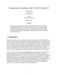
1
CEWES MSRC/PET TR/99-05
Coprocessing: Experience with CUMULVS and pV3
by
Randy Heiland
M. Pauline Baker
04h00399
Work funded by the DoD High Performance Computing
Modernization Program CEWES
Major Shared Resource Center through
Programming Environment andTraining (PET)
Supported by Contract Number: DAHC94-96-C0002
Nichols Research Corporation
Views, opinions and/or findings contained in this report are those of the author(s) and should not be construed as an official Department of Defense Position, policy, or decision unless so designated by other
official documentation.
Visualization & Virtual Environments at NCSA | Publications
Coprocessing: Experience with CUMULVS and pV3
Randy Heiland
and
M. Pauline Baker
NCSA
University of Illinois
January 1999
Abstract
Coprocessing involves running a visualization process concurrently with a simulation, and making intermediate
simulation results visible during the course of the run. Through computational monitoring, a researcher can watch the
progress of a run, perhaps ending the run if it looks unproductive. In this report, we experiment with applying two
software packages designed to support computational monitoring to a parallel version of a code for water quality
modeling.
1. Introduction
This report describes our early experience with software packages that address the problem of
interactive computation, or computational monitoring and steering (a.k.a., coprocessing). In an
earlier survey [1], we described scenarios where computational monitoring and steering could play
a valuable role in high performance computing (HPC). For example, a researcher might want to
visualize results of a running parallel simulation, rather than save data to disk and post-process -perhaps because the amount of data is simply too large. Monitoring a running simulation in this
fashion may in turn lead the researcher to stop the computation if it has gone awry, or to change
computational parameters and steer the computation in a new direction.
In the next section, we briefly survey existing packages for coprocessing. We explain why we
chose two packages, pV3 from MIT and CUMULVS from ORNL, for the focus of this
preliminary study. In Section 3, we briefly discuss PVM, since it is the common denominator of
both pV3 and CUMULVS. In Sections 4 and 5, we describe in some detail how each of these
packages operate and how an application developer would interface with each. An example
application, a parallelized water quality model of the Chesapeake Bay, is described in Section 6.
We connected this application to both pV3 and CUMULVS, as well as to a collaborative
visualization tool. This work was demonstrated at Supercomputing ’98 and is discussed in Section
7. Lastly, we provide a Summary and a list of References.
2. Coprocessing Survey
In an earlier survey, we considered a handful of packages that can provide partial solutions for the
challenge of computational monitoring and steering. We review those packages here and explain
why we focused our attention on two of them for this phase of the project. The packages
considered were the following:
Freely available
Restricted availability
CUMULVS
IBM Data Explorer
DICE
AVS
FASTexpeditions
SCIRun
pV3
Vis5D
VisAD
scivis
Given the obvious constraints of limited time and resources, a process of elimination was required
to select candidate packages for our initial study. Some simple criteria included:
Accessibility:
Is it downloadable (for free)?
Source code:
Is it available?
Stability:
Has the package been around awhile?
Is it used? Is it supported?
Dependencies: Does it depend on other packages?
Familiarity:
Do we have any experience with it?
What’s the learning curve like?
These criteria were merely guidelines, since there are usually trade-offs involved when choosing
software packages of any kind. For example a full-featured package may be difficult to install
and/or may have a steep learning curve. A very stable package may not be taking advantage of the
latest software language features. And you often get what you pay for -- free software usually
comes with no support.
From this collection of packages, CUMULVS, DICE from the Army Research Lab, and pV3 are
most appropriate for this study, since they appear to offer the most potential for immediate use
among researchers. Other candidates were judged as less appropriate for the current study for a
variety of reasons. The two Java-based packages were put aside as being too immature for
immediate use. In conversations with the lead author of one of these, Scivis from NPAC, we
learned that this package is undergoing major revision. The other Java-based package, VisAD
from University of Wisconsin, is also at an early stage in its life cycle. The author admits that the
package is appropriate for only small and medium-sized data sets -- i.e., it is not up to dealing with
big data. Further, VisAD relies not only on Java but on Java3D, which is currently available on
Sun and Windows only. While VisAD is not yet ready for transfer to the full research community,
it does offer real promise for the future. The development team has experience with developing
large-scale software -- Vis5D is in wide use. They are taking a broad-based approach to VisAD,
intending to handle unstructured as well as structured data, and intending to support collaborative
visualization as well.
FASTexpeditions from NASA Ames was less appealing since it is uses SGI’s proprietary GL
graphics library, rather than the newer industry standard, OpenGL. There are no plans to update to
OpenGL. After discussions with many researchers doing parallel visualization, AVS and IBM
Data Explorer were rejected for this study. Their greater strength is in the more traditional
approach, where visualization is done as a post-processing activity.
Of the three packages that offer promise for immediate use by computational researchers, DICE is
perhaps the most complete, even including GUI interfaces to selected codes. To date, DICE has
been used as a prototype vehicle to pioneer and showcase coprocessing with particular
applications. Deployment to a wide user community has not been a focus for the DICE project,
although the code is documented and available for download by contacting the project lead. We
found the installation process to be somewhat painful. DICE depends on some software patches
that had not yet been installed on our workstation. This demonstrates that DICE has not been fully
tested with a large user community. Nevertheless the DICE team was extremely helpful and we
eventually got it installed and running. The supplied examples ran fine and the documentation
appeared to be adequate to allow us to instrument a code for DICE. We did not include DICE in
this phase of our study due to time limitations, but we anticipate that we will work with DICE at a
later time.
CUMULVS and pV3 are of very different designs. pV3 is designed to outfit an existing [parallel]
client application with user-supplied routines for extracting various geometries. These are then
sent to and displayed by the pV3 front-end graphics server. CUMULVS, on the other hand, is
primarily designed to provide easy access to data being generated by a parallel application.
CUMULVS can supply an attached viewer with as much (or as little) of the computed data as
possible; pV3 does not. pV3 is specifically designed for CFD applications. CUMULVS on the
other hand is intended to be more general-purpose.
3. PVM
One similarity between pV3 and CUMULVS is that they both use PVM for their communication
layer. PVM provides the ability to dynamically attach and detach the visualization engine (the
’server’ in pV3 and the ’viewer’ in CUMULVS) from a running application.
The PVM (Parallel Virtual Machine) package is used by both pV3 and CUMULVS for
communication and for dynamic process attachment. For this project, we used version 3.4.beta7
(available for download from Netlib). An excellent reference for getting started using PVM can be
found at the Netlib page www.netlib.org/pvm3/book/node1.html. This walks a user through the
basic steps of installing PVM, running the PVM console, building a virtual machine, and spawning
processes.
One caveat is worth mentioning for environments using the Kerberos distributed authentication
service (for security purposes) -- as was the case for us at NCSA and for our demonstration at the
Supercomputing conference. After downloading the PVM package, the /conf subdirectory
contains various configuration options for all the supported architectures. One of these options is
the location of rsh (PVM uses the remote shell process). For our platform-dependent file,
SGI64.def, the DRSHCOMMAND was defined to use the standard /usr/bsd/rsh. However, in a
Kerberos environment, this had to be changed to invoke the Kerberos version of rsh (e.g.,
/usr/local/krb5/bin/rsh). After making this minor change, one can then build and install PVM.
4. pV3
pV3 (parallel Visual3) was developed at MIT and is targeted primarily for CFD codes. It is a
client-server system. The client (a researcher’s parallel application) must be augmented with
appropriate pV3 routines to extract geometry for graphics and to handle communication of
steering parameters, both of which are communicated to and from the pV3 server. The server is
embodied as a front-end graphical user interface (GUI). Some screen shots of the GUI are shown
in Figures 1 and 2. An adequate User’s Manual is provided for the server. This explains how to
dynamically select isovalues for isosurfaces, modify colormaps, display cutting planes, and much
more. Similarly, a Programmer’s Guide is provided for the client side. This describes the format of
the required user-supplied routines, the allowed topologies for grid cells, and more.
Figure 1. The pV3 server GUI with a sample client’s data.
Figure 2. With domain surfaces turned off, the pV3 server showing a density isosurface.
Unfortunately, the source code for pV3 is not available. Except for some client application code
examples, the rest of the package is binary format only. There are servers available for SGI, Sun,
DEC, and IBM workstations. There are no servers available for PC platforms. In addition to these
four platforms, the client-side pV3 library is also available for Cray and HP.
All example clients provided with the pV3 package deal with a single block computational grid,
sometimes displayed as an irregular physical grid. The process of displaying results from an
unstructured (computational) grid was not obvious. We were eventually successful at displaying
unstructured data, but only after some trial and error. The main confusion involved the notion of
pV3 ‘‘domain surfaces’’. For a single block of gridded data, the domain surfaces are trivially
defined as the outer faces of the cells. However, when one has unstructured data (cells), you must
explicitly tell pV3 which faces comprise the outer domain surface. Failure to do so leads to rather
obscure error messages.
One of the example clients provided with the pV3 package demonstrated a multi-client case. In
this simple example, the user types in a ‘‘processor identifier’’ (1,2,3,...). Therefore, by running
the client from two different windows and supplying different (sequential) IDs, it’s possible to
simulate a running parallel client application. In this example, the client program simply uses the
processor ID to offset the base geometry, resulting in replicated graphics in the server.
As a final note, the pV3 home page makes mention of pV3-Gold but the associated hyperlinks are
dead. pV3-Gold, a version with a nice Motif user interface, is not available at this time. It may
eventually become a commercial product. An image showing the pV3-Gold interface can be found
at sop.geo.umn.edu/~reudi/pv3b.html
.
5. CUMULVS
CUMULVS (Collaborative User Migration User Library for Visualization and Steering) was
developed at ORNL and is described as an ‘‘infrastructure library that allows multiple, possibly
remote, scientists to monitor and coordinate control over a parallel simulation program’’.
In practice, an application program is augmented with a few calls to routines in the CUMULVS
library. These routines describe the data distribution, the steerable parameters, and enable the
visualization. From a separate CUMULVS-aware ‘‘viewer’’ program, one requests blocks or
subsampled regions of data to visualize. The CUMULVS package does not provide a
self-contained 3D graphics viewer program (like the pV3 server). It does provide an AVS5 module
for connecting to a user-constructed AVS network (see Fig. 3). It also provides a couple of Tcl/Tk
viewers for viewing 2D representations such as slices (see Fig. 4), as well as a simple text viewer
which is especially useful for debugging. More importantly, CUMULVS can connect to any
user-constructed CUMULVS-aware viewer.
Figure 3. CUMULVS supplies an AVS5 module for connecting to AVS networks.
Figure 4. CUMULVS can connect to simple Tcl/Tk viewers for viewing 2D representations.
From a viewer, one makes requests to a running application for a ‘‘frame’’ of data and specifies
the frequency with which to receive frames. A frame of data is defined by a range and step size for
each coordinate index of the computational domain. In this regard, we see that CUMULVS, much
like pV3, is ideally suited for regularly gridded, block domain applications. CUMULVS, like pV3,
allows the nice feature of being able to dynamically attach/detach a viewer to/from a running
application (as mentioned in the above PVM Section).
CUMULVS is free to download with complete source and adequate documentation. One request
for the CUMULVS team is to augment the collection of PVM-based examples with at least one
MPI-based example application. This would prevent the confusion that we experienced when we
passed incorrect processor IDs to CUMULVS routines -- an example of which is shown in the next
section.
6. Monitoring Parallel CE-QUAL-ICM
The application currently being used to test these coprocessing packages is known as
CE-QUAL-ICM [2]. It was developed by Carl Cerco and Thomas Cole at the U.S. Army Corps of
Engineers Waterways Experiment Station (CEWES). It is a three-dimensional, time-variable
eutrophication model that has been used extensively to study the Chesapeake Bay estuary.
[Eutrophication is the process by which a body of water becomes enriched in dissolved nutrients
(as phosphates) that stimulate the growth of aquatic plant life, usually resulting in the depletion of
dissolved oxygen]. There have been varying sizes of grids used for the Chesapeake Bay model.
For our study, we use the largest grid available, consisting of approximately 10,000 hexahedral
cells. A top-down view of physical grid is shown in Fig. 5 and a view of the computational grid is
shown in Fig. 6. A 3D view of the cells in computational space is shown in Fig. 7.
Figure 5. Chesapeake Bay physical grid viewed from the top.
Figure 6. Chesapeake Bay computational grid viewed from the top.
Figure 7. Chesapeake Bay computational domain.
This application was parallelized by Mary Wheeler’s group [3] at the Center for Subsurface
Modeling (CSM), part of the Texas Institute for Computational and Applied Mathematics
(TICAM) at the University of Texas at Austin. They used MPI to perform the parallelization.
Executing on 32 processors vs. 1 processor, parallel CE-QUAL-ICM (or PCE-QUAL-ICM) runs
15 times faster than CE-QUAL-ICM. This surpasses the team’s goal of a 10-times speedup.
To understand the approach taken for the parallelization effort, it helps to understand how file-I/O
intensive the application is. Because CE-QUAL-ICM does not compute hydrodynamics, this
information must be read in at start-up. This (binary) file alone is nearly 900M in size. And this is
just one of dozens of input files. (The hydrodynamics file is the largest; the remaining files have a
total size of around 200M). The approach taken by the TICAM group was in three-phases:
run a pre-processor that would partition the input files across subdirectories (hence, the
pre-processor would only need to be run when configuring the parallel application for a
different number of processors)
run the (MPI) parallel CE-QUAL-ICM application (which needs to have parameters set and
then recompiled based upon the pre-processor results)
run a post-processor which locates the (local) output files spread across all subdirectories
(corresponding to all processors) and merges them into (global) output files which can then
be post-processed and/or archived.
CE-QUAL-ICM directly computes the following 24 fields (other fields are post-computed using
combinations of these together with other information):
1.
2.
3.
4.
5.
6.
7.
8.
9.
10.
11.
12.
13.
14.
15.
16.
17.
18.
19.
20.
21.
22.
23.
24.
Dissolved_silica
Particulate_silica
Dissolved_oxygen
COD
Refractory _particulate_P
Labile_particulate_P
Dissolved_organic_P
Total_phosphate
Refractory_particulate_N
Labile_particulate_N
Dissolved_organic_N
Nitrate-nitrite
Ammonium
Refractory_particulate_C
Labile_particulate _C
Dissolved_organic_C
Zooplankton _Group_2
Zooplankton _Group_1
Algal_Group_3
Algal_Group_2
Algal_Group_1
Inorganic_Solids
Salinity
Temperature
6.1 pV3
Figures 8 through 13 illustrate some results using pV3 on the CE-QUAL-ICM application.
Unfortunately, we are not yet able to run pV3 with the parallel application, due to the problem
discussed earlier for unstructured grids. To reiterate, the pV3 client requires that domain surface(s)
be supplied. If they are not defined or if they are defined incorrectly (pV3 does some internal
checks), then the client will generate errors and will not execute. It is a straightforward matter to
define the domain surface of the global Chesapeake Bay grid. However, when we decompose the
domain for parallel processing, the resulting multiple domain surfaces are not so easily obtained.
We have not yet solved this problem and consequently, can’t run this problem in parallel. We have
been in contact with Bob Haimes, the lead author for pV3, and are hopeful that we can arrive at a
solution in the near future. Until then, it is enlightening to see the visualizations that pV3 is
capable of producing and we continue to gain familiarity with using both the pV3 client library
and server.
Figure 8. Displaying temperature using slices.
Figure 9. Displaying the domain surfaces for salinity.
Figure 10. With pV3, the user can interactively change the display technique.
Figure 11. 3D contour lines mapped on a domain surface.
Figure 12. 3D contour lines.
Figure 13. An isosurface embedded within a translucent domain surface.
6.2 CUMULVS
CUMULVS ended up being our coprocessing package of choice. CUMULVS offers a simple and
clean design, full source code, and the flexibility of being able to attach custom viewers. The user
is free to use as simple or as complex a viewer as desired. Via CUMULVS, we connected
CE-QUAL-ICM to two viewers. In one case, we used a simple viewer based on the Visualization
ToolKit (VTK) [4]. This viewer allowed us to look at CE-QUAL-ICM’s output in many different
ways, including slices, isosurfaces, streamlines, etc. We could have made the viewer as complete
as VTK itself. We also connected CE-QUAL-ICM to the NCSA Collaborative Data Analysis
Toolsuite (CDAT) to support collaborative computational monitoring.
One of the first tasks undertaken with CUMULVS was to visualize the domain decomposition for
the parallel CE-QUAL-ICM. Fig. 14 shows the top-down view of the problem domain for
decompositions on 2, 4, 8, and 16 processors. We found the visual display of the decomposition to
be a valuable debugging aid. We were puzzled by the disconnected character of the decomposition
but confirmed with TICAM that it is correct. As illustrated in Fig. 15, the decomposition algorithm
assigns all sub-surface cells in a (depth) column to the same processor containing the surface cell.
Figure 14. Top-down view of domain decompositions for 2,4,8, and 16 processors.
Figure 15. A tilted view of the domain decomposition for two processors.
As mentioned in an earlier section, one problem we encountered during development was due to a
processor ID mismatch between CUMULVS, PVM, and MPI (Fig. 16). (We remind the reader that
PCE-QUAL-ICM had been parallelized using MPI.) Due to the manner in which local cells on
each processor were being mapped to global cells, the solution was not as trivial as one might
expect. Being able to visualize the results was a very valuable aid in the debugging process.
Figure 16. A processor ID mismatch problem yielded the incorrect results shown on the left. The
correct results are shown on the right.
7. Collaborative Computational Monitoring
Taking advantage of CUMULVS’ viewer flexibility, we also connected CE-QUAL-ICM to
CDAT. CDAT is a collection of cooperating applications running on various platforms. It supports
collaborative data analysis among users working at ImmersaDesks, Unix workstations, PC
workstations, and Web-browser only machines. While various configurations are possible, CDAT
currently makes use of VTK for visualization algorithms on the ImmersaDesk and workstations. It
utilizes Tango from NPAC to assist with registering participants and to provide whiteboards and
chat windows (Fig. 17). CDAT also uses an http server embedded in a workstation application to
push screen captures out to Web-only laptop.
Figure 17. CE-QUAL-ICM and CDAT.
We demonstrated this capability to attendees at Supercomputing ’98. At the NCSA Alliance booth,
we typically ran the application on four (SGI) processors and were still able to maintain interactive
updates of the visualization. At the DoD HPC booth, we ran the application on the 12-processor
SGI Origin. CDAT made it possible to collaboratively visualize results on the ImmersaDesk, a
desktop graphics workstation, and a Web-only PC.
The demonstration was the result of a lot of teamwork spread across several groups throughout the
country, including CEWES, TICAM, NCSA, and NPAC. Also, the ORNL developers (for
CUMULVS and PVM) and the VTK developers provided a substrate on which to do this work.
The demonstrations at Supercomputing ’98 went quite well and were attended by some very
appreciative scientists and software developers.
8. Summary
To date, we have surveyed and summarized the various packages available for coprocessing. In
this report, we outline the experience gained in applying two of these packages to a particular
application. In the next phase of this study, we will continue working with other coprocessing
packages, as well as resolve the problem encountered with pV3 in this phase. Also, while the
mechanism for performing computational steering has been readily available to us, we have not
yet exploited it in a truly beneficial manner. We need more feedback from application scientists
regarding this capability.
One could arguably claim that the parallel CE-QUAL-ICM used in this study does not constitute a
HPC application -- with only 10,000 cells of data to display. As this project evolves, we plan to
target other parallel applications with much larger datasets to visualize. HPC applications of the
near future will routinely involve thousands of processors and terabytes of data. It remains to be
seen whether today’s coprocessing systems will be able to function properly in such a setting.
We welcome comments and corrections from readers.
References
[1] Heiland, R., and M. P. Baker, ‘‘A Survey of Coprocessing Systems’’, CEWES MSRC PET
Technical Report 98-52, Vicksburg, MS, August 1998.
[2] Cerco, C., and Cole, T., ‘‘Three-dimensional eutrophication model of Chesapeake Bay’’, Tech
Report EL-94-4, U.S. Army Engineer Waterways Experiment Station, Vicksburg, MS, 1994.
[3] Chippada, C., Dawson, C., Parr, V.J., Wheeler, M.F., Cerco, C., Bunch, B., and Noel, M.,
‘‘PCE-QUAL-ICM: A Parallel Water Quality Model Based on CE-QUAL-ICM’’, CEWES MSRC
PET Technical Report 98-10, Vicksburg, MS, March 1998.
[4] Visualization ToolKit, http://www.kitware.com