1
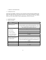
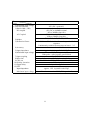
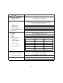
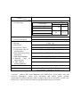
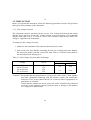
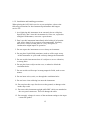
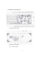
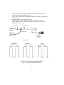
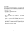
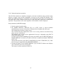
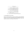
Oscilloscope
Analog Oscilloscope
Operation Manual
Oscilloscope
Analog Oscilloscope
Operation Manual
Safety Summary
Safety Precautions
Please take a moment to review these safety precautions.
They are provided for your protection and to prevent damage
to the oscilloscope.
This safety information applies to all operator and service
personnel.
Caution and warning statements.
CAUTION :
Is used
to indicate correct operating or maintenance
procedures in order to prevent damage to or destruction of the
equipment or other property.
WARNING : Calls attention to a potential danger that requires correct
procedures or practices in order to prevent personal injury.
Symbols
Caution(refer to accompanying documents) and Warning
Protective ground(earth) symbol
5
Introduction
Thank you for purchasing a EZ product. Electronic measuring instruments
produced by EZ digital are high technology products made under strict quality
control. We guarantee their exceptional and utmost reliability. For proper use of
the product please read this manual carefully.
Instructions
1. To maintain the precision and reliability of the product use it in the
standard conditions(temperature 10℃~35℃ and humidity 45%~85%)
2. After turning on power, please allow a 15minute preheating warmup period
before using.
3. Triple-line power cord is to be used for this product. But when you are
using doubleline power cord. Make sure for safety
4. For quality improvement the exterior design and specifications of the
product can be changed without prior notice.
5. If you have further questions concerning use, please contact the EZ
Digital service center or sales outlet.
6
Warranty
Warranty service covers a period of one year from the date of original purchase.
In case of technical failure within a year, repair service will be provided by our
service center or sales outlet free of charge.
We charge for repairs after the one-year warranty period expires.
When the failure is a result of user=s neglect, natural disaster or accident, we
charge for repairs regardless of the warranty period.
For more professional repair service, be sure to contact our service center or
sales outlet.
7
CONTENTS
1.PRODUCT DESCRIPTIONS
-------------------
10
1-1. INTRODUCTION --------------------------------------------- 10
1-2. SPECIFICATIONS ------------------------------------------- 10
1-3. PRECAUTIONS ---------------------------------------------- 10
1-4. ACCESSORY ------------------------------------------------ 12
2. OPERATING INSTRUCTIONS
----------------
2-1. FUNCTION of CONTROLS,
CONNECTORS, AND INDICATORS -------------------2-1-1. Display and Power Blocks ---------------------------2-1-2. Vertical Amplifier Block -------------------------------2-1-3. Sweep and Trigger Blocks ---------------------------2-1-4. Miscellaneous Features ------------------------------2-2. BASIC OPERATING PROCEDURES ------------------2-2-1. Signal Connections ------------------------------------2-2-2. Preliminary Control Settings and Adjustments --2-2-3. Probe adjustment ---------------------------------------2-2-4. Signal -trace Operation --------------------------------2-2-5. Multi-trace Operation -----------------------------------2-2-6. Trigger Options ------------------------------------------2-2-7. Additive and Differential Operation -----------------2-2-8. X-Y Operation --------------------------------------------2-2-9. Delayed-time base Operation ------------------------2-3. MEASUREMENT APPLICATIONS ----------------------2-3-1. Amplitude Measurements -----------------------------2-3-2. Time Interval Measurements -------------------------2-3-3. Frequency Measurement ------------------------------2-3-4. Phase Difference Measurement ---------------------2-3-5. Rise Time Measurement --------------------------------
8
17
18
18
18
20
23
23
23
25
26
28
29
30
35
36
37
38
39
43
46
46
50
3. USER MAINTENANCE GUIDE ----------------
53
3-1. CLEANING ------------------------------------------------------- 53
3-2. CALIBRATION INTERVAL ----------------------------------- 53
4. DIAGRAMS
------------------------------------------
54
4-1. EXTERNAL VIEWS -------------------------------------------- 54
4-2. BLOCK DIAGRAM --------------------------------------------- 55
9
1. PRODUCT DESCRIPTIONS
1-1. INTRODUCTION
OS-5100 is the 100MHz, 2 channels, 2 traces which has excellent functions including wide
band width, high sensitivity, two timebase generator, delay sweep and divided TV trigger
Signal, It reduces the measurement error, and uses 6” squared type CRT with internal
fluorescent scale which enables to take the photograph of observed waveform.
1-2. SPECIFICATIONS
1-3. PRECAUTIONS
MODEL
OS-5100
SPEC
* CRT
1) Configuration
2) Accelerating potential
6-inch rectangular screen with internal graticule : 8 X 10
div (1div=1cm), marking for measurement of rise time,
2mm subdivisions along the central axis.
+ 9kV approx. (ref. Cathode)
3) Phosphor
P31 (standard)
4) Focussing
Possible (with autofocus correction circuit)
5) Trace rotation
Provided
6) Scale Illumination
Variable
7) Intensity control
Provided
* Z-Axis input
(Intensity Modulation)
1) Input signal
2) Band-width
Positive going signal decreases intensity +3Vp-p or more
signal cases noticeable modulation at normal intensity
setting
DC ~ 3.5MHz (-3dB)
DC
3) Coupling
4) Input impedance
17 ~ 22㏀
10
MODEL
OS-5100
SPEC
5) Maximum input voltage
* Vertical Deflection
1) Band-width (-3dB)
DC coupled
AC Coupled
2) Modes
3) Deflection Factor
4) Accuracy
5) Input impedance
6) Maximum input voltage
7) Input coupling
8) Rise time
9) CH1 out
10) Polarity invertion
11) Signal delay
12) EXT
Input Impedance
Maximum input voltage
20V (DC + peak AC)
(X1) DC to 100MHz normal
DC to 20MHz (2mv/div)
(X1) 10Hz to 100MHz normal
10Hz to 20MHz (2mv/div)
CH1, CH2, ALT, CHOP, ADD
2mV/div to 5V/div in 11 calibrated steps of a 1-2-5
sequence
Continuously variable between steps at least 1 : 2.5
normal : ±3%
Approx. 1 ㎖ in parallel with 25pF
Direct : 250V (DC + peak AC),
With probe : refer to probe specification
AC – DC, GND
3.5ns or less (17.5ns or less : 2mV/div)
20mV/div into 50Ω : 50Hz to 30MHz (-3dB)
CH2 only
delay cable supplied
approx. 1 ㏁ in parallel with 22pF
Direction connection 250V (DC + peak AC)
11
MODEL
OS-5100
SPEC
* Horizontal deflection
1) Display modes
2) Time base A
Hold-off time
3) Time base B
Delayed sweep
4) Sweep magnification
5) Accuracy
* Trigger system
1) Modes
2) Source
3) Slope
4) Sensitivity and
Frequency
AUTO, NORM
TV-V, TV-H
5) ALT TRIGGER
* X-Y operation
1) Frequency bandwidth
2) X-Y phase difference
* Calibrator (probe adjustor)
A, A INT, B, X-Y, B TRIG’
01㎲/div to 0.5s/div in 21 calibrated steps,
1-2-5 sequence, uncalibrated continuous control
between steps at least 1:2.5
Variable with the holdoff control
0.1㎲/div to 10㎲/div in calibrated steps 1-2-5 sequence
1 div or less 10 div or more
10 times (maximum sweep rate : 10ns/div
±3%, ±5% (X 10)
AUTO, NORM, TV-V, TV-H
INT, LINE, EXT
+ or Freq.
Internal
External
30Hz~10MHz
0.48 div
200mV
10MHz~100MHz
1.5 div
600mV
TV-V, TV-H
1.0 div
0.2V
30Hz~10MHz
1.5 div
-
10Hz~100MHz
3.0 div
-
Dc coupling : DC ~ 2MHz
AC coupling : 10Hz ~ 2MHz
Within 3° (up to 100kHz at DC)
Approx. 1kHz frequency, 0.5V(±3%) square wave
Wave duty ratio : 50%
12
Model
OS-5100
SPEC
* Power Supply I
1) Voltage range
Voltage range
Fuse (250V)
UL198G
1EC127
100V ( 90~110V) / AC
2A
120V (108~132V) / AC
F2A
220V (197~242V) / AC
230V (207~250V) / AC
2) Frequency
3) Power consumption
* Physical Charac.
1) Weight
2) Dimension
* Environmental Charac.
1) Temperature range for
rated operation
2) Max. ambient operating
temperature
3) Max. storage temperature
4) Humidity range for
rated operation
5) Max. ambient
operating humidity
* Safety
* EMC
1A
F1A
50 / 60 HZ
approx. 60W
8.5kg±1kg
320m(W) X 140mm(H) X 430mm(L)
+10℃ to +35℃ (+50℉ to +95℉)
0℃ to +40℃ (+32℉ to +104℉)
-20℃ to +70℃ (-4℉ to +158℉)
45% to 85% RH
35 % to 85% RH
EN61010-1 overvoltage CAT II, degree of pollution 2
Interference : EN50081-1
Susceptability : EN50082-1, IEC801-2,3,4
<Caution> : Sources like small hand-held radio transceivers, fixed station radio and
television transmitters, vehicle radio transmitters and cellular phones generate
electromagnetic radiation that may induce voltage in the leads of a test probe. In such cases
the accuracy of the oscilloscope cannot be guaranteed due to physical reasons.
13
1-3. PRECAUTION
Before you operate this instrument, follow the following procedure to ensure safe operation
and to prevent any damage to the instrument.
1-3-1. Line voltage selection
This instrument must be operated with the correct. Line Voltage Selection switch setting
and the correct line fuse for the line voltage selected to prevent damage. The instrument
operates from either a 90 to 132 volts or a 198 to 250 volts line voltage source. Before line
voltage is a applied to the instruments.
To change the line voltage selection :
1. Make sure the instrument is disconnected from the power source.
2. Pull out the Line Fuse Holder containing the fuse for overload protection. Replace
the fuse in the holder with the correct fuse from Table 1-1 slide the arrow mark to
the desired position and plug it in.
Table 1-1 Line Voltage Selection and Fuse Ratings
Voltage
Arrow
90 to 110volts
108 to 132volts
198 to 242volts
207 to 250volts
100
120
220
230
Fuse (250V)
UL198G
IEC127
2A
F2A
1A
F1A
<Caution> This product has the ground chassis (3 wire power cord is used). Check whether
any other equipment connecting with this product requires the transformer
before use. If so, do not connect the DC/AC or the hot chassis equipment if no
transformer is available.
Do not directly connect it to the AC power nor to the circuit directly connected
to the AC power. Otherwise serious personal injury or damage to this product
for a long time without trouble.
14
1-3-2. Installation and handling precautions
When placing the OS-5100 in service at your workplace, observe the
following precautions for best instrument performance and longest
service life.
1. Avoid placing this instrument in an extremely hot or cold place.
Specifically, don’t leave this instrument in a close car, exposed to
sunlight in midsummer, or next to a space heater.
2. Don’t use this instrument immediately after brining it in from the
cold. Allow time for it to warm to room temperature. Similarly,
don’t move it from a warm place to a very cold place, as
condensation might impair its operation.
3. Do not expose the instrument to wet or dusty environments.
4. Do not place liquid-filled containers (such as coffee cups) on top
of this instrument. A spill could seriously damage the instrument.
5. Do not use this instrument where it is subject to servere vibration,
or strong blow.
6. Do not place heave object on the case, or otherwise block the
ventilation holes.
7. Do not use this oscilloscope in strong magnetic fields, such as near
motors.
8. Do not insert wires, tools, etc. through the ventilation holes.
9. Do not leave a hot soldering iron near the instrument.
10. Do not place this scope face down on the ground, or damage to the
knobs may result.
11. Do not use this instrument upright while BNC cables are attached to
the rear-panel connectors. This will damage the cable.
12. Do not apply voltages in excess of the maximum ratings to the input
connectors probes.
15
1-1. ACCESSORY
The following accessories are included in the packing of this product :
(1) Operating manual : 1copy
(2) AC power code : 1EA
(3) Probe (Option : 2 EA
(4) Fuse : 1EA
16
2. OPERATING INSTURCTIONS
(a) FRONT-PANEL ITEMS
(b) REAR-PANEL ITEMS
Fig. 2-1. PANEL ITEMS
17
This section contains the information needed to operate the OS-5100 and
utilize it in a variety of basic and advanced measurement procedures.
Included are the identification and function of controls, connectors, and
indicators, startup procedures, basic operating routines, and selected
measurement procedures.
2-1. FUNCTION OF CONTROLS, CONNECTORS, AND INDICATORS
Before turning this instrument on, familiarize yourself with the controls,
connectors, indicators, and other features described in this section.
The following descriptions are keyed to the items called out in Figures 2-1.
2-1-1. Display and power blocks
[1] POWER SWITCH
: Push in to turn instrument power on and off.
[2] POWER LAMP
: Green lights when power is on
[3] INTENSITY
: Adjust the brightness of the CRT display. Clockwise
rotation increases brightness.
[4] FOCUS
: To obtain maximum trace sharpness
[5] TRACE ROTATION
: Allows screwdriver adjustment of trace alignment with
regard to the horizontal graticule lines of the CRT
[6] SCALE ILLUM
: To adjust graticule illumination for photographing the
CRT display
[7] VOLTAGE SELECTOR
: Permits changing the operating voltage range
[8] POWER CONNECTOR
: Permits removal or replacement of the AC power cord
2-1-2. Vertical amplifier block
[9] CH1 X IN connector
: For applying an input signal to vertical amplifier channel
1, or to the X-axis (horizontal) amplifier during X-Y
operation
<CAUCTION> To avoid damage to the oscilloscope, do not apply more than 250V (DC +
Peak AC) between “CH1” terminal and ground
18
[10] CH2 or Y IN connector
: For applying an input signal to vertical
amplifier channel 2, or to the Y-axis
(vertical) amplifier during X-Y operation
<CAUCTION> To avoid damage to the oscilloscope, do not apply more than
250V (DC + Peak AC) between “CH2” terminal and ground
[11] [12] AC-DC, GND
: To select the method of coupling the input signal to the
CH1, CH2 vertical amplifier.
AC : AC position inserts a capacitor between the input
connector and amplifier to block any DC component in
the input signal
DC : DC position connects the amplifier directly to its input
connector, thus passing all signal components on to the
amplifier.
GND : GND position connects the amplifier to ground instead
of the input connector, so a ground reference can be
established
[13] [14] VOLTS/ div
: To select the calibrated deflection factor of the input
signal fed to the CH1, CH2 vertical amplifier.
[15] [16] VARIABLE
: Provide continuously variable adjustment of deflection
factor between steps of the VOLTS/DIV switches,
VOLTS/DIV calibrations are accurate only when the
VARIABLE controls are click-stopped in their fully
clockwise position
[17] CH1 POSITION
: For vertically positioning the CH1 trace on the CRT
screen, Clockwise rotation moves the trace up,
counterclockwise rotation moves the trace down.
[18] CH2 POSITION
: It operates in the same manner as described in the step
(17). Pulling the knob out, the CH2 waveform is
reversed.
19
[19] V MODE
: To select the vertical-amplifier display mode.
CH1 : CH1 position displays only the channel 1 input signal
on the CRT screen.
CH2 : CH2 position displays only the channel 2 input signal
on the CRT screen.
ALT : The waveform appears alternatively at each sweep end.
This function is useful to measure at the speed faster
than 50㎲/div. Multi-phenomena or signal sweep
CHOP : Each waveform appears concurrently, and it is useful
to measure at the speed slower than 50㎲/div. Multiphenomena or signal sweep.
ADD : ADD position displays the algebraic sum of CH1 &
CH2 signals
[20] CH1 OUTPUT CONNECTOR : Provides amplified output of the channel 1 signal
suitable for driving a frequency counter or other
instrument
2-1-3. Sweep and trigger blocks
[21] HORIZONTAL DISPLAY : To select the sweep mode
A : A pushbutton sweeps appear on the scream at the main
(A) timebase rate when pressed.
A INT : A and B sweeps appears on the screen in turn. In this case
B sweeps appears on the emphasized part of A sweep. The
location of the emphasized part is decided by adjusting the
DLY’D POSITION.
A and B sweeps are displayed along the A and B
TIME/DIV Switches respectively. Simultaneously press A
and B buttons.
B : The modulated part of brightness is magnified and
displayed on the entire screen.
X-Y
: Enables to select the X-Y operation
20
B TRIG’D
: The delay seep is triggered by the first trigger pulse.
[22] A TIME/DIV
: To select either the calibrated sweep rate of the main (A)
timebase, the delay-time range or delayed-sweep operation
[23] B TIME/DIV
: To select the calibrated sweep rate of the delayed (B)
timebase
[24] DLY’SD POSITION
: To determine the exact starting point within the A timebase
delay range at which the B timebase will begin sweeping
[25] A VARIABLE
: Continuously changes the A sweep time to the calibrated
position.
PULL X 10MAG : Pulling switch extends the seep time ten times. In this case,
sweep time becomes one tenth the TIME/DIV value.
Pulling the X 10 MAG switch when the zone to be
magnified is aligned with the center scale of vertical axis
by adjusting the horizontal axis, the magnified waveform
appears in symmetry. In this case, sweep time becomes one
tenth the TIME/DIV value.
[26] HORIZONTAL POSITION : To adjust the horizontal position of the traces displayed
on CRT. Clockwise rotation moves the traces to the right,
counterclockwise rotation moves the traces to the left.
[27] FINE
[28] TRIGGER MODE
: It is used to make fine adjustment of horizontal position
: To select sweep triggering mode.
AUTO : AUTO position selects free-running sweep where a
baseline is displayed in the absence of a signal. This
condition automatically, reverts to triggered sweep when
a trigger signal of 25Hz or higher is received and other
trigger controls are properly set.
21
NORM : NORM position produces sweep only when a trigger
signal is received and other controls are properly set. No
trace is visible if any trigger requirement is missing.
This mode must be used when the signal frequency is
25Hz or lower.
TV-V : TV-V position is used for observing a composite video
signal at the frame rate.
TV-H : TV-H position is used for observing a composite video
signal at the line rate.
[29] TRIGGER SOURCE
: To conveniently select the trigger source.
INT : CH1 (CH2) position selects the channel 1 (channel 2)
signal as the trigger source.
LINE : LINE position selects a trigger derived from the AC
power line. This permits the scope to stabilize display
line-related components of a signal even if they are very
small compared to other components of the signal.
EXT : The signal applied to the input terminal of EXT is
used as trigger signal. When small internal signal or any
unexpected signal prevents the trigger, the outside
trigger signal source can be entered to stabilize the
measurement of waveform.
[30] HOLD OFF
: Allows trigger on certain complex signals by changing
the holdoff (dead) time of the main (A) sweep. This
avoids triggering on intermediate trigger points within
the repetition cycle of the desired display. The
holdofftime increase with clockwise rotation.
22
[31] TRIG LEVEL
: To select the trigger signal amplitude at which triggering
occurs. When rotated clockwise, the trigger point moves
toward the positive peak of the trigger signal. When this
control is rotated counterclockwise, the trigger point
moves toward the negative peak of the trigger signal.
TIGGER SLOPE : To select the positive or negative slope of the trigger
signal for initialing sweep. Pushed in, the switch selects
the positive (+) slope. When pulled, this switch selects
the negative (-) slope.
[32] EXT TRIG IN
: For applying external trigger signal to the trigger circuits.
<CAUTION> To avoid damage to the oscilloscope, do not apply more than 250V (DC +
peak, AC) between “EXT Trig In” terminal and ground.
2-1-4. Miscellaneous Features
Connector
[33] EXT BLANKING INPUT : For applying signal to intensity modulate the CRT. Trace
brightness is reduced with a positive signal, and
increased with a negative signal.
[34] PROBE ADJUST
: Outputs square wave (0.5V, P-P, 1KHz) to calibrate
probe and vertical amplifier.
[35] GROUND CONNECTOR
: Provides an attachment point for a separate ground
lead.
[36] VERT MODE
CH1
CH2
: Selects mode of operation for vertical amplifier system
: Channel 1 is displayed on the CRT
: Channel 2 is displayed on the CRT
2-2. BASIC OPERATING PROCEDURES
2-2-1. Signal Connections
There are three methods of connecting an oscilloscope to the signal you
with to observe. They are a simple wire lead, coaxial cable, and scope
probes.
23
1. A simple lead wire
2. Coaxial cable
3. Scope probes
1. A simple lead wire
A simple lead wire may be sufficient when the signal level is high and the source
impedance low (such as TTL circuitry), but is not often used. Unshielded wire picks up
hum and noise ; this distorts the observed signal when the signal level is low.
Also, there is the problem of making secure mechanical connection to the input connection
to the input connectors. A binding post-to BNC adapter is advisable in this case.
2. Coaxial cable
Coaxial cable is the most popular method of connecting an oscilloscope to signal sources
and equipment having output connectors. The outer conductor of the cable shields the
central signal conductor from hum and noise pickup. These cables are usually fitted with
BNC connectors on each end, and specialized cable and adaptors are readily available for
mating with other kind of connectors.
3. Scope probes
Scope probes are the most popular method of connecting the oscilloscope to circuitry.
These probes are available with 1 X attenuation (direct connection) and 10 X attenuation.
The 10 X attenuator probes increase the effective input impedance of the probe/scope
combination to 10 megohms shunted by a few picofarads. The reduction in input
capacitance is the most important reason for using attenuator probes at high frequencies,
where capacitance is the major factor in loading down a circuit and distorting the signal.
When 10 X attenuator probes are used, the scale factor (VOLTS DIV switch setting) must
be multiplied by ten.
Despite their high input impedance, scope probes do not pickup appreciable hum or noise.
As was the case with coaxial cable, the outer conductor of the probe cable shields the
central signal conductor. Scope probes are also quite convenient from a mechanical
standpoint.
To determine if a direct connection with shielded cable is permissible, you must know the
source impedance of the circuit you are connecting to, the highest frequencies involved,
and the capacitance of the cable. If any of these factors are unknown, use a 10 X low
capacitance probe.
24
2-2-2. Preliminary control settings and adjustments
Before placing the instrument in use, set up and check the instrument as follows ;
1. Set the following controls as indicated
Power source part
POWER SWITCH [1]
INTEN [3]
FOCUS [4]
: OFF (coming up)
: Fully counterclockwise
: Center
Vertical Part
AC-DC, GND [11, 12]
VOLT/DIV [13, 14]
VERTICAL POSITION [17, 18]
VARIABLE [15, 16]
V. MODE [19]
: AC
: 10Mv
: Locates at center while being pressed
: Fully clockwise while being pressed
: CH1
Horizontal part
TIME/DIV [22]
TIME VARIABLE [25]
HORIZONTAL POSITION [26]
FINE POSITION [27]
: 0.5ms
: Fully clockwise while being pressed
: Center
: Center
Trigger part
TRIGGER MODE [28]
TRIGGER SOURCE [29]
HOLD OFF [30]
TRIGGER LEVE [31]
SLOPE [31]
: AUTO
: INT
: NORM (Max. counterclockwise)
: Center
: + (pressed)
25
2. Connect the AC Power Cord to the Power Connector [8], then plug the cord into a
convenient AC outlet.
3. Press in the Power switch [1], The POWER lamp [2] should light immediately. About 30
seconds later, rotate the INTEN control clockwise until the trace appears on the CRT screen.
Adjust brightness to you liking.
< Note> A burn-resistant material is used in the CRT. However if the CRT is left with an
extremely bright dot or trace for a very long time, the screen may be damaged.
Therefore, if a measurement requires high brightness, be certain to turn down the
INTEN control immediately afterward. Also, get in the habit of turning the
brightness way down if the scope is left unattended for any period of time.
4. Turn the FOCUS control [4] for a sharp trace.
5. Turn the CH1 Vertical POSITION CONTROL [17] to move the CH1 trace to the center
horizontal graticule line.
6. Turn the Horizontal POSITION control [26] to align the left edge of the trace with the
left-most graticule line.
2-2-3. Probe adjustment
When applying the external signal to be measure using oscilloscope, use probe. The applied
waveform is displayed on the CRT of oscilloscope. This product has two points.
1 X (direct connection) and 10 X (attenuation). At 10 X point, the input impedance of
oscilloscope increases, which attenuates the input signal by 1/10. Therefore, it is necessary
to multiply 10 to the measurement unit (volts/div.)
The damping probe is used for high frequency measurement because of the reduction of
input capacity which distorts signal and reduces the load.
Using any incorrectly calibrated probe may cause error in the measurement. So adjust the
probe as follows :
26
1. Connect probe to CH1 X IN [9]. With CH1 input coupling set to DC,
connect tip to PROBE ADJUST [34].
In this case, set the probe damping position to 10 X and set VOLT/DIV
[13] to 10mV.
2. Adjust Trigger Level to stabilize screen.
When the top or a part of spherical wave is slanted or has any
tooth, adjust the probe adjustment trimmer as shown in Fig. 2-2(b)
using small screw driver.
Hook Cover
Main Body
X1
Retractable
Hook Tip
X10
Ground Cover
Capacitance
Correction
Trimmer
Ground Clip
(a) PROBE
CORRECTLY
COMPENSATED
UNDER
COMPENSATED
OVER
COMPENSATED
(b) EFFECTS OF PROBE COMPENSATION
Fig. 2-2. PROBE COMPENSATION
27
2-2-4. Single-trace operation
Single-trace operation with single timebase and internal triggering is the most elementary
mode of the OS-5100 Use this mode when you wish to observe only a single signal, and not
be disturbed by other traces on the CRT. Since this is fundamentally a two-channel
instrument, you have a choice for your single channel. Channel has an output terminal [20]
use channel 1 if you also want to measure frequency with a counter while observing the
waveform. Channel 2 has a INVERT [18] to convert the polarity.
CH1 Signal display
1. Set the initial screen as described in paragraph 1. 2-2-2.
2. Set the CH1 input coupling [11] to AC.
3. Connect the signal to CH1 connector [9].
<Note> Do not apply power voltage (DC + PEAK AC) higher than 250V.
4. Adjust CH1 VOLT/DIV switch [13] and vertical POSITION (17) terminal to place
the signal in the measurable area.
5. Adjust TRIGGER LEVEL [31] to display a stable waveform.
6. Adjust a TIME/DIV switch [22] and horizontal POSITION [26] to place the
waveform in the measurable area.
When it is difficult to measure high frequency signal with A TIME/DIV switch [22]
set to 10ns at these have to many cycle, pull VARIABLE [25] to pull X 10 MAG..
Then retry to measure.
7. When measuring any damped or distorted low frequency signal, set the vertical input
coupling to DC.
CH2 Signal display
Except for the following step, the method to display CH2 signal is same as that of CH1.
1. Set V MODE [19] switch to CH2,. And TRIGGER SOURCE switch [29] to INT.
28
2. Set CH2 input coupling [12] to AC, and connect signal to CH2 input connector.
3. Adjust CH2 VOLTS/DIV switch [14] and vertical position terminal [18] to place
signal in the measurable area.
TRIGGER signal display
When signal is applied to TRIGGER generator, signal is displayed on the CRT.
1. Set the initial screen as described in paragraph 1, 2-2-2.
2. Set CH1, CH2 input coupling [11] and [12] to AC.
3. Set V mode switch (19) to ALT or CHOP.
4. When TRIGGER SOURCE switch [29] is set to INT, the output from CH1 input
amplifier is displayed on CRT.
5. When TRIGGER SOURCE switch [29] is set to INT, the output from CH2 input
amplifier is displayed on CRT.
6. When TRIGGER SOURCE switch [29] is set EXT, the signal is fed to TRIGGER
generator and displayed on CRT.
2-2-5. Dual-trace operation
For dual-trace measurement, two waveforms out of CH1. CH2 may be displayed in ALT or
CHOP mode.
1. When selecting the desirous channel, the CH1 and CH2 bright line are selectively
displayed on the CRT.
2. Select the ALT for the related high frequency signal (sweep rate is higher than 50㎲
/div.)
3. Select the CHOP for the related low frequency signal (sweep rate is lower than 50㎲
/div.)
4. If signal with same frequency is displayed, set TRIGGER SOURCE switch [29] to
29
INT and the channel to which waveform with steeper slope is applied.
As for other signal, if the frequency is of multiple number, set TRIGGER SOURCE
switch [29] to the channel to which low frequency is applied.
Remember that no trigger is possible on the screen if the currently used channel is
not adjusted using TRIGGER SOURCE [29]
5. If non-synchronized signal with different frequency is displayed, please set
TRIGGER SOURCE SWITCH (29) to “INT” and set “Vert” of the INT SWITCH
(36).
Remember that vert trigger is possible on the screen only when VERTICAL MODE
SWITCH (19) is selected to “ALT”
2-2-6. Trigger options
Triggering is often the most difficult operation to perform on an oscilloscope because of the
many options available and the exacting requirements of certain signals.
(1) TRIGGER MODE [28] selection
AUTO, NORM TRIGGER MODE
When the NORM trigger mode is selected, the CRT beam is not swept horizontally across
the face of the CRT until a sample of the signal being observed, or another signal
harmonically related to it, triggers the timebase. However, this trigger mode is inconvenient
because no base line appears on the CRT screen in the absence of a signal, or if the trigger
controls are improperly set. Since an absence of trace can also be due to an improperly set
Vertical POSITION control or VOLTS/DIV switch, much time can wasted in determining
the cause. The AUTO trigger mode solves this problem by causing the timebase to
automatically free run when not triggered. This yields a single horizontal line with no
signal, and a vertically-deflected but non-synchronized display when vertical signal is
present but the trigger controls are improperly set This immediately indicates what is wrong.
The only hitch with AUTO operation is that signals below 25Hz cannot, and complex
signals of any frequency may not, reliably trigger the timebase. Therefore, the usual
practice is to leave the TRIGGER MODE switch [28] set to AUTO, but reset it to NORM if
any signal (particularly one below 25Hz) fails to produce a stable display.
30
TV-V, TV-H TRIGGER MODE
The TV-V and TV-H positions of the Trigger MODE switch insert a TV sync separator into
the trigger chain, so a clean trigger signal at either the vertical-or horizontal-repetition rates
can be removed from a composite video signal (Fig 2-3 (b)), set the TRIGGER MODE
switch to TV-V. To trigger the scope at the horizontal (line) rate (Fig 2-3(c)), set the
TRIGGER MODE switch to TV-H. For best results, the TV sync polarity should be
negative (Fig 2-3 (d)) when the sync separator is used.
31
32
(2) TRIGGER POINT selection
The SLOPE switch [31] determines whether the sweep will on a
positive-going or negative-going transition of the trigger signal.
The pressed position is the starting point of rise, and pulled
position is the starting point of drop.
Always select the steepest and most stable slope or edge. For
example, small changes in the amplitude of the sawtooth shown in
Fig 2-4 (a) will cause jittering if the timebase is triggered on the
positive (ramp) slope, but have no effect if triggering occurs on
the negative slope (a fast-fall edge).
In the example shown in Fig 2-4(b), both leading and trailing edges
are very steep (fast rise and fall times). However, triggering from
the jittering trailing edge will cause the entire trace to jitter,
making observation difficult. Triggering from the stable leading
edge (+ slope) yields a trace that has only the trailing-edge
jitter of the original signal. If you are ever in doubt, or have an
unsatisfactory display, try both slopes to find the best way.
The LEVEL control [31] determines the point on the selected slope
at which the main (A) timebase will be triggered. The effect of the
LEVEL control on the displayed trace is shown in Fig. 2-5. The +,
0, and-panel markings for this control refer to the waveform’s zero
crossing and points more positive (+) and more negative (-) than
this. If the trigger slope is very steep, as with square waves or
digital pulses, there will be no apparent change in the displayed
trace until the LEVEL control is rotated past the most positive or
most negative trigger point, whereupon the display will free run
(AUTO sweep mode) or disappear completely (NORM sweep mode),
trigger at the mid point of slow-rise waveforms (such as sine and
triangular waveforms), since these are usually the cleanest spots
on such waveforms.
33
34
2-2-7. Additive and differential operation
Additive and differential operation are forms two-channel operation where two signals are
combined to display one trace, In additive operation, the resultant trace represents the
algebraic sum of the CH1 and CH2 signals, In differential operation, the resultant trace
represents the algebraic difference between the CH1 and CH2 signals.
To set up the OS-5100 for additive operation, proceed as follows :
1. Set V MODE switch [19] to ALT or CHOP, display two channels.
2. Make sure both VOLTS/div switches [13] and [14] are set to the same position and
the VARIABLE control [15] and [16] are click-stopped fully clockwise. If the signal
levels are very different, set both VOLTS/div switches [13]. [14] to the position
producing a large on-screen display of the highest-amplitude signal.
3. Trigger from the channel having the biggest signal.
4. Set the V MODE switch ADD position. Then the single trace resulting is the
algebraic sum of the CH1 and CH2 signal. Either of both of the Vertical POSITION
controls [19] and [20] can be used to shift the resultant trace.
<Note> If the input signals are in-phase, the amplitude of the resultant trace will be the
arithmetic sum of the individual traces (eg., 4.2 div + 1.2 div = 5.4 div)
If the input signals are 180° out-of phase, the amplitude will be the difference
(eg., 4.2 div ~ 1.2 div = 3.0 div)
5. If the P-P amplitude of the resultant trace is very small, turn both VOLTS/div
switches [13], [14] to increase the display height. Make sure both are set to the same
position.
To set up the OS-5100 for differential operation do everything just described and also pull
the CH2 Vertical POSITION knob [20] to activate the PULL CH2 INV switch. The single
trace resulting is the algebraic difference of the CH1 and CH2 signals. Now if the input
signals are in-phase, the amplitude of the resultant trace is the arithmetic difference of the
individual traces (eg., 4.2 div~1.2 div = 3.0 div.) If the input signals are 180° out-of-phase,
the amplitude of the resultant trace is the arithmetic sum of the individual traces (eg., 4.2
div + 1.2 div = 5.4 div).
35
2-2-8. X-Y operation
The internal timebase of the OS-5100 are not utilized in X-Y operation; deflection in both
the vertical and horizontal directions is via external signals. Vertical channel I serves as the
X-axis (horizontal) signal processor, so horizontal and vertical axis have identical control
facilities.
All of the V mode, and trigger switches, as well as their associated controls and connectors,
are inoperative in the X-Y mode.
To set up OS-5100 for X-Y operation, proceed as follows :
1. Push the X-Y switch [21]
<Caution> Reduce the trace intensity, lest the undeflected spot damage the CRT
phosphor.
2. Apply the vertical signal to the CH2 or Y IN connector [10], and the horizontal
signal to the CH1 or X IN connector [9]. Once the trace is deflected, restore normal
brightness.
3. Adjust the trace height with the CH2 VOLTS/DIV switch [14], and the trace width
with the CH1 VOLTS/DIV SWITCH [13]. The VARIABLE controls can be used if
greater is necessary, so leave the TIME VARIABLE control [25] knob pushed in.
4. Adjust the trace position vertically (Y axis) with the CH2 Vertical POSITION
control [18]. Adjust the trace position horizontally (X axis) with the Horizontal
POSITION control [26] ; the CH1 Vertical POSITION control has no effect during
X-Y operation.
5. The vertical (Y axis) signal can be inverted by pulling the CH2 Vertical POSITION
knob to activate the PULL CH2 INV switch [18].
36
2-2-9. Delayed-time base operation
The OS-5100 contains two timebase, arranged so one (the A timebase) may provide a delay
between a trigger event and the beginning of sweep by the second (B) timebase. This
allows any selected portion of a waveform, or one pulse of a pulse train, to be spread over
the entire CRT screen. Delayed sweep can be used with either single-trace or dual-trace
operation. The procedure is the same regardless of the number of trace displayed.
Delay timebase (B SWEEP) display
1. Set the required vertical mode.
2. Set HORIZ DISPLAY SWITCH [21] to A INT. (Press A and B buttons
simultaneously) A part of waveform is displayed more brightly than other part.
This magnified waveform is delay sweep.
The waveform having emphasized sector is in A sweep, whereas waveform hving
delay sweep is in B sweep.
The starting point of part of the emphasized B sweep is adjustable using DLY’D
POSITION adjustor [24].
In order to prevent the trembling of B sweep waveform, press B TRIG’D button on
HORIZ DISPLAY switch [21] (if stable waveform is required) and adjust TRIGGER
LEVE [31].
Then decide the delay using DLY’D POSITION [24] and A TIME/DIV [22]. After
this, B sweep is triggered by first TRIGGER SIGNAL.
3. Pressing B button on the HORIZ DISPLAY [21] (B TRIG’D button out) displays
one waveform by B sweep on the CRT.
This mode is used to measure B TRIG’D.
37
Fig. 2-6 SWEEP MAGNIFICATION BY THE B TIMEBASE
2-3. MEASUREMENT APPLICATIONS
This section contains instructions for using your OS-5100 for specific measurement
procedures. However, this is but a small sampling of the many applications possible for this
oscilloscope. These particular applications were selected to demonstrate certain controls
and features not fully covered in BASIC OPERATING PROCEDURES, to clarify certain
operations by example, or for their importance and universality.
38
2-3-1. Amplitude measurements
The modern triggered sweep oscilloscope has two major measurement functions. The first
of these is amplitude. The oscilloscope has an advantage over most other forms of
amplitude measurement in that complex as well as simply waveforms can be totally
characterized (i.e., complete voltage information is available).
Oscilloscope voltage measurement generally fall into one of two types ; peak-to-peak or
instantaneous peak-to-pea (p-p) measurement simply notes the total amplitude between
extremes without regard to polarity reference. Instantaneous voltage measurement indicates
the exact voltage from each every point on the waveform to a ground reference. When
marking either type of measurement, make sure that the VARIABLE controls are clickstopped fully clockwise.
(1) Peak-to-peak voltage
1. Set up the scope for the vertical mode desired per the instruction in 2-3 BASIC
OPERATING PROCEDURES.
2. Adjust the TIME/DIV switch (22) for two or three cycles of waveform, and set the
VOLTS/DIV switch [13] and [14] for the largest-possible totally-on-screen display.
3. Use the appropriate vertical POSITION control [17] or [18] to position the negative
signal peaks on the nearest horizontal graticule line below the signal peak, per Fig
2-7.
4. Use the Horizontal POSITION control [26] to position one of the positive peaks on
the central vertical graticule line. This line has additional calibration marks equal to
0.2 major division each.
5. Count the number of division from the graticule line touching the negative signal
peaks to the intersection of the positive signal peak with the central vertical
graticule line. Multiply this number by the VOLTS/DIV switch setting to get the
peak-to-peak voltage of the waveform. For example, if the VOLTS/DIV switch was
set to 2v, the waveforms shown in Fig 2-7 would be 8.0Vp-p. (4.0div X 2V = 8.0V)
39
6. If 10 X attenuator probes are used, multiply the voltage by 10.
7. If measuring a sine wave below 100Hz, or a rectangular wave 1000Hzm flip the ACDC, GND switch to DC.
<Note> With the waveform to which high voltage is applied, it is impossible to
measure as described above. In this case, set AC-DC, GND switch to AC
prior to measurement. (When it is necessary to measure AC component)
40
(2) Instantaneous voltages
1. Set up the scope for the vertical mode desired per the instructions in 2-2 BASIC
OPERATING PROCEDURES.
2. Adjust the TIME/DIV switch [22] or [23] for one complete cycle of waveform and
set the VOLTS/DIV switch for a trace amplitude of 4 to 6 divisions (see Fig 2-8).
3. Flip the AC-DC,GND switch [11] or [12] to GND.
4. Use the appropriate Vertical POSITION control [17] or [18] to set the baseline on the
central horizontal graticule line. However, if you know the signal voltage is wholly
positive, use the bottommost graticule line. If you know the signal voltage is wholly
negative, use the uppermost graticule line.
<Note> The vertical POSITON controls must not be touched again until the
measurement is completed.
5. Flip the AC-DC, GND switch to DC. The polarity of all points above the groundreference line is positive ; all points below the ground-reference line are negative.
<Caution> Make certain the waveform is not riding on a high-amplitude DC voltage
before flipping the AC-DC, GND switch.
6. Use the Horizontal POSITION control [26] to position any point of interest on the
central vertical graticule line. This line has additional calibration marks equal to 0.2
major division each. The voltage relative to ground at any point selected is equal to
the number of division from that point to the ground-reference line multiplied by the
VOLTS/DIV setting. In the example used for Figure 2-8 the voltage for a
0.5V/divscale is 2.5V (5.0div X 0.5V = 2.5V)
7. If 10 X attenuator probes are used, multiply the voltage by 10.
41
Fig. 2-7 PEAK-TOPEAK VOLTAGE MEASUREMENT
Fig. 2-8. INSTANTANEOUS VOLTAGE MEASUREMENTS
42
2-3-2. Time interval measurements
The second major measurement function of the triggered-sweep oscilloscope is the
measurement of time interval. This is possible because the calibrated timebase results in
each division of the CRT screen representing a known time interval.
(1) Basic technique measurement
The basic technique for measuring time interval is described in the following steps. This
same techniques applies to the more specific procedures and variations that follow.
1. Set up scope as described in 2-2-4 single-trace operation.
2. Set the A TIME/DIV switch [22] to that the interval you wish to measure is totally
on screen and as big as possible. Make certain the A VARIABLE control [25] is
click-stopped fully clockwise. If not, any time interval measurements made under
this condition will be inaccurate.
3. Use the Vertical POSITION control [17] or [18] to position the trace so the central
horizontal graticule line passes through the points on the waveform between which
you want to make the measurement.
4. Use the Horizontal POSITION control [26] to set the left-most measurement point
on a nearly vertical graticule line.
5. Count the number of horizontal graticule divisions between the Step 4 graticule line
and the second measurement point. Measure to a tenth a major division. Note that
each minor division of the central horizontal graticule line is 0.2 major division.
6. To determine the time interval between the two measurement points, multiply the
number of horizontal divisions counted in Step 5 by the setting of the TIME/DIV
switch [22].
If the TIME VARIABLE know [25] is pulled (X 10 magnification), be certain to
divide the TIME/DIV switch setting by 10.
(2) Period, pulse width, and duty cycle measurement
43
The basic technique described in the preceding paragraph can be used to determine pulse
parameters such as period, pulse width, duty cycle, etc.
Period, Pulse Width, and Duty Cycle. The basic technique described in the preceding
paragraph can be used to determine pulse paramenters such as period, pulse width, duty
cycle, etc.
The Period of pulse or any other waveform is the time required for one full cycle of the
signal. In Fig 2-9 (a) the distance between points (A) and (C) represent one cycle ; the time
interval of this distance is the period. The time scale for the CRT display of Fig 2-9 (a). A is
10ms/div, so the period is 70 milli-seconds in this examples.
Pulse width is the distance between points (A) and (B). In fig. 2-9 (a) it is conveniently 1.5
divisions, so the pulse width is 15 milliseconds. However, 1.5 divisions is a rather small
distance for accurate measurements, so it is advisable to use a faster sweep speed for this
particular measurement. Increasing the seep speed to 2ms/div as in Fig 2-9 (b). B gives a
large display, allowing more accurate measurement. An alternative technique useful for
pulses less than a division with is to pull the A variable knob [25] for X 10 magnification,
and reposition the pulse on screen with the Horizontal POSITION control [25]. Pulse width
is also called on time in some application. The distance between points (B) and (C) is then
called off time. This can be measured in the same manner as pulse width.
When pulse width and period are known, duty cycle can be calculated. Duty cycle is the
percentage of the period (or total of on and off times) represented by the pulse width (on
time). In Fig. 2-9 (a), the duty cycle is as follows. :
AÆB
Pulse Width
Duty Cycle (%) =
X 100 =
X 100
AÆC
Period
15ms
(ex) Duty cycle (%) =
X
100 = 21.4%
70ms
44
45
2-3-3. Frequency measurement
When a precise determination of frequency is needed, a frequency counter is obviously the
first choice. A counter can be connected to the CH1 OUTPUT connector [20] for
convenience when both scope and counter are used. However, an oscilloscope alone can be
used to measure frequency when a counter is not available, or modulation AND/or noise
makes a counter unusable.
Frequency is the reciprocal of period. Simply measure the period “t” of the unknown signal
as instructed in 2-3-2 Time Interval Measurements, and calculate the frequency “f” using
the formula f=1/t. If a calculator is available, simply enter the period and press the 1/x key.
Period in seconds (s) yields frequency in Hertz (Hz) : period in millisecond (ms) yields
frequency in kilohertz (kHz) : period in microseconds (㎲) yields frequency in
megahertz(MHz). The accuracy of this technique is limited by the timebase calibration
accuracy (see Table of Specification.)
2-3-4. Phase difference measurements
Phase difference in phase angle between two signals can be measured using the dual-trace
feature of the oscilloscope, or by operation the oscilloscope in the X-Y mode.
(1) Dual-trace Method
This method works with any type of waveform. In fact, it will often work even if different
waveforms are being compared. This method is effective in measuring large or small
differences in phase, at any frequency up to 50kHz.
1. Set up the scope as described in 2-25 Dual-trace Operation, connecting one signal to
the CH1 IN connector [9] and the other to the CH2 IN connector [10].
<Note> At high frequencies use identical and correctly-compensated probes, or equal
lengths of the same type of coaxial cable to ensure equal delay times.
2. Position the TRIGGER SOURCE switch [29] to the channel with the cleanest and
most stable trace. Temporarily move the other channel’s trace off the screen by
means of its Vertical POSITION control.
46
3. Center the stable (trigger source) trace with its Vertical POSITION control, and
adjust its amplitude to exactly 6 vertical divisions by means of its VOLTS/DIV
switch and VARIABLE control.
4. Use the Trigger LEVEL control [31] to ensure that the trace crossing the central
horizontal graticule line at or near the beginning of the sweep. See Fig 2-10.
5. Use the A TIME/DIV switch [22]. TIME VARIABLE [25], AND THE Horizontal
POSITION [26] TO display one cycle of trace over 7.2 divisions. When this is done,
each major horizontal division represents 50°, and each minor division represents
10°.
6. Follow the procedure as described in paragraph 2 so that the off-screen waveform is
place on the horizontal scale.
7. The horizontal distance between corresponding points on the waveforms in the phase
difference. For example, in the Fig. 2-10, the phase difference is 1, 2 major divisions,
or 60°.
8. If the phase difference is less than 50° (one major division) it is possible to conduct
a finer measurement with 10 X magnification, each major division is 5° and each
minor division is 1°.
(2) Lissajous pattern method
This method is used primarily with sine waves.
Measurements are possible for the frequencies up to 100kHz, the bandwidth of the
horizontal amplifier. However, for maximum accuracy, measurements of small phase
differences should be limited to below 50kHz.
To measure phase difference by the Lissajous pattern method, proceed as follows.
1. Push X-Y switch [21] in the HORIZ DISPLAY [21] area.
<Caution> Reduce the trace intensity lest the undeflected spot damage the CRT
phosphor.
47
2. Make sure the CH2 POSITION [18] / PULL X 10 MAG knob [25] is pushed in.
3. Connect one signal to the CH1 or X IN connector [9], and the other signal to the
CH2 or Y IN connect [10].
4. Center the trace vertically with the CH2 vertical POSITION control [18]. And adjust
the CH2 VOLTS/div switch [14] and VARIABLE control [16] for a trace height of
exactly 6 divisions (the 100% and % graticule lines tangent to the trace).
5. Adjust the CH1 VOLTS/div switch [13] and VARIABLE for the horizontal 6
divisions shown in step 4.
6. Precisely center the trace horizontally with the Horizontal POSITION control [26].
7. Count the number of divisions along the central vertical graticule line. You can now
shift the trace vertically with CH2 POSITION control to a major division line for
easier counting
8. The phase difference (angle) between the two signals is equal to the arc sine of
dimension A B (the Step 7 number divided by 6). For example, in the Step 7 value of
the Fig 2-11 (a), pattern is 2.0. Dividing this by 6 yields 0.3334, whose arcsine is
19.5°.
A
The phase difference (angle) = sin –1 ---B
9. The simple formula in Fig 2-11 (a) works for angles less than 90° For angles over
90° (leftward tilt), add 90° to the angle found.
Fig 2-10(b) shows the Lissajous patterns of various phase angles : use this as a guide
in determining whether or not to add the additiona 90°
<Note> The sine-to-angle conversion can be accomplished by using trigonometrical
tables or a trigonometrical calculator.
48
49
2-3-5. Risetime measurement
Risetime is the time required for the leading edge of a pulse to rise from 10% to 90% of the
total pulse amplitude.
Falltime is the time required for the trailing edge of a pulse to drop from 90% of total pulse
amplitude to 10%. Risetime and falltime, which may be collectively called transition time,
are measured essentially in the same manner.
To measure rise and fall time, proceed as follows :
1. Connect the pulse to be measured to CH1 IN connector [9], and set the AC-Dc, GND
switch [11] to AC.
2. Adjust the A TIME/DIV switch [22] to display about 2 cycles of the pulse. Make
certain the A VATIABLE control [25] is rotated fully clockwise and pushed in.
3. Center the pulse vertically with the channel 1 Vertical Position control [17].
4. Adjust the channel VOLTS/DIV switch [13] to make the positive pulse peak exceed
the 100% graticule line, and the negative pulse peak exceed the 0% line, the rotate
the VARIABLE control [15] counterclockwise until the positive and negative pulse
peaks rest exactly on the 100% and 0% graticule line. (See Fig 2-12(a)).
5. Use the Horizontal POSITION control [26] to shift the trace so the leading edge
passes through the intersection of the 10% and central vertical graticule lines.
6. If the risetime is slow as compared to the period, no further control manipulations
are necessary. If the risetime is fast (leading edge almost vertical), pull the A
VARIABLE/PULL x 10 MAG control [25] and reposition the trace as in Step 5.
(See Fig 2-12(b)).
7. Count the number of horizontal divisions between the central vertical line (10%
point) and the intersection of the trace with the 90% line.
50
8. Multiply the number of divisions counted in step 7 by the setting of the TIME/DIV
switch to find the measured risetime. If 10 X magnification was used, divide the
TIME/DIV setting by 10. For example, if the A timebase setting in Fig 2-12 (a) was
1s/div (1000ns), the risetime would be 360 nanoseconds (1000ns÷10 = 100ns,
100ns X 3.6div = 360ns).
9. To measure falltime, simply shift the trace horizontally until a trailing edge passes
through the 10% and central vertical graticule lines, and repeat Steps 7 and 8.
10. When measuring the rise and fall time, note that 3.5ns – Rise time (tr) = 0.35/f-3dB
which is transition time is contained in the OS-5100 oneself. Therefore the real
transition time (tc)is composed of measure transition time (tm) and tr.
The above all is explained with following formula:
tc = √tm²-tr²
tc = Real transition time
tm = Measured transition time
tr = Rise time of oscilloscope
51
52
3. USER MAINTENANCE GUIDE
Maintenance routines performable by the OS-5100 operator are listed in this section.
More advance routines (i.e., procedures involving repairs or adjustments within the
instrument) should be referred to EZ service personnel.
3-1. CLEANING
If the outside of the case becomes dirty or stained, carefully wipe out the soiled surface
with a cloth moistened with detergent, then wipe out the cleaned surface with a dry cloth. In
case of severe stain, try cleaning with a cloth moistened with alcohol. Do not use powerful
hydrocarbons such as benzene or paint thinner.
Dust and/or smudges can be removed from the CRT screen. First remove the front case and
filter (see Fig 3-1). Clean the filter (and the CRT face, if necessary) by wiping out carefully
with a soft cloth or commercial wiping tissue moistened with a mild cleaning agent. Take
care not to scratch them. Do not use abrasive cleanser or strong solvents. Let the cleaned
parts dried thoroughly before reinstalling the filter and front case. If it is installed wet,
water dews may form and blur the waveforms. Be particularly careful not to get
fingerprints on the filter or CRT face.
3-2. CALIBRATION INTERVAL
To maintain the accuracy specifications of the OS-5100, calibration checks and procedures
should be preformed after every 1000 hours of service. However, if the instrument is used
infrequently, the calibration checks should be performed every six months.
53
4. DIAGRAMS
4-1. EXTERNAL VIEWS
54
4-2. BLOCK DIAGRAM
55
The specifications are subjected to change without notice.