1
Chapter 2:
Extract Routines
Overview
DECKBUILD has a built-in extraction language that allows measurement of physical and electrical
properties in a simulated device. The result of all extract expressions is either a single value (such as
Xj for process or Vt for device), or a two-dimensional curve (such as concentration versus depth for
process or gate voltage versus drain current for device).
EXTRACT forms a “function calculator” that allows you to combine and manipulate values or entire
curves quickly and easily. You can create your own, customized expressions, or choose from a number
of standard routines provided for the process and device simulators. You can take one of the standard
expressions and modify it as appropriate to suit your needs. EXTRACT also has variable substitution
capability so that you can use the results of previous EXTRACT commands.
EXTRACT has two built-in 1D device simulators, QUICKMOS and QUICKBIP, for specialized cases of MOS
and bipolar electrical measurement. Both QUICKMOS and QUICKBIP run directly from the results of
process simulation for fast, easy and accurate device simulation.
Process Extraction
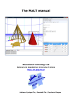
DECKBUILD’s process extraction window is shown below ( Figure 2-1:).
Figure 2-1: Process Extraction
SILVACO International
2-1
PC Interactive Tools User’s Manual
Users may use this window to look at:
•
Material thickness measures the thickness of the nth occurrence of any material or all materials
in the structure.
•
Junction depth measures the depth of any junction occurrence in the nth occurrence of any
material.
•
Surface concentration measures the surface concentration of any dopant, or net dopant, in the
nth occurrence of any material.
•
QUICKMOS 1D Vt calculates the one-dimensional threshold voltage of a MOS cross section using
the built-in QUICKMOS 1D device simulator. The gate voltage range defaults between 0 to 5 Volts
but can be specified as required, the substrate can also be fixed at any bias. Qss and device
temperature values may also be specified.
•
QUICKMOS CV curve creates a CV curve of a MOS cross section using QUICKMOS. Shows
capacitance as a function of either gate voltage or substrate voltage, with the other terminal held
at any fixed bias. Qss and device temperature values may also be specified.
•
QUICKBIP 1D solver measures any of 22 BJT Gummel-Poon parameters, plus any forward or
reverse IV curve. See the QUICKBIP subsection for more information and examples.
•
Junction capacitance versus bias calculates the junction capacitance of a specified p-n junction
within any region as a function of applied bias to that region. Qss and device temperature values
may also be specified.
•
Junction breakdown curve calculates the electron or hole ionization integral of any region as a
function of applied bias to that region. This calculation uses the Selberherr impact ionization
model (refer to “Impact” command section and “Impact Ionization” physics section within the
ATLAS manual). The Selberherr model default values may be modified if required plus, Qss and
device temperature values may be specified.
•
SIMS profile calculates the concentration profile of a dopant in a material layer.
•
SRP profile calculates the SRP (Spreading Resistance Profile) in a silicon layer.
•
Sheet resistance and sheet conductance calculates the sheet resistance or conductance of any
p-n region in any layer in an arbitrary structure. The bias of any region in any layer, the Qss of any
material interface and the device temperature may be specified. A flag for carrier freezeout
calculations may also be set (refer to “Incomplete Ionization Of Impurities” physics section within
the ATLAS manual).
•
Sheet resistance and sheet conductance versus bias calculates the sheet resistance or
conductance of one or more regions as a function of applied bias to any region. Qss and device
temperature values may also be specified.
•
Electrical concentration profiles. Measures electrical distributions versus depth. The bias of
any region in any layer and the Qss of any material interface may also be specified. The device
temperature may also be set to the required value. The following distributions are calculated:
— electrons
— holes
— electron quasi-fermi level
— hole quasi-fermi level
— intrinsic concentration
— potential
— electron mobility
— hole mobility
— electric field
— conductivity
2-2
SILVACO International
Extract Routines
•
1D maximum/minimum concentration measures the peak or minimum concentration of any
dopant or net dopant, for a specified 1D cutline, in the nth occurrence of any material or all
materials, and also within any junction-defined.
•
2D maximum/minimum concentration measures the peak or minimum concentration of any
dopant or net dopant, for the whole 2D structure or within a specified area, in any material or all
materials, and also within any junction-defined. The actual xy coordinates of the maximum or
minimum concentration may also be retrieved.
•
2D material region boundary returns the maximum or minimum boundary of the selected
material region for either X or Y axis. Hence the outer boundaries of any material region can be
extracted.
•
2D concentration area integrates specified concentration of any dopant or net dopant for whole
2d structure or within a specified location.
•
2D maximum concentration file (CCD) creates a Data Format file with the XY coordinates
and the actual values of the maximum concentrations stepping across the structure. This file may
be loaded into TONYPLOT when in -ccd mode to show a line of maximum concentration across a
device.
•
ED tree creates one branch of a Smile plot or ED tree from multiple Defocus distance against
Critical Dimension (CD) plots created for a sweep of Dose values by OPTOLITH. These plots are
all written in a single Data format file.
•
Elapsed time extracts time stamps from a specified start time at any point in a simulation, the
start time may be reset as required.
Note: This extraction is not CPU time.
The built-in 1D Poisson device simulator is used to calculate sheet resistance and conductance and the
electrical concentration profiles.
With the exception of 2D extractions, all the process extraction routines are available from both 1D
and 2D process simulators. In the case of the 2D simulators, a cross section x or y value or region name
(used in conjunction with MASKVIEWS) determines the 1D section to use.
Note: An error will be returned for attempted extractions on 3D structure files.
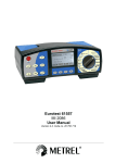
Entering a Process Extraction Statement
To place an extract statement in your process deck, activate the Extract... menu item on the
Commands menu. The Extraction popup appears. The popup for ATHENA is shown in Figure 2-2:
SILVACO International
2-3
PC Interactive Tools User’s Manual
Figure 2-2: The ATHENA Extraction Popup
Choose the extract routine you want by activating a choice on the Extract setting. The popup changes
size and display different items depending on which routine you choose. Then, enter or choose the
desired information for each item on the popup. An extract name is always be required. Optionally
enter the minimum or maximum desired cutoff values by checking Min value or Max value and
entering a value. By default, all extract results are written to a file named results.final, but using
the Results datafile field allows you to specify the results file for each individual extract statement.
Material and impurity names are selected using a Chooser (Figure 2-3:). If the required option is not
present in the default setting, select the User filter to search for other materials/impurities. The Hide
Worksheet Result setting specifies that this extract should not be displayed in the VWF INTERACTIVE
TOOLS worksheet. This prevents extracts used for calculation purposes only from cluttering the
worksheet results.
Finally, place the text caret at the desired point in the deck and click on the WRITE button. The
extract syntax is written to the deck.
Extracting a Curve
Some of the process extraction statements create a two-dimensional curve as a result, rather than a
single value. For instance, extract constructs a data set of concentration versus depth for the SIMS,
SRP, and electrical quantities distributions. The resulting 2-D curve can be used for measurement and
testing, and also as a target on the OPTIMIZER worksheet so that you can optimize against 2-D curves.
EXTRACT provides several additional options to 2-D curve support: axis layout, axis attributes, optional
computation of area under the curve, and optional outfile. These options are the same no matter what
type of curve (for instance, QUICKMOS CV and SIMS profile) the user is extracting.
The ATHENA Extract popup showing the SIMS Profile is shown in Figure 2-4: .
2-4
SILVACO International
Extract Routines
Figure 2-3: Material Chooser Popup
Figure 2-4: ATHENA Extract Popup with SIMS Profile
The following options are available:
X vs Y axis determines the x and y axes of the resulting profile curve. The default (which should
always be used unless the user plans to customize the resulting extract expression) is that the x axis is
depth into the material, and the y axis is the concentration.
Curve X axis bounds specifies whether to create the curve for the whole X axis or for only a required
section. If selected, X axis value fields become active, enter values in the same units as the resulting
curve. This is useful for extracting local maxima and minima.
X axis attributes and Y axis attributes allows the user to modify the data values on each axis
independently. To compute net concentration versus depth, the user might select abs on the y axis
(concentration), and select nothing on the x axis (depth). abs is always evaluated before taking the log
or square root of the data.
SILVACO International
2-5
PC Interactive Tools User’s Manual
Curve X axis bounds specifies whether to create the curve for the whole X axis or for only a required
section. If selected, X axis value fields become active, enter values in the same units as the resulting
curve. This is useful for extracting local maxima and minima.
Store X/Y datafile stores an output file in TONYPLOT data format if set to Yes. The user can plot the
data file in TONYPLOT using the -da option, and can also read the data file directly into the OPTIMIZER
worksheet as a target if desired.
Compute curve area is checked to compute the area under the curve. When checked, it causes
several other items to become active:
Area X axis bounds tells EXTRACT whether to integrate the area under the curve along its entire
length, or just for a bounded portion of the X axis. If Bounded is selected, then X axis start and X axis
stop become active. Enter start and stop values in the same units as the resulting curve.
To construct the 2-D curve, set each item on the popup in turn, then click on WRITE.
Depth is always computed as distance from the top of the selected material layer and occurrence.
Depth starts from 0 and increases through the material.
2-6
SILVACO International
Extract Routines
Customized Extract Statements
In addition to the simple curve primitives shown on the popup, the user can edit the input deck
directly to make customized curves. Examples include extracting maxima and minima on the curve,
combining axes via a function definition, looking at slopes of tangent lines, intercepts of sloped lines,
etc. The EXTRACT syntax is described below, followed by examples of process extraction, see the
examples listed under device extraction for more information.
Extract Syntax
General Syntax
extract init infile=<QSTRING>
extract <VALUE_TYPE>|<CURVE_TYPE> [name=<QSTRING>][outfile=<QSTRING>]
[datafile=<QSTRING>][hide][min.val=<EXPR>][max.val=<EXPR>]
extract start <TEST_SETUP 1>
[extract cont <TEST_SETUP N>]
extract done <VALUE_MUTLI_LINE>|<CURVE_MUTLI_LINE>[name=<QSTRING>]
[outfile=<QSTRING>][datafile=<QSTRING>][hide]
[min.val=<EXPR>][max.val=<EXPR>]
Description
<VALUE_TYPE> = <VALUE_SINGLE_LINE> | <VALUE_MULTI_LINE>
<VALUE_SINGLE_LINE> =
thickness
[<MATERIAL>][mat.occno=<EXPR>]
[y.val=<EXPR>|x.val=<EXPR>|region=<QSTRING>]
xj
[<MATERIAL>][mat.occno=<EXPR>][junc.occno=<EXPR>]
[y.val=<EXPR>|x.val=<EXPR>|region=<QSTRING>]
surf.conc
[<IMPURITY>][<MATERIAL>][mat.occno=<EXPR>]
[y.val=<EXPR>|x.val=<EXPR>|region=<QSTRING>]
1dvt
[ntype|ptype][bias=<EXPR>][bias.step=<EXPR>]
[bias.stop=<EXPR>][vb=<EXPR>]
[y.val=<EXPR>|x.val=<EXPR>|region=<QSTRING>]
[qss=<EXPR][workfunc=<EXPR>][soi][temp.val=<EXPR>]
max.conc |
[<IMPURITY>][<MATERIAL>][mat.occno=<EXPR>]
min.conc
[region.occno=<EXPR>]
[y.val=<EXPR>|x.val=<EXPR>|region=<QSTRING>]
2d.max.conc |
[<IMPURITY>][<MATERIAL>][mat.occno=<EXPR>]
2d.min.conc
[x.max=<EXPR> x.min=<EXPR> y.max=<EXPR> y.min=<EXPR> |
y.max=<EXPR> y.min=<EXPR> region=<QSTRING][interpolate]
x.pos |
y.pos
2d.conc.file
[<IMPURITY>][<MATERIAL>]
[x.max=<EXPR> x.min=<EXPR> y.max=<EXPR> y.min=<EXPR>]
max.bound |
x.val=<EXPR>|y.val=<EXPR>
min.bound(1D)
[<MATERIAL>][mat.occno=<EXPR>]
max.bound |
x.pos|y.pos x.val=<EXPR> y.val=<EXPR> [<MATERIAL>]
min.bound (2D)
2d.area
[<IMPURITY>][x.step=<EXPR>]
[x.max=<EXPR> x.min=<EXPR> y.max=<EXPR> y.min=<EXPR> |
y.max=<EXPR> y.min=<EXPR> region=<QSTRING]
SILVACO International
2-7
PC Interactive Tools User’s Manual
clock.time
[start.time=<EXPR>]
<VALUE_MULTI_LINE> =
sheet.res |
[material="silicon"|"polysilicon"][region.occno=<EXPR>]
p.sheet.res |
[mat.occno=<EXPR>][y.val=<EXPR>|x.val=<EXPR>|
region=<QSTRING>]
n.sheet.res |
[workfunc=<EXPR>][soi][semi.poly][incomplete]
[temp.val=<EXPR>]
conduct |
p.conduct |
n.conduct
<TEST_SETUP> =
CURVE_TYPE =
CURVE_DEF =
[<MATERIAL>][mat.occno=<EXPR>][region.occno=<EXPR>]
[bias=<EXPR>][y.val=<EXPR>|x.val=<EXPR>|region=<QSTRING>]
OR
[interface.occno=<EXPR>] [qss=<EXPR]
(<X_AXIS> , <Y_AXIS> [, x.min=<EXPR> x.max=<EXPR>])
where x.min and x.max define X limits of curve.
<X_AXIS> | <Y_AXIS> =
<AXIS>
<AXIS> + <EXPR>|<AXIS>
<AXIS> - <EXPR>|<AXIS>
<AXIS> / <EXPR>|<AXIS>
<AXIS> * <EXPR>|<AXIS>
<AXIS> ^ <EXPR>|<AXIS>
abs(<AXIS>) takes abs of all points along axis
log(<AXIS>) takes log of all points along axis
log10(<AXIS>) takes log10 of all points along axis
sqrt(<AXIS>) takes square root of all points along axis
atan(<AXIS>) takes arc tan of all points along axis
dydx(<AXIS>) calculates derivative of all points along axis
-<AXIS> inverts all points along axis
min(CURVE_DEF) returns min y val for curve
max(CURVE_DEF) returns max y val for curve
ave(CURVE_DEF) returns average value for curve.
slope|xintercept|yintercept(maxslope|minslope(CURVE_DEF)) Determines the
x or y intercept or returns the slope of the line.
area from (CURVE_DEF) [where x.min=<EXPR> and x.max=<EXPR>] Determines
area under specified curved between x-limits corresponding to values of min
and max expressions.
x.val from (CURVE_DEF) where y.val=<EXPR> [and val.occno=<EXPR>]
y.val from (CURVE_DEF) where x.val=<EXPR> [and val.occno=<EXPR>] Determines
the X[Y] coordinate on the curve where the corresponding Y[X] value is
equal to the constant expression for the occurence specified. Linear
interpolation is used between points on the curve.
grad from (CURVE_DEF) where x.val=<EXPR>|y.val=<EXPR> Determines the
gradient at the first X[Y] coordinate on the curve where the corresponding
Y[X] value is equal to the consent expression. Linear interpolation is used
between points on the curve.
<CURVE_DEF> = <CURVE_SINGLE_LINE> | <CURVE_MULTI_LINE>
2-8
SILVACO International
Extract Routines
<CURVE_SINGLE_LINE> =
curve(bias, 1dcapacitance [vg=<EXPR>][vb=<EXPR>][bias.ramp=<EXPR>]
[bias.step=<EXPR>][bias.stop=<EXPR>][temp.val=<EXPR>][soi]
[qss=<EXPR>] [workfunc=<EXPR>]
[y.val=<EXPR>|x.val=<EXPR>|region=<QSTRING>])
curve(depth, <IMPURITY>[<MATERIAL>]
[mat.occno=<EXPR>] [y.val=<EXPR>|x.val=<EXPR>|region=<QSTRING>])
curve(depth, srp [material="silicon"|"polysilicon"][mat.occno=<EXPR>]
[y.val=<EXPR>|x.val=<EXPR>|region=<QSTRING>])
curve(<VAR_AXIS> , <VAR_AXIS>)
deriv(<VAR_AXIS> , <VAR_AXIS> , <DERIVATIVE n>)
edcurve(<DEFOCUS_AXIS>, <CRITICAL_DIMENSION_AXIS>, <DOSE_AXIS>, dev=<EXPR>,
datum=<EXPR> x.step=<EXPR>)
<CURVE_MULTI_LINE> =
curve(bias, 1djunc.cap [<MATERIAL>][mat.occno=<EXPR>]
[region.occno=<EXPR>][junc.occno=<EXPR>][temp.val=<EXPR>]
[soi][qss=<EXPR>] [workfunc=<EXPR>]
[y.val=<EXPR>|x.val=<EXPR>|region=<QSTRING>])
<TEST_SETUP> = [<MATERIAL>][mat.occno=<EXPR>][region.occno=<EXPR>]
[bias=<EXPR>] [bias.step=<EXPR>][bias.stop=<EXPR>]
[y.val=<EXPR>|x.val=<EXPR>|region=<QSTRING>]
curve(bias, p.ion|n.ion [<MATERIAL>][mat.occno=<EXPR>]
[region.occno=<EXPR>][junc.occno=<EXPR>][temp.val=<EXPR>]
[soi][qss=<EXPR>] [workfunc=<EXPR>]
[y.val=<EXPR>|x.val=<EXPR>|region=<QSTRING>])
<TEST_SETUP> = [<MATERIAL>][mat.occno=<EXPR>][region.occno=<EXPR>]
[bias=<EXPR>] [bias.step=<EXPR>][bias.stop=<EXPR>]
[y.val=<EXPR>|x.val=<EXPR>|region=<QSTRING>]
curve(bias, 1dsheet.res|1dp.sheet.res|1dn.sheet.res|
1dconduct|1dp.conduct|1dn.conduct
[material="silicon"|"polysilicon"][region.occno=<EXPR>]
[mat.occno=<EXPR>][y.val=<EXPR>|x.val=<EXPR>|region=<QSTRING>]
[workfunc=<EXPR>][soi][semi.poly][incomplete][temp.val=<EXPR>]
<TEST_SETUP> =[<MATERIAL>][mat.occno=<EXPR>][region.occno=<EXPR>]
[bias=<EXPR>] [bias.step=<EXPR>][bias.stop=<EXPR>]
[y.val=<EXPR>|x.val=<EXPR>|region=<QSTRING>]
OR
[interface.occno=<EXPR>] [qss=<EXPR]
curve(bias, n.conc|p.conc|n.qfl|p.qfl|intrinsic|potential|n.mobility|
p.mobility|efield|econductivity
[material="silicon"|"polysilicon"][region.occno=<EXPR>]
[mat.occno=<EXPR>][y.val=<EXPR>|x.val=<EXPR>|region=<QSTRING>]
[workfunc=<EXPR>][soi][semi.poly][temp.val=<EXPR>]
<TEST_SETUP> =[<MATERIAL>][mat.occno=<EXPR>][region.occno=<EXPR>]
[bias=<EXPR>] [bias.step=<EXPR>][bias.stop=<EXPR>]
[y.val=<EXPR>|x.val=<EXPR>|region=<QSTRING>]
SILVACO International
2-9
PC Interactive Tools User’s Manual
OR
[interface.occno=<EXPR>] [qss=<EXPR]
<VAR_AXIS> =
v."<electrode>" - voltage at electrode
i."<electrode>" - current at electrode
c."<electrode1>""<electrode2>" - capacitance between electrode1 and
electrode2
g.”<electrode1>” “<electrode2>” - conductance between electrode1 and
electrode2
vint.“<electrode>” - internal voltage at electrode
time - transient time
temperature, temp - device temperature
frequency, freq - frequency
beam.“<beam no>” - light intensity for specified beam number
s.imaginary.“<Mode>” - imaginary value for specified “S” code
s.real.“<Mode>” - real value for specified “S” code
h.imaginary.“<Mode>” - imaginary value for specified “H” code
h.real.“<Mode>” - real value for specified “H” code
ie."<electrode>" - electron current
q."<electrode>" - charge
id."<electrode>" - displacement current
ireal."<electrode>" - real current
iimag."<electrode>" - imaginary current
ifn."<electrode>" - fowler nordhiem current
ihe."<electrode>" - hot electron current
ihh."<electrode>" - hot hole electron current
wfd."<electrode>" - workfunction difference
rl."<electrode>" - lumped resistance
cl."<electrode>" - lumped capacitance
ll."<electrode>" - lumped inductance
vcct.node."<circuit node>" - circuit bias
icct.node."<circuit node>" - circuit current
rhoe."<layer>" - Electron sheet resistance for layer
rhoh."<layer>" - Hole sheet resistance for layer
rho."<layer>" -Total sheet resistance for layer
vlayer."<layer>" - Bias on layer
sm."<mode>" - Photon density mode
pm."<mode>" - Laser power per mirror mode
gm."<mode>" - Gain mode
vcct.real."<circuit node>" - Real circuit bias
vcct.imag."<circuit node>" - Imaginary circuit bias
icct.real."<circuit node>" - Real circuit current
icct.imag."<circuit node>" - Imaginary circuit current
abcd.real."<mode>" - ABCD real parameter
abcd.imag."<mode>" - ABCD imaginary parameter
y.real."<mode>" - Y real parameter
y.imag."<mode>" - Y imaginary parameter
z.real."<mode>" - Z real parameter
z.imag."<mode>" - Z imaginary parameter
probe."<probe name>" - Atlas probe values
elect.“<parameter>” - Value for specified electrical parameter
“<parameter>”=
time - Light frequency
freq - frequency
2-10
SILVACO International
Extract Routines
temp - temperature
current gain - unilateral power
gain frequency - max transducer
power gain - luminescent power
luminescent wavelength - optical source frequency
available photo current - source photo current,
optical wavelength - position xhole mobility
Time step magnitude -Time step number
Total integration time - Cutoff frequency
Distance along line - Norm Intensity
Integrated e- Conc - Integrated h+ Conc
Channel Sheet Conductance - Photon Energy
Photon Density - Gain
Spontaneous emission rate - electron mobility
hole current - generation rate
lattice temp - electric field
recombination rate - displacement current
electron conc - hole conc
rlectron temp - hole temp
relative permitivity - potential
da.value"<CURVE_NUMBER>""<DA_FILE_AXIS>"
da.value"<DA_FILE_AXIS>"
Note: <CURVE_NUMBER> is to specify which curve when multiple curves are present in a DA format file.
<IMPURITY>
boron
antimony
arsenic
phosphorus
net
OR
impurity = <QSTRING> (eg. impurity="electron conc")
Note: See Deckbuild ATHENA Extract popup Impurity Chooser for list of impurity strings
<MATERIAL> =
gas
silicon
oxide
polysilicon
aluminum
nitride
oxynitride
gaas
gold
silver
alsi
photoresist
tungsten
titanium
platinum
tisix
SILVACO International
2-11
PC Interactive Tools User’s Manual
wsix
ptsix
OR
material = <QSTRING> (eg. material ="algaas")
Note: See Deckbuild ATHENA Extract popup Material Chooser for list of material strings
<QSTRING> = quoted string (eg. "Silicon")
<LINE> = returned value from maxslope or minslope.
<EXPR> =
number - real or integer value)
$variable | $"variable" - deckbuild set variable
expr + expr
expr - expr
expr / expr
expr * expr
min (<AXIS>) - returns min value of var over its range
max (<AXIS>) - returns max value of var over its range
ave (<AXIS>) - returns ave value of var over its range
slope (<LINE>) - returns a where y = ax + b
yintercept (<LINE>) - returns b where y = ax + b
xintercept (<LINE>) - returns -b/a where y = ax + b
register = expr - sets register value
register - returns value of set register
(expr)
-expr
DEFAULTS
For optional extract arguments which are specified, the following default values apply:
material = "silicon"
impurity = "net doping"
x.val|y.val|region - x.val = 5% of device size from left hand side.
*.occno = 1
datafile="results.final"
1dvt type = ntype
2d.area x.step = 10% of device size
temp.val = 300
bias=0
1dvt - bias.stop = 5, bias.step = 0.25, vb=0
1dcapacitance - bias.stop = 5, bias.step = 0.25, vb=0, vg=0, bias.ramp=vg
soi = FALSE
semi.poly = FALSE
incomplete = FALSE
Examples of Process Extraction
Note: Extract commands maybe entered on multiple lines using a backslash character for continuation, but the syntax shown
below should be entered on a single line although shown on two or more lines.
2-12
SILVACO International
Extract Routines
The following examples assume to be extracting values from the current simulation running under
DECKBUILD, but saved standard structure files may be used directly with extract using the syntax
below:
extract init infile="filename“
Material Thickness
Extract the thickness of the top (first) occurrence of Silicon Oxide for a 1D cutline taken where Y=0.1
(Assume 2D structure), a warning is then displayed if results cross boundaries set by max.v and min.v.
extract name="tox" thickness material="SiO~2" mat.occno=1 y.val=0.1
min.v=100 max.v=500
(oxide can be substituted for the material="SiO~2")
Junction Depth
Extract the junction depth of the first junction occurrence in the top (first) occurrence of silicon for a
1D cutline taken where X=0.1.
extract name="j1 depth" xj material="Silicon" mat.occno=1 x.val=0.1
junc.occno=1
Surface Concentration
Extract the surface concentration net doping for the top (first) occurrence of silicon for a 1D cutline
taken for an X value corresponding to the gate contact/region for loaded MASKVIEWS cutline data.
extract name="surface conc" surf.conc impurity="Net Doping"
material="Silicon" mat.occno=1 region="gate"
QUICKMOS 1D Vt
Extract the 1D threshold voltage of a p-type MOS cross section at x=0.1 using the built-in QUICKMOS
1D device simulator. This example uses a default gate bias setting of 0-5V for a 0.25V step with the
substrate at 0V and a default device temperature of 300 Kelvin. Values of QSS and gate workfunction
have also be specified.
extract name="1D Vt" 1dvt ptype qss=1e10 workfunc=5.09 x.val=0.1
This 1D Vt extraction will calculate the 1D threshold voltage of an n-type MOS cross section at X=0.1
where a gate voltage range (0.5-20V) has been specified while the substrate (Vb) is set at 0.2V. The
device temperature has been set to 350 Kelvin.
extract name="1D Vt 0-20v" 1dvt ntype bias=0.5 bias.step=0.25 bias.stop=20.0
vb=0.2 temp.val=350.0 x.val=0.1
SILVACO International
2-13
PC Interactive Tools User’s Manual
Sheet Resistance and Sheet Conductance
Note: For sheet conductance extraction substitute “sheet.res” with “conduct” (i.e, conduct, p.conduct, n.conduct)
Extract the total sheet resistance of the first p-n region in the top (first) occurrence of polysilicon for a
cutline at X=0.1. Polysilicon is treated as a metal by default but is flagged here as a semiconductor
(semi.poly). The default device temperature of 300 Kelvin and no layer biases will be used and the
incomplete ionization flag is also set for carrier freezeout calculations (refer to “Incomplete Ionization
Of Impurities” physics section within the ATLAS manual).
extract name="Total SR" sheet.res material="Polysilicon" mat.occno=1
x.val=0.1 region.occno=1 semi.poly incomplete
Extract the n-type sheet resistance of the second p-n region in the top (first) occurrence of silicon for a
cutline at X=0.1 where the second region is held at 4.0V and the device temperature is set to 325
Kelvin. These commands use the start/cont/done syntax to create a multi-line statement as
described in the Extract features section.
extract start material="Silicon" mat.occno=1 region.occno=2 bias=4.0
x.val=0.1 extract done name="N-type SR" n.sheet.res material="Silicon"
mat.occno=1 temp.val=325 x.val=0.1 region.occno=2
The following multi-line statement extracts the p-type sheet resistance of the first p-n region in the top
(first) occurrence of silicon for a cutline at x=0.1 where the first region is held at 5.0V, the second
region is held at 1.0V and the first interface Qss value equal to 1e10.
extract start material="Silicon" mat.occno=1 region.occno=1 bias=5.0
x.val=0.1
extract cont material="Silicon" mat.occno=1 region.occno=2 bias=1.0
x.val=0.1
extract cont interface.occno=1 qss=1.0e10
extract done name="P-type SR" p.sheet.res material="Silicon" mat.occno=1
x.val=0.1 region.occno=1
Note: This is an example of the multi-line “start/continue/done” type of statement used to specify layer biases and Qss values.
It is recommended that the user always let the Extract popup write this particular syntax. The Qss value also specifies the
material interface occurrence involved, counting from the top down. There can be any number of additional “continue” lines to
specify the biases on other layers and the Qss values of other interfaces; the last line, “done”, does the actual extraction.
1D Max/Min Concentration
Extract the peak concentration of net doping within the first p-n region of the top (first) layer of silicon
for a 1D cutline at x=0.1.
extract name="Max 1d Net conc" max.conc impurity="Net Doping"
material="Silicon" mat.occno=1 x.val=0.1 region.occno=1
Extract the peak concentration of phosphorus within any p-n regions (default) for all materials using a
1D cutline at x=0.1.
extract name="Max 1d phos conc" max.conc impurity="Phosphorus"
material="All" x.val=0.1
Extract the minimum concentration of boron within any p-n regions of the top (first) layer of silicon for
a 1D cutline at x=0.1.
2-14
SILVACO International
Extract Routines
extract name="Min 1d bor conc" min.conc impurity="Boron" material="Silicon"
mat.occno=1 x.val=0.1
2D Max/Min Concentration
Extract the peak concentration of net doping for the entire 2D structure.
extract name="Max 2D net conc" 2d.max.conc impurity="Net Doping"
material="All"
Extract the peak concentration of boron within the silicon material in the 2D “box” limits defined.
extract name="Max 2D bor conc" 2d.max.conc impurity="Boron"
material="Silicon" y.min=0.1 y.max=0.9 x.min=0.2 x.max=0.6
In addition to this statement the interpolate flag may be added. When present, this flag causes the
extraction to perform interpolation at the edges of the specified bounding box for min/max
concentration and position.
Extract the minimum concentration of phosphorus for all materials within the 2D “box” limits. These
limits are defined by user defined y coordinates and x values corresponding to loaded MASKVIEWS
cutline information for the specified electrode or region.
extract name="Min 2D phos conc" 2d.min.conc impurity="Phosphorus"
material="All" region="gate" y.min=0.1 y.max=0.9
The following multi-line extract command measures the minimum concentration of antimony for the
entire 2D structure and return the x-y coordinates of the extracted concentration.
extract name="Min 2D ant conc" 2d.min.conc impurity="Antimony"
material="All"
extract name="Min 2D ant conc X position" x.pos
extract name="Min 2D ant conc Y position" y.pos
Note: The x-y position syntax must directly follow the 2D concentration extraction (same as start/continue/done syntax), it is
advisable to use the Extract popup to create these statements.
2D Concentration File
The output file contains data of the format x y c where c is the value of concentration at the
coordinates xy. The following example extracts the boron concentration in Silicon for the whole
structure.
extract 2d.conc.file material="silicon" impurity="boron" outfile="conc.dat"
1D Material Region Boundary
Extracting the maximum Y boundary (upper side) location of the first occurrence of silicon material for
a 1d cutline taken at X=2.
extract name="max_y" max.bound material="silicon" x.val=2 mat.occno=1
Extracting the minimum X boundary (left side) location of the second occurrence of polysilicon
material for a 1d cutline at Y=3.
extract name="min_x" min.bound material="polysilicon" y.val=3 mat.occno=2
2D Material Region Boundary
Extracting the minimum X boundary (left side) location of the photoresist material region at XY
coordinates (7.6, -1.2).
SILVACO International
2-15
PC Interactive Tools User’s Manual
extract name="minx" min.bound x.pos material="photoresist" x.val=7.6 y.val=1.2
Extracting the maximum Y boundary (upper side) location of the photoresist material region at XY
coordinates (5.2, 0).
extract name="maxy" max.bound y.pos material="photoresist" x.val=5.2 y.val=0
2D Material Region Boundary
Extracting the minimum X boundary (left side) location of the photoresist material region at XY
coordinates (7.6, -1.2).
extract name="minx" min.bound x.pos material="photoresist"
x.val=7.6 y.val=-1.2
Extracting the maximum Y boundary (upper side) location of the photoresist material region at XY
coordinates (5.2, 0)
extract name="maxy" max.bound y.pos material="photoresist"x.val=5.2 y.val=0
2D Concentration Area
Integrates the Boron concentration within the specified “box” limits, using a cutline step of 0.05
microns.
extract name="limit_area" 2d.area impurity="Boron" x.step=0.05 x.min=0.01
y.min=0.23 x.max=0.6 y.max=0.45
In addition to this statement, the interpolate flag may be added. When present, this flag causes the
extraction to perform interpolation at the edges of the specified bounding box for min/max
concentration and position.
Integrates the Phosphorus concentration for the whole 2D structure using a cutline step of 0.03
microns.
extract name="device_area" 2d.area impurity="Phosphorus" x.step=0.03
Note: The x.step refers to the number of 1d cutlines used to obtain the 2d area. For a device with an X axis of 7 microns an
x.step of 1 would result in 8 cutlines being used at 1 micron intervals.
2D Maximum Concentration File
Creates a Data format file plotting the position of the maximum potential, in silicon material only, for
the whole 2D structure. A maximum potential Y position is found for every X step of 0.1 microns.
These Data format files may be loaded into TONYPLOT (-ccd) to represent a line of maximum
concentration across a device.
extract name="Total_max_pot" max.conc.file impurity="potential" x.step=0.1
material="silicon" outfile="totalconc.dat"
Creates a Data format file plotting the position of the maximum potential, in any material, for the
specified “box” limits. A maximum potential Y position is found for every X step of 0.2 microns.
extract name="limit_max_pot" max.conc.file impurity="potential"
x.step=0.2 outfile="limitconc.dat" x.min=0 x.max=7 y.min=0 y.max=0.09
Note: The x.step does not refer to cutlines but to the number of X coordinates used. A value of 1 representing stepping 1
micron in X for every max Y value calculated.
2-16
SILVACO International
Extract Routines
QUICKMOS CV Curve
Extract a MOS CV curve, ramping the gate from 0 to 5 volts, with 0 volts on the backside and the
device temperature set at 325 Kelvin (default 300 K). This example creates a curve that is stored in file
cv.dat, and can be shown using TONYPLOT. (To bring up TONYPLOT on this file, an easy way is to
highlight the file name and then click on DECKBUILD’s Tools button. TONYPLOT starts and is loaded with
the file automatically).
extract name="CV curve" curve(bias,1dcapacitance vg=0.0 vb=0.0 bias.ramp=vg
bias.step=0.25 bias.stop=5.0 x.val=0.1 temp.val=325) outfile="cv.dat"
To get the maximum capacitance for the same curve, insert the keyword max (by editing the syntax
created by the popup). Notice that in this example, a single value is being extracted from a curve, not
the curve itself. However, the user still store the curve used during the calculation into an output file
— this is always the case.
extract name="CV curve Max cap" max(curve(bias,1dcapacitance vg=0.0 vb=0.0
bias.ramp=vg bias.step=0.25 bias.stop=5.0 x.val=0.1 temp.val=325))
outfile="cv.dat"
To find what the capacitance was at voltage 4.3 volts, use the following syntax:
extract name="MOS capacitance at Vg=4.3" y.val from curve(bias,1dcapacitance
vg=0.0 vb=0.0 bias.ramp=vg bias.step=0.25 bias.stop=5.0 x.val=0.1
temp.val=325) where x.val = 4.3
The general form of this syntax is
extract y.val from curve(xaxis, yaxis) where x.val=number_on_xaxis
and:
extract x.val from curve(xaxis, yaxis) where y.val=number_on_yaxis
where xaxis and yaxis will determine the actual curve. The syntax for this example was created by
using the popup to write the syntax for the CV curve, and then adding the y.val... where x.val syntax in
the input deck.
For more examples on how to manipulate curves, see the examples in the Device Extraction section.
Junction Capacitance Curve
Extract a curve of junction capacitance against bias where the first region in the top (first) layer of
silicon is ramped from 0 to 5V. Capacitance of the first junction occurrence (upper) is measured and the
resultant curve is output to the file XjV.dat. Device temperature is default (300 Kelvin). If only one
junction exists for the selected region then a junction occurrence of one (upper) must be used.
extract start material="Silicon" mat.occno=1 bias=0.0 bias.step=0.25
bias.stop=5.0 x.val=0.1 region.occno=1
extract done name="Junc cap vs bias" curve(bias,1djunc.cap
material="Silicon" mat.occno=1 x.val=0.1 region.occno=1 junc.occno=1)
outfile="XjV.dat"
Extract the minimum junction capacitance on the created junction capacitance against bias curve. The
second region in the top (first) layer of silicon is ramped from 0 to 3V and the capacitance of the second
junction occurrence (lower) is measured. Device temperature is set for calculations to be 325 Kelvin.
The resultant curve is output to the file XjVmin.dat, while the extracted minimum value is logged to
the default results file (results.final).
extract start material="Silicon" mat.occno=1 bias=0.0 bias.step=0.25
bias.stop=3.0 x.val=0.1 region.occno=2
extract done name="Junc cap vs bias" min(curve(bias,1djunc.cap
material="Silicon" mat.occno=1 x.val=0.1 region.occno=2 junc.occno=2
SILVACO International
2-17
PC Interactive Tools User’s Manual
temp.val=325)) outfile="XjVmin.dat"
Note: The junction occurrence is only valid for the specified region, i.e., there is only a maximum of two possible junctions for
the specified region.
Junction Breakdown Curve
Extract a curve of electron ionization integral against bias where the first region in the top (first) layer
of silicon is ramped from 0 to 5V and device temperature is set to be 325 Kelvin. The resultant
breakdown curve is output to the file Nbreakdown.dat. (Refer to “Impact” command section and
“Impact Ionization” physics section within the ATLAS manual for the Selberherr model used in
calculation).
extract start material="Silicon" mat.occno=1 bias=0.0 bias.step=0.25
bias.stop=5.0 x.val=0.1 region.occno=1
extract done name="N Breakdown “curve(bias,n.ion material=”Silicon"
mat.occno=1 x.val=0.1 region.occno=1 temp.val=325)
outfile="Nbreakdown.dat"
The following extraction creates a curve of hole ionization integral against bias, and calculates the
breakdown voltage corresponding to the point where the hole ionization integral intercepts 1.0. The
second region in the top (first) layer of silicon is ramped from 0 to 20V and the device temperature is
set to the default of 300 Kelvin. The resultant breakdown curve is output to the file Pbreakdown.dat
and the breakdown voltage is appended to the default results file (results.final).
extract start material="Silicon" mat.occno=1 bias=0.0 bias.step=0.50
bias.stop=20.0 x.val=0.1 region.occno=2
extract done name="P intercept" x.val from curve(bias,p.ion
material="Silicon" mat.occno=1 x.val=0.1 region.occno=2) where y.val=1.0
outfile="Pbreakdown.dat"
Selberherr model parameters can be modified using the syntax shown below. More details are provided
in the Models and Algorithms section of Appendix A.
extract start material="Silicon" mat.occno=1 bias=0.2 bias.step=0.08
bias.stop=5.0 x.val=0.3 region.occ=2
extract done name="iiP" curve(bias, p.ion material="Silicon" mat.occno=1
x.val=0.3 region.occno=2 egran=4.0e5 betap=1.0 betan=1.0
an1=7.03e5 an2=7.03e5 bn1=1.231e6 bn2=1.231e6 ap1=6.71e5 ap2=1.582e6
bp1=1.693e6 bp2=1.693e6) outfile="extract.dat"
SIMS Curve
Extract the concentration profile of net doping in the top (first) layer of silicon. The output curve is
placed into the file SIMS.dat.
extract name="SIMS" curve(depth,impurity="Net Doping" material="Silicon"
mat.occno=1 x.val=0.1) outfile="SIMS.dat"
SRP Curve
Extract the SRP (Spreading Resistance Profile) in the top (first) silicon layer. The output curve is
placed into the file SRP.dat.
extract name="SRP" curve(depth, srp materials="Silicon" mat.occno=1
x.val=0.1)
2-18
SILVACO International
Extract Routines
outfile="SRP.dat"
The following command will calculate the SRP (Spreading Resistance Profile) in the top (first) silicon
layer using a specified 100 etch steps of uniform size. The output curve is placed into the file
SRP100.dat.
extract name="SRP100" curve(depth,srp material="Silicon"
mat.occno=1 n.step=100 x.val=0.5) outfile="srp100.dat"
Note: Where n.step not specified the default is 50 etch steps of variable size dependent on the gradient of net concentration.
If n.steps is set, uniform etch steps are used.
Sheet Resistance/Conductance Bias Curves
Extract the Total sheet conductance against bias curve of the first p-n region in the top (first)
occurrence of polysilicon. Polysilicon is treated as a metal by default but is flagged here as a
semiconductor (semi.poly). The device temperature is set to 325 Kelvin (default=300 Kelvin) and a bias
ramped from 0 to 5V on the same polysilicon region.
extract start material="Polysilicon" mat.occno=1 bias=0.0 bias.step=0.00
bias.stop=5.0 x.val=0.1 region.occno=1
extract done name="Total SC" curve(bias,1dconduct material="Polysilicon"
mat.occno=1 temp.val=325 x.val=0.1 region.occno=1 semi.poly)
outfile="totalSC.dat"
Extract the n-type sheet conductance against bias curve of the first p/n region in the top (first)
occurrence of silicon where a bias ramped from 0V to 5V on the same silicon region and a value of QSS
(4.0e10) is specified for the first interface occurrence.
extract start material="Silicon" mat.occno=1 region.occno=1 bias=0.0
bias.step=0.00 bias.stop=5.0 x.val=0.1
extract cont interface.occno=1 qss=4.0e10
extract done name="N-type SC" curve(bias,1dn.conduct material="Silicon"
mat.occno=1 x.val=0.1 region.occno=1) outfile="NtypeSC.dat"
Extract the p-type sheet conductance against bias curve of the first p-n region in the top (first)
occurrence of silicon where a bias ramped from 0 to 5V on the same silicon region and a bias of 2V is
held on the first region of the top occurrence of polysilicon. A value of QSS (5.0e10) is also specified for
the first interface occurrence.
extract start material="Silicon" mat.occno=1 region.occno=1 bias=0.0
bias.step=0.00 bias.stop=5.0 x.val=0.1
extract cont material="Polysilicon" mat.occno=1 bias=2.0 x.val=0.1
region.occno=1
extract cont interface.occno=1 qss=5.0e10
extract done name="P-type SC" curve(bias,1dp.conduct material="Silicon"
mat.occno=1 x.val=0.1 region.occno=1) outfile="PtypeSC.dat"
The command below extracts the p-type sheet conductance against bias curve of the first and second pn regions in the top (first) layer of silicon where a bias is ramped from 1V to -2V on the top (first)
polysilicon layer.
extract start material="Polysilicon" mat.occno=1 bias=1.0 bias.step=-0.05
bias.stop=-2.0 x.val=0.01
extract done name="region1+2" curve(bias,1dp.conduct material="Silicon"
mat.occno=1 x.val=0.01 region.occno=1 region.stop=2) outfile="region1+2.dat"
SILVACO International
2-19
PC Interactive Tools User’s Manual
Note: For sheet resistance extraction substitute “1dconduct” with “1dsheet.res” (i.e. 1dsheet.res, 1dnsheet.res, 1dpsheet.res)
Electrical Concentration Curve
Extract the electron distribution against depth for the top (first) layer of silicon where a bias is ramped
from 0 to 5V for the first region of the silicon and a QSS of 4.0e10 set for the first interface occurrence.
Device temperature is set at 325 Kelvin.
extract start material="Silicon" mat.occno=1 region.occno=1 bias=0.0
bias.step=0.00 bias.stop=5.0 x.val=0.1
extract cont interface.occno=1 qss=4.0e10
extract done name="Electrical conc" curve(depth,n.conc material="Silicon"
mat.occno=1 x.val=0.1 temp.val=325) outfile="extract.dat"
ED Tree (Optolith)
Creates a Data format file plotting a single branch of an ED tree for deviation of 10% from the datum,
the specified critical dimension (CD) value of 0.5. The x.step defines the defocus step to be used, 0.08
representing 8% of the total X axis range for each calculation. For each value of defocus at the specified
critical dimension deviation, the value of dose is interpolated. Hence, the resulting curve is dose
against defocus for a critical dimension of 0.5 plus 10%.
extract name="ed+10" edcurve(da.value."DEFOCUS", da.value."CDs",
da.value."DOSE",dev=10 datum=0.5 x.step=0.08) outf="ed10.dat"
Note: If no x.step is specified the actual curve defocus points are used.
Elapsed time
The timer is reset to 10 seconds, a timestamp extracted before and then after a simulation. The
elapsed time is then calculated by subtraction.
extract name ="reset_clock" clock.time start.time = 10
extract name ="t1" clock.time
<simulation>
extract name ="t2" clock.time
extract name="elapsed_time" $t2 - $t1
Note: This extraction does not measure CPU time
2-20
SILVACO International
Extract Routines
Device Extraction
Device extraction always deals with a “logfile” that contains I-V information produced by a device
simulator (such as ATLAS), and therefore deals almost exclusively in curves. The following section
show how to construct a curve or extract values on a curve for all possible devices. (For the special case
of MOS devices, both ATLAS and SMINIMOS4 have popups with a number of pre-defined MOS tests.
See MOS Device Tests.)
Device extraction also deals with structure files which contain information saved by a device simulator
(i.e., ATLAS). This information may be extracted by using the process extraction syntax style shown
below. The following extracts the total electric field for silicon in a 1-D cutline where x = 0.5 for the
loaded device structure file.
extract name="test" 2d.max.conc impurity="E Field" material="Silicon"
x.val=0.5
There are some differences between the syntax used by EXTRACT and the syntax used by the ATLAS
output command. These differences are documented in Appendix B of this manual.
Extract allows the user to construct a curve using separate X and Y axes. For each axis, the user can
choose the voltage or current on any electrode, the capacitance or conductance between any two
electrodes, or the transient time for AC simulations. The axes may be manipulated individually, such
as multiplication or division by a constant, or axes may be combined in algebraic functions.
Note: Note that the curve manipulation discussed is equally applicable to all curves, whether the curve came from process or
device simulation. The only type-specific syntax relates to the curve axes; i.e., gate voltage can’t be extracted from a process
simulator, etc. If this is attempted, a warning message is printed.
The Curve
The basic element is always the curve. Once the curve is constructed, it can be used as is, by saving it
to a file for use by TONYPLOT, or as an OPTIMIZER target, or it can be used as the basis for further
extraction. For details on the EXTRACT curve syntax, see the Extract Syntax Description section earlier
in this chapter.
To construct a curve representing voltage on electrode “emitter1” (on the X axis) versus current on
electrode “base2", write:
extract name="iv" curve(v."emitter1", i."base2")
The first variable specified inside the parentheses becomes the X axis of the curve; the second variable
becomes the Y axis. The v.“name” and i.“name” syntax is used for any electrode name — just insert the
proper name of the electrode. The electrode name must have been defined previously (such as in the
device deck, or previous to that in an ATHENA input deck using the “electrode” statement, or
interactively in DEVEDIT). Electrode names may contain spaces but must always be quoted.
Transient time is represented by keyword time:
extract name="It curve" curve(time, i."anode")
For Device temperature curves use:
extract name="VdT" curve(v."drain", temperature)
For extracting a frequency curve use:
extract name="Idf" curve(i."drain", frequency)
To extract a capacitance or conductance curve, use this syntax:
SILVACO International
2-21
PC Interactive Tools User’s Manual
extract name="cv" curve(c."electrode1""electrode2", v."electrode3")
and
extract name="gv" curve(g."electrode1""electrode2", v."electrode3")
For other electrical parameters (refer to Extract Syntax section for valid electrical parameters) use the
following syntax:
extract name="IdT" curve(elect."parameter“,v.”drain")
An extract name is given in each example. Although not strictly required, it is always a good idea to
name extract statements so they can be identified later. Names are always necessary for entering an
extract statement in DECKBUILD’s OPTIMIZER, and for recognition by the VWF.
It is also possible to shift or manipulate curve axes. Each axis is manipulated separately. The simplest
form of axis manipulation is algebra with a constant:
extract name="big iv" curve(v."gate"/50, 10*i."drain")
Any constant expression can be multiplied, divided, added, or subtracted to each axis.
Curve axis may also be combined algebraically, similar to TONYPLOT’s function capability:
extract name="combine" curve(i."collector", i."collector"/i."base")
All electrode values (current, voltage, capacitance, conductance) may be combined in any form this
way.
Another curve type is deriv() used to return the derivative (dydx). For example, statement below will
create the curve of dydx gate bias and drain current plotted against and X axis of gate bias.
extract name="dydx" deriv(v."gate", i."drain")
outfile="dydx.dat"
It is also possible to calculate dydx to the nth derivative as below:
extract name="dydx2" deriv(v."gate", i."drain", 2)
outfile="dydx2.dat"
To find local maxima and minima on a curve, the section of the curve X axis can be limited. The
following statement extracts the maximum drain current where gate bias is between the limits of 0.5
volts and 2.5 volts.
extract name="limit" max(curve(v."gate", i."drain",x.min=0.5
x.max=2.5)) outf="limit.dat"
In addition, there are several operators which apply to curve axes. They are:
abs(axis)
log(axis)
log10(axis)
sqrt(axis)
atan(axis)
-axis
For instance:
extract curve(abs(i."drain"), abs(v."gate"))
The operators may be combined, i.e., log10(abs(axis)). These operators work on curve axes from
process simulation as well.
2-22
SILVACO International
Extract Routines
Curve Manipulation
A number of curve manipulation primitives exist:
min(curve)
max(curve)
ave(curve)
minslope(curve)
maxslope(curve)
slope(line)
xintercept(line)
yintercept(line)
area from curve
area from curve where x.min=X1 and x.max=X2
x.val from curve where y.val=k
y.val from curve where x.val=k
x.val from curve where y.val=k and val.occno=n
y.val from curve where x.val=k and val.occno=n
grad from curve where y.val=k
grad from curve where x.val=k
For details of Extract curve manipulation syntax, see the Extract Syntax Description section earlier in
this chapter.
For instance, using the BJT curve example above, the user could find the maximum of Ic/Ib vs Ic, or
maximum beta, by writing:
extract name="max beta" max(curve(i."collector", i."collector"/i."base"))
max(), min(), and ave() all work on the Y axis of the curve.
The sloped lines and intercepts often work together. The primitives minslope() and maxslope() can be
thought of as returning a line. Extracting a line by itself has no meaning, so three other operators take
a line as input. The operators are slope(), which returns the slope of the line, and xintercept() and
yintercept(), which return the value where the line intercepts the corresponding axis.
For instance, a Vt test for MOS devices looks at a curve of Vg (x) versus Id (y), and finds the X
intercept of the maximum slope. Such a test would look like:
extract name="vt" xintercept(maxslope(curve(abs(v."gate", abs(i."drain"))))
Some Vt tests take off Vd/2 from the resulting value. You could write:
extract name="vt" xintercept(maxslope(curve(abs(v."gate",
abs(i."drain")))) - ave(v."drain")/2
Note that the last example uses:
ave(v."drain")/2
The min(), max(), and ave() operators can be used on both curves,
extract name="Iave" ave(curve(v."gate", i."drain"))
and also on individual curve axes,
extract name="Iave" ave(i."drain")
or even on axis functions:
extract name="Icb max" max(i."collector"/i."base")
SILVACO International
2-23
PC Interactive Tools User’s Manual
The user can also find the Y value on a curve for a given X value, and the other way round. For
example, to find the collector current (Y) for base voltage 2.3 (X), use:
extract name="Ic[Vb=2.3]" y.val from curve(abs(v."base"),
abs(i."collector")) where x.val = 2.3
EXTRACT uses linear interpolation if necessary. If more than one point on the curve matches the
condition, the first one is taken, unless the following syntax is used to specify the occurrence of the
condition. This example would find the second Y point on the curve matching an X value of 2.3:
extract name="Ic[Vb=2.3]" y.val from curve(abs(v."base",
abs(i."collector"))
where x.val = 2.3 and val.occno =2
The condition used for finding an intercept can be a value or an expression and therefore use the min(),
max(), and ave() operators. The following command creates a transient time against drain-gate
capacitance curve and calculate the intercepting time where the capacitance is at its minimum value:
extract name="t at Cdrain-gate[Min]" x.val from curve(time, c."drain""gate")
where y.val=min(c."drain""gate")
In addition to finding intercept points on curves, it is possible to calculate the gradient at the
intercept, specified by either a Y or X value, as shown below:
extract name="slope_at_x" grad from curve(v."gate", i."drain")
where x.val=1.5
extract name="slope_at_y" grad from curve(v."gate", i."drain")
where y.val=0.001
It is also possible to find the area under a specified curve for either the whole curve or as below,
between X limits:
extract name="iv area" area from curve(v."gate", c."drain""gate")
where x.min=2 and x.max=5
2-24
SILVACO International
Extract Routines
General Curve Examples
The following examples assume that they are extracting values from the currently loaded logfile
running under DECKBUILD, but saved “IV” log files maybe used directly with extract using the syntax
below:
extract init infile="filename“
Note: Extract commands maybe entered on multiple lines using a backslash character for continuation, but the syntax shown
below should be entered on a single line although shown on two or more lines.
Curve Creation
The following command extracts a curve of collector current against base voltage and places the output
in icvb.dat.
extract name="IcVb curve" curve(i."collector", v."base") outfile="icvb.dat"
Min Operator with Curves
The following command calculates the minimum value for a curve of drain current against internal
gate voltage.
extract name="Vgint[Min]" min(curve(i."drain", vint."gate"))
Max Operator with Curves
The following command calculates the maximum value for a curve of base voltage against basecollector capacitance.
extract name="Cbase-coll[Max]" max(curve(v."base", c."base""collector"))
Ave Operator with Curves
The following command calculates the average value for a curve of drain current against gate-drain
conductance.
extract name="Ggate-drain[Ave]" ave(curve(i."drain", g."gate""drain"))
X Value Intercept for Specified Y
The following command creates a frequency against drain current curve and calculate the intercepting
frequency for a drain current of 1.5-e6.
extract name="Freq at Id=1.5e-6" x.val from curve(frequency, i."drain") where
y.val=1.5e-6
Y Value Intercept for Specified X
The following command creates a drain voltage against device temperature curve and calculates the
intercepting temperature for a drain voltage of 5V.
extract name="T at Vd=5" y.val from curve(v."drain", temperature) where
x.val=5.0
SILVACO International
2-25
PC Interactive Tools User’s Manual
Abs Operator with Axis
The following command creates a curve of absolute gate voltage against absolute optical wavelength
(log, log10 and sqrt also available).
extract name="Vg-optW curve" curve(abs(v."gate"), abs(elect."optical
wavelength"))
Min Operator with Axis Intercept
The following command creates a transient time against gate-drain capacitance curve and calculate
the intercepting time where the capacitance is at its minimum value.
extract name="t at Cgate-drain[Min]" x.val from curve(time, c."gate""drain")
where y.val=min(c."gate""drain")
Max Operator with Axis Intercept
The following command creates a collector current against collector current divided by base current
curve and calculate the intercepting collector current where Ic/Ib is at a maximum value.
extract name="Ic at Ic/Ib[Max]" x.val from curve(i."collector",
i."collector"/i."base") where y.val=max(i."collector"/i."base")
Second Intercept Occurrence
The following command creates a gate voltage against source photo current curve and calculates the
second intercept of gate voltage for a source photo current of 2e-4.
extract name="2nd Vg at Isp=2e-4" x.val from curve(v."gate", elect."source
photo current") where y.val=2e-4 and val.occno=2
Gradient at Axis Intercept:
This statement create a probe Itime against drain current curve and find the gradient at the point
where probe Itime is at a maximum.
extract name="grad_at_maxTime" grad from curve(probe."Itime",
i."drain") where y.val=max(probe."Itime")
Axis Manipulation with Constants
The following command creates a gate voltage divided by ten against total gate capacitance multiplied
by five. (Add and subtract also available).
extract name="Vg/10 5*C-gg curve" curve(v."gate"/10, 5*c."gate""gate")
X Axis Interception of Line Created by Maxslope Operator
The following command calculates the X axis intercept for the maximum slope of a drain current
against gate voltage curve.
extract name="Xint for IdVg" xintercept(maxslope(curve(i."drain",
v."gate")))
Y Axis Interception of Line Created by Minslope Operator
The following command calculates the Y axis intercept for the minimum slope of a substrate current
against drain voltage.
extract name="Yint for IsVd" yintercept(minslope(curve(i."substrate",
v."drain")))
2-26
SILVACO International
Extract Routines
Axis Manipulation Combined with Max and Abs Operators
The following command calculates the maximum value of drain-gate resistance.
extract name="Rdrain-gate[Max]" max(1.0/(abs(g."drain""gate")))
Axis Manipulation Combined with Y Value Intercept
The following command creates a gate voltage against drain-gate resistance and calculates the
intercepting drain-gate resistance for a gate voltage of 0V.
extract name="Rdrain-gate at Vg=0" y.val from curve (v."gate", 1.0/
abs(g."drain""gate"))
where x.val=0.0
Derivative
The statement below creates the curve of dydx gate bias and drain current plotted against and X axis
of gate bias
extract name="dydx" deriv(v."gate", i."drain")
outfile="dydx.dat"
This further example calculates to the 2nd derivative.
extract name="dydx2" deriv(v."gate", i."drain", 2)
outfile="dydx2.dat"
Data Format File Extract with X Limits
The following command finds the local maximum in Data Format file for the curve of vin between 2
and 5 volts against power.
extract name="max[2-5]" max(curve(da.value."vin", da.value."power",
x.min=2 x.max=5)) outf="max2-5.dat"
Impurity Transform against Depth
This statement calculates the electron concentration in the first occurrence of silicon material for a
cutline of X=1 squared, against depth.
{fixed} extract name="nconc^2" curve(depth,(n.conc material="Silicon"
mat.occno=1 x.val=1) * (n.conc material="Silicon" mat.occno=1 x.val=1))
outfile="nconc.dat"
BJT Example
As a final example for device extraction, consider finding, say, the beta value for a BJT device, at 1/
10th the current for max beta. This example sums up the information presented so far, and also
introduces the feature of variable substitution.
First, the user needs to figure out what the current at max beta is. Max beta was presented in a
previous example:
extract name="max beta" max(curve(i."collector", i."collector"/i."base"))
After this statement has been run, extract remembers the extract name, “max beta”, and the resulting
value. Use this information later on using variable substitution. In this example, the user needs to get
the current, or X axis value, at max beta, so that the user can figure out what 1/10th of it is. To do this,
use the extracted max beta as our Y axis “target value”:
SILVACO International
2-27
PC Interactive Tools User’s Manual
extract name="Ic[max beta]" x.val from curve(i."collector",
i."collector"/i."base") where y.val=$"max beta"
Finally, extract the value of Ic/Ib for Ic=max beta/10.
extract name="Ic/Ib for Ic=Ic[max beta]/10" y.val from curve(i."collector",
i."collector"/i."base") where x.val=$"Ic[max beta]"/10
For more information about variable substitution, see Extract Features.
2-28
SILVACO International
Extract Routines
MOS Device Tests
A list of ready-made MOS extract statements is also provided. Use them directly, or make
modifications to suit testing needs. DECKBUILD allows the user to modify and store away the tests, and
to create new ones.
The MOS tests are:
•
Vt
•
Beta
•
Theta
•
Leakage
•
Bvds
•
Idsmax
•
SubVt
•
Isubmax
•
Vg[Isubmax]
To access the list of MOS extract routines:
•
ATLAS: Choose Extracts on the Commands menu, and then select Device..., and the ATLAS
Extraction popup appears. Choose the desired test and click on the WRITE button to insert the
test into the input deck. Using the User defined option, custom extracts can be entered into the
popup and saved as defaults.
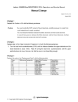
The extract syntax is written to the deck automatically along with the selected tests when the Write
Deck button on the Control popup is clicked on ( Figure 2-5:).
Figure 2-5: The ATLAS Extraction (Vt) Popup
SILVACO International
2-29
PC Interactive Tools User’s Manual
Extracted Results
Extracted results appear both with the simulator output in the tty subwindow and in a special file
named by default results.final. The file name can be user defined using the datafile="filename"
syntax. Use the file to compare the results from a large number of runs. For example, if using
DECKBUILD’s built-in optimizer, the file gives a concise listing of all the results as a function of the input
parameters. The extract results file is created in the current working directory.
Units
Material thickness (angstroms)
Junction depth (microns)
Impurity concentrations (impurity units, typically atoms/cm3)
Junction capacitance (Farads/cm2)
QUICMOS capacitance (Farads/cm2)
QUICKMOS 1D Vt (Volts)
QUICKBIP 1D solver (see the QUICKBIP section)
Sheet resistance (Ohm/square)
Sheet conductance (square/Ohm)
Electrode voltage (Volts)
Electrode internal voltage (Volts)
Electrode current (Amps)
Capacitance (Farads/micron)
Conductance (1/Ohms)
Transient time (Seconds)
Frequency (Hertz)
Temperature (Kelvin)
Luminescent power (Watts/micron)
Luminescent wavelength (Microns)
Available photo current (Amps/micron)
Source photo current (Amps/micron)
Optical wavelength (Microns)
Optical source frequency (Hertz)
Current gain (dB)
Unilateral power gain frequency (dB)
Max transducer power gain (dB)
The user can perform whatever unit shifting is required by adding the appropriate constants in the
device extract tests and saving them as the default, if desired. The units are always printed out along
with the extract results for built-in single value extract routines. Custom extract routines do not show
units.
2-30
SILVACO International
Extract Routines
Extract Features
Extract Name
Extract statements should almost always be given names. The name must be prepended to the
remainder of the extract statement. For example:
extract name="gateox thickness" oxide thickness x.val=1.0
The extract name is used in three ways. The name appears on the OPTIMIZER worksheet when the
extract statement is entered as a target, on the VWF worksheet as an extracted parameter, and can
also be used in further extract statements to perform variable substitution. The name can contain
spaces.
Variable Substitution
The extract parser maintains a list of variables, each of which consists of a name and a value. A name
is defined by any previous named extract statement. The corresponding value is the result of the
statement.
To refer to a variable’s value, precede it with a ‘$’. Quotes are optional around variable references,
except when the variable name contains spaces, in which case the $ must precede the quotes. The
substituted variable acts as a floating point number, and can be used in any extract expression that
uses numerical arguments.
For example:
extract name="xj1" xj silicon junc.occno=1
extract name="xj2" xj silicon junc.occno=2
extract name="deltaXj" abs($xj1 - $xj2)
Examples with spaces:
extract name="max boron" max.conc boron
extract name="max arsenic" max.conc arsenic
extract name="PN ratio" $"max boron"/$"max arsenic"
Variable substitution in extract can also be used with the set command as shown below:
set cutline=0.5
extract name="gateox thickness" oxide thickness x.val=$cutline
In addition, filenames to be loaded can also be specified this way, for example:
set efile = structure.str
extract init infile="$’efile’"
Note: Single quotes can be used to substitute where $-variable must appear within double quotes.
Min and Max Cutoff Values
Statements may contain min.val=value and/or max.val=value to define a valid range for extracted
results (single-valued results only; not curves). If either max or min is not defined, then the range
extends from +-infinity to the stated value, respectively. If the extracted value is outside the range,
then an error message is printed along with the extracted results and also appended to the default
results file.
SILVACO International
2-31
PC Interactive Tools User’s Manual
Multi-Line Extract Statements
Extract statements may be spread over multiple lines to specify layer biases and QSS values as shown
in above examples. This involves using the start/cont/done syntax.
Extraction and the Database (VWF)
When run with the VIRTUAL WAFER FAB, all extract values in the deck appear as output result columns
on the split worksheet. Each row of the worksheet contains the input parameters used to create the
results. The extracted value cell values are filled in automatically as the split points complete. If some
extracts are only intermediate calculations and are not required to be included in the results
worksheet the hide flag can be used. This prevents unrequired extract results from cluttering the
worksheet data.
The min/max extract ranges, if defined, are examined. If any extracted value is out of range, then
children of that deck fragment (any part of the worksheet that uses the simulation results of that deck
fragment) are automatically de-queued and marked with a parent error. The fragment is marked with
a range error. The purpose here is that the system does not waste its time by running any simulation
beyond that point in the input deck where the range error occurred, for all parts of the split tree that
use the particular values of the deck.
2-32
SILVACO International
Extract Routines
QUICKBIP Bipolar Extract
QUICKBIP is a 1D simulator for bipolar junction transistors (BJT), and is fully integrated inside the
DECKBUILD environment. It is accessed via the Extract command and is available for use with any
Silvaco simulator.
The doping profile passed to the QUICKBIP solver should be a bipolar profile. At least three regions
must exist. The top region in the first silicon layer is taken to be the emitter. There may be other
materials on top of the silicon.
QUICKBIP may be used with either ATHENA (2-D process simulation) or SSUPREM3 (1-D process
simulation). It is used in cases where a 1-D device simulation is both easier and faster to turn around
a result. Examples of the QUICKBIP extract command language are listed as follows:
extract
extract
extract
extract
extract
extract
extract
extract
extract
extract
extract
extract
extract
extract
extract
extract
extract
extract
extract
extract
extract
extract
name="bip
name="bip
name="bip
name="bip
name="bip
name="bip
name="bip
name="bip
name="bip
name="bip
name="bip
name="bip
name="bip
name="bip
name="bip
name="bip
name="bip
name="bip
name="bip
name="bip
name="bip
name="bip
test
test
test
test
test
test
test
test
test
test
test
test
test
test
test
test
test
test
test
test
test
test
bf" bf
nf" nf
is" gpis
ne" ne
ise" ise
cje" cje
vje" vje
mje" mje
rb" rb
rbm" rbm
irb" irb
tf" tf
cjc" cjc
vjc" vjc
mjc" mjc
ikf" ikf
ikr" ikr
nr" nr
br" br
isc" isc
nc" nc
tr" tr
Any name may be assigned to each command. In the case of a 2-D simulator the lateral position of the
vertical profile has to be specified with the parameter x.val=n, for example:
extract name = “forward transit time” tf x.val=0.3
Alternatively, a boolean region may be specified, when running in conjunction with the IC Layout
interface, for example:
extract name="my test" tf region="pnp_active_poly"
In this case, the bipolar test is performed only in the case where an IC layout cross section intersects
the named region.
QUICKBIP tuning parameters can also be modified for using the syntax shown below. A more detailed
explanation is provided in the Models and Algorithms section of Appendix A.
extract name="Tuning bf" bf x.val=0.5 bip.tn0=1.0e-5 bip.tp0=1.0e-3
bip.an0=2.9e-31 bip.ap0=0.98e-31 bip.nsrhn=5.0e12 bip.nsrhp=5.0e15
bip.betan=2.1 bip.betap=1.
SILVACO International
2-33
PC Interactive Tools User’s Manual
The extract parameters represent the BJT parameters given in Table 3-1:
Table 2-1: BJT Parameters
Parameter
Description
Units
bf
Ideal Maximum Forward Beta
nf
Forward current Emission Coefficient
gpis
Transport saturation current (IS)
ne
Base-Emitter Leakage Emission Coefficient
ise
Base-Emitter Leakage Saturation Current
A/cm2
cje
Base-Emitter Zero Bias DEpletion Capacitance
F/cm2
vje
Base-Emitter built in potential
V
mje
Base-Emitter exponential factor
rb
Zero bias base resistance
Ohms/square
rbm
Minimum base resistance at high current
Ohms/square
irb
Current at half base resistance value
A/cm2
tf
Ideal forward transit time (1/ft)
secs
cjc
Base-Collect zero bias depletion capacitance
F/cm2
vjc
Base-Collector built in potential
V
mjc
Base-Collector exponential factor
ikf
Corner of Forward Beta High current roll-off
A/cm2
ikr
Corner of Reverse Beta High current roll-off
A/cm2
nr
Reverse Current Emission Coefficient
br
Ideal Maximum Reverse Beta
isc
Base-Collector Leakage Saturation Current
nc
Base-Emitter Leakage Emission Coefficient
tr
Ideal forward transit time
A/cm2
A/cm2
secs
Automated command writing is accomplished with the use of the DeckBuild Extract popup window.
This is accessed from the Commands menu when either SSUPREM3 or ATHENA is selected as the
current simulator.
I-V Curves can be visualized with TONYPLOT if the Compute I-V curve option is selected on the
EXTRACT popup. In this case, select from either forward or reverse characteristics and specify the axes
of the curve.
•
All extracted parameters may be used as optimization targets.
•
All extracted parameters are appended to the default results file in the current working directory.
Unless specified using the datafile=filename syntax, it defaults to results.final.
2-34
SILVACO International
Extract Routines
•
When running under the VWF, all extracted parameters will be logged for regression modeling.
QUICKBIP solves fundamental system of semiconductor equations, continuity equations for electrons
and holes, and Poisson’s equation for potential self-consistently using the Gummel method. The
following physical models are taken into account by QUICKBIP:
•
Doping-dependent mobility
•
Electric field dependent mobility
•
Band gap narrowing
•
Shockley-Read-Hall recombination
•
Auger recombination
QUICKBIP is fully automatic so that it is unnecessary to specify input biases. QUICKBIP calculates
both forward and inverse characteristics of the BJT. For an n-p-n device, these sets are as follows:
1. Veb = -0.3... -Veb_final, Veb_step=-0.025, Vcb = 0 V
2. Vcb = -0.3... -Vcb_final, Vcb_step=-0.025, Veb = 0 V
3. Veb_final and Vcb_final depend on the particular BJT structures, usually about -1... -1.5(high
injection level).
For a p-n-p device, all signs are changed.
SILVACO International
2-35