1
LARSON•DAVIS
LABORATORIES
2900
User Manual
(5.xx Code)
Larson•Davis Laboratories
1681 W 820 N Provo, UT 84601
November 26, 1997
2900 Manual
Larson•Davis Incorporated
1681 West 820 North
Provo, Utah 84601
801-375-0177
Copyright
Copyright 1993 by Larson•Davis Incorporated. This manual and the hardware described in it are copyrighted, with all
rights reserved. The manual may not be copied in whole or in
part for any use without prior written consent of Larson•Davis Inc.
Trademarks
MS-DOS is a registered trademark of Microsoft Corp.
Warranty
Larson•Davis warrants this product to be free from defects in
material and workmanship for two years from the date of original purchase.
During the first year of the warranty period, Larson•Davis will
repair, or at its option, replace any defective component(s)
without charge for parts or labor. During the second year of the
warranty period, there will be no charge for replacement parts.
For customers within the continental United States, service is
provided for instruments returned, freight prepaid, to an authorized service center. The product will be returned freight prepaid.
For international customers, please contact your exclusive Larson•Davis representative for details on local service and shipping arrangements.
The Larson•Davis warranty applies only to products manufactured by Larson•Davis Inc., and does not include batteries.
Accessories and items not manufactured by Larson•Davis Inc.
are covered by the warranty of the original equipment manufacturer.
Product defects caused by misuse, accidents, or user modification are not covered by this warranty.
No other warranties are expressed or implied, Larson•Davis is
not responsible for consequential damages.
Larson•Davis Laboratories
TABLE OF CONTENTS
Chapter 1
Introduction.......................................................................................................1-1
Front Panel Controls .................................................................................................................... 1-2
Dedicated Hardkeys ................................................................................................................ 1-2
ASCII Hardkeys ....................................................................................................................... 1-3
Softkeys ................................................................................................................................... 1-4
The Arrow Keys and associated Hardkeys .................................................................................. 1-5
Cursor Control ......................................................................................................................... 1-5
Range Control.......................................................................................................................... 1-5
Instrument Boot-up Procedure ..................................................................................................... 1-6
Resetting RAM ............................................................................................................................. 1-7
Upgrading Software ..................................................................................................................... 1-7
Display Control............................................................................................................................. 1-7
Setting Backlight and Viewing Angle ....................................................................................... 1-7
Beeper Control ............................................................................................................................. 1-9
Color Monitor................................................................................................................................ 1-9
Power Supply ............................................................................................................................... 1-9
Battery Power .......................................................................................................................... 1-9
DC Power .............................................................................................................................. 1-10
Charging Batteries ................................................................................................................. 1-10
Microphone Connection ............................................................................................................. 1-10
Alternative Inputs ....................................................................................................................... 1-11
Accelerometers with Internal Electronics............................................................................... 1-11
Charge-coupled Accelerometers ........................................................................................... 1-11
Direct Voltage Inputs ............................................................................................................. 1-11
AC Outputs................................................................................................................................. 1-11
Single Channel Standard Analysis Mode .............................................................................. 1-11
Dual Channel Standard, Cross or Intensity Analysis Mode ................................................... 1-12
SLM Mode ............................................................................................................................. 1-12
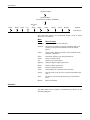
Front Panel Display Format ....................................................................................................... 1-12
Messages Displayed on the Left of the Screen ..................................................................... 1-12
Location A, Displayed Data Type ...................................................................................... 1-13
Location B, vsREF Display Status and Statistics .............................................................. 1-13
Location C, Autostore Status............................................................................................. 1-13
Location D, Frequency Trigger Status............................................................................... 1-13
Location E, Control Status................................................................................................. 1-14
Location F, Active File ....................................................................................................... 1-14
Messages Displayed on the Right of the Screen................................................................... 1-14
Note Display Line .............................................................................................................. 1-14
Location A, Units Name..................................................................................................... 1-14
Location B, Digital Differentiation or Integration and Bandwidth Compensation Status .... 1-14
Location C, Digital Display Weighting and Status of Time Trigger .................................... 1-15
Location D, Run Time........................................................................................................ 1-15
Location E, Averaging Type .............................................................................................. 1-15
Location F, Averaging Time............................................................................................... 1-15
Location G, Input Type ...................................................................................................... 1-16
1
2900 MANUAL
Location H, Analog Input Weighting .................................................................................. 1-16
Location I, Frequency Range between Highpass/Lowpass Filters with Linear Weighting Selected
1-16
Location J, Operational Status .......................................................................................... 1-16
Location K, Date and Time ................................................................................................ 1-16
Location L, Filter Status and Frequency at the Cursor Position ........................................ 1-16
Location M, Channel and Parameter Information.............................................................. 1-17
Location N, Amplitude Data corresponding to Cursor Position ......................................... 1-18
Location O, Loudness Level .............................................................................................. 1-19
Location P, Data from Tacho or Order Tracking Boards ................................................... 1-19
Location Q, Status of the Horizontal Arrow Keys .............................................................. 1-19
Noise Floor ............................................................................................................................ 1-20
Model 2800 and 2900 Specifications ......................................................................................... 1-21
Input....................................................................................................................................... 1-21
Analog Input Filters............................................................................................................ 1-21
Digital Characteristics ................................................................................................................ 1-21
Digitization ............................................................................................................................. 1-21
Anti-aliasing ........................................................................................................................... 1-21
Detector ................................................................................................................................. 1-21
Dynamic Range ..................................................................................................................... 1-22
Amplitude Stability ................................................................................................................. 1-22
Amplitude Linearity ................................................................................................................ 1-22
Filters ......................................................................................................................................... 1-22
Octave and Fractional Octave ............................................................................................... 1-22
FFT............................................................................................................................................. 1-22
Zoom Capability..................................................................................................................... 1-22
Time Domain Windows (FFT analysis).................................................................................. 1-23
Measured And Displayed Parameters ....................................................................................... 1-23
Sound Level Meter Mode (2800/2900) .................................................................................. 1-23
Standard Analysis Mode (2800/2900), Octave and FFT ....................................................... 1-23
Intensity Analysis Mode (2900 only), Octave and FFT .......................................................... 1-23
Cross Channel Analysis Mode (2900 only), FFT ................................................................... 1-23
Cross Channel Analysis Mode (2900 only, Octave Bandwidths............................................ 1-24
Digital Averaging ........................................................................................................................ 1-24
Octave Bandwidths................................................................................................................ 1-24
FFT Bandwidths..................................................................................................................... 1-24
Digital Display Weighting ........................................................................................................... 1-24
For Standard (2800/2900) and Intensity Analysis (2900 only) Modes;.................................. 1-24
Units ........................................................................................................................................... 1-25
Memory ...................................................................................................................................... 1-25
CMOS Non-volatile: ............................................................................................................... 1-25
Floppy Disk ............................................................................................................................ 1-25
Noise Generator......................................................................................................................... 1-25
Digital Output and Control.......................................................................................................... 1-25
Analog Outputs ...................................................................................................................... 1-26
Display Characteristics............................................................................................................... 1-26
Internal LCD........................................................................................................................... 1-26
External Color Display (Color Video Adapter required) ......................................................... 1-26
2
2900 MANUAL
Environmental ............................................................................................................................ 1-26
Physical...................................................................................................................................... 1-26
Power ......................................................................................................................................... 1-27
Battery Power ........................................................................................................................ 1-27
DC Power .............................................................................................................................. 1-27
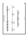
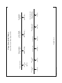
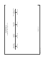
2900 Block Diagram................................................................................................................... 1-28
Chapter 2
Menu Structure For Instrument Operation .....................................................2-1
Softkey Menu Concept................................................................................................................. 2-1
Analyzer Mode......................................................................................................................... 2-1
Submenus................................................................................................................................ 2-2
Sound Level Meter Modes ........................................................................................................... 2-3
Shift Menu .................................................................................................................................... 2-4
Chapter 3
Sound Level Meter Operating Modes .............................................................3-1
Sound Pressure Level Measurements: Single Channel Sound Level Meter with Frequency Analysis
(SLM+A) Mode............................................................................................................................. 3-2
Setup ....................................................................................................................................... 3-2
Changing the Microphone Bias Voltage .................................................................................. 3-3
Changing the Microphone Input............................................................................................... 3-3
Changing the SLM Analog Filters ............................................................................................ 3-4
Selecting SLM and Frequency Analysis Weighting ................................................................. 3-4
Warm-up Time ......................................................................................................................... 3-5
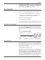
Alignment of the Microphone Boom and Microphone/Preamplifier .............................................. 3-5
Microphone Boom Alignment................................................................................................... 3-5
SLM Standards ........................................................................................................................ 3-6
IEC 651-1979........................................................................................................................... 3-6
ANSI S1.4-1983....................................................................................................................... 3-6
Microphone/Preamplifier Alignment......................................................................................... 3-6
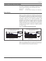
Free-Field Measurements........................................................................................................ 3-7
Random Incidence Measurements .......................................................................................... 3-9
Effect of Windscreen.............................................................................................................. 3-10
Position of Operator............................................................................................................... 3-11
Making a Sound Level Measurement .................................................................................... 3-11
Adjusting the Input Gain ........................................................................................................ 3-11
Overload Indication................................................................................................................ 3-12
Autoranging ........................................................................................................................... 3-12
Measurement Range ............................................................................................................. 3-12
Primary Indicator Range ........................................................................................................ 3-14
Non-linear Distortion .............................................................................................................. 3-14
Selecting the Displayed Parameter............................................................................................ 3-14
Frequency Analysis Display ....................................................................................................... 3-16
Calibration .................................................................................................................................. 3-17
Sound Level Calibrator .......................................................................................................... 3-17
Calibration Procedure ............................................................................................................ 3-17
Effect of Microphone Extension Cable................................................................................... 3-19
Noise Floor Measurement and Proximity Message ................................................................... 3-19
3
2900 MANUAL
Environmental Effects on SLM Measurements .......................................................................... 3-20
Magnetic Field ....................................................................................................................... 3-20
Temperature .......................................................................................................................... 3-20
Humidity................................................................................................................................. 3-20
Temperature and Humidity; Permanent Damage .................................................................. 3-21
Effect of Vibration .................................................................................................................. 3-21
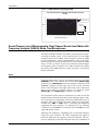
Sound Pressure Level Measurements; Dual Channel Sound Level Meter with Frequency Analysis
(SLM+A) Mode, Two Microphones ............................................................................................ 3-22
Setup ..................................................................................................................................... 3-22
Sound Pressure Level Measurement; Dual Channel Sound Level Meter with Frequency Analysis
(SLM+A), Single Microphone ..................................................................................................... 3-23
Sound Pressure Level Measurements using the Wide Dynamic Range Sound Level Meter (WDR
SLM) function ............................................................................................................................. 3-23
Accessing the WRD SLM Menu ............................................................................................ 3-23
Selecting the Microphone Input and the Bias Voltage ........................................................... 3-24
Selecting the Frequency Weighting ....................................................................................... 3-25
Chapter 4
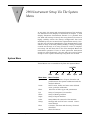
2900 Instrument Setup Via The System Menu ...............................................4-1
System Menu ............................................................................................................................... 4-1
Accessing the System Menu ................................................................................................... 4-2
Selection of Analysis Type....................................................................................................... 4-2
Standard Mode .................................................................................................................... 4-2
Cross Mode ......................................................................................................................... 4-3
Intensity Mode ..................................................................................................................... 4-3
Frequency Range Considerations ........................................................................................... 4-3
Octave Frequency Analysis................................................................................................. 4-3
FFT Frequency Analysis...................................................................................................... 4-3
Selection of Filter Type ............................................................................................................ 4-4
Accessing the Filter Menu ................................................................................................... 4-4
Selection of Octave and Fractional Octave Filters .............................................................. 4-5
Selection of FFT Filtering .................................................................................................... 4-6
Selection of Number of Lines .............................................................................................. 4-7
Selection of Time Weighting Window .................................................................................. 4-7
Selection of Baseband Full Scale Frequency (Base-Bd)..................................................... 4-9
FFT Zoom Analysis to Increase Frequency Resolution....................................................... 4-9
Limitation on Zoom Multiplier............................................................................................. 4-11
Printing FFT Data in Tabular Format................................................................................. 4-12
Accessing Input Menu ........................................................................................................... 4-12
Setting the Microphone Bias Voltage ................................................................................ 4-12
Branching a Signal from One Input Connector to both Analysis Channels (Dual Channel Analysis
Only, Standard or Sound Level Meter)....................................................................................... 4-13
Setting the Analog Filters for the Frequency Analysis Function ........................................ 4-13
Internal Calibration Signal...................................................................................................... 4-13
Offsetting Gain Between Channels ................................................................................... 4-14
Setting the Autorange Aperture ......................................................................................... 4-14
Operation of the Noise Generator (OPT 10 Required) .......................................................... 4-14
Connection ........................................................................................................................ 4-15
Selecting Spectral Content ................................................................................................ 4-15
Selecting Operational Mode .............................................................................................. 4-15
Operation of the Signal Generator (OPT 11 Required) ......................................................... 4-16
Operational Mode .............................................................................................................. 4-16
4
2900 MANUAL
Sine Generator, Single Tone ............................................................................................. 4-16
Sine Generator, Dual Tone................................................................................................ 4-18
Autolevel Control; Sine Generator..................................................................................... 4-19
Pink Noise Generator; Wideband or Bandlimited .............................................................. 4-20
Autolevel Control; Bandlimited Pink Noise ........................................................................ 4-21
White Noise Generator; Wideband or Pseudo .................................................................. 4-22
Pulse Generator ................................................................................................................ 4-22
Interface Operations .............................................................................................................. 4-23
Selection of Intensity Probe or Remote Control..................................................................... 4-23
Remote Control using Model 3200RC Remote Control Module ............................................ 4-24
Setup ................................................................................................................................. 4-24
Operation........................................................................................................................... 4-25
Communication with User-defined Setups ........................................................................ 4-25
DC Output.............................................................................................................................. 4-26
I/O Port Control...................................................................................................................... 4-27
A/D Inputs #1, #2 and #3................................................................................................... 4-27
I/O Channels #1, #2 and #3................................................................................................... 4-27
Frequency Domain Interface Trigger of I/O Channel 3.......................................................... 4-28
Key A and Key B Control ....................................................................................................... 4-29
Beeper Control....................................................................................................................... 4-30
Selecting the RS-232 Interface.............................................................................................. 4-30
Setting the Clock.................................................................................................................... 4-30
The Resets Menu .................................................................................................................. 4-31
Remaining System Softkeys.................................................................................................. 4-32
Chapter 5
Selection of Averaging Parameters ................................................................5-1
Selecting Averaging Type ............................................................................................................ 5-1
Accessing Averaging Menu ..................................................................................................... 5-1
Averaging Type: Octave Filters ............................................................................................... 5-1
Averaging Type: FFT Filters .................................................................................................... 5-2
Averaging Time ............................................................................................................................ 5-3
Averaging Time with Linear Types .......................................................................................... 5-3
Averaging Time with Exponential Types.................................................................................. 5-3
Averaging Time with Constant Confidence Type (Octave Bandwidths Only).......................... 5-4
Averaging Time with Spectral Type Averaging (FFT Bandwidths Only).................................. 5-4
Signal Averaging Considerations ................................................................................................. 5-5
Stationary Signals.................................................................................................................... 5-5
Time Averaging ................................................................................................................... 5-5
Linear Time Averaging ........................................................................................................ 5-6
Constant Confidence Time Averaging................................................................................. 5-6
Spectrum Averaging ............................................................................................................ 5-6
Periodic Signals................................................................................................................... 5-7
Transient Signals ..................................................................................................................... 5-7
Linear Repeat Time Averaging............................................................................................ 5-7
Exponential Time Averaging................................................................................................ 5-7
Chapter 6
Analysis Menus; Selection Of Measurement And Display Parameters.......6-1
Standard Analysis ........................................................................................................................ 6-1
Selection of Display Format for Dual Channel Mode............................................................... 6-2
Average Spectrum Display ...................................................................................................... 6-2
5
2900 MANUAL
Selection of Display Parameter ............................................................................................... 6-3
Max Spectrum Display............................................................................................................. 6-3
Dual Channel Display Mode .................................................................................................... 6-4
Loudness Measurement .......................................................................................................... 6-5
Cross Analysis ............................................................................................................................. 6-6
Cross Analysis of FFT Filters................................................................................................... 6-6
Selection and Indication of Displayed Channel ................................................................... 6-8
Display of Complex Data Records:...................................................................................... 6-8
Display of Time Records ..................................................................................................... 6-9
Cross Analysis with Octave Filters .......................................................................................... 6-9
Intensity Analysis ....................................................................................................................... 6-10
Display of Broadband Data ........................................................................................................ 6-10
Chapter 7
Performing a Measurement .............................................................................7-1
Manual Control of Run/Stop......................................................................................................... 7-1
Continuously Running Time Averaging ................................................................................... 7-1
Finite Length Time Averaging.................................................................................................. 7-2
Input Gain Control ........................................................................................................................ 7-2
Manual Control of Input Gain................................................................................................... 7-2
Offsetting Gain Between Channels.......................................................................................... 7-3
Autorange of Input Gain........................................................................................................... 7-3
Response Time of Digital Filters .................................................................................................. 7-4
Possible Overload Indication upon Resuming Analysis........................................................... 7-4
Chapter 8
Cursor Control ..................................................................................................8-1
Solid and Dotted Cursors Moving Independently......................................................................... 8-1
Solid and Dotted Cursors Moving Together ................................................................................. 8-2
Harmonic Cursors ........................................................................................................................ 8-2
Fixing Cursor Positions ................................................................................................................ 8-3
Chapter 9
Selection of Units and Calibration ..................................................................9-1
Units ............................................................................................................................................. 9-1
Accessing Units Menu ............................................................................................................. 9-1
Creation of Unit Names ........................................................................................................... 9-1
Assignment of Unit Names ...................................................................................................... 9-2
Assignment of Integration or Differentiation............................................................................. 9-2
1/1 and 1/3 Octave Integration and Differentiation Operations................................................ 9-3
FFT Integration and Differentiation Operations ....................................................................... 9-3
Calibration .................................................................................................................................... 9-4
Calibration Based on a Transducer Sensitivity Value.............................................................. 9-4
Logarithmic Units Calibration (dB⁄Volt) ................................................................................ 9-4
Logarithmic Units Calibration Microphone K-factor ............................................................. 9-5
Linear Units Calibration ....................................................................................................... 9-5
Calibration Based on a Reference Signal................................................................................ 9-6
Calibration Using the Test Signal ............................................................................................ 9-7
Storage and Recall of Units Information ...................................................................................... 9-7
Storage of Units Data .............................................................................................................. 9-8
Recall of Units Data ................................................................................................................. 9-8
6
2900 MANUAL
Chapter 10 Digital Display including Broadband Acoustic Frequency Weighting, User-defined Frequency Weighting and Integration of FFT Spectra..............10-1
Accessing the Display Menu ...................................................................................................... 10-1
Selecting Bandwidth for Display of 1/3 Octaves .................................................................... 10-2
Display of the Average Spectrum .......................................................................................... 10-2
Selecting Integration .............................................................................................................. 10-2
Digital Display Weighting ........................................................................................................... 10-3
Accessing the Digital Weighting Menu .................................................................................. 10-3
Exiting From Display Weighting............................................................................................. 10-4
User Weighting........................................................................................................................... 10-4
Creating a User Weighting Curve .......................................................................................... 10-5
Interpolation Function ............................................................................................................ 10-5
Creating a User Weighting Curve from a Measured Spectrum ............................................. 10-5
The Active Register ............................................................................................................... 10-6
Storing the Active Register into Storage Registers................................................................ 10-6
Recalling from Storage Registers .......................................................................................... 10-7
Adding Registers ................................................................................................................... 10-7
Subtracting Registers ............................................................................................................ 10-7
Storage of User Curve Records............................................................................................. 10-7
Recall of User Curves............................................................................................................ 10-8
Exiting from the Setuser Menu .............................................................................................. 10-8
Chapter 11 Trigger Functions ...........................................................................................11-1
Time-domain Triggering ............................................................................................................. 11-1
Trigger Level.......................................................................................................................... 11-1
Trigger Slope ......................................................................................................................... 11-2
Trigger Delay ......................................................................................................................... 11-2
Channel 2 Delay .................................................................................................................... 11-4
Arming and Disabling............................................................................................................. 11-4
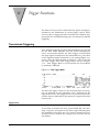
Frequency Domain Triggering.................................................................................................... 11-4
Selecting Trigger Frequency.................................................................................................. 11-5
Selecting the Trigger Criterion ............................................................................................... 11-5
Selecting the Trigger Level .................................................................................................... 11-6
Frequency Domain Trigger Setup for the SLM Mode ............................................................ 11-6
Arming and Disabling............................................................................................................. 11-6
Automatic Re-Arming............................................................................................................. 11-7
Chapter 12 Storage and Recall of Instrument Setups ....................................................12-1
Labeling and Assigning Softkeys ............................................................................................... 12-2
Changing 2900 Setup from Softkeys ..................................................................................... 12-2
Reset of User-defined Setups................................................................................................ 12-2
Storage of User-defined Setups ............................................................................................ 12-2
Recall of User-defined Setups ............................................................................................... 12-3
Exiting from the Setup Menu ................................................................................................. 12-3
Chapter 13 Storing and Recalling Non-Autostore Data..................................................13-1
Files Operations ......................................................................................................................... 13-1
7
2900 MANUAL
Accessing the Files Menu...................................................................................................... 13-1
Files Information .................................................................................................................... 13-1
Creation of Files..................................................................................................................... 13-2
Renaming Files...................................................................................................................... 13-2
Deleting Files ......................................................................................................................... 13-3
Formatting a Floppy Disk....................................................................................................... 13-3
File Transfers to/from Disk..................................................................................................... 13-3
Selection of the Active File .................................................................................................... 13-4
Record Operations from the Files Menu .................................................................................... 13-4
Classification of Record Types .............................................................................................. 13-4
Records Listing ...................................................................................................................... 13-5
Note Editing ........................................................................................................................... 13-5
Deleting Records ................................................................................................................... 13-5
Recalling a Record from the Files Menu................................................................................ 13-5
Storage of Normal (Non-autostored) Data to Internal Memory .................................................. 13-6
Storage of Data Blocks .......................................................................................................... 13-6
Record Classification ............................................................................................................. 13-6
Storage Verification ............................................................................................................... 13-9
Setup Information .................................................................................................................. 13-9
Notes ..................................................................................................................................... 13-9
Recall and Display of Data Records (Non-autostored) from Memory ........................................ 13-9
Analyzer Setup for Recall .................................................................................................... 13-10
Recall Operation .................................................................................................................. 13-10
Record Type and Number Indication ................................................................................... 13-11
Note Presentation ................................................................................................................ 13-11
Changing Displayed Record Number .................................................................................. 13-11
Cursor Utilization ................................................................................................................. 13-11
Deleting Stored Records .......................................................................................................... 13-12
Block Averaging of Stored Records ......................................................................................... 13-12
Block Maximum of Stored Records.......................................................................................... 13-12
Block Summation of Stored Records ....................................................................................... 13-13
Waterfall Display of Stored Records ........................................................................................ 13-14
Exiting from the Recall Mode............................................................................................... 13-15
Memory Requirements (Non-autostore Records) .................................................................... 13-16
Chapter 14 Annotation of Data Blocks.............................................................................14-1
Annotation of Data Blocks.......................................................................................................... 14-1
Chapter 15 Autostore by Time ..........................................................................................15-1
Setup for an Autostore Sequence .............................................................................................. 15-1
Accessing the Autostore Menu .............................................................................................. 15-1
Defining Delta Time and End Time........................................................................................ 15-2
Delta Time Limitations ........................................................................................................... 15-2
Selection of Spectral Type to be Autostored ......................................................................... 15-3
Count Averaging Special Considerations .............................................................................. 15-3
Initiation of an Autostore byTime Sequence .............................................................................. 15-3
8
2900 MANUAL
Manual Start .......................................................................................................................... 15-3
Frequency Trigger Start......................................................................................................... 15-4
Conclusion of an Autostore byTime Sequence .......................................................................... 15-5
Disabling Autostore byTime................................................................................................... 15-5
Data Storage Format.................................................................................................................. 15-6
Averaging Time Considerations ................................................................................................. 15-6
FFT Analysis.......................................................................................................................... 15-6
Octave Filters......................................................................................................................... 15-7
Recall and Display of Autostored Data ...................................................................................... 15-7
Displaying Individual Spectra................................................................................................. 15-8
Cursor Control ....................................................................................................................... 15-9
Display of Amplitude vs. Time.................................................................................................... 15-9
Leq Measurements in the vsTime Display Mode................................................................. 15-10
Changing the Displayed Frequency Band ........................................................................... 15-11
Broadband Level versus Time ............................................................................................. 15-11
SLM Data versus Time ........................................................................................................ 15-11
Displaying the Same Frequency of Another Record............................................................ 15-12
Displaying and Storing Leq, MIN, MAX, SEL, and Mx.Spec Spectra....................................... 15-12
Deleting Autostore Records ..................................................................................................... 15-13
Averaging of Autostore byTime Records ................................................................................. 15-13
Block Maximum of Autostored byTime Records ...................................................................... 15-14
Block Summation of Autostored byTime Records.................................................................... 15-15
Waterfall Display of Autostored Records ................................................................................. 15-16
Chapter 16 Autostore by Tach ..........................................................................................16-1
Tachometer Input (TACH).......................................................................................................... 16-1
Second Tachometer Input (SPEED) .......................................................................................... 16-1
TACH/SPEED Display in Intensity Mode ................................................................................... 16-1
byTach Autostore ....................................................................................................................... 16-2
Setting the Tacho Parameters ................................................................................................... 16-2
Tach/Speed Scaling............................................................................................................... 16-3
Interval and Span Settings..................................................................................................... 16-4
Influence of Slope on Test Procedure ................................................................................... 16-6
Tach/Speed Calibration ......................................................................................................... 16-7
Trigger Smoothing ................................................................................................................. 16-8
Enabling Autostore byTach ........................................................................................................ 16-9
Recall of Data Autostored byTach ........................................................................................... 16-10
Displaying Individual Spectra............................................................................................... 16-11
Channel Selection................................................................................................................ 16-11
Cursor Control ..................................................................................................................... 16-11
Averaging of Autostore byTach Records ................................................................................. 16-11
Block Maximum of Autostored byTach Records ...................................................................... 16-13
Waterfall Display of Autostored Records ................................................................................. 16-14
vsRPM Graphics ...................................................................................................................... 16-15
9
2900 MANUAL
Chapter 17 vsRPM Graphics .............................................................................................17-1
Real-time vsRPM Graphics........................................................................................................ 17-2
Color Monitor Pen Format ..................................................................................................... 17-2
LCD Display Pen Format ....................................................................................................... 17-3
Accessing a Trace ................................................................................................................. 17-4
Pen Selection......................................................................................................................... 17-4
Channel Selection.................................................................................................................. 17-4
Frequency Band Selection..................................................................................................... 17-4
Order Selection...................................................................................................................... 17-5
RPM/Speed Selection............................................................................................................ 17-5
Horizontal Scale Selection..................................................................................................... 17-5
Slope Selection...................................................................................................................... 17-5
Incremental Control of the Trace ........................................................................................... 17-6
Control of Trace Status.......................................................................................................... 17-7
Suspending Color Monitor Updates....................................................................................... 17-7
Performing a Test .................................................................................................................. 17-7
Examination of the Traces ..................................................................................................... 17-8
Hiding Traces......................................................................................................................... 17-8
Storage of Trace Displays ..................................................................................................... 17-8
Recall of Trace Displays ........................................................................................................ 17-8
vsRPM Graphics from byTach Autostored Records .................................................................. 17-9
Standard Mode Data.............................................................................................................. 17-9
Modification of the Graphic Parameters ................................................................................ 17-9
Storage and Recall of Trace Records.................................................................................. 17-10
Intensity Mode Data............................................................................................................. 17-10
Post-process Order Tracking ................................................................................................... 17-11
Peak Hunt Procedure .......................................................................................................... 17-12
Bandwidth Averaging Procedure ......................................................................................... 17-13
Chapter 18 Statistics and Ln Calculations.......................................................................18-1
Setup for Statistical Analysis...................................................................................................... 18-1
Setting the Update Interval .................................................................................................... 18-2
Setting Measurement Range ................................................................................................. 18-2
Use of Autoranging ................................................................................................................ 18-2
Turning the Statistics Analysis On and Off ............................................................................ 18-3
Selecting the Ln Values for Calculation and Display ............................................................. 18-3
Running the Statistics Mode .................................................................................................. 18-4
Calculation and Display of Data............................................................................................. 18-4
Selecting the Display Channel Number ................................................................................. 18-5
Modifying the Parameter Table Values.................................................................................. 18-5
Hiding a Trace ....................................................................................................................... 18-5
Clearing the Statistics Table .................................................................................................. 18-6
Storing the Ln Trace .............................................................................................................. 18-6
Storing the Statistics Table .................................................................................................... 18-6
Recalling Ln Traces ............................................................................................................... 18-6
Recalling a Statistics Table.................................................................................................... 18-7
10
2900 MANUAL
Merging Statistics Tables....................................................................................................... 18-7
Chapter 19 ControlofDisplayFormats,Cross-ChannelNormalizationandUseofKeyMacros
19-1
Accessing the Display Menu ...................................................................................................... 19-1
Dual Channel Side-by-Side Display Mode ................................................................................. 19-1
Displaying 1/3 Octave Spectra in 1/1 Octave Format ................................................................ 19-2
Digital Reading of A-Weight and Summation Bands.................................................................. 19-2
Digital Display Weighting ........................................................................................................... 19-2
Display of Spectra Relative to a Reference Spectrum ............................................................... 19-3
Dual Channel Measurements ................................................................................................ 19-4
Returning to Normal Display Format ..................................................................................... 19-4
Control of Vertical Display.......................................................................................................... 19-4
Control of Display Range....................................................................................................... 19-5
Bandwidth Compensation (Power Spectral Density) ................................................................. 19-7
Control of Horizontal Display...................................................................................................... 19-8
Selection of Logarithmic/Linear Format ................................................................................. 19-8
Control of Display Range....................................................................................................... 19-8
Normalization of Amplitude and Phase Between Channel 1 and Other Channels .................... 19-9
Connection of the Noise Generator............................................................................................ 19-9
Normalization in Cross Mode, Using FFT Filtering .................................................................. 19-10
Selection of 100 Line Resolution ......................................................................................... 19-10
Selection of Baseband Full Scale Frequency ...................................................................... 19-10
Noise Generator Setup ........................................................................................................ 19-10
Measurement....................................................................................................................... 19-10
Normalization....................................................................................................................... 19-11
Toggling Normalization ON and OFF .................................................................................. 19-11
Normalization in the Cross Mode, using Octave Bandwidths .................................................. 19-12
Key Macros .............................................................................................................................. 19-12
Creating Macros .................................................................................................................. 19-12
McSTOP and McWAIT and McREPT Softkeys ................................................................... 19-13
Resetting Macros................................................................................................................. 19-13
Executing Macros ................................................................................................................ 19-13
Delayed Macro Execution.................................................................................................... 19-14
Storing Macros..................................................................................................................... 19-14
Recalling Macros ................................................................................................................. 19-14
Chapter 20 Sound Intensity Measurements.....................................................................20-1
Sound Intensity Standards ......................................................................................................... 20-2
Instrument Standards ............................................................................................................ 20-2
Application Standards............................................................................................................ 20-3
Setup and Calibration of the Measurement System................................................................... 20-3
Sound Pressure Level Calibration ......................................................................................... 20-3
Setup for 1/3 octave Intensity Measurement ......................................................................... 20-3
Pressure, Temperature and Spacer Length Input ................................................................. 20-4
Amplitude and Phase Normalization; 1/1, 1/3 Octave Measurements .................................. 20-4
11
2900 MANUAL
Sound Intensity using Narrow Band (FFT) Analysis .................................................................. 20-7
Definition of Surface Area (m2) for the Power Calculation......................................................... 20-7
Job, Part, Area Labels................................................................................................................ 20-8
Entering Label Names ......................................................................................................... 20-10
Selection of Display Parameters .............................................................................................. 20-11
Selecting Displayed Parameters.......................................................................................... 20-11
Readout of Broadband Levels ............................................................................................. 20-11
Reducing the Frequency Display Range ............................................................................. 20-11
Reducing the Amplitude Display Range .............................................................................. 20-12
Performing the Intensity Measurement .................................................................................... 20-12
Storage and Recall of Intensity Spectra................................................................................... 20-13
Editing the JOB, PART and AREA Names, the surface Area value and the Note Field of a Stored
Intensity Spectrum ............................................................................................................... 20-14
Power Summation.................................................................................................................... 20-15
Accessing Power Summation Menu .................................................................................... 20-15
Search Field Concept .......................................................................................................... 20-15
Manually Entering Labels into the Search Field .................................................................. 20-16
Entering Labels by Recalling Spectra.................................................................................. 20-16
Performing a Power Summation.......................................................................................... 20-16
Storage of Power Spectra.................................................................................................... 20-17
Recall of Power Spectra ...................................................................................................... 20-17
Power Summation Example ................................................................................................ 20-17
Three Level Search: ........................................................................................................ 20-18
Two Level Search:........................................................................................................... 20-18
Single Level Search:........................................................................................................ 20-18
Field Indicators Specified in the Standard ISO 9614-1: 1993 (E) ............................................ 20-19
Temporal Variability Indicator (F1)....................................................................................... 20-19
Surface Pressure-intensity Indicator (F2), Negative Partial Power Indicator (F3), and Field
Non-uniformity Indicator (F4) ............................................................................................... 20-20
Surface Pressure—Intensity Indicator ............................................................................. 20-20
Negative Partial Power Indicator ..................................................................................... 20-21
Field Non-Uniformity Indicator ......................................................................................... 20-21
Alternate Presentation Format for F2, F3 and F4 ................................................................ 20-23
Chapter 21 Room Acoustics Measurements ...................................................................21-1
Sound Decay Measurements..................................................................................................... 21-1
Use of the Noise Generator ................................................................................................... 21-2
Procedure .......................................................................................................................... 21-2
Use with Impulsive Excitation ................................................................................................ 21-3
Evaluation of Reverberation Time.............................................................................................. 21-4
RT60 Register........................................................................................................................ 21-4
Reading Current RT60........................................................................................................... 21-5
Manual Entry of RT60 Values................................................................................................ 21-5
Manual Determination of RT60 Using the Cursors ................................................................ 21-6
Automatic Determination of RT60 Using Max–based Thresholds ......................................... 21-7
Automatic Determination of RT60 Using Fixed Thresholds................................................. 21-10
Averaging of Autostored Time Decay Records.................................................................... 21-11
Storage and Recall of RT60 Data ............................................................................................ 21-12
12
2900 MANUAL
Recall of RT60 ..................................................................................................................... 21-12
Room Acoustics Measurements .............................................................................................. 21-12
Airborne Sound Transmission Loss Measurements ............................................................ 21-13
ASTM Airborne Sound Transmission Parameters............................................................... 21-15
ISO Airborne Sound Transmission Parameter .................................................................... 21-16
Impact Sound Insulation Measurements ............................................................................. 21-18
ASTM Impact Sound Transmission ..................................................................................... 21-19
ISO Impact Isolation ............................................................................................................ 21-20
Noise Criteria Curves........................................................................................................... 21-21
Noise Rating Curves............................................................................................................ 21-22
The RC Noise Rating Procedure ......................................................................................... 21-22
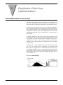
Chapter 22 Classification (Class) Lines (Optional Feature) ...........................................22-1
General Explanation of the Concept .......................................................................................... 22-1
Accessing the Class Lines..................................................................................................... 22-3
Labeling the Class Lines........................................................................................................ 22-4
Creating a Single Class Line ................................................................................................. 22-4
Assigning Max or Min Mode .................................................................................................. 22-7
Creating Multiple Class Lines ................................................................................................ 22-8
Turning On a Class Line Family ............................................................................................ 22-8
Assigning Class Lines to an Input Channel ........................................................................... 22-8
Automatic Judgement of Spectra (all channels) Using a Softkey .......................................... 22-9
Manual Judgement of a Displayed Spectrum using a Softkey ............................................ 22-10
Automatic Judgement Based on Stop State of Analyzer ..................................................... 22-11
Classifications Requiring Line Crossings at Multiple Frequencies ...................................... 22-11
Storage of Class Lines to Setup Menu Softkeys ................................................................. 22-12
Recalling a Set of Class Lines from Setup Menu Softkeys.................................................. 22-12
Storing Class Lines Stored under Setup Menu Softkeys to Non–volatile Memory .............. 22-13
Recalling Class Lines from Non–Volatile Memory to the Class Lines Setup Softkeys ........ 22-13
Turning Off the Class Lines Function .................................................................................. 22-13
Chapter 23 2900 Printing Data Screen Displays and Tables..........................................23-1
Accessing the Print Menu .......................................................................................................... 23-1
Initializing the Printer.................................................................................................................. 23-1
Creating the Logo....................................................................................................................... 23-1
Selecting Printer Type................................................................................................................ 23-2
Printing the LCD Screen Display................................................................................................ 23-2
Printing a Data Table ................................................................................................................. 23-2
Printing LCD Screen Display and Data Table ............................................................................ 23-2
Print to Screen (List) Function.................................................................................................... 23-2
Aborting a Printout ..................................................................................................................... 23-3
Ejecting a Sheet of Paper, or Making a Form Feed ................................................................... 23-3
Printing the Color Monitor Display.............................................................................................. 23-3
Block Printing of Stored Data Records....................................................................................... 23-3
Custom Printouts........................................................................................................................ 23-4
Accessing the Custom Printout Module................................................................................. 23-4
13
2900 MANUAL
Scaling of the Custom Printout .............................................................................................. 23-4
General Description ............................................................................................................... 23-8
Custom Graphic Configuration .............................................................................................. 23-9
LCD Graphic Printout........................................................................................................... 23-10
Measurement Parameter Text Strings................................................................................. 23-10
User Text Strings ................................................................................................................. 23-11
Storing a Custom Printout Setup to a Softkey ..................................................................... 23-11
Recalling a Custom Print Setup from a Softkey................................................................... 23-12
Storing Print Setups to Memory........................................................................................... 23-12
Recalling Print Setups from Memory ................................................................................... 23-13
Default Custom Printout Setups .......................................................................................... 23-13
Initiating Printing of a Custom Printout ................................................................................ 23-15
Chapter 24 Use of External Color Monitor for Display and Instrument Control...........24-1
Hardware Considerations........................................................................................................... 24-1
Activating the External Monitor .................................................................................................. 24-3
System Operation Using Pop-Up Control Window..................................................................... 24-4
Selecting the Number of Display Windows............................................................................ 24-5
System Operation Without the Control Window......................................................................... 24-5
Global Configuration Windows .............................................................................................. 24-5
Base Frequency..................................................................................................................... 24-5
Selection of Analysis Type..................................................................................................... 24-6
Selection of Filter Type .......................................................................................................... 24-6
Selection of Detector Type .................................................................................................... 24-6
Selection of Averaging Time.................................................................................................. 24-6
Selection of Master Display Type .......................................................................................... 24-7
Selecting the Number of Analysis Channels.......................................................................... 24-8
Selecting the Number of Data Display Windows ................................................................... 24-8
Setting the Range (Input Gain) .............................................................................................. 24-8
Selecting vsTime or vsTach Autostore .................................................................................. 24-9
Running and Stopping the Analysis....................................................................................... 24-9
Individual Data Display Windows........................................................................................... 24-9
Display Type .......................................................................................................................... 24-9
Channel Number.................................................................................................................. 24-10
Selection of Broadband and Highpass/lowpass Filters........................................................ 24-10
Selection of Units................................................................................................................. 24-10
Cursor Control and Selection of Graphic Display Parameters ................................................. 24-11
Cursor Control ..................................................................................................................... 24-11
Vertical Display Range Control............................................................................................ 24-11
Horizontal Display Range Control........................................................................................ 24-11
Line Type ............................................................................................................................. 24-12
Linear and A-Weighted Data ............................................................................................... 24-12
Recall and Display of Data....................................................................................................... 24-13
Running Macros................................................................................................................... 24-13
Recalling Setups.................................................................................................................. 24-13
Displaying in the vsRPM/Speed Format .................................................................................. 24-14
14
2900 MANUAL
Selecting the vsRPM/Speed Format.................................................................................... 24-14
Selecting vsRPM or vsSpeed .............................................................................................. 24-15
Assigning Pens to Frequencies or Orders ........................................................................... 24-15
Assigning Traces to Pens .................................................................................................... 24-16
Hiding or Unhiding Traces ................................................................................................... 24-16
Cursor Control ..................................................................................................................... 24-16
Modifying the Left and Right RPM/Speed Axis Limit ........................................................... 24-16
Selecting Band Tracking...................................................................................................... 24-17
Chapter 25 Softkey Menus ................................................................................................25-1
Appendix A Index ................................................................................................................. A-1
15
2900 MANUAL
16
1
Introduction
The Model 2900 Real-time SLM performs two measurement
functions simultaneously; that of a Precision Sound Level
Meter and that of a real-time frequency analyzer.
As a digital sound level meter, it simultaneously calculates
the sound pressure level corresponding to the following
detectors: RMS Slow, RMS Fast, Impulse and Peak. The Min
and Max values of the Slow, Fast and Impulse detectors over
the measurement period are maintained. At the same time, it
calculates both LEQ and SEL integrated values. In certain
versions of the Model 2900, such as delivered to German
users, the Min and Max values of the Impulse weighted
sound level are replaced by the Taktmaximal (Fast weighted)
3 and 5 values.
As a real-time analyzer, it can perform single or dual channel
frequency analysis using digital 1/1 and 1/3 octave bandwidths and FFT analysis using 100, 200, 400 or 800 line resolution. When equipped with the optional OPT 80 Acoustic
Intensity Module, and using a Larson•Davis intensity probe,
it can perform acoustic intensity measurements in both digital (1/1 and 1/3 octave) and FFT filter formats. Using digital
filters, it can generate statistics and Ln data using one or two
channels.
In its autostore mode, it can store spectra as fast as 400
spectra/second to non-volatile memory, and subsequently
display data in selected bandwidths as a function of time.
Additional on-board software permits the calculation and display of reverberation time, sound transmission loss, NC, and
STC. Along with these analysis capabilities, the 2900 provides a high degree of versatility in data presentation on the
screen. The user may control the vertical and horizontal
screen formats (log/linear) as well as the display ranges. In
conjunction with horizontal and vertical display expansion
capabilities to provide the highest visual resolution of data,
vertical window and horizontal pan functions may be used to
move the expanded data blocks for easy examination.
Introduction
1-1
2900 MANUAL
Front Panel Controls
Figure 1-1 Front Panel
OFF
ON
Q
A
R
B
S
C
T
D
U
E
V
F
W
G
X
H
Y
I
Z
J
!
K
@
L
#
M
%
N
[
O
]
P
LARSON•DAVIS
SCREEN
SYSTEM
(
7
)
8
*
9
$
CH2
CURSOR
EXIT
?
PRINT
<
4
=
5
>
6
\
CH1
AUTO
RANGE
&
STORE
SLM
"
LOCAL
:
1
;
2
/
3
CLEAR
RECALL
RESET
R/S
SHIFT
.
0
,
SPACE
+
-
SHIFT
MODEL
2900
Some of these hardkeys have a label imprinted on the upper
and lower levels of the key face. When simply pressing the
key, the action associated with the lower level label is
invoked. The action associated with the upper label is
invoked by pressing the SHIFT key prior to pressing the key
itself.
Dedicated Hardkeys
Figure 1-2 Dedicated Hardkeys
OFF
ON
Q
A
R
B
S
C
T
D
U
E
V
F
W
G
X
H
Y
I
Z
J
!
K
@
L
#
M
%
N
[
O
]
P
LARSON•DAVIS
SCREEN
SYSTEM
(
7
)
8
*
9
$
CH2
CURSOR
EXIT
?
PRINT
<
4
=
5
>
6
\
CH1
AUTO
RANGE
&
STORE
SLM
"
LOCAL
:
1
;
2
/
3
CLEAR
RECALL
RESET
R/S
SHIFT
.
0
,
SPACE
+
-
SHIFT
MODEL
2900
1-2
Introduction
2900 MANUAL
The above illustration highlights a number of hardkeys on
the front panel of the Model 2900 whose functions are as follows:
HardKeys Hardkey Functions
OFF Turn OFF analyzer
ON Turn ON analyzer. When pressed simultaneously
with the SHIFT key, produces a hard reset and reboot
SCREEN Adjust SCREEN angle and control backlight
SYSTEM Display SYSTEM Menu
LOCAL Put analyzer into LOCAL control mode
RESET RESET data buffers.
R/S Run/Stop of analyzer
PRINT PRINT a hardcopy of data
SHIFT SHIFT key to activate upper letter/symbol/word
on hardkeys. Press SHIFT , release, then press
hardkey
EXIT EXIT from a softkey menu to a higher level menu.
Also used to enter alphanumeric data after it has
been input into the open data field on the upper
right of the screen (e.g. when writing a note or
entering a value of linear averaging time)
STORE STORE displayed data block
RECALL RECALL and display a stored data record
CLEAR CLEAR the alphanumeric string in the open data
field on the upper right of the screen (e.g. when
editing a note)
AUTO Activate input AUTOranging
CH 1 Select input connector 1 (nearest the right side of
the top panel of the 2900) for the input signal to
the sound level meter and frequency analyzer
functions indicated by the message “Input 1” on
the right side of the screen, third line down.
CH 2 Select input connector 2 (nearer the center of top
panel of the 2900) for the input signal to the
sound level meter and frequency analyzer functions indicated by the message “Input 2” on the
right side of the screen, third line down.
SLM Brings the Wide Dynamic Range Sound Level
Meter [WDRSLM] Menu to the display of the 2900
for setup and data display.
ASCII Hardkeys
With the exception of the hardkeys listed above, the remaining hardkeys on the front panel of the Model 2900 are
imprinted with two different ASCII characters (number, letter,
character or space). One role of these keys is to input alphanumeric data when naming data files and when writing messages into the data block note fields previous to storage.
Whenever such a data field is open at the upper right of the
Introduction
1-3
2900 MANUAL
display, indicating that alphanumeric characters are to be
entered, these keys will perform that function. When the
upper character on the key is desired, the SHIFT hardkey
must be pressed prior to pressing the key itself.
Softkeys
Figure 1-3 Softkeys
OFF
ON
Q
A
R
B
S
C
T
D
U
E
V
F
W
G
X
H
Y
I
Z
J
!
K
@
L
#
M
%
N
[
O
]
P
LARSON•DAVIS
SCREEN
SYSTEM
(
7
)
8
*
9
$
CH2
CURSOR
EXIT
?
PRINT
<
4
=
5
>
6
\
CH1
AUTO
RANGE
&
STORE
SLM
"
LOCAL
:
1
;
2
/
3
CLEAR
RECALL
RESET
R/S
SHIFT
.
0
,
SPACE
+
-
SHIFT
MODEL
2900
The hardkeys aligned horizontally above and below the display, as illustrated above, play a major role in the operation
of the 2900. When the instrument is in operation, one of a
variety of different softkey Menus will be displayed on the
screen which will place a series of alphanumeric labels
directly below (upper row) and above (lower row) these keys.
There will not necessarily be a label for every key; some may
be blank. We refer to these as programmable keys, or softkeys, because the role of each hardkey is to enable an action
or activity associated with the particular label which is displayed above or below it. Thus, the role of each key will
change as the Menu being displayed changes.
In some cases pressing a softkey will result in a specific
action, such as opening a data entry field on the display so
that a numerical or an alphanumeric value may be entered.
We have adapted the convention that the softkey label be
written in lower case letters when the action of the softkey is
to call for an alphanumeric entry. In other cases, pressing a
softkey will cause the Menu displayed on the screen to be
changed to another Menu with a different set of softkey
labels.
In this manual, when we refer to a particular softkey we shall
use the format XXXX [Y] where XXXX is the softkey label
and Y is the lower alphanumeric character imprinted on the
1-4
Introduction
2900 MANUAL
associated hardkey. For example, AUTOSTR [P] would refer
to the key on the far right of the row below the display, which
has the character “P” imprinted on it, and the label
“AUTOSTR” displayed on the screen directly above it.
The Arrow Keys and associated Hardkeys
The four keys on the lower right of the 2900 front panel with
arrow symbols indicating upward vertical, downward vertical,
left horizontal and right horizontal, play a very important role
in the operation of the Model 2900. The lower pair of keys,
denoted by the left and right horizontal arrow symbols, can
perform a variety of functions which are user-assigned by
pressing particular hardkeys or softkeys. At any time, the
assigned role of these horizontal arrow keys is indicated on
the lower right of the display by a message preceded by an
asterisk *.
When the analyzer boots up, the message will read “*dotted
crsr”. Use the horizontal arrow keys to move the cursor
across the screen. Single presses advance the cursor a single
step in the direction indicated by the symbol on the key.
Holding the key down will produce a series of cursor movements as if the key were being pressed repeatedly. Pressing
the SHIFT key along with an arrow key invokes the action
associated with the double headed arrow symbol on the
upper portion of the key label. In this case, the first cursor
movement will be larger than for the single headed arrow,
and each subsequent movement will be even larger. With 1/1
and 1/3 octave filters it may not be necessary to use the double headed arrow keys, but with the large number of filters
associated with FFT analysis it is best to use the double
headed arrow keys to move the cursor near to the desired
position, then use the single headed arrows for exact placement of the cursor. The horizontal arrow keys are also used
for paging through stored data records as part of a data
recall.
Cursor Control
If the horizontal arrow keys are assigned to some function
other than controlling the cursor, pressing the hardkey
CURSOR will assign these keys to control whichever cursor
was last under the control of these keys. Pressing the
CURSOR key while these keys are already assigned to control
the cursor will bring to the screen the Cursor Menu for the
selection of cursor type.
Range Control
Pressing the hardkey RANGE will assign the horizontal arrow
keys to control the input range by changing the input attenuators, indicated by the message “*range XXX” on the lower
Introduction
1-5
2900 MANUAL
right of the screen where XXX is the full scale amplitude.
Each press of the left arrow key will decrease the full scale
level by 10 dB while presses of the right arrow key will
increase the full scale level by 10 dB increments.
Although there is no message indication on the screen to
indicate it, the vertical arrow keys can also control the range
setting; each press producing a 10 dB change. It is necessary
to observe the displayed amplitude indicators on the left of
the display to determine the modification of the full scale
level in response to presses of these two keys.
Instrument Boot-up Procedure
Upon pressing the hardkey ON, the Model 2900 will go
through a boot-up procedure during which the following message will appear briefly on the screen;
Press: [-] boot, [*] reset RAM, [>] disk, [/] RS232
BOOT ROM VERSION X.XX (C) 1993 Larson-Davis, Inc.
The message is to inform the user which keys to press during
the pause to reboot the RAM or to reload the internal software via the floppy disk or the RS-232 interface. If no action
is taken, the message will disappear after about seven seconds and the bootup will continue. To terminate the pause
and continue immediately with the bootup press the hardkey
[-] as indicated in the message.
When the 2900 is first booted up from the ROM, the software
is transferred into the RAM. From then on, unless the ROM is
reset, the 2900 will boot-up using the software stored in the
RAM.
Just before the bootup procedure is complete, on the upper
right of the display will briefly appear a message of the form
“Version 5.XX © 1991, 96”, followed by another message of
the form “Vers SLM+A 4.43 SLM 1.0”. For the purpose of certification, the code versions associated with the sound level
meter functions have been separated from the general operating and analyzer code. Once a sound level meter code version
has been released, no modifications are made without changing the code version. Most certifications are made for a specific code number. Thus, while the general operational and
analyzer code may be modified frequently to make improvements and add new features, the sound level meter versions
are rarely changed once they have been shown by a certifying
agency to be acceptable. The first message (Version 5.XX..)
shown refers to the general operating and analyzer code. In
the second message (SLM+A) refers to the code version for the
(SLM with parallel frequency analysis) function and SLM
refers to the wide dynamic range sound level meter
(WDRSLM) function.
1-6
Introduction
2900 MANUAL
Resetting RAM
Should the software in the RAM somehow become corrupted,
operational difficulties could be experienced. In that case,
during the interval the above message is displayed, the user
could press the * key (which requires a press of the SHIFT
key first to invoke the upper character on the key) to reset the
RAM as indicated by the message. This will generate a reset
of the RAM, followed by a re-boot of the 2900 from the ROM.
Since all data stored in the 2900 will be lost when the RAM is
reset, it is recommended that the user contact the
Larson•Davis customer service department before initiating
this procedure.
Upgrading Software
It is possible to upgrade the internal software of the 2900 via
the floppy disk drive or the RS232 interface. To upgrade via
the floppy disk drive, place the disk containing the updated
software file into the drive and, while the above message is
being displayed, press the > key (which requires a press of
the SHIFT key first to invoke the upper character of the key).
This will load the ROM memory with the new software code,
and initiate a re-boot using this software. A software upgrade
is delivered on a single 3 1/2 inch disk. Following the
upgrade, access the Reset Menu and manually reset all of the
functions represented by softkeys in this menu before using
the instrument.
Display Control
Setting Backlight and Viewing Angle
To adjust the screen display parameters, press SCREEN and
note the message “ADJUST CONTRAST AND EXIT” on the
upper right of the screen. Also the message “*contrast” on the
lower right of the screen will indicate that the horizontal
arrow keys are now controlling the view angle of the LCD
screen. Press these keys until the optimum viewing angle for
the present user position is obtained.
Figure 1-4 Screen Menu
Introduction
1-7
2900 MANUAL
Pressing the softkey BKLT ON [C] will turn the display backlighting ON and pressing BKLT OFF [E] will turn it OFF. The
backlight does increase the current draw on the battery, so it
is recommended that the backlight be used only when necessary when operating the 2900 from internal batteries. In
order to conserve power for battery powered units, the backlight automatically turns off when no keys have been pressed
for a period of four minutes. It turns on again as soon as a
key is pressed. Press EXIT to exit from the Screen Menu.
1-8
Introduction
2900 MANUAL
Beeper Control
The Model 2900 can produce an audio output, or beep, corresponding to the following conditions:
1. The press of a hardkey or softkey
2. An overload condition at one of the inputs
3. An error condition
4. Any combination of the above three
The beeper function can be programmed by the user from the
I/O Menu, as explained in Chapter 4. The default condition is
that all of the above activities result in a beeper output.
Color Monitor
Display of analyzer setup and data blocks on the color monitor is described in Chapter 24, along with an explanation of
the mouse/trackball control of the analyzer.
Power Supply
Battery Power
The Model 2900 can operate for up to four hours in the Run
mode using the removable NiCd battery pack supplied with
the instrument. When it is On, but not Running, the power
consumption is reduced by 40%. The current drain of the
instrument is too high for it to work effectively with alkaline
batteries. The supply voltage is displayed on the upper right
of the screen for approximately eight seconds whenever the
hardkey SYSTEM is pressed. When operating on batteries,
this will be the battery voltage. When connected to an external DC power supply, this will be the power supply voltage.
The voltage will then be displayed on the upper right of the
screen. In order to accurately read the battery voltage level
just after unplugging the AC/DC converter (see below), let the
instrument run for an instant and stop it prior to performing
that measurement.
While operating, should the battery voltage drop to below 6.9
volts, the flashing message “Recharge BATTERY soon!” will be
displayed on the upper right of the screen. Should the battery
voltage level be further reduced to below 6.5 volts, the instrument will be shutdown automatically since the processor
might not function properly at that reduced voltage level.
Just prior to the shutdown, the message “DEAD BATTERYShut Down” will appear on the upper right of the screen,
accompanied by an audible beep.
Introduction
1-9
2900 MANUAL
DC Power
The Model 2900 can be powered from an external 11-16 Vdc
power supply plugged into the miniature phono plug located
on the extreme left of the top panel. An AC/DC converter is
delivered with the 2900 to permit operation from mains
power. When a DC voltage source is supplied, the supply voltage can be read in the same manner as described above for
reading the battery voltage.
Charging Batteries
When an external DC voltage is supplied, typically using the
mains powered AC/DC converter supplied with the instrument, a charging voltage is applied to the rechargeable battery pack within the instrument. A totally discharged pack
will require approximately 15 hours for a full recharge.
Caution: Because of the charging voltage applied to the battery pack within the instrument under DC operation, only
rechargeable batteries should be used.
For rapid recharging of 2800/2900 battery packs external to
the instrument, Larson•Davis offers the optional Model 2829EC. This “smart” charger unit provides a regulated charge
rate to optimize battery life and avoid overcharging. A discharged battery pack can be fully recharged by the Model
2829-EC in 3.5 hours.
Microphone Connection
Screw the microphone firmly onto the microphone preamplifier (900B or 910B) and use the short length of microphone
cable supplied with the 2900 (EC1.5) to connect the microphone preamplifier to one of the microphone input connectors on the top panel of the 2900. Then, while holding the
preamplifier such that it is aligned with the microphone
holder, with the connector end toward the cylindrical
microphone holder, back it slowly into the holder until it is
firmly in place with the cable passing through slot.
If the microphone boom is not used, the user should be
aware of the potential for error associated with improper
microphone placement and take appropriate measures when
designing an alternative microphone placement system such
as using an external tripod mount.
1-10
Introduction
2900 MANUAL
Alternative Inputs
Accelerometers with Internal Electronics
The Larson Davis Model 950B, which plugs into a microphone input, has a six foot miniature cable terminating in a
microdot connector. This device provides a 2 mA current to
drive accelerometers containing internal preamplifiers such
as the ICPTM designs from PCB Piezotronics and the
IsotronTM designs from Endevco.
Charge-coupled Accelerometers
Charge-coupled accelerometers should be connected to the
analyzer inputs through the high impedance Model 900B
microphone preamplifier by replacing the microphone cartridge with either the adaptor AD010 (BNC male cable connection) or the adaptor AD015 (microdot male cable
connection).
Direct Voltage Inputs
The adaptor AD 045 is used to modify the 5-pin microphone
input connector to a BNC input connector for use with direct
voltage inputs.
AC Outputs
There are two connectors on the top panel producing AC output signals; AC 1 and AC 2 as indicated on the rear panel
label. The load impedance should be at least 2 kΩ.
Single Channel Standard Analysis Mode
When the 2900 is configured to the single channel Standard
Analysis Mode, the input signal may be applied to either
Channel 1 or Channel 2. This is indicated by the message
“Input 1” or “Input 2” on the right side of the screen, third
line down from the top. The same AC output will be obtained
from both AC 1 and AC 2, and this AC signal will be frequency weighted by the user-selectable analog input filter, as
indicated by the message on the right side of the screen, third
line down from the top, far right side. This could be A-weighting, C-weighting, or linear weighting with one of the various
available combinations of highpass and lowpass filters.
Introduction
1-11
2900 MANUAL
Dual Channel Standard, Cross or Intensity Analysis Mode
When the 2900 is configured to the dual channel Standard,
Cross or Intensity Analysis Mode, the signal produced from
AC 1 will correspond to the Channel 1 input signal and the
signal produced from AC 2 will correspond to the Channel 2
input signal. Both signals will be frequency weighted by the
same choice of user-selectable analog input filter, as indicated by the message on the right side of the screen, third
line down from the top, far right side. This could be A-weighting, C-weighting, or linear weighting with one of the various
available combinations of highpass and lowpass filters.
SLM Mode
When the 2900 is configured to one of the SLM Modes of
operation, different weightings can be selected for the SLM
and the Frequency Analysis functions. In this case, the output from AC 1 is weighted the same as the Frequency Analysis Function and the output from AC 2 is weighted the same
as the SLM.
Front Panel Display Format
The setup of the 2900 is completely described by the parameters shown on the screen. In addition, descriptive information
concerning the data block is being displayed.
One way to assist you, the operator, to appreciate the control
which you have over the manner in which the 2900 measures
and displays data is to list the many different messages
which may appear on the screen, and to provide a brief explanation of each.
Use this section as a quick reference as well when the meaning of a particular message is not clear. We have used bold
type to indicate messages which would appear literally as
shown here, and regular type when the message will be an
alphanumeric string which is not predefined by the system.
Messages Displayed on the Left of the Screen
The messages which may appear on the left of the screen will
appear in six distinct positions, or locations, as shown in the
Locations at the Left of the Screen on page 13. Listed below
are the different messages which may appear within each of
these locations.
1-12
Introduction
2900 MANUAL
Figure 1-5 Locations at the Left of the Screen
A
B
C
D
E
F
Location A, Displayed Data Type
The following messages may appear when Standard Analysis
has been selected:
Leq
Equivalent
parameter
Level
Spectrum,
an
acoustic
MAX
Maximum Spectrum
MIN
Minimum Spectrum
SEL
Single Event Level, an acoustic parameter
Max.S
Spectrum measured for highest broadband
level
(blank)
Normal Spectrum
The following messages may appear when Cross Analysis has
been selected:
Location B, vsREF Display Status and
Statistics
Location C, Autostore Status
Location D, Frequency Trigger Status
Introduction
MAG
Magnitude of a complex spectrum
PHASE
Phase of a complex spectrum
REAL
Real part of a complex spectrum
IMAG
Imaginary part of a complex spectrum
dBPP
Magnitude of the Cepstrum
vsREF
Indicates display is relative to a user-designated reference spectrum
STAT
Indicates the Statistics Mode (Ln) is active
(blank)
Indicates the display is not relative to a reference spectrum
bTIME
Indicates autostore byTime is active
bTACH
Indicates autostore byTach is active
(blank)
Indicates autostore is not active
TRIG
Indicates frequency trigger is enabled
1-13
2900 MANUAL
Location E, Control Status
Location F, Active File
(blank)
Indicates frequency trigger is inactive
REM
Instrument is under remote control
LOC
Instrument is under local control
This location displays the name of the active memory file into
which data will be stored and from which data will be
recalled. Defined by the user from the Files Menu.
Messages Displayed on the Right of the Screen
There are 17 different locations on the right side of the
screen, as shown in Locations at the Right of the screen on
page 14, within which messages may be displayed.
Figure 1-6 Locations at the Right of the screen
A
E
G
D
C
B
F
H
J
I
K
L1-3
M
N
O
P
Q
Note Display Line
There may be another line displayed above these locations,
which begins with the expression “Note:”. This is a userdefined note which can be stored with specific data blocks.
However, because this line may not always appear unless
some note operations have been performed, we have not
included it as one of these locations. For the same reason,
when in the following chapters we describe a particular
parameter as being displayed on the right side of the screen,
“Nth line down” we do not include the Note line in the count.
Location A, Units Name
The units name presently defined for the channel being displayed will appear in this location. This will be dBµV, SPL or a
user-defined name created from the Units Menu.
Location B, Digital Differentiation or
Integration and Bandwidth
Compensation Status
d2
Double Differentiation (multiply by -ω2)
d1
Single Differentiation (multiply by jω)
∫1
∫2
1-14
Single Integration (division by jω)
Double Integration (division by -ω2)
Introduction
2900 MANUAL
~
(blank)
Location C, Digital Display Weighting
and Status of Time Trigger
Location D, Run Time
Indicates that bandwidth compensation is active, producing amplitude as power spectral
density. This symbol appears alongside those
described above.
Indicates that neither digital differentiation nor
digital integration are active, and that the spectra are in RMS units (bandwidth compensation
is inactive)
A
A-Weighting Active
C
C-Weighting Active
USER
User Weighting Active
−A
Negative A-Weighting Active
−C
Negative C-Weighting Active
−USER
Negative User Weighting Active
(blank)
No Digital Weighting Active
ARM
Indicates that the Time Trigger is Active and
Armed
Elapsed runtime of analyzer, in seconds, since the last data
buffer reset
Location E, Averaging Type
LINEAR SINGLE
LINEAR REPEAT
EXPONENTIAL
BT EXPONENTIAL
BT LINEAR
EXPONENTIAL by N
COUNT SINGLE
COUNT REPEAT
COUNT MANUAL
ACCEPT
Location F, Averaging Time
Linear Single (seconds)
Linear Repeat (seconds)
Exponential (seconds)
Constant Confidence with Exponential Averaging; Octave Bandwidths
only
Constant Confidence with Linear
Averaging; Octave Bandwidths only
Exponential Averaging based on
number of spectra; FFT only
Linear Spectrum Averaging based on
Number of Spectra; FFT only
Linear Repeat Spectrum Averaging
based on Number of Spectra; FFT
only
Linear Spectrum Averaging based on
Number of Spectra, manual Accept;
FFT only
For Linear Single, Linear Repeat, and Exponential Averaging,
a value in seconds will be displayed.
For BT Exponential and BT Linear Averaging, a value in units
of Bandwidth-Time Product will be displayed
Introduction
1-15
2900 MANUAL
For Exponential by N, Count Single, Count Repeat and Count
Manual Accept Averaging, a values representing Number of
Spectra will be displayed.
Location G, Input Type
Input 1
Input 2
Dual
Location H, Analog Input Weighting
Location I, Frequency Range between
Highpass/Lowpass Filters with Linear
Weighting Selected
Indicates the 2900 is in the SLM mode, or the single channel Standard Analysis mode, and that
channel 1 is the active input.
Indicates the 2900 is in the SLM mode, or the single channel Standard Analysis mode, and that
channel 2 is the active input.
Indicates that the 2900 is in one of the dual channel modes, such as dual channel Standard, Cross
or Intensity, and that both channels 1 and 2 are
active.
A-WEIGHT
Analog A-Weighting Active
C-WEIGHT
Analog C-Weighting Active
LINEAR
No Analog Weighting Active
1 Hz- 20 kHz
20 Hz-20 kHz
1 Hz-10 kHz
20 Hz-10 kHz
In Dual channel mode (STAND 2) these may be different for
each channel. The frequency range indicated on the screen is
for the channel being displayed, as indicated in Location M.
Location J, Operational Status
STOP
No Sampling in Progress
RESET
No Sampling, Data Buffer has been Reset
RUN
Sampling in Progress
Location K, Date and Time
These correspond to the beginning of a measurement. Add to
this the run time to obtain the date and time of the completion of the measurement. The date format ddmmmyy. The
time is in the 24 hour format hh:mm:ss.
Location L, Filter Status and Frequency
at the Cursor Position
The message format for this location is a function of the
active filter type.
L1
L2
L3
Octave Filters
L1 FILTER #
ANSI Filter Number
L2 Frequency Value
1-16
L3 L/1
Long Filter, 1/1 Octave
L/3
Long Filter, 1/3 Octave
Introduction
2900 MANUAL
S/1
Short Filter, 1/1 Octave
S/3
Short Filter, 1/3 Octave
FFT Filtering
L1 FREQ.
L2 Frequency Value
L3 Weighting of Time Buffer, AA indicates that anti-aliasing
filters are active
Location M, Channel and Parameter
Information
R
Rectangular Weighting
H
Hanning Weighting
F
Flat Top Weighting
Z
Zero Pad Weighting
I
Impact Weighting on Channel 1; Rectangular on others
E
Impact Weighting on Channel 1; Exponential
Weighting on others
The format of the message in this location is a function of the
Active Analysis Type.
Channel X of Y, Displayed Data Type where X is the Displayed Channel Number and Y is the Number of Active Channels
Possible displayed data types are as follows:
NORMAL, LEQ, MIN, MAX, SEL, Mx.Spec
Cross Analysis
Displayed Data Type, D- Channel Indication
When the data type is a single channel parameter such as
autospectrum, the number displayed after the D- is the number of the displayed channel.
Possible single channel parameters are as follows:
Autospectrum, Auto Correlation, Impulse Response; Magnitude Cepstrum, Time, Weighted Time
When the data type is a cross channel parameter, the number displayed after the D- is the number of the channel which
has been crossed with channel 1, the reference channel.
Possible cross channel parameters are as follows:
Cross Spectrum, Cross Correlation, Coherence, Transfer
Function; H1, H2 or H3, Inverse Transfer; H1, H2 or H3
Introduction
1-17
2900 MANUAL
Intensity Analysis
Displayed Data Type
Possible displayed data types are as follows:
INTENSITY , QUALITY , SPL, PARTICLE.V , POWER
Location N, Amplitude Data
corresponding to Cursor Position
N1
N2
N1, Dotted Cursor Active
With the dotted cursor active, denoted by the message “*dotted cursor” on the lower right of the screen, the value displayed in location N1 will be the amplitude corresponding to
the dotted cursor position, in the format “d = XX.X “to indicate that the level is for the dotted cursor.
N1, Solid Cursor Active
With the solid cursor active, denoted by the message “*solid
cursor” on the lower right of the screen, the value displayed
in location N1 will be the amplitude corresponding to the
solid cursor position, in the format “s = XX.X” to indicate that
the level is for the solid cursor.
N1, Both Cursors Active
With both cursors active, denoted by the message “*both
crsrs” on the lower right of the screen, the value displayed in
location N1 will be the level associated with the dotted cursor
minus the level associated with the solid cursor. The format
used is “∆ = XX.X” to indicated that the number represents a
difference in levels.
N2, Dotted or Solid Cursors Active
With either the dotted or solid cursor active, the value in N2
corresponds to the total energy between the analog highpass
and lowpass filters selected for the inputs modules, the frequency range of which is displayed in location I.
The value of the linear, or non-weighted, total energy is indicated in the format “S = XX.X”
The value of the A-Weighted total energy is indicated in the
format “A = XX.X”
N2, Both Cursors Active
With both cursors active, the values displayed along with the
Σ and A represent the total energy between the two cursors,
rather than between the analog filters as is the case with
either the dotted or solid cursor active.
1-18
Introduction
2900 MANUAL
Location O, Loudness Level
When the Model 2900 is in the Standard Analysis Mode using
1/3 octave filters, this location will display the loudness level
in units of phons and the Loudness in sones, as specified by
ISO Recommendation R523, Method B.
The message “PHONES= ?WGT?” indicates that an analog
broadband weighting filter (A or C-weight) has been selected
in the input path, making the measurement of Phones impossible. With any other configuration of the 2900, this location
will be blank.
Location P, Data from Tacho or Order
Tracking Boards
There are two inputs on these boards to accept pulse train
signals from external transducers.The software-scaled values
of the frequencies of these pulse trains are displayed in the
format
TACH = XXX.X SPEED =XXX.X
Location Q, Status of the Horizontal
Arrow Keys
This location indicates the assigned role of the horizontal
arrow keys. Possible messages are as follows:
*dotted crsr
*solid crsr
*both crsr
*OFF
*range
*V.Offset
*H.Offset
*recall
*contrast
*new data
*lifter
*noise
*MEMORY
*DISK
*RECORDS
Introduction
Dotted Cursor Control
Solid Cursor Control
Control Both Cursors Together
Cursor Control Off
Input Attenuator Control
Vertical Display Window Control
Horizontal Pan Control When Using an
Expanded X-Axis.
Data Block Recall Control
Screen Contrast Control
Control of independent parameter during a
paging process, such as selecting the frequency value for the display of vsTime
records
Control of time domain editing while displaying liftered spectrum
Control of Noise Generator Output Level
Files Menu, controlling Memory File Listing
Highlight Position
Files Menu, controlling Disk File Listing
Highlight Position
Files Menu, controlling Records Listing Highlight Position
1-19
2900 MANUAL
Noise Floor
The noise floor of the Model 2900 was measured by placing a
Larson•Davis Model AD005 dummy microphone on the
microphone preamplifier which provides a shunt capacitance
equal to that of an actual 1⁄2 inch microphone (18 pF), and
shorting the input.
Figure 1-7 Noise Floor in dB re. 1 microvolt
1/3 octave bandwidths
Figure 1-8 Noise Floor in dB re. 1 microvolt
200 line FFT
Figure 1-9 Noise Floor in dB re. 1 microvolt
200 line FFT; Energy Spectral Density
1-20
Introduction
2900 MANUAL
Model 2800 and 2900 Specifications
Input
Measuring Range:
transducer
- 10 to 200 dB SPL with appropriate
Impedance: 10 GΩ || 2.0 pF with preamplifier
Polarization Voltage:
0, 28, 200 VDC
Gain: - 30 to 90 dB in 10 dB steps
Connector: Multi-pin for use with Larson•Davis Models
900B (1/2”) and 910B (1/4”) microphone preamplifiers and
ECXXX microphone extension cables.
Adapters: Available for use with ICP accelerometers and
direct voltage inputs.
Analog Input Filters
Highpass/Lowpass Filters
3-pole Chebyshev
Highpass: 1 Hz, 20 Hz
Lowpass: 10 kHz, 20 kHz
A-weight and C-weight Filters in accordance with the following:
ANSI S1.4-1983 Type 0
IEC 651 Type 0 and IEC 804 Type 0
Digital Characteristics
Digitization
16-bit A:D per channel
Anti-aliasing
Oversampling delta-sigma converter providing anti-aliasing
stop band rejection >96 dB
Detector
Digital true RMS with 0.1 dB resolution
Introduction
1-21
2900 MANUAL
Dynamic Range
> 80 dB
Amplitude Stability
± 0.1 dB
Amplitude Linearity
The greater of ± 0.05 dB or ± 0.005% of the maximum input
signal. Linearity is measured using a sine wave test signal in
the upper 40 dB of the dynamic range. For signals more than
40 dB below maximum input the linearity is measured using
a two-tone test procedure.
Filters
Octave and Fractional Octave
1/1 and 1/3 octave real-time digital filters
Satisfying or exceeding requirements for ANSI S1.11-1986
Type 0-AA and Type 1-D (user selectable) and IEC 225.
Lower Frequency Limit:
1 Hz
Upper Frequency Limit:
20 kHz (1-channel)
10 kHz (2-channels)
FFT
100, 200, 400, 800 line FFT analysis
Upper frequency limit: 20 kHz in 4 ranges (1 or 2 channels)
Maximum real-time frequency:
20 kHz (1-channel)
10 kHz (2-channel)
Zoom Capability
Real-time zoom: X512
Buffered* (non-real-time) Zoom: X32
* applies to dual channel FFT with full scale frequency of
20 kHz
1-22
Introduction
2900 MANUAL
Time Domain Windows (FFT analysis)
Rectangular, Hanning, Flat-Top, ZeroPad* (w or w/o Bowtie
correction), Impact*, Exponential*
*2900 Only
Triggering
Continuous (free-run)
Digital remote (via interface)
Frequency domain: level in selected frequency band
Time Domain: Level in channel 1 (- 99% to +99% full scale)
adjustable ch 1 delay (±)
adjustable ch 2 delay w/r to ch l (+ only)
Measured And Displayed Parameters
Sound Level Meter Mode (2800/2900)
Simultaneous measurement of sound pressure level (A, C or
Linear weighted) corresponding to the following detectors:
RMS Slow, RMS Fast, Min and Max (RMS Slow and RMS
Fast),
Impulse,
Leq,
Peak,
Taktmaximal
3
and
Taktmaximal 5.
A time history trace of RMS Slow, RMS Fast, Leq, or Impulse
is displayed in real-time, simultaneously with a frequency
spectrum display.
Standard Analysis Mode (2800/2900), Octave and FFT
Normal, Leq, Max, Min and SEL Spectra; plus MaxSpec
Intensity Analysis Mode (2900 only), Octave and FFT
Intensity, SPL, Particle Velocity, Quality (Int/SPL)
Cross Channel Analysis Mode (2900 only), FFT
Autospectra, Cross Spectra, Transfer Functions (H1,H2),
Inverse Transfer Functions, Coherence, Coherent Output
Power, Waveforms, Weighted Waveforms, Auto-correlation,
Cross-correlation, Impulse Response, Cepstra, Liftered Spectra
Introduction
1-23
2900 MANUAL
Cross Channel Analysis Mode (2900 only, Octave Bandwidths
Autospectra, Cross Spectra, Transfer Functions (H1,H2),
Inverse Transfer Functions, Coherence, Coherent Output
Power
Digital Averaging
Octave Bandwidths
Linear Single: 0.0025 sec’s to 278 hours
Linear Repeat: 0.0025 sec’s to 278 hours
Exponential: 1/64 sec to 512 sec’s, binary sequence
BT/Exponential: 1 to 32,768 BT products,
binary sequency, Exponential averaging
BT/Lin: 1 to 32,768 BT products,
binary sequency, Linear averaging
FFT Bandwidths
Linear single, linear repeat, exponential,
Exponential by N (number of spectra),
Count single (number of spectra),
Count repeat (number of spectra),
Count manual (number of spectra, manual accept)
Digital Display Weighting
For Standard (2800/2900) and Intensity Analysis (2900 only) Modes;
Octave and FFT Bandwidths:
No weight, A-weight, C-weight, user weight,
-(A-weight), -(C-weight), -(user weight)
1-24
Introduction
2900 MANUAL
Units
dB re 1 µV, dB SPL, dB re 1 pW/m2 (intensity),
dB re 1 pW (sound power), user definable (and named) units,
log or linear scale, including:
single or double integration
single or double differentiation
scaling factor
User selectable bandwidth compensation
(e.g. power spectral density)
Memory
CMOS Non-volatile:
256 KB standard (typical capacity of 992 1/3 octave or 142
800-line FFT spectra)
Additional 1 MB available
Floppy Disk
External 3 1/2” MS-DOS compatible floppy disk drive, powered from the 2800/2900, is available as an option. Supports
high density (1.44 MB) and low density (720 KB) format
disks.
Noise Generator
The optional noise generator provides pink and white broadband random noise, with the On/Off synchronized with
byTime autostore for automatic measurement of sound decay
in rooms. It can also provide a sequence of digitally repeatable one millisecond duration noise bursts with the repetitions rate user adjustable.
Digital Output and Control
Printer Output: Centronics Parallel Port for use with a
Hewlett-Packard compatible laser printer or an Epson
compatible printer with graphics capability. Also used for
communication with Model 2500 Color Video Adapter
Computer Interface:
Introduction
RS-232
1-25
2900 MANUAL
Analog Outputs
AC output: 5 volt full scale
DC Output: 0-5 Volts
Display Characteristics
Internal LCD
Type: Flat panel, supertwist with anti-reflective treatment
Backlighting: Electroluminescent
Contrast: Adjustable: dark to full sunlight
Size: Height 2.6 inch (6.60 cm)
Width 9.3 inch (23.62 cm)
Resolution: 128 X 489, with full graphics and alphanumerics
External Color Display (Color Video Adapter required)
1, 2 or 4 display windows using EGA, VGA or SuperVGA
Monitor
Environmental
Operating Temperature:
Storage Temperature:
13 to 122° F (-10 to 50° C)
-13 to 158° F (-25 to 70° C)
Relative Humidity (non-condensing):
(40° C)
90% max at 104° F
Physical
Size: 11” wide x 7.75” high x 2.4” thick
(28 cm x 19.7 cm x 6.1 cm)
Weight: 7.5 lb. (3.4 kg)
1-26
Introduction
2900 MANUAL
Power
Battery Power
Typical operating time in Run mode is 4 hours using removable NiCd pack supplied with the instrument, reduced by
operation of the noise generator and the floppy disk drive.
When On, but not Running, power consumption is reduced
by approximately 40%. When using the AC/DC converter
supplied with the instrument, the NiCd battery pack is
charged while within the instrument. Typical charge time
after total discharge is 15 hours.
DC Power
11-16 VDC. Typical current requirements:
1.5 Amp @ 11Volt; 0.5 Amp @ 16 Volt
AC/DC converter is supplied with the 2800/2900
Introduction
1-27
2900 MANUAL
2900 Block Diagram
2900
Block Diagram
Filters
Preamp Input
HP
1HZ
20Hz
Ch#1
Switching
Matrix
AC
Out #1
LP
10kHz
20kHz
AC
Out #2
Awt
Cwt
Ch#2
Source Output
1v. @ 1KHz or NOISE
(if option is installed)
0, 28, 200 V
Power
Supply
Nicad
Batt.
External
Power
11 to 16 VDC
1V @ 1KHz
Test
Oscillator
NOISE
Pink White
Microprocessor
Printer
I/O
25 Pin
A/D &
Control I/O
15 Pin
26 Pin
Interface
Optional
Preamp
Bias
&
RS232
Interface
9 Pin
16bit
A/D
Tach Input
5v logic
pos. edge
trigger
16bit
A/D
DC Out
4.5V Max
20dB/ V.
Digital Signal
Processor (X 2)
Clock
Timer
History
Data
Storage
256KB
Lithium
Cell
Optional
1M or 4M
Expansion
Memory
Keyboard
&
LCD Display
External
Disk
Drive
2900
AC Outputs
RTA Mode
1-28
SLM Mode
In Ch#1= Out #1
In Ch#1
#1= RTA
{ Out
Out #2= SLM
In Ch#2= Out #2
In Ch#2
#1= RTA
{ Out
Out #2= SLM
Introduction
2
Menu Structure For Instrument
Operation
Softkey Menu Concept
The main user interface of the Model 2900 consists of an
interlinked network of displayed softkey Menus, each of
which has associated with it a set of softkey labels. As
explained in the Introduction, when the user presses a particular softkey, the result may be a direct action or it may
result in the display of a different softkey Menu. We refer to a
particular softkey using the format XXXX [Y] where XXXX is
the softkey label and Y is the lower alphanumeric character
imprinted on the associated hardkey. For example,
AUTOSTR [P] would refer to the key on the far right of the
row below the display, which has the character “P” imprinted
on it, and the label “AUTOSTR” displayed on the screen
directly above it.
References to front panel hardkeys are made using bold capital letters without any brackets, such as SYSTEM . To invoke
the upper character of a hardkey, press SHIFT before pressing the key.
Analyzer Mode
When the Model 2900 has completed its bootup sequence, it
is configured as a single channel frequency analyzer. We say
that it is “in the analyzer mode” and the set of softkeys which
are displayed represent the Analyzer Menu. Because of the
analysis flexibility inherent in the 2900, offering the choice of
octave and FFT bandwidths and such features as byTime
autostorage, frequency domain triggering, noise generator
control, room acoustics, etc., we draw a distinction between
the setup and the operation of the analysis function by creating a hierarchy of Menus which differentiate between setup
operations and general measurement and analysis operations. The following diagram indicates the structural interaction between the Analyzer Menu, the System Menu and the
System submenus.
Menu Structure For Instrument Operation
2-1
2900 MANUAL
Analyzer Menu
System Menu
(accessed by hardkey SYSTEM )
Units
Filter
Class
I/O
Sig.Gen
or
Noise Input
Color
Setup
Files
Resets
System
Submenus
The functions which are performed within each of these
Menus are as follows:
Menu
Name
Analyzer
System
Units
Filter
Class
I/O
Sig.Gen
Noise
Input
Color
Setup
Files
Resets
Menu Function
Operational menu for Analysis
Selection of number of input channels and path
between the System submenus and the Main
Menu.
Select units, define and store user-defined units,
perform calibration
Selection of Filter type and parameters
Setup of Class Lines
Setup of I/O operations
Setup of digital signal generator
Setup of Noise generator
Setup of Input modules
Setup Menu for external Color monitor
Storage and recall of user-created instrument Setups
Creation, selection and directory of stored data
Files
Menu for Resets
Submenus
The Main Menu has a number of submenus as shown in the
following diagram.
2-2
Menu Structure For Instrument Operation
2900 MANUAL
Analyzer Menu
Display
Note
Detector
F.Trig
Rooms vsRPM
Stat
octave
octave
bandwidth
bandwidth
only
only
Setup
Files
Autostore
The general functions performed within each of these Menus
and Submenus are as follows:
Menu
Name
Display
Menu Function
Selection of digital or user weighting for data Display
Notes
Annotate (add Notes to) data blocks
before storage
Stat
Menu for measuring and displaying Statistics and
Ln data
F.Trig
Setup of Frequency Trigger
Setup
Storage and recall of instrument Setups
Files
Creation, selection and directory of stored data
Files
Autostore Setup and selection of parameters for Autostore
of data byTime
Rooms
Room acoustics post-processing routines
vsRPM
Access vsTach Autostore Display Menu
Sound Level Meter Modes
There are two sound level meter modes of operation available.
The Wide Dynamic Range Sound Level Meter (WDRSLM)
Mode serves solely as a precision sound level meter. This
function is fully described in Chapter 3, Sound Level Meter
Operating Modes.
Also available are the (SLM +A) Modes, single and dual channel, for which frequency analysis is performed in parallel with
the sound level meter function. This function is also
described in Chapter 3.
Because the Single and Dual Channel Sound Level Meter
with Analyzer Modes provide frequency analysis in parallel
with the sound level meter function, a brief description of a
few of the most fundamental aspects of the frequency analysis function also appear. However, if the user is to fully appreciate all of the features of the frequency analysis function, he
should become familiar with the remaining chapters of the
Menu Structure For Instrument Operation
2-3
2900 MANUAL
manual. In some cases, the setup of the analysis function is
best performed within the analyzer mode, after which the
2900 can be returned to the SLM mode for measurement.
When the 2900 has been placed in the SLM mode, it can be
returned to the single channel Standard Analysis mode to
which it originally boots up by pressing the key combination
SYSTEM, STAND .
Shift Menu
There is one more softkey Menu which is not accessed from
one of the other Softkey Menus. We shall refer to this as the
SHIFT Menu, and it is accessed by pressing the SHIFT hardkey. When this is done, the SHIFT Menu will appear on
screen for about 4 seconds, during which time the user may
press one of the softkeys. When exiting from this Menu, or if
no softkeys have been pressed within 4 seconds, the instrument will return to the Menu which had been previously displayed.
A complete set of softkey Menus for the Model 2900 is presented in Chapter 25.
2-4
Menu Structure For Instrument Operation
3
Sound Level Meter Operating Modes
A sound level meter is an instrument designed to measure
and display the broadband sound pressure level of an acoustic signal. Very stringent performance specifications for
sound level meters have been established internationally. The
Model 2900 is designed to satisfy or exceed the requirements
of the following standards:
ANSI S1.4 1983 TYPE 1
IEC 651 TYPE 1
IEC 804 TYPE 1
Although sound level meters can be equipped with filters to
permit the user to measure the energy content of a signal as
a function of frequency, this capability is outside the definition of a sound level meter and no reference to a frequency
analysis measurement capability is contained in the international sound level meter standards.
In this chapter we discuss the setup and operation of the
sound level meter functions available on the Model 2900 in
the following order:
• Single Channel Sound Level Meter with Frequency Analysis Mode 1/1 and 1/3 octave digital filters or FFT analysis
to 20 kHz.
• Dual Channel Sound Level Meter with Frequency Analysis
Mode 1/1 or 1/3 octave digital filters to 10 kHz.
• Wide Dynamic Range Sound Level Meter Mode; no frequency analysis provided.
Although the sections describing the Dual Channel Sound
Level Meter with Frequency Analysis Mode and the Wide
Dynamic Range Sound Level Meter Mode appear later in this
chapter, it is strongly recommended that you read the preceding sections as well, since they contain many operational
details, specifications and information such as microphone
alignment, calibration, and noise floor measurement which
are not repeated in the sections which follow.
Sound Level Meter Operating Modes
3-1
2900 MANUAL
Sound Pressure Level Measurements: Single Channel Sound Level Meter
with Frequency Analysis (SLM+A) Mode
Setup
From the Main Menu, access the System Menu by pressing
SYSTEM. Select the SLM+A mode by pressing SLM+A [B].
Since this section is concerned with the single channel version of the SLM+A Mode, press the key #Chanls [A] until the
message “Channel 1 of 1 NORMAL” appears on the right of
the screen, 6th line down. The dual channel mode corresponding to the message “Channel 1 of 2 NORMAL” is
described later in this chapter.
Press EXIT to return to the SLM Menu shown in Figure 3-1 :
SLM Menu.
Figure 3-1 SLM Menu
When the 2900 is in the SLM+A mode, there are three lines of
display on the lower right of the screen which indicate the
setup of the sound level meter function as well as displaying
the measured sound pressure level.
In the default setup as delivered from the factory, the Channel 1 microphone input will be active with a 200 volt DC bias
voltage applied. This is the recommended bias voltage for use
with Larson•Davis air condenser microphones and the Model
900B 1/2" or 910B 1/4" microphone preamplifiers. It is possible to change the bias voltage to 28 volts, or to turn off the
polarization voltage for use with electret or prepolarized
microphones as described below.
In the default setup an analog A-weighting filter is inserted
into the input signal path and the 2900 is thus set to display
the A-weighted RMS Slow sound pressure level along with the
Min and Max values of the RMS Slow level during the measurement interval. The A-weighted sound pressure level measured with the RMS Slow detector is the measurement most
commonly called for in application standards.
3-2
Sound Level Meter Operating Modes
2900 MANUAL
Changing the Microphone Bias Voltage
Normally the Model 2900 will be used with one of the Larson
Davis air condenser microphones and either the Model 900B
1/2" or Model 910B 1/4" microphone preamplifier, which
requires a highly stable DC polarization voltage. In the
default setup, the 2900 is set to use the Channel 1 microphone input with a 200 volt bias voltage. If an electret or prepolarized microphone is to be used, the polarization voltage
should be switched off. Some users may wish to select a 28
volt bias voltage, either to reduce the microphone sensitivity,
or to improve the microphone operation in extremely high
humidity situations. To change the bias voltage, access the
System Menu by pressing the hardkey SYSTEM and access
the Input Menu, shown in Figure 3-2 : Input Menu by pressing INPUT [K].
Figure 3-2 Input Menu
Note that the value of the microphone bias voltage presently
active will be displayed on the upper right of the screen for
approximately 4 seconds. To change the polarization voltage,
press one of the following:
Softkeys
Softkey Functions
0 V [A] Bias voltage OFF, for use with electret or prepolarized microphones
28 V [B] 28 volt bias voltage active
200 V [C] 200 volt bias voltage active
To return to the SLM Menu, press EXIT twice.
Changing the Microphone Input
To take the signal from either the Channel 1 or the Channel 2
microphone input connector, press either CH1 or CH2. The
active input will be indicated by the message on the right side
of the screen, third line down from the top.
Sound Level Meter Operating Modes
3-3
2900 MANUAL
Changing the SLM Analog Filters
In the default setup the A-weighting filter is active. The SLM
Input Menu shown in Figure 3-2, used to change the microphone bias voltage, is also used to select the analog filters for
use in the signal path of the sound level meter. Press the key
sequence SYSTEM, INPUT [K] to access this menu. To
change the analog weighting, press one of the following:
Softkeys
Softkey Functions
A-WGT [I] Inserts an A-Weighting filter in the sound level
meter signal path
C-WGT [J] Inserts a C-Weighting filter in the sound level
meter signal path
1 -20k [K] Inserts a 1 Hz highpass filter and a 20 kHz lowpass filter in the sound level meter signal path
20 -20k [L] Inserts a 20 Hz highpass filter and a 20 kHz
lowpass filter in the sound level meter signal
path
1 -10k [M] Inserts a 1 Hz highpass filter and a 10 kHz lowpass filter in the sound level meter signal path
20 -10k [N] Inserts a 20 Hz highpass filter and a 10 kHz
lowpass filter in the sound level meter signal
path
Note that the choice of analog filter selected for the sound
level meter function is displayed on the lower right of the
screen. To return to the SLM Menu, press EXIT twice.
Selecting SLM and Frequency Analysis Weighting
The weighting can also be modified from the Weight Menu,
shown in Figure 3-3 : SLM Weight Menu, which is accessed
directly from the SLM Menu by pressing Weight [M].
Figure 3-3 SLM Weight Menu
This Menu permits the user to select the weightings for both
the sound level meter function and the frequency analysis
function from the same menu. These weightings are independent from one another. Unless one is changing the microphone bias voltage at the same time, most users will utilize
the Weight Menu for changing the weighting function when in
the sound level meter mode because it is more convenient to
access (one keystroke from the SLM Menu) and because it
3-4
Sound Level Meter Operating Modes
2900 MANUAL
permits modification of the frequency analysis weighting at
the same time.
The weightings represented by the softkeys below the screen
are for the sound level meter function, as seen by the fact
that a change of this selection is reflected by a corresponding
change in the SLM weighting displayed at the lower right of
the screen.
The weightings represented by the softkeys above the screen
are for the frequency analysis function, as seen by the fact
that a change of this selection is reflected by a corresponding
change in the frequency analysis weighting displayed on the
right side of the screen, third line down.
For the linear weightings, the upper frequency of the spectrum display will always be the same as the upper frequency
selected for the analysis. For A and C-weighting, the upper
frequency will be 20 kHz. However, the value of the lower frequency used for the spectrum display can be selected
between two different values, as follows:
Weighting
A-Weight
C-Weight
Linear; 1 - 10 kHz
Linear; 1 - 20 kHz
Linear; 20 - 10 kHz
Linear; 20 - 20 kHz
Lower Frequency Options, Hz
0.8, 25
0.8, 25
0.8, 6.3
0.8, 6.3
0.8, 25
0.8, 25
Upon selecting the frequency range, the higher of the two
optional values of lower frequency will be used in the display.
Repeated presses of the softkey WIDE [H] will toggle the
lower frequency value between the two optional values.
Warm-up Time
A two minute warm-up time should be allowed before valid
readings of Sound Level can be made.
Alignment of the Microphone Boom and Microphone/Preamplifier
Microphone Boom Alignment
The microphone boom fixation is designed such that the
main boom element extends outward from the upper right
corner in a direction corresponding to a continuation of the
diagonal between the lower left and the upper right corners of
the front panel. When making a measurement of a specific
noise source, whether the instrument is handheld or
mounted on a tripod, the front panel should be approximately horizontal and the instrument aligned such that the
main boom element is “aimed” at the noise source to be meaSound Level Meter Operating Modes
3-5
2900 MANUAL
sured. Thus sound waves emanating from that source will
impinge the instrument case along the front panel diagonal
from the upper right corner to the lower left corner.
SLM Standards
The two major standards establishing performance specifications for sound level meters are ANSI S1.4-1983 and IEC
651-1979. In the United States, the ANSI standard is most
generally utilized while the IEC standard is usually followed
in other countries, particularly in Europe. While the Model
2900 meets the specifications for Type 1 according to both
standards, the selection of microphone type and orientation
during a measurement may be different depending upon the
standard being followed.
IEC 651-1979
The approach of the IEC standard is that the sound level to
be measured is the result of a well-defined noise source
whose position in space is known, and that the effects of
reflections and other noise sources on the measured sound
pressure level are secondary compared to the effect of the
directly radiated sound energy. This is referred to as a
free-field incidence measurement situation. In terms of this
standard, the choice and orientation of the microphone
should be such that the measurement will be most accurate
in cases where the sound field is indeed radiated from that
source. For this reason, most European users will select a
free-field microphone for use with their Model 2900.
ANSI S1.4-1983
The approach of the ANSI standard is that in many acoustic
measurement situations the exact location of the noise
source is not clear, such as observed in room acoustics situations where the sound field is often diffuse due to reflections
of the sound waves from various solid surface and the existence of multiple sound sources. This is referred to as a random incidence measurement situation. Another instance is
where the sound source is moving, such as in passby measurements of vehicle noise or aircraft operations. In terms of
measuring a single noise source, the ANSI standard seeks to
obtain the greatest accuracy for any possible position of the
source with respect to the microphone. For this reason, most
American users will select a random incidence microphone
for use with their Model 2900.
Microphone/Preamplifier Alignment
When using the Model 2900 for a sound level measurement,
it is important to establish whether or not the measurement
to be made is free-field or random incidence.
3-6
Sound Level Meter Operating Modes
2900 MANUAL
Free-Field Measurements
When the measurement is of the free-field type, the best
results will be obtained using a free-field microphone (Larson•Davis Models 2520, 2540, 2541 or 2570). In this case,
the microphone should be aligned such that the sound waves
radiated from the source impinge the microphone in a direction normal to the diaphragm. Thus, the axis of the microphone is “aimed” at the source. With the microphone boom
aligned with the source as described in the section Microphone Boom Alignment, turn the microphone preamplifier
holder such that the axis of the microphone and preamplifier
are also “aimed” toward the source.
The best free-field response of a random incidence microphone is obtained when the sound waves radiated from the
source pass over the microphone in a direction nearly parallel
to the diaphragm, which is referred to as “grazing” incidence.
Thus, in cases where it is necessary to make a free-field measurement with a random incidence microphone, the microphone should be aligned such that the angle between the
microphone axis and the line between the microphone and
the sound source is approximately 85°. As above, the microphone boom should be aligned with the source, but the
microphone preamplifier holder turned to produce the
desired angle. The angular response of the random incidence
microphone is not so sensitive that the angle of incidence be
exactly 85°, but this does produce the flattest frequency
response. When the source is moving with respect to the
microphone, such as during a vehicle passby measurement,
this angle cannot be maintained for all positions, so a vertical
microphone alignment is preferable.
Figure 3-4 2900 free-field response using Model 2541 free-field
microphone
4
2
0
0°
30°
-2
Angles of Incidence
-4
dB
Ø
60°
-6
-8
90°
-10
180°
150°
120°
-12
-14
19600
18800
18000
17200
16400
15600
14800
14000
13200
12400
11600
10800
9200
10000
8400
7600
6800
6000
5200
4400
3600
2800
2000
400
1200
-16
Frequency, Hz
Sound Level Meter Operating Modes
3-7
2900 MANUAL
Figure 3-5 2900 free-field correction at calibration angle of
incidence using Model 2560 random incidence
microphone
1
0.8
Relative SPL (dB)
0.6
0.4
0.2
0
-0.2
-0.4
-0.6
-0.8
400
800
1200
1600
2000
2400
2800
3200
3600
4000
4400
4800
5200
5600
6000
6400
6800
7200
7600
8000
8400
8800
9200
-1
Frequency (Hz)
Figure 3-6 2900 free-field response using Model 2560 random
incidence microphone
4
2
0
0°
-2
30°
Angles of Incidence
dB
-4
Ø
60°
-6
-8
-10
90°
-12
180°
120°
150°
19600
18800
18000
17200
16400
15600
14800
14000
13200
12400
11600
10800
9200
10000
8400
7600
6800
6000
5200
4400
3600
2800
2000
400
-16
1200
-14
Frequency, Hz
3-8
Sound Level Meter Operating Modes
2900 MANUAL
Random Incidence Measurements
When the measurement is of the random incidence type, the
best results will be obtained using a random-incidence
microphone (Larson•Davis Models 2530, 2559 or 2560). In
such a case alignment is of no concern, since the position of
the radiating source cannot be clearly identified. In most
cases, one would align the microphone preamplifier holder
such that the axis is vertical, since this would minimize the
effect of the body of the operator on the resulting sound field.
Due to the relatively strong directionality characteristics of a
free-field microphone, it is not recommended that they be
used for precision measurements in a random-incidence
measurement situation.
Figure 3-7 2900 random incidence response using Model 2560
random incidence microphone
1
0.8
Relative SPL (dB)
0.6
0.4
0.2
0
-0.2
-0.4
-0.6
-0.8
400
800
1200
1600
2000
2400
2800
3200
3600
4000
4400
4800
5200
5600
6000
6400
6800
7200
7600
8000
8400
8800
9200
-1
Frequency (Hz)
Sound Level Meter Operating Modes
3-9
2900 MANUAL
Effect of Windscreen
Correction, dB
Correction, dB
The corrections which should be added to the measured data
when using the Larson•Davis Model WS001 3 1/2" diameter
windscreen with a 1/2" Larson•Davis microphone are as
indicated in the following graphs.
3-10
Sound Level Meter Operating Modes
2900 MANUAL
Position of Operator
When making a measurement, it is recommended that the
observer be positioned as far behind and to the right of the
instrument front panel as possible to minimize interference of
the sound field at the microphone resulting from body reflections. Note that the viewing angle of the LCD screen may be
adjusted to optimize viewing by an operator in this position. If
possible, the instrument should be mounted on a tripod during a measurement. If the instrument is to be handheld during the measurement, the user should hold the instrument
as far away from his body as possible, and as far as possible
to the left of his body centerline.
Making a Sound Level Measurement
Pressing the R/S key (Run/Stop) will start and stop a measurement. The sound pressure level corresponding to the
SLM setup is displayed digitally on the lower right of the
screen in large numbers. The height of the vertical bar nearest to the center of the screen is an analog indication of the
same sound pressure level, and it will move up and down in
response to variations in the sound level. As the measurement proceeds, the sound pressure level will be traced across
the screen as a function of time in a manner analogous to a
strip chart recorder.
The elapsed time of the measurement is indicated in seconds
on the right side of the screen, first line down from the top.
Repeatedly pressing the R/S key after beginning a measurement will pause, then restart the measurement without resetting the data buffer. Thus, the elapsed time will continue to
increase and the integrated levels will represent data measured since the last reset of the instrument.
To reset the data buffers and set the elapsed time to zero,
press RESET.
Adjusting the Input Gain
The hardkeys with the upward and downward vertical arrow
symbols are used to control the input attenuators, and thus
the vertical scaling of the display. Pressing the upward vertical arrow key will increase the full scale amplitude and pressing the downward vertical arrow key will decrease it. One can
also use the horizontal arrow keys to adjust the input gain by
first pressing RANGE. The gain can be changed with the
2900 in either the RUN or the STOP mode. Whenever the gain
is changed, the data buffer is reset and the elapsed time initialized to zero for another measurement. One would typically
decrease the full scale value until the sound level trace is
clearly visible, preferable in the upper half of the screen if
possible, without overloading the input.
Sound Level Meter Operating Modes
3-11
2900 MANUAL
Overload Indication
An overload is indicated by an audible beep accompanied by
the large inverse video message “OVER” on the screen. The
inverse video overload message will disappear when the overload condition no longer exists. Since some of the measured
parameters involve integration over time, the existence of an
overload at any time during the measurement would be a
source of error. To indicate that an overload had occurred
during a measurement, the letters “OV” will appear to the
upper right of the digital display of the sound level. This indication will not disappear until a reset of the data buffer is
performed
Autoranging
When measuring a stable sound level, the user may wish to
utilize the Autoranging function. This is described in the section Autorange of Input Gain in Chapter 7. In the worst case,
using flat weighting with the 1 Hz highpass filter selected, a
time interval of 45 seconds should be allowed for filter settling after a range change. In practice, examination of the
time history trace should indicate when the measured and
displayed sound level has become stable.
Measurement Range
The range of sound pressure levels over which measurements
in the SLM mode can be made to Type 1 accuracy are listed
below for a range of Larson•Davis microphones. The lower
limit is established as being 10 dB above the measured noise
floor in order to maintain the error to less than 0.4 dB. The
upper limit is established as the level at which overload
occurs when excited by a sinusoidal signal. For signals having a crest factor of 10, the overload will occur at a level
20 dB below the stated limit.
1. Using Larson•Davis Model 2570 or 2575 1" microphones
having a nominal sensitivity of 45 mV/Pa with a Model
900B preamplifier:
3-12
Weighting
Measurement Range
A-weighting
13–135 dB
C–weighting
15–135 dB
20 Hz – 20 kHz
17–135 dB
1 Hz – 20 kHz
25–135 dB
Sound Level Meter Operating Modes
2900 MANUAL
2. Using Larson•Davis Model 2541 or 2560 1/2" microphones having a nominal sensitivity of 44 mV/Pa with a
Model 900B preamplifier:
Weighting
Measurement Range
A-weighting
18–135 dB
C–weighting
23–135 dB
20 Hz – 20 kHz
25–135 dB
1 Hz – 20 kHz
35–135 dB
3. Using Larson•Davis Model 2540 or 2559 1/2" microphones having a nominal sensitivity of 12.5 mV/Pa with a
Model 900B preamplifier:
Weighting
Measurement Range
A-weighting
36–148 dB
C–weighting
36–148 dB
20 Hz – 20 kHz
37–148 dB
1 Hz – 20 kHz
48–148 dB
4. Using Larson•Davis Model 2520 1/4" microphone having a
nominal sensitivity of 4 mV/Pa with a Model 910B preamplifier:
Weighting
Measurement Range
A-weighting
47–157 dB
C–weighting
54–157 dB
20 Hz – 20 kHz
55–157 dB
1 Hz – 20 kHz
65–157 dB
5. Using Larson•Davis Model 2530 1/4" microphone having a
nominal sensitivity of 1.5 mV/Pa with a Model 910B
preamplifier:
Sound Level Meter Operating Modes
Weighting
Measurement Range
A-weighting
54–166 dB
C–weighting
60–166 dB
20 Hz – 20 kHz
61–166 dB
1 Hz – 20 kHz
69–166 dB
3-13
2900 MANUAL
Primary Indicator Range
The primary indicator range is defined by IEC 651 and ANSI
S1.4-1983 as a specified range of the indicator for which the
sound level meter readings are within particularly close tolerances on level linearity. Linearity is measured using sinusoidal test signals.
The primary indicator range of the Model 2800/2900 SLM+A
mode is 65 dB. This means that, although the dynamic range
of the instrument as an analyzer is greater than 80 dB, measurements of sound level made using the instrument in the
SLM mode will be within the Type 1 primary indicator range
linearity specifications when the level is within 65 dB of the
full scale value. During a measurement, whenever the measured sound pressure level drops to more than 65 dB below
the full scale value, two question marks “??” will be displayed
to the right of the sound level digital readout on the lower
right side of the screen.
Non-linear Distortion
Measurements were made to determine non-linear distortion
between the sound input and the signal output according to
IEC 651 (subclause 6.9) and ANSI S1.4-1983 (sub-clause 59). Using A, C, and Flat (20 Hz-10 kHz, 20 Hz-20 kHz, 1 Hz10 kHz, and 1 Hz-20 kHz) weightings, the error was less than
±1 dB for frequencies above 10 Hz.
Selecting the Displayed Parameter
With the exception of the analog weighting and highpass/
lowpass filters, the Model 2900 is totally digital. As such,
simultaneous measurements are made using the following
detectors: RMS Slow, RMS Fast, Impulse and Peak. The Min
and Max values of the RMS Slow, Fast and Impulse detectors
over the measurement period are maintained. At the same
time, it calculates both LEQ and SEL integrated values. In
certain versions of the Model 2900, such as delivered to German users, the Min and Max values of the Impulse weighted
sound level are replaced by the Taktmaximal (Fast weighted)
3 and 5 values.
Leq is a parameter used for the analysis of time-varying
acoustic signals. It represents the steady level which, integrated over the measurement period, would produce the
same energy as the actual signal. The time used for the calculation is the elapsed time since the last data reset.
SEL (Single Event Level) is similar to Leq, except that it represents the steady signal which, integrated over a one second
time period, would produce the same energy as the actual
signal integrated over the elapsed time since the last data
reset.
3-14
Sound Level Meter Operating Modes
2900 MANUAL
To select the desired display, press one of the following:
SLOW [I]
Produces a display of the RMS Slow level, along
with the Min and Max values of the RMS Slow
level since the last data reset, as shown in Figure 3-8 : Slow Display. The averaging time of
the Slow detector is 1 second.
Figure 3-8 Slow Display
FAST [J]
Produces a display of the RMS Fast level, along
with the Min and Max values of the RMS Fast
level since the last data reset as shown in Figure 3-10 : Impulse Display. The averaging time
of the Fast detector is 1/8 second.
Figure 3-9 Fast Display
IMPULSE [K] Produces a display of the Impulse weighted level, along with the Min and Max values of the
Impulse weighted level since the last data reset,
as shown in Figure 3-10 : Impulse Display. The
averaging time of the Impulse detector is 35
milliseconds, but it is also characterized by a
very slow (3 dB/second) decay rate. For the versions producing the Taktmaximal 3 and 5 values, the weighting is Fast, even though the
display of these is accessed by pressing the
IMPULSE [K] softkey.
Figure 3-10 Impulse Display
Sound Level Meter Operating Modes
3-15
2900 MANUAL
LEQ [L]
Produces a display of the Leq integrated level,
along with the SEL integrated level and the
maximum Peak level which has occurred since
the last data reset as shown in Figure 3-11 :
Leq Display. The Peak detector has a rise time
of 50 microseconds.
Figure 3-11 Leq Display
Frequency Analysis Display
Since the Model 2900 performs a single channel frequency
analysis function simultaneous with sound level meter measurements, a frequency spectrum of the acoustic signal is
presented on the left side of the screen at the same time the
sound level is being displayed. Although different values of
analog highpass and lowpass filters may be inserted in the
signal path of the frequency analysis function, the frequency
spectrum display presented in the SLM Mode will always represent the frequency range 6.3 Hz - 20 kHz.
As explained earlier in this chapter, the weighting functions
for the sound level meter and the frequency analysis functions can be independently selected from the Weight Menu. In
most cases, the user will select the frequency analysis
weighting from among the four linear weightings with different combinations of highpass and lowpass filters; 1 Hz 20 kHz, 1 Hz - 10 kHz, 20 Hz - 20 kHz and 20 Hz - 10 kHz.
There is tremendous power and flexibility built into the frequency analysis capability of the Model 2900. The remaining
chapters of this manual are largely devoted to describing its
use as a frequency analyzer. It is recommended that the user
read these chapters carefully to fully appreciate the features
provided.
In the remainder of this chapter, we seek only to provide sufficient explanation of the frequency analysis function to permit the user to properly calibrate the instrument for sound
level measurements.
3-16
Sound Level Meter Operating Modes
2900 MANUAL
In the default setup of the Model 2900 as delivered from the
factory, at the completion of the bootup sequence, the frequency analysis function is configured as follows:
Microphone input:
Analog Filtering:
Digital Filtering:
Averaging Type:
Averaging Time:
Units:
Channel 1
20 Hz highpass and 20 kHz lowpass
filters
1/3 Octave Bandwidths
Exponential
1/8 second (corresponds to SLM Fast)
SPL (sound pressure level)
Calibration
The subject of calibration of the Model 2900 for sound and
vibration measurements is dealt with in detail in Chapter 9 of
this manual. However, for the purpose of quickly calibrating
the Model 2900 for a sound level measurement, the following
description is provided.
Sound Level Calibrator
It is the usual practice in the acoustics field to utilize a sound
level calibrator to perform the calibration of a sound level
meter. This device fits over the grid cap of the microphone
and exposes the microphone to a known sound pressure level
at a fixed frequency. Although the calibration may be performed using calibrators providing various combinations of
signal level and frequency, the sound level meter standards
require that the manufacturer recommend a specific reference level and reference frequency for calibration. Larson•Davis recommends calibration be done using a reference
level of 94.0 dB at a frequency of 1 kHz, which can be provided by the Larson•Davis Model CAL200 Sound Level Calibrator.
The CA200 begins producing the calibrated sound level upon
pressing the button on the side. When equipped with fully
charged batteries the sound will remain on for a period of at
least one minute. As the batteries become weaker, the calibrator will shut off sooner than one minute, but the level and
frequency will remain correct during the time it is operating.
Calibration Procedure
We will assume that the Model 2900 has just been turned on
and it has booted up to the default setup as delivered from
the factory. The frequency analysis function will be configured for 1/3 octave analysis, with flat weighting over the frequency range 20 Hz - 20 kHz. This is indicated on the third
line down on the right of the screen, at the right end of the
line. If the weighting is different due to a boot-up modificaSound Level Meter Operating Modes
3-17
2900 MANUAL
tion, access the Weighting Menu and press 20 -20k [D] to
select flat weighting with those values of analog lowpass and
highpass filters at the input of the frequency analysis function. If the microphone bias voltage is to be different than the
default 200 volts, change that as described at the beginning
of this chapter.
Access the sound level meter function by pressing SLM,
place the calibrator over the microphone, switch it ON, and
press the R/S key to begin a measurement. Use the upward
and downward vertical arrow keys to adjust the range until
the sound level trace on the screen falls within 20 dB of the
full scale. The spectrum displayed on the left of the screen
should indicate a dominant peak at the frequency of the
sound produced by the calibrator. Press R/S a second time to
stop the measurement.
Using the left and right horizontal arrow keys, move the dotted cursor until it is located over the frequency band corresponding to the predominant frequency peak in the
spectrum. On the right side of the screen, fifth line down from
the top, is displayed the frequency of this cursor position.
This value should agree with the frequency specification of
the calibrator.
On the seventh line down from the top is displayed the level
corresponding to the cursor position of the spectrum display,
in the format “d=XXX.X”. The letter “d” indicates that this
value is for the dotted cursor position. If the displayed level
value is equal to the sound pressure level specification of the
calibrator at that frequency, then the 2900 is properly calibrated and no further adjustments are required.
In the default setup of the SLM function, the displayed sound
pressure level is A-weighted while the 1/3 octave spectrum is
unweighted. Thus, the measured sound pressure level displayed on the lower right of the screen will not equal the level
corresponding to the calibrator frequency of spectrum display
(unless the frequency of the calibrator is 1 kHz, in which case
they may be equal). This is why the calibration is performed
using the spectrum level measured at the fundamental frequency of the calibrator.
If the displayed level is different than that specified for the
calibrator, press the following key sequence:
SYSTEM, UNITS [F], and level [H]
which will produce the message “Enter Level + XXX.X” on
the upper right of the screen. The XXX.X represents the level
presently being displayed for the frequency band covered by
the dotted cursor. The flashing cursor beneath the first digit
prompts the user to enter the numerical value of the sound
pressure level produced by the calibrator using the numeric
keypad on the front of the 2900 and press EXIT. Press EXIT
twice more to return to the SLM Menu.
3-18
Sound Level Meter Operating Modes
2900 MANUAL
Check the calibration by switching the calibrator ON once
more, setting the instrument to the recommended reference
range setting of 120 dB full scale, making another measurement, and verifying that the sound pressure level read for the
cursor position is the same as the level produced by the calibrator. When the original calibration was far from the proper
setting, a second calibration may be required to get complete
agreement within 0.1 dB.
Effect of Microphone Extension Cable
Following calibration, insertion of a Larson•Davis Model
ECXXX microphone extension cable having a length of less
than 500 feet (150 m) between the instrument and the microphone preamplifier will not require a correction to the calibration.
Noise Floor Measurement and Proximity Message
When measuring low level sound pressure levels, we wish to
be certain that the indicated value is not affected by the noise
floor of the instrument. More specifically, we would like to
know when the measured sound pressure level is within 5 dB
of the noise floor of the instrument.
To do this, we first measure the noise floor of the instrument.
This should be done by replacing the microphone to be used
by a dummy microphone having the following electrical
impedance:.
Signal
Input
18 pF
1.5 kΩ
Preamplifier
1,000 pF
Dummy microphones are available from Larson•Davis Laboratories. If a dummy microphone is not at hand, it is possible
to simulate the same condition by turning off the microphone
bias voltage. A short circuit is made at the input before making the measurement. Set the 2900 to the weighting which is
to be used for the measurement; A, C or one of the linear
weightings, select the Slow detector and make a measurement. Adjust the gain until the measured value is within 20
dB of the full scale. When the indicated value of SPL is stable,
press R/S to stop the measurement. To modify the noise floor,
press the following sequence of keys: SYSTEM, UNITS [F],
Noise.F [E]. This will produce the message “New NOISEFLOOR? was X.XX” where X.XX is the previously measured
and stored value of noise floor for the selected weighting.
Press YES [A] to replace the old value with the one just measured. Otherwise, press NO [C] to keep the previous value of
noise floor.
Sound Level Meter Operating Modes
3-19
2900 MANUAL
Now, when performing a sound level measurement, whenever
the measured sound pressure level falls to within 5 dB of the
noise floor, the message “+N” will appear to the lower right of
the digital display of the sound pressure level on the lower
right of the screen.
Since there are six different weightings possible; A, C and
four different combinations of highpass/lowpass filters, it is
recommended that the user measure and store a noisefloor
for each of these such that the proper noisefloor proximity
indication will occur no matter which has been selected at
the time of the measurement.
When the units are reset from the Resets Menu by pressing
R.UNITS [B] as described in Chapter 4, the noise floor values for all the weightings will be reset to zero.
Environmental Effects on SLM Measurements
Magnetic Field
The maximum noise floor of the Model 2900 equipped with a
Model 2541 high sensitivity microphone when exposed to a
60 Hz magnetic field of strength 10 A/m2 (1 Oersted) is as
follows:
A-weighting
15 dB
C-weighting
24 dB
Flat weighting
25 dB
(20 Hz - 20 kHz)
Temperature
The maximum variation of sound pressure level due to temperature variation over the range -10 to 50° C, referred to the
indication at 20° C, is less than ±0.5 dB. At low temperatures, approaching 0° C or below, the response of the LCD
display may become very slow. However, the accuracy of the
data measured and stored will remain within specifications.
Humidity
The range of humidity over which the complete instrument,
including the microphone, is intended to operate continuously is 0 to 99% relative humidity, non-condensing.
The maximum variation of sound pressure level due to
humidity variation over the range 30% to 95% relative
humidity, non- condensing, referenced to the indication at
65%, is less than ± 0.5 dB.
3-20
Sound Level Meter Operating Modes
2900 MANUAL
Temperature and Humidity; Permanent Damage
The range of temperature and humidity conditions beyond
which permanent damage to the instrument may result:
Temperature:
Humidity:
- 20 to 60° C
0 to 99% relative humidity, non-condensing
Effect of Vibration
Figure 3-12 below presents the broadband sound pressure
level measured over the frequency range 20 Hz–20 kHz when
the instrument is excited by a sinusoidal vibration of amplitude 1 m/s2, compared to that measured by a non-vibrating
microphone placed near the vibrating microphone. The
instrument is mounted on the exciter with the front panel
horizontal and the vibration excitation applied in the vertical
direction. Two cases are studied; with the microphone
aligned horizontally such as would typically be used with a
free-field microphone (left) and with the microphone aligned
vertically such as would be used with a random incidence
microphone (right).
Figure 3-12 Complete instrument being excited
Acoustic Response to Vibration with complete
instrument being excited
Acoustic Response to Vibration with complete
instrument being excited
90
90
dB
80
70
60
50
40
30
20
10
0
Reference Level
Reference
Microphone
dB
80
70
Reference Level
60
50
Reference
Microphone
40
30
Excitation Frequency, Hz
800
1000
630
500
400
315
250
200
160
125
80
100
63
50
40
20
0
31.5
800
1000
630
500
400
315
250
200
160
125
80
100
63
50
40
20
31.5
20
10
Excitation Frequency, Hz
Figure 3-13 presents similar data measured when the microphone and preamplifier only are excited in the vertical direction, as indicated, with the instrument stationary.
Sound Level Meter Operating Modes
3-21
2900 MANUAL
Figure 3-13 Microphone only being excited
Acoustic Response to Vibration with microphone being
excited
70
dB
60
Reference Level
dB
50
40
Reference
Microphone
30
20
10
800
1000
630
500
400
315
250
200
160
125
80
100
63
50
40
20
31.5
0
Excitation Frequency, Hz
Sound Pressure Level Measurements; Dual Channel Sound Level Meter with
Frequency Analysis (SLM+A) Mode, Two Microphones
The Dual Channel Sound Level Meter with Frequency Analysis Mode provides much of the functionality of the Single
Channel Sound Level Meter with Frequency Analysis Mode
for both Channels 1 and 2 simultaneously. Due to the additional signal processing demands of the dual channel mode,
only 1/1 and 1/3 octave spectra are measured and the highest frequency filter is limited to 10 kHz. This does not affect
the ability of the SLM function to meet the Type 1 sound level
meter standards.
Setup
From the Main Menu, access the System Menu by pressing
SYSTEM. Select the SLM+A mode by pressing SLM+A [B].
Press the key #Chanls [A] until the message “Channel 1 of 2
NORMAL” appears on the right side of the screen, 6th line
down. If the notation of the right side of the screen, third line
down, is not “Dual” (it could be “Input 1” or “Input 2”), press
INPUT [K], and #Inputs [G] to change it to “Dual”.
The operation in this mode is essentially the same as for the
Single Channel Sound Level Meter with Analyzer Mode. However, the frequency weighting is selected individually for each
channel; these need not be the same. Press the appropriate
channel key, CH1 or CH2, prior to selecting the frequency
weighting for that channel, as indicated by the message
“Channel 1 of 2 NORMAL” or “Channel 2 of 2 NORMAL on the
right side of the screen.
Although the frequency weighting can be selected independently for each channel, the same weighting will apply to
both the SLM and the frequency analysis function. The frequency weighting is selected using the lower set of softkeys in
3-22
Sound Level Meter Operating Modes
2900 MANUAL
the Weighting Menu. The lower limit of the frequency display
will be set to 6.3 Hz when the selection has a 1 Hz lower limiting frequency and 25 Hz when it has a 20 Hz lower limiting
frequencyor when the A or C weighting have been selected.
The lower limit of the frequency display can be changed to 0.8
Hz by pressing WIDE [H]. Pressing this softkey again will
return the lower limit of the frequency display to the previous
setting.
Each channel should be individually calibrated, pressing
CH1 or CH2 to access that channel prior to calibrating. Also,
the noise floor measurement and proximity message should
be set up individually for each channel.
Sound Pressure Level Measurement; Dual Channel Sound Level Meter with
Frequency Analysis (SLM+A), Single Microphone
In this model, the signal from a single microphone is
branched to both SLM+A measurement channels, permitting
measurements of the same signal to be performed using different frequency weightings. The two channels are setup as
described in the section above. Then, before initiating the
analysis, from the Input Menu press # Inputs [G] which will
change the parameter displayed on the right of the screen,
3rd line down, to either “Input 1” or “Input 2”. Select the
input channel to which the measurement microphone is connected by pressing either CH1 and CH2 and EXIT. Perform
the measurement as usual, using the hardkeys CH1 and
CH2 to select which of the two (SLM+A) analysis is being displayed. If different requency weightings have been used, the
corresponding weighting displayed on the lower right of the
screen near the digital SPL readout will change as well.
Sound Pressure Level Measurements using the Wide Dynamic Range Sound
Level Meter (WDR SLM) function
In this mode, the two A/D convertors usually used for each of
the two microphone inputs are used together, offset, to measure a single channel, providing a primary indicator range in
excess of 80 dB. This means that the Type 1 specifications
corresponding to ANSI S1.4 1983 and IEC 651 and IEC 804
are met over the entire 80 dB dynamic range of the instrument. Frequency analysis is not provided in this mode of
operation.
Accessing the WRD SLM Menu
To access the WDR SLM menu, as shown in Figure 3-14,
press the hardkey SLM.
Sound Level Meter Operating Modes
3-23
2900 MANUAL
Figure 3-14 WDR SLM Menu
In this mode, the following parameters are measured simultaneously:
• Sound Pressure Level (Lp) using Slow Weighting
• Maximum and Minimum values of Slow Lp since last reset
• Sound Pressure Level (Lp) using Fast Weighting
• Maximum and Minimum values of Fast Lp since last reset
• Sound Pressure Level (Lp) using Impulse Weighting
• Maximum and Minimum values of Impulse Lp since last
reset
• Equivalent-continuous Sound Pressure Level (Leq)
• Single Event Level (SEL)
• Peak Sound Pressure Level (Lpeak)
Slow, Fast, and Impulse sound pressure levels are indicated
by the bar graphs on the left of the display. Digital values of
the measured parameters are displayed on the lower right of
the display. Select the parameters to be displayed using the
following keys:
Softkeys
SLOW [I]
FAST [J]
IMPULSE [K]
LEQ [L]
Softkey Functions
Lp Slow, with Max and Min values
Lp FAST, with Max and Min values
Impulse, with Max and Min values
Leq, SEL, Lpeak
Note that the cursor is inactive in the WDR SLM function, as
indicated by the message “*OFF” on the lower right side of the
screen.
Selecting the Microphone Input and the Bias Voltage
The active microphone input is shown on the right of the display as “Input 1” or “Input 2”. The default setting of the
instrument when delivered from the factory is “Input 1” corresponding to the connector on the top panel nearest the
edge. To select the microphone input press CH1 or CH2.
3-24
Sound Level Meter Operating Modes
2900 MANUAL
To set the microphone bias voltage, press the key sequence
SYSTEM, INPUT [K], and one of the following: 0V [A],
28V [B], or 200V [C]. The factory default bias voltages 200
volts. Press EXIT twice to return to the WDR SLM menu.
Selecting the Frequency Weighting
The frequency weighting is selected as follows:
Softkeys
A-WGT [A]
C-WGT [B]
20 - 20k [C]
Softkey Functions
A-Weighting
C-Weighting
20 Hz highpass/20 kHz lowpass
The active frequency weighting is indicated on the lower right
of the screen.
Sound Level Meter Operating Modes
3-25
2900 MANUAL
3-26
Sound Level Meter Operating Modes
4
2900 Instrument Setup Via The System
Menu
At any time, the setup and operational status of the analyzer
are indicated on the display as described in Chapter 1, LCD
Display Parameter Presentation Format. It is possible that
the 2900 will bootup to exactly the setup desired, but that is
highly unlikely unless the bootup configuration has been
modified by the user to match his requirements exactly. Usually the user will move immediately to the System Menu, from
which he may recall and possibly modify a setup previously
created and stored, or he may proceed to create a complete
new setup. He will then exit to one of the Analysis Menus for
instrument operation. If one or more particular instrument
setups are used frequently, the user may save each of these
setups or even replace the bootup setup with one of them.
System Menu
These Menus are accessed directly from the System Menu.
SYSTEM
Units
Menu Name
System
Units
Filter
I/O
Noise
Input
Color
Setup
Files
Resets
2900 Instrument Setup Via The System Menu
Filter
I/O
Noise
Input
Setu
Menu Function
Selection of number of input channels and
path between the System submenus and the
Analysis Menus.
Select units, define and store user-defined
units, perform calibration
Selection of Filter type and parameters
Setup of computer I/O interface
Setup of Noise generator
Setup of Input modules
Setup Menu for external Color monitor
Storage and recall of user-created instrument Setups
Creation, selection and directory of stored
data Files
Menu for Resets
4-1
2900 MANUAL
Accessing the System Menu
The System Menu, Figure 4-1 : System Menu, is accessed
from any Softkey Menu by pressing SYSTEM.
Figure 4-1 System Menu
The user might choose to examine the instrument setup in
detail, as indicated on the right of the display, and change
item-by-item those parameters which are not as desired for
his measurement, but with some practice it is more efficient
to simply create a totally new setup.
We will first concern ourselves with setting up those parameters related to the measurement itself, and address the I/O,
Noise, Clock, Color, Setup, Files and Resets Menus later in
this Chapter.
Selection of Analysis Type
The Analysis mode is selected by pressing one of the following
softkeys:
Softkeys
STAND [C]
CROSS [D]
INTENSY [E]
Softkey Functions
for Standard Analysis
for Cross Analysis
for Intensity Analysis
The softkey SLM+A [B] will place the 2900 in the Sound
Level Meter with Analysis Mode permitting it to perform
sound pressure level and frequency spectral measurements
simultaneously as described in Chapter 3.
Standard Mode
In the Standard Analysis Modes, six different forms of spectra (Normal, Leq, Min, Max, SEL and MaxSpec) are calculated
for each channel, regardless of filter type. The distinction
between these is explained in Chapter 6. The softkey
#Chanls [A] toggles the Standard Mode between single and
dual channel analysis, as indicated by the message “Channel
1 of 1” or “Channel 1 or 2” on the right of the display, 6th line
down.
For single channel Standard Analysis, the user may select to
use either of the two input connectors by using the hardkeys
CH1 and CH2. The connector closest to the right side of the
instrument represents channel 1.
4-2
2900 Instrument Setup Via The System Menu
2900 MANUAL
For dual channel Standard Analysis, the two input connectors are used simultaneously to represent channels 1 and 2,
with the one closest to the right side of the instrument being
channel 1. The results of this measurement are comparable
to having a single channel analyzer connected to each of the
inputs, since no cross channel parameters are measured.
Cross Mode
In the Cross Mode of operation with FFT filtering, the following data are measured and displayed: Autospectra, Cross
Spectra, Auto Correlation, Cross Correlation, Transfer Functions (3 forms), Impulse Response, Coherence, Coherent Output Power, Time Waveforms and Weighted Time Waveforms.
In the Cross Mode of operation with Octave filtering, the following data are measured and displayed: Autospectra, Cross
Spectra, Transfer Functions (three forms), Coherence and
Coherent Output Power.
Intensity Mode
Used in the Intensity Analysis mode with a Larson•Davis
Acoustic Intensity Probe, the Model 2900 will measure and
display Acoustic Intensity, Particle Velocity, Sound Pressure
Level, and Quality (Intensity/ Pressure). The format of the
data presentation in the frequency domain will be the same
as the filter type selected (Octave or FFT).
When the Analysis Mode is selected by pressing one of these
three softkeys, System Menu will remain active on the display. However, when exiting from the System Menu, the system will proceed to the analysis Menu corresponding to the
selected analysis mode.
Frequency Range Considerations
Octave Frequency Analysis
The octave filters (1/1 and 1/3) operate only in real-time.
Therefore, increasing the number of active channels has the
effect of reducing the maximum frequency of the analysis.
Table 4-1
Effect of Number of Channels on Octave
Bandwidth Frequency Ranges, Hz
Number of
Channels
FFT Frequency Analysis
2900 Instrument Setup Via The System Menu
Bandwidth
1/1 Octave
1/3 Octave
1
1.0 - 16k
0.8 - 20k
2
1.0 - 8k
0.8 - 10k
A baseband FFT analysis can always be configured to use any
of the available full scale frequency values (2.5 kHz, 5 kHz,
10 kHz, or 20 kHz) for each channel, regardless of the number of input channels selected. However, the larger the number of channels selected, the lower will be the frequency
range for which the analysis is performed in real time. The
maximum baseband full scale frequency for real time analysis is 20 kHz/N, where N = number of active channels.
4-3
2900 MANUAL
Table 4-2
Baseband Full Scale Frequencies for which real-time
analysis is obtained, as a function of the number of
channels
Number of
Channels, N
20k/N
Real-time Full Scale Frequencies
1
20k
20k, 10k, 5k, 2.5k
2
10k
10k, 5k, 2.5k
Selection of Filter Type
The following diagram shows the Menus accessed directly
from the Filter Menu.
SYSTEM
Filter
FFT zoom
Window
Base-Hz
The functions performed within each of these Menus are as
follows:
Menu Name
Filter
FFTzoom
Window
Base-Hz
Menu Function
1. Select and configure octave-type Filters
2. Select FFT Filtering and number of lines
Select FFT zoom factor
Select FFT time weighting Window
Select FFT Baseband full scale frequency
Note that all the submenus refer to FFT analysis. All actions
required to select and configure octave-type filters are done
from the Filter Menu itself.
Accessing the Filter Menu
The Filter Menu, shown in Figure 4-2 : Filter Menu, is
accessed from the System Menu by pressing FILTER [G].
Figure 4-2 Filter Menu
The softkeys along the top of the display apply to octave and
fractional octave filters and those along the bottom apply to
FFT.
4-4
2900 Instrument Setup Via The System Menu
2900 MANUAL
Only one of these two filter types can be active at one time.
Selection of Octave and Fractional
Octave Filters
Select the filter bandwidth by pressing one of the following:
Softkey Functions
Softkeys
1/1 oct [A] for full octave bandwidth
1/3 oct [B] for one-third octave bandwidth
The effective bandwidth for the 1/1 octave filters is 0.7071*fc,
where fc is the filter center frequency. The effective bandwidth for the 1/3 octave filters is 0.2316*fc. The maximum
permissible input voltage is 10 Vrms, corresponding to the
maximum permissible input voltage to the instrument; with
the range selected appropriately to avoid overload. External
ambient sound fields have no effect on the performance of
the digital filters.
In North America, the applicable standard for this type of filter is ANSI S1.11-1986 Specification for Octave-Band and
Fractional-Octave-Band Analog and Digital Filters. In this
standard, filters are specified by both a Type number and a
Sub-Type letter as shown in the following tables:
Table 4-3
ANSI S1.11-1986 Tables
White Noise Bandwidth
Error, millibel
Type
Number
≤ 10
0
≤ 25
1
≤ 41
* depends on passband ripple
2 or 3*
Criteria for selecting Type Number
Composite Bandwidth
Error, millibel
Sub-Type
letter
≤ 13
AA
≤ 25
A
≤ 50
B
≤ 100
C
> 100
D
Criteria for selecting Sub-Type letter
In terms of the IEC (International Electrotechnical Commission), the most recent standard governing octave filters is IEC
Publication 225-1966. The Technical Committee No. 29 is
presently working on a revision to the document.
2900 Instrument Setup Via The System Menu
4-5
2900 MANUAL
There are three different octave-type digital filter algorithms
available in the Model 2900, represented by the softkeys
LONG [F], SHORT [G] and REVERSE [H] on the right of the
upper row.
With regard to the ANSI standard, the Long filter satisfies the
ANSI S1.11-1986 requirements for Type 0-AA, the highest
classification possible under that standard. The Short filter
satisfies the requirements for Type 1-D. For measurements
which require a particularly fast filter time response such as
measuring gunshots, the Short filter may be preferable,
although the slope of the filter skirts is less than that of the
Long filter, so the filter resolution is not as fine. In the previous standard ANSI-S1.11-1986 (R-1976), which was superceded by the 1986 version, the highest classification of 1/3
octave filters was Class III. For those whose measurement
require mentsmight still be governed by the old standard,
note that all these 1/3 octave filters of the Model 2900 exceed
the requirements of Type III.
Before the advent of digital filters, many of the commercially
available 1/3 octave analog filters were based on a 6-pole
design. In instances where it is desired that the result of the
measurement match as closely as possible the results which
would have been obtained using one of these older analog filters, the Short filter is recommended.
The Long and Short digital filter algorithms are designed to
provide a fast rise time and slow decay time. For the measurement of rapid time decays, a reversed filter algorithm has
been implemented which provides a slower rise time but a
faster decay time. The Reverse filter, selected by pressing
reverse [H], provides a decay time approximately ten times
faster than that of the Short filter.
With regard to IEC Publication 225-1966, all these filters satisfy the requirements.
The filter algorithm is selected by pressing either LONG [F],
SHORT [G] or REVERSE [H]. When octave and fractional
octave filters are active this is indicated on the right side of
the display, right end of the fifth line down, in the format of a
letter (L for Long, S for Short or R for Reverse) followed by the
symbol / and a number (1 or 3) which represents the fraction
of an octave used for the bandwidth). While in the Filter
Menu, the bandwidth and the filter type may be changed
independently by simply pressing the appropriate softkey.
Return to the System Menu by pressing EXIT.
Selection of FFT Filtering
4-6
There are three parameters which must be defined to perform
a baseband FFT analysis; the number of lines, the time
weighting window and the full scale frequency.
2900 Instrument Setup Via The System Menu
2900 MANUAL
Selection of Number of Lines
Select the FFT analysis mode and the number of lines by
pressing one of the following softkeys:
Lines
100 line
200 line
400 line
800 line
Softkeys
[I]
[J]
[K]
[L]
The last four characters in the fifth row down on the right
side of the display will indicate the state of the FFT filter
setup (H8AA, for example). The first character indicates the
type of time weighting window which is active (R,H,F,Z,I or E)
as explained in the following section. The second character
indicates the multiple of 100 lines which has been selected
(1,2,4 or 8). The characters “AA” appearing at the end of the
field indicate that analog anti-aliasing filters are present
before the A/D converter in the analog portion of the instrument.
*Because of the large number of parameters calculated in the
Standard Analysis configurations (Normal, Max, Min, Leq,
etc.), the 800 line resolution cannot be used in the dual
channel Standard Analysis (STAND 2) mode. There is no
restriction for the single Standard, Cross or Intensity modes.
Selection of Time Weighting Window
If the analyzer had been set to FFT analysis earlier in the
same measurement session, the time weighting window will
be the same as set at that time. Otherwise, it will be as set by
the internal software when the unit is booted up. The default
setup for the 2900 as delivered from the factory selects the
Hanning window. Because many users utilize the same time
weighting window for most of their FFT analysis, particularly
the Hanning window, it may not be necessary to modify the
window selection when creating an FFT setup. The Time
Weighting Window Menu, shown in Figure 4-3 : FFT Window
Menu, is accessed from the Filter Menu by pressing
WINDOW [N].
Figure 4-3 FFT Window Menu
2900 Instrument Setup Via The System Menu
4-7
2900 MANUAL
Select the desired time weighting window by pressing one of
the following:
Softkeys
RECT. [A]
HANNING [B]
FLAT [C]
ZEROPAD [D]
IMPACT [E]
EXP-2 [F]
EXP-4 [G]
EXP-6 [H]
Softkey Functions
for Rectangular Weighting on all channels
for Hanning Weighting on all channels
for Flat Top Weighting on all channels
for Zero Pad with/without Bow Tie Correction
on all channels
for Impact Weighting on channel 1
Rectangular Weighting on channel 2
Impact Weighting on channel 1
Exp-2 Weighting on channel 2
Impact Weighting on channel 1
Exp-4 Weighting on channel 2
Impact Weighting on channel 1
Exp-6 Weighting on channel 2
The active time weighting window is indicated on the right of
the display (fifth line down, fourth character from the right);
R,H,F,Z, or I corresponding to the first letter of one of the
above choices.
For the analysis of steady signals, most users will select
either the Hanning or the Flat Top window. The Hanning
gives better frequency resolution while the Flat Top gives better amplitude accuracy in the passband. Rectangular weighting provides the finest frequency resolution, but it is often
accompanied by excessive leakage of energy to the neighboring sidebands.
The Impact and Exponential Weighting windows are generally
used for modal analysis applications. The Impact Weighting
is used on the channel where an impact excitation is applied
to a structure, typically using an instrumented hammer providing an analog signal of force versus time. The Impact
Weighting window consists of a 1/2 cosine curve rising from
zero to unity over eight samples, followed by a horizontal section of length thirty-two samples at unity height, followed by
another 1/2 cosine dropping from unity to zero over eight
samples. The user selects the trigger delay of the FFT analysis such that the actual force waveform occurs totally within
the window, and signals outside the window are reduced to
zero digital values.
Exponential Weighting is used on the channel where the
response of the structure to the impact excitation is being
measured. The term Exp-N refers to an exponential weighting
window where the attenuation at the end of the time window
is N*10 dB with respect to the unity attenuation at the beginning of the time window. By forcing the response amplitude
to near zero at the end of the response time window, the
effect of leakage on the measurement of the frequency
response function is minimized. However, this also has the
effect of adding artificial damping to the measured results
4-8
2900 Instrument Setup Via The System Menu
2900 MANUAL
which must be taken into account when the analytical
results of the modal analysis are used to estimate structural
damping.
After selecting a time weighting window, the instrument will
return to the Filter Menu.
Selection of Baseband Full Scale
Frequency (Base-Bd)
The FFT analysis is begun with a baseband analysis, which
means that the frequency range of the analysis will extend
from DC (0 Hz) to a selected full scale frequency value. The
Full Scale Frequency Menu, shown in Figure 4-4 : Base Band
Menu, is accessed from the Filter Menu by pressing BASEBd [O].
Figure 4-4 Base Band Menu
The message “Select UPPER BAND EDGE” will appear on the
upper right of the display. Make a selection by pressing one
of the following softkeys:
20kHz [A}
10kHz [B]
5kHz [C]
2.5kHz [D]
NOTE: When performing a baseband analysis, if the selected fullscale frequency is >10 kHz using two channels the analysis
will not be performed in real-time.
FFT Zoom Analysis to Increase
Frequency Resolution
2900 Instrument Setup Via The System Menu
When the FFT analysis is first selected, the instrument is
setup to perform a baseband analysis (zoom =1) which means
that the analysis range will extend from DC (0 Hz) to the
selected full-scale frequency. The frequency resolution of
each filter will be the upper frequency divided by the number
of lines used for the FFT analysis. For example, using 800
lines and a full scale of 20 kHz, the frequency resolution will
be 25 Hz (20,000/800 lines). As the cursor is moved across
the spectrum display, from line-to-line the frequency will
change in steps of 25 Hz. If the full-scale frequency is
reduced to 5 kHz, the frequency resolution will be increased;
that is, the frequency increments from band-to-band will be
decreased to 6.25 Hz (5000/800). Thus, reducing the full
scale frequency will increase the resolution. However, unless
the spectral components of interest are at low frequencies,
the range of choices for the full scale frequency will be limited
as a means to improve resolution.
4-9
2900 MANUAL
The frequency resolution of the FFT analysis can be
increased substantially by utilizing the zoom analysis mode.
Essentially, this means that the number of lines selected for
the analysis are used over a narrower frequency range than
originally chosen for the baseband analysis.
Access the Zoom Menu, Figure 4-5 : Zoom Menu, from the
Filter Menu by pressing FFTZOOM [M].
Figure 4-5 Zoom Menu
The zoom multiplier is selected from 2 to 512 (binary
sequence) by pressing the key above or below the desired
number. Selecting 1 produces a baseband analysis. The total
frequency range covered by the zoom analysis will be equal to
the full-scale frequency of the baseband analysis divided by
the zoom multiplier. For example, when a zoom multiplier of
16 is used after a 0 - 20 kHz baseband analysis, the total
width of the zoom analysis will be 1250 Hz (20 kHz/16).
Using 800 lines, the frequency resolution would then be
1.56 Hz per band (1250/800).
The cursor position at the time the zoom analysis is initiated
defines the center of the zoom frequency range (the use of the
cursor is explained in Chapter 7). Continuing the above
example, if the cursor had been placed at 1 kHz before the
zoom, 1 kHz will be the center of the new 1250 Hz wide frequency range. Therefore, the frequency scale seen on the display will be from 375 Hz to 1,625 Hz (1250 Hz/2 = 625 Hz;
1 kHz-625 Hz = 375 Hz; 1 kHz + 625 Hz = 1,625 Hz). Had the
cursor been located at 5 kHz, the zoom analysis would cover
the range from 4,375 Hz to 5,625 Hz. During the zoom analysis, the cursor will move to the center of the screen, still representing the same frequency value, and the display will
show the total frequency range of the zoom analysis.
If the cursor position before the zoom analysis is less than
1/2 of the zoom total frequency range (say 500 Hz, in our
example), the above calculation indicates that a negative
value for the low frequency limit would result
( 500 – 625 = – 125Hz) . In such a case, the zoom center frequency is made equal to 1/2 of the zoom total frequency
range (in the example to 625 Hz), producing a zoom frequency range beginning at 0 Hz. Similarly, should the cursor
be located very near the upper frequency limit of the baseband range, the zoom center frequency would be adjusted to
a lower frequency value if necessary so that the zoom fre-
4-10
2900 Instrument Setup Via The System Menu
2900 MANUAL
quency upper limit would never be greater than the baseband
upper frequency limit.
The best procedure is to begin with a baseband full-scale frequency no higher than is sufficient to analyze the frequencies
of interest. Then, to examine in more detail specific frequency
components or sub-sections of the original frequency range,
use the zoom analysis capability.
The analysis performed by the zoom FFT depends uniquely
upon the upper frequency, time weighting and number of
lines used for the baseband analysis and the selected zoom
factor. If one performed a baseband analysis, followed by a
zoom analysis using a multiplier of 4, then another zoom
analysis using a zoom factor of 32, the result would be the
same as if the zoom factor of 32 had been used initially after
the baseband analysis (assuming the same center frequency
were used for both analyses). The zoom analyses do not
“build” upon one another.
The time required for the zoom analysis to be performed will
always be longer than that required for the original baseband
analysis. In fact, there is an inverse relationship between the
time required and the bandwidth (zoom multiplier). A zoom
analysis using a zoom multiplier of 64 will require a time
interval 64 times longer than the baseband analysis upon
which it is based. The user must bear this in mind when
using very large zoom factors, since the time required until
the first spectrum appears on the screen could be a number
of minutes, even with the very high speed processor used by
the Model 2900!
Once in the Zoom Menu, move the cursor to the frequency
about which the zoom analysis is to be performed, then press
the softkey corresponding to the desired zoom factor. The
message “ZOOM = XX” displayed below the frequency axis
indicates that the active zoom factor is “XX”.
Once in the zoom mode, one can dynamically “pan” the frequency range of the analysis to lower or higher frequencies.
This is done by pressing BASE Hz [O] and using the horizontal arrow keys to shift the location of the center frequency
about which the analysis is being performed.
To exit from the Zoom Menu, press EXIT.
When the FFT parameters are set as desired, return to the
System Menu by pressing EXIT. Once selected, FFT analysis
can be operated from any of the Analysis Menus (Standard,
Cross or Intensity), but to invoke or modify zoom analysis, it
is necessary to return to the Zoom Menu.
Limitation on Zoom Multiplier
2900 Instrument Setup Via The System Menu
When the Model 2900 is operating in a dual channel mode
(Stand 2, Cross or Intensity) using FFT analysis and the full
scale frequency has been selected to be 20 kHz, the analysis
will not be performed in real-time. In this case, the zoom
4-11
2900 MANUAL
function is buffered rather than real-time, which will limit the
maximum permissible value of zoom multiplier to 32.
Printing FFT Data in Tabular Format
The use of the printing capabilities of the Model 2900 is
described in Chapter 23. When dealing with FFT spectra
measured using many lines of resolution, it may happen that
only data within small frequency regions of the total analysis
frequency range are of interest, making it desirable that the
Amplitude/Frequency data presented in the tabular printout
cover only that range. The data presented in the tabular
printout represent only those frequency bands shown in the
display. Thus, by modifying the horizontal display range as
described in Chapter 19, the frequency range of both the tabular printout and the screen display will be reduced accordingly.
Accessing Input Menu
To select the microphone bias voltage and define the input
signal path to the analyzer, from the System Menu press
INPUT [K] which will bring to the screen the Input Menu,
shown in FFigure 4-6 : Input Menu.
Figure 4-6 Input Menu
Setting the Microphone Bias Voltage
Upon accessing the Input Menu the value of the microphone
bias voltage presently active will be displayed on the upper
right of the screen for approximately 4 seconds. To change
the polarization voltage, press one of the following:
Softkeys Softkey Functions
O V [A] Bias voltage OFF, for use with electret or prepolarized microphones
28 V [B] 28 volt bias voltage active
200 V [C] 200 volt bias voltage active
4-12
2900 Instrument Setup Via The System Menu
2900 MANUAL
Branching a Signal from One Input Connector to both Analysis Channels
(Dual Channel Analysis Only, Standard or Sound Level Meter)
When performing a dual channel analysis, there may be
applications where the user wishes to direct the signal from a
single microphone, accelerometer or other input to both analysis channels, since these can be setup with different frequency weightings. Once the measurement parameters have
been established for the two anayses, press # Inputs [G] and
then either CH1 or CH2 to select the input connector to
which the transducer whose signal is to be measured is connected. The selection will be confirmed by the message “Input
1” or “Inputs 2” on the right of the screen, 3rd line down.
Setting the Analog Filters for the
Frequency Analysis Function
From the Input Menu the user can select to utilize either a
broadband weighting filter (A-weight or C-weight) in the signal path, or a pair of highpass/lowpass filters, by pressing
one of the following:
Softkeys
A-WGT [I]
C-WGT [J]
1 -20k [K]
Softkey Functions
Inserts an A-Weighting filter in the signal path
Inserts a C-Weighting filter in the signal path
Inserts a 1 Hz highpass filter and a 20 kHz
lowpass filter in the signal path
20 -20k [L] Inserts a 20 Hz highpass filter and a 20 kHz
lowpass filter in the signal path
1 -10k [M] Inserts a 1 Hz highpass filter and a 10 kHz
lowpass filter in the signal path
20 -10k [N] Inserts a 20 Hz highpass filter and a 10 kHz
lowpass filter in the signal path
When the Model 2900 is in a dual channel mode (STAND 2),
the analog filters can be selected independently for each
input channel. The filters for channel 1 are set by pressing
CH1 prior to making the selection (resulting in the message
“Channel 1 of 2...” on the right of the screen) and the filters
for channel 2 are set by pressing CH2 prior to making the
selection (resulting in the message “Channel 2 of 2...” on the
right of the screen. To have the same choice of filters for both
channels, press SAME [0], which will set the filters for the
channel not being displayed to be the same as those of the
channel being displayed.
Internal Calibration Signal
From the Input Menu, the user can select to insert a 1 kHz
square wave signal whose fundamental frequency amplitude
is 1 volt through the input for purposes of verification and
instrument calibration. Press TEST [O] to turn on this signal, which will also produce the message “Internal Calibration On” on the upper right of the screen. Press TEST [O] a
second time to turn off the calibration signal.
2900 Instrument Setup Via The System Menu
4-13
2900 MANUAL
Offsetting Gain Between Channels
The gain of channel 2 with respect to channel 1 is adjusted
from the Input Menu by pressing ∆RANGE [P] which will
assign the horizontal arrow keys the role of adjusting the gain
offset as indicated by the message “*∆range XX” on the lower
right of the screen. The XX denotes the offset between channel 2 and channel 1, and this will change as the horizontal
arrow keys are pressed. Both positive and negative values of
offset are permitted. After the offset has been set, assign the
horizontal keys to another function, such as controlling the
cursor.
The normal range control will continue to adjust the gain of
both channels together in 10 dB steps, but the offset will
remain between them as seen by comparing the full scale values of the two channels.
To remove the offset, repeat the same procedure used to set
the offset but adjust for a zero value of offset.
Setting the Autorange Aperture
The 2900 input range settings may be set automatically by
the Autorange Function, which is described in detail in Chapter 6. Under autorange control the system seeks to set the
input attenuators such that the maximum displayed signal
amplitude falls within an amplitude window extending from
full scale down to a level equal to the Autorange Aperture,
without an overload. The default value of the Autorange Aperture is 20 dB. This may be changed by the user from the
Input Menu by pressing AUTO.RA [E], and in response to
the prompt on the upper right of the display, typing in a value
using the keypad and pressing EXIT.
This concludes the portion of this chapter which deals with
setup parameters directly related to the measurement process. Pressing EXIT will return the system to the Analysis
Menu corresponding to the Analysis Mode last selected while
in the System Menu.
Operation of the Noise Generator (OPT 10 Required)
The Noise Menu, shown in Figure 4-7 : Noise Menu, is
accessed from the System Menu by pressing NOISE [J].
Figure 4-7 Noise Menu
The status of the noise generator is indicated by the message
on the upper right of the screen, indicating the spectral content of the noise (pink or white) and the operational status
4-14
2900 Instrument Setup Via The System Menu
2900 MANUAL
(ON, OFF, ON/RUN or OFF/RUN). Pink noise has equal
energy content per percentage bandwidth and is usually used
with octave bandwidth measurements. White noise has equal
energy content per constant bandwidth and is most often
used in conjunction with FFT analysis.
Connection
The connector for the noise source output is located on the
top panel of the instrument as indicated by the rear panel
label. The load impedance should be at least 6 kΩ.
Selecting Spectral Content
The spectral content of the noise is selected by pressing
either PINK [M] or WHITE [N].
Selecting Operational Mode
Pressing ON [A] or OFF [B] will cause the generator to be
continually ON or OFF. Pressing ON/RUN [C] will engage the
noise generator when the analyzer is in the run mode. Conversely, pressing OFF/RUN [D] will disengage the noise generator when the analyzer is in the run mode. Changes in the
operational status or the spectral content will bring the
appropriate message to the upper right of the screen.
A typical application of the OFF/RUN mode is the measurement of reverberation time. A room is filled with acoustic
energy and then the energy decay is measured after the
sound source is turned off. With the 2900 configured to perform 1/3 octave analysis using the autostore measurement
mode, pressing the R/S key initiates RUN which turns off the
noise generator and begins the autostorage of spectra during
the decay process. During the initial interval of analysis,
there will be a finite time before data is available from each of
the filters. The lower the frequency of the filter, the longer the
interval before the appearance of data from the filter. Therefore, it is convenient to delay the shutoff of the noise generator until data is being produced from all the filters of interest.
The user sets this delay time by pressing DELAY [O]. Note
the message “*delay X.X s” on the lower right of the screen
indicating that by pressing the horizontal arrow keys, the
user can set the delay time, in seconds, as desired. To release
the horizontal arrow keys from controlling the delay time,
press CURSOR. The use of the 2900 for the measurement of
reverberation time is described in detail in Chapter 21.
The 2900 also provides a noise burst mode which generates
repetitive noise bursts having a 1 millisecond duration. The
initial burst is resequenced for the subsequent bursts, so
that the spectral content of each burst is identical. The softkeys PINK [M] and WHITE [N] are used to select the general
spectral shape of the noise burst. The bursts are initiated by
pressing BURST [E], which produces the message “PINK
NOISE IS BURST” or “WHITE NOISE IS BURST” on the upper
right of the screen. The repetition rate of the burst is set by
pressing DELAY [O] and using the horizontal arrow keys to
adjust the rate, in seconds, as indicated by the message “*
delay XX.Xs” on the lower right of the screen.
2900 Instrument Setup Via The System Menu
4-15
2900 MANUAL
Operation of the Signal Generator (OPT 11 Required)
The OPT 11 Signal Generator provides swept sine (with tracking filter and feedback level control), dual frequency swept
sine and a pulse generator in addition to the pink and white
noise provided by the OPT 10 Noise Generator. Also, there is
an autolevel feature for use with the pink noise to assist in
equalizing the noise level in a test room.
The Signal Generator Menu, shown in Figure 4-8 : Signal
Generator, is accessed from the System Menu by pressing
SIG.GEN [J].
Figure 4-8 Signal Generator
Operational Mode
The operational mode of the signal generator (On, Off,
On⁄Run and Off⁄Run) is set from this Menu in exactly the
same manner as described for the Noise Generator in the preceding section.
Sine Generator, Single Tone
The Sine Generator Menu, shown in Figure 4-9 : Sine Generator, is accessed from the Signal Generator Menu, by pressing SINE [I].
Figure 4-9 Sine Generator
Upon accessing this menu, the first word in the message
appearing briefly on the upper right of the screen should be
“Sine”. If instead it is “2tone” indicating that the dual tone
mode is active, press 2-tone [N] to put it back into the single
tone mode. The sine generator can be used with either 1/1,
1/3 octave digital filters or FFT analysis. When learning to
use the sine generator function, it is particularly useful to
use the sine generator as an input to the analyzer with the
FFT analysis mode selected.
The user can define two frequency limits, Fstart and Fend, by
pressing the softkeys Fstart [A] and Fend [B] respectively,
using the numeric keypad to enter a value of frequency in Hz,
and pressing EXIT. Upon pressing either key, the frequency
4-16
2900 Instrument Setup Via The System Menu
2900 MANUAL
value presently assigned is indicated on the upper right of the
screen. The displayed value will change in response to modifications made using the numeric keys.
The output frequency from the signal generator can be manually set to the value of Fstart by pressing @START [I], and to
Fend by pressing @END [J]. A frequency sweep is begun by
pressing SWEEP [K]. The frequency of the output signal will
then sweep from Fstart to Fend, producing a constant userdefined voltage output (Lse) and then from Fend back to Fstart
producing another constant user-defined voltage output (Les).
The frequency will continue to sweep back and forth between
Fstart and Fend producing the programmed levels until either
the sweep is paused by pressing SWEEP [K], or the frequency is set manually to either Fstart or Fend by pressing
@START [I] or @END [J]. When the sweep has been
paused, pressing SWEEP [K] again will result in the continuation of the sweep from the state it was in when the pause
occurred.
The rate of the sweep can be either logarithmic or linear in
the frequency domain. Whenever one of the parameters of the
sine generator is changed, the frequency state of the output
signal is indicated on the upper right of the screen for
approximately ten seconds. This message will indicate
whether the frequency is fixed at the “Start” frequency, fixed
at the “End” frequency or in a “Sweep” mode. It will also indicate whether the generator output is “ON” or “OFF”, and
whether the selected sweep rate is “LOG” or linear, in which
case the sweep rate may be defined either by the “time” of the
sweep or by the “count” of the number of cycles per sweep.
The sweep mode is toggled between logarithmic and linear
modes by repeated presses of the softkey [L]. The label of that
softkey at anytime will be either LOG or LIN, indicating that
pressing the softkey will change it to the mode corresponding
to the label. The active mode is briefly indicated on the upper
right of the screen when most of the softkeys are pressed.
The Fstart-to-Fend sweep rate is set using the softkey [C] and
the Fend-to-Fstart sweep rate is set using the softkey [D]. The
labels on these keys will depend upon the selected sweep
mode as described in the following four paragraphs.
When the sweep mode is “LOG”, these keys will be labeled
R.se [C] and R.es [D] (R for “rate”). Pressing either of these
keys will produce a message on the upper right of the screen
indicating the present value and prompting the user to make
a modification via the numeric keypad, if desired, and press
ENTER. The units in the logarithmic sweep mode are
decade/second.
When the sweep mode is linear and based on time, these keys
will be labeled T.se [C] and T.es [D], and the units are seconds per sweep. Press either key to display the present value
and to modify the value, as described in the preceding paragraph.
2900 Instrument Setup Via The System Menu
4-17
2900 MANUAL
When the sweep mode is linear and based on cycle count,
these keys will be labeled N.se [C] and N.es [D], and the
units will be the number of cycles per sweep. Press either key
to display the present value and to modify the value, as
described previously.
When in the linear sweep mode, repeatedly pressing the softkey [M] will toggle between time and count, as can be seen by
the changing of the label between TIME and COUNT.
The output level corresponding to the Fstart-to-Fend portion of
the sweep is set using the softkey Lse [E], and that for the
Fend-to-Fstart portion of the sweep using the softkey Les [F].
Upon first pressing either key, the presently assigned value is
displayed. Either press ENTER to keep the same value or
modify the value using the numeric keypad and then press
ENTER. The value can range from a maximum of .9999 to a
minimum of .0000. The maximum value will produce a voltage output of approximately 3 Vrms, and other values will
produce a proportionally lower output voltage. The softkey
<-ATT [G] will attenuate the output level by 20 dB each time
it is pressed, up to a maximum attenuation of -60 dB. With
attenuation in effect, the softkey ->ATT [H] will reduce the
attenuation by 20 dB each time it is pressed, until there is no
attenuation in effect. A message on the upper right of the
screen will indicate the status of the attenuation whenever
either of these keys is pressed.
To obtain the optimum performance from the digital-to-analog converter (DAC), try to keep the level value as large as
possible by using the 20 dB attenuator steps rather than
continue reducing the level. For example, once the level is
below .0999, the same output voltage can be obtained by
increasing the attenuation by 20 dB and setting the level
back to .9999.
Sine Generator, Dual Tone
With the sine generator set for a single tone, activate the dual
tone mode by pressing 2-tone [N]. The first word in the message appearing briefly on the upper right of the screen will be
“2tone”. Repeated presses of this key toggles the status
between single and dual tone. The Dual Tone Generator
Menu is shown in Figure 4-10 : Dual tone Generator.
Figure 4-10 Dual tone Generator
The frequency of the second tone will be greater than the first
tone by a fixed number of cycles. This is set by pressing
∆F [H]. The message on the upper right will indicate the
presently assigned value of the frequency difference. Either
4-18
2900 Instrument Setup Via The System Menu
2900 MANUAL
press ENTER to keep the same value or modify the value
using the numeric keypad and press ENTER.
The user selects the relative amplitude of the first tone (L1) by
pressing L1 [G], entering a value between 0 and 1 using the
numeric keypad, and pressing ENTER. The sum of the relative amplitudes of the two tones are set equal to one, so the
relative amplitude of the second tone will be given by the relationship L2 = (1 - L1). Setting L1 to 0.5 will result in both
tones having equal amplitudes. Once setup, both tones can
be swept in the same manner as a single tone.
Autolevel Control; Sine Generator
This feature is used with the dual channel Model 2900 to perform calibration of accelerometers and microphones. For
accelerometer testing, the output of the sine generator is
used to drive a shaker, upon which are mounted both a reference accelerometer and a test accelerometer. The signal from
the reference accelerometer is connected to the Channel 1
input and the signal from the accelerometer under test is
connected to the Channel 2 input. The instrument is set to
the STAND 2 Mode with FFT filtering active and the Max level
selected for display.
Before beginning the test, the output frequency is set to Fstart
by pressing @START [I], at which time the level will correspond to that set for Lse. The autolevel mode is actuated by
pressing Auto-L [O] which will produce a message on the
upper right of the screen whose first word is either “Auto” if in
the single tone mode, or “Auto2” if in the dual tone mode. The
test is begun by pressing SWEEP [K]. With the autolevel
mode active, Channel 1 is used as a feedback channel, with
the output of the sine generator being modified as necessary
to maintain the level measured in Channel 1 constant. Thus,
should the frequency of the signal approach a resonant frequency of the amplifier/shaker system, the detection of an
increase in the measured level would result in a decrease of
the output level in order to maintain a constant acceleration
level of the shaker. A digital tracking filter in the feedback
loop assures that only the feedback level at the signal generator frequency is being compared to the programmed output
level for shaker control. Unless the system under test is
extremely non-linear, the accelerometer signals measured in
both channels will have the same frequency as the generator.
By selecting the Max display mode, as the sweep progresses
the displayed curves will represent the measured level as a
function of frequency. If properly implemented, at the conclusion of the test the trace displayed for Channel 1 should be
flat as a result of the autolevel control and the trace for
Channel 2 will represent the frequency response of the test
accelerometer.
Like any circuit, the feedback loop has a finite response time,
which means that if the level of the reference channel
changes too rapidly, the modification of the output level may
not be fast enough to maintain the reference level within
2900 Instrument Setup Via The System Menu
4-19
2900 MANUAL
desired limits. This is largely controlled by the sweep rate.
For instance, when the frequency is sweeping through a
sharp resonance, if the trace of the reference channel shows
an increase during the test, the sweep rate should be
reduced. Another source of instability in the feedback loop
could be the existence of a time delay between the excitation
and the response. For example, when generating a sine signal
in a room there could be a significant delay between the generation of the signal and its detection by a measuring microphone due to the time required for the signal to propagate
between the source and the microphone. In the signal generator there is a low pass filter after the detector whose
response can be adjusted by the user using the softkey
FILTER [P]. The selected value can be between 0 and 16,
with 16 representing the slowest loop response. In general,
the user would begin using a zero value and, should instability be observed which could be due to a time delay, this value
could be increased to improve the stability.
For microphone testing in a relatively anechoic (acoustically
non-reflective) environment, the reference and test accelerometer are replaced by reference and test microphones
placed near one another (yet not so close as to interfere with
the respective responses) in the radiated field of a loudspeaker. The output of the sine generator is used to drive the
amplifier/speaker system and the reference microphone is
used as the feedback signal for the generator.
Pink Noise Generator; Wideband or
Bandlimited
The Wideband Pink Noise Menu, shown in Figure 4-11 :
Wideband Pink Noise, is accessed from the Signal Generator
Menu by pressing PINK [J].
Figure 4-11 Wideband Pink Noise
Pink noise has equal energy per percentage bandwidth (e.g.,
octave or 1/3 octave). As with the sine generator, the level is
set using the softkey LEVEL [E] and entering a value
between 0 and .9999 using the numeric keypad. The keys
<-ATTEN [G] and ->ATTEN [H] will produce attenuation or
reduction in attenuation in 20 dB increments, also as
described for the sine generator.
When 1/3 octave digital filters have been selected, the generator can also produce 1/3 octave bandlimited pink noise.
From the Broadband Pink Noise Menu, the Bandlimited Pink
Noise Menu, shown in Figure 4-12 : Bandlimited Pink Noise,
is accessed by pressing 1/3 [A].
4-20
2900 Instrument Setup Via The System Menu
2900 MANUAL
Figure 4-12 Bandlimited Pink Noise
As with the wideband pink noise, the key LEVEL [E] is used
to set the relative output level of the signal, and the keys
<-ATTEN [G] and ->ATTEN [H] are used to add and
remove attenuation at all frequencies in increments of 20 dB.
The keys ALL [I] and NONE [J] are used to turn On or Off
the noise in all 1/3 octave bands simultaneously. The On/Off
status of the noise in individual bands can also be set on a
band-by-band basis, using the keys ON [C] and OFF [D] to
set the status of the band indicated by the active cursor. In
this manner, noise can be generated for any combination of
1/3 octave bands, contiguous or not. When using the analyzer to measure the spectrum of the noise generated, the
user should bear in mind the effect of filter selectivity (due to
filter skirts not being perfectly vertical) on the measured
spectrum. For example, with noise generated in a single
band, the measurement will produce a spectrum indicating
noise in the two adjacent sidebands at levels approximately
17 dB lower. This phenomenon is associated with the measurement process only, and does not represent the much
more accurate bandlimited noise actually being produced.To
return to the Wideband Pink Noise Menu, press WIDE [A].
Autolevel Control; Bandlimited Pink
Noise
2900 Instrument Setup Via The System Menu
In the Bandlimited Pink Noise mode, the autolevel feature is
used to improve the noise spectrum in a test room for the
purpose of making sound decay measurements. Because the
sound absorption of room surfaces tends to increase with frequency, it usually happens that the spectrum of a room
excited with pink noise will fall off greatly with increasing frequency. This makes it difficult to measure the decay of all
bands in real-time because the levels in the higher frequency
bands are not sufficiently greater than the background noise
to make a good measurement. In well-equipped test laboratories, a 1/3 octave spectrum shaper is often used to shape the
frequency spectrum of the electrical excitation to the amplifier driving the speaker such that a flatter sound spectrum is
obtained in the room. As with the sine wave autoleveling
function, the signal measured in channel 1 is used as the reference. Upon pressing Auto-L [L], the level difference
between each frequency band of the measured signal and
that of the frequency band having the lowest level is noted.
Then, the output level for each of these higher level frequencies is decreased by that amount in order to produce a spectrum which will more nearly approximate a flat 1/3 octave
spectrum inside the room. Unlike the autolevel in the sine
mode, this is not a feedback operation but simply a single
4-21
2900 MANUAL
correction to the output spectrum which takes place when
the key is pressed.
White Noise Generator; Wideband or
Pseudo
The Wideband White Noise Menu, shown in Figure 4-13 :
Wideband White Noise, is accessed from the Signal Generator
Menu by pressing WHITE [K]. White noise has equal energy
per constant bandwidth (e.g., narrowband FFT analysis).
Wideband white noise can be used with either digital filters or
FFT analysis. The LEVEL [E], <-ATTEN [G] and
->ATTEN [H] keys are used in the same manner as
described above for the pink noise generator.
Figure 4-13 Wideband White Noise
When FFT analysis has been selected, a pseudo-white noise
output is possible. The Pseudo-White Noise Menu, shown in
Figure 4-14 : Pseudo-White Noise, is accessed from the White
Noise Menu by pressing the key PSEUDO [A].
Figure 4-14 Pseudo-White Noise
When FFT analysis is taking place, the analysis represents a
finite number of frequency bands based on the number of
lines selected for the measurement (100, 200, 400 or 800). It
is not really necessary, therefore, for the generator to produce
a truly wideband signal. In the pseudo-white noise mode, the
signals are generated at the center frequency of each of the
bands represented by the lines of the frequency analysis.
This permits the generator output power to be concentrated
on the same frequencies which are being measured by the
FFT analysis, even when zoom analysis is being performed.
Pulse Generator
4-22
The Pulse Generator Menu, shown in Figure 4-15 : Pulse
Generator, is accessed from the Signal Generator by pressing
PULSE [L].
2900 Instrument Setup Via The System Menu
2900 MANUAL
Figure 4-15 Pulse Generator
A series of either positive or negative pulses can be generated
from this menu. The status of the generator is indicated
briefly by a message on the upper right of the screen whenever one of the keys is pressed. The key POS/NEG [B] will
toggle the polarity between positive and negative going
pulses, as indicated on the upper right of the screen. The
time increment for which the pulse is Positive or Negative, in
milliseconds, is set by pressing T.on [C], entering a value
using the numeric keypad and pressing ENTER. The time
increment for which the pulse is to have a zero value, in milliseconds, is set by pressing T.off [C], entering a value using
the numeric keypad and pressing ENTER. The LEVEL [E]
key is used to set the output in the same manner as
explained in the preceding sections.
When using the analyzer to measure and display the waveform generated using the pulse generator (Cross Mode, FFT
Analysis, Count Averaging, Time display), the effect of even
the lowest frequency highpass filter at the input (1 Hz) will be
a DC offset as well as some distortion of the rectangular
shape of the pulses. This is purely a measurement phenomenon, not a true representation of the actual signal being generated.
Interface Operations
The I/O Menu, shown in Figure 4-16 : I/O Menu, is accessed
from the System Menu by pressing I/O [I].
Figure 4-16 I/O Menu
Selection of Intensity Probe or Remote Control
The opto-isolated inputs (see page 4-26) can be used, among
other things, to communicate with a sound intensity probe or
a remote control. To make a selection press RS1/INT [H]
2900 Instrument Setup Via The System Menu
4-23
2900 MANUAL
from the I/O Menu, which will bring up the RS1⁄INT Menu,
shown in Figure 4-17 : RS1/INT Menu.
Figure 4-17 RS1/INT Menu
To select the use of a remote control, described in the following section, press RS1 [A]
To select the use of a sound intensity probe, press one of the
following based on the Model number of the probe being
used.
INT2250 [B], INT2251 [C] or INT2260 [D]
Remote Control using Model 3200RC Remote Control Module
Figure 4-18 3200RC Remote Control
LARSON•DAVIS
MODEL 3200RC
The Model 3200RC Remote Control Module, shown in Figure
4-18 : 3200RC Remote Control, communicates with the
Model 2900 through a cable to the RS-232 interface. This
module permits the user to perform the following activities:
1. Run the analyzer
4
5
6
7
2. Stop the analyzer
1
*
2
3
3. Stop the analyzer and store the data block
4. Examine the names (labels) of the seven user-defined analyzer setups
Setup
4-24
START
CANCEL
STOP
PAUSE
5. Reboot the analyzer to one of the seven user-defined setups. The module is powered by an internal 9 volt battery.
However, the RS-232 circuit board can be modified to
power the remote control unit through the RS-232 cable. If
the remote control unit is ordered at the same time as the
analyzer, this modification will already have been made
upon delivery.
Connect the 3200RC to the 2900 serial port (RS-232 interface). From the I/O Menu, press 3200RC [A] to activate the
communication link. Press the 3200RC START key to turn
on the module. The 3200RC will display the message “L-D RC
Terminal System Ready”. If the cable is connected and working properly, the 2900 will display the message “3200RC is
on” on the upper right of the screen, and then the 3200RC
will display the message “Communications with 2900 OK”. If
instead the message “L-D RC Terminal System Ready”
2900 Instrument Setup Via The System Menu
2900 MANUAL
remains on the module, there is either a problem with the
cable or the user has not set the 2900 for the 3200RC function.
Operation
The following keys on the 3200RC module are used for
remote operation of the 2900:
3200RC Key
START
STOP
CANCEL
PAUSE
Communication with User-defined
Setups
The ability of the 2900 to name (label), store and recall up to
seven user-defined instrument setups is described in Chapter 12. The user should read this chapter before proceeding
with this section. The following keys on the 3200RC are used
to communicate with the remote setups of the Model 2900.
3200RC Key
Numeric keys,
1-7
2900 Instrument Setup Via The System Menu
Function
Places the 2900 in the RUN mode and displays the message “START” on the 3200RC.
If the last command from the 3200RC had
been STOP or CANCEL, the data buffer will be
reset before the analysis begins. If the last
command from the 3200RC had been PAUSE
the data buffer is not reset before the analysis
begins.
Places the 2900 in the STOP mode and stores
the data block. The 3200RC will display the
message “STOP, STORED n” where n is the
record number into which the data block has
been stored.The next press of START will
reset the data buffer before starting the analysis.
Places the 2900 in the STOP mode without
storing a data block. The 3200RC will display
the message “CANCEL”. The next press of
START will reset the data buffer before starting the analysis.
Places the 2900 in the STOP mode without
storing a data block. The 3200RC will display
the message “PAUSE”. The next press of
START will continue the analysis without
resetting the data buffers
Function
The numbers 1-7 refer to the seven softkeys
aligned below the 2900 display which can
be labeled by the user and to which userdefined setups can be stored. The numbers
1-7 are assigned from left to right across
the row of softkeys.Upon pressing one of
these numeric keys, the user-defined label
for that softkey will be displayed on the
3200RC in the format “Setup #n is:
sssssss”.
4-25
2900 MANUAL
3200RC Key
*
• followed by a
digit 1-7 (e.g.
shifted digit)
* START (e.g.
shift, START)
Function
This key represents a shift function. Pressing it will produce an “s” on the lower right
of the 3200RC display. The subsequent
keypress will be treated as a different function than the keypress without the preceding shift operator. After the keypress
following the shift has been made, the shift
state is reset to normal. After the shift has
been initiated by the * key, and before
another key has been pressed, a second
press of the * key will reset the shift state to
normal.
The 2900 will reboot the setup represented
by the digit. The 3200RCwill display the
message “Boot setup #n ssssss” where n is
the setup number and sssssss is the setup
name (label).
The 3200RC will turn off. The 2900 will display the message “3200RC is off”.
The 3200RC will turn itself off after a period of 15 minutes
without a keypress in order to preserve the battery power.
DC Output
There is a connector on the rear panel of the 2900, as indicated on the label, which produces a DC voltage proportional
to a user-selected frequency or sound level meter parameter.
The load impedance should be at least 2 kΩ. Full scale is represented by 4.5 volts, decreasing 1 volt/20 dB. This is
selected from the I/O Menu by pressing DC out [B], which
will produce the message “DC output @ XXXXXX”, where
XXXXXX indicates which frequency band or sound level
meter parameter is to be represented by the DC output voltage. If the 2900 is set for 1/1 or 1/3 octave bandwidths, the
message will indicate both the ANSI filter number and the
center frequency. If it is set for FFT analysis, only the center
frequency will appear. The horizontal arrow keys are now
used to select a frequency or sound level meter parameter.
The sound level meter parameters are higher in sequence
than the frequency bands, meaning that when a frequency
band is indicated, continual presses of the right arrow key
will access higher and higher frequencies, and following that
the sound level meter parameters SLOW, SLOW MIN, SLOW
MAX, FAST, FAST MIN, FAST MAX, IMPULSE, IMPL.MIN,
IMPL.MAX, LEQ, SEL, PEAK, and finally Spectrum ∑. Spectrum ∑ is not a sound level meter parameter, but the summation of the energy contained in all the bands of the frequency
spectrum. Presses of the left arrow will move downward in
sequence through these sound level meter parameters and
then the frequency bands.
4-26
2900 Instrument Setup Via The System Menu
2900 MANUAL
I/O Port Control
As indicated by the label on the rear panel of the 2900, there
is a separate I/O Port connector for communication with
external devices. Operations with this port are performed
from the I/O Port Menu, shown in Figure 4-19 : I/O Port
Menu, which is accessed from the I/O Menu by pressing IO
Port [C].
Figure 4-19 I/O Port Menu
A/D Inputs #1, #2 and #3
The connector pins 2, 3 and 4 are connected to three separate 8-bit A/D converters for the purpose of reading the DC
voltage applied by external devices. These could, for example,
be used to read the output of pressure and temperature
transducers. The input voltage can cover the range 0 to 5
volts. To read the voltage applied to these inputs, from the
I⁄O Menu press one of the following: ADC 1 [I], ADC 2 [J], or
ADC
3 [K].
This
will
produce
the
message
“ADC Volts = X.XX” on the upper right of the screen, where
X.XX is the voltage level corresponding to the ADC which was
selected by the keystroke.
I/O Channels #1, #2 and #3
These are associated with the connector pins 5, 6 and 7.
Each one has two TTL states; either set and held Low or set
High with the possibility of being set Low by an external
device. The CPU monitors the states of all three of these pins.
The state of each is set Low by pressing the following:
Softkeys
Low 1 [A]
Low 2 [C]
Low 3 [E]
Softkey Functions
Sets I/O Channel 1 Low
Sets I/O Channel 2 Low
Sets I/O Channel 3 Low
The state of each is set High, with the potential of having the
state changed by an input signal, by pressing the following:
Softkeys
Softkey Functions
Hi/In 1 [B] Sets I/O Channel 1 High
Hi/In 2 [D] Sets I/O Channel 2 High
Hi/In 3 [F] Sets I/O Channel 3 High
To display the status of all three of these pins, press
BITS [L]. The I/O Channel 1 has an alternative function as a
2900 Instrument Setup Via The System Menu
4-27
2900 MANUAL
counter such that is can measure the frequency of an input
pulse train. A typical application is with a wind speed monitor which produces pulses as it rotates.
Frequency Domain Interface Trigger of I/O Channel 3
It is possible to trigger the analyzer into the Run state based
on the level of the input signal in a specified frequency band
(or the sum band, or one of the sound level meter parameters), as described in Chapter 11. This is referred to as the
Frequency Domain Trigger Function.
This same criteria can be used to change the state of the I/O
Channel 3 from High to Low, independent of whether the Frequency Domain Trigger Function controlling the Run state is
active or not. We shall refer to this as the Frequency Domain
Interface Trigger. By monitoring the state of I/O Channel 3,
the user can detect the satisfaction of the trigger criteria by
the change of state from High to Low. It is the responsibility
of the user, however, to provide the hardware necessary to
invoke the desired action based upon the detection of this
change of state.
The desired frequency domain trigger criteria is established
from the Frequency Trigger Menu exactly as described in
Chapter 11. After the trigger criteria has been set, if this is
not to be used to trigger the Run state (i.e., the frequency
domain trigger function is to be inactive), be sure to press
OFF [O] before exiting from the Frequency Trigger Menu. In
preparation for the use of the frequency domain interface
trigger, access the I/O Port Menu and press Hi/ln 3 [F] to
set the Channel 3 state to High. To assign the frequency trigger criteria already established to change the state to Low
upon satisfaction of the trigger criteria, press TRIG [G].
Subsequent presses of this key will toggle the Frequency
Domain Interface Trigger between On and Off. When this is
On, or active, a “T” will appear as part of the status of I/O
Channel 3.
For example, suppose the model 2900 is monitoring the
sound pressure level produced by an external electronic
noise source and that the noise source is to be shut down if
the peak sound pressure level exceeds a user-specified level.
The user could develop a hardware module capable of switching off the signal to the speaker upon detection of the Highto-Low state change of I/O Channel 3. Since the Peak SPL is
the parameter of interest, the SLM Mode should be selected.
From the SLM Mode, it is necessary to access the Autostore
Menu in order to access the Frequency Trigger Menu. From
there, select to monitor the Peak Level, and select the “≥” criteria and use the level [P] to set the maximum permitted
Peak level. Since the Frequency Domain Trigger function is
not to be used, press OFF [O] before exiting the menu by
pressing EXIT. Following this, return to the I/O Port Menu
and press the key sequence Hi/ln 3 [F], TRIG [G] and exit
to the Main Menu to run.
4-28
2900 Instrument Setup Via The System Menu
2900 MANUAL
Key A and Key B Control
The pins 9, 10, 11, 13, 14 and 15 are used to implement a
pair of opto-isolated inputs and a pair of opto-isolated outputs, as shown in Figure 4-20 : Opto-isolated Connections.
Figure 4-20 Opto-isolated Connections
In A
Opto-isolator
In
Out A
In B
Common
Anode
Opto-isolator
Out
Out B
Common
Emitter
The most common use of this is in conjunction with the
Larson•Davis Model 2250 Acoustic Intensity Probe, which
has two buttons (thumb and forefinger actuated) on the handle and a plug on the analyzer end of the cable for connection
to the above mentioned receptacle. A separate control box for
use with this receptacle is also available from Larson•Davis
Laboratories. These two keys are then programmed such that
a press of each of these keys simulates a press of one of the
softkeys or hardkeys of the 2900.
Programming of the acoustic intensity probe keys is done
from the I/O Menu. To program the forefinger actuated key,
press KEY A [D], which will produce the message “PRESS
EXIT, THEN THE KEY” on the upper right of the screen. Proceed by pressing EXIT, followed by whatever softkey or hardkey is to be simulated by a press of Key A. Program the
thumb actuated key by similarly pressing KEY B [E], EXIT,
then the softkey or hardkey which KEY B is to simulate.
In many cases, these keys are programmed for rapid acquisition and storage of data when using the acoustic intensity
probe by programming KEY A to simulate the R/S key and
KEY B to simulate the hardkey STORE. When exponential
averaging has been selected, the user will press KEY A once
to initiate averaging, another time to stop averaging, then
KEY B to store the measured data.
In many instances, however, linear averaging will be selected
and the user will scan the probe across a particular surface
during the linear averaging process. In this case, one press of
Key A will initiate averaging, and the averaging will automatically stop at the end of the averaging time, which will be indicated on the LED on the upper end of the probe handle.
Then, simply press KEY B to store the data.
2900 Instrument Setup Via The System Menu
4-29
2900 MANUAL
Beeper Control
The function of the audio beeper signal is controlled from the
Beeper Menu, accessed from the I/O Menu by pressing
Beeper [F]. The beeper can be programmed to output an
audio signal corresponding to the following:
1. The press of a hardkey or softkey
2. An overload condition at one of the inputs
3. An error condition
4. Any combination of the above three
The following softkeys program the beeper function as follows:
Softkeys
Softkey Functions
NONE [A[
ALL [B]
KEYS [C]
OVER [D]
No beeper signal at all
Beeper signal for 1, 2 and 3
Toggles On/Off the beeper signal for a key press
Toggles On/Off the beeper signal on overload
condition
ERROR [E] Toggles On/Off the beeper signal on error condition
Selecting the RS-232 Interface
The RS-232 interface is made active by pressing RS-232 [I].
The Baud rate for the data transfer across the interface (kilobyte/second) is selected by pressing one of the following softkeys:
Baud
300
600
1200
2400
4800
9600
19200
Softkeys
[J]
[K]
[L]
[M]
[N]
[O]
[P]
Setting the Clock
The internal clock of the 2900 is set from the System Menu
by pressing clock [M]. A message on the upper right of the
screen will prompt the user to enter the data and time, in the
format “DD/MM/YY HH:MM:SS” using the keypad, and press
EXIT.
4-30
2900 Instrument Setup Via The System Menu
2900 MANUAL
The Resets Menu
Although there is often a reset softkey in individual softkey
menus to reset certain user-defined items, or even the entire
RAM memory, the Model 2900 has combined these into a single Reset Menu as well for efficient access. The Reset Menu,
shown in Figure 4-21 : Resets Menu, is accessed from the
System Menu by pressing RESETS [P].
Figure 4-21 Resets Menu
Pressing each of the following keys will initiate the particular
reset indicated.
Softkeys
R.MEMRY [A]
R.UNITS [B]
R.SETUP [C]
R.RT60 [D]
R.USER [E]
R.MACRO [F]
R.STATS [G]
Softkey Functions
Reset of RAM Memory, loss of stored data
Reset of User-Defined Units
Reset of User-Created Setups
Reset of RT60 Register
Reset of User-Weighting
Reset of Macros
Reset of Ln Statistics Table
In each case, upon pressing the softkey a message on the
upper right of the screen will request user verification of the
reset operation. To continue the reset operation press
YES [A]. To abort the reset operation, press NO [C]. To exit
from the Reset Menu, press EXIT.
2900 Instrument Setup Via The System Menu
4-31
2900 MANUAL
Remaining System Softkeys
The softkeys appearing in the System Menu which have not
been described in this Chapter are explained in detail in later
chapters as follow:
Softkey Functions
Softkeys
COLOR [M] This softkey is used to access the Color Menu
for multi-window color data display and total
instrument control via mouse or trackball
using an external EGA, VGA, or Super VGA
color monitor. See Chapter 24.
SETUP [N] This softkey is used to access the Setup Menu
for creation, storage and recall of user-created
setups of the Model 2900. See Chapter 12.
FILES [O] This softkey is used to access the Files Menu
for creation and manipulation of data files and
records associated with the internal memory
and the floppy disk of the Model 2900. See
Chapter 13.
4-32
2900 Instrument Setup Via The System Menu
5
Selection of Averaging Parameters
After the analyzer has been setup from the System Menu, the
user will exit to one of the three Analysis Menus to perform a
measurement. Before actually beginning the measurement,
the averaging parameters should be defined. Since the same
theoretical considerations apply to the averaging setup for
each these analysis types, this chapter is devoted to that subject and placed in sequence before the chapters describing
the detailed operation of the analyzer.
Selecting Averaging Type
Accessing Averaging Menu
From any of the three Analysis Menus, access the Averaging
Menu by pressing DETECTR [H] . The range of choices of
averaging type will be represented by the softkeys along the
top of the display. The choices will be different depending
upon whether Octave or FFT filtering has previously been
selected. Further information about these averaging methods
is presented later in this chapter under Signal Averaging
Considerations.
Averaging Type: Octave Filters
When Octave filtering has been selected, pressing
DETECTR [H] will cause the Menu illustrated in Figure 5-1 :
Octave Averaging Type Menu to be displayed.
Figure 5-1 Octave Averaging Type Menu
Selection of Averaging Parameters
5-1
2900 MANUAL
Select the desired averaging method by pressing one of the
following:
Softkeys
LIN.S [A]
LIN.R [B]
EXP [C]
BT/EXP [D]
BT/LIN [E]
Softkey Functions
Linear Single (seconds)
Linear Repeat (seconds)
Exponential (seconds)
Constant Confidence with Exponential Averaging
Constant Confidence with Linear Averaging
Averaging Type: FFT Filters
When FFT filtering has been selected, pressing DETECTR [H]
will cause the Menu illustrated in Figure 5-2 : FFT Averaging
Type Menu to be displayed.
Figure 5-2 FFT Averaging Type Menu
Select the desired averaging method by pressing one of the
following:
Softkeys
Softkey Functions
Linear Single (seconds)
Linear Repeat (seconds)
Exponential (seconds)
Exponential Averaging based on number of
spectra (# spectra)
COUNT.S [E] Spectral Single (# spectra)
COUNT.R [F] Spectral Repeat (# spectra)
COUNT.M [G] Spectral, Manual Accept
LIN.S [A]
LIN.R [B]
EXP [C]
EXPO.N [D]
With Linear Single, averaging continues until the specified
averaging time is reached, then averaging is stopped.
With Linear Repeat, after the averaging time is reached the
detector is reset and the averaging process is begun again;
this repeats until manually stopped.
Exponential produces a running time-averaging process similar to an RLC analog circuit. This averaging must be stopped
manually.
Constant Confidence averaging produces a running timeaveraging with a different effective averaging time for each fil5-2
Selection of Averaging Parameters
2900 MANUAL
ter such that the same statistical accuracy for a noise signal
is obtained for each frequency band. The Exp or Lin refer to
the algorithm used to calculate the averaged value. This averaging method must also be stopped manually.
In Spectral Single averaging, the individual spectra are averaged together until a specified number of spectra is reached,
then averaging is stopped. A check for overloads is performed
as each spectrum is produced; overloaded spectra are
rejected from the averaging process.
With Spectral Repeat, the detector is reset and the spectrum
averaging begun again, until a manual stop.
Spectrum averaging with Manual Accept is mainly used when
measuring structural frequency response functions with an
instrumented hammer. The data generated from each individual hammer blow is examined, and if satisfactory, accepted
manually for inclusion in the spectrum averaging process.
This continues until the desired number of spectra have been
averaged together, or until manually stopped.
Note that the averaging type message displayed on the right
of the 2900 will change as the selected type is changed.
Averaging Time
After an averaging type has been selected, press AV.TIME [I]
to select an averaging time.
Averaging Time with Linear Types
When the selected averaging type is Linear Single or Linear
Repeat, a message on the upper right of the display will
prompt the user to enter a value, in seconds, using the keypad, then press EXIT .
Averaging Time with Exponential Types
When the selected averaging type is Exponential, the Menu
shown in Figure 5-3 : Exponential Averaging Time Menu will
present the user with 16 different values of averaging time,
from 1/64s to 512s, in a binary sequence. Press the key
above or below the desired value, then press EXIT .
Selection of Averaging Parameters
5-3
2900 MANUAL
Figure 5-3 Exponential Averaging Time Menu
Averaging Time with Constant Confidence Type (Octave Bandwidths Only)
When the selected averaging type is Constant Confidence, the
Menu shown in Figure 5-4 : Constant Confidence Averaging
Time Menu will present the user with 16 different values of
BT product, from 1 to 32,786, in a binary sequence. Press the
key above or below the desired value, then press EXIT .
Figure 5-4 Constant Confidence Averaging Time Menu
Averaging Time with Spectral Type Averaging (FFT Bandwidths Only)
When the selected averaging type is EXP.N or Count Single,
Count Repeat or Count Manual, the Menu shown in Figure
5-5 : Count Averaging Menu will present the user with 16 different values, from 1 spectrum to 32,786 spectra, in a binary
sequence. Press the key above or below the desired value,
then press EXIT .
Figure 5-5 Count Averaging Menu
The averaging times for Linear, Exponential, Constant Confidence and Spectral averaging are stored independently. Once
a value has been selected for each of these, that value of averaging time will reappear with the selection of that averaging
type.
5-4
Selection of Averaging Parameters
2900 MANUAL
A common procedure is to begin an analysis using a fast
exponential averaging while the range setting is adjusted,
then change to a long linear average to obtain a very accurate
result. Prepare by selecting exponential averaging, select an
averaging time of 1/64s, then select linear single, and an
averaging time of 16s. Now, whenever exponential is selected
the 1/64s time will appear, but when the averaging method is
changed to linear single, the 16s time will be recalled.
Signal Averaging Considerations
The spectra measured with most acoustic and vibration
transducers contain a certain amount of random variability,
partly because the exciting force and mechanical response
characteristics are frequently random in nature (such as
aerodynamically-generated sound and structural vibration)
and partly because there is often random noise associated
with the measurement system itself.
Stationary Signals
A signal which is steady, except for the effect of random variations which have well-defined statistical characteristics, is
referred to as stationary.
Time Averaging
The statistical accuracy of measuring stationary signals can
be increased by Time Averaging. In principle, the accuracy of
the measurement increases as the averaging time is
increased: the trade-off is between accuracy and measurement time.
For Gaussian white noise passing through an ideal bandpass
filter, the standard deviation can be approximated as follows:
4.34
ε = -----------BT
ε:Standard deviation of the rms level (dB)
B:Bandwidth of Bandpass (Hz)
T:Averaging Time (sec)
From this, the statistical accuracy of the measurement can
be estimated as follows:
There is a 68.3% probability that the measured value is
within ±ε of the statistically correct value, a 95.5% probability
that it is within ±2ε of the correct value, and a 99.7% probability that it is within ±3ε of the correct value.
Selection of Averaging Parameters
5-5
2900 MANUAL
Example: We are performing an 800 line FFT measurement
on a random signal using a frequency range of 0 to 10 kHz,
and wish to have 68.3% confidence that the result is within
0.5 dB of the statistically correct value. What value of averaging time should we select?
B = 10,000 Hz/800 = 12.5 Hz
1 4.34 2
1 4.34 2
T = --- ---------- = ---------- ---------- = 6s
12.5 0.5
B ε
If the frequency range were 0-500 Hz, an equally accurate
measurement would require an averaging time of 120s.
Linear Time Averaging
When using the FFT measurement mode of the instrument,
the bandwidths are all equal, and therefore the averaging
time required for equal accuracy in each bandwidth will be
the same. Therefore, a linear average is generally selected
when measuring stationary signals with constant bandwidth
filters. The linear average for each filter is calculated by dividing the sum of the individually sampled values (in linear
units) by the number of samples.
Constant Confidence Time Averaging
When using constant percentage bandwidth filters such as
1/1 and 1/3, octave bands, the bandwidths become narrower
as the center frequencies become lower. The statistical accuracy will be progressively less at lower frequencies when
using a linear average with these filters. In order to have
equal statistical accuracy for all bandwidths, each filter must
have a different averaging time. For this reason, the constant
confidence averaging (BT = constant) is generally used.
The following table shows the standard deviation associated
with some of the BT product values provided with the digital
filter version of the 2900.
BT
1
4
16
32
64
256
512
2048
8192
ε (dB)
4.3
2.2
1.0
0.8
0.5
0.3
0.2
0.1
0.05
When using the Model 2900 in the constant confidence mode,
either linear or exponential averaging may be selected. Exponential averaging is discussed below under Transient Signals.
Spectrum Averaging
5-6
When the amplitude of the signal is too high during Time
Averaging, the instrument will indicate with the message
OVER that an overload has occurred. The only way to correct
Selection of Averaging Parameters
2900 MANUAL
this situation is to keep increasing the range and taking measurements until no overloads occur.
In the FFT mode, spectrum averaging is permitted: The spectrum of each measurement is included in a single averaged
spectrum. The number of spectra to be averaged is specified,
but before a spectrum is included in the average, it is examined for overloads. Overloaded spectra are rejected. Measurement and rejection continue until the number of specified
spectra to be averaged is reached.
Periodic Signals
When the signal is periodic (such as a sinusoid, square, or
triangular wave), the amplitude as a function of frequency is
well-defined. The detector will provide an accurate measurement using an averaging time on the order of one period
(1/frequency), so lengthy averaging times are not required.
Near periodic signals are observed in rotating machinery at
the first 3 to 5 harmonics of the shaft rotation speed and in
gearboxes at the tooth mesh frequencies and their harmonics.
Transient Signals
When the spectral characteristics of a signal are changing
with time, we face a more complex situation. Typically, one
would wish to measure and observe a series of spectra taken
at regular time intervals chosen sufficiently small that the
time-varying behavior of the spectra is clear. This implies that
the averaging time must be no larger than the time interval
which represents a significant change in the spectral characteristics. Conflicting with this is the requirement that the
averaging time be sufficiently long that a statistically accurate result is obtained. Because it is not always possible to
satisfy both requirements, a certain amount of experimentation with averaging times may be required to define the signal
properly.
Linear Repeat Time Averaging
To utilize linear averaging for the analysis of a transient signal, select Linear Repeat. Beginning with the trigger or the
pressing of the R/S key, the analyzer will measure and display a series of linearly averaged spectra. Since the detector
is reset at the end of each averaging period, each spectrum
will represent the frequency analysis of time data occurring
only during the time period when that average was being calculated. To store these spectra, put the unit in the Autostore
mode, and use a data storage interval equal to the value of
the linear averaging time.
Exponential Time Averaging
Exponential averaging is based on the averaging characteristics of analog RC detector circuits. If a step input is applied to
such a detector, the output value rises in an exponential
manner until the output level finally reaches that of the input
level. The time constant of such a detector is defined as the
time required for the output level to reach 99% of the input
level.
Selection of Averaging Parameters
5-7
2900 MANUAL
With a digital analyzer, a time constant is selected, and a linearly averaged value is calculated for each time interval equal
to the time constant. The exponentially averaged value produced at any instant is calculated as a weighted sum of the
previously measured linear values, with the most recent values contributing the most weight to the sum. As the analysis
proceeds, the result is a running average which is dominated
by the most recent value but which is also smoothed out by
the contributions of the preceding values.
An example is the analog meter. The position of the needle
follows the output of the RC-averaging circuit. When the
averaging time is small, the needle may oscillate very rapidly
in response to a varying signal. The observer can see the
short-term variation of the signal, but the averaging time may
be too short to provide a readable value. With a longer averaging time, a smaller, less rapid needle variation occurs, providing a more readable number.
Exponential averaging is frequently used when one wishes to
visually observe on the display screen the time-dependent
behavior of the spectrum of a signal. The averaging time is
adjusted until the short-term variations are minimized, yet
2900 the response is still sufficiently rapid to follow the longterm time variation of the spectrum. Even with steady signals, the user will frequently use exponential averaging to initially observe the signal and set the input attenuators for a
near full-scale signal level without overloads. Then he will
switch to linear averaging to perform the analysis more accurately.
5-8
Selection of Averaging Parameters
6
Analysis Menus; Selection Of
Measurement And Display Parameters
The parameters which can be measured and displayed by the
Model 2900 depend upon which Analysis mode has been
selected by the user from the system menu.
Standard Analysis : Spectral data are measured for each of
the input channels, but no cross channel parameters are
measured.
Cross Analysis : Frequency and Time Domain (FFT only) data
are measured for each input channel and also cross channel
parameters are measured between channels 1 and 2.
Intensity Analysis : Spectral data corresponding to acoustic
intensity are measured. This implies a cross channel measurement between channel 1 and 2.
Since these are very different, we will discuss each within a
separate section of this chapter. Control of the display formats, such as linear amplitude scales, logarithmic frequency
scales for FFT, combining percentage bandwidths to obtain
larger bandwidths, and the readout of the broadband (AWeight and Linear) levels will be discussed later.
Standard Analysis
After having setup the analyzer for Standard Analysis, Single
or Dual Channel, in the System Menu, upon exiting from that
Menu the Standard Analysis Menu will be displayed as
shown in Figure 6-1 : Standard Analysis Menu. This Menu
will be the same for either type of frequency analysis, Octave
or FFT.
Figure 6-1 Standard Analysis Menu
Analysis Menus; Selection Of Measurement And Display Parameters
6-1
2900 MANUAL
When single channel Standard Analysis has been selected,
the active input channel is indicated on the right side of the
screen by the message “Input 1” or “Input 2”. Use the hardkeys CH1 and CH2 to select which is to be used.
When dual channel Standard Analysis has been selected, this
message will read “Dual” to indicate that both channels are
being measured simultaneously.
Selection of Display Format for Dual Channel Mode
When dual channel Standard Analysis has been selected the
user can choose to view the spectrum for channel 1, the spectrum for channel 2, or the spectra for both channels in a
side-by-side format. For a single channel spectral display
press CH1 or CH2 depending upon which channel is to be
displayed. This selection is also indicated on the right of the
display, 6th line down, by the message “Channel 1 of 2” or
“Channel 2 of 2”.
The dual channel display mode is activated from the Display
Menu, accessed from the Main Menu by pressing
DISPLAY [F] . From the Display Menu, repeated presses of the
softkey Multi [H] will toggle the dual display mode between
ON and OFF. When the dual channel display mode is active
the message “Multichannel Display” will appear below the
horizontal axis toward the left side. When the dual channel
display mode is active the CH1 and CH2 keys are used to
position the cursor to readout the levels corresponding to
either the channel 1 spectrum on the left half of the display,
or the channel 2 spectrum on the right half of the display.
This will also be indicated by the message “Channel 1 of 2” or
“Channel 2 of 2” on the right of the display, 6th line down.
Average Spectrum Display
In the dual channel mode the user can also select to view the
average of the spectra of the two channels. The average is
activated from the Display Menu, accessed from the Main
Menu by pressing DISPLAY [F] . From the Display Menu
repeated presses of the softkey AVERAGE [D] will toggle the
average mode between ON and OFF. When the averge mode is
ON, the message on the right of the screen, 6th line down,
will be “Channel Α of 2”. If the dual display mode is active at
the time, the average spectrum will appear only on the left
half of the display. Thus, repeated presses of the
AVERAGE [D] key will shift the left half of the display
between a representation of the vector sum and the spectrum
for channel 1. The right half will continue to display the spectrum for channel 2.
6-2
Analysis Menus; Selection Of Measurement And Display Parameters
2900 MANUAL
Selection of Display Parameter
Select the particular spectrum type to be displayed by pressing one of the following:
Softkey Functions
Softkeys
NORMAL [A] Normal displays the averaged spectrum as
selected from the Averaging Menu.
Leq [B] Leq is a parameter generally used for the analysis of time-varying acoustic signals. It represents the steady level which, integrated over a
time period, would produce the same energy as
the actual signal.The time period used for the
calculation is the elapsed time since the last
data reset.
MIN [C] A Minimum spectrum displays the minimum
signal level measured in each filter band since
the last data reset.
MAX [D] A Maximum spectrum displays the maximum
signal level measured in each filter band since
the last data reset.
SEL [E] SEL (Single Event Level) is similar to Leq,
except that it represents the steady signal
which, integrated over a one second time
period, would produce the same energy as the
actual signal over the time since the last data
reset.
While making a measurement, one generally selects Normal
in order to view the spectrum of one, or both, of the input
channels live on the display. However, for any measurement
made in the Standard Analysis Mode, the four other spectra
(Leq, Min, Max and SEL) are also calculated for channel 1
(STAND 1) or both channels (STAND 2). These can be viewed
during or after the measurement by simply selecting the
desired spectrum type as explained above. To change the displayed channel for dual channel analysis, simply press CH1
or CH2.
The displayed spectrum type is indicated on the right of the
screen (sixth line down). If the measurement is stopped and
started repeatedly without a reset, the calculation of the Leq,
Min, Max and SEL spectra continue without reset and will
include the contributions of all signals since the last reset.
Max Spectrum Display
There are some applications such as vehicle passby measurements where the user wishes to display the frequency spectrum associated with the highest broadband level which has
occurred during a testing interval. In addition to calculating
the Leq, Minimum, Maximum and SEL spectra during a measurement sequence (since last data reset) as described above,
the 2900 also saves a spectrum (Max Spectrum) correspondAnalysis Menus; Selection Of Measurement And Display Parameters
6-3
2900 MANUAL
ing to the highest broadband level which has occurred. The
specific broadband level which is used to determine the Max
Spectrum depends upon the operational mode of the 2900.
When the 2900 is in the SLM mode, it is the sound pressure
level measured by the sound level meter function which is
used. This permits different weightings to be applied to the
SLM and analysis functions. For example, if the user wishes
to see the unweighted spectrum associated with the maximum weighted sound pressure level, he should measure the
Max Spectrum with the 2900 in the SLM mode, with SLM
function weighted appropriately (A or C) and the analysis
function set to one of the four linear weightings. When the
sound level meter response is set to Slow, Fast or Impulse,
the sound pressure level measured for that response is used
in determining the Max Spectrum. If the response is set to
Leq, the Slow response will be used for this.
When the 2900 is in the Standard Analysis mode, it is the
broadband sum level calculated by summing the energy in all
the frequency bands indicated by the height of the vertical
bar on the right of the frequency spectrum display which has
the summation symbol beneath it. In this case, both the
broadband level and all measured spectra will have the same
analog weighting as selected by the user. However, if the measurement had been made using A or C-weighting, the user
could still use the (-A) or (-C) digital display weighting functions to examine the measured spectra in an unweighted
form.
To display the Max Spectrum when in the frequency analysis
mode, from the Analysis Menu press Mx.Spec [L] . When in
the SLM mode, this is done by pressing the key sequence
DISPLAY [F], Mx.Spec [C] .The message “Mx.Spec” on the
right of the screen alongside the displayed channel number
indicates that the spectrum being displayed represents the
spectrum associated with the highest broadband level since
the last data reset. Note that this spectrum is not automatically stored to memory. The user must press STORE to store
the Mx.Spectrum or Spectra. The storage and recall of data
records is discussed in Chapter 13.
For each vehicle passby measurement, the user would reset
the data buffer by pressing SHIFT, RESET , begin the measurement by pressing R/S as the vehicle approaches, end the
measurement by pressing R/S again after the vehicle has
passed by, press Mx.Spec [L] to recall the Max Spectrum and
then press STORE to store the spectrum. The user can perform a data reset operation while the measurement is in
progress, which will initialize the Leq, Minimum, Maximum,
SEL and Max Spectrum values to zero and begin the calculations again.
Dual Channel Display Mode
When the Model 2900 is configured for dual channel measurements in the Standard Analysis Mode, it is possible to
6-4
Analysis Menus; Selection Of Measurement And Display Parameters
2900 MANUAL
display the spectra for both channels simultaneously in a
side-by-side configuration. From the Main Menu, presses of
the softkey sequence DISPLAY [F] , Multi [H] will toggle
between the single and the dual channel display formats.
This function is described in more detail in Chapter 19, Control of Display Formats.
Loudness Measurement
When in the Standard Analysis Mode with 1/3 octave filtering, the Loudness in sones and the Loudness Level in phons
corresponding to ISO Recommendation R523 Method B
(sometimes referred to as Zwicker loudness after the
researcher who developed the method) are calculated and
displayed on the lower right of the screen. There are two
forms which correspond to measurements made in diffuse
acoustic fields where energy is from all directions such as
inside a reflective space, and measurements made in the freefield where the sound is radiated without reflection from a
single acoustic source. The display form “DIFF. Ph=XX
Sn=YY” indicates that the diffuse field method is active while
the format “FREE Ph=XX Sn=YY” indicates that the free-field
method is active. The units of loudness level is phones.
The selection of which form of the Loudness function is to be
calculated is done from the Digital Display Menu, accessed
by pressing the softkey sequence DISPLAY [F], Dig.WGT [I] .
To select the desired form of loudness press one of the following:
Softkey Functions
Softkeys
Zw.FREE [A] Free-field Loudness.
Zw.DIFF [B] Diffuse-field Loudness
After one of these keys have been pressed, the loudness in
sones, from which the loudness level is being calculated, is
displayed as a function of critical bands as shown in
Figure 6-2.
Figure 6-2 Loudness versus Critical Bands
Although the cursor will move through each critical band and
display the amplitude, the frequency values are only given to
the nearest 1/3 octave band center frequency. When the analyzer is running a real-time display of loudness is provided.
When stopped, the display is for the last spectrum in the data
buffer.
Analysis Menus; Selection Of Measurement And Display Parameters
6-5
2900 MANUAL
Cross Analysis
The Cross Menu which appears after setting up the analyzer
and exiting from the System Menu will depend on the filter
type (octave or FFT) which was selected, because FFT filters
measure both time domain and frequency domain functions
while octave filters measure only frequency domain functions.
Cross Analysis of FFT Filters
The Menu which is first displayed when Cross Analysis and
FFT filtering have been selected is shown in Figure 6-3 : FFT
Cross Analysis Menu 1.
Figure 6-3 FFT Cross Analysis Menu 1
There are more parameters which can be measured and displayed when doing Cross Analysis with FFT filters than can
be presented in one screen Menu, so two forms of this Menu
are available. Pressing the softkey DISPLAY [F] will toggle the
Cross Menu from the form shown above to the one shown
below, which offers a different set of parameter choices.
Figure 6-4 FFT Cross Analysis Menu 2
Select the parameter to be displayed by pressing one of the
softkeys listed below. The complex data types are indicated
by an asterisk *. It is explained below how to change the display format of complex variables.
From first Menu form:
Softkeys
Softkey Functions
A.SPECT [A] Autospectrum (each channel)
C.SPECT [B] Cross Spectrum* (ch.2 vs. ch.1)
X-FER [C] Transfer Function* (ch.2 vs. ch.1). Repeated
presses display H1, H2 or H3 as defined below
6-6
Analysis Menus; Selection Of Measurement And Display Parameters
2900 MANUAL
Softkeys
Softkey Functions
COHER [D] Coherence (ch.2 vs. ch.1). When the Coherence is being displayed, pressing ALTERN [I]
will produce a display of Coherent Output
Power. Repeated presses will toggle the display between Coherent Output Power and
Coherence.
TIME [E] Weighted and Unweighted Time Waveforms
(count ave. (each channel). Sequence of Displayed Data:
only) repeated presses of TIME [E ]
1. Weighted Time Record
2. Time Record
From second Menu form:
Softkey Functions
Auto Correlation (each channel)
Cross Correlation* (ch.2 vs. ch.1)
Impulse Response* (ch.2 vs. ch.1)
Inverse Transfer Function* (H1) (ch2 vs.
ch.1)
CEPSTRM [E] Cepstrum (each channel)
LIFTER [L] Liftered Spectrum (each channel)
Softkeys
A.CORRE [A]
C.CORRE [B]
IMPULSE [C]
INVERSE [D]
In the Model 2900, cross channel measurements are between
channels 1 and 2. The basic measurements performed by the
Model 2900 in the FFT analysis mode are an autospectrum
for each input channel (G11 and G22) and a cross spectrum
between Channel 1 and channel 2 (G12). The remaining
parameters are calculated from these as indicated below.
• Coherence
G 12 2
2
γ 12 = ----------------G 11 G 22
• Transfer Function Estimates
G 12
H 1 = ------G 11
G 22
H 2 = ------G 21
G 22
H 3 = ------G 11
(Displayed phase is from H1
In the following, F-1 is inverse Fourier Transform.
• Autocorrelation
R ii ( τ ) = F –1 [ G ii ] ; i = 1, 2
Analysis Menus; Selection Of Measurement And Display Parameters
6-7
2900 MANUAL
• Cross Correlation
R 12 ( τ ) = F –1 [ G 12 ]
• Impulse Response
h ( τ ) = F –1 [ H 1 ]
• Cepstrum
C ii ( τ ) = F –1 [ log G ii ] ;i = 1, 2
• Liftered Spectrum
L ii ( f ) = F [ L ( τ L ) • C ii ( τ ) ] ;i = 1, 2
Where L (τL) is the lifter defined below:
Ls (τL)
Short-pass lifter equals 0 for quefrency greater
than τL, unity otherwise.
LL (τL)
Long-pass lifter equals 0 for quefrency less
than τL, unity otherwise.
The value of τL is selected with the horizontal cursor keys as
indicated by the “*lifter” message on the lower right of the display.
Selection and Indication of Displayed
Channel
For all of the above frequency and time-domain parameters,
the displayed channel is changed by pressing CH1 or CH2.
In the case of autospectrum and autocorrelation, the displayed channel number refers to the input channel. The
cross channel functions are always calculated between channel 1 (the reference channel) and channel 2.
Display of Complex Data Records:
A complex variable requires two functions to express it. One
can represent such a function by a pair consisting of a magnitude function and a phase function (polar coordinates), or
by a pair consisting of a real function and an imaginary function (rectangular coordinates). When the user presses the key
to display one of these functions, he will obtain either a real
or a magnitude function, as indicated at the upper left of the
screen. To observe the other function within the coordinate
system (real/imaginary or magnitude/phase) simply press
ALTERN [I] .
To change from one coordinate system to the other
(polar-rectangular), press P<>R [K] .
NOTE: The cursor does not change position when these keys are
used. This permits the user to move the cursor to a frequency
of interest, and read the values of magnitude, phase, real and
imaginary for that frequency by simply changing the display
format, even though he cannot display more that a single
function at one time.
6-8
Analysis Menus; Selection Of Measurement And Display Parameters
2900 MANUAL
Display of Time Records
It is necessary to select Count Averaging (L, R or M) in order
to be able to view one of the time records for each channel.
This is so that an integral number of time records are dealt
with in the averaging process. Sequential presses of TIME [E]
will produce displays of the Weighted Time Record and the
Time Record (unweighted).
The Time Record is the time waveform for each input channel
as sampled and stored into the time buffer. The Weighted
Time Record is the same data after having been multiplied by
the time weighting function (Hanning, Flat Top, etc.) previous
to the FFT calculation.
Cross Analysis with Octave Filters
Compared to the many parameters produced by Cross Analysis using FFT filtering, with Octave filtering only the frequency domain parameters are calculated and displayed.
After setting up the analyzer and exiting from the System
Menu, the Cross Menu with Octave Filters, shown in Figure
6-5 : Octave Cross Analysis Menu, is displayed.
Figure 6-5 Octave Cross Analysis Menu
Select the parameter to be displayed by pressing one of the
softkeys listed below.
Softkey Functions
Auto Spectrum (each channel)
Cross Spectrum* (ch.2 vs. ch.1)
Transfer Function* (ch.2 vs. ch.1). Repeated
presses display H1, H2 or H3.
COHER. [D] Coherence (ch.2 vs. ch.1). A second press will
display Coherent Output Power
INVERSE [E] Inverse Transfer Function* (ch.2 vs. ch.1)
Softkeys
A.SPECT [A]
C. SPECT [B]
X-FER [C]
An asterisk “*” indicates a complex parameter. In the Cross
Analysis Mode using Octave filters, these are only available in
the magnitude/phase format. Thus, the softkey P<>R will not
appear in the Menu. Otherwise, the selection of channel
number, form of transfer function and magnitude or phase
display is as explained in the proceeding section.
Analysis Menus; Selection Of Measurement And Display Parameters
6-9
2900 MANUAL
Intensity Analysis
The Intensity Analysis Menu which appears after setting up
the analyzer and exiting from the system Menu is shown in
Figure 6-6 : Intensity Analysis Menu.
Figure 6-6 Intensity Analysis Menu
To select the desired display parameter, press one of the following:
Softkeys
INTNSTY [B]
QUALITY [C]
SPL [D]
P.VELOC [E]
Softkey Functions
Intensity Spectrum
Quality Spectrum (Intensity/SPL of Ch. 1)
SPL Spectrum of Channel 1
Particle Velocity
2900 Intensity parameters are measured between channel 1
and channel 2. See Chapter 20 for a more detailed discussion
of intensity measurements and analysis.
Display of Broadband Data
Regardless of the Analysis Type, there are two vertical bars
on the right of the spectrum display whose height represents
broadband data calculated from the spectra data. The one
with the summation symbol beneath it is the total energy calculated from the spectral data being displayed. This could be
referred to as the linear or overall level. The one with the “A”
beneath it represents the same spectral data with the Aweighting correction included, so it can be referred to as the
A-weighted level.
If it is desired to accurately measure the energy between two
frequencies other than the available combinations of lower
and upper frequencies, use the Both Cursor readout format
and place the two cursors at the desired frequency limits as
described in Chapter 8.
When analog A or C-weighting has been selected at the input
of the frequency analysis function, the “A” bar will show no
data. However, since an analog weighting function is being
used and the broadband data is calculated from the spectrum itself, the summation band now includes the effect of
the analog weighting, and thus represents the A or Cweighted level.
6-10
Analysis Menus; Selection Of Measurement And Display Parameters
2900 MANUAL
A digital readout of the broadband level is presented on the
right of the screen, seventh line down. Either the summation
symbol or the letter “A” will appear to indicate which of the
two broadband levels is being displayed. To switch between
these two presentations, access the Display Menu and press
SUM [E], which toggles this digital display between them.
Analysis Menus; Selection Of Measurement And Display Parameters
6-11
2900 MANUAL
6-12
Analysis Menus; Selection Of Measurement And Display Parameters
7
Performing a Measurement
In this section we discuss the use of the R/S key to manually
initiate and stop a measurement, how to reset the data
buffer, manual control of input gain and use of the autoranging function for automatic input gain adjustment. A measurement can also be initiated by the input signal amplitude
itself and from an external pulse, as explained in Chapter 11
Trigger Functions.
Manual Control of Run/Stop
Manual control of the 2900 to initiate and stop a measurement is via the R/S hardkey at the lower left of the front
panel. The initial press will begin the averaging process. On
the right of the display (fourth line down), the operational status will be indicated as “RUN”. The run time display on the
right end of the first line will indicate the number of seconds
which have elapsed since the averaging was initiated.
Continuously Running Time Averaging
If the averaging type has been selected to be Linear Repeat,
Exponential, BT/Exp, BT/Lin or Count Repeat, the averaging
will continue until the R/S is pressed again. This will pause
the averaging, the run time will cease to increase, and the
operational status will change to “STOP”. Should R/S be
pressed again, averaging will recommence, the operational
status will return to “RUN” and the run time will pick up the
count from the time displayed when the averaging had been
previously paused. If in Standard Mode, the Max, Min, Leq,
and SEL data will include contributions from all signals
applied to the inputs during all time intervals when the operational status was RUN, beginning from the original initiation
of the averaging process.
To reset the data buffer in order to begin a new averaging
period containing no prior signal data, press RESET (SHIFT ,
then RESET ). This will clear the data buffers, set the run
time to zero, and change the operational status to “RESET”.
Caution : Do not press SHIFT and OFF simultaneously, as
this will produce a hard reset and reboot of the instrument.
Performing a Measurement
7-1
2900 MANUAL
Finite Length Time Averaging
If the averaging type has been selected to be Linear Single,
Count Single or Count Manual, and if the R/S key is not
pressed again, the averaging will continue until such time as
the selected averaging time (number of spectra) has been
reached. The operational status will then change to “STOP”
and the run time will display the same value as the averaging
time shown on the line directly below. After completing an
averaging cycle, a subsequent press of the R/S key will automatically reset the data buffer and begin another average. It
is not necessary to manually reset the data buffer before
beginning another averaging cycle. If the R/S key is pressed
before the averaging cycle is completed, the averaging process
will be paused. Pressing R/S again will recommence the
same averaging cycle without loss of data measured during
the previous time interval, and the run time will continue
from the value displayed at the time of the pause.
Input Gain Control
When making a measurement, the input gain should be set
such that none of the input channels are overloaded, yet the
signals produce significant amplitude levels on the frequency
display. When there is an overload in any of the input channels while the analyzer is running, the message “OVER” will
appear in an inverse video form near the center of the screen.
When making a measurement with fairly steady signals, it is
common practice to set the Averaging Type to one of the continuously running forms of averaging such as Exponential,
BT/Exp or BT/Lin, using a small value of averaging time
such that time variations of the signal amplitude will be
clearly visible on the screen. The input gain control is then
adjusted to obtain an optimum setting for the given input signals. Once a satisfactory setting has been made, the averaging time is then increased for superior accuracy.
Manual Control of Input Gain
Press the hardkey RANGE to put the input range under the
control of the horizontal arrow keys, which will be indicated
by the message “*range” on the lower right of the display.
This message also indicates the full scale value of the screen.
Pressing the right horizontal arrow key increases the full
scale value in 10 dB steps (decrease gain) and pressing the
left horizontal arrow key decreases the full scale value
(increase gain) in 10 dB steps.
The upward and downward vertical arrow keys can also be
used to change the gain, although there is no indication on
the lower right of the screen to indicate this function. Pressing the upward vertical arrow key increases the full scale
7-2
Performing a Measurement
2900 MANUAL
value and pressing the downward vertical arrow key
decreases the full scale value.
Offsetting Gain Between Channels
If there is a great difference between the signal levels at the
different inputs, it may happen that one channel will be near
overload while another will have such a low signal level as to
represent only a fraction of the available dynamic range of the
input. In such a case, it may be necessary to set an offset
between the channels such that there is a difference between
the full scale values.
In the Model 2900, the channel 2 gain can be offset with
respect to the channel 1 gain from the Input Menu by pressing ∆RANGE [P] which will produce the message “* ∆range
XX” on the lower right side of the screen indicating that the
horizontal arrow keys are now programmed to adjust the offset of channel 2 with respect to channel 1. The numerical
field XX in the message indicates the amount of offset, in
units of dB, presently active. Each press of the left arrow key
will decrease the offset in 10 dB steps while pressing the right
arrow key will increase the offset in 10 dB steps, as indicated
by the changing value of XX in the message on the lower right
of the screen. The offset is limited to ±30 dB. When the
desired amount of offset has been selected, press CURSOR to
remove the horizontal arrow keys from continuing to adjust
the offset.
Autorange of Input Gain
A more convenient way to set the input gain is to use the
autorange feature. With the analyzer running, press AUTO,
which will produce the message “Auto Ranging is ENABLED”
on the upper right of the display. This will automatically
adjust the input gain until the amplitude of the peak detector
for any input channel falls within the aperture of full scale
without an overload. While the autoranging process is in
progress, the screen message will switch between “Auto
Ranging is ENABLED” and “Ranging”. This switching will
cease when the proper range has been achieved. Pressing
RANGE will return the range control to the horizontal arrow
keys. The 20 dB window below full scale into which the
autoranging seeks to place the highest peak component is the
default value of the Ranging Aperture. This value may be
changed from the Input Menu by pressing AUTO.RA [E] and
entering a new value. When the Ranging Aperture is small
with respect to the variability of the input signals, the autoranging may be unable to find a stable setting. If this occurs,
increase the Aperture.
The speed with which the autorange responds is related to
the response of the input modules, which in turn depends
upon the values of highpass filters which are active. For the
Performing a Measurement
7-3
2900 MANUAL
fastest autoranging operation, select a frequency range having a 20 Hz lower limit.
After the autoranging process has stabilized to the proper
gain setting, press RANGE to turn off the autoranging function and put the range under manual control
Response Time of Digital Filters
In the case of frequency analysis using digital filters, when
the analysis is initiated following a STOP, RESET sequence,
there is a time delay associated with the output of each filter.
The lower frequency filters, which have the narrowest bandwidths, have the longest response time. Because the filter levels are not displayed until valid data are available, the upper
frequency filter levels will appear before those of the lower frequency filters. Once the filters are running, however, and the
measurement is stopped by pressing R/S without a reset, the
frequency analysis function continues to run in the background. When the R/S key is pressed again, there will be no
additional response time and the data display and calculation of parameters such as Leq will be resumed immediately.
Possible Overload Indication upon Resuming Analysis
Suppose that during the period when the measurement is
paused between presses of the R/S key, as explained above,
an input signal capable of overloading the analyzer occurs.
Since the display is not running, the overload indication cannot appear at that instant. But because the overload indication is a latching one, the overload indication will appear
when the R/S key is pressed to resume the analysis. In such
an instance, it could be puzzling to the user to see an overload indication upon resuming the measurement when it is
known that the input signal at that instant was not sufficient
to produce an overload. it is, rather, an indication that an
overload did occur sometime during the time interval when
the measurement was paused, but the analysis function was
still running.
7-4
Performing a Measurement
8
Cursor Control
The cursors are controlled by the horizontal arrow softkeys at
the lower right of the front panel. The hardkey CURSOR is
used to place the cursors under control of these keys. The
manner of which this is done depends on the state of the horizontal arrow keys at the time. If these keys have been
assigned to perform some function other than cursor movement, such as controlling the gain, then pressing CURSOR
will assign the horizontal arrow keys to control the movement
of which ever cursor (dotted or solid) was last active. A second
press of CURSOR will produce the display of the Cursor
Menu, shown in Figure 8-1 : Cursor Menu.
If the cursor had already been under control of the horizontal
arrow keys, then a single press of CURSOR will produce the
Cursor Menu.
Figure 8-1 Cursor Menu
Solid and Dotted Cursors Moving Independently
There are two cursors available, a solid cursor and a dotted
cursor. To have the horizontal arrow keys control the position
of either of these, press one of the following keys:
Softkeys
Softkey Functions
SOLID [O] Solid Cursor Control by horizontal arrow keys
DOTTED [P] Dotted Cursor Control by horizontal arrow keys
When one of these is selected, the message “*solid crsr” or
“*dotted crsr” will appear on the lower right of the display to
indicate which is active. The frequency corresponding to the
active cursor position will be displayed on the right of the
screen (fifth line down), just above the line of triangles. The
amplitude value corresponding to the frequency (time) position of the active cursor will be displayed on the lower right of
the display (seventh line down) just below the channel numCursor Control
8-1
2900 MANUAL
ber indication. The letter “s” indicates that the solid cursor is
being read and the letter “d” indicates that the dotted cursor
is being read.
The two vertical bars at the right of the display represent the
Summation and A-Weighted broadband levels, designated by
the symbol for summation “S” and the letter “A” below,
respectively. With either of these cursors active, these broadband levels representing the Summation and A-Weighted Levels correspond to the energy between 1 Hz and 20 kHz.
Solid and Dotted Cursors Moving Together
If the key BOTH [N] is pressed, the two cursors will move
together under control of the horizontal arrow keys, maintaining a constant spacing between them as they move across
the display. The message will be “both crsrs”. The frequency
readout (fifth line down) will be indicated by the symbol “∆”
and the values of the frequencies corresponding to both solid
and dotted cursors will be indicated, in that order, in the
form “solid freq. - dotted freq”.
The amplitude readout, indicated by the symbol “∆” on the
seventh line down, will display the difference between the
amplitude corresponding to the solid cursor and the amplitude corresponding to the dotted cursor.
The displayed broadband levels representing the Summation
and A-Weighted Levels will now represent the energy between
the two cursor frequencies rather than between the analog
input filters. With a displayed spectrum which is not uniform, note that moving the two cursors together across the
screen will result in amplitude variations of these two broadband levels as more or less energy falls between them.
Harmonic Cursors
When FFT filtering is being used and the horizontal frequency
axis is linear, it is possible to use the display to investigate
possible harmonic relationships between peaks in frequency
domain functions. Place the active cursor (solid or dotted) at
a frequency which might be the fundamental frequency of a
series of harmonically related spectral peaks, and from the
Cursor Menu press HARMNIC [L] . Superimposed upon the
spectral data will be a series of very finely dotted vertical
lines, each located at one of the frequencies representing a
harmonic (integer multiple of the fundamental frequency).
Note that the horizontal arrow keys continue to control the
active cursor. With the Harmonic Cursors active, shift the
position of the active cursor and note that the harmonic cursors follow in order to maintain their relative positions at harmonic frequencies. To turn off the harmonic cursors, simply
press HARMNIC [L] a second time. Repeated pressing
HARMNIC [L] toggles the harmonic cursors on and off.
8-2
Cursor Control
2900 MANUAL
When examining a spectrum which does indeed contain a
number of peaks which are harmonically related, moving the
cursor until there is good alignment between the harmonic
cursors and these spectral peaks is a good way to accurately
determine the fundamental frequency of the harmonic series.
The higher harmonics are very sensitive to slight changes in
the value of the fundamental frequency, so small cursor
movements which seem to have a negligible effect upon the
position of the cursor with respect to the fundamental frequency will produce large displacements of these higher harmonic cursors.
Fixing Cursor Positions
Pressing OFF [K] will fix the cursor positions on the screen,
essentially disengaging the horizontal arrow keys from controlling the cursors without assigning it to another role. This
will be accompanied by the message “*OFF” on the lower right
of the screen. Pressing BOTH [N], SOLID [O] or DOTTED [ [P]
will reassign the cursor to horizontal arrow key control.
Pressing EXIT exits from the Cursor Menu to whichever
menu had been previously displayed.
Cursor Control
8-3
2900 MANUAL
8-4
Cursor Control
9
Selection of Units and Calibration
The input to each channel of the 2900 will in all cases be a
voltage signal from a transducer. The role of calibration is to
relate this signal to the sensitivity of the transducer, and if
required, to perform integration or differentiation of the signal and modify the units of the data output to those desired
by the user.
Units
Accessing Units Menu
From the System Menu, access the Units Menu by pressing
UNITS [F] , which will produce the display shown in Figure
9-1 : Units Menu.
Figure 9-1 Units Menu
Creation of Unit Names
The first step in calibration is to define the name of the measurement unit which is to be used for each channel. The row
of softkey labels at the bottom of the display, keys [I] - [P] ,
presents the choice of unit names. When delivered, the only
keys representing actual unit names are dB µV [I] and
SPL [J] ; the remaining keys names are labeled “undef” for
UNDEFINED. The user can create names to associate with
the remainder of these keys, such as g, m/sec, ft/sec2, psi,
mil, etc. as required. Once created, unless the user changes
them or clears them, these names will remain among the
choices available.
To name (attach a label to) a softkey, press name [B] and
respond to the prompt “Push units to name” by pressing one
of the softkeys [K] - [P] . The message “Enter setup name” folSelection of Units and Calibration
9-1
2900 MANUAL
lowed by a flashing cursor prompts the user to type a setup
name of up to 7 characters and press EXIT. The newly created label will now appear above the designated softkey.
Unless this label is changed or the set of user-defined labels
is reset, it will remain active in the Units Menu. The softkeys
dB µV [I] and SPL [J] cannot be changed. If the key
R.UNITS [D] is pressed, the labels for all the user definable
softkeys will be reset to UNDEFINED.
Assignment of Unit Names
The unit names to be assigned to the individual channels are
selected from among the choices of unit names represented
by the softkeys along the bottom of the screen. Select a particular channel by pressing the corresponding numerical key
on the right of the front panel. The displayed channel number
will be indicated on the right side of the display (sixth line
down). With only one channel active, Channel 1 is automatically selected. Press the softkey having the desired units
name as its label to assign that name to the selected channel.
Note that the name now assigned to that channel is displayed
on the first line of the upper right of the display.
For dual channel applications, if the channels are to have different units, select the channels one at a time, assigning a
name to each as described above. When finished, use the
numerical keys to page through the channels and verify that
the proper name appears on the display for each channel.
If both channels are to have the same unit names, after
assigning a name to one of the channels press SAME [C] and
that same name will be assigned to the other channels.
Assignment of Integration or Differentiation
Use the numerical keypad to select the channel which is to
have digital integration (single or double) or differentiation
(single or double) applied to its signal. Press SLOPE [A] to
access the Slope Menu shown in Figure 9-2 : Slope Menu.
Figure 9-2 Slope Menu
9-2
Selection of Units and Calibration
2900 MANUAL
Press one of the following keys to define the integration or
differentiation which is desired.
Softkeys
d2/dt2 [A]
d/dt [B]
signal [C]
integrl [D]
dbl-int [E]
Softkey Functions
Double Differentiation
Single Differentiation
No Differentiation or Integration
Single Integration
Double Integration
When the selection is made, the choice is indicated by a symbol in the first line on the right of the display.
Each digital integration is performed by dividing the level at
each frequency band by 2 ⋅ π ⋅ f , where f is the center frequency of the filter; and each digital differentiation is performed by multiplying the level at each frequency by this
same factor.
1/1 and 1/3 Octave Integration and Differentiation Operations
When using the 1/1 and 1/3 octave filters, the integration
and differentiation operations are purely display functions.
This means that when single or double integration has been
selected, the displayed spectrum will include the effect of this
operation but the spectrum which is stored is neither integrated nor differentiated. Should that stored spectrum be
recalled without integration or differentiation selected, there
will be no integration or differentiation of the displayed spectrum. However, if the user selects an integration or differentiation operation previous to the recall operation, that function
will be represented in the displayed spectrum. Note that the
effect of an integration, division by 2 ⋅ π ⋅ f , is to decrease the
levels at all frequencies above 1 radian/sec. For example, the
level at 1 kHz will be reduced by 76 dB, which could cause
the resulting spectrum to drop below the bottom of the
screen. It is often necessary to utilize the vertical offset function, described in the Section “Control of the Vertical Display”
in Chapter 19 to bring the integrated spectrum back up onto
the screen.
FFT Integration and Differentiation Operations
Due to the large number of spectral lines used with FFT analysis, the integration and differentiation operations are performed in the DSP processor, and are therefore not a display
function. This means that the integration and differentiation
operations are performed as part of the measurement and are
represented in the spectrum previous to display.
The integration operations described here can be applied to
FFT spectra measured using either the Standard or the Cross
Analysis Modes, since the effect of the integration on phase
between channels has been taken into consideration. HowSelection of Units and Calibration
9-3
2900 MANUAL
ever, due to limitations associated with the number of available bits of resolution, the integrated levels of FFT spectra are
only valid for frequencies above 1% of the full scale frequency. For frequency bands at frequencies below 1% of full
scale, the integration operation is not performed and the levels will not be altered. For applications where phase is not of
concern and the spectra are measured using the Standard
Analysis Mode, single and double integration can be performed as a display weighting function from the Digital Display Weighting Menu discussed in Chapter 10. These
integrations are valid over the complete frequency range.
Upon storage, the integrated or differentiated spectrum is
stored; and upon recall, without selecting integration or differentiation, the displayed spectrum will already include the
integration or differentiation operation which was performed
at the time of measurement and storage. Furthermore, if
integration or differentiation had been selected previous to
the recall, the displayed spectrum would be the same one
which was stored, regardless of the fact that single or double
integration or differentiation symbols are shown on the
screen. Simply stated, when working with FFT spectra, the
integration and differentiation operations are performed on
the measurement, but not upon data recalled from memory.
Because of this, it is important that the user store the units
used for the measurement along with the data. This way, by
recalling the stored units at the time of recalling the data
block, any integration or differentiation operations which had
been performed at the time of the measurement will be indicated on the right of the screen.
Calibration
Calibration is done one input at a time. Select the input to be
calibrated using the numeric keypad, then follow the appropriate calibration procedure described in the following sections.
Calibration Based on a Transducer Sensitivity Value
When a calibrator is not available, the analyzer can be calibrated by using a known value of the sensitivity of the transducer and signal conditioning system. There are two
alternative procedures which may be used with the Model
2900, depending upon whether the user wishes to express
the data in logarithmic units (dB) or linear units.
Logarithmic Units Calibration (dB⁄Volt)
9-4
After a unit name has been assigned to the channel to be calibrated, the desired integration or differentiation defined, and
that channel has been selected using the numerical keypad,
press V cal [G] . The message “Enter dB/Volt XXX” on the
right of the display will prompt the user for a numerical
Selection of Units and Calibration
2900 MANUAL
entry. Use the keypad to type the sensitivity in dB/Volt and
press EXIT .
Example: The microphone being used has a sensitivity of 50 mV/Pa. No
differentiation or integration is required for a sound pressure
level measurement. To have an output of 1 V from this microphone, it would have to be exposed to a sound pressure of 20
Pa (e.g. 50 mv/Pa X 20 Pa = 1V). The sound pressure level,
Lp, corresponding to this is calculated as follows:
Lp = 20 log10 [P/Pref] = 20 log10[20/20×10-6]
Lp = 120 dB
Enter this value as the calibration level.
Logarithmic Units Calibration
Microphone K-factor
A microphone which has a sensitivity of exactly 50 mV/Pa
will have a logarithmic sensitivity of 120 dB/Volt. The opencircuit K-factor, K0, is an indication of the degree to which the
sensitivity of a microphone varies from this 50 mV/PA reference value. Thus when performing a calibration using decibel
units, the sensitivity can be calculated from the K-factor provided on the microphone calibration chart as follows:
dB/Volt = 120 + K0
When using Larson•Davis analyzers with Larson•Davis
microphone preamplifiers, the system sensitivity is relatively
independent of the length of the microphone extension cable
up to lengths exceeding 50 feet. However, when using extension cables longer than that, it is best to correct the open circuit sensitivity of the microphone for the effect of the cable
lengths when performing the calibration. Contact Larson•Davis for further information.
Linear Units Calibration
When using a transducer such as an accelerometer, most
users prefer to measure in units such as “g”, m/s2, m/s, etc.
rather than decibels. Since the default unit is decibels,
change the scale by pressing SHIFT , Y-AXIS [B] followed by
LIN/LIN [A] or LIN/LOG [C] depending upon whether the
scaling of the vertical axis is to be linear or logarithmic. The
uses of different units is described in more detail in Chapter
19, Control of Display Formats. After a unit name has been
assigned to the channel to be calibrated, the desired integration or differentiation defined, and that channel has been
selected using the keypad, press mV cal [F] .
The message “Enter mV/unit XXX” will prompt the user for a
numerical entry. Use the keypad to type the sensitivity in
mV/unit and press EXIT .
Example: With an accelerometer having a sensitivity of χmV/g and
wishing to have the instrument read in units of g, select the
name G for the units name. No differentiation or integration
is required and the value of sensitivity to be entered will be χ.
Selection of Units and Calibration
9-5
2900 MANUAL
The sensitivity value to be entered must correspond to the
units name assigned to that channel. When the units name is
the same as the units utilized in expressing the sensitivity of
the transducer, as in the example above, this is straightforward. However, when the named units are to be different
from those used to express the transducer sensitivity, the
entered sensitivity must be properly scaled to represent the
named units.
Continuing with the above example, suppose one wishes to
read the data in units of ft./sec 2. First create the units name
FT/SEC2 and assign it to the channel to be calibrated. Since
1.0 g = 32.2 ft/s2, we can always multiply the given sensiti⁄ 32.2g because it has a value of unity. Thus, we calvity by 1-------------------f t ⁄ s2
culate the sensitivity/unit as follows:
mV ⁄ 32.2g
50 mV ⁄ g × 1-------------------f t ⁄ s 2 = 1.553 ------------f t ⁄ s2
sensitivity value
If we wished to express the data as a velocity, in units of ft/s,
we would assign the units name of FT/SEC to that channel.
We would select to single integrate the signal to obtain velocity and would still use 1.553 as the value of mV/unit because
the single integration would transform the ft/s2 to ft/s. If we
wanted the velocity expressed in in/s, the proper sensitivity
in mV/unit would be calculated as follows:
1.553mV- × ----------------1 ⁄ 12 ft- = 0.129 ---------mv--------------------in ⁄ s
ft ⁄s
in
sensitivity value
Calibration Based on a Reference Signal
The preferred method of calibration is to apply a known excitation level to the transducer and calibrate the analyzer to
that value. The advantage in using this method is that it verifies the integrity of the transducer and the cable connecting it
to the input module. This is common practice when using
precision condenser microphones and is becoming increasingly common with accelerometers as well. Many acoustics
professionals will first calibrate the system using the K-factor
of the microphone. They will then use a sound level calibrator
as described below to verify the K-factor calibration. An error
greater than a few tenths of a decibel could be an indication
of a faulty microphone, preamplifier, or cable.
When using a sound level calibrator, the known excitation
level will be in decibels so the vertical scale should be logarithmic. While applying the known excitation to the transducer, perform a measurement and stop the analysis with the
measured spectrum displayed on the screen (when using an
acoustic calibrator, select the Long 1/3 Octave filters). Move
9-6
Selection of Units and Calibration
2900 MANUAL
the cursor to the frequency of the excitation, then press
level [G] . The message “Enter Level XXX” on the right of the
display will prompt the user for a numerical entry. Type the
known amplitude of the excitation via the keypad and press
EXIT . If using a LARSON•DAVIS Model CA 250 Sound Level
Calibrator, the excitation frequency will be 250 Hz, the Calibration Level will be 114 dB, and no differentiation or integration is necessary.
When using an accelerometer calibrator, the known excitation will typically be in units of “g” or m/s2, so before performing the calibration set the vertical axis to an appropriate
scale as described in the previous section.
Calibration Using the Test Signal
When the sensitivity of the transducer is known, the 1 kHz
square wave test signal can be used to calibrate the 2900.
This procedure is simpler than that described above. Simply
calculate the excitation amplitude to the transducer which
would be required to produce an output of 1 Volt. Perform a
measurement with the test signal ON, stop the measurement
and move the cursor to the 1 kHz frequency band representing the fundamental frequency. Press level [H] , enter the calculated amplitude value using the keypad, and press EXIT .
Storage and Recall of Units Information
It is important to realize that the units names, integration or
differentiation and calibration are display functions. As mentioned previously, the actual input to each channel is a voltage signal which is then integrated or differentiated and
scaled to produce the measurement units as defined by the
user in the Units Menu. Because these are purely display
functions, when the data are stored they are stored in the
same pure voltage form as measured, without the integration/differentiation and scaling operations which were performed as part of the display function.
For example, suppose the transducer were an accelerometer
and the user wished to see the data in units of inch/sec. The
actual measurement would produce a voltage proportional to
the acceleration. The user would use the Units Menu to name
the units IN/S, invoke a single integration to obtain velocity
from acceleration, and then use the calibration to obtain the
proper scaling. The result would be a display of a velocity
spectrum, in inch/second units, as a function of frequency.
Let us further suppose that this measurement is stored and
in the meantime the units are changed such that there is no
integration or differentiation, and the scaling is changed.
Upon recall, the spectrum which will be seen will be in the
form of acceleration versus frequency, and the magnitude will
be whatever corresponds to the presently active units calibraSelection of Units and Calibration
9-7
2900 MANUAL
tion. To obtain the results which had previously been displayed at the time of the measurement, the same Units setup
must be employed. Thus, it is recommended that the Units be
stored in addition to the measured data so they can be
recalled and used when the data are recalled and displayed.
Storage of Units Data
To store the complete set of Units softkeys which have been
created, press STORE . The message “STORE - Units Data
N” on the upper right of the screen indicates that this set of
Units softkeys have been stored to the active memory files as
the Nth record of Type “Units Data”.
Recall of Units Data
To recall a set of Units Data from the active memory file,
press RECALL . The message “Over Write ALL UNIT data?” on
the upper right of the screen indicates that the present set of
Units will be lost if the recall is continued. Press YES [A] to
continue the recall, and press NO [C] to abort the recall operation.
If the recall is continued, the message “RECALL - Units Data
N” on the upper right of the screen indicates that the Nth
record of the Type Units Data has been recalled, and the softkey labels will change to reflect those in the stored record.
The message “*recall data” on the lower right of the screen
indicates that the horizontal arrow keys are assigned to control the recall of Units Data records from the active memory
file. Pressing these keys permit the user to select the particular record number which contains the desired set of Units
Data. Reassign the horizontal arrow keys to control the cursor in order to prevent the recall of other records.
9-8
Selection of Units and Calibration
10
Digital Display including Broadband
Acoustic Frequency Weighting, Userdefined Frequency Weighting and
Integration of FFT Spectra
Accessing the Display Menu
The Display Menu is accessed from either the Standard Analysis Menu or the Intensity Analysis Menu by pressing
DISPLAY [F]. The display functions are not available for use
with the Cross Analysis Mode. The resulting Menu will
resemble either Figure 10-1 or Figure 10-2, depending upon
whether the octave filters or the FFT analysis is active.
Figure 10-1 Display Menu (octave bandwidths)
Figure 10-2 Display Menu (Standard Mode with FFT)
Digital Display including Broadband Acoustic Frequency Weighting, User-defined Frequency Weighting and Integration of FFT Spectra
10-1
2900 MANUAL
Selecting Bandwidth for Display of 1/3 Octaves
When the measurement has been made using 1/3 octave filters, the display may be presented in either 1/1 or 1/3 octave
format. The user makes this selection by pressing one of the
following softkeys, [1/1] A or [1/3] B, as shown in Figure
10-1. The 1/1 octave levels are obtained by summing the
three 1/3 octave levels contained within each 1/1 octave
band.
Display of the Average Spectrum
When the analyzer is in the dual channel Standard Analysis
Mode with 1/1 or 1/3 octave filters, it is possible to display
the average spectrum calculated from the spectra measured
for channel 1 and 2. The default state is to display either the
channel 1 spectrum or the channel 2 spectrum, as indicated
by the message “Channel X of 2” on the right of the screen,
6th line down. “X” denotes the channel number whose spectrum is being displayed, which is selected using the CH1 or
CH2 hardkeys. To calculate and display the average of these
two spectra, press AVERAGE [D] which will produce the message “Channel A of 2” on the right side of the screen, 6th line
down. Repeated presses of AVERAGE [D] will toggle between
the default and the average display modes.
Selecting Integration
When the instrument is in the Standard Analysis Mode performing FFT frequency analysis, the softkeys [A] and [B]
invoke single and double integration, respectively, as shown
in Figure 10-2. When either the single or double integration
have been selected, this will be indicated on the right side of
the screen, first line down. Each integration is performed by
dividing the level in each frequency band by 2πƒ. This means
that the levels for all bands at frequencies greater than 1 Hz
will be reduced in value. As a result, many of the spectrum
levels previously visible when the non-integrated spectrum
was being displayed may disappear below the minimum axis
of the display following integration. Use the Vertical Offset
function in the Shift Menu to bring the displayed levels back
up to within the range of levels being displayed.
Single and Double Integration of FFT spectra can also be
invoked from the Units Menu as described in Chapter 9.
However, due to limitations related to the number of bits of
resolution, that method of integration is invalid for frequencies below 1% of the full scale frequency. The method utilized
here, while restricted to FFT spectra measured using the
Standard Analysis Modes, is valid over the complete frequency range.
The integration of octave bandwidth spectra is invoked from
the Units Menu as described in Chapter 9.
10-2
Digital Display including Broadband Acoustic Frequency Weighting, User-defined Frequency Weighting and Integration of FFT Spectra
2900 MANUAL
Digital Display Weighting
The display weighting is digital and independent from the
input signal analog weighting selected from the input menu.
Its effect is to weight the spectral data before presentation on
the display. Display weighting is not available when the Cross
Analysis Mode is active. The Model 2900 offers two types of
digital display weighting:
1. Broadband Acoustic Weighting corresponding to the A and
C filters
2. User-defined Weighting
Accessing the Digital Weighting Menu
From the Display Menu, access the Digital Weighting Menu,
shown in Figure 10-3, by pressing Dig. Wgt [I] .
Figure 10-3 Digital Display Weighting
Note that the softkeys associated with Zwicker Loudness on
the upper left only appear when 1/3 octave filters are active.
The use of Zwicker Loudness function is discussed in Chapter 6, Analysis Menus; Selection of Measurement and Display
Parameters.
The A and C weighting curves are defined by the sound level
meter standards IEC 651-1979 and ANSI S1.4 1983. The
user can select to weight the displayed spectrum by positive
or negative versions of either the A or the C curve. When
recording environmental noise using a sound level meter with
the AC output connected to a recorder, some users like to A
or C-weight the AC output. This tends to increase the measurement range of the recording because environmental
noise tends to have large levels at frequencies below the
human hearing range which are not of interest. When playing
back such a recording for analysis, the use of the negative
weightings will produce an unweighted spectrum display.
In other applications, such as the analysis of hand/arm or
whole body vibration, users wish to weight the spectrum by a
user-defined weighting spectrum. The procedure for setting
up and storing user-defined weightings is described in the
following section. The default state is No Weighting.
Digital Display including Broadband Acoustic Frequency Weighting, User-defined Frequency Weighting and Integration of FFT Spectra
10-3
2900 MANUAL
The desired digital display weighting is selected as follows:
Softkeys
NO WGT [I]
A [J]
C [K]
USER [L]
-A [M]
-C [N]
-USER [O]
Softkey Functions
No Weighting
A-Weighting
C-Weighting
User Defined Weighting
-A-Weighting (negative)
-C-Weighting (negative)
-User Defined Weighting (negative)
Exiting From Display Weighting
Press EXIT to exit from the Display Weighting Menu back to
the active Analysis Menu.
User Weighting
Creation, storing, recalling and manipulation of user weighting curves are performed in the Setuser Menu, Figure 10-4 :
Setuser Menu, accessed from the Display Weighting Menu by
pressing SETUSER [F]
Figure 10-4 Setuser Menu
10-4
Digital Display including Broadband Acoustic Frequency Weighting, User-defined Frequency Weighting and Integration of FFT Spectra
2900 MANUAL
Creating a User Weighting Curve
To create a user weighting curve, first press CLEAR [C] to
ensure that the working buffer is zeroed.
For each bandwidth which is to have a non-zero value, move
the cursor to that band, press edit [P] and in response to the
prompt on the upper right of the display, use the keypad to
type in the desired value, then press EXIT . The entered value
will be displayed upon the screen and the cursor will move to
the next filter band. It is necessary to press edit [P] each time
before entering a value for a frequency band. However, the
numerical value in the entry window when it opens is the
same as the value previously entered, so a horizontal weighting line can be entered by repeatedly pressing the key
sequence edit [P] , EXIT .
Interpolation Function
Rather than enter the amplitude of each band one-by-one,
one may choose to define a section of the user weighting
curve where the amplitude values of successive bands are to
fall along a straight line (values are interpolated from a
straight line). To do this, move the cursor to the frequency
band which represents the low frequency limit of the section
and press INTERP [N] . The message “AUTO INTERPOLATION
IS ON” will appear on the upper right of the display. Press
edit [P] and use the keypad to type in the amplitude for this
frequency band, and press EXIT . Now move the cursor to the
frequency band which represents the high frequency limit of
the section to be defined, press edit [P] , type the amplitude
value for that band and press EXIT . The amplitudes of all
bands between these two bands will fall along a straight line
drawn between them. If the cursor is now moved to a higher
frequency and an amplitude entered, another straight line
interpolated section will be defined because the interpolation
function is still ON. To turn the interpolation function OFF,
simply press INTERP [N] a second time.
Creating a User Weighting Curve from a Measured Spectrum
After a spectrum has been measured and it is being displayed, it can be made into a user weighting curve by pressing MAKE [M] . At the right of the display there will be a
prompt “MAKE USER, ZERO AT +000.0”, which permits the
user to add a dc offset in creating the user weighting curve
from the spectrum. Use the keypad to enter the desired offset, then press EXIT . For no offset, simply press EXIT
directly without typing a value.
Digital Display including Broadband Acoustic Frequency Weighting, User-defined Frequency Weighting and Integration of FFT Spectra
10-5
2900 MANUAL
The Active Register
There is an active register associated with user weighting.
This register holds one user weighting curve for each of the
following bandwidths; 1/1 octave, 1/3 octave, and FFT,
which together make up a set of user curves. Whenever the
Setuser Menu is accessed, the user weighting curve in the
active register corresponding to the present analyzer bandwidth will be displayed. When the user clears, creates and
edits a user curve as described in the preceding section, he is
modifying the user weighting in the active register associated
with that bandwidth.
When originally accessing the Setuser Menu, the user weighting curve displayed is whatever happened to be in the active
file for that bandwidth at that time. This is why the clear
operation is recommended before creating a new user curve.
The clear operation only clears the user curve in the active
register which corresponds to the active bandwidth, not the
entire set of user curves.
Suppose that the 2900 is configured to a 1/1 octave bandwidth, the Setuser Menu is used to create a user curve, and
without any specific storage operation the user exits from the
Setuser Menu, reconfigures the 2900 to a 1/3 octave bandwidth, accesses the Setuser Menu and creates a user curve.
Then, he exits from the Setuser Menu, reconfigures for an
FFT bandwidth, accesses the Setuser Menu and creates a
user curve. Although no storage operation has been performed, all three of these user curves, or a set, are contained
in the active register. Should the user exit from the Setuser
Menu and reconfigure to another bandwidth, upon returning
to the Setuser Menu the user weighting curve which is in the
active register for that bandwidth will be displayed.
Storing the Active Register into Storage Registers
There are 4 nonvolatile storage registers available into which
the set of user weighting curves in the active register can be
stored. This is done by pressing STR.USR [I] . The message on
the upper right of the screen,
“USER # (1-4) TO STORE
X”
with a flashing cursor on the X prompts the user to input a
register number between 1-4 using the numeric keypad and
press EXIT . The data in these registers will remain intact
unless the nonvolatile memory is reset or the data in the registers are overwritten by recall of a User Curve record, as
described later in this chapter. Since the active register contains a complete set of user weighting curves, one each for 1/
1, 1/3, and FFT bandwidths, the storage register will therefore contain these same four user curves.
10-6
Digital Display including Broadband Acoustic Frequency Weighting, User-defined Frequency Weighting and Integration of FFT Spectra
2900 MANUAL
Recalling from Storage Registers
To recall a set of user weighting curves from a storage register
back into the active register, press RCL.USR [J] . The message on the upper right of the screen,
“USER # (1-4) TO RECALL X”
with a flashing cursor on the X prompts the user to input the
number of the storage register whose curves are recalled,
using the numeric keypad, and press EXIT . Since these are
recalled into the active register, the user weighting curve
based on the presently active bandwidth which was in the
storage register will be displayed.
Adding Registers
The user can add the set of user curves in any of the four
storage registers to the set in the active register by pressing
ADD [K]. The message
“USER # (1-4) TO ADD? N”
prompts the user to input a storage register number using
the numeric keypad and press EXIT . The user weighting
curve resulting from the addition is displayed. User curves
from the same bandwidths are added together, so each of the
four bandwidth user curves in the active register reflect the
result of the addition process.
Subtracting Registers
The user can subtract the set of user curves in any of the four
storage registers from the set in the active register by pressing SUBTRCT [L] . The message
“USER # (1-4) TO SUBTRCT? N”
prompts the user to input a storage register number using
the numeric keypad and press EXIT . The user weighting
curve resulting from the subtraction is displayed. User
curves from the same bandwidths are subtracted, so each of
the four bandwidth user curves in the active register reflect
the result of the subtraction operation.
Storage of User Curve Records
Pressing the hardkey STORE will result in all the user
weighting curves (15) contained in the active register and the
four storage registers being stored into a single record in the
active memory file whose name is displayed on the lower left
of the screen. The message “STORE - User Curves N” on the
right of the screen indicates that these curves have been
Digital Display including Broadband Acoustic Frequency Weighting, User-defined Frequency Weighting and Integration of FFT Spectra
10-7
2900 MANUAL
stored as the Nth record of the type “User Curves” into the
active file. Like any other record, a note field may be added to
the record previous to storage, and the note field can be
edited from the Files Menu as described in Chapter 13,
Record Operations from the Files Menu. And like any other
record, User Curves can be transferred from memory to the
floppy disk and recalled back into memory from the floppy
disk.
Recall of User Curves
To recall a User Curve record from the active memory file,
press RECALL . The message “RECALL - User Curves N” on
the upper right of the screen indicates that the Nth record of
the type “User Curves” has been recalled. The contents of the
active user weighting register and the four storage registers
will now contain the user weighting curves which had been
recalled from Nth User Curve record. The curve from the
active register corresponding to the analyzer bandwidth will
be displayed.
The message “*recall data” on the lower right of the screen
indicates that the horizontal arrow keys are assigned to control the recall of records from within the file. Presses of these
keys permits the user to page backwards and forwards
through the sequential User Weighting records to find the one
which is desired. As this paging takes place, the displayed
user curve will change to reflect the user curve of that bandwidth stored in the newly recalled User Record.
The user may now recall a set of user weighting curves from
any one of the four storage registers into the active register as
described earlier in this section.
Exiting from the Setuser Menu
Pressing the EXIT key will exit from the Setuser Menu back
to the Display Weighting Menu. The display weighting status
will be whatever it had been when the Setmenu was
accessed. Thus, if it had been something other than USER, it
will be necessary to change to USER or -USER before the
newly created user weighting curves will have an influence on
the displayed data. If USER or -USER had been active at the
time of accessing the Setuser Menu, the effect of the newly
created user weighting curve will be immediately apparent.
A second press of EXIT will exit from the Display Weighting
Menu to the active Analysis Menu.
10-8
Digital Display including Broadband Acoustic Frequency Weighting, User-defined Frequency Weighting and Integration of FFT Spectra
11
Trigger Functions
The 2900 can be put into a mode whereby signal averaging is
initiated by the satisfaction of certain trigger criteria. There
are two types of trigger functions available: time-domain triggering (for use with FFT filtering only), and frequency-domain
triggering.
Time-domain Triggering
Time-domain triggering requires that FFT filtering be selected
for use with Cross Analysis and that Count Averaging be
active. As the name implies, the Time Trigger is based upon
the input signal as sampled in the time domain (e.g. the value
of the digitized sample measured by the analog/digital converter). Only the signal applied to Channel 1 can be used for
the Time Trigger. The Time Trigger Menu, shown in Figure
11-1 : Time Trigger Menu is accessed from the Cross Menu
by pressing T.TRIG [M] .
Figure 11-1 Time Trigger Menu
The first two trigger criteria are the level and slope of the signal, as indicated by the expression “xx%” displayed on the
right of the screen. The trigger level is in percent of full scale,
and the slope is indicated by the positive or negative direction
of the arrow.
Trigger Level
To increase or decrease the level, press LEVEL [M] . The message “*trig.level” will appear at the lower right indicating that
the horizontal arrow keys are to be used in setting the level.
As these keys are rotated, the change in level can be seen on
the display.
Trigger Functions
11-1
2900 MANUAL
Trigger Slope
The slope is toggled between positive and negative by pressing SLOPE [L] .
Trigger Delay
When the trigger function is Armed by pressing R/S, the
sampling and storage of waveform data into the time buffers
of both input channel begins. The size of the time buffer, in
number of samples, depends upon the number of lines
selected for the FFT analysis as follows:
# Lines
# Samples
100
256
200
512
400
1,024
800
2, 048
However, once the buffers are full, instead of transferring the
contents to the FFT processor, as is usually done in FFT analysis, the data is shifted through the buffer sample by sample,
the oldest data being lost as new data points enter. Once full,
each buffer will at any instant hold a full set of samples representing the time waveform over the preceding time interval
required to fill the buffer (e.g. using 400 line and a full scale
of 10 kHz; 1024 samples spaced 39 microseconds apart representing a time interval of 40 milliseconds). At the instant
the trigger criteria are satisfied by the data being sampled at
the input of channel 1, there are a number of different ways
the analysis can proceed.
1. One could elect to save all or a selected number of the
most recent samples in the time buffers, then fill the
remainder of the buffers with data points sampled after
the trigger. When the buffers are full, they are transferred
to the FFT processor and the system then continues as in
a normal FFT analysis. With this option, by saving data
points already in the buffers, the system has pre-trigger
information describing the analog waveforms sampled
before the trigger event occurred.
2. One could elect to save none of the data points within the
buffers at the instant of triggering, and begin filling the
buffers anew from that instant.
3. One could elect to save none of the data points in the buffers at the instant of triggering, and also to wait a selected
number of samples before beginning to fill the buffers
again.
The manner in which the system deals with these possibilities is determined by the Trigger Delay.
11-2
Trigger Functions
2900 MANUAL
Zero Trigger Delay represents saving none of the previously
measured data points, as in item (2) above.
A Trigger Delay of N samples implies item (3) above, where N
is the number of samples which are allowed to pass before
storage into the buffers begins.
A Trigger Delay of -N samples corresponds to item (1) above,
where N is the number of most recent values in the buffers
which are saved at the instant of triggering.
The Trigger Delay is set by pressing DELAY [N] , using the
horizontal arrow keys; the right arrow to increase the value of
the delay, and the left arrow to decrease it.
The message “*trig. delay” on the lower right of the display
indicates the role of the horizontal arrow keys. As they are
pressed, the value of the Trigger Delay is displayed on the
right of the screen by the message “td= xx”, where xx is the
delay in number of samples.
With FFT filtering, the time between samples is calculated
from the relationship BT = 1, which is the fastest rate at
which statistically independent samples can be taken. Therefore, the time between samples is a function of the baseband
full-scale frequency, the number of lines used for the analysis, and the zoom factor.
The following formula can be used to determine the time
between samples:
Z
T = -------------------2.56 F fs
T
= Time between samples in seconds
Ffs = Baseband full scale frequency (before zooming)
Z
= Zoom multiplier (1 for baseband analysis)
Example: Using a full scale of 10 kHz, and no zoom:
1
T = --------------------------------- = 39µs
2.56 × 10kHz
To determine the total delay time, multiply T by the number
of delay samples.
Trigger Functions
11-3
2900 MANUAL
Channel 2 Delay
The Trigger Delay as set above applies to all channels. In
some measurement situations, it is desirable to delay the
beginning of sample storage in the buffer for channel 2 an
additional number of samples. This is the Channel 2 Delay,
which is defined as a delay with respect to Channel 1. The
Channel 2 Delay is set by pressing 2-DELAY [O] , and using
the horizontal arrow keys as was done to set the Time Delay.
The value of the Channel 2 Delay is indicated on the screen
by the message “Ch2= xx”, where xx is the delay in number of
samples. This value will always be positive.
Arming and Disabling
When the parameters have been entered, and the user exits
back to the Analysis Menu, the trigger parameters will
remain on the lower right of the display, to indicate that the
Time Trigger is active.
Pressing R/S will arm the trigger, indicated by the message
“ARM” at the upper right of the display. The sampling of
input data and transfer to the time buffer will begin at this
point. As soon as the input signal in Channel 1 satisfies the
trigger criteria, data analysis will begin. At the same time, the
message on the upper right of the display will change from
“ARM” to “GET”, to indicate the occurrence of triggering.
The time trigger function is turned off from the Time Trigger
Menu by pressing OFF [P] . The time trigger parameters will
then disappear from the display.
Frequency Domain Triggering
When Frequency Domain Triggering is active, the criteria
used to determine when the analyzer is to be triggered into
operation are the amplitude of the signal in a specified frequency band, and the slope, if desired. This method of triggering can be used with either Octave or FFT filtering (except
with Count Averaging). The Frequency Trigger Menu shown
in Figure 11-2 : Frequency Trigger Menu is accessed from
either the Standard Analysis Menu or the Autostore Menu by
pressing F.TRIG [M] . When doing Standard Analysis it is easiest to access this from the Standard Menu; for the other
forms of analysis the Autostore Menu must be used. Since in
the majority of cases the Frequency Trigger is used with
Autostore, however, this is not a major inconvenience.
11-4
Trigger Functions
2900 MANUAL
Figure 11-2 Frequency Trigger Menu
When the Frequency Trigger Menu is first displayed, the message on the upper right of the screen will be of the following
form:
[Trigger Criterion] [Trigger Frequency] [Trigger Level]
The trigger Criterion will be >=, ,<=, ↑, or ↓. When the frequency bandwidth is 1/1 or 1/3 octave, the band number as
well as the center frequency will appear. For FFT, only the frequency will appear.
Selecting Trigger Frequency
The horizontal arrow keys are used to select the trigger frequency, as indicated by the message “*Trigger” on the lower
right of the screen. The right and left horizontal arrow keys
page forward and backward, respectively, through the range
of available frequency values as indicated by the changing
value of the trigger frequency displayed on the upper right of
the screen. When paging through the frequencies, one step
beyond the highest frequency is “Spectrum ∑”, meaning that
the autostore will trigger based on the level of the overall
level.
Selecting the Trigger Criterion
The trigger criterion and amplitude level are selected as
follows:
Signal Level >= Specified Level
Press >= [I] , and note the message “>=” on the upper right of
the display. Triggering will occur whenever the level in that
band equals or exceeds the programmed value.
Signal Level <= Specified Level
Press <= [L] , and note the message “<=” on the upper right of
the display. Triggering will occur whenever the level in that
band is less than or equal to the trigger level.
Signal Level = Specified Level (positive slope)
Press +SLOPE [J] , and note the message “↑” on the upper
side of the display. Triggering will occur whenever the signal
Trigger Functions
11-5
2900 MANUAL
in the specified band has both the trigger level and a positive
slope.
Signal Level = Specified Level (negative slope)
Press -SLOPE [K] and note the message “↓” on the right side
of the display. Triggering will occur whenever the signal in
the specified band has both the trigger level and a negative
slope.
From the Frequency Trigger Menu, the trigger level set by the
user will always be displayed in decibel format at the top
right of the screen, as shown in the figure depicting the Frequency Trigger Menu. However, when the vertical scale has
been set to linear, upon pressing level [P] to input the trigger
level, it will be seen from the format of the entry field that the
trigger level should be input in linear units such as m/sec, g,
etc. After entering this linear value, it will then be displayed
in the Frequency Trigger Menu as a decibel level consistent
with the calibration of the instrument.
Selecting the Trigger Level
To input the trigger level, press level [P] which will produce
the message “TRIGGER LEVEL = XX.X” on the upper right of
the screen. Type in the desired value using the numeric keypad and press EXIT .
Frequency Domain Trigger Setup for the SLM Mode
The previous description for establishing the trigger criteria
applies when the instrument is in the Single or Dual channel
Frequency Analyzer Mode. When the instrument is in the
SLM Mode of operation, there is no softkey F.TRIG [M] available in the Main Menu. Instead, access the Autostore Menu
by pressing AUTOSTR [P] , from which the F.TRIG [M] softkey is available.
When the Model 2900 is in the SLM Mode of operation, when
paging upwards through the frequency bands in order to set
the Trigger Frequency, the steps beyond the highest frequency will sequentially produce the different SLM parameters prior to reaching Spectrum ∑.
Arming and Disabling
The Frequency Domain Trigger is enabled as soon as the Frequency Trigger Menu is accessed and displayed, indicated by
the message “TRIG” on the left axis of the screen. To disable
this function, press OFF [O] before exiting from this Menu.
With the instrument in the Standard storage mode, pressing
the R/S key will initiate frequency analysis, as indicated by
the spectra appearing on the screen. However, spectrum
11-6
Trigger Functions
2900 MANUAL
averaging will not begin until the trigger criterion is satisfied.
This can be verified by watching the elapsed time indication
on the first line down on the right side of the screen, and noting that nothing appears until after the trigger criterion is
satisfied.
With the instrument in the byTime autostore mode, pressing
the R/S key will initiate spectrum analysis as indicated by
the display of spectra along with the message “AUTO STORE
IN PROGRESS” on the upper right of the screen. However,
spectrum averaging and autostorage will not begin until the
trigger criterion is satisfied. The use of the Frequency Domain
Trigger with the byTime autostore operation is useful for the
capture of data automatically based upon an even which may
occur when the instrument is left unattended. Multiple
events can be stored using the Automatic Re-Arming function
described below.
When the 2900 has been set in the autostore mode with a frequency trigger established and armed by pressing the R/S
key and no trigger has occurred, a subsequent press R/S will
disarm the frequency trigger and the message “No Data
Stored” will appear on the upper right of the display. Continued presses of the R/S key will simply toggle the 2900
between the armed and disarmed states.
Automatic Re-Arming
If one wishes the 2900 to reset itself following a triggered
autostore sequence, and rearm the Frequency Trigger to be
ready to autostore following a subsequent event, from the
Frequency Trigger Menu, before selecting the trigger criteria,
press RE-ARM [N] . This key toggles the Rearm function on
and off, as indicated by the message “Autostore rearm mode
set” or “Autostore rearm mode off” on the upper right of the
display.
Trigger Functions
11-7
2900 MANUAL
11-8
Trigger Functions
12
Storage and Recall of Instrument Setups
When the 2900 is first delivered, there will be one default
instrument setup to which the unit will configure whenever it
is turned on and the software is booted up. The Instrument
Setup Menu, shown in Figure 12-1 : Setup Menu is accessed
from the System Menu by pressing SETUP [N], permitting the
user to define a number of different Setups. The Menu can be
used to change the existing instrument Setup to one of the
stored Setups, and also to define to which of the stored Setups the unit will be configured when it is next booted up.
Figure 12-1 Setup Menu
The softkeys along the bottom of the display represent the
eight possible instrument setups which can be defined at one
time. The one represented by the key DEFAULT [I] is a
default setup delivered from the factory and it cannot be
changed by the user. The remaining ones will originally be
labeled undef for undefined. The user can create a particular
instrument setup and store it under a particular softkey
labeled with an appropriate name.
Storage and Recall of Instrument Setups
12-1
2900 MANUAL
Labeling and Assigning Softkeys
When the 2900 has been configured as desired, first assign a
name or label to the softkey to be used for the setup by pressing name [B] , then the choice of softkeys [J] to [P]. In
response to the prompt on the upper right of the display, type
in the desired name using the keypad, and press EXIT . If
there is already a setup name displayed which is to be
changed, press SHIFT , followed by CLEAR before typing in
the new name. The name will now appear as the softkey label.
To assign the present instrument setup to the softkey, press
STORE [E] . The message “PUSH SETUP TO STORE” on the
upper right of the screen will prompt the user to press the
Setup softkey with the appropriate label for this setup.
Changing 2900 Setup from Softkeys
Normally the 2900 will boot up to its default setup as defined
at the factory during production. To reconfigure the 2900 to
one of the user-defined setups created as described above,
access the Setup Menu by pressing SETUP [N], and press the
user-defined (and labeled) softkey ([J] - [P]) which represents
the desired analyzer setup. The 2900 will immediately be
reconfigured as specified by the user-defined setup which
that softkey represents.
If it is desired that the 2900 boot up directly to one of the
user-defined setups instead of to the default setup, press
>BOOT [F] and in response to the message “PUSH SETUP
FOR ATTN BOOT” press the softkey which represents the
analyzer setup which is to be active after the analyzer boots
up when turned on.
Reset of User-defined Setups
Pressing the softkey R.SETUP [D] will produce the message
“*ARE YOU SURE?* on the upper right of the screen. To continue with the reset press YES [A] . To abort the reset, press
NO [C]. After a reset, the labels on all the user-defined softkeys will return to undef .
Storage of User-defined Setups
The entire set of user-defined setups, including the softkey
labels, will be stored as a record to the active memory file
whose name is displayed on the lower left of the screen by
pressing STORE . The message “STORE Setups N” on the
upper right of the screen indicates that they have been stored
into the Nth record of type “Setups” in the active memory file.
12-2
Storage and Recall of Instrument Setups
2900 MANUAL
Recall of User-defined Setups
Pressing RECALL from the Setup Menu will result in the
recall of a set of User-defined setups and softkey labels from
the active memory file. The message “Overwrite ALL SETUPS?” on the upper right of the screen warns the user that
the recall will result in the loss of the user-defined setups
presently active in the Setup Menu. Press YES [A] to continue
with the recall. Press NO [C] to abort the recall operation. The
message “RECALL - Setups N” on the upper right indicates
that the Nth Setup record from the active memory file has
been recalled. The message “*recall data” on the lower right of
the screen indicates that the horizontal arrow keys can be
used to page through the Setup records available within the
file. As each record is recalled, the set of softkey labels will
change to correspond with the data in that record.
Exiting from the Setup Menu
When the desired setup record has been recalled, either press
the appropriate softkey to change the analyzer setup or exit
from the Setup Menu by pressing EXIT .
Storage and Recall of Instrument Setups
12-3
2900 MANUAL
12-4
Storage and Recall of Instrument Setups
13
Storing and Recalling
Non-Autostore Data
This chapter discusses the file and record structure used for
the storage of data in the analyzer, the transfer of files
between the internal memory and the optional floppy disk,
and the storage and recall of normal (non-autostored) data
blocks. The storage and recall of autostored data blocks is
discussed in Chapters 15 and 16.
Files Operations
Data measured or generated from the 2900 are stored to nonvolatile RAM memory (or optionally to volatile DRAM memory)
as data records within user created and named data files.
When the optional floppy disk drive, Model 2510, is connected, these files can be subsequently transferred from
internal memory to a floppy disk, and also from a floppy disk
back into the internal memory.
Accessing the Files Menu
The Files Menu, shown in Figure 13-1 : Files Menu, is
accessed from any of the Analysis Menus by pressing
FILES [O] .
Figure 13-1 Files Menu
Files Information
The left half of the screen displays information concerning
the files stored in the memory of the 2900. This consists of
the name, date and time of file creation and the size of the file
in bytes. The right half of the screen displays similar information concerning the files stored on the floppy disk.
Storing and Recalling Non-Autostore Data
13-1
2900 MANUAL
Near the top of the display, the amount of memory already
used for stored data records and the amount of free memory
available for further data storage are indicated for both the
internal memory and the disk memory on the left and right
halves, respectively, of the screen. The capacity and volume
name (user-assigned) of the disk in the disk drive is also indicated.
One of the files names displayed on each side of the screen
will be highlighted by a horizontal black background strip.
The user can shift the list of internal memory files up and
down past the highlight using the softkeys ↑ [C] and ↓ [K].
Similarly, the list of floppy disk files can be shifted up or
down using the softkeys ↑ [E] and ↓[M].
When the Files Menu is first displayed, presses of the horizontal arrow keys will result in an up or down paging of the
internal memory files on the left of the screen. However,
whenever any of the up or down arrow softkeys have been
used for vertical shifting of the files on either side of the
screen, presses of the horizontal arrow keys will result in
paging of the files on that same side of the screen.
In most of the file manipulations, operations are performed
on the file which is highlighted. Thus, the use of these vertical arrow softkeys and the horizontal arrow keys are fundamental in selecting a particular file. The paging of the files up
and down is also necessary when there are more files than
can be displayed on the screen at one time.
Creation of Files
A new internal memory file is created by pressing create [A].
The message “Enter new name:” on the right of the screen,
accompanied by a blinking cursor, will prompt the user to
type in a file name of up to eight characters using the keypad
and then press EXIT . The new file information will then be
listed at the bottom of the internal memory file listing, and it
will also be highlighted. Note that when typing the file name,
the hardkey CLEAR may be used to clear the entry field and
the horizontal arrow keys can be used for editing.
Renaming Files
The highlighted internal memory file name can be renamed
by pressing rename [J] . In response to the prompt on the
right of the screen, type a new name and press EXIT . The
new name will then appear in place of the former name in the
listing. If after selecting to rename the file it is desired to
abort that operation, simply use the CLEAR hardkey to clear
the entry field and press EXIT . The message “Invalid name”
will appear on the right of the screen and the file name will be
unchanged.
13-2
Storing and Recalling Non-Autostore Data
2900 MANUAL
The highlighted disk file name can be similarly changed using
the softkey rename [O].
Deleting Files
The highlighted internal memory file can be deleted by pressing delete [I] . The message “Delete highlighted file?” on the
right of the screen prompts verification of the delete operation
by the user, who will press YES [A] to proceed with the deletion, or NO [C] to abort the deletion operation.
The files management of the Model 2900 requires that there
always be at least one defined file, so when there is only a
single file defined, it cannot be deleted. In such a case, simply
create another file prior to making the deletion. There can be
a problem in the case where the entire memory of the instrument is used for a single file. That file cannot be deleted since
it is the only one, yet the user cannot create a new file
because there is no memory available to store it. The solution
is to delete one or more records within that file until there is
sufficient memory available, 256 bytes, to create a new file
and thus delete the other one as desired.
The highlighted disk file can be similarly deleted by pressing
the softkey delete [N] .
Formatting a Floppy Disk
Place the disk to be formatted into the floppy disk drive. Note
that any data already stored on this disk will be lost as a
result of this operation. Press format [F] , which will produce
the message “Enter volume: 2900 Data” with a flashing cursor over the 2. This prompts the user to input a volume name
for this disk. Use the keypad to type in the desired name and
press EXIT . It is not obligatory that a volume name be
entered; the user may choose to clear the entry field using the
CLEAR key and enter the blank field as the name.
Upon entering the volume name, the message “OK to format
this disk?” will appear on the right of the screen requesting
verification of the formatting operation. To continue press
YES [A] . To abort the formatting operation, press NO [C].
File Transfers to/from Disk
Only complete files can be transferred between the internal
memory and a formatted floppy disk. All data transfers to the
disk are from internal memory; data cannot be stored directly
to disk from the analyzer data buffers.
To transfer the highlighted memory file to the disk, press
disk → [D]. Following the transfer, the file will appear highlighted with the same name at the bottom of the floppy file
listing. If there is already a file on the floppy disk having the
Storing and Recalling Non-Autostore Data
13-3
2900 MANUAL
same name, the message “Overwrite this file?” will appear on
the right of the screen. To approve this overwriting operation,
which will cause the original file of this name on the floppy
disk to be lost, press YES [A] . To abort the file transfer and
save the original file on the disk, press NO [C].
The highlighted disk file can be transferred to the internal
memory in a similar manner by pressing ← mem [L] .
Selection of the Active File
When measuring with the 2900, only one of the internal
memory files can be active. All storage of data from the analyzer to internal memory will be to the active file, and all data
which is recalled from internal memory will be from the active
file. The active file is determined by the internal memory file
which is highlighted when the EXIT key is pressed, which
returns the 2900 to the Analysis Menu which had been active
when the Files Menu was originally accessed.
Whenever the 2900 is being used for measurements and
analysis, the name of the active file appears on the lower left
of the display. Changing the active memory file involves
accessing the Files Menu, highlighting the desired memory
file name (creating and naming a new one if necessary) and
exiting back to the Analysis Menu.
Record Operations from the Files Menu
Classification of Record Types
When data is stored from the analyzer data buffers to the
active file record, the data blocks are classified into 45 different record types based on the type of data being stored. These
are the record types which are permitted:
Normal, Leq, Minimum, Maximum, SEL, RT60, vsRPM
Trace, Ln Trace, Ln Table, Intensity, Power, Autospectrum, AutoCorrel, Normalizatn, CrossSpectr, CrossCorrel,
Transfer Fn, Impulse, Coherence, Time Wavefm, Cepstrum, Lifter, By Tach, By Time, User Curves, Setups,
Units Data, SLM, (Normal + SLM), (Leq + SLM), (Minimum
+ SLM), (Maximum + SLM), (SEL + SLM), (MaxSpec +
SLM), (ByTime + SLM) (ByTach + SLM), MaxSpectrum,
Macros Data, By Tach Int, By Time Int, By Tach Crs, By
Time Crs, Print Setup, Class Setup and FieldInd
See the section Record Classification later in this chapter for
a more detailed explanation.
13-4
Storing and Recalling Non-Autostore Data
2900 MANUAL
Records Listing
From the Files Menu, a listing of the data records stored in
the highlighted memory file is displayed on the right half of
the screen as shown in Figure 13-2 : Records Menu by pressing RECORDS [B].
Figure 13-2 Records Menu
The softkeys ↑ [E] and ↓ [M] can be used to shift the record
listing vertically upwards and downwards while the highlight
on the left of the screen remains on the name of the file
whose records are being displayed. The listing of the records
includes the Record Type and Record Number of each, along
with a Note. The note field displays the first 17 characters of
the note which was attached to the record at the time of storage. In order to see a note which is more than 17 characters
in length, press note [G].
Note Editing
When the records are listed as described above, the user may
create or edit the note field of the highlighted record by pressing note [G] . The creation and editing of notes is described in
detail in Chapter 14.
Deleting Records
The highlighted record on the right side of the screen can be
deleted from the memory file highlighted on the left side of
the screen by pressing delete [N] . The message “Delete
record?” on the right of the screen prompts the user to verify
the deletion operation. Press YES [A] to proceed with the
deletion, or NO [C] to abort the deletion operation.
Recalling a Record from the Files Menu
From the record listing, depending on the record type, the
highlighted record can be recalled and displayed by pressing
KEEP [H] . This will produce the message “KEEP record and
exit?” on the right of the screen. To abort the procedure press
NO [C].
To continue the recall procedure, press YES [A] . The analyzer
setup will be configured to that which was active at the time
Storing and Recalling Non-Autostore Data
13-5
2900 MANUAL
that data record was stored and the corresponding Analysis
Menu will be displayed along with the data stored in the data
record. The word KEEP is used to indicate that the analyzer
setup configuration will be kept to that recalled from the data
record.
Only records having the form of spectra or time waveform
blocks can be recalled and displayed from the Files Menu as
described here. The following types of records cannot be
recalled in this manner:
vsRPM Trace, Ln Trace, Ln Table, User Curves, Setups, Units
Data, Macros Data, Print Setup, Class Setup and Field Indicators
When the 2900 is not in the Files Menu, stored records can
be recalled from the active memory file using the RECALL
hardkey as described later in this chapter.
Storage of Normal (Non-autostored) Data to Internal Memory
Storage of Data Blocks
We refer to the storage mode of the 2900 as normal unless
the autostore mode of storage is active. In the normal mode of
storage, the displayed data block is stored each time the
STORE hardkey is pressed. This data block is stored as a
single record into the active memory file, whose name is displayed on the lower left of the screen. If the indicated file
name is not the one into which it is desired to store the data
block, it is necessary to return to the Files Menu and highlight the desired file before exiting so that it becomes the
active file.
Record Classification
The classification of the records into types is based on the
setup of the analyzer and the specific parameter which is
being displayed. These are as follows:
Sound level data measured using the Wide Dynamic
Sound Level Meter Mode and stored using the normal
storage mode:
SLM
Sound level and spectral data measured using the Sound
Level Mode and stored using the normal storage mode:
(Normal + SLM), (Leq + SLM), (Minimum + SLM), (Maximum +
SLM), (SEL + SLM), (MaxSpec + SLM)
13-6
Storing and Recalling Non-Autostore Data
2900 MANUAL
Sound Level and Spectral data measured using the Sound
Level Mode and stored using the Autostore byTime or
byTach mode:
(byTime + SLM), (byTach + SLM)
Spectral data measured using the Normal Analysis mode
and the normal storage mode:
Normal, Leq, Minimum, Maximum, SEL or MaxSpectrum,
depending on which of these parameters is being displayed.
Spectral data measured using the Cross Analysis mode
and the normal storage mode; FFT and Octave bandwidths:
AutoSpectrm, CrossSpectrm, Transfer Fn or Coherence
depending on which of these parameters is being displayed.
Spectral and time domain data measured using the Cross
Analysis mode and the normal storage mode; FFT bandwidths only:
AutoCorrel, CrossCorrel, Impulse, Time Wavefm, Cepstrum
or Lifter depending on which of these parameters is being displayed.
Spectral data measured using the Intensity mode and the
normal storage mode:
Intensity or Power depending on which of these parameters is
being displayed.
Spectral data measured using the Autostore By Time
storage mode:
By Time(Standard Analysis mode)
By Time Crs(Cross Analysis mode)
By Time Int(Intensity mode)
Spectral data measured using the Autostore By Tach storage mode:
By Tach(Standard Analysis mode)
By Tach Crs(Cross Analysis mode)
By Tach Int(Intensity Analysis mode)
Curves generated using Ln and Statistics using the Standard Analysis, WDR SLM, or SLM+A mode and the normal
storage mode:
Ln Trace, Ln Table
Storing and Recalling Non-Autostore Data
13-7
2900 MANUAL
Level versus RPM curves generated and displayed from
the vsRPM Graphics Menu
vsRPM Trace
Decay Time curves displayed from the RT60 Menu
RT60
Cross channel normalization curves generated by the
normalization procedure to minimize cross channel
amplitude/phase mismatch
Normalizatn
User Weighting Curves generated and displayed from the
Set User Menu
User Curves
2900 Setups stored from the Setup Menu
Setups
Units
Units Data
Stored macros
Macros Data
Custom Print Setups stored from Print Menu
Print Setup
Classification Lines stored from Class Lines Setup Menu
Class Setup
Field Indicators stored fromIntensity Power Summation
Menu
Field Ind
The user must bear in mind that ONLY the displayed data
block is stored. For example, in the Standard Analysis Mode,
spectra for Normal, Leq, Max, Min and SEL are calculated for
each input channel. If the 2900 is set for dual channels standard analysis and the display mode is set for Normal, then
pressing STORE will result in the storage of one record of
type Normal which contains a Normal spectrum for both
channels. If the user wishes to store the Leq spectra as well,
the display must be changed to LEQ mode and the STORE
key pressed again, resulting in the storage of one data record
of type Leq which contains an Leq spectrum for each of the
two channels. Similarly, storage of the Max, Min and SEL
13-8
Storing and Recalling Non-Autostore Data
2900 MANUAL
spectra require selection of each of these display modes and a
press of STORE.
In the case of complex data blocks, the data block is stored in
the format of the display (real/imaginary or magnitude/
phase). If the user wishes to be able to recall and display the
data block in both the rectangular and polar coordinate representations, he must display and store the block twice,
using each of the coordinate systems.
Storage Verification
Following the storage operation, the message “STORE - XXXX
N” will appear on the upper right of the display. XXXX
denotes the type classification of the stored record and N is
an integer indicating that this particular record is the Nth
record of that particular type which has been stored into the
active file. Records of each type are numbered sequentially
within a file in the order of their storage.
Setup Information
When the data block represents measured data such as a
spectrum or a time waveform block, complete setup information of the analyzer (Analysis mode, averaging type and time,
autostore or not, etc.) at the time of the acquisition of the
data block is stored in the data record.
Notes
Information contained in the note field at the time of storage
of the data block is also stored in the data record. The Note
Menu is accessed by pressing the softkey note [G] . The user
should thus create the desired note before storing the data
block, as described in more detail in Chapter 14. The user
can also add a note to a record after it has been stored as
described earlier in the section Record Operations from the
Files Menu of this chapter.
Recall and Display of Data Records (Non-autostored) from Memory
This section refers to the recall of non-autostore records from
one of the operational menus of the 2900. Recall of records
from the Files Menu was discussed earlier in this chapter.
Records are recalled from the active memory file, whose name
is indicated on the lower left of the screen. If this is not the
file from which it is desired to recall records, it is necessary to
return to the Files Menu, highlight the desired file and then
exit to make that the active file. If the desired file is on a
floppy disk, that file must be transferred to the analyzer
Storing and Recalling Non-Autostore Data
13-9
2900 MANUAL
memory and made the active file before recall can be performed.
Analyzer Setup for Recall
An explanation of the classification of records at the time of
storage was presented above. In order to recall a particular
type of record, the 2900 must be placed in a setup configuration which corresponds to the type of record to be recalled.
Examples:
1. With the 2900 in the Standard Analysis mode and the normal storage mode, and the selected display parameter Leq,
then the recall operation will recall only records of the type
Leq.
Change the display parameter to Maximum, and only
Maximum type records will be recalled. Both FFT and
octave bandwidths can be recalled.
2. With the 2900 in the Cross Analysis mode, normal storage
mode, and the selected display parameter Coherence, only
records classified Coherence will be recalled. Both FFT
and octave bandwidths can be recalled. If the display
parameter is changed to Impulse, only impulse response
records measured with FFT filtering will be recalled.
3. With the 2900 in the autostore By Time storage mode,
regardless of the Analysis mode, only By Time records will
be recalled. These may be FFT or octave bandwidths.
4. With the 2900 in the RT60 Menu, only RT60 records will
be recalled.
5. With the 2900 in the SLM Mode, set for normal storage,
and the selected display parameter Leq, then the recall
operation will recall only data records of the type (Leq +
SLM). Change the display parameter to Normal and only
records of the type (Normal + SLM) will be recalled. In
either case, both SLM and spectral data will be recalled.
However, the time history line analogous to a strip chart
recording which was drawn during the original measurement is not stored with the measurement, so it will not
appear after a recall. In order to store a time history of the
sound pressure level and the spectrum, the vsTime
autostorage function must be used. This is described in
Chapter 15.
Recall Operation
Data Records are recalled from the active memory file by
pressing RECALL . This will result in the display of the Recall
Menu, shown in Figure 13-3 : Recall Menu.
13-10
Storing and Recalling Non-Autostore Data
2900 MANUAL
Figure 13-3 Recall Menu
At the same time, one of the stored data records corresponding to the 2900 display setup will be recalled.
Record Type and Number Indication
The message “RECALL XXXX N” on the upper right of the
screen indicates that the Nth record of the type XXX has been
recalled from the active memory file and is being displayed. In
many cases the first record of that type will be recalled, but if
some recent operations have been made on one of the records
(for example if a record had recently been stored or recalled)
then that record number will be recalled. The instrument
setup corresponding to that recalled record will also be displayed.
Note Presentation
The note stored along with the record will also be displayed
on the upper right of the display in the format
“Note:XXXXXXXXX”. Only 19 characters can be displayed in
this display format. If the note field is larger than 19 characters, press note [G] to display the entire note. Press EXIT to
return to the data display.
Changing Displayed Record Number
After a recall operation, the message “recall data” on the
lower right of the display indicates that the horizontal arrow
keys now control the recall of records. Pressing them will
page sequentially through the records of the same type, as
indicated by the changing value of N in the message on the
upper right of the screen. The right horizontal arrow recalls
records placed later in the sequence (higher record numbers)
and the left horizontal arrow recalls records placed earlier
(lower record numbers) in the sequence. To jump faster
through the record numbers, use the SHIFT key in conjunction with the horizontal arrow keys.
Cursor Utilization
In order to utilize the cursor to readout the data being displayed, press CURSOR. This will activate one of the cursors
and place it under the control of the horizontal arrow keys.
Storing and Recalling Non-Autostore Data
13-11
2900 MANUAL
The use of cursors is explained in more detail in Chapter 8.
Press * recall [P] to reassign the horizontal arrow keys to the
role of paging through the stored records of that type.
Deleting Stored Records
There are two ways in which stored records can be deleted.
From the Recall Menu, the record which was last recalled,
indicated by the value of N in the message “Recall - Type N”
on the upper right of the screen, will be deleted upon pressing DELETE [I] . The message “Delete the current record?” on
the upper right of the screen will appear for verification of the
deletion. Press YES [A] to continue with the deletion, or
NO [C] to abort the deletion.
Following the deletion, the remaining records will be
repacked. Those records following the one deleted will be
moved down one in sequence within the file, reducing each of
their record numbers by one. As a result, the message on the
upper right of the screen will still indicate the same value of N
as before the deletion, but this record will now represent the
record which had been stored just after the deleted record
since its index has been reduced from N+1 to N. Those
records located before the deleted record in sequence within
the file will maintain their positions and record numbers.
Individual stored records can also be deleted from the Files
Menu as explained in this chapter under the section Record
Operations From the Files Menu.
Block Averaging of Stored Records
Sequentially stored records of the same type can be averaged
together using the Block Averaging Function. From the Recall
Menu, press B.AVE [B], which will bring to the upper right of
the screen the message “AVERAGE: 0001 - 0002". Use the
numeric fields until they represent the range of record numbers which are to be averaged together. Upon pressing EXIT
a single averaged spectrum will be created and displayed.
Note that it will have the word “AVERAGE” on the right side of
the screen, first line down, instead of the elapsed time which
is usually displayed with measured spectra. In order to store
this averaged spectrum, press STORE . The message on the
upper right of the screen will indicate into which record it has
been stored.
Block Maximum of Stored Records
The Block Maximum operation can be applied to sequentially
stored records of the same type and bandwidth to determine
the maximum amplitude which occurred in each frequency
band over the entire set of sequential records. From the
13-12
Storing and Recalling Non-Autostore Data
2900 MANUAL
Recall Menu, press B.MAX [C] which will bring to the upper
right of the screen the following message
Last N
MAXIMUM: 0001 - 0002
Use the numeric keypad and the horizontal arrow keys to
enter values representing the first and the last of the
sequence of record numbers over which the block maximum
operation is to be performed. Upon pressing EXIT , the operation is performed and the resulting spectrum is displayed.
Note that the word MAXIMUM appears on the right of the
screen, 2nd line down, in place of the elapsed time usually
displayed with a measured spectrum, to indicate that this
spectrum is the result of the Block Maximum operation. Following the Block Maximum operation the spectrum is not
automatically stored. To store this spectrum, press STORE .
The record number into which the spectrum has been stored
will be indicated on the upper right of the screen.
If the records contained within the specified range are not all
of the same type and bandwidth, the Block Maximum operation will not be completed, and the message “NOT SIMILAR
DATA” will appear on the upper right of the screen.
Block Summation of Stored Records
Sequentially stored records of the same type and bandwidth
can be averaged together using the Block Summation function. This is a Root-Mean-Square summation which is appropriate for the addition of decibel levels. From the Recall
Menu, press B.SUM [D], which will bring to the screen the
following message:
Last N
RMS SUM: 0001 - 0002
Use the numeric keypad and the horizontal arrow keys to
enter values representing the record numbers of the first and
the last records to be summed. Upon pressing EXIT, the
summation will be performed and the resulting spectrum displayed. Note that the word SUMMATION appears on the right
side of the screen, 2nd line down, in place of the elapsed time
displayed for measured spectrum, to indicate that this spectrum is the result of a block summation rather than a measurement. This spectrum is not automatically stored. Press
STORE to store the spectrum, following which the record into
which the spectrum has been stored will appear on the upper
right of the screen.
If the records contained within the specified range are not all
of the same type and bandwidth, the Block Summation operation will not be completed and the message “NOT SIMILAR
DATA” will appear on the upper right of the screen.
Storing and Recalling Non-Autostore Data
13-13
2900 MANUAL
Waterfall Display of Stored Records
The waterfall display function permits the sequential display
of a series of individual spectra of the same type which have
been stored in sequence, each one remaining on the screen
after it has been displayed. Thus, we will see drawn upon the
screen one spectrum, then overlaid upon that another spectrum, then another, etc.
Once in the Recall Menu, press W.Fall [A] which will bring up
the Waterfall Menu, shown in Figure 13-4 : Waterfall Menu;
2D Format.
Figure 13-4 Waterfall Menu; 2D Format
On the right of the screen we see a table indicating the
present values of START, END and DELTA. These represent
the first and last records in sequence which are to be displayed, and the incremental record number between displayed spectra, respectively. For example, using the following
combination
START
= 0010
END
= 0020
DELTA
= 0002
the records displayed will be numbers 10, 12, 14, 18 and 20
in sequence.
To edit any of these numbers, press START [E], END [F] or
DELTA [G]. This will produce the message “W.FALL sXXXX,
eXXXX, dXXXX” with a flashing cursor to denote where
inputs from the keypad will begin. The only difference
between initiating this input with the START [E], END [F] or
DELTA [G] softkeys is that the flashing cursor will be positioned for immediate editing of the START, END or DELTA
values, respectively. Use the numeric keypad and the horizontal arrow keys to edit the values as required and press
EXIT. The display sequence will begin immediately upon
pressing that key.
There are two formats available for the presentation of the
waterfall plots. In the two dimensional format, produced by
pressing DRAW-1 [C], the spectra are simply overlaid, one at
a time, without any offsets in the vertical and horizontal
13-14
Storing and Recalling Non-Autostore Data
2900 MANUAL
directions. This produces a graphic as shown in Figure 13-4 :
Waterfall Menu; 2D Format.
In the three dimensional format, produced by pressing
DRAW-2 [D], an offset in both the vertical and horizontal
directions is added to each successive spectrum curve, providing perspective to the view.
Figure 13-5 Waterfall Menu; 3D Format
Exiting from the Recall Mode
Although the record type which was recalled from memory
was determined by some aspects of the analyzer setup at the
time of recall, there are other setup parameters which may be
different between the recalled records. For example, within
the records classified as Normal, some may use FFT filtering
and others 1/3 octave. In addition, a variety of different averaging methods and times may have been used for the different measurements. Suppose the user had the analyzer
configured for FFT analysis at the time the recall was initiated, and that during the recall operation a record measured
using 1/3 octave was recalled and displayed. It will be
noticed that when the 1/3 octave record was recalled, the
setup parameters on the screen changed from those associated with FFT analysis to those associated with 1/3 octave
analysis. The user has two options as to which setup the analyzer will be configured after exiting from the recall operation.
To have the 2900 return to the setup which was active at the
time the recall operation was initiated, press EXIT. The display of the recalled data block will be lost when this is done
since the setup which had been active prior to the recall operation may not be the same as that corresponding to the presently displayed data block.
To have the 2900 remain in the setup configuration shown on
the screen (based on the record last recalled), press
KEEP [H] . It is necessary to follow this procedure if the
recalled data block is to remain on the screen.
In either case, the 2900 will then return to the SLM or Analyzer Menu.
Storing and Recalling Non-Autostore Data
13-15
2900 MANUAL
Memory Requirements (Non-autostore Records)
Each point of a data block (spectrum, time record, RT60
data, etc.) requires 2 bytes for storage. Complex spectra
require two points per filter band. The note field requires 64
bytes.
13-16
Storing and Recalling Non-Autostore Data
14
Annotation of Data Blocks
Annotation of Data Blocks
It is possible to annotate a data block, such as adding a test
number, comments concerning the measurement process,
the test procedure, etc. and store them along with the data
block. The softkey note [G] which is used for the annotation
feature, is found in nearly all the Menus of the 2900. To
access the Note Menu, shown in Figure 14-1 : Note Menu,
press note [G] . If there was already a note attached to the
data block displayed when the key was pressed, it will now be
displayed on the screen along with the number of characters
of the note (on the upper right of the display). Otherwise, the
note field will be blank.
Figure 14-1 Note Menu
If creating a note from a blank field, simply type in the note
via the keypad and press EXIT when finished. There are a
number of editing features associated with the creation of the
note field to provide flexibility and format control.
When typing into the note field with the alphanumeric keys,
after 40 characters appear on a line a “+” symbol will appear
at the end of the line and the blinking cursor will move to the
next line down at the left margin for the beginning of a new
line.
While entering characters, pressing the RANGE hardkey on
the lower right of the front panel will terminate the present
line and move the text cursor to the left margin of the next
line down. Multiple presses of this key will move the text cursor down by a number of lines equal to the number of keystrokes.
Annotation of Data Blocks
14-1
2900 MANUAL
When a sequence of characters have been typed onto the
screen, the horizontal arrow keys may be used to move the
blinking text cursor forward and backward through the text.
Pressing the CURSOR hardkey on the lower right of the front
panel will delete the character highlighted by the text cursor.
All following characters will be scrolled backwards to fill in
the space created by the deletion of the character. When the
text cursor is within a text string, typing additional characters will cause them to be inserted to the left of the cursor
position.
Note that there is a space key on the right of the front panel.
When the text cursor is within a text string and the RANGE
key is pressed, the portion of the string to the right of and
including the character highlighted by the cursor will be
shifted vertically downward and to the left margin to begin a
new line. Repeated presses will move the cursor further
downward.
Pressing CLEAR will clear the entire text string. In most
cases when the note [G] key is pressed, the previously
entered or recalled text string will appear. Use the CLEAR key
to erase the previous note before beginning a new one, unless
the new note will be sufficiently similar that editing would be
more efficient.
After creating the note field for the data block, store the block
and the note by pressing STORE [I] . Now, recall the data
block by pressing RECALL [J] and observe that the first 19
characters of the note field are displayed on the upper right of
the display. If the stored note field is larger than 19 characters, simply press note [G] to display the complete note in the
center of the display.
To edit the note field of a particular data block after it has
been stored, it is necessary to work from the Files Menu. This
is explained in detail in Chapter 13, under the section Record
Operations from the Files Menu.
14-2
Annotation of Data Blocks
15
Autostore by Time
This chapter describes the byTime autostore capability of the
2900. Before beginning this chapter, read Chapter 13, “Storing and Recalling Data” to understand the general file structure used for data storage and how to perform file operations.
Setup for an Autostore Sequence
Before beginning an autostore operation, the data file into
which the autostore data records are to be stored must be
opened, as explained in the preceding chapter. Following this,
return to one of the Analysis Menus.
Accessing the Autostore Menu
Access the Autostore Menu, shown in Figure 15-1 : Autostore
Menu, by pressing AUTOSTR [P] .
Figure 15-1 Autostore Menu
In the Autostore byTime storage mode, the 2900 will measure
and store spectra at equally spaced time intervals (in seconds) over a specified period of time (also in seconds). Any
frequency or time domain data blocks may be autostored.
In the Analyzer mode of operation, one or two data blocks are
stored each time interval, depending on whether single or
dual channel analysis has been selected. With the 2900 set
for dual channel Cross analysis, both time and frequency
domain data may be stored.
When the SLM mode of operation has been selected, in addition to a single channel frequency spectrum, the following
SLM data are stored at each time interval: SLOW, SLOW MIN,
SLOW MAX, FAST, FAST MIN, FAST MAX, IMPL MIN, IMPL
MAX, Leq, SEL, Peak and Spectrum ∑.
Autostore by Time
15-1
2900 MANUAL
Defining Delta Time and End Time
To prepare the 2900 for a byTime autostore operation, first
set the time interval desired between successive storages by
pressing delta [C] which will produce the message “DELTA
TIME = XXXXXX.XXXX” along with the flashing window cursor indicated that a numerical input is required. Type in the
number and press EXIT . Note that the value last entered for
Delta Time is already displayed, so if the same value is
desired simply press EXIT immediately.
Next set the total time period over which the automatic storage is to continue by pressing endstor [D] which will produce
the message “END TIME = XXXXXX.XXXX”. Type a value
using the numerical keypad and press EXIT . As for the Delta
Time, the data field for the entry of the END TIME value will
already contain the value last entered, so if that same value
is desired, simply press EXIT .
Delta Time Limitations
The time required to transfer the data to memory during the
autostore sequence places some limitations on the minimum
value which can be set for the DELTA TIME. This is a function of the bandwidth and the number of channels as indicated below. If the user selects a value less than the
minimum permitted value, the DELTA TIME will default to
the minimum value. This is easily demonstrated by inputting
a zero value for this parameter, then pressing the delta [C]
softkey and noting the value which is displayed in the parameter input field on the upper right of the display.
Table 15-1 Minimum DELTA Time, milliseconds, using Octave and
Fractional Octave Bandwidths
Filter Bandwidth, octaves
# Channels
1/1
1/3
1
2.5
2.5
2
5.0
5.0
Table 15-2 Minimum DELTA TIME, milliseconds using FFT
bandwidths
FFT Analysis
Number of lines
15-2
# Channels
100
200
400
800
1
5
10
20
40
2
10
20
40
80
Autostore by Time
2900 MANUAL
Although we have entered the autostorage parameters, the
autostore function is not yet enabled. The 2900 can still be
run in a standard manner by pressing R/S. The autostore
byTime mode is enabled by pressing byTIME [B] . The message “bTIME” will appear to the left of the display to indicate
that the Autostore byTime mode is active.
Selection of Spectral Type to be Autostored
It is the displayed spectrum type which are sequentially
stored into the autostore record. Thus, it is possible to
autostore Normal, Leq, MIN, MAX, SEL, or Mx.Spec spectra.
In most applications, it will be the Normal spectra which will
be desired for the autostore operation. If the active display
type is not that which is desired for the autostore, exit from
the Autostore Menu to the Main Menu and change to the
desired display type before initiating the autostore sequence.
Count Averaging Special Considerations
When FFT filtering is used in conjunction with Count Averaging, the DELTA and ENDSTORE numbers refer to number of
spectra rather than time. In that case, the prompts for data
entry on the right of the screen will refer to DELTA COUNT
and END COUNT, respectively. The actual rate at which spectra are stored depends upon the rate at which they are produced by the processor, which in turn depends upon the
number of lines and number of channels used. Therefore, the
autostorage is not strictly speaking a byTime operation, and
one loses the reference to absolute time because only the
spectrum number is identified with each spectrum. Nevertheless, the mechanics of the process are similar enough in procedure that the same general description should suffice.
Initiation of an Autostore byTime Sequence
An autostore sequence may be initiated manually or automatically using a Frequency Trigger.
Manual Start
Once the Autostore parameters (Delta Time and End Time)
have been set, and the 2900 has been put into the Autostore
Mode by pressing byTIME [B] , an autostore sequence will
begin as soon as the R/S key is pressed. Both the measurement of the spectra and their automatic storage will be initiated in this manner.
In some instances the user would like to be able to observe
spectra being measured and displayed before manually
beginning the autostorage sequence. This is done from the
Frequency Trigger Menu, accessed from the Autostore Menu
Autostore by Time
15-3
2900 MANUAL
by pressing F.TRIG [M] , and then pressing MANUAL [M] .
This will produce the message “Manual use [R/S]” on the
upper right of the display. Following this, pressing the R/S
hardkey will begin the measurement and display of spectra
along with the indication that the 2900 is in the ARMED state
on the right of the display. A subsequent press of R/S will
initiate the autostorage sequence beginning with the next
spectrum to arrive from the processor. Pressing OFF [P] from
the Frequency Trigger Menu will take the 2900 out of this
particular mode of manual triggering.
Frequency Trigger Start
The Frequency Trigger is used when the user wishes to initiate the autostorage sequence based on the amplitude of one
of the frequency bands measured on Channel One. The Frequency Trigger Menu, shown in Figure 15-2 : Frequency Trigger Menu is accessed from the Autostore Menu by pressing
F.TRIG [M] .
Figure 15-2 Frequency Trigger Menu
Note that the message “TRIG” appears on the left of the display to indicate that the Frequency Trigger Mode is active.
The setup of the Frequency Trigger function is described in
Chapter 11.
After the setup of the Frequency Trigger, pressing the R/S
key will put the 2900 in the ARMED state as indicated by the
message on the right of the display. At the same time, the
measurement and display of spectra will begin. Actual averaging and autostorage of spectra will not begin until the
sequence is initiated by the satisfaction of the Frequency
Trigger criteria. When this occurs, the state of the 2900 will
change to RUN as indicated on the right of the display.
If no event occurs to produce a frequency trigger, a subsequent press of the R/S key will disarm the frequency trigger
and the message “NO TIME HISTORY STORED” will appear
on the upper right of the display. Continued presses of the
R/S key will simply toggle the 2900 between the armed and
disarmed states. To disable the Frequency Trigger altogether,
access the Frequency Trigger Menu from the Autostore Menu
by pressing F.TRIG [M] and then press OFF [O].
For cases where the analyzer is to be used unattended, it is
convenient to have the 2900 rearm itself automatically after
15-4
Autostore by Time
2900 MANUAL
an autostore initiated by the frequency trigger so that data
associated with a series of events can be captured. This is
done from the Frequency Trigger Menu by pressing
RE ARM [N] after selecting the frequency trigger criteria. This
will produce the message “Autostore rearm mode set” on the
right of the display. As usual, pressing R/S will arm the frequency trigger function. However, after the completion of an
autostore sequence initiated by the frequency trigger, the
2900 will return to the ARMED state so that a subsequent
trigger will initiate another autostore sequence. In this mode,
there is no message on the display indicating the storage of a
record. Pressing the R/S key will disarm the frequency trigger and return the system to the manual trigger mode. The
message “NO TIME HISTORY STORED” simply means that
this last press of the R/S key did not produce an autostore,
and does not indicate that the preceding frequency triggered
records were not stored.
Conclusion of an Autostore byTime Sequence
Whether the autostore sequence is initiated by a manual trigger or by a frequency trigger, the 2900 will then begin producing spectra which will be stored automatically at the time
intervals selected by Delta Time until the time period corresponding to End Time is reached. A value of elapsed time is
stored with each spectrum (or set of spectra if multichannels
were used). In the special case of FFT filtering with Count
Averaging, the spectrum number rather than the elapsed
time is stored, and the sequence ends when the total number
of stored spectra specified under End Time is reached.
At the conclusion an autostore sequence (except when the
RE-ARM Mode is active), the data will be automatically stored
and then recalled for display to the screen to indicate into
which record number the data have been stored. The message will be “STORE - By Time N” where N is the record number into which the data have been stored. Detailed
descriptions of the data storage format and the display procedure are presented later in this Chapter.
When the manual start method is being used to initiate
autostore sequences using the R/S key, at the conclusion of
each sequence another sequence can be initiated immediately by another press of the R/S key. The user may continue
to perform autostore operations in this manner until the
memory is full, indicated by the message “OUT OF MEMORY”
on the upper right of the display.
Disabling Autostore byTime
When the 2900 is in the Autostore byTime mode of operation,
as indicated by the message “bTime” on the left of the display,
pressing the softkey OFF [A] will return the operating mode
Autostore by Time
15-5
2900 MANUAL
to the standard (non-autostore) storage mode. The message
“bTime” will then no longer be displayed.
Data Storage Format
Autostorage can be used with 1 or 2 channels in all three
Analysis Modes with either Octave or FFT filtering. There are
a variety of data display formats available with each Analysis
mode (Normal, Leq, Max, Min, and SEL for Standard;
Autospectra, Cross Spectra, Transfer Function, etc. for
Cross; and Intensity, Quality, Average SPL and Particle Velocity for Intensity). The display format of the sequentially
acquired and stored spectra will be the same as the display
format active at the time of storage.
Averaging Time Considerations
FFT Analysis
When using the Linear Repeat averaging type, the time interval between storage of spectra should be set equal to or
greater than the averaging time to avoid trying to store data
before it is available: A spectrum (or pair of spectra for dual
channel) is read from the averaging buffer for storage at the
time interval set by Delta Time. At this time the averaging
buffer is reset to zero. If the time interval is less than the
averaging time, zero data is stored prior to good data being
available.
Example: Suppose the analyzer is configured for single channel and
800 line FFT. At this configuration, the smallest autostore
time interval which can be input is 0.04 s because that is the
rate at which new FFT spectra are produced. If the autostore
time interval is smaller than that, say 0.01 s, an empty averaging buffer will be read three times before a full one is available.
Example: If the time interval had been selected to be 0.12 s, the average
value would change every 0.04 s as a new spectrum is added
to the linear average. After 0.12 s the average of three spectra
would be stored, and the averaging buffer would reset and
begin calculating a new average.
Example: If the time interval was not used but rather the averaging had
been selected to be Count = 4, storing of data would be after
four spectra are averaged: The value in the averager would be
updated every 0.04 s as a new spectrum is added to the spectrum average. But after four spectra had been averaged
(0.16 s), the data would be stored, and the averager would be
reset and begin calculating another average.
15-6
Autostore by Time
2900 MANUAL
Octave Filters
For true by-time operation of Autostore function, the user will
generally select Linear Repeat, Exponential, BT/Exp or BT/
Lin averaging. The storage operations are governed by the
internal clock, and whenever an integer multiple of the
selected value of Delta Time is reached, whatever data is in
the averaging buffer(s) is stored.
Using Linear Repeat, it is logical to set the Delta Time value
to equal the averaging time. Since the averager is reset at the
end of each interval, each spectrum stored would represent
an average calculated over the preceding Delta Time interval.
Should the Delta Time be set to three times the averaging
time, the detector would be reset twice before storage of a
spectrum, meaning that the spectrum stored would represent
only data measured over the last third of the interval time.
Similarly, with Exponential Averaging, it is logical to set the
Delta Time to be close in value to the averaging time. If the
Delta Time were much less than the averaging time, there
would be very little difference between the stored spectra due
to the time constant of the averaging process. If it were much
larger, there could be great changes in the spectra between
intervals which would not be seen. One could use Linear Single, with a Delta Time less than the averaging time, but this
would only display the build-up of the averaging process over
a single averaging cycle.
When BT/Exp or BT/Lin are selected, the averaging times of
the lower frequency filters are longer than those of the higher
frequency filters because they have narrower bandwidths.
This means that the averaged values of the lower frequency
filter bands will be updated less frequently than the higher
frequency band averaged values. At the end of any given
Delta Time interval, it is only necessary to store the values
corresponding to frequency bands whose averages have been
updated since the last data storage operation. This is a much
more efficient storage procedure than storing a full spectrum
for each time interval which optimizes the use of the data
memory. It is therefore recommended that one of these be
used when it is necessary to store as many spectra as possible over a long time interval.
Recall and Display of Autostored Data
Pressing the hardkey RECALL while the 2900 is in the
autostore byTime mode will recall one of the By Time type
records from the Active Memory File whose name is listed on
the lower left of the screen. The message “RECALL - By Time
N” on the upper right of the screen will indicate that the Nth
record of the type By Time has been recalled. (If the 2900 is
in the SLM Mode, the message will be “RECALL-ByTime +
SLM N”). In most cases this will be the record number which
was last stored or recalled. To determine how many By Time
Autostore by Time
15-7
2900 MANUAL
records have been stored in a particular record, and to examine their note fields, use the Files Menu.
If the desired record is in another file, it will be necessary to
access the Files Menu, change the Active Memory File and
exit before performing the recall operation.
At the same time, the Recall Menu shown in Figure 15-3 :
Autostore Recall Menu will be displayed
Figure 15-3 Autostore Recall Menu
and the message “*recall data” on the lower right of the
screen will indicate that the horizontal arrow keys are
assigned to recall the individual spectra from the recalled
record.
To recall an autostored record stored earlier (previous to) the
one which has been recalled, press A.Prev [N] and note that
the index N in the message on the upper right has been
decreased by one, indicating that the previous record has
now been recalled. Repeated presses of A.Prev [N] will page
the recall procedure continually towards the first record
stored in that file.
Similarly, pressing A.Next [O] will result in the recall of the
autostored record which was stored later (after) the one
which had originally been recalled, as indicated by a unity
increase in the value of N in the message on the upper right.
Repeated presses of A.Next [O] will page the recall procedure
continually towards the last record stored in that file.
Displaying Individual Spectra
Once the desired record has been recalled, presses of the horizontal arrow keys will page through the individual spectra
contained in the autostore record, bringing them sequentially
to the screen. Each spectrum is tagged with the time it was
stored, relative to the initiation of the autostore sequence.
This is displayed on the right of the screen, first line down.
An exception is when count averaging was used, in which
case this field will show the spectrum number rather than a
time value.
Presses of the left horizontal arrow key will produce a paging
backwards in sequence toward the first spectrum stored.
When there are many spectra in the record, pressing the
15-8
Autostore by Time
2900 MANUAL
SHIFT key along with the horizontal arrow key will produce a
jump of more than a single spectrum, which is useful when
seeking a spectrum far in sequence from the one being displayed. Use the keys CH1 and CH2 to select the displayed
channels.
If during the data acquisition an overload condition occurs at
one or more of the inputs, the inverse video message “OVERLOAD” will appear on the screen. However, the overload condition may not have affected all the inputs and may not have
been in effect during the complete time period of the acquisition, meaning that some of the individual spectra in the
autostored record may be accurate while others may be inaccurate due to the overload. While examining the individual
spectra during the recall operation, the same message
“OVERLOAD” will appear along with each spectrum which
corresponded to an overload condition during the data acquisition.
Cursor Control
To utilize the cursor for readout of the amplitude and frequency values of the displayed spectrum, press the hardkey
CURSOR which will assign the horizontal arrow keys to control the cursor which was last active (dotted or solid). A second press of that key will bring up the Cursor Menu for
selection of cursor type.
Press *recall [P] to reassign the horizontal arrow keys to the
role of paging through the spectra within the autostore
record.
Display of Amplitude vs. Time
When a series of spectra have been autostored as a function
of time, it is possible to select any single frequency band and
display the level in that band as a function of time, exactly as
if the original signal had been passed through a band-pass
filter and then displayed upon a level recorder. To do this,
recall the desired autostore record, move the active cursor to
the desired frequency band, and press vsTIME [D]. The
amplitude vs. time curve will appear on the display as shown
in Figure 15-4 : By Time Display.
Figure 15-4 By Time Display
Autostore by Time
15-9
2900 MANUAL
The cursors can now be used to read the amplitude and time
values of the displayed data. To display the broadband level
versus time, see the section Broadband Level versus Time.
The amplitude versus time display mode is available for use
with the following:
(1) Normal, Leq, Max, Min and SEL data records autostored
By Time using the Standard Analysis mode
(2) Intensity and SPL data records autostored By Time using
the Intensity Analysis mode. In this case, the softkeys
INTENSITY [B] and SPL [D] are used to select which
parameter is to be displayed.
Although data records can be autostored By Time using the
Cross Analysis mode, the amplitude versus time display
mode cannot be used with these records.
If any of the individual spectra within the autostored record
correspond to overloads, upon pressing the vsTIME [C] softkey to obtain a vsTime display the inverse video message
“OVERLOAD” will also appear. Also, both cursors will converge together at the position along the horizontal axis corresponding to the time when the overload condition first
occurred during the autostore acquisition sequence. Once in
the vsTime display mode, the overload message will no longer
appear when the FREQ [M] softkey is used to change the frequency band of the display. The initial indication of an overload should be sufficient to warn that the effects of the
overload will influence the data in any of the frequency bands
for time values greater than that for which the overload first
occurred.
Leq Measurements in the vsTime Display Mode
When data is being displayed in this mode, there are three
values of Leq indicated digitally on the lower right of the
screen, as shown in Figure 15-5.
Figure 15-5 Leq Data in vsTime Display
From left to right, these represent the following:
Leq for the entire record
(Denoted by the symbols *|*|* above)
Leq for the portion of the record outside the two cursors
(Denoted by the symbols *| |* above)
15-10
Autostore by Time
2900 MANUAL
Leq for the portion of the record between the two cursors
(Denoted by the symbols |*| above)
Changing the Displayed Frequency Band
The frequency band which the displayed amplitude/time
curve represents is indicated on the right of the display just
above the indication of the displayed channel. To examine the
amplitude/time curve corresponding to another frequency
band without returning to the spectrum display and selecting
another frequency band, press DATA [M] . The horizontal
arrow keys assignment message on the lower right will
become “*new data”. As these keys are pressed, the indicated
frequency band on the right of the display will change, and
the amplitude/time curve corresponding to that indicated
frequency will be displayed. This permits the user to display
the amplitude/time curve for any frequency band using the
horizontal arrow keys to scroll through the frequency bands
one-by-one.
Broadband Level versus Time
While changing the displayed frequency band in the versus
time display mode, if the right horizontal arrow key is used to
move one increment beyond the highest frequency band, then
the displayed curve will be that of the broadband level versus
time, as indicated by the phrase “spectrum ∑” instead of a
bandwidth center frequency on the fifth line down on the
right of the screen.
Although the digital display weighting can be used in order
that the autostored spectra be weighted before display, the
broadband level is calculated before the effect of the display
weighting is included. Thus, the user cannot take a series of
autostored spectra and use digital weighting in order to
obtain a curve of weighted broadband level (e.g. dBA) versus
time. If the user wishes to examine the weighted broadband
level versus time in addition to unweighted spectral data, the
SLM Mode should be used with the autostore function. In
that case, the SLM function can be A or C-weighted while the
analyzer function is left unweighted.
SLM Data versus Time
When the 2900 is in the Wide Dynamic Range Sound Level
Meter Mode, after pressing DATA [M] the measured parameters can be displayed as a function of time in the following
order, using the right hand arrow to page upwards through
the list:
SLOW, SLOW MIN, SLOW MAX, FAST, FAST MIN, FAST
MAX, IMPULSE, IMPL MIN, IMPL MAX, Leq, SEL, PEAK
Autostore by Time
15-11
2900 MANUAL
When the 2900 is in the SLM+A Mode, after pressing
DATA [M] the measured parameters can be displayed as a
function of time in addition to the data for each frequency
band. While using the right arrow key to page upwards
through the frequency bands, after the highest band is
reached, continue presses will display additional data in the
following order:
SLOW, SLOW MIN, SLOW MAX, FAST, FAST MIN, FAST
MAX, IMPULSE, IMPL MIN, IMPL MAX, Leq, SEL, PEAK.
and Spectrum ∑.
If these data were taken in the Dual Channel SLM+A Mode,
use the hardkeys CH1 and CH2 to select the channel for
which the data are to be stored.
Displaying the Same Frequency of Another Record
Suppose a number of autostore records have been stored,
possibly representing reverberation decays measured at a
number of different points within a room, and the user
wishes to examine how the amplitude vs. time curves for a
particular frequency vary from record to record. He begins as
described above, recalling a record, selecting a frequency
band with the cursor, and displaying the amplitude/time
curve by pressing vsTIME [C] . If he now presses A.Prev [K]
the amplitude/time curve for the same frequency, but calculated from the record stored previously will be displayed.
Similarly, pressing A.Next [L] will produce the amplitude/
time curve for the record stored after the one which was previously displayed. The key DATA [M] and the horizontal
arrow keys can still be used to change the desired frequency
band while examining amplitude/time curves from the various stored records.
Displaying and Storing Leq, MIN, MAX, SEL, and Mx.Spec Spectra
During a byTime autostore measurement sequence, the Leq,
MIN, MAX, SEL, and Mx.Spec spectra are also calculated for
the total time of the autostore sequence. Although the
autostored spectra are automatically stored at the conclusion
of sequence, the Leq, MIN, MAX, SEL, and Mx.Spec are not
automatically stored. If the user wishes to examine these it is
important that this be done immediately following the data
acquisition before the data buffer is reset. For example, if a
recall operation is performed immediately following the
acquisition in order to examine the autostored data records,
the data buffer will be reset and these other spectra will no
longer be available. Although these other types of spectra can
be displayed, they cannot be stored while the instrument is in
the Autostore mode. So, following the conclusion of the
autostore sequence, turn off the autostore mode from the
Autostore Menu, access the Main Menu, and use the Leq [B] ,
MIN [C], MAX [D] , SEL [E], and Mx.Spec [L] hardkeys to dis15-12
Autostore by Time
2900 MANUAL
play each of these other types of spectra, and use the STORE
hardkey to store the displayed spectrum type.
Because the autostored spectra themselves can be of the type
Normal, Leq, MIN, MAX, SEL, or Mx.Spec depending upon
which display type is active at the initiation of the autostore
sequence, be careful when switching between these display
types while doing multiple autostore measurements. Most
applications call for the autostorage of Normal spectra, but if
the display type is switched to Leq, for example, to display
and store the Leq spectra following the autostore sequence,
and the display type is not changed back to Normal before
the next autostore sequence, the next sequence will store Leq
spectra instead of Normal spectra.
It is possible to create a key macro function which will in one
operation perform the autostore sequence, and then sequentially display and store each of the other spectra and reset the
display type to Normal in preparation for the next autostore
sequence. Key macros are described in Chapter 17 of this
manual.
Deleting Autostore Records
There are two way in which autostore records can be deleted.
From the Recall Menu, the record which was last recalled,
indicated by the value of N in the message “Recall - By
Time N” on the upper right of the screen, will be deleted upon
pressing DELETE [I]. The message “Delete the current
record?” on the upper right of the screen will appear for verification of the deletion. Press YES [A] to continue with the
deletion, or NO [C] to abort the deletion.
Following the deletion, the remaining records will be
repacked. Those records following the one deleted will be
moved down one in sequence within the file, reducing each of
their record numbers by one. As a result, the message on the
upper right of the screen will still indicate the same value of N
as before the deletion, but this record will now represent the
record which had been stored just after the deleted record
since its index has been reduced from N+1 to N. Those
records located before the deleted record in sequence within
the file will maintain their positions and record numbers.
Individual autostore records can also be deleted from the
Files Menu as explained in Chapter 13 under the section
Record Operation From the Files Menu.
Averaging of Autostore byTime Records
Sequentially stored autostore records can be averaged
together using the Block Averaging Function. From the Recall
Menu, press B.AVE [B], which will bring to the upper right of
the screen the message “AVERAGE: 0001 - 0002". Use the
Autostore by Time
15-13
2900 MANUAL
numeric keys and the horizontal arrow keys to edit the two
numeric fields until they represent the range of record numbers of the autostore records which are to be averaged
together. The number of blocks which can be averaged in a
single operation is limited to twenty. Upon pressing EXIT a
single averaged autostore record will be created and stored
into the next available autostore record number.
As with non-autostored spectra, it is necessary that the filter
type and bandwidth, and highpass and lowpass filters used
for the autostored measurements be the same. In addition, it
is necessary that the number of spectra in each record be the
same. The average is a spectrum-by-spectrum average,
meaning that if there are M autostore records being averaged,
the Nth frequency spectrum in the averaged record represents the energy average of the M different Nth spectra, one
per record.
Each spectrum in an autostore byTime record has associated
with it a time index. When averaging is performed, the M values of time associated with the Nth spectrum in each record
are averaged together to produce an averaged value to assign
to the Nth spectrum in the averaged record. The user is cautioned to think carefully when performing averaging of
autostored blocks in order to understand just what the result
may mean physically. In the case of sound decay measurements where the same values of time interval Delta Time and
time period End Time are used, and if the time delay between
the beginning of the analysis and the shutoff of the time generator is consistent between tests, then the time indices for
all M of the Nth spectra will be nearly the same, and the averaged value of the time index assigned to the Nth spectrum in
the average record will be meaningful.
One could imagine, however, an instance where the interval
Delta Time used for spectral storage of the different autostore
records were vastly different due to the measurement setups
being different, yet the number of spectra per record happen
to be the same. The averaging process would calculate values
of the Time Index for each spectrum in the average record, as
described above, but the result would be meaningless.
Block Maximum of Autostored byTime Records
The Block Maximum operation can be applied to Autostored
byTime records of the same type and bandwidth which have
been stored sequentially (record numbers in a sequence). As
explained above, the result of the Block Averaging operation
is a similar autostore record where the Nth spectrum is the
average of all the Nth spectra contained in the separate
autostore records being averaged. The Block Maximum operation is similar, except that for each frequency band in the
Nth spectrum, the amplitude is that of the highest level
occurring at the same frequency across all the Nth spectra in
the separate autostore records rather than their average. To
15-14
Autostore by Time
2900 MANUAL
perform the Block Maximum operation, from the Recall Menu
press B.MAX [C] , which will bring to the upper right of the
screen the following message:
Last N
MAXIMUM: 0001 - 0002
Use the numeric keypad and the horizontal arrow keys to
enter values representing the first and the last of the
sequence of record numbers over which the block maximum
operation is to be performed. The Autostore Block Maximum
operation is limited to a maximum number of sequential
records of twenty. Upon pressing EXIT , the operation will be
performed and the resulting spectrum stored.
NOTE: The word MAXIMUM appears on the right of the screen, 2nd
line down, in place of the elapsed time usually displayed with
a measured spectrum, to indicate that this spectrum is the
result of the Block Maximum operation. If the records contained within the specified range are not all of the same type
and bandwidth, the Block Maximum operation will not be
completed, and the message “NOT SIMILAR DATA” will
appear on the upper right of the screen.
Block Summation of Autostored byTime Records
Like the Block Average and the Block Maximum operations,
the Block Summation operation can be applied to Autostored
byTime records of the same type and bandwidth which have
been stored sequentially (record numbers in sequency). The
result is a similar autostore record where the Nth spectrum is
the Root Mean Square (RMS) sum of all the Nth spectra contained in the separate autostore records being summed. This
is the proper sum to utilize when adding decibels. To perform
the Block Summation operation, from the Recall Menu press
B.SUM [D], which brings to the upper right of the screen the
following message:
Last N
RMS SUM: 0001 - 0002
Use the numeric keypad and the horizontal arrow keys to
enter values representing the first and last sequence of
record numbers over which the summation is to be performed. The autostore block summation operation is limited
to a maximum number of sequential records of twenty. Upon
pressing EXIT , the operation will be performed and the
resulting spectrum stored.
NOTE: The word SUMMED appears on the right of the screen, 2nd
line down, in place of the elapsed time usually displayed with
a spectrum, to indicate that this spectrum is the result of a
block summation operation. If the records contained within
the specified range are not all of the same type and bandwidth, the block summation operation will not be completed
Autostore by Time
15-15
2900 MANUAL
and the message “NOT SIMILAR DATA” will appear on the
upper right of the screen.
Waterfall Display of Autostored Records
The waterfall display function permits the sequential display
of a series of individual spectra within a By Time type
autostored record, each one remaining on the screen after it
has been displayed. Thus, we will see drawn upon the screen
one spectrum, then overlaid upon that another spectrum,
then another, etc.
Access the Recall Menu by pressing RECALL and use the
A.Prev [N] and A.Next [O] keys to recall the record number
from which the spectra are to be displayed. Then press
W.Fall [A] which will bring up the Waterfall Menu, shown in
Figure 15-6 : Waterfall Menu.
Figure 15-6 Waterfall Menu
On the right of the screen we see a table indicating the
present values of START, END and DELTA. These represent
the first and last spectra in sequence which are to be displayed, and the incremental record number between displayed spectra, respectively. For example, using the following
combination:
START
END
DELTA
=
=
=
0010
0020
0002
The spectra displayed will be numbers 10, 12, 14, 18 and 20
in sequence.
To edit any of these numbers, press START [E] , END [F] or
DELTA [G] . This will produce the message
“W.FALL sXXXX,eXXXX,dXXXX”
with a flashing cursor to denote where inputs from the keypad will begin. The only difference between initiating this
input with the START [E] , END [F] or DELTA [G] softkeys is
that the flashing cursor will be positioned for immediate editing of the START, END or DELTA values, respectively. Use
the numeric keypad and the horizontal arrow keys to edit the
values as required and press EXIT . The display sequence will
begin immediately upon pressing that key.
15-16
Autostore by Time
2900 MANUAL
There are two formats available for the presentation of the
waterfall plots. In the two dimensional format, produced by
pressing DRAW-1 [C], the spectra are simply overlaid, one at
a time, without any offsets in the vertical and horizontal
directions. This produces a graphic as shown in Figure 15-6 :
Waterfall Menu.
In the three dimensional format, produced by pressing
DRAW-2 [D], an offset in both the vertical and horizontal
directions is added to each successive spectrum curve, providing perspective to the view.
Figure 15-7 Waterfall Menu: 3D Format
Usually, one begins by displaying all the spectra within the
record using a large enough spectral increment number that
the drawing does not take too long. Then, based on the observations of the display sequence, the range of spectra is
reduced to a sequence of particular interest, with a smaller
increment to produce more details of the spectral changes
over that range of spectra.
Autostore by Time
15-17
2900 MANUAL
15-18
Autostore by Time
16
Autostore by Tach
Tachometer Input (TACH)
On the top panel of the Model 2900 is a connector labeled
TACH INPUT. This is designed to be used with a tachometer
which outputs an analog pulse train whose frequency is proportional to the rotation rate of a rotating machine. The 2900
detects the frequency of this pulse train and displays the
value digitally on the lower right of the screen in the format
“TACH = XXX.X”. The frequency can be scaled using internal
software, permitting the display of frequency in units other
than Hz, such as RPM. This is also useful for cases where
there are more than one pulse per revolution of the machine.
We recommend the Larson•Davis Model T100 Tachometer,
which is battery operated and works with inductive, optical
and piezoelectric pickups.
Second Tachometer Input (SPEED)
There is a second tachometer input available on the I/O Port
pin 5 which works totally independent from the signal on the
TACH INPUT connector. The software-scaled value of the frequency of this pulse train is also displayed on the lower right
of the 2900 in the format “SPEED = XXX.X”. The name
derives from the most common application, a vehicle test in
which the TACH INPUT is a tachometer signal from the
engine and the other input is from a tachometer using an
optical pickup aimed at a reflective line on a tire, thereby producing a frequency proportional to vehicle speed. However,
this is really just another tachometer channel, so it need not
be measuring speed in spite of the label used in the display.
TACH/SPEED Display in Intensity Mode
When in the Intensity mode, there is normally insufficient
space on the right side of the screen for the display of the
TACH and SPEED values due to the space taken up by the
JOB:PART:AREA names. However, since there is not a power
summation for intensity data taken in the vsTach autostore
mode, there is really no practical use for these names. In
order to display the TACH and SPEED data in the Intensity
Autostore by Tach
16-1
2900 MANUAL
Mode, from the Main Menu press SHIFT and TACH/JB [G] .
This will replace the display of PART: and AREA: with the
field “TACH: X.X SPEED: Y.Y”. Repeating this key sequence
will return the right side of the screen to the usual Intensity
Mode format.
byTach Autostore
Using the scaled values of RPM and Speed, the 2900 can
autostore spectra at regularly spaced increments of RPM and
Speed, beginning and ending at user specified values of both
parameters. The autostore may be done using either octave
bandwidths or FFT frequency analysis. A particular advantage of using the octave bandwidths is that digital filter spectra are produced much more rapidly from the processor than
are FFT data blocks. One can store 1/3 octave spectra as fast
as 400 spectra/second while successive FFT spectra will be
at least 40 milliseconds apart.
The Autostore byTach function is controlled from the same
Autostore Menu used for Autostore byTime. This Menu,
shown in Figure 16-1 : Autostore Menu, is accessed from any
of the Analysis Menus by pressing AUTOSTR [P] .
Figure 16-1 Autostore Menu
Setting the Tacho Parameters
The Tacho parameters are set from the Tacho Menu, shown
in Figure 16-2 : Tachset Menu, which is accessed from the
Autostore Menu by pressing TACHSET [K] .
Figure 16-2 Tachset Menu
16-2
Autostore by Tach
2900 MANUAL
Tach/Speed Scaling
The pulse train signal (pulses/sec) applied to each of the
hardware inputs, TACH and SPEED, is detected by the 2900
as a frequency (Hz). For example, if the signal input to the
TACH input represented a single pulse per revolution of a
shaft, the units of TACH as read by the 2900 would be shaft
speed in Hz (rev/sec). Often one would prefer other units,
such as RPM, and also there may be more than a single pulse
per revolution. In the Model 2900, the pulse rate is multiplied
by a user-defined scale factor (default value of unity) to permit the use of a variety of units.
Example: To detect the shaft rotational rate, a probe is used near a gear
on the shaft. The gear has 32 teeth, thereby producing a
pulse train at the rate of 32 times the shaft speed. The desire
is to calibrate the 2900 so that the TACH value is measured
in units of Hz (rev/sec).
Set the Scale factor = 1/N = 1/32 = 0.03125 rev/pulse
Signal into the TACH module = X Pulse/sec
Scaled value = X pulse/sec × 0.03125 rev/pulse
= 0.03125 × X rev/sec
Example: The axle rotation is monitored. Every rotation the axle moves
2 × π × r ft., which equals 6.28r ft. The desire is to calibrate
the 2900 so that the Speed value is measured in units of ft/
sec.
Set the Scale factor = 6.28r, which has units of ft/rev
Signal into the module = X pulse/sec
Scaled value = X pulse/sec ×1 rev/pulse × 6.28r ft/rev
= 6.28r × X ft/sec
Example: The gear in Example 1 is on the axle in Example 2. The desire
is to calibrate the 2900 so that the Speed value is measured
in units of ft/sec.
Set the Scale factor = 0.03125 rev/pulse × 6.28r ft/rev
= 0.196 ft/pulse
Signal into the module = X pulse/sec
Scaled value = 0.196 ft/pulse × X pulse/sec
= 0.19625 × X ft/sec
Autostore by Tach
16-3
2900 MANUAL
The following keys are used to set the Tacho and Speed
Scaling:
Softkeys
Softkey Functions
t.scale [A] This is the user-defined scale factor which converts the pulse rate to the desired Tach frequency units, as described in the preceding
examples. The format is exponential:
X.XXX E+XX
s.scale [I] This is the user-defined scale factor which converts the pulse rate to the desired Speed frequency units, as described in the preceding
examples. The format is exponential:
X.XXX E+XX
Whenever the analyzer is running, the scaled values of TACH
and SPEED are displayed in real-time on the lower right of
the screen.
Interval and Span Settings
The purpose of the Autostore byTach function is so that a
series of spectra can be stored automatically at user-defined
intervals of RPM and/or Speed as a vehicle or machine is
accelerating or decelerating. The intervals for RPM and Speed
are set independently by the user, who can also select a slope
(+,- or +/-) for the interval sequence.
The autostorage function is independent of the data acquisition. As an analyzer, the 2900 will be operating in a normal
manner during an autostore sequence, producing new spectra at regular intervals of time based on the selection of the
analysis type and the averaging method and time. See the
preceding chapter for more information on averaging time
considerations. As each spectrum is produced from the processor, the values of TACH and SPEED are looked at to determine if a spectrum storage is called for by either of these
parameters. If so, the data block in the buffer is stored along
with the current values of TACH and SPEED; if not, the system waits for the next spectrum to be produced.
Spectra are produced from the math processor at discrete
time intervals. When fractional octave filtering is used, the
Tach and Speed values are read at 2.5 ms intervals. Using
FFT filtering, these values are read at the same rate as the
FFT spectral blocks are produced (100 line, 10 ms; 200 line,
20 ms; etc.). For this reason, it is not possible to ensure that
data storage will take place at precisely defined intervals of
Tach or Speed because no spectra might appear which happen to have exactly these Tach or Speed values. For this reason, we define both minimum and maximum values of the
increments of Tach and Speed for which data storage is to
occur. t.∆min and s.∆min represent the increments of Tach
and Speed for which we would like data storage to occur.
t.∆max and s.∆max represent maximum acceptable values of
16-4
Autostore by Tach
2900 MANUAL
these intervals for which the autostorage is to continue in a
normal manner.
Consider a case where we have set t.∆min to 50 RPM and
t.∆max to an extremely high value such that it is unlikely
ever to occur, such as 50,000 RPM. We have set the Slope to
+, and the last data storage was at 1,000 RPM. The next spectrum stored will be the first one for which the RPM value is
1,050 OR GREATER (unless it exceeds 50,000). It may be
that the first spectrum satisfying that condition will correspond to an RPM of 1,058, in which case that spectrum will
be stored and the system will now seek another spectrum
whose interval of RPM is 50 or more greater than 1,058.
The values of t.∆max and s.∆max are used for situations
where the Tach or Speed values change so rapidly that the
interval values of Tach/Speed for which data storage actually
occur could become unacceptably greater than those specified by t.∆min and s.∆min. Or, there could be spikes on the
Tach/Speed inputs which would result in data storage corresponding to the values produced by these spikes. t.∆max and
s.∆max are defined to limit on the high side the acceptable
range of increments for Tach and Speed. Data storage
requires that the measured spectrum have incremental values of Tach and/or Speed with respect to those of the spectrum last stored falling within these minimum and maximum
values.
Consider the case of a vehicle acceleration where the Tach
interval values have been set to t.∆min = 5 and t.∆max = 10.
After each autostorage operation, a spectrum with a value of
Tach falling between these limits must occur if the autostorage is to continue in a regular manner. Suppose that a spectrum was stored having a Tach value of 4,000 and that due to
a particularly rapid acceleration the next spectrum produced
corresponded to a Tach value of 4,015. No spectrum storage
would occur until the driver slowed the vehicle sufficiently
that a spectrum was measured having a Tach value between
4,005 and 4,010. He could then resume the acceleration and
continue the autostorage sequence.
In most tests where the byTach autostore is to be used, there
is a particular range of RPM or Speed over which the data is
of interest. In the Model 2900 this is defined as the span of
interest, and since there are two possible independent
parameters, RPM and Speed, the user can define both an
RPM Span and a Speed Span. Each Span will be defined by a
LOW and a HIGH value of RPM or Speed.
Autostore by Tach
16-5
2900 MANUAL
Influence of Slope on Test Procedure
The positive slope condition (SLOPE = +) is appropriate for a
vehicle acceleration or a machine runup. In this case, it is
necessary that at the moment of initiation of the test
sequence either the RPM or the Speed value, or both, be
below the LOW value of the corresponding Span range. As the
test proceeds and the RPM and Speed values increase,
autostorage will be initiated when either of these variables
increases sufficiently to exceed the LOW value, thus falling
within the Span. Autostorage will then continue at positive
incremental values RPM and Speed corresponding to t,∆min
and s,∆min. There will be no storage for negative incremental
values of RPM or Speed. When either RPM or Speed have
increased enough to exceed the HIGH limit of the corresponding Span, the autostore sequence is stopped automatically.
The negative slope condition (SLOPE = -) is appropriate for a
vehicle deceleration or a machine coast down. In that case,
the situation is the reverse of that for the positive slope.
Either RPM, Speed or both must be above the HIGH value of
the corresponding Span at the initiation of the sequence, and
autostorage will begin when one of these falls within the
appropriate Span range. Autostorage will then occur at negative incremental values of RPM and Speed until one of them
falls below the LOW value of the corresponding Span, at
which time the autostorage sequence will be stopped.
The positive/negative slope condition (SLOPE = +/-) is appropriate for a vehicle acceleration followed by a deceleration, or
a machine runup followed by a coastdown. In the first phase,
the procedure is the same as that for a positive slope condition, in that either or both RPM and Speed must be below
their LOW Span values at the time of initiation of the test and
once one of these values moves into its Span range, autostorage will occur at positive incremental values until one of them
exceeds its HIGH value, thus moving out of the Span range.
This completes the acceleration/runup phase. In the second
phase, the procedure corresponds to a negative slope condition and the deceleration/coastdown is begun. As the RPM
and Speed decrease such that one or both values fall within
their Span range, data will be autostored at negative incremental values of RPM and Speed until either of them falls
below the corresponding LOW value, at which time the
autostorage sequence is stopped. If neither the RPM nor the
Speed values exceeds the HIGH limit of their Spans before the
second phase (deceleration/coastdown) is begun, the
sequence will not be stopped automatically and it will be necessary to press the R/S key to stop the autostore sequence.
16-6
Autostore by Tach
2900 MANUAL
The following keys are used to set the Span and Interval values and the Slope setting:
Softkey Functions
Softkeys
t.span [B] RPM Span for which data storage based on
Tach value will occur; format is “LOW/HIGH”
t.∆min [C] Minimum Tach interval for which data storage
will occur
t.∆max [D] Maximum Tach interval for which data storage
will occur
s.span [J] Speed Span for which data storage based on
Speed value will occur; format is “LOW/HIGH”
s.∆min [K] Minimum Speed interval for which data storage will occur
s.∆max [L] Maximum Speed interval for which data storage will occur
SLOPE [G] Repeatedly pressing this key will change the
sign associated with increments for the storage
of data between +, -, and +-, as indicated on the
upper right of the screen.
Tach/Speed Calibration
There is another manner in which the scaling of the Tach and
Speed signals can be performed dynamically based on the
state of an operating vehicle or machine. From the Tachset
Menu access the Tach/Speed Calibration Menu, shown in
Figure 16-3 : Tach/Speed Calibration Menu, by pressing Xcal [F] .
Figure 16-3 Tach/Speed Calibration Menu
As described in the preceding section, the fundamental readout of the Tach and Speed is in units of frequency representing on the number of pulses per second seen at the two
inputs. The scaling is done to convert these frequencies to
alternative units such as RPM (Tach) or Miles/Hour (Speed).
In the calibration method, the user specifies a value of Tach
or Speed (or both) which he wishes the 2900 to display at the
instant he manually initiates the calibration procedure. The
scaling is then automatically performed such that the frequency measured at the input(s) will produce the specified
value(s) on the screen.
For example, suppose the user wishes to drive a vehicle at a
speed of 50 miles/hour as indicated by the speedometer and
Autostore by Tach
16-7
2900 MANUAL
perform the Speed calibration at that moment. He would
press C.speed [B] and in response to the message “ENTER
SPEED” on the upper right of the screen, type 50.0 using the
keypad and press EXIT . Now whenever the 2900 sees a
sequence of two presses of the R/S key the Speed scaling will
be set such that the display readout of Speed is 50. He will
now press R/S once to begin the analysis and drive the vehicle until a speedometer reading of 50 miles/hour is obtained.
At this point the readout of Speed will be in units of frequency. He then presses R/S a second time to perform the
calibration and to stop the analysis. The 2900 will now be
calibrated to display Speed in units of miles/hour for that
particular vehicle.
Suppose upon accessing the Tach/Speed Calibration Menu
only the key C.tach [A] is used to preset a value of the Tach
readout to be calibrated for a particular machine condition.
Then following two successive presses of the R/S key the
Tach scaling will be set such that the readout will indicate
that preset calibration value for whatever frequency was
being read at the Tach input at that instant.
If both the C.tach [A] and C.speed [B] keys are used to input
calibration values after accessing the Tach/Speed Calibration
Menu, then both will be scaled to these calibration values following two successive presses of the R/S key.
Trigger Smoothing
In some instances, the signal from the tachometer pickup
may develop some FM “jitter” due to vibration of the rotating
structural element of the machine under test which is being
used for detection of the tacho signal. An example of this
would be a tire upon which a white target line has been
drawn to trigger a signal from a photo-electric sensing probe.
At high speeds, tire vibrations would produce such an effect
on the signal.
To improve the performance under these circumstances, the
digital treatment of the Tach/Speed signals includes averaging algorithms. Access the Tacho/Speed Averaging Menus,
shown in Figure 16-4 : Tach/Speed Linear Averaging Menu
and Figure 16-5 : Tach/Speed Exponential Averaging Menu,
from the Tachset Menu by pressing X-AVE [H] .
Figure 16-4 Tach/Speed Linear Averaging Menu
16-8
Autostore by Tach
2900 MANUAL
Figure 16-5 Tach/Speed Exponential Averaging Menu
Figure 16-4 represents the Linear Averaging Mode and Figure
16-5 represents the Exponential Averaging Mode. The message at the upper right of the screen will indicate which of
this is being displayed. Pressing the key [A] (which may be
labeled Linear or EXPO. ) will switch the display between the
two. The message on the upper right of the screen will indicate the presently active averaging time for that averaging
type. Select the Menu corresponding to the desired averaging
type using the softkey [A]. Then, press one of the softkeys
along the bottom row to select the desired averaging time and
press EXIT to return to the Tachset Menu.
The linear averaging times are expressed in units of seconds.
The exponential averaging times specify the averaging time
constant by its corresponding (equivalent) base 2 exponent
value (1 to 64).
In general, the user should select as small an averaging time
as possible as long as stable trigger operation is obtained.
The main detrimental effect of averaging is that the averaged
value will lag behind the instantaneous value by a degree
related to the amount of averaging and the slew rate of the
tacho pulse rate. As a result, the tacho and speed values
stored along with the spectra will be slightly different than
the true values occurring at the instant of storage.
When the averaging of the Tach/Speed signals has been
defined, press EXIT to return to the Tachset Menu.
Enabling Autostore byTach
From the Autostore Menu, enable Autostore byTach by pressing byTACH [J] .
The message “bTACH” will appear on the left of the screen to
indicate that the Autostore byTach mode is active. Press R/S
to initiate operation.
If the complete test sequence (variation of RPM/Speed) corresponding to the choice of the Slope parameter proceeds as
described earlier, the autostorage sequence will be automatically stopped. Once the autostorage has begun, however, the
user can stop the sequence at any time by pressing R/S. And
in cases where the sequence has begun but the parameters
Autostore by Tach
16-9
2900 MANUAL
do not satisfy the requirements for automatic termination of
the autostorage sequence, the manual stop will be required.
Recall of Data Autostored byTach
Pressing the hardkey RECALL while the 2900 is in the
autostore byTach mode will recall one of the By Tach type
records from the active memory file whose name is listed on
the lower left of the screen. The message “RECALL - By Tach
N” on the upper right of the screen will indicate that the Nth
record of the type By Tach has been recalled. In most cases
this will be the record number which was last stored or
recalled. To determine how many By Tach records have been
stored in a particular record, and to examine their note fields,
use the Files Menu.
If the desired record is in another memory file, it will be necessary to access the Files Menu, change the active memory
file and exit before performing the recall operation.
Upon pressing the RECALL key, the Recall Menu shown in
Figure 16-6 : Autostore Recall Menu will be displayed
Figure 16-6 Autostore Recall Menu
and the message “*recall data” on the lower right of the
screen will indicate that the horizontal arrow keys are
assigned to recall the individual spectra from the recalled
record.
To recall an autostored record stored earlier (previous to) the
one which has been recalled, press A.Prev [N] and note that
the index N in the message on the upper right has been
decreased by one, indicating that the previous record has
now been recalled. Repeated presses of A.Prev [N] will page
the recall procedure continually towards the first record
stored in that file.
Similarly, pressing A.Next [O] will result in the recall of the
autostored record which was stored later (after) the one
which had originally been recalled, as indicated by a unity
increase in the value of N in the message on the upper right.
Repeated presses of A.Next [O] will page the recall procedure
continually towards the last record stored in that file.
16-10
Autostore by Tach
2900 MANUAL
Displaying Individual Spectra
Once the desired record has been recalled, presses of the
right arrow key will page through the individual spectra contained in the autostore record, bringing them sequentially to
the screen. Each spectrum is tagged with the time relative to
the initiation of the autostore sequence. This is displayed on
the right screen, first line down. The values of Tach and
Speed corresponding to the instant of spectrum storage are
also displayed at the lower right of the screen.
Presses of the left arrow key will produce a paging backwards
in sequence toward the first spectrum stored.
Channel Selection
When the autostore operation was performed with two channels active, there will be a complete set of spectral data for
each channel. To select the input channel whose data are to
be displayed, use the hardkeys CH1 and CH2 and note on
the right of the display, sixth line down, the change in the
indicated channel number.
Cursor Control
To utilize the cursor for readout of the amplitude and frequency values of the displayed spectrum, press CURSOR
which will assign the horizontal arrow keys to control the
cursor which was last active (dotted or solid). A second press
of that key will bring up the Cursor Menu for selection of cursor type.
Press *recall [P] to reassign the horizontal arrow keys the
role of paging through a spectra within the autostore record.
Averaging of Autostore byTach Records
It is possible to average together a series of byTach autostore
records when they have been stored in sequential records. To
initiate this operation, recall one of these records and from
the Recall Menu press B.AVE [B], producing the byTach
Block Averaging Menu as shown in Figure 16-7 : byTach
Block Averaging Menu.
Figure 16-7 byTach Block Averaging Menu
Autostore by Tach
16-11
2900 MANUAL
The “RPM” in the message on the upper right of the screen
indicates that the records will be averaged in terms of the
parameters associated with the vsRPM storage format. In
order to average the records in terms of the parameters associated with the vsSpeed format, press the softkey SPEED [H],
which will change this “RPM” to “SPEED”. To change back to
“RPM”, press the softkey TACH [H] .
The direction of the vertical arrow at the beginning of the
message on the upper right of the screen must match the
direction of the autostored data being averaged (upwards if
the RPM/Speed values are increasing during the test, downwards if they are decreasing), otherwise the averaging will not
be performed. The softkeys ↑[F] and ↓[G] are used to change
the direction of the arrow in the message. If the test values
increase up to the upper limit, then decrease back down to
the lower limit, the averaging is performed using data for
either the upwards portion or the downwards portion, corresponding to the direction of the arrow at the beginning of the
message. In this manner a test which involved both directions can be divided into two data blocks, one for each direction.
In this operation the averaging is performed over a userselected range of RPM or Speed, utilizing a user-specified
increment (or step size) of RPM or Speed. The message displayed on the screen indicates the start value of RPM or
Speed over which the averaging is to be done (indicated by
the “s”), the end value (indicated by the “e”) and the incremental value. The default values of s, e and delta, which
appear on the screen, will correspond to the RPM or Speed
range and incremental value utilized at the time of data
acquisition. The user is not constrained to use these default
values for the averaging. the values in the three display fields
can be edited by using the numeric keypad and the horizontal arrow keys and pressing EXIT .
In each autostored record there is a range of RPM or Speed
values, over which there is one spectrum per channel stored
at approximately equal intervals. In general, neither the lower
or upper limits of the range, nor the interval sizes themselves,
will be exactly the same for different records, even though
they may have been captured using the same instrument
setup. When specifying the range for the averaging, it is recommended that the start and end values of RPM or Speed be
chosen such that they will fall within the range of values covered by each of the autostored records. If not, the actual
range of RPM or Speed values for which data will be produced
in the averaged record will be reduced such that all of the
individual records have data points within that range.
When the averaging is performed, extrapolation between the
actual RPM or speed values in the individual autostored
records is performed which permits the user to select a value
of increment ∆ different than that which may have been programmed during the data acquisition process. The result is
that the spectra in the averaged block will appear at precisely
16-12
Autostore by Tach
2900 MANUAL
the requested RPM or speed increments. For example, if the
data storage had been programmed to nominally store data
every 100 RPM, the user can select the perform the average
using an increment of 10 RPM, providing better resolution
over the range of the test data. This also means that the averaging process can be utilized on a single record to “normalize”
the RPM or Speed increments in the data block. As was
explained earlier, in practice the data will not be stored at
exactly the specified increments of RPM or Speed. By performing an average of this record using the same value of
RPM or Speed increment originally specified for the
autostore, the resulting spectra will appear at precisely the
desired increments.
Once the values of s, e and delta have been set as desired and
entered by pressing EXIT , the following message will appear
on the screen to prompt the user to specify the sequence of
record numbers over which the average is to be performed:
Last N
AVERAGE: 0001 - 0002
Use the numeric keypad and horizontal arrow keys to edit
this field as desired and press EXIT to perform the average.
In the case where one wishes to simply “normalize” the RPM
or Speed increment of a single record as described above, set
both fields to the same record number. The resulting record
will be stored in the next available record of the type By Tach
and then recalled, as indicated by the message
“RECALL byTach - N”
on the upper right of the screen, where N is the record number into which it was stored. Note that when displaying the
first spectrum in sequence within the block, the note “AVERAGED” is displayed on the first line on the right of the screen
to indicate that this data block was the result of an averaging
process and not the result of an actual measurement.
Block Maximum of Autostored byTach Records
The Block Maximum operation can be applied to Autostored
byTach records of the same type and bandwidth which have
been stored sequentially (record numbers in a sequence). As
explained above, the result of the Block Averaging operation
is a similar autostore record where the Nth spectrum is the
average of all the Nth spectra contained in the separate
autostore records being averaged. The Block Maximum operation is similar, except that for each frequency band in the
Nth spectrum, the amplitude is that of the highest level
occurring at the same frequency across all the Nth spectra in
the separate autostore records rather than their average. To
perform the Block Maximum operation, from the Recall Menu
Autostore by Tach
16-13
2900 MANUAL
press B.MAX [C] . The same sequence of messages, prompting for user input, will appear as they do for the Averaging
operations described in the preceeding section. The Autostore
Block Maximum operation is limited to a maximum number
of sequential records of twenty. Upon pressing EXIT , the
operation will be performed and the resulting spectrum
stored.
NOTE: The word MAXIMA appears on the right of the screen, 2nd
line down, in place of the elapsed time usually displayed with
a measured spectrum, to indicate that this spectrum is the
result of the Block Maximum operation. If the records contained within the specified range are not all of the same type
and bandwidth, the Block Maximum operation will not be
completed, and the message “NOT SIMILAR DATA” will
appear on the upper right of the screen.
Waterfall Display of Autostored Records
The waterfall display function permits the sequential display
of a series of individual spectra within a By Tach type
autostored record, each one remaining on the screen after it
has been displayed. Thus, we will see drawn upon the screen
one spectrum, then overlaid upon that another spectrum,
then another, etc.
Access the Recall Menu by pressing RECALL and use the
A.Prev [N] and A.Next [O] keys to recall the record number
from which the spectra are to be displayed. Then press
W.Fall [A] which will bring up the Waterfall Menu, shown in
Figure 16-8 : Waterfall Menu.
Figure 16-8 Waterfall Menu
On the right of the screen we see a table indicating the
present values of START, END and DELTA. These represent
the first and last spectra in sequence which are to be displayed, and the incremental record number between displayed spectra, respectively. For example, using the following
combination:
START
END
DELTA
16-14
=
=
=
0010
0020
0002
Autostore by Tach
2900 MANUAL
The spectra displayed will be numbers 10, 12, 14, 18 and 20
in sequence.
To edit any of these numbers, press START [E] , END [F] or
DELTA [G] . This will produce the message
“W.FALL sXXXX,eXXXX,dXXXX”
with a flashing cursor to denote where inputs from the keypad will begin. The only difference between initiating this
input with the START [E] , END [F] or DELTA [G] softkeys is
that the flashing cursor will be positioned for immediate editing of the START, END or DELTA values, respectively. Use
the numeric keypad and the horizontal arrow keys to edit the
values as required and press EXIT . The display sequence will
begin immediately upon pressing that key.
There are two formats available for the presentation of the
waterfall plots. In the two dimensional format, produced by
pressing DRAW-1 [C], the spectra are simply overlaid, one at
a time, without any offsets in the vertical and horizontal
directions. This produces a graphic as shown in Figure 16-8 :
Waterfall Menu.
In the three dimensional format, produced by pressing
DRAW-2 [D], an offset in both the vertical and horizontal
directions is added to each successive spectrum curve, providing perspective to the view.
Figure 16-9 Waterfall Menu: 3D Format
Usually, one begins by displaying all the spectra within the
record using a large enough spectral increment number that
the drawing does not take too long. Then, based on the observations of the display sequence, the range of spectra is
reduced to a sequence of particular interest, with a smaller
increment to produce more details of the spectral changes
over that range of spectra.
vsRPM Graphics
The 2900 provides a unique vsRPM Graphic capability which
can be used with byTach autostored data. This permits the
generation and display of a number of curves in the format
amplitude versus RPM or Speed where each curve corresponds to a specific channel and frequency (or order).
Autostore by Tach
16-15
2900 MANUAL
When octave bandwidths or standard FFT spectra have been
autostored, the graphic may be in the form of frequency versus RPM/Speed or order versus RPM/Speed. The latter is
obtained using a Post-process order tracking.
A detailed description of the vsRPM Graphic capability is presented in Chapter 17.
16-16
Autostore by Tach
17
vsRPM Graphics
As explained in Chapter 16, Autostore by Tach, it is possible
to read the RPM and Speed values of a vehicle or machine
during a test and to autostore spectra at regular intervals of
RPM or vehicle speed using the byTACH storage mode. The
vsRPM Graphics capability permits the 2900 to simultaneously display several different curves in an amplitude versus RPM/Speed format. Each curve would represent a
particular channel and frequency band (or order value), userdefinable.
When octave bandwidth or standard FFT analysis is utilized,
the spectral data can be used directly to produce curves of
frequency band versus RPM/Speed. However, by using a procedure which we refer to as post-process order tracking,
these curves can also be generated in the form of order versus RPM/Speed. This procedure is explained in detail later in
the chapter under the section Post-process Order Tracking.
There are two different modes of operation of the vsRPM
Graphics:
1. Real-time vsRPM Graphics
Without utilizing the autostore capability directly, the system can be set up to measure and plot the curves representing selected data as a function of RPM or Speed live on
the display as the test takes place. For example, if a
machine is run-up from a low to a high value of RPM, the
curves would be drawn on the display from left to right as
the test proceeds. Only spectra measured in the Standard
Analysis Mode can be handled in this manner. The data
corresponding to these curves can be stored to memory for
subsequent recall, viewing and printing. The spectra may
be autostored in the byTach mode at the same time, but
this is not required.
2. vsRPM Graphics from byTach Autostored Records
When the byTACH autostore capability have previously
been utilized to measure and store Standard and Intensity
spectra as a function of RPM/Speed, the vsRPM Graphics
can be used in conjunction with the stored data to generate sets of curves as a function of RPM or Speed. Each set
of curves generated by this procedure can be stored to
memory for subsequent recall, viewing and printing. Note
that the Real-time vsRPM display mode can be active during a test in which the byTACH autostorage procedure is
vsRPM Graphics
17-1
2900 MANUAL
used to store data as a function of RPM/Speed. During the
test the data can be observed in real time on the screen as
the test proceeds, permitting the test engineer to verify
that the test has proceeded as desired.
Real-time vsRPM Graphics
The first step in performing Real-time vsRPM Graphics is to
setup the 2900 to the desired measurement configuration,
including number of channels, analysis type, filter type, averaging type and time, etc. The 2900 must be in the Standard
Analysis mode. It is not necessary to activate the byTach
autostore mode to perform real-time vsRPM Graphics. However, the user may select to perform a vsRPM autostore at the
same time as generating a real-time vsRPM display. The two
procedures are totally independent.
Color Monitor Pen Format
Although we have not yet discussed the use of the color monitor in this manual, it is necessary to first explain the manner
in which this display is constructed on the color monitor in
order to describe the similar display operation on the LCD
screen.
The color display permits the user to have as many as four
different display windows active at one time. Since each window may contain a different combination of curves arranged
in such a fashion that some curves appear in more than one
window, we permit the user to define as many as 32 different
pens. Each pen is user-defined to represent a particular
channel and either a particular frequency or a particular
order number, depending on the nature of the data. The user
then decides which pens he wishes to see in each window. Up
to six curves, or traces, can be presented in each window, so
the user assigns a pen number to each trace as part of the
vsRPM display setup.
Consider an example where the user is dealing with two
channels of 1/3 octave spectra as a function of RPM/Speed.
For the purpose of the vsRPM Graphics display, he may
define the pens as follows:
Pen Number
17-2
Channel Number
Frequency, Hz
1
1
500
2
2
500
3
1
1k
4
2
1k
5
1
2k
vsRPM Graphics
2900 MANUAL
Pen Number
Channel Number
Frequency, Hz
6
2
2k
7
1
4k
8
2
4k
He may then select to display four curves, or traces, in each
of the four windows by assigning these pens as follows:
Window 1:
Window 2:
Window 3:
Window 4:
Trace Number
1
2
Trace Number
1
2
Trace Number
1
2
3
4
Trace Number
1
2
3
4
Pen Number
1
2
Pen Number
3
4
Pen Number
1
3
5
7
Pen Number
2
4
6
8
producing
producing
producing
producing
Channel Number
1
2
Channel Number
1
2
Channel Number
1
1
1
1
Channel Number
2
2
2
2
Frequency,
500
500
Frequency,
1k
1k
Frequency,
500
1k
2k
4k
Frequency,
500
1k
2k
4k
Hz
Hz
Hz
Hz
The use of the color display is described in more detail in
Chapter 24. In the remainder of this chapter it is assumed
that the user is working with the LCD display of the analyzer.
LCD Display Pen Format
LCD Display Pen Format When working with the LCD display of the 2900 the user can generate only a single set of up
to six different traces at a time. Because there is only one set
of traces, there is no reason to assign a particular pen to
more than one trace. As a result, there really is no justification for selecting pen numbers for each trace which are different than the trace numbers themselves. For this reason, in
the following we shall make it a standard procedure to keep
the pen numbers the same as the trace numbers. The preceding section was presented simply because it is possible to
define them differently, and if the user chooses to do so he
may.
Parameter Selection
From the Standard Analysis Menu,
access the vsRPM Graphics Menu, shown in ,by pressing
vsRPM [J] .
vsRPM Graphics
17-3
2900 MANUAL
Figure 17-1 vsRPM Graphics Menu
The parameters which define the individual traces are contained in the table on the lower right of the screen. Each row
represents a specific trace (numbered 1-6) along with the
presently assigned values of PEN, channel (C), and frequency
(FREQUENCY) or order (ORDER) arranged in rows.
Accessing a Trace
To modify the parameters associated with a particular trace,
use the numeric keypad and press the key corresponding to
the number of the trace to be modified. The symbol “>” will
appear to the left of that trace number to indicate that it is
now the trace to which modifications will be assigned.
Pen Selection
As mentioned above, we will adopt the convention that the
pen numbers shall be made the same as the trace numbers.
If upon accessing the table the pen numbers do not correspond to the trace numbers, modify them to do so as follows.
Access each trace and press PEN [N]. Use the horizontal
arrow keys to modify the pen number until it corresponds to
the trace number.
Channel Selection
After accessing the desired trace number, press
CHANNEL [O] repeatedly and note that this will toggle
between channels 1 and 2. Use this method to obtain the
desired input channel number for each trace.
Frequency Band Selection
After accessing the desired trace number, press FREQ [P]
and use the horizontal arrow keys to sequence through the
filter center frequencies corresponding to the analysis type
presently active for the 2900. Beyond the highest center frequency will appear SUM, which represents the summation of
the energy contained in all the frequency bands. Set the frequency in the table to the desired value.
17-4
vsRPM Graphics
2900 MANUAL
If instead of FREQ [P] the softkey ORDER [P] is displayed,
press B-FREQ [L] to change it to FREQ [P] before selecting
the frequency band.
Order Selection
Whether the 2900 has been configured for octave bandwidths
or standard FFT filtering, it is possible to present the vsRPM
curves in the form of orders rather than frequency. To do
this, press B-ORDER [L] to change the parameter represented by the last row of the table from FREQUENCY to
ORDER. Set the order number for each trace as described in
the preceding paragraph. When creating order plots from
standard frequency analysis measurements, it may also be
desirable to set the peak search parameters. It is suggested
that the user read the section Post-process Order Tracking
before selecting orders when working with octave bandwidth
or standard FFT filters.
RPM/Speed Selection
A message on the upper right of the screen will state either
“SOURCE IS TACH INPUT”, meaning that the format of the
plot will be amplitude versus RPM, or “SOURCE IS SPEED
INPUT”, meaning that the format will be amplitude versus
Speed. Pressing RPM/SPD [F] will toggle between these two,
as indicated by the change in the message.
Horizontal Scale Selection
Select the lower and upper horizontal scale limits by pressing
X-SPAN [D] which will produce the message “LOW/HIGH
XXXXX/YYYYY” on the upper right of the screen where
XXXXX represents the left end of the screen and YYYYY the
right end of the screen in either RPM or Speed scaled units,
whichever is active at the time. Use the numeric keypad to
enter the desired values and press EXIT . These lower and
upper values will be displayed on the screen just below the
axis.
Note that data for both RPM and Speed are saved during each
test, which means that both a vsRPM and a vsSpeed plot may
be displayed following a test, although only one of them may
be active during the test.
Slope Selection
Repeated presses of SLOPE [A] will toggle the slope parameter between +, - and +/- as indicated by the message on the
upper right of the screen “DISPLAY SLOPE IS SET TO XX”
where XX is either +, - or +/-.
vsRPM Graphics
17-5
2900 MANUAL
When the slope parameter is +, the curves will be drawn from
left to right across the screen in a continuous manner only
for positive increments of RPM/Speed. Should the RPM/
Speed decrease temporarily during a test and then begin
increasing, the curve generation will be seen to pause during
the period the RPM/Speed is less than the maximum value
previously achieved, and then will be renewed when the
RPM/Speed values exceed that previous maximum value.
When the slope parameter is -, the inverse applies, and the
curves will be generated from right to left corresponding to
decreasing values of RPM/Speed.
When the slope parameter is +/-, the generated curves may
move to the left or right across the screen, and in instance
where the RPM/Speed value changes both positively and negatively during a test a loop pattern may be generated.
In some tests, it is desired to observe data produced only by
increases or decreases in the RPM or Speed values. For
example, during a machine run-up there may be a temporary
reduction in RPM which would cause the drawn curves to
loop back to the left on the screen before continuing to be
drawn toward the right. One may wish not to show that portion of the curves. Or, one may wish to generate curves during an automobile acceleration and be certain that the curves
will not reverse back toward the left when the automobile
decelerates after the test is completed. Setting the slope
parameter to + would provide the desired results.
Incremental Control of the Trace
New data points which could be used by the graphics routine
are generated every time a new spectrum is produced by the
processor. To limit the density of these points on the screen,
new points for each curve are only generated whenever the
data satisfies user selected criteria for display.
Graphically, in order to avoid having a large number of points
for each curve plotted very close together when either the
level values or the RPM/Speed values (or both) are not changing rapidly, the user establishes a minimum variation of
each, one of which must be exceeded if a new point is to be
drawn. For example, if the minimum level variation is 2.0 dB
and the minimum RPM variation is 10 RPM, then a new point
will not be plotted until the new data point has either a level
2.0 dB or more above or below the point plotted previously for
that curve, or an RPM value 10 or more above or below the
previously plotted point.
The incremental RPM/Speed value required for the generation of a new point is determined by the value of t.∆min and
s.∆min as set from the Tachset Menu. In addition, to minimize the possibility that a sudden spike in the value of RPM/
Speed might create discontinuities in the curves, the values
of t.∆max and s.∆max are also used to define the maximum
17-6
vsRPM Graphics
2900 MANUAL
increment of RPM/Speed for which a new point is to be generated.
The incremental amplitude value required for the generation
of a new point is set by pressing ∆level [B] , which results in
the message “ENTER dB THRESHOLD XXX.X” on the upper
right of the screen. Use the numeric keypad to enter the
desired value and press EXIT .
Control of Trace Status
The 2900 allows 4 kilobytes of memory to the generation of
the traces in the Real-time vsRPM Graphics mode. These are
divided among the number of traces which are active. Each
point requires 6 bytes; 2 each for the trace amplitude, the
RPM value and the Speed value.
To make a trace inactive previous to a test in order to
increase the amount of memory available for the remaining
pens, access it via the numerical keypad and press
STATUS [I] . The letter “U”, denoting Unassigned, will appear
to the left of an inactive trace in the parameter table.
Repeated presses of STATUS [I] will toggle the status between
active and unassigned. Any combination of traces may be
made inactive.
Suspending Color Monitor Updates
Because the color monitor can be dealing with up to 32 different pens and up to four different display windows, the generation of the Real-time vsRPM Graphics may be slower when
the color monitor is active. Pressing VIDEO [E] will toggle the
system between the states “Video updates suspended” and
“Video updates restored” as indicated by the message on the
upper right of the screen.
Performing a Test
When the parameters have been input as required, simply
press the R/S hardkey to begin a test. The scaled values of
RPM and Speed can be read on the lower right of the display
as the test proceeds. Whenever the RPM/Speed values fall
between the lower and upper limits of the screen, the points
for each of the curves will be drawn across the screen corresponding to the incremental RPM/Speed and amplitude levels and the slope parameter. In a typical machine runup or
automobile acceleration test, the RPM will begin at a value
less than the lower limit of the screen. As soon as the RPM
reaches the lower limit value, the curves will begin to appear
and will be drawn from left to right across the screen.
If the limit of the memory is exceeded during a test, the oldest
data points will be replaced with newer ones, although the
vsRPM Graphics
17-7
2900 MANUAL
portions of the curves corresponding to the older points
already drawn of the screen will remain.
At the conclusion of the test, press R/S to stop the data
acquisition and graphics generation.
Examination of the Traces
At the conclusion of the test, the cursor can be used to examine the data point by point. Level values for each trace corresponding to the cursor position are presented in the
parameter table. The value of RPM/Speed and the point
number for the cursor position are displayed on the lower
right of the screen. Numbers travel with the cursor on the
screen to identify the individual traces. Pressing RPM/
SPD [F] will switch the format between vsRPM and vsSpeed.
Hiding Traces
In many cases it may be desirable to improve the readability
of the Trace Display by removing, or hiding, one or more
traces from the screen. A trace is hidden by accessing it with
the numeric keypad and pressing HIDE [J] . The fact that a
pen is hidden is indicated by a letter “H” to the right of the
trace number in the parameter table. A second press of
HIDE [J] will “unhide” the trace, or cause it to reappear on
the screen.
Storage of Trace Displays
At the conclusion of a test, pressing STORE will result in the
storage of the Trace Display presently on the screen. To store
both vsRPM and vsSpeed Trace Displays, they must each be
displayed and stored. The message “STORE - vsRPM Trace
N” on the upper right of the screen will indicate the Trace
Display has been stored to the active memory file as the Nth
record of the type vsRPM Trace.
The data representing all traces, hidden or not, are stored
along with the parameter table.
Recall of Trace Displays
To recall a Trace Display, the autostore function must be off
and the 2900 in the vsRPM Menu. If either byTime or byTach
autostore is active at this time these will override the fact that
the vsRPM Menu is being displayed, the data records for that
type will be recalled instead.
Press RECALL to recall a Trace Record, which will produce
the message “RECALL - vsRPM Trace N” on the upper right of
the screen to indicate that the Nth record of type vsRPM
Trace has been recalled from the active memory file. Use the
17-8
vsRPM Graphics
2900 MANUAL
horizontal arrow keys to recall other vsRPM Trace records
from the active memory file.
vsRPM Graphics from byTach Autostored Records
Standard Mode Data
The procedure for generating vsRPM Graphics from byTach
autostored records is not greatly different from that used for
the Real-time vsRPM Graphics. The first step is to activate
the byTach autostore mode, press RCL and use the
A.Prev [N] and A.Next [O] keys to recall the desired autostore
records. Then press vsRPM [C] to access the vsRPM Graphics
Menu as shown in Figure 17-1.
Upon accessing the vsRPM Graphics Menu, the RPM axis will
be scaled to the X-Span used for the autostored data and a
graphic will be generated corresponding to the frequency/
order values and channel numbers already programmed into
the table. Use the keys to modify the parameters in the table
as desired, and press REDRAW [M] to obtain a new graphic
display. The user can press the key and use the cursor to
read out the levels of the different traces and to hide them as
desired.
The user can now use the cursor to readout the values of the
individual traces and hide traces exactly as was done with
the graphic produced in the Real-time vsRPM Graphic mode.
Modification of the Graphic Parameters
In the Real-time vsRPM Graphics mode, the only data which
are stored in the graphics memory buffer are those associated with the specific channel numbers and frequencies
assigned to the traces previous to performing the test. Once
the graphic has been created it cannot be modified, with the
exception that traces can be hidden.
With the vsRPM Graphics based on autostored records, the
entire set of complete spectra for each channel are available
for use in the graphics routine. Thus, the user can now modify most of the graphics parameters, such as the channels
and frequencies (or orders) defined for each trace, the horizontal axis endpoints, the slope parameter, and switch
between Frequency and Orders in those cases where this is
consistent with the data type. Simply press REDRAW [M]
after modifying the parameter table as desired.
vsRPM Graphics
17-9
2900 MANUAL
Storage and Recall of Trace Records
The storage and recall of the displayed vsRPM graphic is performed exactly as explained for the Real-time vsRPM Graphics.
Because of the versatility of this routine for displaying data
using different combinations of channel and frequency (or
order) for each trace, the user may choose to generate and
store a variety of graphic displays as vsRPM Trace records.
Intensity Mode Data
To recall intensity spectra autostored vsRPM, set the 2900 to
the Intensity Mode with vsRPM autostore active and press
RECALL . Use the A.Prev [M] and A.Next [N] softkeys to
recall the desired record number of that type. In this case,
the vsRPM Graphics Menu will look somewhat different, as
shown in Figure 17-2 : vsRPM Graphics Menu (Intensity
Data).
Figure 17-2 vsRPM Graphics Menu (Intensity Data)
In this mode, the user can select to graph either intensity or
sound pressure level spectra. In the graphic parameter table,
the column beneath the C will no longer represent the channel number. Instead there will appear either an “S” or an “I”
to represent Sound Pressure Level or Intensity, respectively.
The softkey spl/int [O] will toggle the value for the selected
trace between these two. When the selected value is “I”, an
upward or downward vertical arrow will appear to the right of
the amplitude value in the first column, to represent positive
(upward) or negative (downward) intensity corresponding to
the alignment of the intensity probe.
The softkey SPL/INT [L] will toggle the graphic between a display of sound pressure level versus RPM/Speed and a display
of intensity versus RPM/Speed. When the display represents
sound pressure level, the units indicated on the right side of
the screen, second line down, will be “dB SPL”. When the display represents intensity, the units will be “dBpW/m2”. If
some of the traces have been defined to represent intensity
and others pressure, then graphic data will appear for either
the Intensity or the Sound Pressure display choice. Note that
the table will present both intensity and sound pressure level
amplitudes corresponding to the cursor position regardless of
which graphics mode has been selected.
17-10
vsRPM Graphics
2900 MANUAL
Post-process Order Tracking
Post-process Order Tracking permits the user to generate
curves of order versus RPM/Speed when octave bandwidths
or standard FFT filtering are utilized.
The key to this is the availability of the Tach and Speed data
for each spectrum. In the real-time mode, values of Tach and
Speed are being read with each spectrum. When byTach
autostored data are being used, values of Tach and Speed
have already been stored along with each spectrum. When
performing Post-process Order Tracking, either Tach or
Speed will be selected by the user to serve as the reference
frequency.
The methodology for Post-process order tracking is to note
the value of the reference frequency associated with the spectrum, determine into which filter band that frequency would
fall, and take the amplitude of that bandwidth as the amplitude of the first harmonic. A similar procedure is followed for
each multiple of the reference frequency to determine the
amplitude of the higher orders.
As far as setting up the 2900 to perform Post-process order
tracking, the user proceeds as explained above in the sections describing Real-time vsRPM Graphics and vsRPM
Graphics from byTach autostored data. The main difference
is that the parameter to be setup in the last column for each
trace will be ORDER instead of FREQUENCY. If the vsRPM
Graphics Menu is indicating a softkey FREQ [P] , press B–
FREQ [L] to change FREQ to ORDER. When setting this
parameter, pressing the horizontal arrow keys will page
through a sequence of order numbers instead of frequency.
vsRPM Graphics
17-11
2900 MANUAL
Peak Hunt Procedure
In cases where the rate of change of the reference signal is
high, the time delay inherent in the digital filters may cause
the peaks associated with the different orders to fall into one
of the frequency bands adjacent to the one where the calculation predicts it ought to be found. Fortunately, in many cases
where order analysis is used, most of the dominant components are order related. In such instances, the use of a peak
hunting routine can correct this problem. From the vsRPM
Graphics Menu, press WIDTH [H] which will produce the
Peak Hunt Menu, shown in Figure 17-3 : Peak Hunt and
Bandwidth Averaging Menu.
Figure 17-3 Peak Hunt and Bandwidth Averaging Menu
The choices of the Peak Hunt parameter are represented by
the row of softkeys above the screen:
pick 1 [A]
pick 3 [B] pick 5 [C] pick 7 [D]
With pick 3 selected, the program examines the amplitude of
not only the frequency band which is calculated to represent
a particular order, but also those of each adjacent sideband.
Of these three bands, the one whose amplitude is the largest
is taken to represent that order.
With pick 5 the search includes the two adjacent bands on
each side, and with pick 7 the three adjacent sidebands on
each side. With pick 1, no sidebands are examined.
Note that when this analysis is being performed from
autostored spectral data, the user can generate a variety of
vsRPM/Speed graphics using different choices of the peak
hunt parameter.
When using octave bandwidths for Post-process order tracking, selecting the SHORT filter algorithm rather than the
LONG one will reduce the filter delay. Since in most cases the
signal components of concern will be harmonically related,
the loss in bandwidth selectivity will not affect the accuracy
significantly.
17-12
vsRPM Graphics
2900 MANUAL
Bandwidth Averaging Procedure
When working with fractional octave filters, the amplitude at
the crossover point between adjacent filters is -3 dB relative
to the passband. Therefore, when tracking a constant amplitude signal which is changing in frequency, the order vsRPM/
Speed curve will dip by 3 dB each time the signal falls
between two filter bands. This effect can be reduced by averaging the levels in more than one bandwidth.
The number of bandwidths over which the averaging is to be
performed is selected from the Peak Hunt and Bandwidth
Averaging Menu shown in Figure 17-3. The choices are represented by the softkeys below the screen.
Another reason for utilizing the Bandwidth Averaging is to
increase the effective bandwidth of the analysis for the purpose of comparing the data with that measured using a different bandwidth, such as that measured using a different
analysis system.
vsRPM Graphics
17-13
2900 MANUAL
17-14
vsRPM Graphics
18
Statistics and Ln Calculations
Statistics and Ln values (n = 1-99 in integer steps) can be calculated using either 1/1 or 1/3 octave bandwidth. Statistical
values are calculated for each frequency band and, in the
SLM mode, all the sound level meter parameters. An Ln value
from a set of measurements represents the amplitude level
which was exceeded “n” percent of the time over the measurement period. For example, suppose that the level in the 250
Hz frequency band has been sampled 1,000 times, and that
the value calculated for L90 is 85 dB. This means that 90% of
the samples (900 samples) had level values above 85 dB. In
the Model 2900, Ln values are determined in integer steps
from L01 to L99 over a user-positioned measurement range of
120 dB. Autoranging must be utilized to obtain this large
measurement range, since the dynamic range of the 2900 is
approximately 80 dB. Other statistical values which are calculated for each frequency band are the maximum value, the
minimum value, the median value, the mean value and the
standard deviation. In the SLM and single channel Standard
mode, the resolution of the statistics is 0.5 dB. In the dual
channel Standard mode, the resolution of 1.0 dB.
Setup for Statistical Analysis
Statistical analysis can be performed with the 2900 in either
the SLM or the Analyzer Mode. In the Analyzer Mode statistics are calculated in 1/1 or 1/3 octave frequency bandwidths. In the SLM Mode, statistics are calculated for the
sound pressure level (both Slow and Fast response) in addition to those for the 1/1 or 1/3 octave bandwidths. Because
the weighting of the SLM function is selected independently
from the weighting of the Analyzer function, the user can
select A or C-weighting for the SLM statistics and linear
weighting for the frequency band statistics.
If using the 2900 in the Analyzer Mode, access the Statistics
Menu, shown in Figure 18-1 : Statistics Menu, from the Analyzer Menu by pressing STAT [K] .
If using the 2900 in the SLM Mode, access the Statistics
Menu from the SLM Menu by pressing the sequence
DISPLAY [F], STAT [B].
Statistics and Ln Calculations
18-1
3200 MANUAL–OPT 42
Figure 18-1 Statistics Menu
Setting the Update Interval
Data are taken from the measurement buffer to the Statistics
Table at regular time intervals specified by the user. Before
turning on the statistics mode, set this interval by pressing
S.Time [B] , which will bring to the upper right of the screen
the message “UPDATE DELTA = XXXXXX.XXXX”. Use the
numeric keypad to type in the desired value, in seconds, and
press EXIT . The statistics mode must be off when modifying
the update interval. If it is on, the message “Turn statistics off
first” will appear briefly on the upper right of the screen.
Setting Measurement Range
The measurement can be made over a measurement range of
120 dB. The statistics mode must be off to modify the measurement range. To observe the selected range, or to modify
it, press dB-SPAN [C] and note that the presently selected
range is indicated on the lower right side of the screen in the
form “*tbl XX/YYY”, meaning that the statistics table is configured to handle sampled level values ranging from XX up to
YYY. Note that XX may have negative values. While this message is displayed, use the horizontal arrow keys to move this
120 dB range to encompass the desired range of input values
for the measurement to be made.
Use of Autoranging
The autoranging function is meant to deal with situations
where the general sound level increases or decreases significantly, yet slowly, over time such as may occur during 24
hour measurements where the night time levels are substantially lower than the day time levels. During the short time
period (typically several seconds) when the autoranging process is taking place, data will not be available for updating of
the statistical table, so there will be a loss of information. As
a result, the autoranging function may not be able to deal
effectively with short term events which initiate an autoranging operation. For example, should the instrument gain be
set such that a vehicle passby produces an overload, therefore initiating an autorange operation, data corresponding to
the passby would be lost during the overload and the autoranging operation.
18-2
Statistics and Ln Calculations
3200 MANUAL–OPT 42
The duration of the autoranging operation will depend upon
both the averaging time and the highpass filter selection. The
fastest response results from the use of the lowest averaging
time and the highest value of highpass filter.
When the application is such that significant noise events of
short duration are of major interest, and the general background levels are very low, it is best that autoranging not be
utilized. The instrument range should be set to handle the
events without overload. In such a case, much of the background noise may fall below the lower limit of the measurement, as indicated by significant values of the displayed
parameter “%UNDER”.
Turning the Statistics Analysis On and Off
Repeated presses of the softkey ON/OFF [A] will toggle the
state of the statistics mode between on and off. If the statistics mode is off, pressing this key will result in the message
“Statistics mode is ON” on the upper right of the screen. If the
statistics mode is on at the time this key is pressed, the message on the upper right of the screen will be “*ARE YOU
SURE?*” to remind the user that the data presently in the
Statistics Table will be lost if the statistics mode is turned off.
To proceed, press YES [A]. To abort the turn-off procedure
and leave the statistics mode on, press NO [C].
Selecting the Ln Values for Calculation and Display
The Statistics Table which is generated during a measurement when the statistics mode is on is capable of producing
Ln values between 1 and 99, in integer steps, for each frequency and for the broadband level. Up to six statistics
curves, each corresponding to a particular value of n, can be
calculated and displayed at one time. The statistics parameter table on the right of the screen is used to assign a value of
n to each of the six curves which may be drawn.
Select the trace number (1-6) whose parameter value is to be
changed by pressing that numerical value on the keypad. The
symbol “>>” will appear to the left of the trace number indicating that it has been addressed and may be modified. To
change the value of n corresponding to the desired Ln, press
N [N], and press the horizontal arrow keys until the desired
value appears. Note that one increment below the value n=1
the word Max will appear, indicating that the parameter is set
for the maximum value. Similarly, one increment above the
n=99 the word Min will appear, indicating that the parameter
is set for the minimum value.
If it is desired that less than six traces are to be used,
addressing any trace and pressing CLEAR [G] will disable
that trace, indicated by a space where the parameter value
would normally appear. No data is calculated or displayed for
a trace which has been cleared. Note that when a previously
Statistics and Ln Calculations
18-3
3200 MANUAL–OPT 42
cleared trace is addressed, the parameter value which had
been displayed at the time the trace was cleared will reappear.
Running the Statistics Mode
When the statistics mode has been turned on and the statistics parameter table set as desired, press R/S to begin the
analysis. The state of the analyzer, as indicated on the fourth
line down on the right side of the screen will change to RUN
to indicate that the analysis has begun and that the Statistics
Table is receiving input and being updated at the regular
time intervals set by the user. However, no curves will be
drawn until either the analysis is stopped by pressing R/S or
until the softkey REDRAW [H] is pressed. When either of
these keys is pressed, the Ln data and curves representing
them are generated from the data in the Statistics Table at
that instant. There is no mode whereby the Ln values and
curves are generated and displayed in real-time.
It is not necessary to keep the Statistics Menu on the screen
during the analysis. Most users would probably prefer to
return to the Standard Analysis Menu in order to observe the
spectral display during the analysis period.
Calculation and Display of Data
After the analysis has been running, from the Statistics Menu
press either R/S or REDRAW [H] to generate and display the
curves corresponding to the parameters in the statistics
parameter table.
When the statistics are being calculated from the analyzer
mode of operation, the complete horizontal scale is used to
represent the frequency range of the analysis. The horizontal
arrow keys are used to move the cursor across the frequency
range. The cursor position is indicated on the right of the
screen, fifth line down. The Ln values for each pen corresponding to the cursor position are presented in the table.
When the statistics are being calculated from the SLM mode
of operation, the left three-quarters of the horizontal scale
represent the frequency range and the remaining portion represents the sound pressure level statistics. As the cursor is
moved upwards through the frequency range, after passing
through the highest frequency band, continued movement to
the right will produce in sequence the statistics associated
with the Slow detector of the SLM, those for the Fast detector
and the spectral sum. The last parameter is not produced
from the sound level meter function, but calculated from the
frequency analysis as the sum of the energy of all the frequency bands.
18-4
Statistics and Ln Calculations
3200 MANUAL–OPT 42
The median and standard deviation are calculated as follows:
n
1
mean:x = --n
∑x
i
i=1
n
STDDEV =
1
-----------n–1
∑ ( x – x)
i
2
i=1
The instrument cannot, of course, measure levels which are
below the lower limit of the selected measurement range. In
order to provide an indication that levels are frequently falling
below this lower limit, the parameter “%UNDER” is displayed.
In cases where the “%UNDER” is high, and the Lmax levels
are much lower than the upper limit of the measurement
range, the input gain should be increased, thus shifting the
measurement range downward to include more lower level
values.
Selecting the Display Channel Number
With the Model 2900 set to dual channels mode (STAND 2),
independent Statistics Tables are generated for each channel.
Ln statistics and curves can be displayed for only one channel at a time. The number of the channel whose statistics are
being displayed (1 or 2) is displayed on the right of the
screen, 5th line down, to the right of the frequency corresponding to the cursor position. The default selection is
channel 1. Pressing the softkey CHANNNEL [0] will toggle
this between the two channels as indicated by changes in the
5th line on the right of the screen.
Modifying the Parameter Table Values
The parameter value, n, for any trace may be changed in the
statistics parameter table by simply addressing the desired
trace using the numeric keypad, pressing N [N] and using the
horizontal arrow keys in the same manner as originally used
to set the statistics parameter table values. The entire set of
curves will be regenerated and drawn immediately upon
changing any parameter value. Even though a redraw is in
progress, the user can continue to use the horizontal arrow
keys to modify a parameter. Eventually, after a series of
redraws, the display will correspond to the final value entered
into the table.
Hiding a Trace
For reasons of clarity, the user may wish to display only one
or several of the six traces at a time. Any trace may be hidden
by addressing it and pressing HIDE [F] . When this is done,
the curve corresponding to that trace will not appear on the
screen. The status of a hidden trace is indicated by an asterStatistics and Ln Calculations
18-5
3200 MANUAL–OPT 42
isk * to the left of the trace number. Any number of traces
may be hidden at one time. To unhide, or to again include a
trace in the set of curves being displayed, simply address that
trace and once again press HIDE [F] . The asterisk will then
disappear to denote that the trace is no longer hidden.
Clearing the Statistics Table
Repeated presses of the R/S key will simply start and stop
the analysis; there will be no reset of the Statistics Table.
Whenever the analyzer is running, the Statistics Table will
continue to be updated and will represent the statistical
characteristics associated with all measurements since the
Statistics mode was turned on, or was last cleared. In order
to clear the Statistics Table to begin a new independent measurement sequence, press R.STAT [D] which will produce the
message “*ARE YOU SURE?*” on the upper right of the
screen. To continue and clear the Statistics Table, press
YES [A] . To abort the clearing operation and preserve the
active Statistics Table, press NO [C].
Storing the Ln Trace
To store the data associated with the statistics parameter
table presently displayed, including hidden traces, can be
stored to the active memory file by pressing STORE . This will
be sufficient data to regenerate the curves presently displayed on the screen. The message displayed on the upper
right of the screen, “STORE - Ln Trace N” indicates that this
data have been stored as the Nth record of type Ln Trace in
the active memory file. It is recommended that a descriptive
note be created before storage of the Ln Trace. Although the
Ln Trace notes are not displayed during the recall procedure,
the record listing in the Files Menu will permit the user to
observe the notes attached to each stored Ln trace record.
Storing the Statistics Table
The complete Statistics Table can be stored to memory by
pressing STO-TBL [I] . Note that storage of the Statistics
Table requires a large amount of memory, in excess of 22 KB.
It is recommended that a descriptive note be created prior to
storing the Statistics Table. Although the Statistics Table
notes are not displayed during the recall procedure, the
record listing in the Files Menu will permit the user to
observe the notes attached to each stored Statistics Table
record.
Recalling Ln Traces
To recall an Ln Trace, from the Statistics Menu press
RECALL . The message on the upper right of the screen,
18-6
Statistics and Ln Calculations
3200 MANUAL–OPT 42
“RECALL - Ln Trace
N” indicates the Nth record of type Ln
Trace has been recalled from the active memory file. If a different Ln Trace record number is desire, use the horizontal
arrow keys to access it. Press another key such as CURSOR
to remove the KNOB from the recall mode and keep the data
on the screen.
The cursor can be used to readout the data values corresponding the statistics parameter table and the displayed
curves. Hidden traces can also be unhidden. However,
attempts to modify the values in the statistics parameter
table by pressing N [N] will produce the message “Illegal with
recall data!”. This is because the complete Statistics Table
must be available to calculate statistics for values of n different than those already present in the statistics parameter
table.
Recalling a Statistics Table
To recall a Statistics Table, press RCL-TBL [J] . The message
on the upper right of the screen will prompt the user to enter
the record number of the Statistics Table to be recalled using
the numeric keypad and press EXIT . This will produce the
message “* ARE YOU SURE?*” on the upper right of the
screen, warning the user that the recalled Statistics Table
will overwrite the Statistics Table presently active in the
2900. To proceed press YES [A] . To abort the recall and
maintain the present Statistics Table intact, press NO [C].
Once the Statistics Table has been recalled, data and curves
will be produced as described above. The user may then modify the statistics parameter table and the displayed curves as
desired.
Merging Statistics Tables
A stored Statistics Table can be merged with the active statistics table by pressing MRG-TBL [K] . This will produce the
message “Enter RECORD number XX”, prompting the user to
enter the record number of the stored Statistics Table which
is to be merged with the active Statistics Table using the
numeric keypad and press EXIT . This will be followed by the
message “*ARE YOUR SURE?” warning that the newly
merged Statistics Table will overwrite the presently active
Statistics Table. To continue press YES [A] . To abort the
merge and preserve the present Statistics Table, press
NO [C].
An example of the use of the merge function would be where
one wishes to know the noise statistics for the morning rush
hour each day during the workweek, and also the statistics
for the entire weeks morning rush hour periods. The Statistics Table measured each morning will give the daily information. If the Statistics Table is stored daily, then at the
conclusion of the week all five of these tables could be merged
Statistics and Ln Calculations
18-7
3200 MANUAL–OPT 42
together to produce a single table representing the week long
morning statistical data for use in producing statistics for
that entire sample period.
18-8
Statistics and Ln Calculations
19
Control of Display Formats, CrossChannel Normalization and Use of Key
Macros
Accessing the Display Menu
Many of the functions discussed in this Chapter are initiated
from the Display Menu, shown in Figure 19-1, which is
accessed from the Main Menu by pressing DISPLAY [F].
Figure 19-1 Display Menu
Dual Channel Side-by-Side Display Mode
When the Model 2900 is configured for dual channel measurements in the Standard Analysis Mode, it is possible to
display the spectra for both channels simultaneously in a
side-by-side configuration as shown in Figure 19-2 : Multi
Display Format. The spectrum for channel 1 is displayed on
the left side of the screen and the spectrum for channel 2 is
displayed on the right side of the screen.
Figure 19-2 Multi Display Format
This function is enable from the Display Menu by pressing
Multi [H]. Repeated presses of this softkey will toggle
between the single and the dual channel display formats. The
cursor and the data readouts on the right side of the screen
will correspond to one of the two displays (channels) as indicated by the message “Channel 1 of 2 NORMAL” or “Channel
Control of Display Formats, Cross-Channel Normalization and Use of Key Macros
19-1
2900 MANUAL
2 of 2 NORMAL” on the right side of the screen, sixth line
down. Use the hardkeys CH1 and CH2 to select which of the
two channels are to be accessed by the cursor and readout on
the right side of the screen.
Displaying 1/3 Octave Spectra in 1/1 Octave Format
When a spectrum has been measured using 1/3 octave bandwidths, it is possible to sum these in groups of three in order
to produce a spectrum having 1/1 octave bandwidths. This is
displayed from the Display Menu, Figure 19-1, by pressing 1/
1 [A]. To return to the 1/3 octave bandwidths representation, press 1/3 [B].
When 1/1 octave bandwidths have been used for the measurement, only the 1/1 octave format is possible, so neither
of the softkeys 1/1 [A] or 1/3 [B] will appear in the Display
Menu.
Digital Reading of A-Weight and Summation Bands
Also located in the Display Menu is the key SUM [E] which
controls the digital readout of the broadband levels represented by the two vertical bars on the right of the spectrum
display. When solid or dotted cursors are active, these represent the A-Weighted and Linear broadband levels calculated
from the sum of the energy measured 1 Hz and 20 kHz.
These are identified below the bars by the letter “A” and the
summation symbol “S”, respectively. Repeatedly pressing
SUM [E] will cause the digital value displayed on the lower
right of the screen to toggle between these two, as indicated
by the “A” or summation symbol on the line below the Channel Indication.
When the "*both" cursor mode is active, these bands represent the A-Weighted and Linear broadband levels calculated
from the sum of the energy between the two cursors, rather
than between the highpass and lowpass filters.
Digital Display Weighting
Digital Display Weighting is controlled from the Display
Menu, shown in Figure 19-3 : Display Menu, which is
accessed from either the Standard or Intensity Analysis Menu
by pressing DISPLAY [F].
19-2
Control of Display Formats, Cross-Channel Normalization and Use of Key Macros
2900 MANUAL
Figure 19-3 Display Menu
This Menu permits the user to select an A, C, User, −A, −C or
−User Weighting Function to be applied to measured spectral
data before it is displayed. This will be in addition to analog
weighting which may have been applied at the input. Digital
display weighting is described in detail in Chapter 10. The
key SETUSER [F] is used to create the User Weightings. Display weighting is not possible when using Cross Analysis.
Display of Spectra Relative to a Reference Spectrum
In some application it is desirable to compare two spectra, or
to display spectra relative to some user-defined spectrum.
Although the 2900 can only display a single spectrum on the
LCD screen at one time, it is possible to display relative to a
reference spectrum. This is quite useful when using logarithmic amplitude scales (dB) because this format produces a
spectrum which represents the difference between the
selected and the reference spectrum.
The spectrum which is to be defined as the reference spectrum must first be displayed. In most cases it will be a spectrum already measured and stored, so simply recall it. If it
has not already been stored, it is best to store it at this time
since one will probably need to recall it at a later time to show
just what the reference spectrum looked like. Access the Shift
Menu, shown in Figure 19-4 : Shift Menu, by pressing
SHIFT and then press SetREF [O]. The message “vsREF” on
the left of the screen along the vertical axis indicates that the
amplitudes correspond to a spectrum being displayed relative
to the reference spectrum. Because we are now displaying the
same spectrum which was selected as the reference spectrum, (a spectrum relative to itself) all points will have zero
amplitude, resulting in a horizontal line.
Figure 19-4 Shift Menu
Control of Display Formats, Cross-Channel Normalization and Use of Key Macros
19-3
2900 MANUAL
Any spectra now displayed, whether just measured or
recalled from memory (remember to press KEEP [H] when
exiting from the Recall Menu) will be displayed relative to the
reference spectrum. If the message “Reference may not
match” appears on the upper right of the screen, this indicates that the displayed and reference spectra have different
bandwidths and a display of this spectrum versus the
present reference spectrum is not appropriate.
Dual Channel Measurements
When the Model 2900 is configured for dual channel analysis, the data block to be used as a reference will represent a
dual channel measurement and the spectra for channels 1
and 2 will in most cases be different. However, the spectrum
for only one of these two channels can be displayed at the
time the reference spectrum is defined.
By pressing sameREF [N], the displayed spectrum will be
defined as the reference spectrum for both channels. This
makes it very easy to display the difference between two spectra measured simultaneously in the dual channel mode.
By pressing SetREF [O], the spectrum corresponding to
channel 1 will be defined as the reference spectrum for channel 1 and the spectrum corresponding to channel 2 will be
defined as the reference spectrum for channel 2.
Returning to Normal Display Format
All spectra are measured and stored in their absolute format;
the versus reference display mode is purely a display function. Return to the normal spectral display format from the
Shift Menu by pressing vsREF [P] a second time. Repeated
presses of vsREF [P] will toggle the vsREF display mode on
and off.
Control of Vertical Display
There are four different vertical display formats possible with
the Model 2900. The default format active upon turning on
the instrument (unless the boot setup has been modified) is
log/log, meaning that the numbers along the vertical scale
(gradations) and the cursor readout are in logarithmic (dB)
units, and the scaling format of the screen is logarithmic as
well. This is the format used most often for acoustic measurements. To modify the vertical scaling, access the Y-Axis
Menu, shown in Figure 19-4, by pressing the key sequence
SHIFT, Y-AXIS [X].
19-4
Control of Display Formats, Cross-Channel Normalization and Use of Key Macros
2900 MANUAL
Figure 19-5 Y-Axis Menu
To select a new scaling format, press one of the following:
Softkeys
Softkey Functions
LIN/LIN [A] Linear gradations and cursor readouts on a
linear scale
LOG/LOG [B] Log gradations and cursor readouts on a log
scale
LIN/LIN [C] Linear gradations and cursor readouts on a log
scale
SQU/LOG [D] Squared linear gradations and cursor readouts
on a log scale; useful for display of power spectral density
Control of Display Range
Normally the screen will display an amplitude range of 80 dB
using the logarithmic format. In linear format, this will be
seen as 100% to 0% from top to bottom, expressed in units of
percent of full scale. This display range can be reduced from
the Shift Menu (accessed from the Analysis Menu by pressing
SHIFT) by pressing V.SCALE [C], which will bring to the
screen the Vertical Scale Menu shown in Figure 19-6 : Vertical Scaling Menu.
Figure 19-6 Vertical Scaling Menu
Control of Display Formats, Cross-Channel Normalization and Use of Key Macros
19-5
2900 MANUAL
Press one of the following keys to obtain the full screen range
as indicated below:
Table 19-1 Vertical Scales
Key
*Log Full
Display Range
*Linear Full
Display Range
† Normalized
Display Range
8* [A]
10
100% to 87.5%
0.12 to -0.12
4* [B]
20
100% to 75.0%
0.25 to -0.25
2* [C]
40
100% to 50%
0.50 to -0.50
1* [D]
80
100% to 0%
1.00 to -1.00
* Display of frequency domain functions will be either log or
linear.
† The Normalized display range is used for display of timedomain functions such as autocorrelation, cross correlation, coherence, coherent output power, time, weighted
time and averaged time.
After this is done, note that the value of the full scale on the
display remains the same, but that the numbers below are
reduced as a result of the decrease in the display range.
When the displayed amplitude range is made less than the
dynamic range of the measurement, the resolution seen on
the screen is increased but the entire valid range of the measured data can no longer be seen at one time. For example,
when the displayed amplitude range is decreased from 80 dB
to 20 dB, only the upper 20 dB of the data will be visible on
the screen.
This conflict is resolved by offsetting the position of the display window relative to the full scale of the measurement. The
offset is dynamically adjustable by the user, providing a
moveable display window of high resolution which can be
shifted up or down through the range of the measured data.
This is done from the Shift Menu by pressing V.OFSET [D],
which will produce the message “*V.Offset xx” indicating that
the horizontal arrow keys have been assigned to control the
position of the vertical display window. Use the horizontal
arrow keys to shift the window in step of 10 dB. As the window is shifted, the value of xx in the message will change to
indicate the position of the window, in multiples of 10 dB, relative to the full scale of the original display. For example, the
message “*V.Offset-03” indicates that the displayed full scale
value is 30 dB below the full scale of the actual measured
data. To reset the window to the zero position, simply press
V.OFSET [D] a second time (or move it back with the horizontal arrow keys, and then assign the horizontal arrow keys
to another role, such as controlling the cursor.
19-6
Control of Display Formats, Cross-Channel Normalization and Use of Key Macros
2900 MANUAL
Note that the vertical display range and offset are set
uniquely for each display function. This means, for example,
that in the Cross Analysis Mode different ranges and offsets
can be set for the display of Autospectum, Transfer Function,
and Coherence data.
The use of very small display ranges, such as 10 dB, can lead
to confusion if the user forgets that it has been selected as
such. For example, if a new measurement is initiated it may
appear that there is a malfunction in the measurement system when no data appears on the screen. It may simply be
that the highest component in the spectrum is more than 10
dB below the full scale and therefore not visible without moving the viewing window.
Bandwidth Compensation (Power Spectral Density)
When displaying spectra, whether in octave or FFT bandwidths, the amplitude of each filter band represents the RMS
values of the energy measured contained within that band.
This is not typically a problem when using octave bandwidths
because their bandwidths and center frequencies are established by international standards.
However, when performing FFT analysis the bandwidth of
each filter depends upon the following factors: number of
lines, baseband full scale frequency and zoom factor. Since a
variety of each of these are available with most analyzers, it
could be very difficult to compare measurements made with
different combinations of these parameters. One way of dealing with this is to compensate for the bandwidth by dividing
the energy within each band by the bandwidth of the filter
and use this as the amplitude value for the display. The units
would then be in the form of energy/Hz. This form of data
presentation is often referred to as power spectral density. A
very common application is in the measurement of random
vibration, where the desired amplitude units are g2/Hz.
To display spectra in the bandwidth compensated format,
access the Display Menu (from the Analysis Menu press
DISPLAY [F]) and press BWNORM [P]. The fact that bandwidth compensation is active is indicated on the right of the
screen, first line, after the units name, by the symbol
~.
Repeated presses of BWNORM [P] will turn bandwidth compensation on and off.
When using the LIN/LIN or LIN/LOG vertical display format
with the bandwidth compensation active, the units will be
( linear unit ⁄ Hz ). When using the SQU/LOG vertical display
format with the bandwidth compensation active, the units
will be [(linear unit)2/Hz]. Thus, with the system calibrated to
units of “g”, the LIN/LIN and LIN/LOG vertical displays will
g ⁄ Hz while the SQU/LOG vertical display will provide
g2⁄Hz..
Control of Display Formats, Cross-Channel Normalization and Use of Key Macros
19-7
2900 MANUAL
Control of Horizontal Display
Selection of Logarithmic/Linear Format
When displaying spectra measured using fractional octave filters, the horizontal axis representing frequency will be logarithmic. When displaying time-domain functions, the
horizontal axis representing time will be linear. Neither of
these can be changed.
When displaying spectra measured using FFT filtering, the
default setting of the horizontal axis representing frequency
will be linear. However, from the Shift Menu shown in Figure
19-2, repeated presses of X-AXIS [B] will toggle the format of
this scale between logarithmic and linear.
Control of Display Range
In the default condition, the measured data block will be displayed such that the frequency (or time) range used for the
measurement extends completely across the screen from left
to right. This represents a horizontal scale factor of unity.
The user can change this value. When a scale factor of eight
is selected, for example, the total horizontal width of the data
block is multiplied by eight, so that only one-eighth of the
width of the block can be seen at one time, but the screen
resolution will be eight times greater than with unity scale
factor. This is done from the Shift Menu (Accessed from the
Analysis Menu by pressing SHIFT) by pressing H.SCALE [E]
which will bring to the screen the Horizontal Scale Menu
shown in Figure 19-7 : Horizontal Scaling Menu.
Figure 19-7 Horizontal Scaling Menu
Select the Horizontal Scale Factor by pressing the corresponding softkey.
Only a portion of the total data block will be visible at one
time when the horizontal scale factor is greater than 1. In
order to be able to pan the displayed portion horizontally,
from the Shift Menu, press H.OFSET [F] which will produce
the message “*H. Offset xx” on the lower right of the screen
indicating that the horizontal offset of the displayed portion
of the horizontal axis is now under control of the horizontal
arrow keys. A second press of H.OFSET [F] will reset the
horizontal offset to zero.
19-8
Control of Display Formats, Cross-Channel Normalization and Use of Key Macros
2900 MANUAL
Normalization of Amplitude and Phase Between Channel 1
and Other Channels
When using the Cross Analysis Mode, channel 1 is the reference channel. Each cross channel measurement such as
cross spectrum, transfer function, and coherence are made
between channels 1 and 2. In order to minimize the effect of
amplitude and phase mismatch between the channels, a normalization procedure can be utilized to correct for such mismatches.
When the Model 2900 is used in the Intensity Analysis Mode,
cross spectrum measurements are used for the determination of intensity, so normalization to correct for mismatch
between channels may also be desirable to obtain the best
possible accuracy for intensity measurements.
The procedure is to input the same broadband noise into
both input channels and measure the transfer function
between them. Any variation from a unity value of magnitude
and a zero value of phase represents the effect of mismatch.
Once measured, this transfer function can then be used to
build a correction function which will normalize the cross
channel data taken in subsequent measurements to correct
for these errors.
If only the amplitude and phase of the analyzer itself are to be
normalized, the broadband noise source is applied directly to
the input connectors. When using Larson•Davis side-vented
1/2" or 1/4" microphones such as supplied with the Model
2260 Sound Intensity Probe, the user can utilize the Model
CAL291 Residual Intensity Calibrator in conjunction with the
noise source to amplitude and phase match the complete
measurement system including the microphones and preamplifiers. The CAL291 applies the same amplitude acoustic signal, with zero phase difference between them, to both
microphones.
Connection of the Noise Generator
The internal noise generator of the Model 2900 will be used
for the normalization procedure. If normalizing just the
instrument, use a BNC “T” connector and several cables to
direct the output of the generator to both inputs using a
ADP012 BNC-to-5-pin Switchcraft adaptor.
If normalizing through measurement microphones, connect
the output of the generator to the input of the CAL291 and
press the microphones firmly into the microphone openings.
Control of Display Formats, Cross-Channel Normalization and Use of Key Macros
19-9
2900 MANUAL
Normalization in Cross Mode, Using FFT Filtering
Normalization using FFT filtering must be done using the
same values of highpass and lowpass filters and choice of
time weighting window as will be used for subsequent measurements. If any of these are changed after the normalization has been done, the normalization must be redone.
Therefore, setup the analyzer accordingly.
Selection of 100 Line Resolution
FFT normalization curves are always measured using 100
line resolution. If during a subsequent analysis a larger number of lines is selected, the correction function will be extrapolated from the one created using 100 lines.
Selection of Baseband Full Scale Frequency
The system memory permits the measurement and storage of
a unique normalization function for each permissible value of
baseband full scale frequency. Following the normalization
procedure, with normalization active, during subsequent
measurements the 2900 will utilize the stored normalization
function which corresponds to the value of baseband full
scale frequency selected for the analysis. Thus, it is best to
measure and store a normalization curve for each permitted
baseband full scale frequency to be certain that the results
will be correct for any value of full scale frequency which may
be selected. Otherwise, there may be normalization curves in
memory which do not correspond to the measurement being
made.
Noise Generator Setup
Set the noise generator to white noise, and turn it on. White
noise is used because its equal energy per constant bandwidth spectrum produces a nominally flat spectrum shape
with FFT filtering.
Measurement
Set the analyzer to Count Single Averaging and a sufficiently
large number of spectra that a very stable, accurate measurement of transfer function is made. Observe the display of the
transfer function during the measurement to verify that is
has converged to a stable value. If there is any doubt, average
over a larger number of spectra.
19-10
Control of Display Formats, Cross-Channel Normalization and Use of Key Macros
2900 MANUAL
Normalization
Access the Shift Menu, shown in Figure 19-8 : Normalization
Menu,
by
pressing
SHIFT,
and
quickly
press
NORMSET [M].
Figure 19-8 Normalization Menu
The real part of the inverse transfer function will be displayed
on the screen at this time. To display the imaginary part,
press ALTERN [I]. The message “are you sure?” on the upper
right of the screen will prompt the user to verify that he
wishes to replace whatever correction function may have previously been stored for that baseband frequency value with
the newly calculated correction function.
To store the correction function press YES [A]. The display
will return to the Menu which had been active prior to
accessing the Shift Menu, and the Normalization Mode of the
2900 will be active, as shown by the message NORM on the
left of the screen.
To abort the storage procedure, press NO [B]. The screen will
revert to the Menu active prior to accessing the Shift Menu,
but the Normalization Mode of the 2900 will not be active.
If it happens that the 2900 already had the Normalization
Mode active at the time of attempting to set the normalization
correction function, the message “Normalization must be
OFF” will appear on the upper right of the screen. It will be
necessary to turn off the normalization mode and repeat the
transfer function measurement before completing the normalization procedure.
Toggling Normalization ON and OFF
From the Shift Menu shown above, the normalization mode is
turned on and off by repeated presses of the softkey
NORMALZ [N]. The corresponding messages on the screen
will be “Normalization is ON” or “Normalization is OFF”.
Thus, whenever the Normalization is OFF the measurement
is a simple cross channel measurement, and when it is ON,
the stored correction function corresponding to the selected
baseband full scale frequency will be used to correct the measured results.
Control of Display Formats, Cross-Channel Normalization and Use of Key Macros
19-11
2900 MANUAL
Normalization in the Cross Mode, using Octave Bandwidths
The normalization procedure used with Octave Bandwidths is
nearly identical to that used with FFT bandwidth. The main
differences are as follows:
1. Pink noise is recommended rather than white noise.
2. Use Linear Averaging for the measurement, with an averaging time sufficiently long that a stable value of transfer
function is obtained.
Correction functions for 1/1 and 1/3 octave bandwidths are
stored separately. This means that once the proper correction
function has been stored for each bandwidth, the user can
switch between bandwidths without re-calculating the correction function. However, the user must be certain that the
correction function being used has been generated using the
same highpass and lowpass filters as the analyzer setup.
The octave bandwidth normalization functions created and
stored while in the Cross Analysis Mode are used only when
normalization is activated from the Cross Mode.
Key Macros
The operation of the Model 2900 can be simplified by the use
of user-defined key macros. A key macro permits the user to
define up to fifty sequential keypresses and, upon executing
the macro, have the operation of the analyzer proceed as if
each of these keypresses were being performed manually in
the order programmed. A simple example would be where the
user is doing dual channel structural dynamics measurements, and wishes to store the excitation and response
autospectra, the transfer functions H1 and H2 in both rectangular and polar coordinates, and the coherence. Under
manual operation, each variable must be recalled in the
desired format, then stored. By stringing together the keypresses representing the selection of display parameter, the
coordinate system (where applicable), and the store command within a macro, simple execution of the macro would
perform the complete sequence, and it would be available for
user execution whenever required. Up to eight different macros can be available at one time. Macros can also be stored to
memory and recalled for keyboard use.
Creating Macros
To create a macro, press the key sequence MACRO,
CREATE [A] which will display the Macro Menu. As directed
by the message on the upper right of the screen, press one of
the keys [I] – [P} to select which key is to be used later to execute the macro, type in a label to identify it and press EXIT.
19-12
Control of Display Formats, Cross-Channel Normalization and Use of Key Macros
2900 MANUAL
Following this sequence, it will record sequential keypresses
performed by the user until either the hardkey - is pressed
again or fifty keypresses have been performed.
While making key presses during the creation of a macro, if
the SPACE key is pressed previous to pressing a key, that
key press will be included in the macro but it will not be executed during the programming of the macro. This is very useful when utilizing the keys STORE and R/S during the
definition of a macro.
McSTOP and McWAIT and McREPT Softkeys
The are three softkeys in the Shift Menu which can be used
in the creation of macros. McSTOP [I] will cause the macro
processor to pause during its execution until the analyzer is
in the STOP state, at which time the execution will continue.
This is useful for defining macros which will initiate a measurement and also perform operations after the measurement has been completed. This implies the use of an
averaging method where the measurement sequence stops
without the requirement of manual intervention (e.g. linear
single or count single) or an autostore measurement.
The softkey McWAIT [J] is used to provide a wait state during the execution of a macro. Upon pressing this key, a menu
will offer the user a choice of wait periods in a binary
sequence beginning with 0.25 second.
The softkey McREPT [K] is used to generate a repeat of the
macro. When this is used, the macro will continue to be
repeated until the analyzer is stopped manually by pressing
the hardkey SPACE.
Resetting Macros
From the Reset Menu, pressing R.MACRO [F] will clear all
the macros presently active.
Executing Macros
To execute a macro, simple press MACRO to display the
Macro Menu, followed by the softkey corresponding to the
desired macro. The message “MACRO: Executing N”, where N
is the letter (I-P) of the softkey corresponding to the macro
being executed, will appear on the upper right of the screen.
When executing a macro the menu displayed on the screen
must be the same one which was displayed when the macro
was created. The message “MACRO MENU MISMATCH” will
appear on the upper right of the screen when the wrong
menu is being displayed when attempting to execute a macro.
A macro can also be executed via the opto-isolated ports,
such as from one of the keys on the intensity probe. When
Control of Display Formats, Cross-Channel Normalization and Use of Key Macros
19-13
2900 MANUAL
programming the role of Key A or Key B from the I/O Menu,
use the key sequence -, SPACE, [digit 0-9].
For example, to program the Key A to execute the macro 3,
use the sequence KEY A [D], -, SPACE, 3.
Delayed Macro Execution
In order to schedule the execution of a macro at a future
time, press SHIFT, McSTART [L], which will bring to the
upper right of the screen the message “Macro M on DD at
HH:MM:SS”. “M” is the number of the macro to be executed,
“DD” is the day for the execution and “HH:MM:SS” is the time
for the execution. The letter “M” will be flashing to indicate
that the cursor is centered on that letter waiting for an entry.
Storing Macros
To store a set of up to eight macros which are active in the
analyzer, press the key sequence MACRO, STORE.
The message “Macros Data N” on the upper right of the
screen will indicate that these macros are stored in the Nth
record of type Macros Data. In order to differentiate between
the stored Macros Data records, it is recommended that the
note field be used to tag each with a descriptive word or
phrase.
Recalling Macros
Records of type Macros Data are recalled from the Files
Menu. List the records on the right side of the screen, move
the highlight to the desired Macros Data record, and press
KEEP [H] to perform the recall.
19-14
Control of Display Formats, Cross-Channel Normalization and Use of Key Macros
20
Sound Intensity Measurements
Selection of the sound intensity operating mode permits the
Model 2900 (equipped with OPT 80) and used with the Larson•Davis Model 2260 Sound Intensity probe, to determine
the flow of acoustic energy between the two microphones in a
direction parallel to the axis between them. During the measurement, sound pressure data are being sampled at each
microphone in a synchronized manner. The sound intensity
is then calculated in software based upon a knowledge of the
spacing between the microphones and the temperature and
static pressure of the medium.
The intensity display depends upon the filters selected for the
analysis; 1/1 and 1/3 octave, or 100, 200, 400, or 800 line
FFT. When exponential weighting using a short time-constant
has been selected, the probe can be moved and rotated to
probe around a sound source, permitting the user to observe
in real time the changes in the intensity spectrum. This can
be useful for rapidly identifying the physical location of dominant sound radiators.
Most often the parameter of interest is the acoustic power
flowing across a selected surface element, determined by
multiplying the surface area by the average intensity measured in the direction normal to the surface. In a typical
project, one measures the acoustic power associated with
many separate area elements which together form an envelope in space totally enclosing the device under test. Once the
intensity at each point has been measured and stored, along
with the area value, then power values can be calculated not
only for each area element, but for groups of elements which
together make up larger sections of the overall surface. To
offer maximum flexibility in these calculations, the individual
elements are denoted by AREA names. Groupings of these
AREAs, which together make up larger surface areas, are
denoted by PART names. Finally, the totality of PARTs are
denoted by a JOB name.
When ByTime or ByTach autostore are used with the 2900 in
the Intensity Analysis Mode, both Intensity and SPL spectra
will be stored simultaneously. Upon recall, either of these
data types may be displayed in the vsTime or vsRPM format
as explained in Chapters 15 and 16.
Sound Intensity Measurements
20-1
2900 MANUAL
Sound Intensity Standards
There are two types of applicable standards for sound intensity; instrument standards which present minimum performance requirements for the instruments to be used to
perform the measurement and application standards which
provides a methodology to be followed in order to obtain
accurate results. In North America most users will follow
standards approved by the American National Standards
Institute (ANSI) while in other countries most users will follow standards approved by the International Electrotechnical
Commission (IEC) and the International Standards Organization (ISO).
All of these standards are intended to provide sound intensity
measurements in one-third octave bands or octave bands.
There are no standards which define the measurement of
sound intensity in narrow band (FFT) frequency format.
Instrument Standards
ANSI S1.9-1996 Instruments for the Measurement of Sound
Intensity
IEC 1043:1993 Instruments for the measurement of sound
intensity -Instruments which measure intensity with pairs of
pressure sensing microphones.
Both of these standards address the accuracy requirements
of the sound intensity measurement system in terms of the
pressure-residual intensity index. They also define the
requirements for the following devices;
1. Residual intensity testing device
2. Sound intensity calibrator
When calibrated as recommended in this manual, the combination of the Model 2900 analyzer and the Model 2260 Sound
Intensity probe meets or exceeds the specifications of both
these standards for a sound intensity measurement system.
The Larson•Davis Model CAL291 Residual Intensity Calibrator meets or exceeds the specifications as a residual intensity
testing device as defined in both these standards. To drive
the Model CAL291 the Model 2900 must be equipped with
either the 2800-OPT 10 Noise Generator of the 2800-OPT 11
Signal Generator.
The Larson•Davis Model CAL290 Sound Intensity Calibrator
meets or exceeds the specifications of both these standards
as a sound intensity calibrator. It also meets the specifications of IEC 1043:1993 as a residual intensity testing device.
It does not, however, meet the more stringent residual intensity testing device requirements of ANSI S1.9-1996.
20-2
Sound Intensity Measurements
2900 MANUAL
Application Standards
ANSI S12.12-1992 Engineering Method for the Determination
of Sound Power Levels of Noise Sources using Sound Intensity. This standard addresses both discrete point and scanning measurement techniques.
ISO 9614-1 Acoustics-Determination of sound power levels of
noise sources using sound intensity. Part 1: Measurement at
discrete points
ISO 9614-2 Acoustics-Determination of sound power levels of
noise sources using sound intensity. Part 2: Measurement by
scanning
Setup and Calibration of the Measurement System
In the following we describe the calibration of a measurement
system consisting of a Model 2900 analyzer and a Model
2260 Sound Intensity Probe.
Sound Pressure Level Calibration
Set the Model 2900 to the dual channel Standard Mode of
analysis. Set both channels to the frequency range
1 Hz-10 kHz. Select SPL units for both channels. Use a Type
0, 1 or 1L calibrator to calibrate each of the input channels
as described in Chapter 9, Selection of Units and Calibration.
The Model CAL290 can also be used to perform the sound
pressure level calibration using the Sound Pressure Level
Mode.
Setup for 1/3 octave Intensity Measurement
From the Main Menu, set the Model 2900 to the Intensity
Mode by pressing SYSTEM, INTENSY [E] and press EXIT
to display the Intensity Analysis Menu, shown in Figure 20-1.
Figure 20-1 Intensity Analysis Menu
Select the 1 Hz - 10 kHz frequency range by pressing SYSTEM, INPUT [K], 1-10K [M], EXIT. Select the long 1/3
octave filters by pressing SYSTEM, FILTER [G], 1/3oct [B],
long [F], EXIT. The 1/1 octave filters could be selected, but
Sound Intensity Measurements
20-3
2900 MANUAL
data measured using 1/3 octave filters can also be displayed
in 1⁄1 octave format.
Pressure, Temperature and Spacer Length Input
Determine the atmospheric pressure in millibars and the
temperature in °C at the location where the measurement is
to be made. This data is provided by the Model CAL290.
Select the microphone spacer to be used based on data provided with the intensity probe and note the length. Pressing
pr⁄t⁄sp [l] will open the appropriate data entry field on the
upper right of the screen. Enter these parameters using the
numeric keypad and press EXIT.
Amplitude and Phase Normalization; 1/1, 1/3 Octave Measurements
For sound intensity measurements, it is essential to have the
best possible amplitude and phase match between channels
in order to meet the pressure-residual-intensity specifications of the standard. It is recommended that the Larson•Davis Model CAL291 Residual Intensity Calibrator be
used for this procedure. In order to use the CAL291, the
Model 2900 must be equipped with either the 2800-OPT 10
Noise Generator or the 2800-OPT 11 Signal Generator. The
Larson•Davis Model CAL290 can be used in the Residual
Intensity Mode if following the ISO standards, but better
phase accuracy will be obtained using the CAL291.
Loosen the connection of the adjustable arm of the intensity
probe, remove the spacer, lay the probe on the surface supporting the calibrator with the handle positioned above the
calibrator and press the microphones firmly into the two
microphone openings. Set the detector of the 2900 to exponential averaging with a 1 second averaging time.
If using the CAL291, set the Noise Generator or the Signal
Generator to provide a pink noise signal. If using the CAL290,
select the Residual Intensity Mode and 1/3 octave band signal. Press R/S to begin an intensity measurement. Use the
vertical arrow keys to select as low a value of full scale amplitude as possible without overloading the input. Press R/S to
stop the measurement.
Change the detector to a one minute linear single average by
pressing DETECTR [H], LIN.S [A], AV.TIME [H], 2 [H],
EXIT, EXIT. Perform a one minute measurement by pressing R/S and waiting until the instrument state changes from
RUN to STOP.
The data on the screen will be the residual intensity of the
measurement system without normalization. Internally, the
Model 2900 is measuring the transfer function between the
signals at the two microphone inputs. Because a residual
intensity testing device is being used as the acoustic source
for both microphones, we know that they are exposed to
20-4
Sound Intensity Measurements
2900 MANUAL
equal amplitude signals with zero phase difference between
them (within the limits of the standard for the residual intensity calibrator). Thus, any variation of the magnitude of the
transfer function from unity (0 dB) and of the phase from zero
is the result of errors in the measurement system, which
includes the microphones, intensity probe electronics and
the analyzer. Having measured the transfer function, a correction function can be generated which can be used to
improve the precision of measured cross channel data such
as sound intensity. We refer to this procedure as normalization.
To perform the amplitude and phase normalization, press
SHIFT, NORMSET [M], YES [A]. This creates the correction
function and activates its use in subsequent measurements
as indicated by the message “NORM” on the left of the screen.
The use of this correction function may be toggled on and off
by subsequent presses of the key sequence SHIFT, NORMALZ [N]. The correction function will remain as last measured until changed by a new normalization procedure.
To verify that the system has been properly normalized, perform a second one minute measurement using the residual
intensity testing device with pink noise as the source. To
uniquely define this measurement as one associated with the
verification of the normalization procedure, assign it the JOB
name “NORM” by pressing job [I], using the keypad to enter
the name “NORM” into the field on the upper right of the display and pressing EXIT. Store the measurement as
JOB:NORM by pressing STORE. Of course some other name
may be used for this purpose, as long as the user is careful
not to use a similar JOB name during subsequent measurements. Having completed this naming/storing sequence, the
pressure-residual-intensity index associated with this measurement can be displayed by pressing the key sequence
POWER [A], S>JOB [I], F2 P-I [B]. The results should
resemble those in Figure 20-2, measured with the instrumentation system set for a 25 mm spacer distance.
Figure 20-2 Pressure-residual-intensity display
Sound Intensity Measurements
20-5
2900 MANUAL
The Class 1 minimum pressure-residual intensity requirements for a sound intensity measurement system specified
by ANSI S1.9-1996 and IEC 1043:1993 are as follows:
Frequency, Hz
ANSI S1.9-1996
IEC 1043:1993
50
13.0
12.0
63
13.0
13.0
80
13.0
14.0
100
13.0
15.0
125
13.0
16.0
160
13.7
17.0
200
14.7
18.0
250
15.7
19.0
315
15.7
19.0
400
15.7
19.0
500
15.7
19.0
630
15.7
19.0
800
15.7
19.0
1,000
15.7
19.0
1,250
15.7
19.0
1,600
15.7
19.0
2,000
15.7
19.0
2,500
15.7
19.0
3,150
15.7
19.0
4,000
15.7
19.0
5,000
15.7
19.0
6,300
14.9
19.0
8,000
13.7
-
10,000
12.9
-
If the system is working properly and calibrated as specified,
the pressure-residual-intensity index should be significantly
better than the minimum values specified by the standards.
Press EXIT to return to the Intensity Menu.
20-6
Sound Intensity Measurements
2900 MANUAL
Sound Intensity using Narrow Band (FFT) Analysis
Although there are no standards governing the measurement
of sound intensity using narrow band (FFT) analysis, there
are applications where such a measurement may be of great
values, particularly when it is important to know the frequency content of the sound intensity or sound power with
greater frequency resolution than provided by 1/3octave
bands. With the Model 2900, sound intensity measurements
can be performed using FFT analysis. Setup the 2900 as
described above for 1/3 octaves, but instead of 1/3 octave filters select the number of lines desired for the FFT analysis
(100, 200, 400 or 800), Hanning weighting and the baseband
full scale frequency desired for the analysis.
When using FFT analysis for sound intensity, the normalization procedure must be performed from the Cross Mode as
described in Chapter 19-8. When the normalization has been
completed, return to the Intensity Mode to perform sound
intensity measurements. Note that the normalization procedure must be performed for the same set of analysis parameters (frequency range, time weighting window and baseband
full scale frequency) to be used for the subsequent measurements. To avoid problems, it is best to repeat the normalization prior to utilizing the FFT analysis mode for sound
intensity analysis.
Definition of Surface Area (m2) for the Power Calculation
The intensity measurement produces a spectrum representing values of acoustic power flowing through a unit surface
area perpendicular to the direction of alignment of the intensity probe. The linear units of intensity are Watt/square
meter. The intensity level, in logarithmic units, is expressed
as dB relative to 1 pW/m2 (1.0 × 10⁻¹² W/m2).
In many measurement projects, we typically take a single
measured intensity spectrum as being the average value over
some representative surface area, and then calculate the
actual power flowing across that surface by multiplying the
measured intensity by the surface area. The units of acoustic
power are thus Watts. The units of the acoustic power level
are dB relative to 1 pW (1.0 × 10⁻¹² W).
When an intensity spectrum is displayed, both the intensity
and the acoustic power levels corresponding to the position of
the active cursor are displayed on the right side of the display. The intensity level is shown as normal for the cursor
readout, with an “s” or a “d” to denote the solid or dotted cursor. The acoustic power level is displayed below the intensity
level in the format POW = XX @ xxxx m2; XX is the acoustic
power level based upon the value used for the Surface Area,
xxxx. The value of surface area is entered from the Setup
Menu by pressing meter2 [M], which will bring to the upper
Sound Intensity Measurements
20-7
2900 MANUAL
right of the screen a field indicating the present value of Surface Area. If acceptable, press EXIT; otherwise type in the
desired value using the keypad before pressing EXIT.
In the following section it will be shown how each individual
measurement can have associated with it an AREA name as
well as a value of surface area. Upon entering the AREA name
there will be a prompt to enter a value of surface area as well,
in which case it is not necessary to use the meter2 [M] key to
input a value of surface area.
Job, Part, Area Labels
As explained in the preceding paragraph, one generally associates a value of surface area with the measurement of an
acoustic intensity spectrum in order that the acoustic power
flowing through that surface may be calculated and displayed.
Furthermore, as described in the introduction to this chapter, it is especially convenient to build upon these measurements and areas a structure which permits the summation of
the acoustic power over logical groups of areas which are
meaningful in terms of the test object itself. In the 2900, we
do this by permitting the user to define an area label for each
measurement in addition to a numerical value of surface
area. We call this the AREA label. We may then decide that a
designated number of AREAs are to make up a larger grouping which we label as a PART. Finally, we may decide that a
designated number of these PARTs are to make up an even
larger grouping which we label as a JOB.
It is quite common in acoustic power measurements to imagine a rectangular envelope in space enclosing a test object
which is placed on the ground. We might choose to call the
entire surface by the JOB label SOURCE. The well-defined
surfaces making up the totality of this envelope could be
assigned PART labels TOP, FRONT, REAR, LEFT and RIGHT.
If we choose to subdivide each of these PARTS into four separate areas, we could label them as UP LEFT, UP RIGHT, LOW
LEFT and LOW RIGHT.
The complete test would involve the measurement of four
spectra for each of the five surfaces making up the total envelope, a total of 20 measurements. As each measurement is
made, the proper value of Surface Area is entered. Then, the
position of that measurement in the hierarchy of labels is
defined by assigning AREA, PART and JOB labels to each.
Following our example, the JOB:PART:AREA labels for the
measurements would be as follows:
SOURCE:TOP:UP LEFT
SOURCE:TOP:UP RIGHT
20-8
Sound Intensity Measurements
2900 MANUAL
SOURCE:TOP:LOW LEFT
SOURCE:TOP:LOW RIGHT
SOURCE:FRONT:UP LEFT
SOURCE:FRONT:UP RIGHT
SOURCE:FRONT:LOW LEFT
SOURCE:FRONT:LOW RIGHT
SOURCE:REAR:UP LEFT
SOURCE:REAR:UP RIGHT
SOURCE:REAR:LOW LEFT
SOURCE:REAR:LOW RIGHT
SOURCE:LEFT:UP LEFT
SOURCE:LEFT:UP RIGHT
SOURCE:LEFT:LOW LEFT
SOURCE:LEFT:LOW RIGHT
SOURCE:RIGHT:UP LEFT
SOURCE:RIGHT:UP RIGHT
SOURCE:RIGHT:LOW LEFT
SOURCE:RIGHT:LOW RIGHT
There is no obligation that the numerical values of surface
areas used for the individual measurements be equal. Once
the measurement has been made, the Surface Area defined,
and the JOB:PART:AREA labels assigned, the measurement
is stored.
In the Power Summation section of this chapter, we will see
how we can use the internal programming of the 2900 to sum
the power1/1
from
groups
of AREAs
∗Fc power for each
Octave
Bandwidths:
0.707 to obtain
PART, and for the entire JOB.
∗Fc
1/3 Octave Bandwidths: 0.23
Sound Intensity Measurements
20-9
2900 MANUAL
Entering Label Names
To assign the labels to each measurement, press each of the
following keys and respond to the prompt on the upper right
of the display by typing the desired name using the keypad
and pressing EXIT.
Softkeys Softkey Functions
job [I] The total envelope surface being measured. It is
composed of PART surfaces.
part [J] A subset of the total envelope surface. It is composed of AREA surfaces.
area [K] A subset of the JOB surface.
AREA has both a label and a numerical value of surface area.
After the label has been typed and entered, an entry field will
open at the upper right of the screen for input of a numerical
value of surface area as indicated by the message “SQUARE
METERS = XXXXX”. The value XXXXX in the field will be
taken from the AREA field on the lower right. If the value is to
be the same, simply press EXIT; otherwise input a new value
from the keypad before pressing EXIT.
As each label is entered, it will appear on the lower right of
the display alongside the appropriate designation JOB, PART
or AREA. The numerical value of surface area for the AREA
label can be edited without changing the AREA label by
pressing meter2 [M], inputting a new value and pressing
EXIT. Be sure to store each measurement after defining the
labels and making the measurement.
The user is not obliged to assign labels to measurements, but
without them the power summation capability of the 2900
cannot be utilized. It is possible to assign labels or to modify
them after they have been stored, but it may be more convenient to do this at the time of data acquisition and storage.
20-10
Sound Intensity Measurements
2900 MANUAL
Selection of Display Parameters
In the Intensity Analysis Mode, the user can choose to display the intensity level spectrum, the SPL level of Channel 1,
the particle velocity spectrum or the quality spectrum. Quality is calculated as the ratio of the intensity to the average
sound pressure level or in logarithmic format the difference
between the intensity level and the average sound pressure
level. Quality is used as an indication of the degree to which
the intensity data can be taken as an accurate representation
of the true intensity.
Selecting Displayed Parameters
To select the spectrum to be displayed, press one of the following:
Softkeys
INTNSTY [B]
QUALITY [C]
SPL [D]
P.VELOC [E]
Softkey Functions
Displays the Acoustic Intensity Spectrum
Displays the Quality Spectrum
Sound Pressure Level Spectrum of Channel 1
Displays the Particle Velocity Spectrum in
units of dB re.1 nm/s
These parameters will be associated with a single microphone
pair connected to channels 1 and 2.
Readout of Broadband Levels
The two vertical bars displayed to the right of the spectrum
(INTNSTY, SPL and P.VELOC displays only) represent the
total energy between the high-pass and low-pass filters
(denoted by the summation symbol Σ beneath) and the total
A-weighted energy between the high-pass and low-pass filters
(denoted by the symbol “A” beneath).
Either of these values may be displayed digitally. At any particular time, the digital indication on the right of the screen
alongside the indication of the cursor amplitude will be
assigned to represent one of these two, as indicated by the
symbol “A” or “Σ” alongside the corresponding digital value.
Pressing the softkey SUM [E] in the Display Menu will toggle
this display between these two.
Reducing the Frequency Display Range
In the intensity mode, the default frequency display range is
25 Hz-10 kHz. Depending upon the nature of the sound
source being measured, there may be very little sound power
emitted above 5 kHz. And, unless the 50 mm spacer is being
used, the sound intensity data measured at the lower frequencies will be invalid. In these instances, the horizontal
Sound Intensity Measurements
20-11
2900 MANUAL
display scaling can be changed to decrease the display range
and increase the resolution as described in Chapter 19, section “Control of Horizontal Display”. For example, if the cursor is placed at 1.25 kHz and the horizontal scaling changed
to 2, the frequency display range will be 315 Hz-5 kHz.
Reducing the Amplitude Display Range
Due to the relatively small valid dynamic range of intensity
measurements, it may be desirable to select a smaller display
range (<80 dB) when viewing intensity. The amplitude display
range is changed from the Shift Menu by pressing
V.SCALE [C] and making a selection as described in detail in
Chapter 19.
Performing the Intensity Measurement
The most common standards which define the procedure to
be followed in performing a measurement of the sound power
radiated by a noise source based on sound intensity measurements are the following:
• ISO 9614-1 Acoustics-Determination of sound power levels of noise sources using sound intensity - Measurement
at discrete points.
• ISO 9614-2 Acoustics-Determination of sound power levels of noise sources using sound intensity. Part 2: Measurement by scanning.
• ANSI S12.12-1992 Engineering method for the determination of sound power levels of noise sources using sound
intensity.
The ANSI (American National Standard Institute) standard is
typically followed in the United States, while the ISO standard is more commonly followed in countries other than the
United States. Each of these standards are very detailed and
complex. It is strongly recommended that the user become
familiar with the complete standard appropriate to their measurement situation, as it is outside the scope of this manual
to cover all the aspects of these standards.
Since both of these standards call for the use of 1/1 or 1/3
octave bandwidths, from the Filter Menu press 1/1 oct [A] or
1/3 [B] to select the desired bandwidth.
Each of these standards employ a single measurement of
sound intensity as the average intensity across a representative surface. The ISO standard establishes a number of Field
Indicators, one which is a function of time and the others of
spacial position, and a detailed procedure which must be followed to achieve a desired grade of accuracy. Later in this
chapter is a section describing how these indicators can be
evaluated by the Model 2900 and displayed in a particularly
20-12
Sound Intensity Measurements
2900 MANUAL
useful format for field applications. The ANSI standard presents an Appendix B (which is not considered to be a part of
the standard) in which a number of indicators are described
which may be used for evaluating data quality. However,
these are included with the standard for guidance and informational purposed only.
The averaging time of the intensity measurement should be
set according to the requirements of the particular standard
being followed. When using exponential averaging, both the
ISO and ANSI standards are satisfied by selecting Constant
Bandwidth averaging using a BT product of at least 400. To
setup the Model 2900 for this, from the Main Menu press the
softkey
sequence
DETECTR [H],
BT/EXP [D],
AVE.TIME [H], 512 [J], EXIT to set the instrument for BT
= 512 (the 2900 does not include the value of 400 among the
choices of averaging times in this mode). This is a continuously running average. It is up to the user to determine when
to stop the measurement. If the user is watching the instrument display, it would be sufficient to run until the displayed
spectrum is seen to be stable over the frequency range of
interest. Alternatively, the averaging should continue until
the run time is equal to or greater than the value of T corresponding to the lowest frequency of interest, T = 512/B,
where B is the bandwidth of the lowest frequency filter. The
bandwidth is calculated from the center frequency of the filter
band as follows:
The ANSI standard also permits the use of fixed time period
averaging. In such a case one could set the instrument to utilize linear averaging with an averaging time equal to or
greater than the value of T calculated in the preceding paragraph. This is done from the Intensity Main Menu by pressing
the
softkey
sequence
DETECTR [H],
LIN.S [A],
AVE.TIME [H], using the numeric keypad to enter the value
of T, then pressing EXIT. When using this linear averaging
method, the averaging will stop automatically when the programmed averaging time has passed. When using a Larson•Davis intensity probe, a change in the status of the LEDs
will inform the user when the measurement has been completed.
The ANSI standard also permits the use of scanning during
the measurement, meaning that the intensity probe is moved
uniformly over each area segment during the measurement.
The result is a single intensity spectrum which has been
averaged both in time and spatially over the defined measurement area. Scanning can be combined with either of the averaging methods described in the above paragraphs.
Storage and Recall of Intensity Spectra
To store the displayed Intensity spectrum, press STORE
which will produce the message “STORE-INTENSITY n” on
the upper right of the screen to indicate that the spectrum
Sound Intensity Measurements
20-13
2900 MANUAL
has been stored into the active file as the nth record of type
Intensity. Both the Intensity and the SPL spectra are stored,
along with the JOB, PART, and AREA names, the surface
area associated with the AREA, and the setup as displayed on
the right of the screen. The Quality and Particle Velocity spectra are calculated from the Intensity and SPL spectra, so it is
not necessary to store them.
Intensity spectra are recalled from the Intensity Menu by
pressing RECALL which will produce the message “RECALLIntensity N” on the upper right of the screen to indicate that
the Nth record of type Intensity has been recalled and is
being displayed. The message “*recall data” on the lower right
of the screen indicates that the horizontal arrow keys are in
control of the recall process. Pressing the left arrow key will
sequentially recall records lower in number than the one
presently recalled, while the right arrow key will sequentially
recall records higher in number than the one being displayed.
When performing a recall from the Intensity Menu, the Intensity spectrum will always be displayed, even though the display parameter may have been different (SPL, Quality or
Particle Velocity) at the time the recall was initiated. However,
following the use of the KEEP [H] key to maintain the
selected record on the screen, any of those alternative parameters can be displayed by pressing QUALITY [C], SPL [D] or
P.VELOC [E].
Note that Intensity, SPL, Quality and Particle Velocity spectra
can also be stored automatically as a function of time or
RPM/Speed using the byTime and byTach autostore functions as described in Chapters 15 and 16. Upon recall these
data can be displayed in the formats level versus time or level
versus RPM/Speed.
Editing the JOB, PART and AREA Names, the surface Area value and the Note Field of a Stored Intensity
Spectrum
First recall the spectrum whose parameters are to be edited
by pressing RECALL and using the horizontal arrow keys to
bring to the screen the desired record. Then press edit [K]
and respond to the message “*ARE YOU SURE?” on the upper
right of the screen by pressing YES [A]. To abort the edit
operation instead, press NO [C].
Each of these parameters can now be edited by pressing the
associated softkey, Note [G], job [I], part [J], area [K] or
meter2 [M], typing in the new entry using the alphanumeric
20-14
Sound Intensity Measurements
2900 MANUAL
keypad and pressing EXIT. To return to the Recall Menu
press EXIT another time. At this time the modified parameters will replace the original parameters. To return to the
Intensity Menu, press EXIT one more time.
Power Summation
Stored along with each measurement are the following:
1. The labels for JOB:PART:AREA (blank if not assigned)
2. A numerical value of surface area corresponding to the
measurement for purposes of power calculation
3. The measured intensity spectrum
4. The SPL spectrum for Channel 1
The Quality and Particle Velocity are not stored because they
can be calculated from the intensity and average SPL spectra.
Accessing Power Summation Menu
To perform summations of the stored power spectra, from the
Main Menu press POWER [A] which will access the Power
Summation Menu shown in Figure 20-3 : Power Summation
Menu.
Figure 20-3 Power Summation Menu
Search Field Concept
At the upper right of the screen will be the power summation
search field “???????:???????:???????”, which defines how
the stored intensity spectra are to be summed. The format of
the search field is as follows:
JOB_name:PART_name:AREA_name.
If names are inserted into the JOB, PART, and AREA fields in
the search field, then all stored spectra which have these
same three labels can be summed together to produce a single power spectrum. Since each measurement is unique,
there should not be more than one stored spectrum with the
same JOB, PART and AREA labels. In that case, the displayed power spectrum will be for a single measurement.
Sound Intensity Measurements
20-15
2900 MANUAL
However, if the user specifies names for JOB and PART only,
leaving ???????? in the AREA field, for example
FAN:FRONT:???????, all spectra having those specified JOB
and PART labels (in this example FAN and FRONT), regardless of the AREA labels, will be summed and the resulting
power spectrum displayed.
If only a name for JOB is specified, for example
FAN:???????:???????, then the summation spectrum will be
based upon all the spectra having that specified JOB label (in
this example, FAN), regardless of their PART and AREA
labels.
Manually Entering Labels into the Search Field
Names can be typed directly into the search field by pressing
the key S>EDIT [L]. This will result in a flashing cursor
below the first character of the JOB field. Use the alphanumeric keypad and the horizontal arrow keys to type the
desired characters into the field and press EXIT. Note that
the names must be literally identical to those used as JOB,
PART and AREA names, including blank spaces. For example, if the JOB field before entry of a name is ??????? and the
name to be entered is CAR, then the three letters must be followed by four spaces.
Entering Labels by Recalling Spectra
There is a much easier way to enter names into the search
field without the necessity of typing them. Before accessing
the Power Summation Menu, recall one of the stored spectra
which already has the desired labels stored with it. Don’t forget to press KEEP [H]. These labels will appear in the fields
at the lower right of the display as each spectrum is recalled.
When the Power Summation Menu is accessed, they will
remain there, requiring only the use of the S>JOB [I],
S>PART [J] and S>AREA [K] softkeys to transfer them into
the upper right search field.
Performing a Power Summation
When the desired names have been entered into the power
summation search field, press Power [A] to perform the summation.The spectrum representing the power sum will then
be displayed. When the summation has been completed, the
search field will no longer be displayed on the upper right of
the screen, but the JOB, PART and AREA names associated
with the search, and whose spectra have been summed to
produce the displayed power spectrum, are indicated on the
lower right side of the screen.
NOTE: When in the Power Summation Menu the units indicated on
the right of the screen will be POWER in units of dB re. 1 pW
(dBpW on the screen) rather than the units INTENSITY in
20-16
Sound Intensity Measurements
2900 MANUAL
dB re. 1 pW per square meter (dBpW/m2 on the screen)
which appear when in the Intensity Main Menu.
As with other spectrum displays, the frequency and amplitude corresponding to the cursor position are displayed digitally on the right of the screen when the SOLID or DOTTED
cursor is active. When the BOTH cursor mode is active, the
digital display will indicate the total power between the cursor frequencies in both unweighted (to the right of the summation sign) and A-Weighted (to the right of the letter “A”)
formats, and the cursors will move together in response to
presses of the horizontal arrow keys. The level displayed to
the right of the delta symbol on the right of the screen is the
difference between the amplitude corresponding to the dotted
cursor position and that corresponding to the solid cursor
position. The ability to readout the power associated with a
frequency range larger than a single frequency bandwidth is
important when studying the characteristics of broadband
noise sources.
Storage of Power Spectra
Power spectra are stored from the Power Summation Menu
by pressing STORE which will produce the message
“STORE-Power N” on the upper right of the screen to indicate
that the displayed spectrum has been stored into the active
file as the Nth record of type Power.
Recall of Power Spectra
Power spectra are recalled from the Power Summation Menu
by pressing RECALL, which will produce the message
“RECALL-Power N” on the upper right of the screen to indicate that the Nth record of type Power has been recalled from
the active files and is being displayed. The message “*recall
data” on the lower right of the screen indicates that the horizontal arrow keys are programmed to control which record is
being recalled and displayed. Presses of the left arrow key will
sequentially recall records lower in number than the one
presently recalled, while the right arrow key will sequentially
recall records higher in number than the one presently
recalled. Once the desired record has been recalled, press
KEEP [H] to stop the recall operation and return the system
to the Power Summation Menu with the recalled spectrum on
the display. Pressing EXIT instead of KEEP [H] will abort
the recall process, clear the display and return control to the
Power Summation Menu without a recalled spectrum being
displayed.
Power Summation Example
Consider a sound intensity measurement project consisting
of a JOB named MACHINE that radiates noise from PARTs
named FRONT and REAR. To accurately define the noise
Sound Intensity Measurements
20-17
2900 MANUAL
radiation characteristics of the MACHINE, FRONT and REAR
are each divided into four AREAs named UP-LFT, UP-RGT,
LOW-LFT, AND LOW-RGT. The intensity of each AREA is
measured, and the data is stored in eight Intensity records as
depicted in Table 20-1: JOB Named MACHINES.
Table 20-1 JOB Named MACHINES
RECORD
NUMBER
PART
NAME
AREA
NAME
1
FRONT
UP-LFT
2
FRONT
UP-RGT
3
FRONT
LOW-LFT
4
FRONT
LOW-RGT
5
REAR
UP-LFT
6
REAR
UP-RGT
7
REAR
LOW-LFT
8
REAR
LOW-RGT
Three Level Search:
To display the power spectrum of the measurement associated with the labels MACHINE:REAR:UP-LEFT, from the
Intensity Analysis Menu recall the intensity spectrum from
record number 5 because it has those particular label names.
Then access the Power Summation Menu and copy the labels
into the Power Search Field by pressing S>JOB [I],
S>PART [J] and S>AREA [K]. The Power Search Field will
now read MACHINE:REAR:UP-FRONT. Press Power [A] to
perform and display the summation spectrum, which in this
case is not really a summation because only record 5 satisfies
the search field criteria.
Two Level Search:
To calculate and display the power spectrum representing
the sum of all the measurements made on the PART named
FRONT, from the Intensity Analysis Menu recall record 1, 2, 3
or 4 because any of these have stored with them the desired
JOB and PART labels MACHINE and FRONT. To perform the
summation, access the Power Summation Menu and press
S>JOB [I] and S>PART [J] so that the Power Search Field
now reads MACHINE:FRONT:???????. Pressing Power [A]
will calculate the summation of the intensity spectra stored
in records 1,2,3 and 4 because they all satisfy the search field
criteria.
Single Level Search:
To calculate and display the power spectrum corresponding
to the entire JOB labeled MACHINE, from the Intensity Analysis Menu recall any one of the records 1-8, since all of them
have the desired JOB label. Access the Power Summation
Menu and press S>JOB [I] which will make the Power
Search Field read MACHINE:???????:???????. Pressing
20-18
Sound Intensity Measurements
2900 MANUAL
Power [A] will calculate the summation of the intensity
spectra stored in records 1 through 8 because all of them satisfy the search filed criteria.
Field Indicators Specified in the Standard ISO 9614-1: 1993 (E)
Temporal Variability Indicator (F1)
The temporal variability indicator is calculated from a series
of short-time-average measurements of intensity, at a single
position, as follows:
M
∑
2
1
1
F 1 = ----- -------------[ Ink – In ]
In M – 1 K – 1
where:
In is the mean value of In for M short time average samples Ink
calculated by the formula
1
In = ----M
M1
∑ Ink
K=1
With the Model 2900 we utilize the vsTime autostore capability to evaluate F1. With the analyzer setup to measure intensity using the desired selection of filter type and bandwidth,
pressure/temperature/spacer length and a representative
value of surface area, select Linear Repeat Averaging by
pressing the following key sequence: DETECTR [H],
LIN R [B]. Select the desired short-time-average value (the
standard recommends 8 - 12 seconds or an integral number
of cycles for periodic signals) by pressing AV.TIME [H], entering the desired number using the numeric keypad, and
pressing EXIT.
Return to the Intensity Main Menu and access the Autostore
Menu by pressing AUTOSTR [P]. Set the time interval
between autostored spectra to equal the value of the shorttime-average value by pressing delta [C], entering the value
using the numeric keypad and pressing EXIT. The number of
short-time-averaged values to be stored during a measurement sequence, M, is established by setting the total time
period for the autostore equal to the short-time-average multiplied by M. The standard recommends a value of M = 10.
For example, if the short-time-average value is 10, set the
value of endstore to M*10 = 100. This is done by pressing
endstor [D], entering the value using the numeric keypad,
and pressing EXIT. Activate the byTime autostore mode by
pressing bytime [B], which will produce the message
“bTIME” along the vertical axis on the left of the screen.
Place the intensity probe in position relative to the test specimen where the temporal variation is to be determined and
Sound Intensity Measurements
20-19
2900 MANUAL
press R/S to begin the measurement. A sequence of M spectra, each measured over the short-time-average period, will
be stored automatically in a single block at the conclusion of
the sequence. Note the record number under which this measurement is stored. This is displayed on the upper right of the
screen in the format “STORE By Time Int N” where N is the
record number.
If F1 is to be evaluated at a number of different positions, it is
recommended that the Note Field or the JOB:PART:AREA
fields be defined prior to each measurement to facilitate differentiation between records upon recall.
To display F1, make sure the instrument is set to the Intensity Mode and that the autostore mode is active (which it will
be if the display is performed immediately following the measurement). Press RECALL to initiate a recall operation and
use the A.Prev [N] and A.Next [O] softkeys to access the
desired record number. When the desired autostore record
has been recalled, press F1 FTV [G] to display F1 as a function of frequency, as shown in Figure 20-4 : F1 Display. The
standard recommends that the values of F1 not exceed 0.8
over the frequency range of the intensity measurement.
Figure 20-4 F1 Display
Surface Pressure-intensity Indicator (F2), Negative Partial Power Indicator (F3), and Field Non-uniformity
Indicator (F4)
These parameters, calculated from a sequence of measurements made at different spacial positions over a defined surface enclosing the test specimen, are used as indicators of the
accuracy of the measurement procedure. The formulas are as
follows:
Surface Pressure—Intensity Indicator
eq. (1)
F 2 = L p – L In
where:
L p is the surface sound pressure level calculated from the
equation:
N
1
L p = 10log ---N
∑ 10
0.1L pi
dB
eq. (2)
i = 10
L In is the surface normal unsigned intensity level calculated
from the equation:
20-20
Sound Intensity Measurements
2900 MANUAL
N
1
L In = 10log ---N
∑[ I
ni
⁄ I 0 ] dB
eq. (3)
i=1
where I ni is the unsigned normal sound intensity at measurement position i .
Negative Partial Power Indicator
eq. (4)
F 3 = L p – L In
where L p is the surface sound pressure level calculated from
equation (2);
L In is the surface normal signed intensity level calculated
from the equation
N
1
L In = 10log ---N
∑I
ni
⁄ I 0 dB
eq. (5)
i=1
I ni is the signed magnitude of the normal sound intensity
component measured at position i on the measurement surface:
I 0 is the reference sound intensity, 10-12 Wm-2
NOTE: Where the normal sound intensity component level L Ini at position i is
expressed as XX dB, the value of I ni shall be calculated from the equation
Ini = I 0 × ( 10
( XX ) ⁄ 10
) ; where the normal sound intensity component level
L Ini at position i is expressed as (-) XX dB, the value of L Ini shall be cal-
culated from the equation Ini = – I 0 × ( 10
If
∑I
ni
( XX ) ⁄ 10
) .
⁄ I 0 is negative, the measurement array does not sat-
isfy the requirements of the standard.
N
Field Non-Uniformity Indicator
∑
2
1
1
F 4 = ---- ------------- [ I ni – I n ]
N
–
1
In
i–1
eq. (6)
where I n is the mean value of M short time average samples
I nk of I n calculated from the equation:
M
1
I n = ----M
∑I
nk
eq. (7)
k=1
In the previous section, Power Summation, it is shown how
the sound power can be determined over a surface area
named Part by performing a two level search using the field
JOB:PART:???????. The search identifies all the intensity
measurements stored in the database which correspond to
the Area elements which together makeup the larger surface
area named Part. From the Power Summation Menu, the
indicators defined above can also be determined and disSound Intensity Measurements
20-21
2900 MANUAL
played as a function of frequency over the same surface area
by pressing the following keys:
Softkeys
F2 P-I [B]
Softkey Functions
F2, Surface Pressure-intensity Indicator
F3 NPP [C]
F3, Negative Partial Power Indicator
F4 FNU [D]
F4, Field Non-uniformity Indicator
The resulting display will resemble Figure 20-5 : F2 Display,
Figure 20-6 : F3 Display and Figure 20-7 : F4 Display below.
Figure 20-5 F2 Display
Figure 20-6 F3 Display
Figure 20-7 F4 Display
In order to calculate these parameters over the complete set
of intensity measurements, which represent all the separate
area elements contained within all the Parts, use the single
level search "JOB:???????:???????". This global evaluation of
these parameters should only be used when equal surface
area values have been utilized for every intensity measurement.
20-22
Sound Intensity Measurements
2900 MANUAL
Alternate Presentation Format for F2, F3 and F4
The manner in which these Field Indicators are applied to a
sound intensity project requires that further calculations be
performed. In the following section, we present several other
parameters which can more directly provide the user with the
information needed to assess what actions may be required
in order to satisfy the requirements of the standard.
The parameter F4 is used to determine the adequacy of measurement positions (referred to in the standard as criterion 2)
as follows: “The number N of probe positions uniformly distributed over a chosen measurement surface is regarded as
sufficient if N > CF42 “
The value of N is a function of frequency as well as the degree
of precision desired (Precision/Grade 1 or Engineering/Grade
2). To evaluate the adequacy of measurement positions used
over a particular Part, perform a two level search
“JOB:PART:??????” using that Part name.
To determine and display N as a function of frequency corresponding to the Precision/Grade 1 requirement, press
C1*F4^2 [N]. The result will resemble Figure 20-8 : C1*F42
Display.
Figure 20-8 C1*F42 Display
To obtain the same information corresponding to the Engineering/Grade 2 requirement, press C2*F4^2 [O]. In either
case, if the largest value of N obtained across the frequency
range used for the measurement is less than the number of
separate measurements (Areas) used within that Part, then
this aspect of the standard is satisfied. If that is not the case,
repeat the test using a number of measurements (Areas)
equal to or greater than N and examine this criterion again.
Another parameter of importance is (F3 - F2), which is used in
conjunction with criterion 2 to suggest actions to be taken to
improve the accuracy of the measurement. Using the same
search field (JOB:PART:???????) utilized above to determine
the value of N, press (F3-F2) [P] to obtain the display shown
in Figure 20-8.
Sound Intensity Measurements
20-23
2900 MANUAL
Figure 20-9 (F3-F2) Display
The manner in which the standard is written places emphasis on which of the following is obtained:
(F3 - F2) < 1 dB
1 dB < (F3 - F2) < 3 dB
(F3 - F2) > 3 dB
It is a simple matter, using the display format of Figure 20-9 :
(F3-F2) Display, to determine which of these situations corresponds to the measured data over the frequency range of
interest.
20-24
Sound Intensity Measurements
21
Room Acoustics Measurements
Sound Decay Measurements
One of the most common acoustics tests performed for the
evaluation of room acoustics is the measurement of reverberation time, or early decay time. This is done by injecting
acoustic energy into the room, usually with loudspeakers, an
exploding balloon or a starter pistol, and then examining the
decay of the sound pressure level as a function of time. One
generally wishes to evaluate the reverberation time in 1/3
octave frequency bands, since the result of the measurement
can be used to determine the sound absorption in the room,
which is a function of frequency.
To make such a measurement with the 2900 it should be
configured for Standard Analysis, using 1/3 octave filtering,
and with the Autostorage Mode active so that a series of spectra are measured and stored during the sound decay at regular time intervals which are short with respect to the
reverberation time to be measured. Typical values of reverberation times are 0.1 to 3 s.
The time decay process is a statistical one, such that there
will be a variation of results between tests measured at the
same position in the room using apparently identical sound
excitation, and between tests made at different measurement
points in the room. To achieve good statistical accuracy,
numerous tests are generally performed with the microphone
at different positions in the room, often performing a number
of tests at each position.
In any case, the data for each individual decay measurement
will be stored in a unique autostore record. Several autostore
decays may be averaged together with the block averaging
function. (See Chapter 15, Averaging of Autostore Records.)
This will give a smoother decay plot to use for RT60 measurements.
Room Acoustics Measurements
21-1
2900 MANUAL
Use of the Noise Generator
When using electronic amplifiers and speakers to excite the
room for a reverberation test, the noise generator built into
the Model 2900 is ideal.
Typically one would select Pink Noise in order to provide
approximately equal acoustic power per 1/3 octave bandwidth. One would like to achieve a fairly flat sound spectrum
over the frequency range of interest in the room previous to
beginning the decay measurement, because that provides a
good dynamic range at each frequency for the decay measurement. In some cases it is desirable to use a spectrum
shaper between the noise generator and the amplification
system to optimize the initial sound spectrum. In this
description we refer to the Noise Generator. Instruments
equipped with the Signal Generator could use either Wideband Pink Noise or 1/3 Octave Bandlimited Noise, which
would permit the utilization of the autolevel function.
Procedure
1. Using a microphone input, configure the 2900 as follows:
Standard analysis, 1/3 octave filtering, no autostorage,
exponential averaging of 1/8 s.
2. Access the Noise Menu from the System Menu by pressing
NOISE [J].
3. Select pink noise by pressing PINK [M], and turn the generator on by pressing ON [A]. The noise generator will now
deliver a pink noise signal to the amplification system.
4. The horizontal arrow keys will control the output level of
the noise generator, indicated by the message “*noise −
X.X” where X.X is the output level with respect to the maximum output.
5. Begin measuring by pressing the R/S key.
6. Set the gain appropriately, and then adjust the noise generator and the sound reproduction system until the room
is well excited by a spectrum which is fairly flat in the frequency range of interest. If the level is not high enough,
there may not be sufficient range between the exited levels
and the background noise to make a meaningful measurement.
7. Change the averaging to Linear Repeat.
8. With respect to the anticipated decay time, set a very short
averaging time (say 0.05 s).
9. Put the analyzer into the autostore mode, using an interval equal to the averaging time and an Endstore longer
than the anticipated decay time (possibly 2 s).
21-2
Room Acoustics Measurements
2900 MANUAL
10.Access the Noise Menu again, and press OFF/RUN [D] to
put the noise generator into the Off-with-Run mode. Set a
delay time long enough for the lowest frequency filter to
respond before the noise shuts off.
11.Return to the Standard Analysis Menu and press the R/S
key to begin analysis and the autostorage of data.
12.At the completion of the autostore sequence, the
autostored record will be recalled and displayed.
Move the cursor to a frequency band of interest and press
vsTIME [C] to examine the decay curve. Press DATA [M] and
use the horizontal arrow keys to examine the decay curves for
the other frequency bands (See Chapter 15 for a more
detailed description of the use of the autostore mode and the
control of the display).
Based upon the results of this test, the user may decide to
modify the values of averaging time, Endstore and initial excitation sound level to improve the measurement. Autostore
records whose data are not satisfactory for later analysis may
be deleted.
Use with Impulsive Excitation
When an external source of impulsive noise is to be used for
the tests, the Frequency Domain Trigger capability can be
utilized.
Move the active cursor to a frequency band which will be
strongly excited by the source. Set the trigger criteria to be
+SLOPE. It may be necessary to experiment with the value of
the trigger amplitude until a value is found which triggers
reliably, but not too long before the decay begins.
The 2900 will be configured for Standard Analysis, 1/3
Octave, and autostore mode as described in the preceding
section. In some situations, such as music hall acoustics
studies, there is much more information to be obtained from
the time history of the level in each band than just the reverberation time, such as the timing of arrivals of reflections, the
existence of flutter echoes, etc. The 2900 is ideally suited for
these tests as well.
Room Acoustics Measurements
21-3
2900 MANUAL
Evaluation of Reverberation Time
A typical decay curve will resemble Typical Decay Curve on
page 4.
Figure 21-1 Typical Decay Curve
In this log amplitude versus time format, the major portion of
the curve will be linear (with some variations), especially over
the first 10 to 20 dB of the decay. Eventually the level will
approach the background noise level of the room, which will
limit the actual dB range over which the level will decay. The
value which is referred to as the reverberation time, RT60, is
by convention the time which would be required for the level
to decay by 60 dB. In most cases, there is not a sufficient difference between the initial level and the background level for
a 60 dB decay to be measured. In practice, one measures the
slope of the upper portion of the decay curve over a time
interval where the curve is linear (the early decay portion),
then extrapolates this to calculate the time which would be
required for a 60 dB decay. For example, if the slope of the
early decay portion of the curve is 33 dB/s. the RT60
is = 1.8 s.
RT60 Register
There is an RT60 register in the 2900 which can store a value
of reverberation time for each frequency band. There are a
number of ways by which reverberation time values can be
calculated and stored into this register. It is possible to perform averaging in this file, such that a newly calculated value
is averaged together with the previously stored value. The
RT60 file may be stored to non-volatile memory.
21-4
Room Acoustics Measurements
2900 MANUAL
Reading Current RT60
The RT60 Menu, shown in Figure 21-2, is accessed from the
vsTime display of a byTime autostore record by pressing
RT60 [B].
Figure 21-2 RT60 Menu
The display indicates the values last stored in the RT60 register.
The cursor can be used to read the value of RT60, and the
number of averages which have been used to determine that
RT60 value (#AVG).
When evaluating a new set of RT60 values, begin by setting
all RT60 values to zero by pressing R.RT60 [D].
Manual Entry of RT60 Values
Suppose the value of RT60 is known from previous measurements for one or more frequency bands, and the user wishes
to simply enter these values into the register. Move the cursor
to the desired band, press edit [P] and respond to the
prompt on the upper right of the display by typing in the
value using the keypad and pressing EXIT. Note that the
entered level will appear as a vertical bar on the screen, and
that the number of averages will be unity.
One reason the user may wish to enter values manually is to
make use of the Transmission Loss calculation software,
which requires RT60 values which the user may have previously determined.
Room Acoustics Measurements
21-5
2900 MANUAL
Manual Determination of RT60 Using the Cursors
The evaluation of RT60 values from autostored decay time
records is done from the Autostore Menu. From the Autostore
Menu with the vsTime autostore mode active, recall an
autostored decay measurement by pressing RECALL. Move
the cursor to a frequency band of interest, and press
vsTIME [C] to obtain a decay curve for that frequency band.
Use the softkeys SOLID [N], DOTTED [O] and BOTH [P],
the and the horizontal arrow keys to move the solid and dotted cursors such that they define the portion of the curve
which is to be used for the determination of the slope of the
decay and from that the value of RT60 for that frequency, as
shown in Figure 21-1 : Typical Decay Curve.
When either the solid or the dotted cursor is active, the level
and the relative time (with respect to the beginning of the
autostore record) of the cursor intersection with the displayed
curve are displayed on the right of the screen. When both
cursors are active, the level and time differences between the
intersections of the two cursors are displayed.
Although the overall form of the early decay curve is linear,
there will always be statistical variations of the measured
curve with respect to a straight line. In the 2900, a linear
regression is made using the points on the decay curve
between the cursors to determine a curve, and the slope of
that straight line is used for the determination of the RT60.
The result is displayed on the right of the screen in the format: “RT60 XX.XX ctr Y.YY” where XX.XX is the decay time
and Y.YY is the time corresponding to the center of the portion of the curve used for the extraction of the decay time.
Both are in units of seconds.
If the RT60 register has not been cleared before beginning
this sequence of curvefitting and evaluation of RT60, access
the RT60 Menu by pressing RT60 [B] and press RESET [D].
Respond to the message “Erase RT60 database?” by pressing
YES [A] unless you have made an error, in which case abort
the clear operation by pressing NO [C]. Exit back to the
vsTime display by pressing EXIT.
To enter the value of RT60 for that frequency into the RT60
register, press REPLACE [C]. The name implies that this
value will replace whatever value was previously in the register at that frequency. One could then access the RT60 Menu
(press RT60 [B]) to verify that the value has been accepted
into the register. Place the active cursor on the band of interest and note the expression “RT60= X.XX #AVE= 01" indicating that the value of RT60 at the cursor position is X.XX
and that only a single curvefit has been used to determine
this value.
To continue with the manual method of determining RT60
values, press DATA [M] and use the horizontal arrow keys to
21-6
Room Acoustics Measurements
2900 MANUAL
change the frequency of the displayed decay curve and repeat
the procedure for curvefitting and storing the result for this
frequency into the corresponding RT60 register. With one
autostore set of data, the user could thus calculate and store
an RT60 value for each frequency of interest without leaving
the vsTime Display Menu.
If the user has made several decay measurements, after calculating and storing the RT60 value from one of the autostore
records, he could press A.Prev [K] or A.Next [L] while still in
the vsTime Display to bring to the screen the decay curve for
the preceding or subsequent measurement, without changing
the frequency. Again he could use the cursors to determine
the RT60 value, but in this case he would press
AVERAGE [D] which would average the new RT60 value with
the previously stored value, and store the average value in
the register. In the RT60 Menu, the value of #AVE which
would now be displayed for that band will be two. Continuing
in this manner, the user could manually average RT60 values
for each frequency band over the entire set of decay measurements. The number of averages used for each frequency band
need not be the same.
Although this manual method is slower than the automatic
method described below, there is an advantage in that each
decay curve can be examined by the user, and the best time
segment of each used for evaluating the RT60 value. With the
automatic method, there can be particular problems obtaining satisfactory decay curves at the low and high frequency
limits. The manual method permits the careful selection of
data to be used.
Automatic Determination of RT60 Using Max–based Thresholds
A common practice in the determination of RT60 values from
sound decay curves is to apply the curvefit to the portion of
the decay curve beginning when the sound level has decayed
to 5 dB below the initial noise level and ending when the level
has decayed even further below the initial noise level, 25 dB
for example. This is achieved automatically in the Model 2900
using Max–based threshold levels
From the vsTime Menu, if the text on the 10th line down on
the right side of the screen reads “AutoTH Max–: XX YY”,
then the Max–based Threshold mode is already active. If the
message reads “THRESHOLDS: XX
YY”, then the Fixed
Thresholds (described in the following section) are active. To
modify the mode of the thresholds, access the RT60 Menu by
pressing RT60 [B] and note that repeated presses of
AutoTH [K] toggles the threshold mode between Max–based
and Fixed as indicated by the text on the right of the screen.
Select the Max–based mode and press EXIT to return to the
vsTime Menu.
The beginning of the portion of the decay curve used for the
curvefit is defined by the upper threshold. Select the upper
Room Acoustics Measurements
21-7
2900 MANUAL
threshold by pressing hthresh [J], which will produce the
message “ENTER THRESHOLD Max–nnn.n” on the upper
right of the screen. Use the numeric keypad to enter a value
which will define the beginning of the curvefit time interval as
the instant when the sound level has decayed to nnn.n dB
below the highest value which had occurred during the measurement. In the example above, this would be 005.0 dB.
Press EXIT to accept the value, which will then appear as
YY.Y in the text field “AutoTH Max–: XX.X YY.Y” on the right
of the screen.
The end of the portion of the decay curve used for the curvefit
is defined by the lower threshold. Select the lower threshold
by pressing lthresh [I], which will produce the message
“ENTER THRESHOLD Max–nnn.n” on the upper right of the
screen. Use the numeric keypad to enter a value which will
define the end of the curvefit time interval as the instant
when the sound has decayed to nnn.n dB below the highest
value which had occurred during the measurement. In the
example above, this would be 020.0 dB. Press EXIT to accept
the value, which will then appear as XX.X in the text field
“AutoTH Max–:XX.X YY.Y” on the right of the screen.
To perform automatic curvefitting, access the RT60 Menu
from the vsTime Menu by pressing RT60 [B]. If this is to be
the first curvefit made with this set of decay records, press
the softkey sequence RESET [D], YES [A] to reset the RT60
register.
The automatic curvefitting process may be applied to a limited number of frequency bands if desired. This is done by
positioning the solid and dotted cursors along the frequency
axis such that they enclose just those frequency bands for
which the curvefit is to be performed. Use the softkeys
SOLID [N], DOTTED [O] and BOTH [P] along with the horizontal arrow keys to define this region; the CURSOR hardkey
will not function from the RT60 Menu. The frequency range
between the cursors is indicated digitally on the right of the
screen, 5th line down, by the message “∆ƒ = XX – YY” where
XX is the lower frequency limit and YY is the upper frequency
limit. If it is desired to apply the curvefit to the entire set of
frequency bands, place the cursors at the two extreme limits
of the frequency axis.
After positioning the cursors, pressing Auto.RE [E] will initiate the following sequence for each filter band between
them:
1. In the time domain, the upper and lower threshold values,
relative to the maximum level during the measurement
time, are used to define the time interval over which the
curvefit is to be performed. In some cases where the background noise level is higher than the level corresponding
to the initial noise level minus the decay of the lower
threshold, the decay curve will not cross the lower threshold. In such a case, the curvefit for that frequency is
aborted and a value of zero is assigned as the RT60 time.
21-8
Room Acoustics Measurements
2900 MANUAL
2. A least–squares best–fit is performed on the portion of the
decay curve within the time interval defined by the two
thresholds to determine the slope of the decay.
3. From the slope of the decay curve, the data is extrapolated
to produce the RT60 value, in seconds, to represent the
time which would have been required for a decay of 60
seconds at the same rate of decay.
4. The RT60 value for that frequency band is stored in the
RT60 register, replacing whatever value had been there
previously. The .RE in the Auto.RE [E] implies that the
new value REPLACES the previous value.
At the conclusion of the automatic curvefit procedure, the
RT60 values for all the frequency bands between the cursors
will be displayed. The message “THRESHOLD NOT MET–NO
RT60” means that for at least one frequency band, the condition described in (1) above has occurred and, therefore, in at
least one band an RT60 value of zero will occur in the display. Even when this message appears and the zero value
occurs for one or more frequency bands, for all the frequency
bands where the curvefit has been successfully applied RT60
values will be stored in the RT60 register and they will appear
in the RT60 display. As the cursor is moved across the RT60
display, the RT60 value for the indicated frequency will be
displayed digitally on the right of the screen, 8th line down,
along with the number of averages used to calculate the
RT60 value. At this instant, since the RT60 was reset before
beginning, the message will read “#AVE = 01” for all bands
having a non–zero value of RT60.
In those cases where the automatic curvefit has failed to provide a non–zero value of RT60, it is recommended that the
user examine the decay curve to determine why this has happened. In extreme conditions it may be necessary to utilize a
manual curvefit between cursors for each troublesome frequency band to determine a meaningful RT60 value and to
store it in the RT60 register.
For statistical accuracy, it is common to make multiple decay
measurements at each microphone position and to average
the RT60 values determined for each decay together in the
Rt60 register. When the RT60 register already contains values, pressing the key Auto.AV [F] instead of Auto.RE [E]
will cause the RT60 values automatically measured at each
frequency to be averaged with the value (or values) already
contained in the RT60 register rather than to replace them.
Using the vsTime autostore synchronized with the noise generator, it is easy to rapidly measure multiple decays, each of
which will be stored in a separate vsTime record. Note that
the softkeys Auto.RE [E] and Auto.A [F] are available in the
vsTime Menu as well as the RT60 Menu. When the data are
well behaved, it is more convenient and rapid to do the curvefitting from the RT60 Menu because the A.Prev [K] and
A.Next [L] keys used for moving between different vsTime
autostored blocks are in that Menu. Using the automatic
Room Acoustics Measurements
21-9
2900 MANUAL
curve fit technique, the user would recall the first vsTime
record and determine a set of RT60 values using the key
Auto.RE [E]. Then, upon pressing A.Next [L], the next
vsTime record will be recalled. Pressing Auto.Av [F] will then
produce a second set of RT60 values based on the second
vsTime decay record and these would be averaged with the
first set of RT60 values already in the RT60 register. Continuing in this manner each of the vsTime records would be
sequentially recalled and automatic curve fit performed to
produce RT60 values based on the average of a number of
separate decay measurements.
At any time during the recall and curvefitting process the
user can access the RT60 Menu to display the RT60 values.
Using the cursor, both the average value of RT60 and the
number of averages upon which the value is based are displayed for the frequency corresponding to the cursor position.
Automatic Determination of RT60 Using Fixed Thresholds
This procedure is exactly the same as that described above,
with the exception that the upper and lower threshold values
used to define the portion of the time decay curve over which
the curvefit is to be performed are actual levels of the decay
curve rather than the difference between the decay curve
level and maximum noise level previous to the decay process.
For example, one could select to perform the curve fit over
the time interval during which the level decays from 90 to 70
dB. To select the Fixed Threshold mode, from the RT60 Menu
press Auto.TH [K] until the message on the right of the display, 10th line down, reads “THRESHOLDS: XX.X YY.Y” and
press Exit.
Select the upper threshold by pressing hthresh [J], which
will produce the message “ENTER THRESHOLD Max–nnn.n”.
Use the numeric keypad to enter a value which will define the
beginning of the curvefit time interval as the instant when the
sound level equals nnn.n dB. In the example above this
would be 090.0 dB. Press EXIT to accept the value, which
will then appear as YY.Y in the text field “THRESHOLDS:
XX.X YY.Y” on the right of the screen.
Select the lower threshold in the same manner by pressing
lthresh [I], which will produce the message “ENTER
THRESHOLD Max–nnn.n”. Use the numeric keypad to enter
a value which will define the end of the curvefit time interval
as the instant the sound level has decayed to nnn.n dB. In
the example above this would be 070.0 dB. Press EXIT to
accept the value, which will then appear as XX.X in the text
field “THRESHOLDS: XX.X YY.Y” on the right of the screen.
The curve fit are performed as described for the Max–based
thresholds. The key Auto.RE [E] will initiate an automatic
curvefit based on the fixed thresholds and the RT60 values
will replace the values previously stored in the RT60 register.
The key Auto.AV [F] will initiate an automatic curvefit based
21-10
Room Acoustics Measurements
2900 MANUAL
on the fixed thresholds and the RT60 values will be averaged
with those already stored in the RT60 register. There is one
aspect of using the fixed thresholds to bear in mind, however.
When using fixed thresholds, it is a required condition that
the decay curve at each frequency begin above the upper
threshold and decay to a level below the lower threshold. For
any frequency band for which both conditions are not satisfied, the curvefit procedure is aborted and the value RT60 is
assigned to be zero. This produces the message “THRESHOLD NOT MET–NO RT60” to warn that for at least one frequency band a zero value of RT60 will appear in the RT60
register. When using Max–based thresholds, the upper
threshold will always be below the initial noise level, so the
only instance where the calculation of the RT60 at a particular frequency would be aborted will be when the decay curve
reaches the background noise level before the lower threshold condition is met.
Averaging of Autostored Time Decay Records
Rather than calculating RT60 values for each time decay
curve and averaging these together, one might prefer to average together the original time decay curves measured for a
number of tests in order to obtain a single averaged decay
curve and then use this curve to calculate RT60 values.
A general description of the averaging of autostore records is
presented at the end of Chapter 15. It must be remembered
that the data in the different autostore records are averaged
together bin-by-bin. This means first of all that the spectral
storage rate (DELTA) used during the acquisition must be the
same for all records. Also, the beginning of the decay for each
record should occur at approximately the same number of
time intervals from the beginning of the record. This can be
done by using the noise generator in the “OFF/RUN” mode
and using the same value of Delay Time, since this determines the instant of the shut-off of the noise generator relative to the beginning of each autostore sequence.
If a large number of decays are to be measured over a single
testing period, typically a number of decays at each of a number of microphone positions, there may not be sufficient
memory in the 2900 to store an autostore record for each. It
may be desirable from a memory utilization standpoint to
measure multiple decays at each microphone position, average these together, then delete the original decay records and
save only the averaged decay curve for later calculation of
RT60 values for each microphone position. This block averaging of decay curves, followed by record deletion, can be done
much more rapidly in the field than evaluating and storing
RT60 values for each decay before deleting the autostore
records, which is another alternative for the efficient use of
memory.
Room Acoustics Measurements
21-11
2900 MANUAL
Storage and Recall of RT60 Data
When a set of RT60 values have been determined and saved
in the RT60 register using one of the methods described previously, store the register to memory from the RT60 Menu by
pressing STORE. This will produce the message “STORE RT60 N” on the upper right of the screen indicating that it
has been stored into the active file as the Nth record of type
RT60.
Do not forget that a note field may be created and stored with
each RT60 record, which may be very useful later for differentiating between different stored records.
Recall of RT60
To recall an RT60 data block from the active memory file, the
2900 must be in the RT60 Menu. Pressing RECALL will produce the message “Overwrite ALL RT60 data?” indicating that
if the RT60 recall operation is continued, this newly recalled
data will take the place of the data previously in the RT60
register. To continue, press YES [A]. To abort the recall and
save the data which is presently in the RT60 register, press
NO [C].
Upon continuing the recall, the message “RECALL - RT60
N” on the upper right of the screen will indicate that the Nth
RT60 record has been recalled from the active memory and
placed in the RT60 register, which is now being displayed.
The message “*recall data” on the lower right of the screen
indicates that the horizontal arrow keys are assigned to recall
RT60 records. Press the horizontal arrow keys to recall and
display the particular RT60 record which is desired. Press
CURSOR to reassign the horizontal arrow keys so they will
no longer control the record recall function.
Room Acoustics Measurements
Airborne sound transmission loss is a measure of the acoustical isolation provided between adjacent rooms or spaces by
walls or partition elements such as floor-ceiling assemblies,
doors, windows or roofs. It is used to estimate the level of
noise which will exist in a room containing no sources of
noise due to the presence of a noise source within an adjacent room.
Impact isolation is a measure of the impact sound insulation
of a floor-ceiling assembly and associated supporting structures. It is used to estimate the level of noise which will exist
in a room containing no sources of noise due to the presence
of impact excitation on the upper side of the floor-ceiling
assembly, such as footsteps on the floor of the space above
the room.
21-12
Room Acoustics Measurements
2900 MANUAL
There exist clearly established standards for the measurement and calculation of the parameters associated with both
airborne sound transmission loss and impact sound insulation. It is essential that the user be familiar with these standards before undertaking such tests, since there are many
fine details which must be addressed precisely during the
measurement phase of the project. These details are beyond
the scope of this manual.
The firmware within the Model 2900 is designed to perform
the calculations as specified in these standards, but the
accuracy of the final results is highly dependent upon the
proper attention to measurement details.
There are two different standards organizations whose standards are followed by the majority of the acoustic professionals. In the United States, the standards from the American
Society of Testing Materials (ASTM) are usually appropriate,
while in the remainder of the world the standards from the
International Standards Organization (ISO) are most commonly followed. Many countries have also instituted their
own national standards, but in most cases these are identical
in procedure to the ISO standards. As you will see in the following sections, the calculations of the acoustic parameters
done within the Model 2900 can be performed according to
either ASTM or ISO standards.
Airborne Sound Transmission Loss Measurements
The determination of the airborne sound transmission loss,
either in a laboratory or the field, requires a noise source,
typically a loudspeaker, within one room which is designated
the Source Room. The adjacent room, designated the Receiving Room, will be excited acoustically by energy transmitted
through the wall or partition element between the two rooms.
In many cases the loudspeaker will be excited to produce
broadband noise, typically pink noise. With the speaker operating, the space-averaged 1/3 octave sound pressure level
spectra are measured within both the Source and the Receiving Room. The space-averaged spectrum may be determined
by making a number of separate measurements at different
locations within the room and performing a block average
operation. Another technique is to mount the microphone
and preamplifier on a rotating microphone boom and perform
a linear single average over a time interval which represents
several complete rotations of the boom. If using a Model
2900, it is possible to make measurements in the Source and
Receiving Rooms simultaneously by utilizing two microphones.
In addition to the Source Room and Receiving Room spectra,
a measurement of the background noise in the Receiving
Room is performed without excitation of the Source Room. In
cases where the spectrum levels measured in the Receiving
Room during excitation from the Source Room are close in
magnitude to those of the background spectrum levels, the
Room Acoustics Measurements
21-13
2900 MANUAL
standards call for a correction factor to be applied to the measured Receiving Room levels to account for the effect of the
background noise on the measurement.
The fourth parameter which must be measured is the sound
decay time, RT60, within the Receiving Room. This is typically done by moving the speaker from the Source Room to
the Receiving Room and following the procedures described
earlier in this Chapter of the manual.
At the conclusion of the measurement phase of the project,
the following data will have been measured and stored in the
analyzer.
1. Source Room spectrum (space-averaged)
2. Receiving Room spectrum (space-averaged)
3. Receiving Room background spectrum
4. Sound decay time (RT60)
To calculate and display the airborne sound transmission
parameters, access the Rooms Menu, as shown in Figure
21-4, from the Main Menu by pressing ROOMS [I].
Figure 21-3 Rooms Menu
Input values of the Test Partition Surface Area (m2) and the
Receiving Room Volume (m3) by pressing surface [D] and
volume [E], respectively, typing in the value via the numeric
keypad, and pressing EXIT.
Recall the space-averaged Source Room spectrum and press
the key sequence SET-> [I], SOURCE [M] to define it as such
for the calculation. Similarly, recall the space-averaged
Receiving Room spectrum, press SET-> [I], RECEIVE [N],
and recall the Receiving Room background spectrum and
press SET-> [I], BACK.GD [O] to define them for the calculation. Once they have been defined, these data blocks can be
displayed by pressing SOURCE [M], RECEIVE [N], or
BACK.GD [O] to examine the Source Room, Receiving Room
or Receiving Room background spectra, respectively. Only
the data in the frequency range 100 Hz-4 kHz are saved in
these files since the analysis is limited to that frequency
range.
In some cases a user may be confident that the Receiving
Room spectrum is sufficiently above the background spectrum that no correction will be necessary and not wish to
21-14
Room Acoustics Measurements
2900 MANUAL
measure the background spectrum. In this case, simply
press CLR.BG to reset the levels of the background spectrum
to be used for the calculation to zero dB in all frequency
bands.
To define the RT60 record to be used for the calculation,
press RT60 [F] to access the RT60 Menu. If the desired
record is already in that buffer, simply press EXIT to return
to the Rooms Menu. Otherwise, press RECALL, YES [A], use
the horizontal arrow keys to recall the desired record, then
press EXIT.
Select the standards organization whose standards you wish
to follow for the determination of the airborne sound transmission parameters by pressing either ASTM [I] or ISO [J].
ASTM Airborne Sound Transmission Parameters
Pressing ASTM [I] will produce the ASTM Rooms Menu as
shown in Figure 21-5.
Figure 21-4 ASTM Rooms Menu
The following lists a set of parameters which are defined by
the ASTM standards.
Parameter
Noise Reduction (NR)
Normalized Noise Reduction (NNR)
Transmission Loss (TL)
Field Transmission Loss (FTL)
Standard
ASTM E90-90 and
E336-90
ASTM 336-90
ASTM E90-90
ASTM E336-90
To perform the calculation and display the result as a function of frequency on the analyzer screen, simply press the
softkey whose label corresponds to that parameter. (The
parameter Ln is discussed in a later section on Impact Noise
Isolation.)
If a message “WARNING: High Background” appears on the
upper right of the screen, this means that the difference
between the Receiving Room spectrum and the Receiving
Room background spectrum levels at one frequency or more
is less than 5 dB. In such a case, the corrected spectrum
can only be used as an estimate of the upper limit of the
impact noise level and this should be noted in the report.
Room Acoustics Measurements
21-15
2900 MANUAL
As an example, Figure 21-6 shows a display of Field Transmission Loss.
Figure 21-5 Field Transmission Loss Display
ASTM Standard E413-87 defines single number rating indices corresponding to each of the above parameters which are
determined by a curvefitting procedure described in the
standard. When each of the above parameters are displayed
as a function of frequency, the results of the curvefitting procedure are overlaid on the screen as well. The calculated single number rating index (or indices) are displayed on the
lower right of the screen. The message “def = XX” which
appears to the right of the index value represents the sum of
the deficiencies above the curvefit line as described in the
standard.
Parameter
Noise Reduction (NR)
Normalized Noise
Reduction (NNR)
Transmission Loss (TL)
Field Transmission Loss
(FTL)
Index
Noise Isolation Class (NIC)
Normalized Noise Isolation Class
(NNIC)
Sound Transmission Class (STC)
Field Sound Transmission Class
(FSTC)
ISO Airborne Sound Transmission Parameter
Pressing ISO [J] will produce the ISO Rooms Menu as shown
in Figure 21-7
Figure 21-6 ISO Rooms Menu
The following lists a set of parameters which are defined by
the standard ISO 140/4 1978 Field measurements of airborne sound insulation between rooms. Another standard,
ISO 140/3 1978 Laboratory measurements of airborne
sound insulation of building elements defines sound reduction index (R), but in most cases this will be the same as the
21-16
Room Acoustics Measurements
2900 MANUAL
apparent sound reduction index (R’) defined in 140/4. Thus,
we use the symbol R’ to represent both for these calculations.
Parameter
Standard
Apparent Sound Reduction Index
ISO 140/3-1978 (E) and
(R’)
ISO 140/4-1978 (E)
Level Difference (L)
ISO 140/4-1978 (E)
Standardized Level Difference (DnT) ISO 140/4-1978 (E)
The standard ISO 717/1 1982 defines single number rating
indices corresponding to each of these parameters which are
determined by a curvefitting procedure described in the
standard. When each of the above parameters are displayed
as a function of frequency, the results of the curvefitting procedure are overlaid as well. The calculated single number
rating index (or indices) are displayed on the lower right of
the screen. The message “def = XX” which appears to the
right of the index value represents the sum of the deficiencies
above the curvefit line as described in the standard.
To perform the calculation and display the result as a function of frequency on the analyzer screen, simply press the
softkey whose label corresponds to that parameter.
The parameters Ln and LnT are discussed in a later section on
Impact Sound Insulation.
As an example, Figure 21-8 shows a display of Sound Reduction Index.
If a message “WARNING: High Background” appears on the
upper right of the screen, this means that the difference
between the Receiving Room spectrum and the Receiving
Room background spectrum levels at one frequency or more
is less than 3 dB. In such a case, precise values for the
Receiving Room spectrum levels cannot be determined and
the results should not be considered valid.
If a message “Deviation > 8 dB” appears on the upper right of
the screen, it means that a maximum unfavorable deviation
greater than 8 dB has occurred in at least one frequency
band when determining the values of the Indices.
Figure 21-7 Sound Reduction Index
Room Acoustics Measurements
21-17
2900 MANUAL
Parameter
Level Difference (D)
Apparent Sound Reduction
Index ( R’)
Standardized Level Difference (DnT)
Index
Weighted Level Difference
(DW)
Apparent Weighted Sound
Reduction Index (R’W) and Airborne Sound Insulation Margin (M’a)
Weighted Apparent Standardized Sound Reduction Index
(DnT,W)
Impact Sound Insulation Measurements
The determination of Impact Sound Insulation, whether in a
laboratory or in the field, requires the use of a standardized
tapping machine to deliver impacts on the floor of the upper
space, which acts as a source of sound generation in the
room below. A space-averaged 1/3 octave sound pressure
spectrum of the sound in the test room below is measured
while the tapping machine is in operation. It is very important to follow the standard carefully, as it may be necessary
to measure not only at different points within the test room,
but also with the tapping machine placed at several different
position on the floor of the upper room. The use of the block
averaging function will serve to combine the spectra from
these different measurements into a single space-averaged
spectrum as required.
A background spectrum is also measured in the test room
while the tapping machine is not being operated.
As is done for the measurement of airborne sound transmission, it is necessary to measure the sound decay time (RT60)
in the test room as described earlier in this Chapter. Actually,
the procedure for the determination of Impact Sound Insulation is similar to that for airborne sound transmission loss,
with the exception being that the tapping machine produces
the acoustic excitation in the test room so there is no Source
Room as such, just a Receiving Room.
At the conclusion of the measurement phase of the project,
the following data will have been measured and stored in the
analyzer.
1. Test Room (Receiving Room) spectrum (space-averaged,
possibly source position averaged as well)
2. Test Room background spectrum
3. Sound decay time (RT60)
To determine the impact sound insulation parameters,
access the Rooms Menu, as shown in Figure 21-4, from the
Main Menu by pressing ROOMS [I].
21-18
Room Acoustics Measurements
2900 MANUAL
Input the value of the Test Room volume (m3) by pressing
volume [L], typing the value via the numeric keypad, and
press EXIT.
Recall the space-averaged Test Room spectrum and press
RECEIVE [N] to define it as such for the calculation. Then,
recall the Test Room background spectrum and press
BACK.GD [O] to define that for the calculation. In some
cases a user may be confident that the Test Room spectrum
is sufficiently above the background spectrum that no correction will be necessary and they do not wish to measure the
background spectrum. In this case, simply press CLR.BG to
reset the levels of the background spectrum to be used for the
calculation to zero dB in all frequency bands.
To define the RT60 record to be used for the calculation,
press RT60 [F] to access the RT60 Menu. If the desired
record is already in that buffer, simply press EXIT to return
to the Rooms Menu. Otherwise, press RECALL, YES [A], use
the horizontal arrow keys to recall the desired record, then
press EXIT.
Select the standards organization whose standards you wish
to follow for the determination of the impact sound insulation
parameters by pressing either ASTM [I] or ISO [J].
ASTM Impact Sound Transmission
Pressing ASTM [I] will produce the ASTM Rooms Menu as
shown in Figure 21-5.
The standard ASTM E1007-90 Field Measurement of Tapping
Machine Impact Sound Transmission Through Floor-Ceiling
Assemblies and Associated Support Structures describes the
procedure for determining the Normalized Impact Sound
Pressure Level (Ln) from the measured data. Another standard, ASTM E492-90 Impact Noise Isolation, Laboratory is
appropriate for laboratory measurements, but the actual calculation of the Normalized Impact Sound Pressure Level is
the same as used in the field.
The standard ASTM 989-89 Impact Isolation Class describes
the determination of Field Impact Insulation Class (FIIC)
from the Normalized Impact Sound Pressure Level using a
curvefitting technique. The same calculation is applied to the
laboratory measurements to obtain the Impact Insulation
Class (IIC).
To determine these ASTM parameters, simply press Ln [I] to
obtain a display similar to Figure 21-9.
If a message “WARNING: High Background” appears on the
upper right of the screen, this means that the difference
between the Test Room spectrum and the Test Room background spectrum levels at one frequency or more is less than
5 dB. In such a case, the corrected spectrum can only be
Room Acoustics Measurements
21-19
2900 MANUAL
used as an estimate of the upper limit of the impact noise
level and this should be noted in the report.
Figure 21-8 Normalized Impact Sound Pressure Level Display
ISO Impact Isolation
Pressing ISO [J] will produce the ISO Rooms Menu as shown
in Figure 21-7
The following parameters are defined by the standard ISO
140/7 1978 Field measurements of impact sound insulation
of floors. Another standard, ISO 140/6 1978 Laboratory
measurement of insulation of floors is appropriate for laboratory testing, but the calculation procedure is the same as
used for the field measurements. Thus, we use the parameter symbols with a prime, denoting field measurements, in
the analyzer firmware.
Parameter
Normalized Impact Sound
Pressure Level (L’n)
Standardized Impact Sound
Pressure Level (L’nT)
Standard
ISO 140/7-1978 (E) and ISO
140/8-1978 (E)
ISO 140/8-1978 (E)
The standard ISO 717/2 1982 defines single number rating
indices corresponding to each of these parameters which are
determined by a curvefitting procedure described in the standard.
Parameter
Index
Normalized Impact Sound Pres- Weighted Normalized
Impact Sound Pressure
sure Level (L’n)
Level (L’n,W) and Impact
Sound Protection Margin
(M’i)
Standardized Impact Sound
Weighted Standardized
Pressure Level (L’nT)
Impact Sound Pressure
Level (L’nT,W)
To determine and display these ISO parameters, simply press
the softkey whose label corresponds to the desired parameter.
If a message “WARNING: High Background” appears on the
upper right of the screen, this means that the difference
between the Test Room spectrum and the Test Room background spectrum levels at one frequency or more is less than
3 dB. In such a case, precise values for the Receiving Room
21-20
Room Acoustics Measurements
2900 MANUAL
spectrum levels cannot be determined and the results should
not be considered valid.
If a message “Deviation > 8 dB” appears on the upper right of
the screen, it means that a maximum unfavorable deviation
greater than 8 dB has occurred in at least one frequency
band when determining the values of the Indices.
As an example, Figure 21-10 shows an example of a Standardized Impact Sound Pressure Level display.
Figure 21-9 Standardized Impact Sound Pressure Level
Noise Criteria Curves
A single number technique for representing the character of
steady indoor background noise is based on the 1957 Noise
Criteria Curves. These are a set of similar octave band reference curves which are overlaid graphically upon an octave
frequency spectrum measured in the room to represent the
background noise. Each curve is designated by a number,
which represents the value of sound pressure level corresponding to the 1 kHz band. The user seeks that reference
curve which is not exceeded by any of the background noise
octave bandwidth levels but which is as close to touching one
of them as possible.
In the 2900 this function can be performed automatically
using a displayed 1/1 octave spectrum which has either just
been measured, or has been recalled from memory. If the
spectrum has been measured using 1/3 or octaves, it must
first be converted to the 1/1 octave bandwidth format from
the Display Menu by pressing 1/1 [A]. Access the Rooms
Menu from the Analysis Menu by pressing ROOMS [I], and
then press NC [A] to obtain the display shown in Figure
21-10 : NC Menu. The best-fit NC curve is displayed as an
overlay with the spectrum, and the NC value corresponding
to that curve is displayed digitally on the right side of the
screen in the format “NOISE CRITERION = XX.X”. The NC
display cannot be stored to internal memory, but it can be
printed out in the usual manner.
Room Acoustics Measurements
21-21
2900 MANUAL
Figure 21-10 NC Menu
Noise Rating Curves
The Noise Rating (NR) Curves are used in the same manner
as the Noise Criteria (NC) Curves to produce a single number
rating of steady background noise according to the ISO Recommendation ISO/R–1996–1971, Acoustics–Assessment of
Noise with Respect to Community Response. With the spectrum of the background noise displayed in a 1/1 octave
bandwidth format, from the Rooms Menu press NR [B].
The RC Noise Rating Procedure
The RC Noise Rating Procedure is presented in the ANSI
Standard ANSI S12.2-1995 Criteria for Evaluating Room
Noise. In addition to producing a single number rating of the
background steady background noise, the quality of the spectra is described in terms of one or more of the following:
Neutral Spectrum (N)
Rumbly Spectrum (R)
Hissy Spectrum (H)
Acoustically Induced Perceptible
Vibration (Va and/or Vb)
The spectrum measurement must use either the 1 Hz-10 kHz
or the 1 Hz-20 kHz frequency range to have the required low
frequency bands. As with the NC and NR rating procedures,
the steady background noise spectrum is displayed in the 1⁄1
octave bandwidths format. Then, from the Rooms Menu
press RC [C].
21-22
Room Acoustics Measurements
22
Classification (Class) Lines
(Optional Feature)
General Explanation of the Concept
The class lines function of the analyzer is a graphical technique for classifying a spectrum (or spectra) in terms of its
interaction with a family (or families) of user–defined curves.
In this section we describe the use of class lines as applied to
spectral data displayed on the analyzer in the amplitude versus frequency format. The class lines function can also be
employed with spectra/order data displayed in the multi-line
vsRPM/Speed format. This is described in a later section of
this chapter.
A simple example of the use of class lines applied to frequency spectra is a quality control application where a sound
or vibration spectrum measured for a machine under test is
compared to a curve in the frequency domain to determine
whether or not the machine is acceptable or not (e.g. Pass/
Fail decision).
In Figure 22-1 : Pass Example below, the spectrum is below
the curve at all frequencies, indicating an acceptable unit
(Pass), while in Figure 22-2 : Fail Example the spectrum level
at 1.6 kHz exceeds the curve, indicating an unacceptable unit
(Fail) based on that criterion, even though the spectrum levels are below those of the spectrum shown in Figure 22-1 at
most frequencies.
Figure 22-1 Pass Example
Classification (Class) Lines (Optional Feature)
22-1
2900 MANUAL
Figure 22-2 Fail Example
A more advanced approach is indicated in Figure 22-3 : Classification Example, where a family of parallel curves are used
for the comparison with the test spectrum.
Figure 22-3 Classification Example
The classification of the spectrum in this case could be based
on the frequency for which the level has exceeded the maximum number of curves of this family. In this case there are
six curves, labeled 0—5. Although the level has exceeded one
curve at 10 Hz and at 80 Hz, and two curves at 125, 160 and
400 Hz, the maximum incursion of the spectrum into the
family of curves is at 1.6 kHz where the spectrum level
crosses four curves. The classification table on the right of
the screen indicates that for the spectrum measured in channel 1 of the analyzer, the classification is based on a family of
classification curves named “CURV–1”. The classification
value of “4” reported in the table indicates that this spectrum
has, at one frequency, crossed four of the lines of that family
of classification curves, and that at no other frequency did
the spectrum cross a larger number of curves (five or more).
Looking back at Figure 22-1 and Figure 22-2, we see that the
classification table also indicates Pass or Fail as 0 (Pass, no
crossing of curve) or 1 (Fail, curve has been crossed).
Further examination of the classification table indicates the
possibility of comparing the test spectrum with four different
families of curves, denoted in this example as CURV–1,
CURV–2, CURV–3 AND CURV–4, since there are four columns available. In addition, the existence of two rows corresponding to Ch1 and Ch 2 implies that the spectra measured
for channels 1 and 2 can be compared independently against
these four families of curves. Of course one can only display
one of the two spectra at one time, along with the appropriate
family of classification curves.
When working with data in the vsRPM/Speed format the user
can define as many as 32 pens, each representing a specific
22-2
Classification (Class) Lines (Optional Feature)
2900 MANUAL
channel number and frequency band or order number, as
described in Chapter 17. When performing the class lines
function the additional rows appearing in the first column
below the Ch 1 and Ch 2 rows, denoted “Pn N” (N = 1,2,3,...),
permit the class lines to be applied to each of the curves corresponding to each pen number as well as to the two channels of data displayed on the analyzer itself. Although these
pens were originally defined for use with the multi-window
display capability when operating the analyzer with an external color monitor, via the Model 2500 Color Display Adaptor,
it is not necessary to actually use the external display when
performing the class lines function in this manner.
The ability to classify a test item according to different classification criteria in a single operation is of great practical
importance. Suppose, for example, the test object is a motor
which is used in a variety of different machines and the major
concern of the machine manufacturer is that the radiated
noise be within acceptable limits. In many cases the noise
radiation by the machine associated with the motor will
depend predominantly upon the vibration spectrum of the
motor, the transfer function of the vibration between the
motor mount and the sound radiating surfaces of the
machine, and the radiation efficiency of the machine surface
in converting surface vibration into acoustically radiated
energy. Thus the actual noise radiated by a particular
machine will depend on both the parameters of the motor
and those of the machine itself.
The design of one machine may make it particularly susceptible to motor vibrations at a particular frequency, yet rather
insensitive to those at other frequencies. Stated another way,
when the goal of the test program is to minimize the noise
radiated by a machine utilizing that motor, then the classification of a motor in terms of its vibration spectrum must in
some way reflect the vibration transmission/noise radiation
characteristics of the machine itself. Simply said, with this
classification technique using four different classification
curve families, one for each of four different machine designs,
the motors could be sorted or classified in terms of acceptability for use in any of these four different machine designs
by a single test. The fact that two channels can be measured
and classified at once permit the user to classify the sound or
vibration of one motor at two positions, or to test two motors
on different test lines at the same time.
Accessing the Class Lines
Class lines are only applicable to spectra measured in the
Standard Analysis Mode (STAND 1 or STAND 2), so the analyzer must first be configured to one of these. Both digital filters and FFT analysis may be used. Access the Class Lines
Menu from the System Menu by pressing CLASS [H] . If the
Class Lines function is already ON, the Class Lines Menu
shown in Figure 22-4 : Class Lines Menu will be displayed. If
the Class Lines function is switched OFF, press C.ON [F] to
Classification (Class) Lines (Optional Feature)
22-3
2900 MANUAL
turn it ON. The default bootup has the Class Lines function
switched OFF.
Figure 22-4 Class Lines Menu
Labeling the Class Lines
To identify a set or family of class lines, the user can assign a
label having up to seven characters to each of the softkeys
[A], [B], [C] and [D]. When delivered, each of these softkeys
will be labeled “default”. Create a label by pressing NAME [K]
which will produce the message “Push Class to Name” on the
upper right of the screen. Press the softkey for which label is
to be defined. The message “Enter class name:” with a flashing cursor beneath the first character of the field prompts the
user to type in a label name using the alphanumeric keypad
and press EXIT .
Creating a Single Class Line
Press EDIT [I] and reply to the message “Select Class to edit”
on the upper right of the screen by pressing one of the softkeys [A], [B], [C] or [D]. The screen will look like Figure 22-5 :
Default Editing Menu, unless a line or family of lines have
been created previously.
Figure 22-5 Default Editing Menu
Since we are describing the creation of a single class line, if
there are a family of curves displayed upon accessing the Edit
Menu, press #REPEAT [B] , use the numeric keypad to type
“00” into the field on the upper right of the screen and press
EXIT , which will collapse the family of lines to a single base
line.
The generation of a single class line is essentially the creation
of a connect–the–dots sequence on the screen using up to a
maximum of twenty points. There are always at least two
22-4
Classification (Class) Lines (Optional Feature)
2900 MANUAL
points active. If a class line has not already been created, the
display will be of the default setup, as shown in Figure 22-5.
The coordinates of a selected point are indicated graphically
on the screen by the intersection of a horizontal and a vertical
line and numerically on the upper right of the screen by the
message
“point X of Y: nn.n
(ANSI filter number)
(center frequency)
when using digital filters, or the message
“point X of Y: nn.n
(center frequency)
when using FFT filtering. X represents the number of the
selected point, Y represents the total number of points presently defined for the line, nn.n is the amplitude coordinate of
point X and the center frequency is the frequency coordinate
of point X.
The two default points will be located horizontally at the two
lowest frequency band center frequencies, with amplitudes of
80.0 and 90.0 dB for points 1 and 2, respectively.
The key <point [I] and >point [J] are used to move along the
line from point to point. Press these two keys and notice how
the horizontal and vertical lines move to “cross–hair” the
selected point coordinates on the screen and how the amplitude and frequency coordinates are displayed digitally on the
upper right of the screen. In this exercise we want to show
how to create a class line from the default state. To return the
status of the class lines to the default state, press the following key sequence from the Class Lines Menu: SETUP [J] ,
DEFAULT [H] , YES [A] , EXIT which will reset all the labels
for [A], [B], [C] and [D] to “default” and replace all the pre–
existing curves to two point curves having the coordinates
described above.
For the purpose of this exercise, we will create a class line
named “TEST”. Begin by naming this class line by pressing
the key sequence NAME [K] , [A], SHIFT , CLEAR , T, E, S, T,
EXIT .
To create the class line, press the key sequence EDIT [I] ,
TEST [A] . Use the keys <point [I] and >point [J] to move the
horizontal and vertical cross–hair lines between points one
and two, noting their coordinates as displayed on the upper
right of the screen. We will begin the creation by accessing
point 1. Press the up and down vertical arrow hardkeys on
the lower right of the front panel and notice that point 1 will
be moved up or down in steps of 0.1 dB. If the SHIFT hardClassification (Class) Lines (Optional Feature)
22-5
2900 MANUAL
key is pressed at the same time, point 1 will move up or down
in steps of 1.0 dB. Pressing the left or right horizontal arrow
keys will shift the location of point 1 left or right along the frequency axis in steps of one filter bandwidth. Pressing the
SHIFT hardkey at the same time will result in a much larger
step size.
In this exercise, we are going to create the line shown in Figure 22-6 : Single Class LIne Example.
Figure 22-6 Single Class LIne Example
Begin by accessing point 1 and using the vertical and horizontal arrow keys to move it to the coordinates (70 dB,
10 Hz). Note that as this point is moved horizontally to the
right, its designation is changed to point 2 because it is now
to the right of the other point, now designated as point 1.
Next, access the other point, now point 1, and move it to the
coordinates (70 dB, 63 Hz). Fix the location of this point by
pressing add pnt [K] , and notice that the coordinates listed
on the upper right are for point 3. Use the cursors to move
point 3 to the coordinates (80 dB, 63 Hz) and press
add pnt [K] . Continue the sequence as follows:
move point 4 to (80 dB, 630 Hz), add pnt [K]
move point 5 to (60 dB, 630 Hz), add pnt [K]
move point 6 to (60 dB, 2 kHz), add pnt [K]
move point 7 to (50 dB, 2 kHz), add pnt [K]
move point 8 to (50 dB, 4 kHz), add pnt [K]
move point 9 to (40 dB, 4 kHz), add pnt [K]
move point 10 to (40 dB, 10 kHz), add pnt [K]
The class line is now completed. Use the <point [I] and
>point [J] keys to move back and forth through the sequence
of points. If you press EXIT , the class line will disappear
because we are out of the editing mode and have not turned
them ON. If you do exit, you can return to editing this line by
pressing EDIT [I] , TEST [A] .
As points are added, deleted and moved, they are always
numbered sequentially across the screen from left to right. In
the editing mode, when an existing point is accessed, it can
still be moved vertically and horizontally. For small move22-6
Classification (Class) Lines (Optional Feature)
2900 MANUAL
ments, you will see that is simply deforms the shape of the
line, as would be expected. However, if it is moved horizontally sufficiently far that it passes one of the other existing
points, either to the left or the right, its point number is
shifted accordingly and the point which had been passed now
assumes the point number previously associated with the
point being moved and the point which was moved will have a
point number one lower or higher depending upon whether it
has moved to the left or right of the existing point. When an
existing point is deleted, all the numbers of the points in
sequence to the right of that point are decreased by one, and
when a point is added within a sequence of existing points all
the numbers of the points in sequence to the right will be
increased by one.
The best way to become familiar with the creation of a single
class line is to experiment. Until one becomes quite familiar
with the method, the recommended technique is to sketch
the desired pattern on paper, with coordinates, and generate
the line using a simple series of points created sequentially
from left to right.
Assigning Max or Min Mode
In most noise and vibration applications of this technique,
the desirable result of a test is that noise or vibration spectrum levels be as low as possible. In terms of the class lines,
this might correspond to the desire that the spectrum levels
remain below a single classification line, or that they cross as
few lines in the upward direction as possible. We refer to this
as the Max mode of operation, and when a family of class
lines is created, they are numbered sequentially in the vertically upward direction beginning with 0 (see section below).
The higher the number associated with the classification of a
spectrum using the Max mode, the more “severe” the rating
because it is associated with increasingly higher spectrum
levels (or at least at one frequency).
The class lines also support a Min mode. In terms of a single
class line, a classification of 0 indicates that the spectral levels are all above the line and a classification of 1 denotes that
in at least one frequency band the level is below the class
line. A family of lines created from the Min mode are numbered sequentially in the downward vertical direction, starting with 0. The classification of a spectrum indicates the
degree to which the spectrum levels have penetrated downwards across the family of lines, and how many lines have
been crossed in that direction.
In the editing mode, repeated presses of the softkey [A] will
toggle the mode between Max and Min, as indicated by the
label displayed above that key.
Classification (Class) Lines (Optional Feature)
22-7
2900 MANUAL
Creating Multiple Class Lines
A family of parallel class lines can be generated from a single
class line by pressing #REPEAT [B] , and in response to the
message “Number of repeats nn” on the upper right of the
screen use the numeric keypad to type in a value and press
EXIT . To set the spacing between the lines, press
∆WIDTH [C] and in response to the message “Repeat Delta
nn dB”, use the numeric keypad to type in the number of dB
spacing to used between lines and press EXIT .
When in the Max mode, the class lines will be numbered
sequentially in the upward vertical direction as shown in Figure 22-7 : Multiple Class Lines Example.
Figure 22-7 Multiple Class Lines Example
In the Min mode, they will be numbered sequentially in the
downward vertical direction.
Turning On a Class Line Family
Repeatedly pressing one of the class line softkeys [A], [B], [C]
or [D] will toggle the status of that line between ON and OFF.
ON status is indicated by an arrowhead symbol to the left of
the softkey label. Each may be set to ON or OFF independently. In the ON state, class lines previously defined for each
family will be displayed when not in the editing mode. When
more than one family is in the ON state, the class lines for all
the ON families will be displayed simultaneously. A family of
class lines cannot be assigned (see below) or used for comparison to a spectrum unless it is in the ON state.
Assigning Class Lines to an Input Channel
At any given time there could be as many as four families of
class lines defined and in the ON state. The assignment operation establishes which family, or families, of class lines are
to be used for comparison with a spectrum measured for a
particular channel. Access the Assignment Menu by pressing
ASSIGN [L] , producing a display such as shown in Figure
22-8 : Assignment Menu.
22-8
Classification (Class) Lines (Optional Feature)
2900 MANUAL
Figure 22-8 Assignment Menu
Utilize the softkeys ↑ [E] and ↓ [M] to align the highlighted
line with either Channel 1 or Channel 2, this being the input
channel to which the class line families are to be assigned.
Repeatedly pressing any one of the softkeys named for a particular family of class lines (in Figure 22-8 these are named
CURVS–1 [A] , CURVS–2[B], CURVS–3 [C] and CURVS–4 [D])
will cause the name to alternately appear and disappear
along the row associated with that channel number. All the
names appearing along the row at the time of exiting from the
Assignment Menu are assigned to that channel. Once these
are assigned, whenever a judgement (or comparison) is made
between a spectrum measured for that channel and the class
lines, the comparison will be made simultaneously using all
the class line families whose names appear in the row associated with that channel. In this manner different combinations of the four possible class line families may be assigned
to the two input channels.
Automatic Judgement of Spectra (all channels) Using a Softkey
In order to perform a judgement of spectra based on class
lines using a softkey, it is first necessary to press the softkey
corresponding to the hardkey [O] until its label is
USE KEY [O] .
Since measurements cannot be made while in the Class Lines
Menu, exit to either the System Menu or the Main Menu
using the EXIT hardkey. From there, either perform a new
measurement or recall and keep a previously stored measurement, and access the Class Lines Menu by pressing
CLASS [H] (if in the System Menu) or the sequence SYSTEM ,
CLASS [H] (if in the Main Menu). Perform the judgement by
pressing a. JUDGE [N], which will produce a display similar
to that shown in Figure 22-9 : Automatic Judgement Example.‘
Figure 22-9 Automatic Judgement Example
Classification (Class) Lines (Optional Feature)
22-9
2900 MANUAL
In the table displayed on the right of the screen, for each
channel there will be a number corresponding to each of the
assigned class line families indicating the classification of
that spectrum with respect to that particular family of class
lines. In this example note that the family CURVS-1 is in the
Max mode while the family CURVS-2 is in the Min mode. An
example of this combination of modes might be where the
most desireable result is that the spectrum lie completely
between the two families, and the larger the variation, in
either the upward or downward direction, the less acceptable
the result.
Even though only one spectrum can be displayed at a time,
channel 1 or channel 2, the judgement is made for both
channels at the same time. If, just previous to the judgement,
the highlighted line in the Assignment Menu had been
aligned with channel 2, it is possible that the line for channel
1 will not be seen on the table. In that case use the ↑ [G] softkey to bring that line back down into the table.
Manual Judgement of a Displayed Spectrum using a Softkey
As above, press the softkey corresponding to the hardkey [O]
until its label is USE KEY [O] . Return to the System Menu or
the Main Menu and either make a new measurement or recall
and keep a previously stored measurement. Display the spectrum which is to be judged (channel 1 or channel 2), then
access the Class Lines Menu and press m. JUDGE [P] which
will produce the message “Select class to judge” on the upper
right of the screen.
Upon pressing a softkey representing one of the named class
line families, a selection of softkeys will be presented at the
top of the screen, each one representing one line of the family
selected. There will only be as many lines represented as were
defined for that family originally. Press any one of these, noting that only that particular line of that family is displayed,
permitting visual comparison of the spectrum with that line.
However, at this point, the set of softkeys representing different lines of that family remains along the top of the screen,
enabling the user to continue to select any particular line of
that family for visual comparison against the displayed spectrum.
NOTE: At this particular point in the sequence we are describing, the
entire set of lines of the families not yet selected do appear,
along with the single line of the selected family.
Upon exiting from this Menu the message “Select class to
judge” will again appear on the upper right of the screen.
However, if, previous to exiting, a single line of one family had
been displayed as a result of a previous selection, then only
this single line of that family will continue to be displayed. At
this point the user can select another family and proceed, as
described above, to display only one line of that family. The
result will be that one line only, for each of these two different
22-10
Classification (Class) Lines (Optional Feature)
2900 MANUAL
families, are displayed along with the spectrum, in addition
to the entire set of lines for the families not yet selected. Continuing until one line from each of the families has been
selected, the user can visually compare the spectrum with
any single line from any or all of the four possible families.
Automatic Judgement Based on Stop State of Analyzer
For this particular mode of operation, press the softkey corresponding to the hardkey [O] until its label is AT STOP [O] . In
this mode it is not necessary to access the Class Line Menu
to perform a judgement, which makes it ideal for on–line
applications. Exit to either the System Menu or the Main
Menu and press R/S to begin a measurement. As soon as the
measurement is stopped, either by pressing the R/S key a
second time or waiting until a linear single average or a count
single average is completed, the judgement is performed and
the judgement table automatically displayed on the right of
the screen. Press EXIT to return to the System or Main
Menu, and R/S to initiate a new measurement preparatory to
performing another judgement as described above.
Classifications Requiring Line Crossings at Multiple Frequencies
In the preceding descriptions, the classification of a spectrum
was based upon the farthest penetration of any one spectrum
level into a family of class lines, either in the upward direction for Max mode or in the downward direction for Min
mode. The numerical classification was simply the number of
lines crossed at the frequency representing the furthest penetration. Another classification scheme could involve the
requirement that the line of maximum penetration be crossed
at multiple frequencies. This is done from the Editing Menu
by pressing qualify [D] and in response to the message
“Points to qualify nn” on the upper right of the screen, typing in a number using the numeric keypad and pressing
EXIT . In the example shown in Figure 22-10 : Judgement
Example using qualification = 3, a value of 03 has been
entered as the qualification value for the family CURV–1.
Figure 22-10 Judgement Example using qualification = 3
Upon performing a judgement of a spectrum, the numerical
classification of the spectrum will represent the maximum
number of lines in that family which have been crossed at
least three times. As can be seen in the table, the classification in this example is 4 because four lines have been crossed
Classification (Class) Lines (Optional Feature)
22-11
2900 MANUAL
at a minimum of three frequencies and the fifth line has only
been crossed at two frequencies. Had the qualification value
been zero this spectrum would have been classified as 6
because all six lines have been crossed at one frequency.
Storage of Class Lines to Setup Menu Softkeys
Each set of four user–defined and named class lines can be
stored to non–volatile memory from the Class Lines Setup
Menu, shown in Figure 22-11 : Class Lines Setup Menu,
which is accessed from the Class Lines Menu by pressing
SETUPS [J] .
Figure 22-11 Class Lines Setup Menu
A different set of class lines can be stored under each of the
eight softkeys at the bottom of the screen. When first delivered, each of these softkeys will have the label “undef” to indicate that no user–defined label has yet been defined for them.
Prior to storing a set of class lines to a particular softkey it is
best to assign a meaningful name to its label in order to be
able to remember in the future which set of class lines has
been stored there. This is done by pressing NAME [A] ,
responding to the message “Push Setup to Name” on the
upper right of the screen by pressing the softkey whose label
is to be defined, responding to the subsequent message
“Enter setup name” by typing in a name using the alphanumeric keypad, and pressing EXIT . This name will now appear
as the softkey label above the hardkey it represents. This procedure simply labels a softkey so the user may label as many
of these eight softkeys as desired, either all at once or as convenient.
To store the presently active set of class lines to any of the
eight softkeys along the bottom of the screen press
STORE [C], and in response to the message “Store in this
setup” on the upper right of the screen simply press the softkey to which that set of class lines is to be stored.
Recalling a Set of Class Lines from Setup Menu Softkeys
To recall a set of class lines stored under a softkey in the
Class Lines Setup Menu simply press that key. The message
“Overwrite current setup?”, on the upper right of the screen,
warns that this procedure will cause the four class lines presently active to be replaced by the set which is being recalled
and, unless the presently active set has already been stored,
22-12
Classification (Class) Lines (Optional Feature)
2900 MANUAL
it will be lost. Press YES [A] to continue with the recall or
NO [C] to abort the recall operation. After completing the
recall operation, and exiting from the Class Line Setup Menu
to the Class Lines Menu, the names of the four class line families which have been recalled will appear as softkey labels at
the top of the screen.
Storing Class Lines Stored under Setup Menu Softkeys to Non–volatile Memory
As explained above, a set of four class line families can be
stored to each of the eight softkeys in the Class Lines Setup
Menu, which represents a total of thirty–two class line families. All of these can, in turn, be stored to the non–volatile
memory as a Class setup record and, if desired, stored to
floppy disk as well. Thus the user can develop a library of different class lines, each stored in either non–volatile memory
or on disk. Upon recalling a single Class setup record, all
thirty–two families are recalled in groups of four, one per softkey. From the Class Lines Setup Menu press STORE and
note the message on the upper right of the screen “STORE –
Class setup n” indicating that all class lines stored under all
eight of the softkeys have been stored to the nth record of
type Class setup”.
Recalling Class Lines from Non–Volatile Memory to the Class Lines Setup Softkeys
To perform this operation press RECALL . The message
“Overwrite all setup?” on the upper right of the screen warns
that the setups being recalled will replace those presently
active under all softkeys and that, unless they have already
been stored as a Class setup, they will be lost. Press YES [A]
to continue with the recall or NO [C] to abort the recall. When
YES [A] has been pressed the message “RECALL – Class
setup n” will appear on the upper right of the screen to indicate that the nth record of type Class setup has been
recalled. At the same time the labels of the eight softkeys
along the bottom of the screen will indicate the names used
to store each set of four class line families. At this point,
before exiting, the left and right horizontal arrow keys can be
used to page backwards and forwards through all the stored
records of type Class setups. As this is done the value of the
record number in the message on the upper right and the
softkey labels will change accordingly. When the desired
Class setup record has been recalled press EXIT to cease the
recall process and return to the Class Lines Setup Menu.
Turning Off the Class Lines Function
To turn off the Class Line function, from the Class Lines
Menu, press C.OFF [F] .
Classification (Class) Lines (Optional Feature)
22-13
2900 MANUAL
22-14
Classification (Class) Lines (Optional Feature)
23
2900 Printing Data Screen Displays and
Tables
The Model 2900 can print any displayed data directly to a
Hewlett Packard compatible laser printer or an Epson Compatible printer equipped with Graphics capability via the
Centronics parallel interface. A tabular output of the data
displayed on the screen can also be obtained.
Accessing the Print Menu
The Print Menu, shown in Figure 23-1 : Print Menu, is
accessed by pressing the hardkey PRINT .
Figure 23-1 Print Menu
Initializing the Printer
If the printer is connected and turned on when the 2900 is
booted up, the printer initialization is performed as part of
the boot up procedure. In cases where the initialization was
not performed at that time, such as when the printer has
been connected after boot up, press init [O] .
Creating the Logo
A user-defined logo or heading is printed at the top of each
printout from the Model 2900. To create the logo, press
LOGO [F] and in response to the message “Logo:” on the
upper right of the screen type in the desired logo using the
alphanumeric keypad in the same manner as used to create
notes for annotating data records, and press EXIT .
2900 Printing Data Screen Displays and Tables
23-1
2900 MANUAL
Selecting Printer Type
Press TYPE [G] to select the printer type which is to be used
for the printout. Use the keys ↑[B] and ↓[J] to scroll the
printer listing vertically until the desired printer is highlighted. Many printers use an interrupt communication with
the printer which permits the analyzer to continue drawing
while the printer is printing, which we refer to as FAST mode.
Pressing the key [L] will toggle the softkey label between
FAST and COMPAT. Set this to FAST when using a printer
which supports the interrupt communication and to COMPAT. for those which do not. When in doubt, try FAST and if
this does not work select COMPAT. When the printer has
been selected as described above, press EXIT to return to the
Print Menu.
Printing the LCD Screen Display
To obtain a printout of the display presently on the LCD
screen, press screen [A] . Because three screen display printouts will fit onto a single sheet, the actual printout will not
occur until the third of a sequence of display printouts is initiated. To obtain a screen display printout on a single sheet
press eject [N] following screen [D] .
Printing a Data Table
To obtain a printout in tabular form of the data which is
being displayed on the LCD screen, press table [B] . In the
tabular printout, the measured data values will be printed
under the column labeled “RMS-dB”. When Digital Display
Weighting has been selected to be other than No Weighting
(NO WGT), the displayed values will be different from the
measured values by the amount of the selected weighting
function. The display weighted values are printed under the
column labeled “DISP-dB”.
Printing LCD Screen Display and Data Table
To obtain a printout of both the display presently on the LCD
screen and a data table representing the data being displayed, press all [C].
Print to Screen (List) Function
To print a Data Table to the screen instead of a printer, press
List [D] , which will provide the user with softkeys to select
the desired format of the listing: Left, Right, and Wrapped.
23-2
2900 Printing Data Screen Displays and Tables
2900 MANUAL
Aborting a Printout
To abort a printout in progress of LCD screen data, press
abort [P] .
Ejecting a Sheet of Paper, or Making a Form Feed
To eject a single sheet of paper from the printer or to create a
form feed, press eject [N] .
Printing the Color Monitor Display
To obtain a black and white printout of the display shown on
the optional Model 2500 Color Video Adaptor, press
video [E] .
Block Printing of Stored Data Records
The block print function permits the Model 2900 to recall and
print a sequence of stored data records of the same data type.
To do this, first recall a record of the type which is to be
printed. The softkey BLOCK [D] will not appear until after a
stored record has been recalled. Then, while still in the Recall
Menu, press PRINT , which will display the complete Print
Menu as shown in Figure 23-1 : Print Menu, including the
softkey BLOCK [D]. Pressing BLOCK [D] will then display the
Block Print Menu shown in Figure 23-2 : Block Print Menu,
and the message “Pick data to block print” on the upper right
of the screen.
Figure 23-2 Block Print Menu
Select among the options by pressing one of the following:
screen [A], table [B] or all [C].
The message “RECORD # XXXX - # YYYY” on the upper right
of the screen will indicate the range of record numbers of that
type which are presently stored in the active file. Use the keypad to edit these numbers such that they represent the range
of sequential records which are to be printed, and press
EXIT . To abort a printout in progress, press abort [P] .
2900 Printing Data Screen Displays and Tables
23-3
2900 MANUAL
Custom Printouts
When using either laser or Epson compatible printers, you
can generate and store up to eight custom printout formats
capable of presenting the displayed data block using a scalable graph size, in either portrait or landscape orientation.
Along with the measured data, the custom printout can
include most of the measurement setup parameters as text
strings and eight user-defined text strings whose characters,
location, size and location (vertical/horizontal) are under
your control.
Accessing the Custom Printout Module
From the Print Menu, press EDIT [K] to access the Edit
Menu, shown in Figure 23-3 : Edit Menu (custom printouts).
Figure 23-3 Edit Menu (custom printouts)
Scaling of the Custom Printout
The workspace available for the custom printout depends
upon the orientation selected for the graphic. In the portrait
orientation the available height is 260 mm and the available
width is 200 mm. In the landscape orientation, the available
height is 200 mm and the available width is 260 mm. Figure
23-4 : Portrait Worksheet and Figure 23-5 : Landscape Worksheet present worksheets to assist you in the layout of the
custom printouts for portrait and landscape orientations,
respectively. As part of the definition of a custom printout,
the user establishes the portion of the available height and
width of the printout which is to be used for the graphic presentation of the data by defining the coordinates of the origin
(lower left corner) and the height and width of the graphic.
Similarly, the user defines the origin of each printed text
string, the character size and the orientation (vertical or horizontal). It is recommended to begin by using a copy of one of
these worksheet to sketch an approximation of the desired
custom printout.
23-4
2900 Printing Data Screen Displays and Tables
2900 MANUAL
2900 Printing Data Screen Displays and Tables
23-5
2900 MANUAL
Figure 23-4 Portrait Worksheet
23-6
2900 Printing Data Screen Displays and Tables
2900 MANUAL
Figure 23-5 Landscape Worksheet
2900 Printing Data Screen Displays and Tables
23-7
2900 MANUAL
General Description
As an example, consider the custom printout illustrated in
Figure 23-6 : Example of Custom Printout.
Figure 23-6 Example of Custom Printout
This particular example includes two separate graphic areas:
a direct reproduction of the LCD display from the analyzer
itself and a scaled custom graphic at the bottom of the page.
The text strings printed on the upper portion of the printout
describe parameters associated with the measurement of the
data, all of which are stored as part of the data block in the
analyzer and available for printout under user control. The
various other text lines such as “USER-DEFINED PRINTOUT”, “SPL IN DECIBELS”, “1/3 OCTAVE BANDWIDTHS”,
“HIGH SPEED TEST”, “TRAIL 8” and “MAJOR TONE” are
user-defined text strings.
The location, size and orientation of each of the measurement
setup text strings and the user-defined text strings are under
user control, so the general form of a custom printout could
be very different from this example. However, certain of these
items fall into groups and are either set ON or OFF when configuring a custom printout. Referring to Figure 23-3, the softkey GRAPH [A] is pressed to initiate the configuration of the
custom graphic portion of the printout. If this has been
selected to be an active part of the present configuration
displayed to the
(turned ON), there will be a small symbol
left of the softkey label. If this symbol is not displayed, it indicates that the custom graphic portion of the printout is
turned OFF and it will not be printed.
23-8
2900 Printing Data Screen Displays and Tables
2900 MANUAL
Press the softkey SCREEN [B] to configure the position, size
and orientation of the printout reproducing the LCD display
on the analyzer screen. You may set this to ON or OFF.
Press the softkey TEXT [C] to configure the location, size and
orientation of the measurement setup text strings stored with
the data block in the instrument. There are fourteen of these,
and each may be turned ON or OFF independent of the others.
The softkey FRAME [D] turns ON or OFF the printing of a
frame outlining the page of the printout.
The softkey ORIENT [H] selects either portrait or landscape
orientation of the printout.
Custom Graphic Configuration
The eight softkeys explained below are used to define the separate user-defined text lines, including location, size, and orientation. Each may be set ON or OFF individually.
To configure the custom graphic portion of the printout,
press GRAPHIC [A] . In response to the message “Print SCALABLE GRAPHIC ?” on the upper right of the screen, press
YES [A] if a graphic is desired in the printout or NO [C] if it is
not. If NO, the display will return to the Edit Menu. If YES,
the configuration procedure will continue with the display of
the message
“Enter Position:”
“X = nn.n Y = nn.n mm”
Enter numerical values defining the origin (lower left corner)
of the graphic.
Following this, the message
“Enter Size:”
“W = nn.n H = nn.n”
will prompt you to enter values for the width and height of
the portion to be used for the custom graphic in the same
manner as the coordinates of the origin were input above.
Next, the message “Print FRAME, AXES & GRID?” prompts
you to select either YES [A] or N [C] to turn ON or OFF the
printing of these parameters of the custom graphic printout.
The following message “Print DOTTED CURSOR?” permits
you to select whether or not the dotted cursor, with a digital
printout of the frequency and amplitude corresponding to the
cursor position, is to appear in the custom graphic printout.
Select YES [A] or NO [C]. If YES, the message will prompt you
for input of the origin of the Trace Legend block on the custom printout. The Trace Legend is applicable only with the
vsRPM/Speed display format of the analyzer where multiple
2900 Printing Data Screen Displays and Tables
23-9
2900 MANUAL
curves are displayed simultaneously. The trace legend is a
table indicating the line type used for each of the different
curves as well as the level at the cursor position for each
curve. If turned ON for other display formats, nothing different will be seen on the Custom Printout.
The next message “Print CLASS LINES?” prompts you to
decide whether or not the class lines are to be included on
the custom graphic printout. Select YES [A] or NO [C].
LCD Graphic Printout
A reproduction of the LCD display on the analyzer as part of
the custom printout can be configured by pressing
SCREEN [B]. If YES, messages on the upper right of the
screen will prompt for input of the origin, width and height of
the portion of the printout to be used for the reproduction of
the LCD display, in the same manner as the parameters for
the custom graphic were input. If NO, this function will be
turned OFF for the custom printout.
Measurement Parameter Text Strings
Press TEXT [C] to access the Text Menu shown in Figure
23-7 : Text Menu.
Figure 23-7 Text Menu
Each of the fourteen labeled softkeys refers to a particular
parameter associated with the measurement and stored as
part of the data block whose status or value may be presented as a text string on the custom printout. The specific
parameters are as follows:
Softkeys
TIME [A]
NOTE [B]
VERS [C]
RECALL [D]
UNITS [E]
R.TIME [F]
DETCTR [G]
INPUT [H]
S.TIME [I]
23-10
Softkey Functions
Current Time
Note (stored with data block)
Version Number of Analyzer Firmware
If data has been recalled from memory, identifies the filename, data type and record number
Units of displayed parameter
Run Time of the measurement
Detector and Averaging Time
Input setting (analog filters)
Spectrum Time (of measurement)
2900 Printing Data Screen Displays and Tables
2900 MANUAL
Softkeys
FILTER [J]
CHANNL [K]
TYPE [L]
TACH [M]
INTEN [N]
Softkey Functions
Filter Type
Channel Number
Data Type
Tach and Speed values
Job, Part and Area Names
Upon pressing any of these keys, and responding to the
prompt by pressing YES [A] , subsequent messages will
prompt you to input the origin, character height and orientation of the printout of that text string. The text string can be
oriented to print horizontally from left to right by selecting
LEFT [A] or vertically from lower to upper by selecting UP [C].
To turn OFF the printing of that particular text string in the
custom printout, select NO [C] in response to the original
prompt message “Print <string parameter> ?”. You can configure all of these text strings as desired, yet select individually whether each is to appear on the final printout.
User Text Strings
The eight softkeys below the screen on the Edit Menu are
used to define user-defined text strings, which may be up to
twenty-five characters in length. These are configured much
the same as the measurement setup text strings described
above. Upon pressing any one of these, the message “Print
USER TEXT # n?” indicates that you are addressing the nth
user-defined text string. Press YES [A] to print that text. Subsequent messages will prompt you to input the origin, size
and orientation of the printed string. The final message
“Enter text” prompts you to input the actual text string using
the alphanumeric keypad, the press EXIT . The symbol will
appear to the left of the label for each user-defined text string
which has been set ON and which will be printed.
Selecting NO [C] in response to the original message “Print
USER TEXT # n?” will turn OFF the printing of that particular string. When the text string has been set to OFF, the symbol will not appear to the left of its softkey label.
Storing a Custom Printout Setup to a Softkey
From the Print Menu, press SETUPS [J] to access the Custom Print Setup Menu shown in Figure 23-8 : Setups Menu.
2900 Printing Data Screen Displays and Tables
23-11
2900 MANUAL
Figure 23-8 Setups Menu
When delivered, all eight of the softkey labels the screen will
read “undef” to indicate they are as yet undefined. Before
storing a custom print setup, assign a label identifying the
custom printout setup to one of the softkeys as follows: Press
NAME [A] . The message “Push Setup To Name” will prompt
you to press the softkey to which the label is to be assigned.
The message “Enter setup name:” will then prompt you to
input the label name using the alphanumeric keypad and
press EXIT . The newly entered name will now appear as the
label of that softkey.
To store the custom print setup presently active, press
STORE [C] and respond to the message “Store in this setup:”
by pressing the softkey to which the setup name has been
assigned. Up to eight different custom print setups can be
stored by name, one for each softkey. To delete all the setups
previously stored, and to return all the softkey labels to
“undef”, press RESET [B] . The message ““ARE YOU SURE?”
prompt for confirmation of the reset operation. Press YES [A]
or NO [C] as appropriate.
Recalling a Custom Print Setup from a Softkey
To recall, or make active, a custom print setup which has
been stored to a softkey, simply press the labeled softkey to
which the desired setup has been previously stored. The message “Overwrite current setup?” warns that the presently
active setup will be lost when the one being recalled is made
active. Press YES [A] to proceed with the recall or press
NO [C] to abort the recall operation.
Storing Print Setups to Memory
The storage operation described above is to store a single
custom print setup to one of the eight softkeys in the Custom
Print Setup Menu. These setups will remain active in non-volatile memory when the instrument is shut off. However, it is
possible to store the entire set of eight setups, with their softkey labels, to non-volatile memory as well. Thus, while you
can have access of up to eight different setups from the Custom Print Setup Menu, any number of these sets of eight setups can be recalled from memory as well, replacing the eight
which were previously available. Press STORE to store the
present set of Custom Print Setups to memory. The Message
“STORE-Print Setup N” on the upper right of the screen indi23-12
2900 Printing Data Screen Displays and Tables
2900 MANUAL
cates that this set of Custom Print Setups have been stored
as the Nth record of the type Print Setup in memory.
Recalling Print Setups from Memory
To recall a Print Setup from memory, press RECALL . The
message “Overwrite ALL SETUPS?” on the upper right of the
screen warns that upon recall all the custom print setups
presently stored in the eight labeled softkeys will be lost. If
these are of importance, they should be stored as described
in the proceeding paragraph prior to recalling another set
from memory. Press YES [A] to continue with the recall operation or press NO [C] to abort the recall operation.
Upon pressing YES [A] , the message “RECALL-Print Setup N”
on the upper right of the screen will indicate that the Nth
Print Setup (consisting of eight setup softkeys) has been
recalled. If this is not the record number corresponding to the
Print Setup desired, use the left and right arrow keys to page
through the sequence of record numbers until the desired
record number is displayed, then press EXIT .
NOTE: While paging through the sequence of Print Setup records the
softkey labels stored with that record number will appear on
the screen, making it easy to determine when the desired
Print Setup record has been accessed.
Default Custom Printout Setups
Two pre-defined user setups, one in portrait format and one
in landscape format, are included to assist you in the creation of custom printouts. These are selected by pressing
PORTDEF [G] or LANDEF [H] , respectively, and responding
to the message “overwrite current setup?” on the upper right
of the screen by pressing YES [A] . Examples of these default
custom printouts are shown in Figure 23-9 : Portrait Default
and Figure 23-10 : Landscape Default.
2900 Printing Data Screen Displays and Tables
23-13
2900 MANUAL
Figure 23-9 Portrait Default
Figure 23-10 Landscape Default
23-14
2900 Printing Data Screen Displays and Tables
2900 MANUAL
Initiating Printing of a Custom Printout
With the desired custom printout active and the desired data
block displayed, simply press user [I] to initiate the printout.
The message “Print Error” on the upper right of the screen
indicates a problem with the communication between the
analyzer and the printer. To abort a printout, simply press
abort [P] . In cases where the printer has a buffer memory,
the printing cannot be stopped until the buffer has been
printed and the analyzer is again in communication with the
printer.
2900 Printing Data Screen Displays and Tables
23-15
2900 MANUAL
23-16
2900 Printing Data Screen Displays and Tables
24
Use of External Color Monitor for Display
and Instrument Control
(Model 2500 Color Video Adaptor required)
The Model 2500 Color Video Adaptor permits the Model 2900
to communicate with an external color monitor (EGA, VGA or
Super VGA) via the Centronics interface. The user can select
to have one, two or four data display windows open simultaneously on the external monitor screen. The system also
includes a three-button mouse which connects to the hardware module for control of the analyzer and selection of display parameters on the monitor screen.
Utilization of an external color monitor will reduce slightly
the display update rate of the 2900 LCD display, resulting in
a somewhat more jerky action to the movement of the displayed lines or bars. However, this does not affect the internal signal processing, so no additional errors in the data
values are produced.
Hardware Considerations
The front panel of the Model 2500 Color Video Adaptor is
shown in Figure 24-1 : Hardware Module Front Panel below.
Figure 24-1 Hardware Module Front Panel
DC IN
9-15V, 1.5A
LARSON•DAVIS
Model 2500
Color Video Adaptor
ANALOG OUT
DIGITAL OUT
Analog Out Connector
Digital Out Connector
Mouse Connector
PRINTER OUT
MOUSE
LINE
ACTIVITY
Use this to connect a VGA or Super VGA monitor to the hardware module.
Use this to connect an EGA monitor to the hardware module.
Use this connect a bus mouse, trackball or other similar type
control device to the hardware module.
Use of External Color Monitor for Display and Instrument Control
24-1
2900 MANUAL
Printer Out
Digital Out Connector
Line
Because the Centronics interface on the Model 2900 will be
connected to the hardware module, use this connector for the
printer.
This LED indicator is illuminated when the hardware module
is connected to line voltage and turned on.
This LED indicator flashes whenever data transfer between
the Model 2900 and the hardware module is taking place.
Figure 24-2 Hardware Module Rear Panel.
VOLTAGE
SEL
LARSON•DAVIS
PROVO, UT MADE IN USA
3A
ANALYZER IN
Analyzer In
Voltage Set
Power Line Connectors
24-2
1A
MONITOR LINE
Use this to connect the 2900 Centronics interface to the
hardware module using a standard Centronics interface
cable.
Set this to correspond to the local AC line voltage.
The connector on the far right of the hardware module rear
panel is for the line, or mains, connection of the hardware
module. The connector to the left of that one is designed to
power the external monitor, although it is not necessary to
use it. The monitor may be connected directly to mains. The
advantage of using this connector is that the power to the
monitor will be switched on when the 2900 is booted up.
Use of External Color Monitor for Display and Instrument Control
2900 MANUAL
Activating the External Monitor
The hardware module and the external monitor should be
switched on when the 2900 is turned on and booted up. If the
monitor is connected later, a reboot will be necessary. After
the bootup procedure is completed, press SYSTEM , and then
COLOR [M] to access the Color Monitor Menu, shown in Figure 24-3 : Color Monitor Menu.
Figure 24-3 Color Monitor Menu
Select the proper screen resolution by pressing one the following:
• 640 X 350 [B] For EGA Monitors
• 640 X 480 [C] For VGA and Super VGA Monitors
• 800 X 600 [D] For Super VGA Monitors
When using a Super VGA monitor, the 800 X 600 mode will
give the finest reproduction of the alphanumeric characters
on the screen. However, the time response of the display will
be slightly slower, which may be noticeable when using FFT
analysis with a high number of lines. The vertical scan rate
for the 800 X 600 resolution is 56 Hz, which may produce
flicker on some monitors. Some newer monitors may not support this scan rate, in which case the 800 X 600 resolution
cannot be utilized.
To turn off the color monitor mode of operation, press
OFF [A] .
Use of External Color Monitor for Display and Instrument Control
24-3
2900 MANUAL
System Operation Using Pop-Up Control Window
The middle mouse button is used to open and close a pop-up
Control Window in the center of the monitor screen, as
shown in Figure 24-4 : External Monitor Main Menu below.
Figure 24-4 External Monitor Main Menu
Under mouse control, there is a network of interlocked
menus identical to the softkey menus which appear on the
LCD screen of the Model 2900. It is assumed that the user
has become familiar with the operation of the Model 2900
using the front panel hardkeys and softkeys before beginning
to work with the color monitor mode of instrument operation.
Each simulated key appearing on the monitor may have
upper and lower labels or alphanumeric characters. Note that
when the Control Window is open, the mouse pointer cannot
be moved outside the boundaries of the window. To “press” a
key, move the mouse until its pointer is located within the
rectangle of the desired key. Click the left button to initiate
the activity associated with the lower level label, or click the
right button to initiate the activity associated with the upper
24-4
Use of External Color Monitor for Display and Instrument Control
2900 MANUAL
level label. Clicking the middle key will close the Control Window.
Selecting the Number of Display Windows
To select the number of data display windows to be open on
the external monitor, access the System Menu from the Main
Menu by clicking on SYSTEM , then access the Color Menu by
clicking on COLOR. Select the number of display windows by
clicking on one of the following: SINGLE, DUAL, or QUAD. In
certain operations it may be desirable to display on the external monitor the same display which is shown on the 2900
LCD screen. This is selected by clicking on LC.
System Operation Without the Control Window
Much of the instrument control and selection of display
parameters can also be performed with the mouse using popup windows overlaid on the data display windows without the
need to open the Control Window. Whenever one of these
windows is opened, the user will be presented with number of
options based on the particular window which was opened.
The user must point the mouse at one of these and click
either the left or right button to make a selection. Once the
window is open, a selection must be made.
Global Configuration Windows
Regardless of the number of data windows open (1, 2 or 4),
the upper portion of the video display will always look as
shown in Figure 24-4.
Most of the instrument setup, and some of the video display
functions, are controlled by the following windows, each of
which is labeled in green:
STATE , MODE, FILTER , MASTER , #CH, WIND, KNOB,
AVERAGING, AVG TIME, BASE FREQ, RANGE
and
AUTOSTR
The selected parameter of each is indicated in white in the
lower portion of each window. The selections made within
each of these windows applies to all data display windows,
whether one, two or four have been opened.
Base Frequency
When using FFT filters and operating the instrument from
the front panel keypad, the analysis zoom function generates
the zoom analysis about the frequency of the active cursor. It
is not possible to have the instrument zoom about one of the
cursors on the color display. So, this window is used, via the
Use of External Color Monitor for Display and Instrument Control
24-5
2900 MANUAL
mouse, to adjust the center frequency of the zoom analysis.
Unless the instrument is set to FFT analysis with the zoom
factor greater than unity, the mouse will not be able to
change the base frequency number.
Selection of Analysis Type
The selection of the analysis type is performed by clicking on
MODE and clicking on either SLM (to select the Sound Level
Meter Mode), Standard 1, Standard 2 , Cross, or Intensity .
When utilizing the SLM Mode with the color monitor, the 1/3
octave filter bandwidth should also be selected. The resulting
display will consist of the spectrum on the left 2/3 of the
screen and the sound level values, in bargraph format, on the
right 1/3 of the screen. As a cursor is moved over these bars,
the readout field level value, from left to right in the following
sequence:
Slow, Slow Min, Slow Max, Fast, Fast Min, Fast Max,
Impulse, Impulse Min, Impulse Max, Leq, SEL and Peak
To exit without changing the mode selection, click on Exit .
Selection of Filter Type
The filter type is selected by clicking on FILTER and clicking
on the parameters displayed in the window which opens.
Since only one click may be made on an open window, it may
require several operations with this window to set the filters
as desired. For example, selection of FFT could require one
click for selection of the number of lines, one for selection of
the time domain window, one for selection of baseband full
scale frequency, and finally another to select a zoom value.
However, since these parameters are independently selected,
in many cases the parameters such as weighting function,
baseband full scale frequency and zoom value may already be
as desired.
Selection of Detector Type
The detector type is selected by clicking on DETECTOR and
clicking on the desired type from among those presented in
the window.
Selection of Averaging Time
The averaging time is selected by clicking on AVG TIME.
When the detector type has been set to Exponential, BT
Exponential or BT Linear, the window which opens will
present a list of averaging types available for the active detector type. Simply click on the desired choice.
24-6
Use of External Color Monitor for Display and Instrument Control
2900 MANUAL
When the averaging type has been set to Linear Single or Linear Repeat, the message “Click for AVG Time” will appear
within the window.
When the selected averaging type is Linear Single or Linear
Repeat, it is necessary to enter the averaging time characterby-character rather than select from a list of available values.
In such a case, upon clicking the AVE TIME window, it is
necessary to click upon the message “Click for AVG TIME”
which will bring the message and data field “DETECTOR
TIME 0000000.0000” to the upper right of the screen. To
enter a number into the field, click on the center mouse button to open the Global Configuration Window and use the
mouse to click, character-by-character, the number. The
individual characters will appear on the upper right of the
display as they are clicked. The items PREV and NEXT can
also be used. When the desired number has been entered,
click on EXIT and then close the window by clicking the center mouse button.
Selection of Master Display Type
The master display type is selected by clicking on MASTER.
The choices available depend upon the selected Analysis Type
and filtering as follows:
Standard Analysis with Octave or FFT Filters
• Normal, Leq, Lmin, Lmax, SEL, and vsTach
Cross Analysis with FFT Filters
• Auto Spectra,
• Auto Correlation (Real/Imag)
• Auto Correlation (Mag/Phase)
• Inverse Transfer Function (Real/Imag)
• Cross Spectrum (Mag/Phase)
• Cross Correlation (Real/Imag)
• Cross Correlation (Mag/Phase)
• Transfer Function H1 (Real/Imag)
• Transfer Function H1 (Mag/Phase)
• Transfer Function H2 (Real/Imag)
• Transfer Function H2 (Mag/Phase)
• Transfer Function H3 (Mag/Phase)
• Impulse Response (Real/Imag)
Use of External Color Monitor for Display and Instrument Control
24-7
2900 MANUAL
• Impulse Response (Mag/Phase)
• Coherence (Mag/Power)
• Weighted Time
• Time
• Magnitude Cepstrum
• Liftered Spectrum
Cross Analysis with Octave Filters
• Auto Spectra
• Inverse Transfer Function (Real/Imag)
• Cross Spectrum (Mag/Phase)
• Transfer Function H1 (Mag/Phase)
• Transfer Function H2 (Mag/Phase)
• Transfer Function H3 (Mag/Phase)
• Coherence (Mag/Power)
Intensity
• All intensity display functions
Selecting the Number of Analysis Channels
The window entitled #CH is used to select the number of
channels for the Frequency Analyzer Mode.
Selecting the Number of Data Display Windows
Click on WIND to select the number of display windows, Single , Dual, or Quad. Another choice is LCD which reproduces
the LCD display of the 2900 on the color monitor. In the
present version of the 2900 software, not all the display functions available on the instrument display are available on the
color monitor; such as the vsTime display of autostored data.
In order to see this on the video display screen, the LCD display mode can be used.
Setting the Range (Input Gain)
To modify the amplitude range in 10 dB steps via a change of
the input gain, place the mouse pointer over the window
GAIN and click on the left (right) mouse key to decrease
(increase) the range key.
24-8
Use of External Color Monitor for Display and Instrument Control
2900 MANUAL
Selecting vsTime or vsTach Autostore
To select, or turn off, the autostore function, click the mouse
over the window labeled AUTOSTR and click to select from
among the following: Off, by Time, by Tach and Exit. The
name of the selection will remain displayed within th ewindow to indicate to the user the state of the autostore function.
Running and Stopping the Analysis
The control of the Run/Stop function is performed by clicking
on STATE, which opens a window providing the options RUN,
STOP and RESET . Clicking on the desired choice will perform that function and the window will then close. Note that
when the state is STOP, upon clicking on STATE the mouse
pointer will be aligned with RUN, which means that a double
click will change the analyzer from STOP to RUN. Similarly,
when the state is RUN, upon clicking on STATE the mouse
pointer will be aligned with STOP, meaning that a double
click will stop the analyzer.
Individual Data Display Windows
These four windows appear without headings above each
data display, whether one, two or four are being used. This
means that the parameters selected via these windows may
be different for each data display.
Display Type
The upper left parameter window for each display window
presents a choice of display types which depend upon the
Analysis mode which is presently active, and in the case of
Cross, the filter type which is active as well. For example, if
the Analysis Mode is Intensity, then the choice of display
types available for each display window will be Intensity,
Quality, Sound Pressure Level, and Particle Velocity. If the
Analysis Mode is Cross and if FFT filtering has been selected,
there will be 24 choices available in the MASTER window at
the top of the screen and 31 possible display types for each
display window from which to choose.
In many cases, there will be among the choices for the display type those which are the same as the choices for MASTER . Others will be different. For example, in the Standard
Analysis Mode, the choices for MASTER will be Normal , Leq ,
Lmin , Lmax , SEL and vsTach . The choices for display type
will be Normal , Leq , Lmin , Lmax , SEL, vsTach , and Max
Spectra . The processor of the Model 2900 cannot update all
the available display types and transfer them to the color
monitor fast enough to present a satisfactory display. Therefore, only in a display window whose display type matches
Use of External Color Monitor for Display and Instrument Control
24-9
2900 MANUAL
that selected in MASTER will the display be updated rapidly
during a measurement;. Those windows whose display types
do not match will show a static grey outline during the measurement. However, after the analyzer is stopped, the data in
all these windows will be updated and displayed.
Consider an example where the user selects a four window
data display. Most often the user would like to observe the
dynamically changing spectra during the measurement, so
he would select both the MASTER Global Configuration Window and one of the four display windows to be Normal . The
display types for the remaining three windows might be Leq ,
Lmax , and Max Spectrum . During the measurement the
Normal window will display data but there will be no valid
data shown in the other windows. Upon stopping the measurement, data will be displayed in these windows as well.
Channel Number
The upper right parameter window for each display window
permits the user to select the channel whose data is to be
displayed. Click on this window and select either 1 or 2. To
exit without making a selection, click on EXIT .
Selection of Broadband and Highpass/lowpass Filters
The parameter window farthest to the left on the lower level is
for the selection of Broadband weighting and selection of
Highpass/lowpass filters. Click on this window to select a
broadband weighting filter (A or C) or to select a frequency
range defined by highpass and lowpass filters inserted into
the input path. While this selection changes the analog filters
used in the measurement, the frequency range of the display
will remain the same; 1 Hz–20 kHz as in the 2900 itself.
Selection of Units
The parameter window farthest to the right on the lower level
is for the selection of units. For the creation of user defined
units, the pop-up Control Window must be opened. Click on
SYSTEM and then UNITS. Once defined, these will appear
among the choices available within the Units parameter window.
24-10
Use of External Color Monitor for Display and Instrument Control
2900 MANUAL
Cursor Control and Selection of Graphic Display Parameters
There are two cursors for each data display window and a
number of graphic display parameters which are selected
independently for each.
Cursor Control
The frequency and amplitude corresponding to the location of
the yellow (blue) cursor is indicated by the yellow (blue) numbers below each data display window. For octave filters, the
ANSI filter number is also presented. To move the yellow or
blue cursor, point the mouse so it is within the parameter
window containing the cursor data of the desired color. Each
press of the left mouse button will move the cursor one frequency band to the left, and each press of the right mouse
button will move it one frequency band to the right. Holding
either the left or the right mouse button down and moving the
mouse to the left or right will move the cursor continuously in
the same direction.
The numbers in the parameter window to the right of the blue
cursor data window, denoted by the delta symbol, represent
the difference between the level for the yellow cursor and the
level for the blue cursor. When the mouse is pointed within
this window, the cursors can be moved together using the
mouse buttons as described in the preceding paragraph.
Vertical Display Range Control
To shift the vertical display range for a particular data display
window, point the mouse within the grey area surrounding
the vertical scale values. Each press of the left mouse button
will shift the scale down and each press of the right mouse
button will shift it up.
Directly beneath each data display window is a message
“VZOOM= N”, where N = 1, 2, 4 or 8. This indicates that the
present vertical display range is equal to (80/N) dB. Unless
this has already been modified by the user, the value of N will
be unity. To increase the vertical display resolution, point
and click the mouse within this parameter window. The
window which opens will present the user with a choice of
values. Use the mouse to select the one desired.
Horizontal Display Range Control
Directly beneath each data display window is a message
“HZOOM= N”, where N= 1,2,4 or 8.
This indicates that the horizontal axis presently used for the
display represents 1/N of the total range of the data block.
Unless this has already been modified by the user, the value
Use of External Color Monitor for Display and Instrument Control
24-11
2900 MANUAL
of N will be unity. To increase the graphic resolution of a data
display window in the horizontal axis, move the yellow cursor
to the center of the portion of the display which is to be the
center of the expanded display. Point and click the mouse in
the parameter window containing the message, and select the
desired value.
The values of the horizontal axis parameters corresponding to
the left and right limits of each data display window are indicated in the parameter windows just below each end of the
horizontal axis.
These will change as the horizontal display range is changed.
Line Type
Pointing and clicking the mouse within the general data display area will open a window offering a choice of line types.
Select the one desired for that data window.
Line, Bar, Line for Bar, and Outlined Bar are simply different
graphic presentations of single channel data. When the Standard Analysis Mode has been selected along with two input
channels, the selection of Multiline for Line Type will permit
the display of both channels in the same display window.
When Multiline is selected, a window will open listing Channel 1 (in blue letters) and Channel 2 (in green letters). Pointing the mouse at either of these channel numbers and
clicking will toggle the state of that line between On and Off.
When either is Off, the color (blue or green) will be replaced
by black. To exit without making a change, click on Exit.
When the Cross Analysis Mode has been selected, all parameters with the exception of Autospectra and Time are cross
spectra, and therefore cannot have a different display for
each channel. In those cases, the selection of Multiline will
indicate Channel 2vs1 (in blue) to show that this is a cross
channel data type and no dual channel display is possible. In
the Intensity Mode, no parameters can be displayed which
have different values for each channel, so no multiline display can appear.
Linear and A-Weighted Data
The overall values of the data within each data display window are indicated by two vertical bars on the right of the window and digital values are displayed just above the upper
right corner of the window.
The data presented in green represents the linearly weighted
overall value calculated over the range 1 Hz-20 kHz.
The data presented in orange represents the A-Weighted overall value over the range 1 Hz-20 kHz.
24-12
Use of External Color Monitor for Display and Instrument Control
2900 MANUAL
Recall and Display of Data
Clicking on either of the two windows entitled STORE and
RECALL on the upper right of the color display replicates the
action of pressing the similarly named hardkeys on the front
panel of the instrument.
When performing a recall operation, the data type recalled
will correspond to the selection in the MASTER window, just
as when using the instrument in a stand-along configuration,
the setup of the analyzer will determine what type of data are
recalled. For example, if the MASTER window shows Leq,
then only data of type Leq will be recalled. Also, if it is desired
to recall data of the type byTime, the analyzer must be configured to the byTime autostore mode before performing the
recall. It is necessary to utilize the Control window in order to
change the 2900 between byTime autostore and Standard
storage.
After clicking on RECALL , the data type, record number and
note, if any, will be displayed in the blue field on the upper
right of the display. In order to recall other record numbers of
the same data type, click on the center mouse button to open
the Global Configuration Window and click on the left or right
arrow keys to page backwards or forwards through the stored
data records just as is done when operating the instrument
from the front panel. The message on the upper right of the
display will reflect the change in record number and note
field, if any, as different record numbers are recalled.
When a recall has been performed, the labels of two of these
windows will change to EXIT and KEEP. Clicking on EXIT
will return the analyzer to the state which was active previous to the recall operation, causing the recalled data to disappear from the display. Clicking on KEEP will change the
setup of the 2900 to that used to make the displayed measurement, and the recalled data will remain on the display.
Running Macros
Key macros can be run from the color display by clicking
upon the window MACROS on the upper right of the screen.
A window will open permitting the user to select from one of
ten previously defined and stored macros. The definition and
storage of the macros from the color monitor requires the use
of the Control Window.
Recalling Setups
To recall a previously defined and stored instrument setup,
click the mouse on the window SETUPS on the upper right of
the display. A window will open permitting the user to select
one of eight previously defined, named and stored setups.
Use of External Color Monitor for Display and Instrument Control
24-13
2900 MANUAL
The definition, naming and storing of the setups from the
color display requires the use of the Control Window.
Displaying in the vsRPM/Speed Format
In Chapter 17, vsRPM Graphics, it is explained how the 2900
can be used to measure and present spectral data in a vsRPM
or vsSpeed format using either the Real-time Graphics mode
or the Graphics from byTach Autostored records. The procedure used to relate pens to trace numbers when using the
color monitor is also described.
Selecting the vsRPM/Speed Format
In order to set up a color display using the vsRPM/Speed format, set the MODE Parameter to Standard. Then using the
MASTER window, select “vs Tach”. This will produce a display as shown in Figure 24-5 : External Monitor vsRPM/
Speed Display. Note that when multiple windows are being
used, some may be set for the vsRPM/Speed display mode
while others are in the normal vs. frequency or order display
mode.
Figure 24-5 External Monitor vsRPM/Speed Display
24-14
Use of External Color Monitor for Display and Instrument Control
2900 MANUAL
Selecting vsRPM or vsSpeed
When the “vs Tach” display mode is active, the layout of the
available parameter windows above and below that data display window will change. To the right above each display window will be two windows referring to RPM and SPEED,
respectively. When operating in the vsRPM mode, these two
will display the value of the RPM and Speed signals in the
same manner as they are displayed on the lower right of the
3200 screen. The label RPM or SPEED of one of these will be
brighter than the other to indicate that the display format
selected corresponds to that mode. Clicking the mouse on
either of these two parameter windows will offer the user the
choice of RPM or SPEED.
Assigning Pens to Frequencies or Orders
As explained in Chapter 17, the user can define up to 32 different pens, each of which will be assigned to represent a particular frequency or order value and a particular channel
when multiple channels are being used. To make such an
assignment, click the mouse on the window entitled PEN. Use
the mouse to select one of the 32. The selected pen number
will appear in the PEN window.
If the number is displayed brightly, that pen is already
enabled and the window to the right will display the bright
message “On”. If that pen has not been enabled, it is disabled. In that case the number will not be displayed brightly
and the window to the right will display the message “Off” in
a non-brightly displayed state. To enable or disable that pen,
click the mouse on the STAT window and click either On or
Off.
Next for that pen number, click on the CH window to select
the channel which it is to represent.
To select the frequency or order number which the pen is to
represent, place the mouse pointer in the ORDER window,
depress the left mouse button, and slide the mouse left or
right to scan through the range of permitted values of this
variable. Single presses of the left (right) mouse button will
increment the selection downward (upward). When one is
selecting the frequency or order value, it is best that the 2900
be in the vsRPM Menu which is accessed from the Main
Menu. If the 2900 happens to be in the vsRPM mode associated with the recall of stored data, the data will be redrawn
each time the frequency/order variable is changed, which
takes too much time to be practical.
Use of External Color Monitor for Display and Instrument Control
24-15
2900 MANUAL
Assigning Traces to Pens
There are six traces numbered 1 - 6 that may be displayed for
each data display window which has been set to the vsTach
display format. The trace parameters are presented below
each data display window. To the right of each trace number
are two windows indicating the pen number assigned to that
trace and the amplitude value of that trace corresponding to
the position of the cursor across the RPM/Speed axis. To
assign a pen to a trace number, click the mouse on the first
window to the right of the trace number and select from
among the 32 available pen numbers.
Hiding or Unhiding Traces
If the simultaneous display of all six traces is confusing, any
number of traces may be hidden to prevent their display on
the screen, although the data remains accessible. To hide or
unhide a trace, click the mouse on the window presenting the
trace number and select either HIDE or UNHIDE. When a
trace is hidden, the letter “H” will appear in place of the trace
number.
Cursor Control
There is not a cursor as such in terms of a moveable vertical
line, but a set of numbers (1-6 for each trace) which move
together across the RPM/Speed axis. This is done by placing
the mouse pointer within the second window to the right of
any of the active traces, depressing the left cursor button and
sliding the mouse left or right. Single presses of the left and
right mouse buttons will result in single interval movements
to the left or right, respectively. The value of RPM or Speed
corresponding to the cursor position will be displayed in the
RPM or SPEED window directly above the data display window.
Modifying the Left and Right RPM/Speed Axis Limit
The value of RPM/Speed corresponding to the left and right
limits of the horizontal axis are indicated in windows just
below the axis at both ends. To shift either of these values,
simply place the mouse pointer within the window, depress
the left mouse button and slide the mouse left or right. Or,
use single presses of the left and right mouse buttons for single step changes in the value.
24-16
Use of External Color Monitor for Display and Instrument Control
2900 MANUAL
Selecting Band Tracking
As explained in Chapter 17, when the data have been measured in the vsRPM/Speed mode using normal frequency
analysis, postprocess order tracking can be used to calculate
and display the data as orders rather than frequency based
on the RPM or Speed value attached to the spectrum. In
order to select band tracking, click the mouse pointer in the
TRACK MODE window and select BAND TRK. When in the
BAND TRK mode, the ORDER window will now assign order
numbers to the pens instead of frequency values.
To switch back to a display of frequency bands, use the
TRACK MODE window to select NORMAL.
Use of External Color Monitor for Display and Instrument Control
24-17
2900 MANUAL
24-18
Use of External Color Monitor for Display and Instrument Control
25
Softkey Menus
Softkey Menus
25-1
FIGURE 25-1
SETUP [N]
Figure 25-15
COLOR [M]
Figure 25-14
FILES [O]
Figures
25-16, 25-17
Access Files
Menu
RESETS [P]
Figure 25-18
Access Reset
Menu
INPUT [K]
Figure 25-13
NOISE [J]
SIG. GEN [J]
or
Figure 25-36
Figure 25-12
Store and Recall
Analyzer Setups
I/O [I]
Figure 25-11
Class [H]
Figure 25-44
clock [L]
Set Date
and Time
FILTER [G]
Figure 25-10
Select Filtering
Setup Inputs, Signal Conditioning,
Analog Highpass/Lowpass Filters
UNITS [F]
Figure 25-9
Select Units
Control Noise or
Signal Generator
Setup External
Color Monitor
Select Interface,
Program Opto-Ports
Softkey Menus - 25-2
Select Analysis Function
(press SYSTEM)
SLM+A [B] STANDARD [C] CROSS [D] INTENSITY [E]
Figure 25-2
Figure 25-5 Figure 25-6 or Figure 25-8
Figure 25-7
Select Class
Lines (optional)
#Chanls [A]
Select Number
of channels
(1 or 2)
System Menu
Softkey Menus - 25-3
DETECTR [H]
Figure 25-20
Select
Averaging
Type and
Parameter
SLOW [I]
FIGURE 25-2
AUTOSTR [P]
Figure 25-25
Weight [M]
Figure 25-3
FILES [O]
Figure 25-16, 25-17
LEQ [L]
Setup Autostore byTime/byTach
IMPULSE [K]
Select Analog Filters for
Sound Level Meter and
Frequency Analyzer Functions
DISPLAY [F]
Figure 25-4
Access Files Menu
FAST [J]
Select Sound Level Parameter
to Display
MAX [D]
SETUP [N]
Figure 25-11
Store/Recall
Analyzer
Setups
note [G]
MIN [C]
SEL [E]
NORMAL [A] Leq [B ]
Create/Edit
Note Field
(From SYSTEM Menu, Figure 25-1)
Select Digital Weighting
and access Statistics Menu
Select Display Parameter
and Mx.Spec Display
SLM+A Menu
Softkey Menus - 25-4
A-WGT [I]
A-WGT [A]
C-WGT [J]
C-WGT [B]
20-20k [D]
1-20k [K]
FIGURE 25-3
20-20k [L]
1-10k [E]
1-10k [M]
Select Weighting for SLM Function
1-20k [C]
Select Weighting for Analysis Function
(from SLM Menu, Figure 25-2)
SLM Weight Menu
20-10k [N]
20-10k [F]
Softkey Menus - 25-5
Dig.WGT [I]
Figure 25-19B
FIGURE 25-4
Access Digital Display Weighting Menu
note [G]
Mx.Spec [C]
STAT [B]
Figure 25-23
vsRPM [A]
Figure 25-22
BWNORM [P]
Toggle Bandwidth
Compensation
ON/OFF
Create/Edit
Note Field
Display
Max Spectrum
Access Statistics
Menu
Access vsRPM
Graphics Menu
(from SLM Menu, Figure 25-2)
SLM Display Menu
Access
Room
Acoustics
Menu
Leq [B ]
Softkey Menus - 25-6
MAX [D]
FIGURE 25-5
AUTOSTR [P]
Figure 25-25
F.TRIG [M]
Figure 25-24
SETUP [N]
Figure 25-15
Store/Recall
Analyzer
Setups
note [G]
Create/Edit
Note Field
Frequency
Trigger
FILES [O]
Figure 25-16, 25-17
Mx.Spec [L]
Display Spectrum
corresponding to
the maximum
broadband level
DISPLAY [F]
Figure 25-19
Setup Autostore byTime/byTach
STAT [K]
Figure 25-23
Access
Statistics
Menu
SEL [E]
Select Digital Weighting
and Broadband Readout
Access Files Menu
vsRPM [J]
Figure 25-22
Access
vsRPM
Graphics
Menu
MIN [C]
ROOMS [I]
DETECTR [H]
(octave
filters only)
Figure 25-20
Figure 25-21
Select
Averaging
Type and
Parameter
NORMAL [A]
Select Display Parameter
(Exit from System Menu, Figure 25- 1, after selecting STAND 1 or STAND 2)
Standard Analysis Menu (1 and 2 Channels)
Softkey Menus - 25-7
A.SPEC [A]
X-FER [C]
AUTOSTR [P]
Figure 25-25
FILES [O]
Figure 25-16, 25-17
SETUP [N]
Figure 25-15
FIGURE 25-6
Setup Autostore
byTime/byTach
BWNORM [J]
ALTERN [I]
Access
Files Menu
Toggle Bandwidth
Compensation
On/Off
INVERSE [E]
Select Complex
Parameter
Magnitude/Phase
COHER [D]
note [G]
Create/Edit
Note Field
Store/Recall
Analyzer Setups
DETECTR [H]
Figure 25-20
Select Averaging
Type and Parameter
C.SPEC [B]
Select Display Parameter
(Exit from System Menu, Figure 25-1, after selecting CROSS and Octave Filters)
Cross Analysis Menu with Octave Filtering
Softkey Menus - 25-8
FILES [O]
Figure 25-16, 25-17
SETUP [N]
Figure 25-15
T.TRIG [M]
Figure 25-26
ALIAS [L]
LIFTER [L]
FIGURE 25-7
Access
Files Menu
BWNORM [J]
Store/Recall
Analyzer Setups
ALTERN [I]
TIME [E]
CEPSTRM[E]
Toggle Bandwidth
Compensation
On/Off
COHER [D]
INVERSE [D]
Select Complex Parameter
Real/Imag or
Magnitude/Phase
X-FER [C]
IMPULSE [C]
Setup Time Trigger
DETECTR [H]
Figure 25-20
Select Averaging
Type and
Parameter
C.SPECT [B]
C.CORRE [B]
Toggle Anti-aliasing
Filters on/off
Display Liftered Spectrum
note [G]
Create/Edit
Note Field
A.SPECT [A]
A.CORRE [A]
AUTOSTR [P]
Figure 25-25
Setup Autostore
byTime/byTach
P < > R [K]
Select Coordinate
System
Polar/Rectangular
DISPLAY [F]
Select Display Parameter (Toggle Between Upper and Lower Rows with Display [F])
(Exit from System Menu, Figure 25-1, after selecting CROSS and FFT filtering)
Cross Analysis Menu with FFT Filtering
meter2 [M]
pr/t/sp [L]
Softkey Menus - 25-9
Input Value for
Surface Area
note [G]
DISPLAY [F]
Figure 25-19
Input Values for Pressure,
Temperature and Spacer
Create/Edit
Note Field
SPL [D]
SETUP [N]
Figure 25-15
Store/Recall
Analyzer Setup
job [I]
FILES [O]
Figure 25-16, 25-17
AUTOSTR [P]
Figure 25-25
Setup Autostore
byTime/by Tach
part [J] area [K]
Input Label Names
for Job, Part and Area
P.VELOC [E]
Access Files
Menu
DETECTR [H]
Figure 25-20
Select Averaging
Type and Parameter
QUALITY [C]
Select Display Parameter
FIGURE 25-8
INTNSTY [B]
Select Digital Weighting
and Broadband Readout
POWER [A]
Access Power Summation
Menu
(Exit from System Menu, Figure 25-1, after selecting Intensity)
Intensity Analysis Menu
Softkey Menus - 25-10
FIGURE 25-9
SPL [J]
dBµV [I]
level [H]
V cal [G]
mV cal [P]
Select SPL
Units
Select dBµV
Units
Input a dB/Volt
Calibration Value
Input a mV/Unit
Calibration Value
Input a numerical
value to calibrate
level of indicated
frequency band
[K] - [P]
Select Userdefined Units
Noise.F [E]
R.UNITS [D]
SAME [C]
name[B]
Input Noise Floor Levels
for SLM Mode
SLOPE [A]
Reset Userdefined Units
Make all Channels
have same Units
Assign Name
to Units Key
Select Differentiation
or Integration
(from System Menu, Figure 25-1)
Units Menu
1/3 oct
1/3[B]
oct [B]
short [G]
[G]
short
Select Baseband
Select Time
Select Zoom
Full Scale
Weighting
Frequency
Multiplier Select Zoom
Select
Time
Weighting
Window for FFT
Window
for
FFT
Multiplier
long [F]
[F]
long
Select Shape
Shape of
of Octave
Octave Filter
Filter
Select
Softkey Menus - 25-11
BASE - Bd [O]
Figure 25-29
Select FFT Baseband
Full Scale Frequency
FIGURE 25-10
100 line [I] 200 line [J] 400 line [K] 800 line [L] FFT ZOOM [M]
WINDOW [N]
Base-Bd [O]
FFT ZOOMFigure
[M]
WINDOW [N]
100 line [I] 200 line [J] 400 line [K] 800 line Figure
[L]
Figure 25-27
Figure 25-28
25-22
25-21
Select FFT Filtering
and
of Lines
Select FFTNumber
Filtering
and Number of Lines
1/1
1/1oct
oct[A]
[A]
Select
Octave
Filtering
and and
Bandwidths
Select
Octave
Filtering
Bandwidths
Filter Menu
FilterMenu,
Menu
(from System
Figure 25-1)
Softkey Menus - 25-12
RS-232 [I]
Select RS-232
Interface
3200RC [A]
300 [J]
DC out [B]
Program Opto-Ports
(rear panel)
2400 [M]
FIGURE 25-11
1200 [L]
4800 [N]
Select RS-232 Baud Rate
9600 [O]
19200 [P]
RS1/INT [G]
Switch opto-isolated inputs
Set Beeper between remote switch mode
and intensity probe mode
Operation
IO port [C] KEY A [D] KEY B [E] Beeper [F]
Figure 25-33
Figure 25-32
Configure
I/O Port
600 [K]
Select Parameter
to be represented
Enable or disable
remote control by DC voltage output
(from System Menu, Figure 25-1)
I/O Menu
Softkey Menus - 25-13
OFF [B]
PINK [M]
WHITE [N]
Select Spectral Shape
ON [A]
OFF/RUN [D]
FIGURE 25-12
DELAY [O]
Set Delay Time;
seconds
ON/RUN [C]
Select Noise Generator Operational Mode
(from System Menu, Figure 25-1)
Noise Menu
LEVEL [P]
Set Output Level
BURST [E]
Select Noise
Burst Mode
Softkey Menus - 25-14
0V [A]
200 V [C]
TEST [H]
FIGURE 25-13
1-20k [K] 20-20k [L] 1-10k [M] 20-10k [N]
SAME [O]
Apply selected weighting
to both channels
AUTO.RA [E]
Set Autorange
aperture
Select Linear Weighting,
choice of Highpass/Lowpass
filters
28V [B]
Select Microphone Bias Voltage
Toggle ON/OFF
1 kHz square
wave for test
(from System Menu, Figure 25-1)
Input Menu
∆RANGE [P]
Offset Channel 2
with respect to
Channel 1
A-WGT [I] C-WGT [J]
Select Broadband
Weighting Function
640 X 350 [B]
Softkey Menus - 25-15
LCD [L]
FIGURE 25-14
640 X 480 [C] 800 X 600 [D]
Turn On External Color Monitor
and Select Resolution
Duplicate LCD Display
on Color Monitor
OFF[A]
Turn Off
Color Monitor
(from System Menu, Figure 25-1)
Color Display Menu
SINGLE [I]
DUAL [J]
QUAD [K]
Select Number of Windows
for Color Display
Softkey Menus - 25-16
[J] - [P]
DEFAULT [I]
note [G]
FIGURE 25-15
Select User-defined
Setup
STORE [E]
→ BOOT [F]
Assign Analyzer to
Boot-up to a Userdefined Setup
Select Default
Setup
R. SETUP [D]
name [B]
Store present Setup
to User-defined Setup
Create/Edit
Note Field
Reset Userdefined Setups
Assign Name
to Setup Key
(from System Menu, Figure 25-1 or one of the Analysis Menus, Figures 25-5, 6,7, and 8)
Setup Menu
Softkey Menus - 25-17
mem [M]
Recall Highlighted
Disk File to Memory
FIGURE 25-16
[M]
Move Right Side
Highlight Down
[E]
rename [O]
delete [N]
[K]
Move Left Side
Highlight Down
Rename Highlighted
Disk File
[D]
Move Right Side
Highlight Up
Delete Highlighted
Disk File
rename [J]
delete [I]
format [F]
disk
Rename Highlighted
File
[C]
Store Highlighted
Memory File to Disk
Delete Highlighted
Memory File
RECORDS [B]
Figure 25-17
create [A]
Move Left Side
Highlight Up
Format Disk
List Records in Highlighted
Memory File
Create and Name
a Memory File
(from System Menu, Figure 25-1 or one of the Analysis Menus, Figures 25-5, 6, 7, and 8)
Files Menu (Memory)
Softkey Menus - 25-18
[M]
FIGURE 25-17
delete [N]
[K]
Move Left Side
Highlight Down
note [G]
Edit Note Field of
Hightlighted Record
Delete Highlighted Record (Right Side)
from Highlighted Memory File (Left Side)
rename [J]
delete [J]
KEEP [H]
Move Right Side
Highlight Down
Rename Highlighted
Memory File
[E]
Move Right Side
Highlighted Up
Delete Highlighted
Memory File
[C ]
Move Left Side
Highlighted Up
Exit File Menu and setup
analyzer to be same as
Highlighted Record
create [A]
Create and Name
a Memory File
(from Files Menu (Memory), Figure 25-16)
Files Menu (Records)
Softkey Menus - 25-19
R.MACRO [F]
R.USER [E]
FIGURE 25-18
Reset all
user-defined
key macros
R.UNITS [B]
R.MEMRY [A]
Reset all
user-defined
digital weighting
Reset units
Reset analyzer
memory
R.RT60 [D]
R.SETUP [C]
R.STATS [G]
Reset the
statistics
table
Reset the
active RT60
buffer
Reset all
user-defined
setups
(from System Menu, Figure 25-1)
Resets Menu
∫ [A]
AVERAGE [D]
Figure 25-30
SUM [E]
Dig.WGT [I]
Figure 25-19B
FIGURE 25-19
BWNORM [P]
Toggle Bandwidth
Compensation
ON/OFF
SETUSER [F] note [G]
MULTI [H]
Toggle
Average Spectrum Toggle Broadband
Toggle Display Mode
Access User
Digital Readout
Display Mode
Weighting Create/Edit between Single and Dual
(STAND 2 only)
Between ∑ and A-wgt Setup Menu Note Field
On and Off
Access Digital Display Weighting Menu
∫∫ [B]
Select Single
or Double
Integration
1/3 [B]
1/1 [A]
Softkey Menus - 25-20
For FFT
Analysis:
For octave
Bandwidths:
Octave
Bandwidth
Select
Display
(from one of the Analysis Menus, Figure 25-5, 6, 7, and 8)
Display Menu
Softkey Menus - 25-21
NO WGT [I] A [J]
C [K]
FIGURE 25-19B
USER [L] -A [M]
-C [N]
Zw.DIFF [B]
Select Digital Display Weighting
Zw.FREE [A]
Select form of
Zwicker Loudness
(from Display Menu, Figure 25-9)
Digital Display Menu
-USER [O]
LIN.R [B]
Softkey Menus - 25-22
LIN.S [A] LIN.R [B]
LIN.S [A]
BT/EXP [D] BT/LIN [E]
EXP [C] EXPO.N [D]
FIGURE 25-20
COUNT.S [E]
Select Averaging Type
COUNT.R [F]
Detector Menu, FFT Analysis
EXP [C]
Select Averaging Type
AV.TYPE [H]
Select
Averaging
Time
AV.TYPE [H]
Select Averaging Time
COUNT.M [G]
(from one of the Analysis Menus, Figure 25-5, 6, 7, and 8)
Detector Menu, Octave Bandwidths
Softkey Menus - 25-23
ASTM [I]
Figure 25-21B
ISO [J]
Figure 25-21C
CLR.GD [P]
BACK.GD [F]
FIGURE 25-21A
Reset Receiving Room
background spectrum to
a very small value
SOURCE [M]
SET-> [L]
RT60 [F]
Access
RT60 Menu
RECEIVE [N]
Display Receiving Room
Spectrum
volumne [E]
Display Source Room
Spectrum
surface [D]
Use with Source,
Receive, and Background keys
to define data block to be used
RC [C]
Display Receiving Room
background spectrum
NR [B]
Evaluate NR Rating
Evaluate RC Rating Enter Surface Area Enter Volume of
of 1/1 Octave Spectrum of 1/1 Octave Spectrum of Partition, m2 Receiving Room, m3
Select Standard Group to
follow for Calculations
and Access Menu
NC [A]
Evaluate NC Rating
of 1/1 Octave Spectrum
(from the Standard Analysis Menu, Figure 25-5)
Rooms Menu
Softkey Menus - 25-24
NR [A]
TL [C]
Evaluate Transmission Loss
and Sound Transmission Class
FIGURE 25-21B
Ln [I]
Evaluate Normalized Impact Sound Pressure Level and
Field Impact Isolation Cross
NNR [B]
Evaluate Normalized
Noise Reduction and
Evaluate Noise Reduction
Normalized Noise Isolation Class
and Noise Isolation
(from the Rooms Menu, Figure 25-21A)
ASTM Menu
FTL [D]
Evaluate Field Transmission and
Field Sound Transmission Class
Softkey Menus - 25-25
FIGURE 25-21C
L’nT [J]
L’n [I]
DnT [C]
Evaluate Standardized Impact Sound Pressure Level
and Weighted Standardized Impact
Sound Pressure Level
R’ [B]
D [A]
Evaluate Standardized Level
Difference and Weighted
Apparent Standarized Sound Reduction Index
Evaluate Normalized Impact Sound Pressure Level,
Weighted Normalized Impact Sound Pressure Level,
and Impact Sound Protection Margin
Evaluate Souind Reduction Index,
Apparent Weighted Sound Reduction Index,
and Airborne Sound Insulation Margin
Evaluate Level Differnce
and Weighted Level Difference
(from the Rooms Menu, Figure 25-21A)
ISO Menu
vsRPM Menu
Softkey Menus - 25-26
CHANNEL [O]
Select Channel
for indicated trace
FIGURE 25-22
FREQ [P]
ORDER [P]
Select parameter
for indicated trace
B-ORDERS [L]
B-FREQ [L]
TACHSET [K]
Figure 25-31
WIDTH [H]
Select parameter
for vsRPM graph
note [G]
X-AXIS [F]
Access Tach/Speed
Scaling Menu
Create/Edit
Note Field
SLOPE [A]
Select Peak Hunt
Parameter for
Post-process
Order Tracking
TAGBARS [C]
∆ level [B]
Set slope
+, -, ±
Toggle horizontal
axis between
RPM/Speed
Toggle Tagbars
ON/OFF
Amplitude
sensitivity
of real-time
tracking display
CAL [M]
PEN [N]
HIDE [J]
Hide or Unhide
selected trace
VIDEO [E]
Toggle color
display
ON/OFF
Select trace to
set parameters
STATUS [I]
Set Status
of selected
trace
X-Span [D]
Set limits for
horizontal axis,
RPM/Speed
(from theStandard Analysis Menu, Figure 25-5)
Softkey Menus - 25-27
CHANNEL [O]
N [N]
FIGURE 25-23
Switch between
channels 1 and 2
CLEAR [G]
Clear
traces
MRG-TBL [K]
Merge recalled
statistics table
with active
statistics table
HIDE [F]
Hide or Unhide
selected trace
Select N for
Ln value of
indicated trace
RCL-TBL [J]
R.STAT [D]
STO-TBL [I]
dB-SPAN [C]
Recall statistics
table
S.TIME [B]
ON/OFF [A]
Set Amplitude Range Reset statistics
of statistics matrix
matrix
Store statistics
table
Set time interval
for update of
statistics matrix
ON/OFF
Toggle Statistics
(from SLM Display Menu, Figure 25-4 or Standard Analysis Menu, Figure 25-5)
Statistics Menu
REDRAW [H]
Redraw using
latest data from
statistics table
Softkey Menus - 25-28
FIGURE 25-24
OFF [O]
<= [L]
RE-ARM [N]
-SLOPE [K]
Turn off
Frequency Trigger
+SLOPE [J]
Select Automatic Rearm
following an Autostore
>= [I]
Select Trigger Criteria
for cursor frequency
(from Standard Analysis Menu, Figure 25-5)
Frequency Trigger Menu
level [P]
Input level corresponding
to trigger criteria
MANUAL [M]
Select Manual Trigger
Softkey Menus - 25-29
Access
Files
Menu
FILES [O]
Figure 25-16
Access
Frequency
Trigger Menu
F.TRIG [M]
Figure 25-24
endstor [D]
FIGURE 25-25
TACHSET [K]
Figure 25-31
Access Tachset
Menu
Select
byTach
Autostore
byTACH [J]
delta [C]
byTIME [B]
OFF [A]
Set byTime
Autostore
Parameters
Select
byTime
Autostore
Turn Off
Autostore
Function
note [G]
Create/Edit
Note
Field
(from SLM Display Menu, Figure 25-2 or Standard Analysis Menu, Figure 25-5)
Autostore Menu
Softkey Menus - 25-30
Adjust Trigger
Level
LEVEL [M]
SLOPE [L]
FIGURE 25-26
DELAY [N]
Adjust Trigger
Delay + or -
2-DELAY [O]
Adjust Ch 2 delay
w/r to Ch 1
BWNORM [J]
ALTERN [I]
Toggle Slope
Criteria ↑ or ↓
Select Polar or
Rectangular Coordinates
Toggle Bandwidth
Compensation ON/OFF
Select Complex Parameter
Real/Imag or Mag/Phase
OFF [P]
Turn off
Time Trigger
P<>R [K]
note [G]
TIME [E]
A.SPECT [A]
Create/Edit
Note Field
Select Time Domain
Display
Select Spectrum
Display
(from Cross Analysis with FFT Filtering Menu, Figure 25-7)
Time Trigger Menu
Softkey Menus - 25-31
1 [A]
2 [B]
4[C]
8[D]
64 [G] 128 [I] 256 [J] 512 [K]
FIGURE 25-27
16 [E] 32 [F]
Select Zoom Multiplier
(from Filter Menu, Figure 25-10)
FFT Zoom Menu
BASE-Hz [O]
Use horizontal arrow keys
to select Center Frequency
of Zoom Analysis
Softkey Menus - 25-32
RECT. [A]
HANNING [B]
FLAT [C]
IMPACT [E]
FIGURE 25-28
Figure 25-25
ZEROPAD [D]
Select Time Weighting Function
(from Filter Menu, Figure 25-10)
FFT Time Weighting Menu
EXP-2 [F] EXP-4 [G] EXP-6 [H]
Softkey Menus - 25-33
20 kHz[A]
5 kHz [C]
FIGURE 25-29
10 kHz [B]
2.5 kHz [C]
(from Filter Menu, Figure 25-10)
FFT Baseband Menu
Softkey Menus - 25-34
edit [P]
INTERP [N]
FIGURE 25-30
Input Level Value for Cursor Position
MAKE [M]
SUBTRCT [L]
ADD [K]
Toggle Interpolation Function ON/OFF
Create a User Weighting Curve
from Displayed Spectrum
RCL.USR [J]
Subtract Recalled User Weighting
from Displayed Curve
STO.USR [I]
CLEAR [C]
Recall Stored User Weighting
Add Recalled User Weighting
to Displayed Curve
Store Displayed User Weighting
Clear Working Data Buffer
(from Display Menu, Figure 25-19)
Set User Menu
X-AVE [H]
SLOPE [G]
Softkey Menus - 25-35
Tachometer
Averaging
t.span [B]
Toggle slope
+, -, ±
t.scale [A]
Scale RPM
Tacho Input
t.∆max [D]
FIGURE 25-31
s.scale [I]
Scale Speed
Tacho Input
t.∆min [C]
Scaling for Autostore
based on RPM
X-cal [F]
s.span [J]
s.∆min [K]
s.∆max [L]
Scaling for autostorage
based on speed
t.input [E]
Toggle Tach/Speed Input
Between Ch1, Ch2 and Auto-scaling of
External Jack
Tach Parameters
(from vsRPM Menu, Figure 25-22)
Tachset Menu
Softkey Menus - 25-36
Low 1 [A]
Low 2 [C]
Hi/In 2 [D]
ADC 1 [I]
ADC 3 [K]
FIGURE 25-32
ADC 2 [J]
Read Voltage Level On ADCs 1, 2 and 3
Hi/In 1 [B]
Set Status of IO ports 1, 2 and 3
(from I/O Menu, Figure 25-11)
IO Port Menu
Hi/In 3 [F]
BITS [L]
Display bits state
for ADC 1,2 and 3
Low 3 [E]
ALL [B]
No Beeper
NONE [A]
Softkey Menus - 25-37
Beeper Active
for all conditions
FIGURE 25-33
KEYS [C]
Beeper for
key presses
OVER [D]
Beeper for
overload
(from I/O Menu, Figure 25-11)
Beeper Menu
ERROR [E]
Beeper for
error conditions
Softkey Menus - 25-38
FIGURE 25-34
*recall [P]
DELETE [I]
B.SUM[D]
KEEP [H]
Exit from Recall Menu;
Keep 2900 Setup the
same as the last
recalled datablock
Reassign horizontal arrow keys
to recall role (after controlling cursor)
B.MAX [C]
B.AVE [B]
W.Fall [A]
Perform
Block
Average
Delete Record
presently displayed
Perform
Block
Maximum
Perform
Block
Averaging
Select
Waterfall
Display
(press RECALL)
Standard Recall Menu
Softkey Menus - 25-39
A.Prev [N]
DELETE [I]
vsTIME [E]
Present Data in
versus Time Format,
selected frequency
A.Next [M]
Recall Record
next in
Storage Sequence
FIGURE 25-35
B.SUM [D]
Delete Record
presently displayed
B.MAX [C]
B.AVE [B]
W.Fall [A]
Perform
Block
Summation
Recall Record
Previous in
Storage Sequence
Perform
Block
Maximum
Perform
Block
Averaging
Select
Waterfall
Display
(press RECALL, with autostore activated)
Autostore Recall Menu
*recall [P]
Reassign horizontal arrow
keys to recall role
(after controlling cursor)
KEEP [H]
Exit from Recall Menu;
Keep 2900 Setup the
same as the last
recalled datablock
Softkey Menus - 25-40
ON/RUN [C]
OFF/RUN [D]
PINK [J]
Figure 25-39
WHITE [K]
Figure 25-41
FIGURE 25-36
PULSE [L]
Figure 25-43
Access Menu for Selected Signal Type
OFF [B ]
SINE [I]
Figure 25-37
ON [A]
Select Signal Generator Operational Mode
(from System Menu, Figure 25-1)
Signal Generator Menu
->ATT [H]
DELAY [O]
Set Delay Time, seconds
<-ATT [G]
Control Attenuation
Softkey Menus - 25-41
<-ATT [G] ->ATT [H]
T.es [D]
or
Nes [D]
or
R.es [D]
Sweep Control
Lse [E]
FILTER [P]
Auto-L [O]
2-tone [N]
Figure 25-38
FIGURE 25-37
Adjust Response
Set Auto Level
TIME [M]
or
COUNT [M]
Les [F]
Set Sweep Levels
@START [I] @END [J] SWEEP [K] LIN [L]
or
LOG [L]
T.se [C]
or
Nse [C]
or
R.se [C]
Set Sweep Times
Access 2-tone Menu
Fend [B ]
Control Attenuation
Fstart [A]
Set Frequency Sweep Limits
(from Signal Generator Menu, Figure 25-37)
Sine Generator Menu
Softkey Menus - 25-42
Sweep Control
Lse [E]
FIGURE 25-38
Auto-L [O]
1tone [N]
FILTER [P]
Adjust Response
TIME [M]
or
COUNT [M]
Les [F]
Set Sweep Levels
@START [I] @END [J] SWEEP [K] LIN [L]
or
LOG [L]
Set Auto Level
∆F [H]
L1 [G]
T,se [C] T.es [D]
or
.or
Nes [D]
Nse [C]
or
or
R.es
[D]
R.se [C]
Set Sweep Times
Access 1tone Menu
Set Difference
Frequency
Fend [B ]
Set Relative
Amplitudes
Fstart [A]
Set Frequency Sweep Limits
(from Sine Generator Menu, Figure 25-37)
Dual Tone Menu
Softkey Menus - 25-43
1/3 [A ]
Figure 25-40
Access Bandlimited
Pink Noise Menu
FIGURE 25-39
LEVEL [E]
Set Amplitude
->ATT [H]
Control Attenuation
<-ATT [G]
(from Signal Generator Menu, Figure 25-36)
Wideband Pink Noise Menu
Softkey Menus - 25-44
Auto-L [L]
NONE [J]
ALL [I]
FIGURE 25-40
Set Autolevel
OFF [D]
Turn off
all bands
ON [C]
Set State of
Indicated Frequency Band
Turn on
all bands
WIDE [A]
Figure 25-39
Access Wideband
Pink Noise Menu
BOTH [N]
<-ATT [E] ->ATT [H]
Control Attenuator
SOLID [O] DOTTED [P]
Cursor Control
LEVEL [E]
Set Amplitude
(from Wideband Pink Noise Menu, Figure 25-39)
Bandlimited Pink Noise Menu
Softkey Menus - 25-45
PSUEDO [A]
Figure 25-42
Access Psuedo-White
Noise Menu
FIGURE 25-41
LEVEL [E]
Set Amplitude
(from Signal Generator Menu, Figure 25-36)
Wideband White Noise Menu
<-ATT [G] ->ATT [H]
Control Attenuation
Softkey Menus - 25-46
WIDE [A]
Figure 25-41
Access Wideband
White Noise Menu
FIGURE 25-42
LEVEL [E]
Set Amplitude
(from Wideband White Noise Menu, Figure 25-41)
Psuedo-White Noise Menu
<-ATT [G] ->ATT [H]
Control Attenuation
Softkey Menus - 25-47
POS/NEG [B]
Select Direction of Pulses
T.off [D]
T.on [C]
FIGURE 25-43
Select Time Off
Select Time On
(from Signal Generator Menu, Figure 25-36)
Pulse Noise Menu
LEVEL [E]
Set Amplitude
Softkey Menus - 25-48
a.JUDGE [N]
SETUPS [J]
Figure 25-47
EDIT [I]
Figure 25-45
FIGURE 25-44
USE KEY [O]
m.JUDGE [P]
NAME [K]
ASSIGN [L]
Assign Class Lines
C.ON [F]
or
C.OFF [F]
Set Class Lines ON/OFF
Name Class Lines
Select Judgement Type
Access Class Lines
Setup Menu
Access Class Lines
Edit Menu
Undef [A] Undef [B ] Undef [C] Undef [D]
User-defineable names for Class Line
(from System Menu, Figure 25-1)
Class Lines Menu
->point [J}
<-point [J]
Softkey Menus - 25-49
Shift to point
at right
Shift to point
at left
max [A]
or
min [A]
Select max/min
add pnt [K]
Add new point
FIGURE 25-45
del pnt [L]
Delete point
*dotted [N]
*freq [O]
Horizontal Arrows
Move Frequency
Location of Point
qualify [D]
∆ WIDTH [C]
# REPEAT [B]
Horizontal arrows
Control Cursor
Set qualifier
parameter
Select Width
between lines
Select number
of line repeats
(from Class Lines Menu, Figure 25-44)
Class Lines Edit Menu
Softkey Menus - 25-50
STORE [C]
RESET [B]
NAME [A]
FIGURE 25-46
[I] - [P]
Select Setup (labeled by defined Names)
Store Setups
Reset Setups
Assign Name
to Setup Key
DEFAULT [H]
Select default Setup Format
(from Class Lines Menu, Figure 25-45)
Class Lines Setup Menu
Softkey Menus - 25-51
SameREF [N]
Use displayed spectrum
as reference for
both channels
SYSINFO [H]
McWAIT [J]
FIGURE 25-47
SameREF [N]
H.OFSET [F]
H.SCALE [E]
vsREF [P]
Select displaye
versus a reference
spectrum mode
McSTART [L]
Let horizontal arrow keys
control horizontal offset
Select horizontal
scale factor
McREPT [K]
Macro Programming Keys
V.OFSET [D]
Let horizontal arrow keys
control vertical offset
Use corresponding channel
spectra as references
for each channels
V.SCALE [C]
Y-AXIS [B]
Figure 25-48
McSTOP [I}
Select vertical
scale factor
Select y-axis
display format
Display Instrument
System Information
X-AXIS [A]
For FFT,
Toggle beween
lin and log scales
(Press hardkey SHIFT)
SHIFT Menu
Softkey Menus - 25-52
LIN/LOG [C]
LOG/LOG [B]
LIN/LIN [A]
FIGURE 25-48
Linear Units
Log Scale
Log Units
Log Scale
Linear Units
Linear Scaling
(from SHIFT Menu, Figure 25-47)
Y-AXIS Menu
SQU/LOG [D]
Squared Linear Units
Log Scale
A
Index
A
A.CORRE 6-7
A.SPECT 6-6, 6-9
A/D Inputs 4-27
AC output 1-11
Accelerometer Connection 1-11
Acoustic Intensity Probe 4-3
Acoustic Intensity, see Intensity
Amplitude/phase display 6-8
Analysis Mode 4-1
Cross 4-3, 6-6
Intensity 4-3, 6-10
Standard 4-2, 6-1
Annotation 14-1
Arrow Keys 1-5
Auto Correlation 6-7
Auto Spectrum 6-9
Autorange 7-3
Autospectrum 6-6
Autostore byTach 16-1
Enabling autostore byTach 16-9
Influence of slope 16-6
Interval/Span settings 16-4
Recall and display of data 16-10
Setting Tach parameters 16-2
Speed Input 16-1
Tach/Speed calibration 16-7
Tach/Speed scaling 16-4
Tacho Input 16-1
Autostore byTime 15-1
amplitude vs. time display 15-9
averaging 15-7
block maximum 13-12
broadband vs. time 15-11
concluding sequence 15-5
displaying spectra 15-8
initiating a sequence 15-3
recall and display 15-7
SLM data vs. time 15-11
waterfall display 15-16, 16-14
Average 6-2
Average spectrum display 6-2
Averaging 5-1
autostore byTime 15-6, 15-13
constant confidence time 5-6
continuously running time 7-1
count 15-3
exponential time 5-7
FFT filters 5-2
finite length time 7-2
linear repeat time 5-7
linear time 5-6
methods 5-2
octave filters 5-1
periodic signals 5-7
signal 5-5
spectrum 5-6, 5-7
time 5-5
time decay records 21-11
Averaging Consideration 5-5
Averaging time 5-3
Averaging Type
FFT filter 5-2
Octave Filters 5-1
Averaging, Spectra
Constant Confidence 5-4
Exponential 5-4
FFT 5-2
Octaves 5-1
A-Weight 3-4, 19-2
B
Bandwidth Compensation 19-7
Battery 1-9
Beeper control 1-9, 4-30
Block Averaging 16-13
byTach Autostore 16-11
byTime Autostore 15-13
Standard 13-12
Block Maximum
byTach Autostore 16-13
byTime Autostore 15-14
A-1
2900 MANUAL
Standard 13-12
boot-up 1-6, 4-1
C
C. SPECT 6-9
C.CORRE 6-7
C.SPECT 6-6
Calibration 3-17
analyzer 9-6
SLM 3-17
using internal test signal 9-7
using transducer sensitivity 9-4
CEPSTRM 6-7
Cepstrum 6-7
Channel
Dual 6-1
Single 6-1
Channel Selection 6-2
Class (Classification) Lines 22-1, 25-48
Accessing 22-3
Assigning 22-7, 22-8
Creating 22-4, 22-8
Judgement 22-9, 22-10, 22-11
Labeling 22-4
Recall 22-12, 22-13
Storage 22-12, 22-13
Turning On 22-8
Clock 4-30
COHER 6-7, 6-9
Coherence 6-7, 6-9
Color Monitor 24-1
Complex 6-8
CROSS 6-6
Cross Analysis Mode 4-3, 6-6
Cross Correlation 6-7
Cross Spectrum 6-6, 6-9
Cursor
control 1-5
dotted 1-18, 8-1
fixing positions 8-3
harmonic 8-2
moving 8-1
solid 1-18, 8-1
C-Weight 3-4
D
DC Output 4-26
Deleting
autostore records 15-13
A-2
non-autostored records 13-12
delta time 15-2
Differentiation 9-3
Disk operations 13-3
Display 1-7
backlight 1-8
channel selection 6-8
color monitor 24-1
complex functions 6-8
control horizontal range 19-8
control of 1-9
control vertical range 19-4
polar coordinates 6-8
printing 23-2
rectangular coordinates 6-8
Sine Generator 4-16
spectra relative to a reference spectrum 19-3
viewing angle 1-7
displayed 10-8
Displays
byTime 15-9
Display 19-3
FFT 10-1
Field indicators 20-20, 20-22
Intensity 6-10, 20-1
Leq byTime 15-10
Loudness 6-5
Multi spectra 19-1
NC 21-22
Octave, Cross 6-9
octaves 10-1
Pressure-residual-intensity 20-2
Rooms, ASTM 21-15
Rooms, Impact 21-20, 21-21
Rooms, ISO 21-17
RT60 21-5
SLM 3-2
SLM, Fast 3-15
SLM, Impulse 3-15
SLM, Leq 3-16
SLM, Slow 3-15
SLM, WDR 3-24
Sound Reduction 21-17
Standard Analysis 6-1
Statistics 18-2
Vertical scaling 19-5
vsRPM Graphics 17-4
vsRPM, Intensity 17-10
Waterfall 13-14, 15-16, 16-14
2900 MANUAL
Y-axis 19-5
E
elapsed time 3-11
end time 15-2
external monitor 24-1
F
FFT 4-9
FFT analysis 4-3, 4-6
Files
accessing 13-1
creating 13-2
deleting 13-3
description 13-1
renaming 13-2
selecting active 13-4
transfering to/from disk 13-3
Filters 4-3
analog 4-13
fractional octave 4-4
floppy disk 13-3
G
Gain Control 3-11, 7-2
Offsetting between channels 7-3
H
horizontal scale 19-8
I
I/O Channels 4-27
I/O Port Control 4-27
IMPULSE 6-7
Impulse Response 6-7
Input 3-2
Input gain control 3-11, 7-2
Integration 9-2
Intensity 20-1
Definition of Areas 20-7
Entering Labels 20-10
Job/Part/Area 20-8
Power Summation 20-15
Selection of Display 20-11
Intensity Analysis Mode 4-3
Interface
operations 4-24
RS-232 4-30
INTNSTY 6-10, 20-11
INVERSE 6-7, 6-9
Inverse Transfer Function 6-7, 6-9
K
key macros 19-12
Keys
arrow hardkeys 3-11
Arrow Keys
cursor 1-5
Range 1-5
cursor hardkey 1-5
dedicated hardkeys 1-2, 1-5
horizontal arrow 3-11
macros 19-12
R/S hardkey 7-1
Range hardkey 1-5
softkeys 1-4
vertical arrow 3-11
L
Leq 6-3
LIFTER 6-7
Liftered Spectrum 6-7
Ln Calculations 18-1
Loudness 6-5
M
Macros 19-12
creating 19-12
executing 19-13
recalling 19-14
resetting 19-13
Macros storing 19-14
Manual control 7-1
MAX 6-3
Max Spectrum 6-3
Menus
Analyzer 2-1
ASTM Rooms 21-15, 25-24
Autostore 15-1, 16-2, 25-29
Autostore Recall 16-10
Autostore recall 15-8, 25-39
Beeper 25-37
Block print 23-3
byTach Block Averaging 16-11
byTime display 15-9
Class Lines 22-4, 25-48
Assigning 22-8
Editing 22-4, 25-49
Setups 22-12, 25-50
A-3
2900 MANUAL
Color monitor 24-3, 25-15
Cross analysis with FFT Filtering 25-8
Cursor 8-1
Decay curve 21-4
Detector 25-22
Digital Display 10-3
Display 19-3, 25-20, 25-21
Dual Tone 25-42
External monitor 24-4
FFT 4-4
FFT averaging 5-2
FFT baseband 4-9, 25-33
FFT Window 4-7, 25-32
FFT zoom 4-10, 25-31
Files 13-1, 25-17
Files (Records) 25-18
Filter 4-4, 25-11
Frequency trigger 11-5, 15-4, 25-28
Horizontal scaling 19-8
I/O 4-23, 25-12
Input 3-2, 4-12, 25-14
Intensity analysis 6-10, 20-3, 25-9
IO port 4-27, 25-36
ISO Rooms 21-16, 25-25
Leq in vsTime display 15-10
Loudness 6-5
Multi Display 19-1
Noise 4-14, 25-13
Noise Criteria 21-22
Normalization 19-11
Note 14-1
Octave averaging type 5-1
Peak Hunt 17-12
Pink Noise, Bandlimited 4-20, 25-44
Pink Noise, Wideband 4-20, 25-43
Power summation 20-15
Pressure-residual-intensity display 20-5
Print 23-1
Pulse Generator 4-22
Pulse Noise 25-47
Recall 13-11, 15-8
Records 13-5
Resets 4-31, 25-19
Rooms 25-23
RS1/INT 4-24
RT60 21-5
Setup 12-1, 25-16
Setuser 10-4, 25-34
Shift 2-4, 19-3, 25-51
A-4
Signal Generator 4-16, 25-40
Bandlimited Pink 4-20, 25-44
Dual Tone 4-18, 25-42
Psuedo-White 4-22, 25-46
Pulse 25-22, 25-47
Sine 4-16, 25-41
Wideband Pink 4-21, 25-43
Wideband White 4-22, 25-45
Sine Generator 25-41
Sine Generator, Dual Tone 4-18
Sine Generator, Single Tone 4-16
SLM 3-2, 25-3
SLM display 25-5
SLM weight 3-4, 25-4
Slope 9-2
Standard Analysis 6-1
Standard Analysis (1 and 2 channels) 25-6
Standard recall 25-38
Statistics 18-2, 25-27
System 2-1, 4-1, 4-2, 25-2
Tach/Speed Averaging 16-8, 16-9
Tach/Speed Calibration 16-7
Tachset 25-35
Time trigger 11-1, 25-30
time weighting 4-4
Units 9-1, 25-10
Vertical scaling 19-5
vsRPM 25-26
vsRPM graphics 17-4, 17-10
Waterfall 13-14, 15-16, 16-14
White Noise, Psuedo 4-22, 25-46
White Noise, Wideband 4-22, 25-45
Y-Axis 19-5, 25-52
Microphone
Connection 1-10
electret 3-3
polarization voltage 3-3
preamplifier 3-7
prepolarized 3-2
MIN 6-3
Multi 6-2, 6-5, 19-1
N
NC 21-21
Noise Criteria Curves 21-21
noise floor 1-20, 3-19
Noise Generator 4-14
Noise Generator (see Signal Generator also) 4-14,
21-2
2900 MANUAL
Noise Rating Curves 21-22
NORMAL 6-3
Normalization
Amplitude/Phase 19-9
Cross Mode, FFT 19-10
Cross Mode, Octaves 19-12
note 14-1
NR 21-22
editing or deleting 13-5
listing 13-5
recalling 13-5
reference spectrum 19-3
Remote Control Module 4-24
Reset 12-2
Reverberation Time 21-4
room acoustics 21-1
O
Outputs
AC 1-11
DC 4-26
overload indication 3-11
S
SEL 6-3
Setup 12-1, 13-10
default 3-2, 3-17, 4-7
for autostore 15-1, 16-2
for recall 13-11
P
labeling and assigning 12-2
P.VELOC 6-10, 20-11
recall of setup 12-3
Particle Velocity 6-10, 20-11
reset 12-2
Pink Noise (see Noise Generator and Signal Generstatistical analysis 18-1
ator)
storing a setup 12-2
Post-processing Order Tracking 17-11
via system menu 4-1
Power
Signal Generator 4-16, 25-40
Battery 1-9
Pink Noise 4-20, 25-43
DC 1-10
Pulse 4-22, 25-47
Primary Indicator Range 3-14
Sine, Dual Tone 4-18, 25-42
printing 23-1
Sine, Single Tone 4-16, 25-41
Pulse (see Signal Generator)
White Noise 4-22, 25-45
Signal Type
Q
periodic 5-7
QUALITY 6-10, 20-11
stationary 5-5
Quality 6-10, 20-11
transient 5-7
Sine Wave (see Signal Generator)
R
SLM
Range control 1-5, 3-11, 7-2
SLM+A, dual channel 3-22
offset between channels 7-3
SLM+A, single channel 3-2
RC Noise Rating Curves 21-22
SLM, wide dynamic range 3-24
Real/imaginary display 6-8
Softkeys
1-4
Recall
changing setup 12-2
byTach autostored records 16-10, 25-39
labeling and assigning 12-2
byTime autostored records 15-7, 25-39
menu concept 2-1
Ln Traces 18-6
software
upgrade 1-7
Macros 19-14
Sound Intensity, see Intensity
non-autostore records 13-10, 25-38
Sound Level Meter See SLM
RT60 21-12
spectral density 19-7
setups 12-3
SPL 6-10, 20-11
Statistics table 18-7
STAND 2 4-2
Units 9-7
Standard Analysis Mode 4-2, 6-1
user-weighting curves 10-7, 10-8
Statistics 18-1, 18-3
Records 13-5
calculation and display 18-4
classifying 13-4, 13-6
A-5
2900 MANUAL
merging tables 18-7
recalling Ln traces 18-6
storing and recalling tables 18-7
storing Ln Traces 18-6
Storage
byTime autostore records 15-5
classification by record type 13-6
Ln Trace 18-6
Macros 19-14
non-autostore records 13-6
setups 12-2
Statistics Table 18-7
Units 9-7
user-weighting curves 10-6, 10-7
Stored Records 13-14
block averaging 13-12, 15-13
deleting 13-12, 15-13
waterfall display 13-14, 15-16, 16-14
Summation Bands 19-2
T
Taktmaximal 3-15
Test Signal 4-13, 9-7
TIME 6-7
Time Display 6-7
Time Domain Trigger 11-1
Trace 18-6
recall Ln 18-6
storing Ln 18-6
Transfer Function 6-6, 6-9
Trigger 11-1
arming and disabling 11-6
automatic re-arming 11-7
Frequency Domain 11-4, 15-4
selecting criterion 11-5
selecting frequency 11-5
selecting level 11-6
Time domain 11-1, 15-5
U
Units 9-1
names 9-1
storage and recall 9-7
user weighting 10-7
V
vertical scale 19-5
vsRPM
Post-process Order Tracking 17-11
A-6
Real-time Graphics 17-2
vsRPM Graphics 17-1
from vsRPM autostored data 17-9
W
Weighting (analog)
Analyzer 4-13
SLM 3-4
Weighting (digital) 19-2
active register 10-6
display 10-3
interpolation 10-5
user 10-5
White Noise (see Noise Generator and Signal Generator)
X
X-FER 6-6, 6-9
Z
Zw.DIFF 6-5
Zw.FREE 6-5