Download Model-Based Analysis of an Arc Protection and an Emergency

ESPOO 2008
VTT WORKING PAPERS 93
Model-Based Analysis of
an Arc Protection and an
Emergency Cooling System
MODSAFE 2007 Work Report
Janne Valkonen, Ville Pettersson, Kim Björkman & Jan-Erik Holmberg
VTT Technical Research Centre of Finland
Matti Koskimies, Keijo Heljanko & Ilkka Niemelä
Helsinki University of Technology (TKK),
Department of Information and Computer Science
ISBN 978-951-38-7154-3 (URL: http://www.vtt.fi/publications/index.jsp)
ISSN 1459-7683 (URL: http://www.vtt.fi/publications/index.jsp)
Copyright © VTT 2008
JULKAISIJA – UTGIVARE – PUBLISHER
VTT, Vuorimiehentie 3, PL 1000, 02044 VTT
puh. vaihde 020 722 111, faksi 020 722 4374
VTT, Bergsmansvägen 3, PB 1000, 02044 VTT
tel. växel 020 722 111, fax 020 722 4374
VTT Technical Research Centre of Finland, Vuorimiehentie 3, P.O. Box 1000, FI-02044 VTT, Finland
phone internat. +358 20 722 111, fax +358 20 722 4374
VTT, Vuorimiehentie 3, PL 1000, 02044 VTT
puh. vaihde 020 722 111, faksi 020 722 6027
VTT, Bergsmansvägen 3, PB 1000, 02044 VTT
tel. växel 020 722 111, fax 020 722 6027
VTT Technical Research Centre of Finland, Vuorimiehentie 3, P.O. Box 1000, FI-02044 VTT, Finland
phone internat. +358 20 722 111, fax +358 20 722 6027
Series title, number and
report code of publication
VTT Working Papers 93
VTT–WORK–93
Author(s)
Valkonen, Janne, Pettersson, Ville, Björkman, Kim, Holmberg, Jan-Erik, Koskimies, Matti,
Heljanko, Keijo & Niemelä, Ilkka
Title
Model-Based Analysis of an Arc Protection and an Emergency
Cooling System
MODSAFE 2007 Work Report
Abstract
Instrumentation and control (I&C) systems play a crucial role in the operation of nuclear
power plants and other safety critical processes. An important change that will be going on in
the near future is the replacement of the old analogue I&C systems by new digitalised ones.
The programmable digital logic controllers enable more complicated control tasks than the old
analogue systems and thus the verification of the control logic designs against safety
requirements has become more important. In order to diminish the subjective component of
the evaluation, there is a need to develop new formal verification methods.
This report summarizes the work done in the MODSAFE 2007 project on two case studies
where model checking techniques have been used to study an arc protection system and an
emergency cooling system. Model checking tools offer typically a finite state machine based
modelling language for modelling the system to be verified, a specification language
(temporal logic) for expressing the properties to be verified and a set of analysis tools to check
that the system satisfies the given properties. A state of the art open source model checking
system NuSMV was employed and using a reasonable effort it was possible to (i) model both
systems on an adequate level, (ii) to formulate required safety properties in the specification
language, and (iii) to perform a full verification of the properties using the NuSMV system.
This indicates that current model checking techniques are applicable in the analysis of safety
I&C systems in NPPs.
ISBN
978-951-38-7154-3 (URL: http://www.vtt.fi/publications/index.jsp)
Series title and ISSN
Project number
VTT Working Papers
1459-7683 (URL: http://www.vtt.fi/publications/index.jsp)
Date
Language
Pages
February 2008
English
13 p. + app. 38 p.
Name of project
Commissioned by
MODASAFE
Keywords
Publisher
nuclear power plants, safety critical processes,
instrumentation, control systems, programmable digital
logic controllers, control logic design, safety
requirements, formal verification methods, arc protection
system, emergency cooling system, open source model
checking systems, SAFIR 2010
VTT Technical Research Centre of Finland
P.O. Box 1000, FI-02044 VTT, Finland
Phone internat. +358 20 722 4520
Fax +358 20 722 4374
Preface
This report has been prepared under the research project Model-based safety evaluation
of automation systems (MODSAFE) which is part of the Finnish Research Programme
on Nuclear Power Plant Safety 2007–2010 (SAFIR2010). The aims of the project are to
develop methods for model-based safety evaluation, apply the methods in realistic case
studies, evaluate the suitability of formal model checking methods for NPP automation
analysis, and develop recommendations for the practical application of the methods.
The project started by analysing and modelling two case studies. The first case was an
industrial arc protection system and the second was a reactor emergency cooling
system. The modelling of the second case was carried out in a separate project outside
the SAFIR2010 programme but the results are documented and reported within
SAFIR2010. This report summarises the results of the analysis of the cases modelled
during the first project year.
We wish to express our gratitude to the representatives of the companies who provided
us with the case studies and all the persons who gave their valuable input in the
meetings and discussions during the project.
Espoo, February 2008,
Authors
5
Contents
Preface ...............................................................................................................................5
1. Introduction..................................................................................................................7
2. Selection of the Case Studies.......................................................................................8
3. Planning of the Case Studies........................................................................................9
4. Modelling of the Case Studies ...................................................................................11
5. Conclusions................................................................................................................13
Appendices
Appendix A: Arc Protection System – Technical Description and Experiences of
Model Checking
Appendix B: Reactor Emergency Cooling System – Technical Description and
Experiences of Model Checking
6
1. Introduction
This report summarises the experiences gained in the MODSAFE 2007 project of the
SAFIR2010 research programme while working on two case studies: an arc protection
system and an emergency cooling system. Section 2 describes the selection process of
the case studies and discusses also the other case example alternatives. Section 3
summarises the planning and defining the cases. Section 4 introduces the NuSMV
model checker used in the project and explains the abstractions made in the models.
This report acts as an executive summary that is complemented by two appendixes
describing the two modelled case studies more thoroughly.
7
2. Selection of the Case Studies
During the first project year (2007), the aim was to select at least one case study for
modelling. After some investigations and discussions, two cases were selected and also
modelled.
The first contacts were made with Metso Automation, which is an engineering and
technology corporation operating in the pulp and paper industry, rock and minerals
processing, and the energy industry. Metso’s case concerned Neles ValvGuard partial
stroke testing and monitoring system for emergency valve applications. It is a safety
management system that helps to ensure that emergency shutdown and emergency
venting valves will operate properly despite long periods of idle service. Unlike
traditional safety systems that require testing while the process is completely shut down,
Neles ValvGuard allows operators to reliably test valve performance online, anytime,
without disturbing the process. After thorough considerations, it was decided that the
case will not be analysed in more detail during the first phase of the MODSAFE project.
The second case candidate concerned an arc protection system called Falcon developed
by Urho Tuominen Oy (UTU). The Falcon arc protection system ensures the
personnel’s safety and minimises material damages in case of an electric arc. An arc
short-circuit is a seldom occurring failure event which causes explosive heat and
pressure effects. Protection is based on the light of the arc and, at the same time,
strongly rising current. When an arc short-circuit occurs, Falcon reacts and gives
tripping information to the breakers in less than one millisecond. After discussions with
UTU and its partner Mid Elec Oy, the case was selected and several tripping logics from
real life cases along with explanatory material were further inspected. This case is
described thoroughly in Appendix A.
The third case candidate started as internal research at VTT. A system well known by
VTT from earlier projects within the nuclear field was selected for trying and testing out
model checking methods and finally the case was taken as a part of MODSAFE. The
case concerned an emergency cooling system of a nuclear reactor core. It is described
thoroughly in Appendix B.
During the project year 2007, some additional contacts were also made with the industry
based on the suggestions and hints received from the project’s reference group.
Suggested devices to be investigated for possible future cases were, e.g. timing relays,
rectifiers and inverters for safety purposes, and fast solenoid valves.
8
3. Planning of the Case Studies
Instead of planning only one case study in 2007 (as stated in the original project plan),
both selected cases (arc protection and emergency cooling) were planned for modelling.
An important part of planning was defining the boundaries of the systems to be
modelled. Also the level of details to be included in the models was a vital part of the
planning phase.
In the arc protection case, the verification needs of the vendor were related to verifying
that the implementation of a tripping logic of the protection system conforms to its
specification. This verification task turned out to be very straightforward to plan as well
as to model.
For model checking, more challenging research problems were related to verifying the
correctness of system design and particularly for verifying whether the system design
fulfils given safety properties. However, there was not any specific list of safety
requirements provided by the vendor, so the planning of the case had to be started from
specifying the relevant safety requirements. It also turned out that the verification of
system design could not be carried out without also modelling the environment of the
protection system. Since there was no environment model of a real application of the arc
protection system available, we designed an imaginary environment by ourselves.
With respect to the actual model checking process, the design process involved deciding
which parts of the system environment had to be modelled and what was the right level
of abstraction in the case of modelling physical devices. We also had to decide how
freely the physical system is allowed to behave: a too permissive model becomes
intractable and a too restrictive model does not correspond to reality.
The emergency cooling system was already well described and documented in safety
assessment reports and in a system flow chart. Almost all of the automatic functions and
delays of the system were decided to be included in the model. In addition to modelling
the automatic functions, some of the system’s most important physical parts were
included in the model along with their connections to their input signals. The physical
parts included in the model were valves, pumps, and the water level in the reactor
containment.
For simplicity, the signals, sensors, pumps and valves in the system were supposed to be
faultless because the main purpose was to validate the design of the logical functions,
not the physical parts. No other subsystems than the reactor emergency cooling were
modelled – they were supposed to function correctly from the emergency cooling
system’s viewpoint. Later in the project, it was recognised that the abstractions made in
9
the system model did not weaken the comprehension or the predictive power of the
model.
The emergency cooling system was decided to be modelled with all four redundant
units to make the system comprehensive enough. However, there was no additional
benefit of having all four units in the system model recognised instead of only one unit.
10
4. Modelling of the Case Studies
The case studies presented in this report were analysed with the symbolic model
checker NuSMV (New Symbolic Model Verifier). It was originally created in a joint
research project between ITC-IRST, Carnegie Mellon University, the University of
Genoa and the University of Trento. The NuSMV tool can be used for the description of
finite state systems that range from completely synchronous to completely
asynchronous. NuSMV provides a state-of-the-art model checker capable of handling
industrial-sized systems supporting both BDD (Binary Decision Diagram) and SAT
(propositional satisfiability) -based model checking which are currently the main
approaches in implementing model checking tools. Moreover, NuSMV is distributed
under an OpenSource licence and, hence, offers a promising open source platform for
research purposes.
In the case of the arc protection system, the modelling process was rather
straightforward after the thorough planning phase. For checking the correctness of
system design, a system model was built, which consisted of a model of the controller
of the arc protection system and a model of its environment including current flow
model, circuit breakers and sensor units.
The verified properties required in general terms that the protection system should not
make any unnecessary tripping decisions and that the protection system functions
properly whenever an electric arc is actually present in the protected system. Since the
environment model was designed by the researchers, some design flaws were actually
discovered during the design process.
The biggest challenge in the modelling of the arc protection case was the modelling of
the physical delays associated with both the protection system and its environment. The
modelling was done by using discrete counters (see Appendix A for a more detailed
discussion on the technique.) The main benefit of the counter technique is that it is very
straightforward to implement. However, the scalability of the technique is a clear
problem and, therefore, models based on counters have to be strongly restricted either in
the number of counters or in the value range of the counters. The arc protection case
was shown to be at the limits for the applicability of the counter technique. The
determining physical delay, in this case, is the physical opening delay of circuit
breakers. We were able to carry out model checking with a basic desktop PC while
using parameter values corresponding to the opening times of the circuit breakers of up
to 5ms. This result is promising but the question of the scalability of the modelling
technique to parameter values closer to the average opening time of standard circuit
breakers of high voltage networks was left open.
11
Because the emergency cooling system is a real case and it has been running in a
nuclear power plant for years, the purpose of the model was to test the suitability of the
model checking technique in such an application. The objective was to validate the
system’s logical functions and try different approaches to modelling. No errors in the
actual system were supposed to be found which we discovered to be true after the model
was created and used for validation.
One interesting aspect in modelling the emergency cooling system was the handling of
delays. The length of the delays was implemented non-deterministically meaning that
the length of the system’s clock cycle was not defined. In that way there was no limit
for the length of a single delay. The physical parts of the system were implemented in a
similar way. This solution covered all of the essential behaviour of the model and even
some impossible behaviour. The approach proved to be good for system validation; to
have the model more extensive than the actual system. In that way the system’s
erroneous behaviour will be found and those which are due to abstractions made in the
modelling phase will be discovered in manual inspections afterwards.
12
5. Conclusions
The report sums up the work done in the MODSAFE 2007 project on two case studies
where we used model checking techniques to study an arc protection system and an
emergency cooling system. The results are very encouraging. Model checking tools
typically offer a finite state machine-based modelling language for modelling the
system to be verified, a specification language (temporal logic) for expressing the
properties to be verified and a set of analysis tools to check that the system satisfies the
given properties. We employed a state of the art open source model checking system
NuSMV and using reasonable effort we were able to (i) model both systems at an
adequate level, (ii) to formulate required safe properties in the specification language,
and (iii) to perform a full verification of the properties using the NuSMV system. This
indicates that current model checking techniques are applicable in the analysis of safety
I&C systems in NPPs.
Model checking seems to be directly usable for verifying designs of safety I&C
systems. An advantage of this approach to more traditional testing and simulation work
is that it can provide full coverage of the verification. When model checking system
properties, it is often necessary to model the system environment to some degree.
Fortunately, modelling languages supported by model checking tools are quite usable
for capturing the environment and it is possible to create simple models covering all of
the essential behaviour of the environment. Both systems included timing aspects,
especially delays, which seem to be crucial in many safety I&C systems and which are
also very challenging to design and verify. This is an area where more work is needed
for developing robust design and verification techniques for safety systems where
delays are extensively used.
13
APPENDIX A
Arc Protection System — Technical Description and
Experiences of Model Checking
A.1 Introduction
A.1.1
Structure of the Document
This appendix is organised as follows. In this section a general overview of the Falcon system with a
description of the research goals for the case study are given. In Section A.2 we present an abstract
model for safety instrumented systems. This model captures the overall structure of the systems
into which the modelling approach applied with the Falcon system applies to. In Section A.4 we
present an example of the verification of the correspondence of an implementation and a design, and
in Section A.5 we present an example of the verification of the correctness of a design. In Section A.6
conclusions for the case study are given.
A.1.2
Overview of the Falcon System
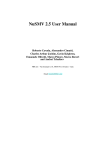
Falcon protection system by Engineering Office Urho Tuominen (UTU) can be used to protect switchgear and electrical instrumentation from electric arcs. The system consists of a master unit, overcurrent sensor units, and light sensor units. Sensors are installed into the protected system and connected
to the master unit via optical cables. The master unit collects the alarm signals from sensors, and when
necessary, launches circuit breakers which close the power feed from the protected device leading to
the termination of the electric arc. This basic setting is illustrated in Figure 1.
The master unit is based on a Programmable Logic Controller (PLC) so that one can freely design
and program the tripping logic according to the protected system and the protection required for it.
This provides the possibility for selective tripping: the protected system can be divided into several
protection zones with different tripping conditions. Falcon system also provides a possibility for
controlling backup breakers which can be launched in the case of a malfunction in a primary breaker.
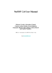
Figure 2 shows an example of a tripping logic of the Falcon system. The figure also shows the input
and output ports of the master unit. For attaching sensor units there are four regular input ports. In
addition, there is also a so-called “extra light board” with an additional 16 inputs which are meant for
light sensors. However, the signals from these ports are combined optically before they are transmitted
to the controller, so from the perspective of tripping logic these input ports correspond to a single input
port.
The number of output ports of the master unit is 10. Four of these are based on fast TRIAC semiconductors and are meant for launching the primary circuit breakers. The other six outputs are based on
ordinary relays and are used for launching backup relays and alarm signals for operators.
The basic programming of a tripping logic is done simply by connecting signals with logical AND and
OR gates. If backup breakers are used, delay gates of a certain type are also needed. This is because
A1
Figure 1: The Falcon Protection System.
A2
Figure 2: A tripping logic of the Falcon system.
A3
backup breakers might typically cover more than one protection zone and therefore they are supposed
to be launched only after it is evident that the primary breakers covered by it have been broken. This
is done by transmitting the launch signal of a backup breaker through such a delay gate which passes
an output signal only once it has received an input signal continuously for a certain time period. Now,
the delay of a delay gate corresponding to a certain backup breaker has to be longer than the physical
activation time of the primary breakers protected by the backup breaker. In this way it is guaranteed
that a backup breaker is not launched before the primary breakers protected by it have had enough
time to have closed the power feed of the protection zone (and terminated the cause of the alarm, i.e.,
the electric arc) if they are not broken.
A.1.3
Study Objectives
The main purpose of this case study was to find out what kinds of verification needs a typical safety
instrumented system introduces, and moreover, on what level one has to model the system to be able to
verify the properties of interest with the chosen tool. The special characteristic of the chosen NuSMV
model checker [1] is that it is not specifically designed for model checking of real-time properties.
However, non-real-time model checkers are capable of handling larger systems than real-time model
checkers, so for this reason one of our main research goals was to find out whether a typical safety
instrumented system can be modelled in such a way that relevant real-time properties can also be
model checked with NuSMV.
Safety instrumented systems introduce two different types of verification tasks. In the first class there
are tasks of verifying that an implementation of the control logic conforms to its specification. This
type of a verification task is presented in Section A.4. The other type of verification tasks consist of
verifying the correctness of a system design. This type of a task is presented in Section A.5.
A.2 An Abstract Model of Safety Instrumented Systems
In this section we present an abstract model for safety instrumented systems (SIS). This model is a
generic model for the kinds of systems to which the model checking method that we used with the
Falcon system can be applied. We refer to this abstract model later in the text while we describe the
modelling process of the Falcon system. Therefore, the abstract model can be used to explain what
kinds of systems our method applies to and as a reference point for new modelling processes. The
abstract model is depicted in Figure 3 and described in the following.
Time model
The time model of the system is discrete. That is, the time increases only in discrete time steps and
the values of the state variables are only read and altered at those time instants. This follows from
the fact that the controller of the SIS is assumed to operate with a constant scan cycle (a scan cycle
of a controller is a single operational period during which the controller reads new inputs, executes
the program and returns new output values). Therefore, a single time step in the abstract model
corresponds in the real world to the length of a single scan cycle of the controller.
Structure of the model
The whole system consists of the controller part which abstracts the controller of the SIS and of the
system environment which abstracts the protected system, as well as the physical environment which
A4
1..n steps
0 steps
D
D
Logic
D
Delays
Controller
0 steps
Inputs
Logic
1 step
M
M
M
Memory
System environment
Figure 3: An abstract model of a SIS.
A5
might affect the state or operation of the SIS.
The controller consists of a logic part and delays. The logic part does not include any state variables,
but it merely calculates the output values as a function of the input values received from the environment. The delays are associated with a delay length (number of time steps) and they operate in such
a way that a delay only passes an output signal if it has received an input signal for the delay length
associated to it. The delay length is at minimum one time step, since the physical controller spends at
minimum one scan cycle between receiving input values and passing output values.
The environment consists of a logic part, memory elements and inputs. The logic part encodes the
behaviour of the environment model, i.e., it calculates the state of the environment model as a function
of the state of the environment on the previous time step and of the inputs to the environment at the
current time step. The memory elements hold the information of the state of the environment on the
previous time step. The inputs correspond to the kinds of information of the physical world which
cannot be deduced from the model. As an example, consider alarm signals or malfunctions of devices,
etc.
A.3 Description of NuSMV Model Checker
In this section we describe the NuSMV model checker [1] which was used to model check the Falcon
case study. Section A.3.1 gives a general overview of NuSMV, Section A.3.2 describes how models
are build with the input language of NuSMV, and Section A.3.3 describes how verified properties are
specified with the input language of NuSMV. The discussion on the syntax and semantics of the input
language of NuSMV covers only the parts of the language which are used in this study. For further
information we advise the reader to see the NuSMV user manual [2].
A.3.1
General Overview
NuSMV is an academic model checker maintained by ITC-IRST. NuSMV can be used to describe
finite state systems that range from completely synchronous to completely asynchronous. The main
reason for choosing NuSMV was that it is a state-of-the-art model checker which has proven to
be capable of handling industrial-sized systems. Moreover, NuSMV supports both BDD (Binary
Decision Diagram) and SAT1 (propositional satisfiability) based model checking which are currently
the main approaches in implementing model checking tools. Being distributed under OpenSource
licence, NuSMV also offers a promising platform for research purposes.
A.3.2
Modelling with NuSMV
General Structure of NuSMV Models
NuSMV models (also referred to as NuSMV programs) consist of one or more module declarations.
A module declaration is an encapsulated collection of declarations, constraints, and specifications.
Intuitively, the idea of the module concept is to encapsulate closely related state variables together
in order clarify the structure of the whole model. Modules are used in such a way that a module
declaration is used as a variable type to create module instances. Therefore, multiple realisations of
a module can be created based on a single module declaration. A module declaration may contain
1
Some of the SAT based model checking algorithms inside NuSMV have been developed at TKK/TCS [3]
A6
instances of other modules so that the modules form a hierarchical structure. Each NuSMV model is
built on a declaration of a special module which has to be named as main.
Next we describe the basic constructs needed for creating module declarations. The description is
based on the NuSMV model shown in Figure 4, which has two module declarations. The model is
complete and it introduces all structures used in our actual case study.
MODULE exampleModule(param1,param2)
VARS
var1 : boolean;
var2 : -1 .. 10;
var3 : -1 .. 10;
ASSIGN
-- An example of direct assignment.
var1 := param1;
-- An example of recursive assignment.
init(var2) := 0;
next(var2) := param2;
init(var3) := -1;
next(var3) :=
case
(var3 < 10) : var3 + 1;
(var3 = 10) : {-1,10};
esac;
MODULE main()
VARS
moduleInstance : exampleModule(definedConstant, 5);
DEFINE
definedConstant := 1;
----------------------------Specification of properties
LTLSPEC G (moduleInstance.var1 -> O (moduleInstance.var2 = 10))
LTLSPEC F (moduleInstance.var2 > moduleInstance.var3)
Figure 4: An example of a NuSMV model.
Structure of a Module Declaration
A description of a NuSMV module consists of several different segments containing different kinds of
declarations, specifications, and constraints. In this case study, only the most central constructs were
needed. These include the parameters of modules, the declaration and assignment of state variables,
and define declarations. These are described in the following.
Parameters of a module. Parameters are defined as a list of identifiers which can be used for
passing data to a module from other modules. The parameters of a module are specified with a parenthesised list of identifiers following the name of a module (see param1 and param2 in the example
above. The main module is not allowed to have parameters.
A7
State variables of a module. The state variables of a module are listed in a segment identified with
the keyword VAR. A state variable declaration consists of an identifier which can be used to refer to
the variable and a type specification which describes the data type and the range of possible values of
the variable. As data types one can use either built-in data types or module declarations.
In our case study, only two built-in data types, boolean and integer, are used. The boolean data type
comprises two integer values, 0 and 1 (or their symbolic counterparts false and true respectively.)
The value range of the integer type consists of integer values from −232 + 1 to 232 − 1. The integer
type is specified by declaring a value range after the variable identifier (see declaration of var2 in the
exampleModule.)
If a module declaration is used as a data type in a variable declaration, the variable is said to be
an instance of the module, and the variable declaration is said to be a module instantiation. The
declaration is formed simply by referring to the module name (followed by a list of parameters) in the
place of the variable type (see variable moduleInstance of the main module in Figure 4.)
Assignment of state variables. State variables are assigned in a segment identified with the keyword ASSIGN. A state variable can be assigned in two distinct ways, either directly or with an
init/next construct. The variable var1 in the exampleModule in Figure 4 shows an example of
direct assignment. In this case, the value of the current value of the var1 is set to the value of parameter param1.
In the case of the variable var2 in the exampleModule, the assignment is done using the init/next
construct. In this case, the assignment is done in two steps: first the initial value (i.e., the value of the
state variable at the first time step, or in the initial state) of var2 is set to zero. On the following line,
it is stated that the value of var2 in the next state will be the value of param2.
The variable var3 in the exampleModule is defined as var2 but in its next-expression another two
important constructs related to assignments are shown: the case expression and the set expression.
The segment surrounded by keywords case and esac define a case expression. It can be used to
express that the value assigned to a state variable depends on the condition of other state variables.
Each line of the case segment has on its left-hand side a boolean valued condition statement and on
its right-hand side a value which is assigned to the state variable if the condition holds. The lines are
evaluated sequentially one-by-one starting from the first line until the first line whose condition part
is equals to 1 is reached. If the conditions of each line in the case statement are equal to 0, then an
arbitrary value belonging to the value range of the state variable is assigned to it.
In the case of var3, the case statement increases its value in the next state by one if the current value
is below the value 10 (which is the maximum value it can have). If the current value of var3 is 10, its
value in the next state is chosen non-deterministically from the set expression {0, 10}. Consequently,
a set expression is a way of stating that the value used in the assignment can be chosen among a set
of values. The choice can be done freely and, in fact, as NuSMV carries out an exhaustive search, all
of the specified values in a set expression will be examined in turn.
DEFINE declarations Define declarations are yet another basic construct used to build modules.
Define declarations are added in a module declaration after the keyword DEFINE and they are used
to associate a common expression with a symbol. That is, the define declarations are used to define
shorthands for complex expressions or numeric values in order to make module descriptions more
A8
concise. The defineConstant of the main module in Figure 4 shows an example of define declaration in which the numeric value 1 is associated with an identifier.
A.3.3
Specification of Properties
The properties of this study are specified by using Linear Temporal Logic extended with past operators
(hereafter LTL). Also invariant specifications are used, but they can be formulated in LTL as well. In
this section we describe the syntax of LTL in NuSMV.
In NuSMV, LTL formulas are used to specify conditions or relations between the state variables of
a NuSMV model. The specifications are formed by connecting state variables with LTL operators
which include the basic logical boolean operators and special temporal operators which can be used
to specify time related statements.
The following list containts the LTL operators of NuSMV used in this study and describes their semantics informally. More extensive coverage of LTL with past operators can be found in addition to
the NuSMV user manual [2] from [3] by Heljanko, Junttila, and Latvala.
NuSMV syntax of boolean operators:
!x (logical not): !x is true if x is not true.
x & y (logical AND): x & y is true if x is true and y is true.
x | y (logical OR): x | y is true if x is true or y is true.
→ (implication): x → y is true if y is true whenever x is true.
↔ (equivalence): x ↔ y is true if the values of x and y are equal.
NuSMV syntax of temporal operators of LTL with past operators:
G (globally): G f is true if f is true at all time steps.
F (finally): F f is true at this time step if f will be true at some time step in the future.
O (once): O f is true if f is true at this time step or has been true at some previous time step.
Y (previous state): Y f is true if f was true at previous time step.
In the example model of Figure 4, two examples of LTL property specifications are shown. The first
property states that “in all time steps it holds that if the value of var1 of moduleInstance is true,
then there has to be a time step in the past in which the value of var2 of moduleInstance was 10”.
The second property states that “there has to be some time step in which it holds that the value of
var2 of moduleInstance is bigger than the value of var3 of moduleInstance.”
A9
A.4 Verifying the Implementation of Control Logic
A.4.1
Overview on the Verification Task
Here we present an example of the task of verifying whether an implementation of control logic conforms to its specification. In this context, by a specification we mean a description of the input/output
behaviour of the control logic. That is, a specification describes what output signals the controller
should return for each possible input combination. The verification task introduced is to verify that
an implementation built on a specification actually behaves precisely according to the specification.
With respect to the abstract model presented in Section A.2, only the Logic part of the Controller in
Figure 3 is considered.
The verification was carried out on a real system description provided by UTU. Figure 5 shows the
implementation of the control logic which is based on the specification document shown in Figure 6.
A.4.2
Description of the NuSMV Model
The NuSMV model consist simply of two modules named TruthTable and Falcon which encode
the specification and the implementation (respectively) of the control logic. The structure of both of
the modules is very similar. Both have the inputs of the Falcon master unit as parameters and both
include boolean state variables for the four output signals used in the control logic. In the case of the
Falcon module, the logic is encoded conveniently by introducing a define declaration for each of the
logical gates of the tripping logic and by using these declarations with the assignments of the state
variables.
In the case of the TruthTable module, the state variable assignments were done by encoding the
rows of the specification document directly into case expressions.
A.4.3
Specification of Properties with NuSMV
With this verification task only one property needed to be specified. It is an invariant specification
which states that with all possible combinations of inputs, the outputs have to be the same. This
property is specified in the input language of NuSMV in the following way:
LTLSPEC G ((falcon.triac1
(falcon.triac2
(falcon.triac3
(falcon.relay6
A.4.4
<->
<->
<->
<->
truth_table.triac1) &
truth_table.triac2) &
truth_table.triac3) &
truth_table.relay6))
Full Source Code of the NuSMV Model
-------------------------------------------------------------------------MODULE Falcon(ch1,ch2,ch3,ch4,lights)
VAR
triac1 : boolean;
triac2 : boolean;
triac3 : boolean;
relay6 : boolean;
DEFINE
A10
Figure 5: Tripping logic diagram of the example system.
A11
Figure 6: Truth table representation of the specification of the tripping logic of the example system.
or_gate0 := ch1 | ch3;
and_gate0 := or_gate0 & ch2;
and_gate1 := or_gate0 & ch4;
and_gate2 := or_gate0 & lights;
or_gate1
or_gate2
or_gate3
or_gate4
:=
:=
:=
:=
and_gate0
and_gate1
and_gate0
and_gate0
|
|
|
|
and_gate1 | and_gate2;
and_gate2;
and_gate1;
and_gate1 | and_gate2;
ASSIGN
init(triac1)
init(triac2)
init(triac3)
init(relay6)
:=
:=
:=
:=
0;
0;
0;
0;
next(triac1)
next(triac2)
next(triac3)
next(relay6)
:=
:=
:=
:=
or_gate1;
or_gate2;
or_gate3;
or_gate4;
-------------------------------------------------------------------------MODULE TruthTable(ch1,ch2,ch3,ch4,lights)
VAR
triac1 : boolean;
A12
triac2 : boolean;
triac3 : boolean;
relay6 : boolean;
ASSIGN
init(triac1)
init(triac2)
init(triac3)
init(relay6)
:=
:=
:=
:=
0;
0;
0;
0;
next(triac1) :=
case
-- Truth table rows with output value
!ch1 & !ch2 & !ch3 & !ch4 & !lights :
!ch1 & !ch2 & !ch3 & !ch4 & lights :
!ch1 & !ch2 & !ch3 & ch4 & !lights :
!ch1 & !ch2 & !ch3 & ch4 & lights :
!ch1 & !ch2 & ch3 & !ch4 & !lights :
0.
0;
0;
0;
0;
0;
------
row
row
row
row
row
1
2
3
4
5
:
:
:
:
0;
0;
0;
0;
-----
row
row
row
row
9
10
11
12
ch1 & !ch2 & !ch3 & !ch4 & !lights :
ch1 & !ch2 & ch3 & !ch4 & !lights :
-- Truth table rows with output value
1
:
esac;
0;
0;
1.
1;
-- row 17
-- row 21
!ch1
!ch1
!ch1
!ch1
&
&
&
&
ch2
ch2
ch2
ch2
&
&
&
&
!ch3
!ch3
!ch3
!ch3
&
&
&
&
!ch4
!ch4
ch4
ch4
&
&
&
&
!lights
lights
!lights
lights
next(triac2) :=
case
-- Truth table rows with output value
!ch1 & !ch2 & !ch3 & !ch4 & !lights :
!ch1 & !ch2 & !ch3 & !ch4 & lights :
!ch1 & !ch2 & !ch3 & ch4 & !lights :
!ch1 & !ch2 & !ch3 & ch4 & lights :
!ch1 & !ch2 & ch3 & !ch4 & !lights :
!ch1
!ch1
!ch1
!ch1
!ch1
&
&
&
&
&
ch2
ch2
ch2
ch2
ch2
&
&
&
&
&
!ch3
!ch3
!ch3
!ch3
ch3
&
&
&
&
&
ch1 & !ch2 & !ch3 &
ch1 & !ch2 & ch3 &
ch1 & ch2 & !ch3 &
ch1 & ch2 & ch3 &
-- Truth table rows
1
: 1;
esac;
!ch4
!ch4
ch4
ch4
!ch4
!ch4
!ch4
!ch4
!ch4
with
0.
0;
0;
0;
0;
0;
------
row
row
row
row
row
1
2
3
4
5
:
:
:
:
:
0;
0;
0;
0;
0;
------
row
row
row
row
row
9
10
11
12
13
& !lights :
& !lights :
& !lights :
& !lights :
output value
0;
0;
0;
0;
1.
-----
row
row
row
row
17
21
25
29
&
&
&
&
&
!lights
lights
!lights
lights
!lights
next(triac3) :=
case
-- Truth table rows with output value 0.
A13
!ch1
!ch1
!ch1
!ch1
!ch1
!ch1
&
&
&
&
&
&
!ch2
!ch2
!ch2
!ch2
!ch2
!ch2
&
&
&
&
&
&
!ch3
!ch3
!ch3
!ch3
ch3
ch3
&
&
&
&
&
&
!ch4
!ch4
ch4
ch4
!ch4
!ch4
&
&
&
&
&
&
!lights
lights
!lights
lights
!lights
lights
:
:
:
:
:
:
0;
0;
0;
0;
0;
0;
-------
row
row
row
row
row
row
1
2
3
4
5
6
!ch1
!ch1
!ch1
!ch1
&
&
&
&
ch2
ch2
ch2
ch2
&
&
&
&
!ch3
!ch3
!ch3
!ch3
&
&
&
&
!ch4
!ch4
ch4
ch4
&
&
&
&
!lights
lights
!lights
lights
:
:
:
:
0;
0;
0;
0;
-----
row
row
row
row
9
10
11
12
ch1 & !ch2 & !ch3 & !ch4 & !lights :
ch1 & !ch2 & !ch3 & !ch4 & lights :
ch1 & !ch2 & ch3 & !ch4 & !lights :
ch1 & !ch2 & ch3 & !ch4 & lights :
-- Truth table rows with output value
1
:
esac;
0;
0;
0;
0;
1.
1;
-----
row
row
row
row
17
18
21
22
0.
0;
0;
0;
0;
0;
------
row
row
row
row
row
1
2
3
4
5
:
:
:
:
0;
0;
0;
0;
-----
row
row
row
row
9
10
11
12
ch1 & !ch2 & !ch3 & !ch4 & !lights :
ch1 & !ch2 & ch3 & !ch4 & !lights :
-- Truth table rows with output value
1
:
esac;
0;
0;
1.
1;
-- row 17
-- row 21
next(relay6) :=
case
-- Truth table rows with output value
!ch1 & !ch2 & !ch3 & !ch4 & !lights :
!ch1 & !ch2 & !ch3 & !ch4 & lights :
!ch1 & !ch2 & !ch3 & ch4 & !lights :
!ch1 & !ch2 & !ch3 & ch4 & lights :
!ch1 & !ch2 & ch3 & !ch4 & !lights :
!ch1
!ch1
!ch1
!ch1
&
&
&
&
ch2
ch2
ch2
ch2
&
&
&
&
!ch3
!ch3
!ch3
!ch3
&
&
&
&
!ch4
!ch4
ch4
ch4
&
&
&
&
!lights
lights
!lights
lights
-------------------------------------------------------------------------MODULE main
VAR
ch1 : boolean;
ch2 : boolean;
ch3 : boolean;
ch4 : boolean;
lights : boolean;
falcon : Falcon(ch1,ch2,ch3,ch4,lights);
truth_table : TruthTable(ch1,ch2,ch3,ch4,lights);
ASSIGN
init(ch1) := {0,1};
init(ch2) := {0,1};
init(ch3) := {0,1};
A14
init(ch4) := {0,1};
init(lights) := {0,1};
next(ch1) :=
next(ch2) :=
next(ch3) :=
next(ch4) :=
next(lights)
{0,1};
{0,1};
{0,1};
{0,1};
:= {0,1};
--------------------------------------------------------------------------- Specification of properties
-- The outputs of the modules
LTLSPEC G ((falcon.triac1 <->
(falcon.triac2 <->
(falcon.triac3 <->
(falcon.relay6 <->
have to be equal with all inputs.
truth_table.triac1) &
truth_table.triac2) &
truth_table.triac3) &
truth_table.relay6))
A.5 Verifying the Correctness of System Design
In Section A.4 we showed how it can be verified that the control logic of the Falcon system conforms
to its specification. In contrast, here we show how the correctness in the design of a whole system
can be verified. That is, we want to verify that a protection system based on a certain control logic
operates as intended with respect to the system it protects.
The section is organised as follows: Section A.5.1 describes the properties which the system is required to fulfil in order that the design is considered to be correct. Section A.5.2 describes the types of
information required from the system that the model checking can carry out. Section A.5.3 describes
the specific application of the Falcon system which was used in the case study. Section A.5.4 describes
what kinds of assumptions one needs to make on the system so that it can be modelled. Section A.5.5
gives an overview of the NuSMV model of the case study and Section A.5.6 explains how the verified
properties are specified in the input language of NuSMV. Section A.5.7 presents some experimental
results of the running times of the model checking of the case study with different parameter values.
Finally, in Section A.5.8, the full source code of the NuSMV model with the property specifications
is presented.
A.5.1
Verified Properties
In the case of the Falcon system, the most important property to be verified is that the system does
not make unnecessary tripping decisions. This is because the system is often used to protect, for
example, large manufacturing plants for which an unnecessary shutdown caused by an unnecessary
tripping decision might cause very high expenses.
In order to avoid any false trips, the following properties have to hold:
p1: The couplings and the tripping logic have to conform to the specified tripping conditions.
p2: The backup breakers should not be tripped unless necessary.
The requirement of the absence of unnecessary tripping decisions falls into the category of safety
properties as it states that the system should not do anything unwanted. Another type of properties
A15
called liveness properties informally state that the system should always perform the task that it is
designed for. In the case of the Falcon system, this would be stated as the following requirement:
p3: Existence of an electric arc on the protected system leads eventually to shutting down the power
feed for the protected system.
These properties are the most relevant requirements for the Falcon system. In the following section
we list the the types of information and documents needed in order to be able to verify these properties
with the aid of model checking.
A.5.2
Information Required for Verification
Here we describe what sorts of information one needs in order to model check the properties of the
Falcon system:
1. Description of the specific application
In case of verifying the correctness of the system design of a safety instrumented system, the
question is of verifying whether the control logic of a controller is designed correctly with
respect to the environment in which the controller is installed. Therefore, in this case it is not
sufficient to model only the control logic of the controller, but one also has to build a model of
the environment of the controller. For this reason, besides the control logic, we need now also
a switch diagram and a system description with the following information:
• What is the structure of the protected system (structure of the power-distribution network,
location of the power feeds, transformers, circuit breakers)?
• How the sensor units are installed into the protected system?
• Into what kinds of protection zones the protected system is divided?
• What are the tripping conditions of the protection zones?
• Which circuit breakers need to be launched in order to disable the power feed from the
protection zones?
• Are there any backup circuit breakers, and if so, what are their tripping conditions?
2. Assumptions about the whole system
The information listed in the previous item describes the architectural structure of the protected
system and the installation and intended operation model of the protection system. However, for
the modelling of the whole system, one also needs to clarify all relevant physical and functional
properties on both the protection system and the protected system. A few examples of the things
to be clarified in the case of the Falcon system are:
• What kinds of delays there are with the devices of the system?
• In which parts of the protected system can short circuits occur?
• What are the failure modes of the associated devices?
Because all aspects of the physical world cannot be modelled, one has to make assumptions on
the physical system so that the physical model can be stated to conform to the model in case
the assumptions hold.
A16
These kinds of detailed descriptions of the system might not be available in the existing documentation neither in the case of the protected or the protection system. Therefore, with critical
applications, the modelling of the system should always be carried out in cooperation with
domain specialists.
3. List of unambiguously defined requirements to be verified
In the previous section the verified properties of the Falcon system were listed on a general
level. However, in order to perform model checking, the properties have to be described more
precisely so that there are no questions about how the properties should be interpreted. In this
case, for example, one needs to state precisely when a tripping decision is unnecessary. In the
Section A.5.6, it is shown how the verified properties are refined so that they can be stated in
the terms of the formal model of the system.
Unfortunately a complete set of all this information concerning a single specific application of
the Falcon system was not available. Therefore we designed our own application on the basis of the
documents we received from UTU and which related to several different applications. Our model was
reviewed by UTU representatives and it was considered to be fully realistic in all aspects.
A.5.3
Description of the Application
A.5.3.1 Architecture of the System
Our fictional application of the Falcon system is shown in Figure 7. The system consists of the
protected system and the Falcon system. The protected system consists of the following things:
• main power feeds pf1 and pf2,
• transformers tr1, tr2, tr3, and tr4,
• primary circuit breakers A, B, C, and D,
• backup circuit breakers E, F, H, and G, and
• protection zones 1, 2, and 3.
The Falcon system introduces the following elements into the whole system:
• the Falcon master unit,
• overcurrent sensors Cr1, Cr2, Cr3a, and Cr3b, and
• light sensors L1, L2, and L3.
A.5.3.2 Operation of the System
The main power feeds pf1 and pf2 distribute electricity to the protected system. They are connected
to each other by a switch operated by the circuit breaker C, and therefore, they act as each others
backup systems. That is, both pf1 and pf2 can deliver power to the whole protected system alone if a
malfunction occurs in one of them.
The protected system is divided into three distinct protection zones. For all of these there is a zonespecific tripping condition which causes tripping of circuit breakers that leads to the isolation of
A17
Falcon
pf1 (110 kV)
pf2 (110 kV )
Breaker E
Breaker F
Breaker H
Breaker G
tr1
tr2
Cr3b
Cr3a
Current
Current
Breaker D
20 kV
20 kV
Breaker C
tr3
L3
tr4
Light
Cr2
Current
Cr1
Zone 3
Current
Breaker B
Breaker A
L2
L1
Light
Light
Zone 2
Zone 1
Figure 7: Switch diagram of the example system.
A18
the protection zone from the power feed. The protection system is designed to operate with each
protection zone so that there are two “levels” of backup breakers. That is, if the primary breakers are
broken, the protection system first tries to cut down the power feed only from the main power feed
which is closest to the alarming zone (the “first level”). If the alarm is still on (which might result
e.g., if the connecting breaker C was broken), then the power feed will be cut also from the other
main power feed which will lead to the power feed from the whole system (presumed that the backup
breakers are working correctly) being cut off.
The tripping conditions and related actions are listed in the Table 1 and in Figure 8 a tripping logic
which is created based on this table is presented. The delays D1 and D3 are related to the backup
breakers of the “first level” and delays D2 and D4 are related to the “second level”. Therefore, it
should be that D1 < D2 and D3 < D4.
Alarm
Cr1 AND L1
(alarm on zone 1)
Cr2 AND L2
(alarm on zone 2)
(Cr3a OR Cr3b) AND L3
(alarm on zone 3)
First action
Breakers A and C launched
Breakers B and C launched
Breakers C and D launched
Second action
Breaker E launched
(after delay D1)
Breaker E launched
(after delay D1)
Breaker G launched
(after delay D3)
Third action
Breaker F launched
(after delay D2)
Breaker F launched
(after delay D2)
Breaker H launched
(after delay D4)
Table 1: Actions caused by alarms on different protection zones.
Cr1 AND L1
Triac 1
-> Breaker A
Cr2 AND L2
Triac 2
-> Breaker B
Triac 3
-> Breaker C
OR
Cr3a
OR
Cr3b
Triac 4
-> Breaker D
AND
L3
OR
D1
Relay 1
-> Breaker E
200
D2
Relay 2
-> Breaker F
100
D3
Relay 3
-> Breaker G
200
D4
Relay 4
-> Breaker H
Figure 8: Tripping logic of the example system.
A19
A.5.4
Assumptions of the System
In the previous section the structure and operation of the example system was described. However,
in order to be able to carry out the modelling process, we also need to make some assumptions about
the functional and behavioural properties of the system. Here is the list of assumptions made on the
example system.
General assumptions:
• The duration of one operation cycle of the controller of the Falcon master unit, i.e., time during
which the Falcon system detects an alarm signal through a sensor and passes a launch signal to
a circuit breaker is 1 millisecond. (This time period will correspond to a single time step in the
model of the system, so it is of great importance.)
• The physical devices excluding the primary circuit breakers cannot break down.
Overcurrent alarms:
• Overcurrent peaks detected by the overcurrent sensors are caused by short circuits.
• Short circuits can arise only in the parts of the protected system which are defined as protection
zones.
• Overcurrent peaks cannot move through the transformers.
• An overcurrent sensor can raise an alarm signal anytime as long as it is connected to the protection zone it is overseeing and the protection zone is still connected to a power feed. If these
conditions are not met, the overcurrent sensor cannot raise an alarm.
Light alarms:
• A light sensor can raise an alarm signal nondeterministically at any given time instant, i.e., light
alarms are independent of the rest of the system.
Circuit breakers:
• Once a circuit breaker has been activated, it opens the electric circuit and prevents the flowing
of the current.
• An activated circuit breaker will remain activated forever.
• There is an activation delay associated with each circuit breaker, which is the time period
between the moment when a breaker is launched and the moment when it has opened the circuit
preventing the electric current flowing. (The model checking was carried out with different
parameter values for the size of the activation delay, see Section A.5.7.)
• A non-activated primary circuit breaker can break down at any given time.
• A broken circuit breaker cannot open a circuit.
• A broken circuit breaker will stay broken forever.
A20
A.5.5
Description of the NuSMV Model
In this section we give an overall description on how the Falcon system and it’s environment was modelled with NuSMV. The text is organised according to the abstract SIS model covered in Section A.2.
We describe for each part of the abstract model which parts of the Falcon system correspond to it.
Moreover, we give an overall description on how these parts of the Falcon system were modelled with
NuSMV. In the following text we will refer to the parts of the abstract model with the “abstract”-prefix
to emphasise the distinction between corresponding parts of the Falcon system or the NuSMV model.
We begin the discussion from the Controller part of the abstract model and then proceed to the System
environment. The NuSMV modules described in the following are also illustrated in Figure 9 which
depicts the data flow between the modules.
Controller
Controller module
Delay
modules
Overcurrent sensor
modules
Current flow model
Breaker modules
Timer
modules
Inputs (overcurrent alarm)
Inputs
(malfunctions)
Light sensor modules
Inputs (light alarm)
System environment
Figure 9: Data flow between NuSMV modules.
Controller
In the case of the Falcon system, the master unit corresponds to the Controller part of the abstract
SIS model. The Falcon counterpart for the logic part of the abstract model is the logical circuit of the
tripping logic excluding the delay gates. The delay gates correspond to the delays of the controller in
the abstract model.
In our NuSMV model there is a module declaration for encoding the delays and a module for encoding
the controller part. They are described in the following.
Delay module:
The Delay module has two parameters: boolean valued input signal and a delay value whose
A21
type is non-negative integer (it should be noted here, that NuSMV does not allow explicit type
declarations for module parameters, but type checking is carried out implicitly.) The module
has a boolean valued variable representing the output signal of the abstract delay.
The operation logic of the Delay module is based on an integer valued counter whose values
may vary between zero and the value of the parameter delay. The counter is set to zero whenever
the input signal is 0. If the input signal is 1, the counter is increased until it reaches the value
of the delay parameter. The value of the output signal is assigned to 1 only if the counter has
reached the value of the delay parameter.
Controller module:
A module implementation corresponding to the Controller part of the abstract model would
have boolean valued parameters for each input signals of the abstract Controller, one instance
of a Delay module described above for each delay of the abstract Controller, and two constant
definitions for the input and output values for each delay of the abstract Controller. The input values of the delays are, at the same time, the output values of the Logic of the abstract
Controller and they are defined as functions of the parameters of the Controller module. These
functions encode the logic of the abstract Controller. After the values of the input constants have
been assigned, they are set as the parameters for the delay instances. The values of the output
constants are set to hold the values of the outputs of the delay instances, i.e., they represent the
values of the output signals of the Controller part of the abstract model.
In the case of the Falcon system, the Controller module has five parameters (in the actual system
the 16 inputs of the light board are combined into a single signal with an optical OR). For
each output of the Falcon Master unit there is an instance of the Delay module and constant
definitions for input and output values as described above.
The delay parameter values of the Delay module instances are set to values ⌈D/t⌉ where D is
the delay in milliseconds of the corresponding delay gate in the Falcon tripping logic and t is
the length (also in milliseconds) of the operation cycle of the controller of the Falcon master
unit. In practice, the parameter value is the physical delay in milliseconds since the operation
cycle of the Falcon master unit is 1ms as stated in Section A.5.4.
System environment
In the case of the Falcon system, the system environment of the abstract model breaks down to the
protected system (divided into one or more protection zones), primary and backup circuit breakers,
and the sensor units of the Falcon system.
The logic of the system environment consists of the following things:
• operational and failure models of the breakers,
• operational model of the sensors, and
• reasoning of whether each protection zone is connected to a power feed.
The memory elements of the abstract system environment are used for holding the state of the system
environment in the previous time step. In the case of the Falcon system, these states are related to the
A22
circuit breakers. That is, for each circuit breaker we need to know whether the following things held
in the previous time step:
• is the breaker broken,
• has the breaker launched, and
• is the breaker activated.
In the case of the Falcon system, the inputs of the system environment are:
• overcurrent and light signals, and
• the information of break-ups of the primary breakers.
The NuSMV model of the system environment consists of two distinct modules for light and overcurrent sensors, a module for circuit breakers (the same module is used for both primary and backup
breakers), a module for encoding a counter representing the activation delay of the breakers, and
constant definitions for the current flow model. In the following we give an overview on how these
entities were implemented.
Timer module:
The Timer module has the same parameters as the Delay module described above: a boolean
valued input signal and a delay value whose type is non-negative integer. It also defines the
output signal as a boolean valued variable. As the Delay module, the Timer module is also
based on a integer valued counter which measures the number of steps passed. However, the
logic of the counter is different: Initially the counter is set to the value of the delay parameter
and it stays at that value until the input signal is 1. After this, regardless of the value of the
input signal, the counter is decreased by one until it reaches the value zero, after which it is set
back to the value of the delay parameter. The output value of the module is set to 1 only at the
time when the value of the counter is set to 0.
Breaker module:
The Breaker module has three parameters: Boolean valued launch signal, a delay which is nonnegative integer, and a boolean valued flag which specifies whether the breaker can get broken
or not (in order to simplify the model, the backup breakers are not allowed to break down.)
The Breaker module has two boolean variables which tell whether the breaker is active or not,
and whether the breaker is broken or not. It also has an instance of the Timer module which
represents the activation delay of the breaker.
The activation delay of the breaker is determined with the delay parameter passed to the instance
of the Delay module. This parameter should be ⌈D/t⌉ where D is the physical activation delay
(in milliseconds) of the corresponding real circuit breaker and t is the length (in milliseconds)
of the operation cycle of the controller of the Falcon master unit. In practice, the parameter
value is the physical delay in milliseconds since the operation cycle of the Falcon master unit
is 1ms as stated in Section A.5.4.
Light sensor module:
The light sensor module does not have any parameters and it only has one boolean variable
which represents a light alarm. The light sensor could be defined simply as a boolean variable
but it is defined as a module so that it is uniform with the implementation of the overcurrent
sensor.
A23
Overcurrent sensor module:
The Overcurrent sensor module has two boolean valued parameters which describe whether the
sensor is still connected to the protection zone that it is observing and whether the protection
zone is still connected to the power feed. The module has a boolean variable representing an
overcurrent signal.
Current flow model implementation:
The current flow model is implemented in such a way that there is a constant definition corresponding to each of the three protection zones which tell whether the zone is connected to a
power feed or not. The value of the constant corresponding to a certain protection zone is set
to 1 if there is at least one closed circuit line connecting the protection zone to a power feed.
Therefore, the zone constants are functions of the output values of the circuit breakers which
tell whether the circuit breaker is active or not.
We also included one additional constant definition for each protection zone which tells whether
the tripping condition of a zone is trueat each time step. These constants are not indispensable
but with them the specification of properties becomes more convenient.
A.5.6
Specification of Properties with NuSMV
In this section it is shown how the properties described in Section A.5.1 are specified with the input
language of the NuSMV model checker. However, first we refine and specify each property in as
specific form as is needed for the formal specification to be possible.
Safety properties
The first safety property p1 of Section A.5.1 states that the couplings of the system and tripping logic
are done correctly. In the case of the primary breakers, this property is formulated specifically in the
following way:
If a primary circuit breaker is launched at a certain time step, then the tripping condition of this
breaker was realised in the previous time step.
With NuSMV this is specified as:
LTLSPEC G (LTLSPEC G (breaker_A.launched -> Y zone1_alarm))
In the case of the backup breakers, the property can be formulated more conveniently as follows:
If a backup breaker is launched at a given time step, then one of the primary breakers covered by
it is launched also at the same time step.
With NuSMV this is specified like this:
LTLSPEC G (breaker_E.launched -> (breaker_A.launched | breaker_B.launched))
The second safety property p2 of Section A.5.1 states that the backup breakers should not be launched
unless necessary. This requirement is formulated more precisely in this way:
A24
If a backup breaker receives a launch signal, then at least one of the primary breakers covered by
it has broken down.
With NuSMV this is specified as follows:
LTLSPEC G (breaker_E.launched -> (breaker_A.is_broken | breaker_B.is_broken))
Liveness properties
The liveness property p3 of Section A.5.1 is formulated more specifically like this:
If the protection system receives an alarm from a protection zone in a given instant of time, there
will be a instant of time in the future, when the alarm has either disappeared from the protection zone
or the protection zone is disconnected from the power feed.
With NuSMV this is specified like this:
LTLSPEC G (zone1_alarm -> F (!zone1_alarm | !zone1_hasvoltage))
A.5.7
Experimental Results
In the following we present some measurements on the running times of the model checking of our
example system.
Test Equipment
The model checking was carried out with a PC with 1.8GHz Intel Core 2 Duo E63xx DualCore
processor. Available virtual memory was limited to 1.5 GiB. The operating system used was Debian
GNU/Linux and the model checking was carried out with NuSMV version 2.4.2.
Measurements
The model checking was carried out on the model shown in Section A.5.8. The parameters altered
were the delay parameters D1, D2, D3, and D4 of the tripping logic of the example system (see
Figure 8 and Table 1) and the activation time of the circuit breakers (with each distinct model checking
process the same activation time was used with all the breakers.) As explained in Section A.5.5
(see the descriptions of the Controller and Breaker modules), these parameter values correspond to
milliseconds in real-time. The measurements are shown in Table 2.
The measurements show that the size of the running time grows rather quickly as the function of the
delay parameters. For the activation delay parameter of value 6, roughly half of the properties could
be verified within 24 hours which was set as the maximum processing time for each measurement.
Activation delay
of breakers
2
3
6
D1
D2
D3
D4
Running Time
6
9
18
9
14
27
3
5
9
6
9
18
27 min
4h 20min
>24h
Table 2: Running times of the model checking process with different parameter values.
A25
A.5.8
Full Source Code of the NuSMV Model
--------------------------------------------------------------------------- Delay module is used to model the delay gates of the tripping logic
-- of the Falcon master unit.
-- With delay=0 the relay acts in one cycle. The delay
-- parameter specifies how many additional scan cycles the input has
-- to be TRUE before an output signal TRUE is given.
MODULE Delay(input_signal, delay)
VAR
count : 0..51;
output : boolean;
DEFINE
-- Total delay consist of the delay + scan cycle
total_delay := delay + 1;
ASSIGN
init(count) := 0;
next(count) :=
case
input_signal = 0
count >= total_delay
1
esac;
: 0;
: count;
: count + 1;
init(output) := 0;
next(output) :=
case
-- At the step when count = delay, output has to be 1.
next(count) >= total_delay
: 1;
1
: 0;
esac;
--------------------------------------------------------------------------- Timer module is used by the Breaker module to model the physical
-- activation delay of a breaker.
MODULE Timer(signal,delay)
VAR
counter : 0..15;
DEFINE
output :=
case
(delay = 0) : signal;
(counter = 0) : 1;
1 : 0;
esac;
ASSIGN
init(counter) := delay;
next(counter) :=
case
(delay = 0) : 0;
(counter = 0) : delay;
A26
(counter < delay) : counter - 1;
(counter = delay) & (signal = 1) : counter - 1;
1 : counter;
esac;
--------------------------------------------------------------------------- Breaker module is used to model the physical circuit breakers
-- controlled by the Falcon master unit.
MODULE Breaker(launch_signal, setting_up_time, can_break)
VAR
is_broken : boolean;
cuts : boolean;
timer : Timer(launch_signal,setting_up_time);
DEFINE
launched := launch_signal;
ASSIGN
init(is_broken)
next(is_broken)
case
can_break =
is_broken =
is_broken =
1
esac;
:= 0;
:=
0 : 0;
0 : {0,1};
1 : 1;
: 1;
init(cuts) := timer.output;
next(cuts) :=
case
(cuts = 1) : 1;
(is_broken = 1) : cuts;
(next(timer.output) = 1) : 1;
(next(timer.output) = 0) : 0;
esac;
--------------------------------------------------------------------------- UTU_CR module is used to model the overcurrent sensors of the Falcon
-- system.
MODULE UTU_CR(has_voltage,breaker)
VAR
overcurrent : boolean;
ASSIGN
overcurrent :=
case
!has_voltage | breaker.cuts
1
esac;
: 0;
: {0,1};
A27
--------------------------------------------------------------------------- UTU_ARC module is used to model the light sensors of the Falcon
-- system.
MODULE UTU_ARC()
VAR
light : boolean;
ASSIGN
light := {0,1};
--------------------------------------------------------------------------- Controller module models the Falcon master unit.
MODULE Controller(ch1,ch2,ch3,ch4,ch_light)
VAR
triac1_delay : Delay(tr1_input,TRIAC_DELAY);
triac2_delay : Delay(tr2_input,TRIAC_DELAY);
triac3_delay : Delay(tr3_input,TRIAC_DELAY);
triac4_delay : Delay(tr4_input,TRIAC_DELAY);
time_relay1
time_relay2
time_relay3
time_relay4
:
:
:
:
Delay(r1_input,RELAY1_DELAY);
Delay(r2_input,RELAY2_DELAY);
Delay(r3_input,RELAY3_DELAY);
Delay(r4_input,RELAY4_DELAY);
DEFINE
-- Delay values of the delay gates. These values should be set to
-- the delay values (in milliseconds) of the corresponding delay
-- gates in the modelled tripping logic.
TRIAC_DELAY := 0;
RELAY1_DELAY := 35;
RELAY2_DELAY := 50;
RELAY3_DELAY := 35;
RELAY4_DELAY := 50;
-- Logic of the circuits.
OR1 := (ch3 | ch4);
AND1 := (OR1 & ch_light);
OR2 := (ch1 | ch2 | AND1);
OR3 := (ch1 | ch2);
-- Inputs
tr1_input
tr2_input
tr3_input
tr4_input
r1_input
r2_input
r3_input
r4_input
to
:=
:=
:=
:=
:=
:=
:=
:=
delays.
ch1;
ch2;
OR2;
AND1;
OR3;
OR3;
AND1;
AND1;
-- Outputs of the controller module.
triac1 := triac1_delay.output;
A28
triac2 := triac2_delay.output;
triac3 := triac3_delay.output;
triac4 := triac4_delay.output;
r1
r2
r3
r4
:=
:=
:=
:=
time_relay1.output;
time_relay2.output;
time_relay3.output;
time_relay4.output;
--------------------------------------------------------------------------- main module is the main program of the whole model and it encompasses
-- both, the model of the controller and its environment.
MODULE main
VAR
-- The controller of Falcon master unit
ctrl : Controller(zone1_alarm, zone2_alarm, Cr_3a.overcurrent,
Cr_3b.overcurrent, L_3.light);
-- Overcurrent sensors
Cr_1 : UTU_CR(zone1_hasvoltage,breaker_A);
Cr_2 : UTU_CR(zone2_hasvoltage,breaker_B);
Cr_3a : UTU_CR(zone3_hasvoltage,breaker_C);
Cr_3b : UTU_CR(zone3_hasvoltage,breaker_D);
-- Light sensors
L_1 : UTU_ARC();
L_2 : UTU_ARC();
L_3 : UTU_ARC();
-- Primary breakers
breaker_A : Breaker(ctrl.triac1,
breaker_B : Breaker(ctrl.triac2,
breaker_C : Breaker(ctrl.triac3,
breaker_D : Breaker(ctrl.triac4,
-- Backup
breaker_E
breaker_F
breaker_G
breaker_H
breakers
: Breaker(ctrl.r1,
: Breaker(ctrl.r2,
: Breaker(ctrl.r3,
: Breaker(ctrl.r4,
BREAKER_OPENING_TIME,
BREAKER_OPENING_TIME,
BREAKER_OPENING_TIME,
BREAKER_OPENING_TIME,
BREAKER_OPENING_TIME,
BREAKER_OPENING_TIME,
BREAKER_OPENING_TIME,
BREAKER_OPENING_TIME,
CAN_BREAK_DOWN);
CAN_BREAK_DOWN);
CAN_BREAK_DOWN);
CAN_BREAK_DOWN);
CAN_NOT_BREAK_DOWN);
CAN_NOT_BREAK_DOWN);
CAN_NOT_BREAK_DOWN);
CAN_NOT_BREAK_DOWN);
DEFINE
-- The activation delay of the breakers
-- (=the time passed from receiving a launch
-- signal to cut off the power.) With each breaker, the
-- value should be set to the value of the activation delay in
-- milliseconds of the corresponding real circuit breaker.
BREAKER_OPENING_TIME := 15;
-- Define constants for specifying whether
-- a breaker can be malfunctioned.
CAN_BREAK_DOWN := 1;
CAN_NOT_BREAK_DOWN := 0;
-- The alarm model
zone1_alarm := Cr_1.overcurrent & L_1.light;
A29
zone2_alarm := Cr_2.overcurrent & L_2.light;
zone3_alarm := (Cr_3a.overcurrent | Cr_3b.overcurrent) & L_3.light;
-- The current flow model
zone1_hasvoltage :=
!(breaker_A.cuts |
((breaker_E.cuts | breaker_H.cuts) &
(breaker_C.cuts | breaker_D.cuts | breaker_F.cuts | breaker_G.cuts)));
zone2_hasvoltage :=
!(breaker_B.cuts |
((breaker_E.cuts | breaker_H.cuts) &
(breaker_C.cuts | breaker_D.cuts | breaker_F.cuts | breaker_G.cuts)));
zone3_hasvoltage :=
!((breaker_C.cuts | breaker_E.cuts | breaker_H.cuts) &
(breaker_D.cuts | breaker_F.cuts | breaker_G.cuts));
--------------------------------------------------------------------------- Specification of properties:
-- 1. Connections of the primary
LTLSPEC G (breaker_A.launched ->
LTLSPEC G (breaker_B.launched ->
LTLSPEC G (breaker_C.launched ->
LTLSPEC G (breaker_D.launched ->
breakers have to be correct.
Y zone1_alarm)
Y zone2_alarm)
Y (zone1_alarm | zone2_alarm | zone3_alarm))
Y zone3_alarm)
-- 2. Connections of the backup breakers have to be correct.
LTLSPEC G (breaker_E.launched -> (breaker_A.launched | breaker_B.launched))
LTLSPEC G (breaker_F.launched -> (breaker_E.launched & breaker_C.launched))
LTLSPEC G (breaker_G.launched -> (breaker_D.launched))
LTLSPEC G (breaker_H.launched -> (breaker_G.launched))
-- 3. Backup breakers must not be launched too easily.
LTLSPEC G (breaker_E.launched -> (breaker_A.is_broken | breaker_B.is_broken))
LTLSPEC G (breaker_F.launched -> (breaker_A.is_broken | breaker_B.is_broken))
LTLSPEC G (breaker_F.launched -> (breaker_C.is_broken))
LTLSPEC G (breaker_G.launched -> (breaker_C.is_broken | breaker_D.is_broken))
LTLSPEC G (breaker_H.launched -> (breaker_C.is_broken))
-- 4. The
LTLSPEC G
LTLSPEC G
LTLSPEC G
system has to terminate a continuous electric arc.
(zone1_alarm -> F (!zone1_alarm | !zone1_hasvoltage))
(zone2_alarm -> F (!zone2_alarm | !zone2_hasvoltage))
(zone3_alarm -> F (!zone3_alarm | !zone3_hasvoltage))
A.6 Conclusions of the Case Study
The case study presented here shows that model checking can be both an applicable and a valuable
tool in the verification of safety instrumented systems. The number of reachable states of the model
built in the case of verifying the correctness of a design2 is 3, 4 ∗ 107 while the size of the whole state
space is 3, 0 ∗ 1021. This clearly shows the need for automatic verification. Moreover, model checking
makes an exhaustive analysis of the system which is not guaranteed by any other validation method,
like simulation for example.
2
These numbers correspond to the case with breaker activation time of 2 in Table 2.
A30
This case study showed us, that besides using model checking for verifying an existing system design,
it can be a valuable aid in the design phase of a new system. This was discovered while we designed
the environment model presented in Section A.5.3.
Finally, while model checking is used to verify a system consisting of a physical environment alongside a controller, the process of building a model of the whole system compels one to think very
carefully about assumptions on the behaviour and features of the whole system.
References
[1] NuSMV Model Checker v.2.4.2, 2007. Available from http://nusmv.irst.itc.it/.
[2] Roberto Cavada, Alessandro Cimatti, Charles Arthur Jochim, Gavin Keighren, Emanuele Olivetti,
Marco Pistore, Marco Roveri, and Andrei Tchaltsev. NuSMV 2.4 User Manual. ITC-IRST,
http://nusmv.irst.itc.it/.
[3] Keijo Heljanko, Tommi A. Junttila, and Timo Latvala. Incremental and Complete Bounded Model
Checking for Full PLTL. In Kousha Etessami and Sriram K. Rajamani, editors, CAV, volume 3576
of Lecture Notes in Computer Science, pages 98–111. Springer, 2005.
A31
Appendix B
Reactor Emergency Cooling System − Technical
Description and Experiences of Model Checking
B.1 Introduction
This report summarises the experiences gained when using a formal model checking method on
validating parts of the design of a reactor emergency cooling system in a nuclear power plant. The
main focus of this report is the automatic functions of the system.
Formal model checking methods are generally used for ensuring the validity of a system by creating
a computerised model and then investigating if the model functions correctly in all situations. The
main difference between testing and model checking is that the latter allows the complete inspection
of the essential behaviour in all situations. It means that none of the erroneous states will remain
unobserved, provided that the model has been created and the model checker is used correctly.
B.2 General Description of the Emergency Cooling System
The purpose of the emergency cooling system is to ensure the cooling of the water in the reactor
core if the ordinary cooling systems are out of order. The cooling system is controlled by electronic
control system which regulates the water level in the reactor containment by controlling the pumps
and valves. The operational principle is analogous to a thermostat: when the water level gets too
low (due to boiling and evaporation) in the containment, more water is pumped in until the water
level reaches the upper level. This cycle is repeated for as long as necessary. The system has four
redundant and identical units. Figure B.1 demonstrates the system’s behaviour and relationship
between the physical parts, sensors, and control logic.
Signals to
valves and
pumps
Water
flow
Cooling
Scenario
(=Appropriate
external
signals)
HIGH
OUTPUT
MEDIUM
LOW
Control
Logic
Water
Level
INPUT
Sensors
Figure B.1. System’s functional principle.
B1
B.3 Description of the System Model
The system model was created mainly on the basis of safety assessment reports and system flow
charts. The modelling concentrated specifically on evaluating the correctness of the control logic.
The model covers all of the automatic functions and delays in the system excluding only a couple of
parts that were considered to be irrelevant in the scope of the research.
The length of the delays is implemented non-deterministically (see section B.4) meaning that the
length of the system’s clock cycle is not defined. In that way there is no limit to the length of a
single delay. This solution should cover all of the essential behaviour of the model of the system
and even some unrealistic behaviour as well.
Besides the control logic, the most relevant physical parts around the control logic were modelled.
A physical part was considered relevant if it directly or indirectly affected the pumping process in
some noticeable way, for example, by changing the input-signals of the control logic. The parts that
were finally modelled consisted mostly of the system’s pumps, valves, and water level. All of the
relevant input and output signals were tied to the corresponding physical part.
The water level of the reactor container is a good example of a physical part included in the model.
Water level is introduced in the model as a simple state variable having three possible states:
“high”, “medium” and “low”. The sensors used by the control logic only measure the water level
from two different positions, so three different states are sufficient. The behaviour of the water level
in the model was fairly straightforward: If no water is flowing into the reactor, then the water level
can stay the same, or decrease. If water is flowing in, then the water level can stay the same, or rise.
For simplicity, the signals, sensors, pumps and valves in the system were supposed to be faultless
because the main purpose was to validate the design of the logical functions, not the physical parts.
No subsystems other than the reactor emergency cooling were modelled – they were supposed to
function correctly.
The system has four redundant units, which are all included in the model. However, so far there has
not been any additional benefit of having all four units in the system model. With the current model,
all of the interesting situations and conditions can be checked and investigated by using only one of
the units. The simplifications made in the system model do not weaken the comprehension or the
predictive power of the model.
B.4 Implementation of Time
Time has been implemented in the model non-deterministically. All of the clocks may run as
quickly or as slowly as possible. The benefits of such way of implementation are the fast operation
of the model checker and the extensive coverage of the behaviour.
All timers in the system measure how long a single logic condition has been true. As soon as one of
the conditions related to a certain timer becomes false, the timer is reset. If the corresponding value
is true, the timer starts running. In the case of some of the conditions measured by timer being true
B2
for so long that its exact value has no significance for the control logic, the value of the timer is
rounded into suitable value which represents the maximum.
The values of the timers are represented by numeral variables that have a limited number of
possible values. Each second does not have its own specific numeral value but the time periods are
divided into pieces of a reasonable size determined based on the conditions coming from the control
logic. Each time period that comprehensively fulfils the conditions coming from the control logic is
represented by one possible numerical value in the timer. Notwithstanding the conditions, each
timer has the zero point and the immediately following state 1. These correspond to the timer being
“running” and “reset”.
The state of a single timer can change arbitrarily from one state to another or remain the same
(provided that the condition measured by the timer is true). This causes non-determinism to the
lengths of the time periods. However, there are so-called FAIRNESS conditions in the model which
restrict the time periods from being infinitely long. That reduces the number of unrealistic
behaviours caused by the implementation of timers.
Because the model does not restrict the length of the time periods, in some executions a delay of 30
seconds may run during a delay of only 6 seconds. Due to the simplicity of timers in the system,
that does not cause remarkable problems. However, some of the so-called “false alarms” have had
to be fixed with some additional conditions. More about the conditions in section B.6.
B.5 Module Structure
The file containing the NuSMV model of the system has been divided into modules with names:
common signals (yhteiset_signaalit), part’s signals (osan_signaalit), common timers (yhteiset_kellot),
part’s timers (osan_kellot), common physics (yhteinen_fysiikka), part’s physics (osan_fysiikka),
part’s automatics (osan_automatiikka), P323X and main. Each module contains a part of the model
as their names imply.
The main module is the highest in the hierarchy. It defines the conditions to be checked and how the
other modules are used in the model. Figure B.2 below illustrates the relationship between the
modules showing where their instances are created.
B3
common_signals
common_physics
main
common_timers
P323X
part's_signals
part's_physics
part's_timers
part's_automatics
Figure B.2. Module division of the emergency cooling system.
The modules also pass parameter values to each other but that is not depicted in the figure. In
P323X, the X can be replaced by 1, 2, 3, or 4 which mean the four redundant systems. However, the
reader of the documents and the code should be careful since, e.g. in S516_X1, X is part of the
parameter name and does not refer to the numbering of the redundant systems.
B.5.1 Module “main”
The module main creates instances of the modules common_signals, common_physics, and
common_timers. In addition, four instances of redundant systems are created from P323X, named
logically P3231, P3232, P3233, and P3234. Along with module definitions, the main module
contains a macro called Flows, which calculates if system 323 can supply the reactor container with
water. The main module also contains the listing of conditions to be model checked.
B.5.2 Module “common signals”
The module common signals contains all of the input signals common to all subsystems. Some of
the signals are defined as macros because they are directly dependent on the water level of the
reactor containment.
B4
B.5.3 Module “common timers”
The module common timers contains all of the timers that are common to the automatics of the
subsystems. Also, the common delays and signal cutting rules are deduced from the common
timers. The automatics module only uses the timer variables, not directly the timers themselves.
The module common timers contains only one timer, which has three possible values: 0, 1, and 6. It
means that the timer may be reset, running or it has reached the end of its cycle. The actual length
of the time period is not restricted. In the beginning, the timer has the value 0. In the following
states, the timer may be reset (-> 0) if the timer condition is untrue. If the timer condition is true, the
value of the timer may non-deterministically grow (-> 1) or be rounded to maximum value (-> 6).
B.5.4 Module “common physics”
The module common physics contains the physical parts outside the redundant subsystems. In the
current version of the model, the only external variable in this module is the water level of the
reactor containment. The variable has three possible values: low, medium, and high. At the
beginning of running the model, the water level is at the medium level. If more water flows into the
containment, the water level may increase or stay at the same level. Similarly, if no water flows into
the containment, the water level may decrease (boil off) or stay at the same level. The behaviour of
the water level depends non-deterministically on the macro Flows, which is defined in the module
main.
B.5.5 Module “P323X”
The module P323X corresponds to one of the redundant sub-systems. It contains the definition of
parameters and the instances of four sub modules: part’s signals, part’s physics, part’s timers, and
part’s automatics.
B.5.6 Module “part’s signals”
The module part’s signals contains its own signals of a partial system, meaning signals that are not
used by any other partial system. However, in practice, some of the signals always have the same
values in all partial systems because they are calculated directly from common signals.
There are also several ordinary freely changing signals like the separation and clearing signals. The
signals measuring the water level and flow rate are defined in macros because they are directly
calculated from other variables.
B.5.7 Module “part’s automatics”
The module part’s automatics contains the definitions of the outputs of the automatics of one partial
system. Output signals control the operation of valves and pumps. Each output signal is defined as a
macro and calculated directly based on the input signals and timers.
B5
B.5.8 Module “part’s physics”
The module part’s physics contains the physical parts of one partial system. The parts are valves,
pumps and the water flow in the pipes. The possible states of the valves are open, closed, opening,
and closing. The water flow variable has three possible states: low, medium, and high.
At the beginning of running the model, some of the valves are open and some of them are closed.
That depends on the valve and the rules are described thoroughly in the documentation of the
system. If a valve gets both the opening and closing commands simultaneously, the closing
command is dominant. Opening and closing may take an arbitrarily long time. The model does not
restrict that.
In the beginning, the pump is off. Later it changes its state according to the commands it receives.
The close command is dominant in the case of both commands arriving at the same time. The state
of a pump does not change until it gets a new command.
The water flow variable is the most complicated of the physical parts. It affects the operations of the
recirculation valve (VX14). The value of the flow rate is based non-deterministically on its own
previous value and the states of the respective valve (VX04) and pump (PX). If the valve is fully
closed, the water flow rate drops immediately to low regardless of the pump. If the pump is off, the
flow rate can stay the same or decrease. When the pump is on, the flow rate can increase or stay the
same if the state of the valve is not “closed”. Additionally, when the valve is in a closing state, the
flow rate can also decrease when the pump is on.
B.5.9 Module “part’s timers”
The module part’s timers contains all the timers and timer conditions of a single partial system. The
timers are implemented as described in section B.4. Also, the module common timers explains the
implementation of timers.
B.6 Conditions
The conditions that are checked are listed in the code of the main module. They begin with headings
LTLSPEC (linear temporal logic) or CTLSPEC (computational tree logic) after which the
conditions to be tested are written.
Some of the counter examples that the model checker suggests may be due to the simplifications
made in the model, like non-deterministic timers. The invalid counter examples can be handled by
inserting additional conditions which restrict the behaviour of the model and prevents the model
entering unrealistic behaviours.
One way to restrict the behaviour of the model checker is to use so-called FAIRNESS restrictions,
which make the model checker concentrate on executions where the given FAIRNESS conditions is
valid infinitely. In this case, FAIRNESS restrictions are used for avoiding situations where some
moving part could remain between two states forever. For example, a valve cannot stay in the state
“opening” forever.
B6
B.7 Computational Aspects
The state space of the model is about 1.3*1018 which is reached by multiplying the number of the
different states of variables in the model including the four redundant partial systems. A normal
office computer was able to process the model and perform model checking in a few seconds per
condition. The redundancy of the partial systems may have made the processing faster due to
possible optimisations. However, the execution times are very reasonable.
B.8 Results
As the purpose of modelling the emergency cooling system was to try and test the NuSMV model
checker and to see if it is applicable for the safety analysis of systems (especially I&C) in NPPs,
there was no specific list of conditions to be tested. Therefore, some conditions and properties of the
model were tested to get an idea of how NuSMV could be utilised in future case studies of the
MODSAFE project. Below is a description of some conditions that were tested with the model.
•
In a normal operating state, low water level in the reactor container always leads (in some
future state) to water inflow in the reactor container. A normal operating state means that the
pressure in the container is low and the reactor isolation signal I is on.
•
The pumps of the system may occasionally remain pumping against closed valves. After
more specific investigations, this was proved to be planned behaviour and was due to the
clearing signal.
•
If the clearing signal is not given, the pump in the system never remains pumping against
closed valves.
No erroneous behaviour between the system model and its specification were found. However, this
examination showed the potential and power of model checking and gives a good basis for future
work within the MODSAFE project.
B7
ISBN 978-951-38-7154-3 (URL: http://www.vtt.fi/publications/index.jsp)
ISSN 1459-7683 (URL: http://www.vtt.fi/publications/index.jsp)