
1
ΠΟΛΥΤΕΧΝΕΙΟ ΚΡΗΤΗΣ
ΤΜΗΜΑ ΗΛΕΚΤΡΟΝΙΚΩΝ ΜΗΧΑΝΙΚΩΝ ΚΑΙ ΜΗΧΑΝΙΚΩΝ Η/Υ
Αλγόριθμοι κατάτμησης συνόλου προτύπων για αποδοτική υλοποίηση
αναγνώρισης προτύπων σε υλικό
Χαράλαμπος Χαραλάμπους
ΔΙΠΛΩΜΑΤΙΚΗ ΕΡΓΑΣΙΑ
Επιβλέπων καθηγητής::
Διονύσιος Πνευματικάτος
Acknowledges
I would like to thank my advisor Mr. Dionisios Pnevmatikatos for motivating me to enter
this research area. His guidance, understanding, and above all his patience throughout the
course of this work, from topic selection to the final experiments, were invaluable. I am
also very grateful to Ioannis Sourdis for the help I received throughout my work, especially
for the Xilinx simulations and the evaluation of the results.
I would like to especially thank my family for their love and support over the years. Also I
would like to thank my friends and fellow students Kostas Harizakis, John Stathopoulos,
Fanouris Moraitis, Jim Kybizis, George Dementis, Jim Kontokostas, Nick Pallas, Akis
Kloutsiniotis, Tasos Moraitis for the entertaining conversations over lunch or coffee in all
these years in Chania and to wish them all the best for their future.
Last but not least I would like to thank the single most important person in my life, my
wife Sasa. Only the two of us know how difficult it was for us coming to Chania and
studying at TUC. I could have never done it without her.
ABSTRACT
Nowadays, always on, high speed internet connections are becoming popular due to
technologies like DSL and Cable making network security a critical factor for the success
of many applications. Network Intrusion Detection Systems (NIDS) are based on
pattern matching techniques applied to the incoming packets. These systems can check
both the header and the body of the packet for better results in detecting security threats.
Of course, checking the body of the packet against known attacks requires great deal of
processing power and if it’s not done fast enough it can introduce a bottleneck to the
system’s performance.
NIDS can be implemented in hardware or software. Both ways have advantages and
disadvantages. Hardware based solutions use ASICs or FPGAs. They generally
outperform software systems in terms of pattern matching speed. FPGAs are more
flexible than ASICs since it’s easier to be reprogrammed and thus allowing updates of the
rule set, while ASICs use integrated processors with large memories allowing the
development of more complex code. On the other hand, software systems offer even
greater flexibility since they can be extended in any possible way, in order to efficiently
face new kinds of attacks, such as rule set update and addition of new pattern matching
techniques.
This diploma thesis studies the use of hardware NIDS. Based on the work of Sourdis &
Pnevmatikatos on pre-decoded CAMs, we explore the use of minimum cut (min-cut)
algorithms to further increase the speed and reduce the complexity of pattern matching
in the body of the packet.
1
2
Table Of Contents
Abstract ………………………………………………………………………...1
Chapter 1………………………………………………………………………..5
1.1 Introduction ……………………………………………………………….5
1.1.1 Scope of this thesis……………………………………………………...5
1.1.2 Outline of this thesis………………………………………………….....6
1.2 Intrusions and Detection………………………………………………........6
1.3 What is Intrusion Detection? …………………………………………........7
1.4 Why Use Intrusion Detection?................................................................................9
1.4.1. Preventing problems by increasing the perceived risk of discovery
and punishment of attackers………………………………………….10
1.4.2. Detecting problems that are not prevented by other security measures....11
1.4.3. Detecting the preambles to attacks (often experienced as network
probes and other tests for existing vulnerabilities)……………………..11
1.4.4. Documenting the existing threat……………………………………….12
1.4.5. Quality control for security design and administration…………………12
1.4.6. Providing useful information about actual intrusions…………………..12
1.5 Some definitions…………………………………………………………....13
1.5.1 IDS……………………………………………………………………...13
1.5.2 NIDS……………………………………………………………………13
1.5.3 HIDS…………………………………………………………………... 15
1.5.4 SIDS…………………………………………………………………….16
1.6 Strengths and Limitations of IDSs………………………………………….17
1.6.1 Strengths of Intrusion Detection Systems……………………………….18
1.6.2. Limitations of Intrusion Detection Systems…………………………….18
Chapter 2
2.1 Introduction……………………………………………………………….19
2.2 CAM (Content Addressable Memories)……………………………………20
2 3 DCAM Implementation…………………………………………………....23
2.4 Practices to increase performance………………………………………….25
2.5 Pattern partitioning algorithms…………………………………………….27
2.6 Cost model………………………………………………………………...27
3
Chapter 3
3.1 Pattern Partitioning Algorithms……………………………………………30
3.2 Graph Partitioning Algorithm……………………………………………...31
3.2.1 Problem Formulation…………………………………………………...31
3.3 Previous work on Graph Partitioning………………………………………32
3.3.1 P-way Partition…………………………………………………………...35
3.3.2 Recursive Bisection………………………………………………………36
3.3.3 Multilevel Techniques……………………………………………………37
3.4 Our Approach……………………………………………………………….40
3.5 Example: How to coarsen a graph…………………………………………...42
3.6 Example: How to partition a graph………………………………………….44
3.7 Example: How to uncoarsen a graph………………………………………..45
Chapter 4
4.1 Introduction………………………………………………………………..47
4.2 What is METIS…………………………………………………………….47
4.3 METIS’s Stand-Alone Programs…………………………………………...48
4.4 Graph Partitioning Programs………………………………………………48
4.5 Graph Checker……………………………………………………………..50
4.6 Input File Formats…………………………………………………………50
4.6.1 Graph File………………………………………………………………50
4.6.2 Output File Formats…………………………………………………….53
4.7 Graph visualization…………………………………………………………55
Chapter 5
5.1 Results and Evaluation………………………………………………………60
5.1.1 Introduction……………………………………………………………...60
5.2 Results…………………………………………………………………….....61
5.3 Conclusions………………………………………………………………….64
5.4 Discussion and future work………………………………………………….65
References……………………………………………………………….............68
Appendix A……………………………………………………………………..71
4
Chapter 1
1.1 Introduction
Intrusion detection systems are an important component of defensive measures
protecting computer systems and networks from abuse. Although intrusion detection
technology is still and should not be considered as a complete defence, we believe it can
play a significant role in an overall security architecture. If an organization chooses to
deploy an IDS, a range of commercial and public domain products are available that
offer varying deployment costs and potential to be effective. When an IDS is properly
deployed, it can provide warnings indicating that a system is under attack, even if the
system is not vulnerable to the specific attack. These warnings can help users alter their
installation’s defensive posture to increase resistance to attack. In addition, an IDS can
serve to confirm secure configuration and operation of other security mechanisms such
as firewalls.
1.1.1 Scope of this thesis
Network Intrusion Detection Systems (NIDS) perform deep packet inspection.
They scan packet’s payload looking for patterns that would indicate security threats.
Matching every incoming byte, though, against thousands of pattern characters at wire
rates is a complicated task. So, string matching can be considered as one of the most
computationally intensive parts of a NIDS. Many different algorithms or combination of
algorithms have been introduced and implemented in general purpose processors (GPP)
for fast string matching using as datasets rulesets from the SNORT NIDS [29].
This thesis is based on the work of Sourdis and Pnevmatikatos ([19], [20]) where
they exploited the fact that FPGAs are flexible, reconfigurable devices, fast enough for
implementing such systems. One of the main drawbacks in FPGA’s is that the matching
5
of a large number of patterns has high area cost, so sharing logic is critical, since it could
save a significant amount of resources, and make designs smaller and faster.
Since string matching is the most computationally intensive part of an NIDS, our
proposed solution maintains high performance and minimizes area cost. Partitioning the
entire ruleset of search patterns in smaller groups, we can implement the entire match
logic for each of these groups in a much smaller area reducing the average length of the
wires.
1.1.2 Outline of this thesis
The rest of this thesis is organized as follows: the rest of this chapter gives a
thorough description of Network Intrusion Detection Systems. In Chapter 2 we present
the background work of a hardware-based NIDS developed by Sourdis and
Pnevmatikatos, presenting also its performance and cost and discuss its advantages and
disadvantages. Next we introduce graph partitioning algorithms in detail and present our
solution in the partitioning of the SNORT rule set, aiming at the sharing of logic for each
of these groups for reducing the area cost in the implementation. Finally we present the
conclusions of this work and discuss future extensions.
1.2 Intrusions and Detection
As e-commerce sites become attractive targets and the emphasis turns from
break-ins to denials of service (DoS), the situation will likely worsen. Many early
attackers simply wanted to prove that they could break into systems; increasingly
nowadays, the trend is toward intrusions motivated by financial, political, and military
objectives. In the 1980s, most intruders were experts, with high levels of expertise and
individually developed methods for breaking into systems. They rarely used automated
tools and exploit scripts. Today, anyone can attack Internet sites using readily available
intrusion tools and exploit scripts that capitalize on widely known vulnerabilities. Figure
1, taken from Washington Post, which describes the attacks, illustrates the relationship
between the relative sophistications of attacks and attackers from the 1980s to the
present.
6
Figure 1.1.: Attack sophistication versus intruder technical knowledge.
Today, damaging intrusions can occur in a matter of seconds. Intruders hide their
presence by installing modified versions of system monitoring and administration
commands and by erasing their tracks in audit and log files. In the 1980s and early 1990s,
denial-of-service (DoS) attacks were infrequent and not considered serious. Today,
successful denial-of-service attacks can put e-commerce-based organizations such as
online stockbrokers and retail sites out of business. Successful IDSs can recognize both
intrusions and denial-of-service activities and invoke countermeasures against them in
real time. To realize this potential, we’ll need more accurate detection and reduced falsealarm rates.
1.3 What is Intrusion Detection?
Intrusion Detection is a set of techniques and methods that are used to detect
suspicious activity both at the network and host level. Intrusion detection systems fall
into two basic categories: signature-based intrusion detection systems and anomaly
7
detection systems. Intruders are recognized by signatures like computer viruses that can
be detected using software. You try to find data packets that contain any known
intrusion related signatures or anomalies related to internet protocols.
Based upon a set of signatures and rules, the detection systems are able to find
and log suspicious activity and generate alerts. Anomaly based detection systems usually
depends on packet anomalies present in protocol header parts. In some cases these
methods produce better results compares to signature based IDS. Usually an intrusion
detection system captures data from the network and applies its rules to that data or
detects anomalies in it. Snort is primarily rule based IDS, however input plug-ins
are present to detect anomalies in protocol headers.
Figure 1-2: Block diagram of a complete network intrusion detection system consisting of Snort,
MySQL, Apache, ACID, PHP, PHPLOT, GD Library.
Snort uses rules in text files that can be modified by a text editor. Rules are
grouped into categories. Rules that belong to each category are stored in separate files.
These files are then included into a main configuration file called snort.conf. Snort reads
8
these rules at the start-up time and builds internal data structures or chains to apply these
rules to captured data. Finding signatures and using them as rules is a tricky job, since the
more rules you use, the more processing power is required to process captured data at
real time. It is important to implement as many signatures as you can using as few rules
as possible. Snort comes with a rich set of predefined rules to detect intrusion activity
and the user is free to add its own rules at will. Some of the built-in rules can also be
removed to avoid false alarms.
1.4 Why Use Intrusion Detection?
Intrusion detection devices are an integral part of any network. The Internet is
constantly evolving, and new vulnerabilities and exploits are found regularly. Network
monitoring tools, worms and viruses, scripts and more are constantly probing the
machines and the network. Intrusion systems provide an additional level of protection to
detect the presence of an intruder, and help to provide accountability for the
attacker's actions.
Intrusion detection allows organizations to protect their systems from the threats
that come with increasing network connectivity and reliance on information systems.
Given the level and nature of modern network security threats, the question for security
professionals should not be whether to use intrusion detection, but which intrusion
detection features and capabilities to use.
IDSs have gained acceptance as a necessary addition to every organization’s
security infrastructure. Despite the documented contributions intrusion detection
technologies make to system security, in many organizations one must still justify the
acquisition of IDSs. There are several compelling reasons to acquire and use IDSs:
1. To prevent problem behaviours by increasing the perceived risk of discovery and
punishment for those who would attack or otherwise abuse the system
9
2. To detect attacks and other security violations that are not prevented by other security
measures
3. To detect and deal with the preambles to attacks (commonly experienced as network
probes and other “doorknob rattling” activities)
4. To document the existing threat to an organization
5. To act as quality control for security design and administration, especially of large and
complex enterprises
6. To provide useful information about intrusions that do take place, allowing improved
diagnosis, recovery, and correction of causative factors.
1.4.1. Preventing problems by increasing the perceived risk of discovery and
punishment of attackers
A fundamental goal of computer security management is to affect the behaviour
of individual users in a way that protects information systems from security problems.
Intrusion detection systems help organizations accomplish this goal by increasing the
perceived risk of discovery and punishment of attackers. This serves as a significant
prohibitive to those who would violate security policy.
1.4.2. Detecting problems that are not prevented by other security measures
Attackers, using widely publicized techniques, can gain unauthorized access
to many, if not most systems, especially those connected to public networks.
This often happens when known vulnerabilities in the systems are not
corrected. Although vendors and administrators are encouraged to address
vulnerabilities, (e.g. through public services such as ICAT, http://icat.nist.gov) there are
many situations in which this is not possible:
•
In many legacy systems, the operating systems cannot be patched or
10
updated.
•
Even in systems in which patches can be applied, administrators
sometimes have neither sufficient time nor resource to track and install all the necessary
patches. This is a common problem, especially in environments that include a large
number of hosts or a wide range of different hardware or software environments.
•
Users can have compelling operational requirements for network
services and protocols that are known to be vulnerable to attack.
•
Both users and administrators make errors in configuring and using
systems.
•
In configuring system access control mechanisms to reflect an
organization’s procedural computer use policy, incompatibilities almost always occur.
These differences allow legitimate users to perform actions that are ill advised or that
overstep their authorization.
1.4.3. Detecting the preambles to attacks (often experienced as network probes
and other tests for existing vulnerabilities)
When crackers attack a system, they typically do so in predictable stages.
The first stage of an attack is usually probing or examining a system or network,
searching for an optimal point of entry. In systems with no IDS, the attacker is free to
thoroughly examine the system with little risk of discovery or retribution. Given this
unfettered access, a determined attacker will eventually find vulnerability in such a
network and exploit it to gain entry to various systems.
The same network with an IDS monitoring its operations presents a much
more difficult challenge to that attacker. Although the attacker may probe the network
for weaknesses, the IDS will observe the probes, will identify them as suspicious, may
actively block the attacker’s access to the target system, and will alert security personnel
who can then take appropriate actions to block subsequent access by the attacker. Even
the presence of a reaction to the attacker’s probing of the network will elevate the level
of risk the attacker perceives, discouraging further attempts to target the network.
11
1.4.4. Documenting the existing threat
When you are drawing up a budget for network security, it often helps to
substantiate claims that the network is likely to be attacked or is even currently under
attack. Furthermore, understanding the frequency and characteristics of attacks allows
you to understand what security measures are appropriate to protect the network against
those attacks. IDSs verify, itemize, and characterize the threat from both outside and
inside your organization’s network, assisting you in making sound decisions regarding
your allocation of computer security resources. Using IDSs in this manner is important,
as many people mistakenly deny that anyone (outsider or insider) would be interested in
breaking into their networks. Furthermore, the information that IDSs give you regarding
the source and nature of attacks allows you to make decisions regarding security strategy
driven by demonstrated need, not guesswork.
1.4.5. Quality control for security design and administration
When IDSs run over a period of time, patterns of system usage and detected
problems can become apparent. These can highlight flaws in the design and the security
for the system, so administrators can correct those deficiencies before they cause an
incident.
1.4.6. Providing useful information about actual intrusions
Even when IDSs are not able to block attacks, they can still collect relevant,
detailed and trustworthy information about the attack that supports incident handling
and recovery efforts. Ultimately, such information can identify problem areas in the
organization’s security configuration or policy.
12
1.5 Some definitions
Before we go into details of intrusion detection we need to present some
definitions related to security.
1.5.1 IDS
Intrusion Detection System (IDS) is software, hardware or combination of both used
to detect intruder activity. Snort is an open source IDS available to the general public. An
IDS may have different capabilities depending upon how complex and sophisticated the
components are.
1.5.2 NIDS
Network Intrusion detection systems (NIDS) are systems that capture data
packets traveling on the network media (cables, wireless) and match them to a database
of signatures. Depending on whether a packet is matched with an intrusion signature an
alert is generated or the packet is logged into a file or a database. One major use of Snort
is as a NIDS. Firewalls, on the other hand, are configured to allow or deny access to a
particular service or host based on a set of rules. If the traffic matches an acceptable
pattern, it is permitted regardless of what the packet contains. However, a NIDS
captures and inspects all traffic regardless of whether it's permitted or not. Based on the
contents, at either the IP or application level, an alert is generated.
One question that arises when deploying NIDSs is where to locate the system “sensors”.
There are many options for placing a NIDS with different advantages associated with
each location:
Location: Behind each external firewall (See Figure 1.4 – Location 1)
13
Advantages:
•
Sees attacks, originating from the outside world, that penetrate the network’s
perimeter defences.
•
Highlights problems with the network firewall policy or performance
•
Sees attacks that might target the web server or ftp server
•
Even if the incoming attack is not recognized, the IDS can sometimes recognize
the outgoing traffic that results from the compromised server
Figure 1.4: Location: Behind each external firewall
Location: Outside an external firewall (See Figure 1.4 – Location 2)
Advantages:
•
Documents number of attacks originating on the Internet that target the
network.
•
Documents types of attacks originating on the Internet that target the network
14
Location: On major network backbones (See Figure 4 – Location 3)
Advantages:
•
Monitors a large amount of a network’s traffic, thus increasing the possibility of
spotting attacks.
•
Detects unauthorized activity by authorized users within the organization’s
security perimeter.
Location: On critical subnets (See Figure 4 – Location 4)
Advantages:
•
Detects attacks targeting critical systems and resources.
•
Allows focusing of limited resources to the network assets considered of greatest
value.
1.5.3 HIDS
Host-based Intrusion detection systems (HIDS) are installed as agents in a
host. These intrusion detection systems can look into system and application files to
detect any intruder activity. Some of these systems are reactive, meaning that they inform
you only when something has happened. Some HIDS are proactive, they can sniff the
network traffic coming to a particular host on which the HIDS is installed and alert you
in real time. Some HIDS can also listen to port activity and alert when specific ports are
accessed, this allows for some network type attack detection. The HIDS does not require
additional hardware to do intrusion detection. Is easily resides on existing network
resources (File Servers, Web Servers).
Another consideration when using HIDS is that of allowing operators to become
familiar with the IDS in a sheltered, but active environment. Much of the effectiveness of
any IDS, but particularly a host-based IDS depends on the operator’s ability to
distinguish between true and false alarms. Over a period of time, an operator, working
with an IDS in a particular environment, will gain a sense of what is normal for that
15
environment, as monitored by the IDS. It is also important (as HIDS are often not
continuously attended by operators) to establish a schedule for checking the results of
the IDS. If this is not done, the risk that a cracker will tamper with the IDS during an
attack increases.
1.5.4 SIDS
Stack-based Intrusion detection systems (SIDS) are the newest technology
and vary from vendor to vendor. SIDS works by integrating closely with the TCP/IP
stack, allowing packets to be watched as they traverse their way up the OSI layers.
Watching the packets in this way allows the IDS to pull the packets from the stack before
the OS or the application has a chance to process the packets. To be complete, a SIDS
should watch both incoming and outgoing network traffic on a system. By monitoring
network packets destined only for a simple host, makes the IDS have sufficiently low
overhead so that every system on the network can run SIDS.
16
Figure 1-5: Multiple Snort sensors in the enterprise, logging to a centralized database server
1.6 Strengths and Limitations of IDSs
Although IDSs are a valuable addition to an organization’s security infrastructure,
there are things they do well, and other things they do not do well. As an administrator
plans the security strategy for his organization’s systems, it is important to understand
what IDSs should be trusted to do and what goals might be better served by other types
of security mechanisms.
17
1.6.1 Strengths of Intrusion Detection Systems
IDSs perform the following functions well:
•
Monitoring and analysis of system events and user behaviours
•
·Testing the security states of system configurations
•
Base-lining the security state of a system, then tracking any changes to that
baseline
•
Recognizing patterns of system events that correspond to known attacks
•
Recognizing patterns of activity that statistically vary from normal activity
•
Managing operating system audit and logging mechanisms and the data they
generate
•
Alerting appropriate staff by appropriate means when attacks are detected.
•
Measuring enforcement of security policies encoded in the analysis engine
•
Providing default information security policies
•
Allowing non-security experts to perform important security monitoring
functions.
1.6.2. Limitations of Intrusion Detection Systems
IDSs cannot perform the following functions:
•
Compensating for weak or missing security mechanisms in the protection
infrastructure.
Such
mechanisms
include
firewalls,
identification
and
authentication, link encryption, access control mechanisms, and virus detection
and eradication. Instantaneously detecting, reporting, and responding to an
attack, when there is a heavy network or processing load.
•
Detecting newly published attacks or variants of existing attacks.
•
Effectively responding to attacks launched by sophisticated attackers
•
Automatically investigating attacks without human intervention.
•
Resisting attacks that are intended to defeat or circumvent them
•
Compensating for problems with the fidelity of information sources
•
Dealing effectively with switched networks.
18
Chapter 2
Background on Decoded CAM (DCAM) architecture
2.1 Introduction
High speed and always-on network access is becoming commonplace around the
world, creating a demand for increased network security. Network Intrusion Detection
Systems (NIDS) such as Snort attempt to detect and prevent attacks from the network
using pattern-matching rules in a way similar to anti-virus software. These systems must
operate at line (wire) speed so that they do not become a bottleneck to the system’s
performance Network Intrusion Detection Systems running in general purpose
processors can only serve up to a few hundred Mbps throughput. Measurements on
Snort show that 31% of total processing and 80% in the case of web-intensive traffic is
due to string matching. Therefore, string matching can be considered as the most
computational intensive part of a NIDS.
Many different algorithms or combinations of algorithms have been introduced
and tested on Snort’s ruleset but many of these solutions can only serve up to a few
hundred Mbps throughput. Until now several hardware based solutions have given
very promising results, from ASIC commercial products to FPGA-based string matching
or finite automata string matching techniques, but not all implementations have achieved
high throughput and reasonable area cost like the FPGA-based implementation in
earlier work of Sourdis and Pnevmatikatos ([19], [20]).
FPGA-based platforms presented so far provide higher flexibility compared to
ASIC implementations. FPGA can exploit the fact that the NIDS rules change (relatively
infrequently of course) and use reconfiguration to reduce implementation cost. In
addition, FPGA-based systems can exploit parallelism in order to achieve satisfactory
processing throughput. The use of parallelism (processing multiple bytes or characters
per cycle) in general is difficult in finite-automata implementations which are built with
the implicit assumption that the input is checked one byte at a time.
In this section we will provide a description of the background work in CAM and
DCAM architectures, in order to give a better insight on how our work in this thesis has
influenced the performance in the proposed architectures by Sourdis and Pnevmatikatos
19
([19],[20]). All figures presented in this chapter are borrowed from [19],[20 ]. We will
discuss the basic CAM architecture and how this idea was extended to the DCAM
architecture.
2.2 CAM (Content Addressable Memory)
A CAM (content-addressable memory) is a memory device that accelerates any
application requiring fast searches of a database, list or pattern, such as in database
machines, image or voice recognition, or computer and communication networks. CAMs
supply the performance advantage over other memory search algorithms, such as binary
or tree-based searches or look-aside tag buffers, by comparing the desired information
against the entire list of pre-stored entries simultaneously, giving an order-of-magnitude
reduction in the search time.
Thus the term associative memory tends to denote forms of association
different from familiar ones-forms that presumably have less sharp constraints imposed
by the structure of memory (as opposed to the structure of the information in the
memory).
In a CAM, data is stored in locations in a somewhat random fashion. The
locations can be selected by an address bus or the data can be written directly into the
first empty location, because every location has a pair of special status bits that keep track
of whether the location has valid information in it or is empty and available for
overwriting.
Once information is stored in a memory location, it is found by comparing every
bit in memory with data placed in a special comparator register. If there is a match for
every bit in a location with every corresponding bit in the comparand, a match flag is
asserted to let the user know that the data in the comparand was found in memory. A
priority encoder sorts out which matching location has the top priority, if there is more
than one, and makes the address of the matching location available to the user. Thus,
with a CAM, the user supplies the data and gets back the address.
20
CAMs are based on memory cells that have been modified by the addition of
extra transistors that compare the state of the bit stored with the state stored in a
comparand register. Logically, CAMs perform an exclusive-NOR function, so that a
match is only indicated if both the stored bit and the corresponding comparand bit are
the same state.
CAMs can accelerate any application requiring fast searches of databases, lists, or
patterns, such as in image or voice recognition, or computer and communication designs.
For this reason, CAMs are used in applications where search time is critical and
must be very short. In each one of these applications the user may not know the
addresses of words that have particular pieces of information stored within a specific
portion of the word length. For example, the search key could be the IP address of a
network user, and the associated information could be a user’s access privileges and
location on the network. If the search key presented to the CAM is present in the CAM’s
table, the CAM indicates a match and returns the associated information, which consists
of the user’s privileges. A CAM can thus operate as a data-parallel or single
instruction/multiple data (SIMD) processor.
In [19] Sourdis and Pnevmatikatos have shown that a CAM implemented using
discrete comparators for pattern matching has several advantages:
(i)
it is simple and regular
(ii)
it allows for fine grain pipelining and high operating frequencies
(iii)
it is straightforward to use multiple comparators in order to process multiple
input bytes per cycle (parallelism)
The main idea behind the CAM comparator structure is that the pattern matching
system is organized as a single input that supplies the input stream of characters and an
output that is simply an indicator showing if a match occurred, plus an identifier of the
matching rule.
The main drawback of this approach is its area cost which is around 4-5 logic cells
per search pattern character including all overheads. To reduce the cost they have
proposed sharing the result of comparators when the same character was searched for in
21
two different patterns but at the same location. For example in search strings “AB” and
“AC” one could use only one comparator for “A” instead of two (Figure 2.1).
Figure 2.1 (taken from paper [20]): Basic CAM comparator structure and optimization.
Part (a) shows the straightforward implementation where a shift register holds the last N
characters of the input stream. Each character is compared against the desired value (in two
nibbles to fit in FPGA LUTs) and all the partial matches are combined with an AND gate to
produce the final match result. Part (b) on the other hand illustrates the proposed optimization
where the match “A” signals are shared across the two search strings “AB” and “AC” to reduce
area cost
In this approach, the input stream is inserted in a shift register and the individual
entries are fanout to the pattern comparators. So, to search for strings “AB” and “AC”,
we have two comparators fed from the first two position of the shift register. Figure
2.1(a) reflects the FPGA implementation where each 8-bit comparator is broken down to
two 4-bit comparators each of which fits in one LUT. This implementation is simple and
regular and with proper use of pipelining can achieve very high operating frequencies. As
we have already mentioned, its drawback is the high area cost. To improve this cost, the
solution suggested was sharing the character comparators for strings with
“similarities”. This is shown in Figure 2.1(b) where the result of a single comparator for
character A is shared between the two search strings “AB” and “AC”.
A complete Intrusion Detection Systems (IDS) based on the Snort rules requires
a system optimized for hundreds of rules, many of which require string matching against
the entire data segment of a packet. Highly parallel hardware backend technology has
been developed in the past, to dramatically increase the speed of string matching,
specifically directed toward intrusion detection and response applications. The high level
22
of performance that they provide is necessary to provide real-time string matching at
Internet speeds.
Snort has thousands of content-based rules. Each of these rules requires that a
packet be searched in its entirety for the occurrence of some “fingerprint" string. Using
naive methods, this is unworkable. Using more sophisticated algorithms or higher levels
of parallelism, it becomes tenable.
Sourdis and Pnevmatikatos [20] have developed a pattern-matching co-processor
that supports all pattern matching functions of the Snort rule language. In order to
achieve maximum pattern capacity and throughput, the design focuses on minimizing
circuit area while maintaining high clock speed.
2.3 DCAM (pre-Decoded Content Addressable Memory)
The next work by Sourdis and Pnevmatikatos extends the idea of CAM further:
instead of keeping a window of input characters in the shift register each of which is
compared against search patterns, equality of the input for the desired characters can be
tested firstly, and then delay the partial matching signals.
These two approaches (sharing the character comparison and delaying partial
matching) are compared in Figure 2.2. In this Figure, part (a) corresponds to the earlier
design with the LUT details abstracted away in the equality boxes and part (b) showing
how the equality is tested primary for the three distinct characters followed by a
postponement in the matching of character A to obtain the complete match for strings
“AB” and “AC”. This approach achieves not only the sharing of the equality logic for
character A, but also transforms the 8-bit wide shift register used in part (a) into possibly
multiple single bit shift register for the equality result. Hence, if we can exploit this
advantage, the potential for area savings is significant. This architecture design is called
DCAM.
23
Figure 2.2 (taken from paper [ 20 ]) : Comparator Optimization: starting from the shared
comparator implementation of Figure 1 the comparators are placed before the shift register, and
the matching of signal is delayed to achieve the correct result. Note that the shift register is 8-bit
wide in part (a), and 1-bit wide part (b).
One thing that was taken into consideration in this DCAM implementation is
that the number of single bit shift registers is proportional to the length of the search
patterns. In Figure 3.3 we can see how shift registers affect the architecture design.
Figure 2.3 (taken from paper [20] ) : To match the string “ABCD” we have to remember the
matching of character A 3 cycles ago, the matching of B two cycles ago, etc, until the final
character is matched in the current cycle.
Τo match a string of length four characters, we ( i ) need to test equality for these
four characters (in the dashed “decoder” block), and (ii) to delay the matching of the first
character by three cycles, the matching of the second character by two cycles, and so on,
for the width of the search pattern. In total, the number of storage elements required in
this approach is L ∗ (L − 1)/2 for a string of length L. To overcome this disadvantage,
the number of shift registers was reduced by sharing their outputs whenever the same
character is used in the same position in multiple search patterns, and secondly an
24
optimized implementation of a shift register was used with a device (Xilinx) that uses a
single logic cell for a shift register.
2.4 Practices to increase performance
In order to achieve better performance, two basic techniques were used to
improve the operating speed as well as the throughput of the DCAM implementation.
To achieve high operating frequency, parallelism was used and to achieve better
performance and area density, partitioning was used.
We will only discuss the partitioning technique here since this is the
purpose of this thesis. The main idea on how the partitioning method influences
performance was introduced in [20] and will be discussed in the following section. This
thesis focuses on a software implementation (METIS) of a multilevel recursive
bisection algorithm to achieve the partitioning of the entire search pattern rule set
into smaller groups.
In terms of performance, a limiting factor to the scaling of an implementation to
a large number of search patterns is the fanout and the length of the interconnections.
For example, if we consider a set of search patterns with 10,000 uniformly distributed
characters, we have an average fanout of 40 for each of the decoders’ outputs.
Furthermore, the distance between all the decoders outputs and the equality checking
AND gates will be significant.
If we partition the entire set of search patterns in smaller groups, we can
implement the entire fanout-decode-match logic for each of these groups in a much
smaller area, reducing the average length of the wires. This reduction in the wire length
though comes at the cost of multiple decoders. With grouping, we need to decode a
character for each of the group in which they appear, increasing the area cost. On the
other hand, the smaller groups may require smaller decoders, if the number of distinct
characters in the group is small. Hence, if we group together search patterns with more
similarities we can reclaim some of the multi-decoder overhead.
In the partitioned design, each of the partitions will have a structure similar to the
one depicted in Figure 2.4. The multiple groups will be fed data through a fanout tree,
25
and all the individual matching results will be combined to produce the final matching
output. Each of the partitions will be relatively small, and hence can operate at a high
frequency. However, for large designs, the fanout of the input stream much traverse long
distances.
In their designs Sourdis and Pnevmatikatos observe that these long wires
sometimes limit the frequency for the entire design. To tackle this bottleneck they used
multiple clocks: one slow clock to distribute the data across long distances over wide
busses, and a fast clock for the smaller and faster partitioned matching function.
Experimenting with various partition sizes and slow-to fast clock speed ratios they
observed that reasonable sizes for groups is between 64 and 256 search patterns, while a
slow clock of twice the period is slow enough for their designs.
Figure 2.4 (taken from paper [ 20 ] ). The structure of a N-search pattern module with
parallelism P = 4. Each of the P copies of the decoder generates the equality signals for C
characters, where C is the number of distinct characters that appear in the N search strings. A
shared network of SRL16 shift registers provides the results in the desired timing, and P AND
gates provide the match signals for each search pattern.
26
2.5 Pattern partitioning algorithms
To identify which search patterns should be included in a group we have to
determine the relative cost of the various different possible groupings. The goal of the
partitioning algorithm is (i) to minimize the total number of distinct characters that need
to be decoded for each group, and (ii) to maximize the number of characters that appear
in the same position in multiple of search patterns of the group (in order to share the
shift registers).
The proposed algorithm by Sourdis and Pnevmatikatos implements a simple
heuristic and does not guarantee an optimal partitioning of the search patterns. In the
next chapter we will discuss this pattern partitioning algorithm in more detail. The main
idea behind this thesis method is that a more “sophisticated” algorithm can be
used to achieve a better partitioning of the entire rules set. A method called graph
partitioning is proposed, in which a better partition criterion seeks a small cut that
partitions the vertices into roughly equal-sized pieces.
Unfortunately, our data sets are not so regular in structure, thereby necessitating
more sophisticated partitioning methods. Our problem is to identify which search
patterns should be included within a group. Since patterns should be divided evenly
across a group set while minimizing the total number of distinct characters that need to
be decoded for each group (edges that straddle two subsets), it can be phrased as a graph
partitioning problem in which the number of partitions is equal to the number of groups.
2.6 Cost model
We will first present the evaluation on the basic performance and cost of
DCAMs. Area cost is calculated in terms of occupied logic cells needed for a design that
stores a certain number of matching characters (area cost = logic cells/character) .
Figure 2.5 plots the performance both in terms of operating frequency, as well as
in processing throughput (Gbps) for the three group sizes (64, 128, 256 rules per group)
and for rule sets with sizes between 4,000 and 18,000 total characters. We present these
results to show the performance improvement that is achieved by the partitioning
technique and not to do a straightforward comparison with the current work. In the next
27
sections of this thesis an overall comparison between DCAM with the greedy algorithm
partitioning and our approach with the graph partitioning technique will be presented.
We can see that all the different designs achieve operating frequencies between 335
and 385MHz. This corresponds to a processing bandwidth between 2.7 and 3.1 Gbps.
From these results we can draw two general conclusions for the group size.
(i) smaller group sizes are more insensitive to the total design size
(ii) when the group size approaches 256 the performance deteriorates, indicating that
optimal group sizes will be in the 64-128 range.
Figure 2.5 (taken from [20]) . DCAM Performance of previous work in terms of operating
frequency and throughput for the group sizes of 64, 128, and 256 rules and for rule sets with
sizes 4.000 and 18.000 characters.
The area cost was also measured and the number of logic cells needed for each
search pattern character was plotted in Figure 2.6. As expected, larger group sizes result
in smaller area cost due to the smaller replication of comparators in the different groups.
Similar to performance, the area cost sensitivity to total rule set size increases with group
size. In all, the area cost for the entire Snort ruleset is about 1.28, 1.1 and 0.97 logic cells
per search pattern character for group sizes of 64, 128 and 256 rules respectively. While
smaller group sizes offer the best performance, it appeared that if the area cost is also
taken into account, the medium group size (128) can be considered optimal.
28
Figure 2.6. (taken from [20])DCAM Area cost of previous work, in terms of operating
frequency and throughput for the group sizes of 64, 128, and 256 rules.
29
Chapter 3
3.1 Pattern Partitioning Algorithms
To identify which search patterns should be included in a group we have to
determine the relative cost of the various different possible groupings. A simple
algorithm was proposed by Sourdis and Pnevmatikatos that implements a simple
heuristic and does not guarantee an optimal partitioning of the search patterns. The cost
was computed by finding the set difference between the set of characters used already by
the group and the set of characters in the search pattern under consideration. They
iterated among all groups and all search patterns until all the patterns have been assigned
to a group. This algorithm is described in three steps :
1. First an array is created with one entry for each search pattern. Each array entry
contains the set of distinct characters in the search string.
2. Starting with a number of empty partitions or groups, a step of initial assignment of
search patterns is performed, to obtain a “seed” pattern in each group of the different
groups.
3. Then an iterative method is used: for each group they select an unassigned search
pattern so that the cost of adding it to the group is the least among the unassigned
patterns. The cost is computed by finding the set difference between the set of characters
used already by the group and the set of characters in the search pattern under
consideration. Iteration is made among all groups and all search patterns until all the
patterns have been assigned to a group.
The algorithm was also compared with a straightforward approach of just sorting
the search patterns, and it was observed that using the group identified by their algorithm
the area cost was about 5% smaller and 5% faster than the one using partitioning based
on sorted search patterns. This algorithm was more efficient in minimizing the number
of shift registers requiring 9% fewer shift registers than the sorting the search patterns.
For the entire SNORT rule set and using 24 groups, the algorithm produced groups that
30
contain an average of 54 distinct search characters each. Therefore each of the decoders
is significantly smaller that a full 8-to-256 decoder.
This work proposes a partitioning alternative. The partitioning algorithm of
Sourdis & Pnevmatikatos is greedy, and hence may leave room for further
improvements. A more sophisticated algorithm could take into account the exact
location of the similarities between search patterns (in order to increase the degree of
shift register sharing), and would use a global instead of local approach to cost
minimization.
3.2 Graph Partitioning Algorithms
3.2.1 Problem Formulation
A complete NIDS based on Snort’s rules requires a system optimized for
hundreds of rules, many of which require string matching against the entire data segment
of a packet. Snort, the open-source IDS has thousands of content-based rules. Each of
these rules require that a packet be searched in its entirety for the occurrence of some
“fingerprint" string. Using naive methods, this is unworkable. Using more sophisticated
algorithms or higher levels of parallelism it becomes tenable. Most research in this area
has achieved to develope hardware architectures that can handle more than a few
hundred rules at reasonable speeds.
The goal is to partition the entire set of search patterns in smaller groups. Some
data are easy to distribute. For example, dense array-based problems typically have a high
degree of regularity, allowing the array elements to be distributed using straightforward
blocked, cyclic, or block-cyclic schemes. These distributions are advantageous due to
their simplicity and their ability to take advantage of an array’s regular structure.
Unfortunately, our data sets are not so regular in structure, thereby necessitating
more sophisticated partitioning methods. Our problem is to identify which search
patterns should be included within a group.
Since patterns should be divided evenly across a group set while minimizing the
total number of distinct characters that need to be decoded for each group (edges that
31
straddle two subsets), it can be phrased as a graph partitioning problem in which the
number of partitions is equal to the number of groups.
3.3 Previous work on Graph Partitioning
Graph Partitioning is a very common problem and has a large number of
applications such as circuit layout, compiler design, and load balancing.
A graph partitioning problem in its most general form, requires dividing the set
of nodes of a weighted graph into k disjoint subsets or partitions such that the sum of
weights of nodes in each subset is nearly the same (within a user-supplied tolerance) and
the total weight of all of the edges connecting nodes in different partitions is minimized.
Figure 3.1: Graph partitioning example
Several different flavours of graph partitioning arise depending on the desired
objective function:
32
•
Minimum cut - The smallest set of edges to cut that will disconnect a graph can
be efficiently found using network flow methods.
•
Graph partitioning - A better partition criterion seeks a small cut that partitions
the vertices into roughly equal-sized pieces. Unfortunately, this problem is NPcomplete. Fortunately, heuristics discussed below work well in practice. These
heuristics often can handle rather large graphs with more than a million vertices
and deliver good solutions. In contrast to the development of heuristics only a
little expense has been done in the development of exact algorithms. From the
NP-hardness fact it is clear that generally only relatively small graphs can be
solved exactly. Nevertheless, exact solutions are of interest for applications and
for the validation of heuristics.
Maximum cut - Given an electronic circuit specified by a graph, the maximum
cut defines the largest amount of data communication that can simultaneously
take place in the circuit.
The highest-speed communications channel should
thus span the vertex partition defined by the maximum edge cut. Finding the
maximum cut in a graph is NP-complete, despite the existence of algorithms for
minimum cut. However, heuristics similar to those of graph partitioning can
work well.
Unfortunately, graph partitioning is a NP-hard problem, and therefore all known
algorithms for generating partitions merely return approximations to the optimal
solution. In spite of this theoretical limitation, numerous algorithms for graph
partitioning have been developed that generate high-quality partitions in very little time.
Spectral partitioning methods (Figure 3.2) are known to produce good partitions
for a wide class of problems, and they are used quite extensively [12]. However, these
methods are very expensive since they require the computation of the eigenvector
corresponding to the second smallest eigenvalue (Fiedler vector). Another class of graph
partitioning techniques uses the geometric information of the graph to find a good
partition.
33
Figure 3.2: Spectral Methods. (1) The Laplacian matrix LG of the graph is = A –D (the
adjacency matrix – the degree matrix) (2) Compute the second eigenvector (Fiedler vector) of
LG. (3) The Fiedler vector associates a value with each vertex, this value is used to order the
vertices and the list is split in half.
Geometric partitioning algorithms [13,14,15] tend to be fast but often yield
partitions that are worse than those obtained by spectral methods. Among the most
prominent of these schemes is the algorithm described in [13,14]. This algorithm
produces partitions that are provably within the bounds that exist for some special
classes of graphs (that includes graphs arising in finite element applications). However,
due to the randomized nature of these algorithms, multiple trials are often required (5 to
50) to obtain solutions that are comparable in quality to spectral methods. Geometric
graph partitioning algorithms are applicable only if coordinates are available for the
vertices of the graph. In many problem areas (e.g. linear programming, VLSI), there is no
geometry associated with the graph.
Another class of graph partitioning algorithms reduces the size of the graph (i.e.
coarsen the graph) by collapsing vertices and edges, partition the smaller graph, and then
uncoarsen it to construct a partition for the original graph. These are called multilevel
graph partitioning schemes. Some researchers investigated multilevel schemes
primarily to decrease the partitioning time at the cost of somewhat worse partition
quality [43]. Recently, a number of multilevel algorithms have been proposed [16,17,18,]
that further refine the partition during the uncoarsening phase. These schemes tend to
give good partitions at a reasonable cost. Bui and Jones [16] use random maximal
matching to successively coarsen the graph down to a few hundred vertices, they
34
partition the smallest graph and then uncoarsen the graph level by level, applying
Kernighan-Lin to refine the partition (see Figure 3.3).
Figure 3.3: Given a graph that has been partitioned (sub-optimally), improve the partition
maintaining load balance, repeatedly find a pair of vertices, one from each subdomain and swap
their subdomains. At each iteration the algorithm swaps subsets consisting of equal number of
vertices between the two sets to reduce the number of edges joining the two sets. The algorithm
terminates when it is no longer possible to reduce the number of edges by swapping subsets, or
when a specified number of swaps have been made.
Hendrickson and Leland [5] enhance this approach by using edge and vertex
weights to capture the collapsing of the vertex and edges. In particular, this latter work
showed that multilevel schemes can provide better partitions than spectral methods at
lower cost for a variety of finite element problems. In this thesis the tool used for the
implementation is based on the work of Hendrickson and Leland. The algorithm
studied here is called multilevel recursive bisection [8], which we will describe latter in
this chapter.
3.3.1 P-way Partition
In a graph-based form, each node represents a search pattern while each edge
represents a data dependence between two vertices. In this thesis, a graph G=(V,E) is
35
defined in terms of a set of vertices V , and a set of edges E. Edges connect
vertices from V pair-wise and are undirected. Self-loops are not permitted.
A p-way partition of a graph is a mapping P : V Æ [1…p] of its vertices into p
subsets
S ,S
1
2
,..., S p . Every partition generates a set of cut edges
E
c
defined as the
subset of E whose endpoints lie in distinct partitions. The weight of each subset, | S i |
is defined to be the number of vertices mapped to that subset by P .
The efficient implementation of many parallel algorithms usually requires the
solution to a graph partitioning problem, where vertices represent computational tasks
and edges represent data exchanges. Depending on the amount of the computation
performed by each task, the vertices are assigned a proportional weight. Similarly, the
edges are assigned weights that reflect the amount of data that needs to be exchanged. A
k-way partitioning of this computation graph can be used to assign patterns to k groups.
Since the partitioning assigns to each patterns tasks whose total weight is the same, the
work is balanced among k groups. Furthermore, since the algorithm minimizes the edgecut (subject to the balanced load requirements), the communication overhead is also
minimized.
3.3.2 Recursive Bisection
An instance of graph partitioning that deserves special attention is the graph
bisection problem. This is simply a variation on graph partitioning in which the graph
G must be divided into two subsets. Although bisection seems considerably easier than
general p-way partitioning, it is still NP-hard.
Most p-way partitioning algorithms utilize a divide-and-conquer approach known
as recursive bisection. This technique generates a p-way partition by performing a
bisection on the original graph and then recursively considering the resulting subgraphs
(Figure 3.5). It has been shown that even if recursive bisection is performed using an
optimal bisection algorithm, it can still result in a suboptimal p-way partition [11]. In
spite of this theoretical limitation, recursive bisection remains the primary graph
36
partitioning strategy due to its simplicity compared to computing p-way partitions
directly.
Figure 3.4: An example demonstrating the use of recursive bisection to compute an eight-way
partition for an abstract graph.
3.3.3 Multilevel Techniques
One recent approach that has greatly accelerated the partitioning of graphs is the
use of multilevel techniques. These techniques are analogous to multigrid methods for
solving numerical problems. Both approaches construct a hierarchy of approximations to
the original problem so that a coarse solution can quickly be generated. This solution is
then progressively refined at the more detailed levels of the hierarchy until a solution for
the original problem is reached. In the context of graph partitioning, this translates
into creating a simplified graph that approximates the input graph, finding a
partition for it, and then refining that partition to create a partition for the original
graph.
37
Figure 3.5: A schematic of the multilevel technique. The original graph (bottom left) undergoes
a series of coarsening steps that reduce it to a smaller graph. This coarsest graph is partitioned
using a standard algorithm. The partition is then propagated down to the finer graphs, potentially
refining it at each level to account for the additional degrees of freedom. The result is a partition
for the original graph.
All multilevel techniques for graph partitioning share the same general computational
structure, though the details may vary:
•
Coarsen: Given the input graph
increasingly smaller graphs
such that
V
0
〉
V
1
〉...〉
G
0
= (V 0 , E 0) construct a series of
G = (V , E ) consisting of G , G ,..., G
i
V
i
m
i
1
2
m
graphs,
. During the coarsening phase, a sequence of
smaller graphs, each with fewer vertices, is constructed. Graph coarsening can be
achieved in various ways. Some possibilities are shown in Figure 3.6.
38
Figure 3.6: Different ways to coarsen a graph
•
Partition: A two-way partition of the graph
V
m
G
m
is computed, that partitions
into two parts, each containing half the vertices of
G
0
, using a standard
algorithm.
•
Uncoarsen: Propagate the solution for
G
m
down to the finer graphs, potentially
refining it at each level. In other words, the partition
P of G
back to G by going through intermediate partitions P , P
0
m
m −1
m
m−2
is is projected
,..., P1 , P0 .
This process results in a partition for the original graph (Figure 3.5). The hope is
that multilevel techniques will reduce the time required to compute partitions without
sacrificing quality. In practice, the use of multilevel techniques has proven not only to
accelerate partition generation, but also to produce better partitions than traditional
single level techniques [5].
39
3.4 Our Approach
Our problem is to identify which search patterns should be included in a group.
In our approach a node represents a string. Our strings are a sequence of
hexadecimal characters like the ones presented below:
00010003000100
00012f
000143
000186A0
202F2525
202f485454502f312e
2041555448454e544943415445207b
These strings derived from a typical Snort’s ruleset after converting the text
characters to their ASCII code. All characters are in a single text file, one string per line.
We construct a graph that each node represents a single string. So if a file consists of 100
lines, our graph will have 100 nodes.
An edge (weighted) exists between two nodes in this graph, whenever the
following rule applies : the first and the second digits of two strings are the same. This is
because the characters in the rule set are given in hexadecimal notation, where a
character is represented by two digits.
So in the next example in Figure 3.7 we see a match in the first and the second
string and this is the “00” digits, also the next characters form a match, the “01” digits.
“match”
“match”
0 0 0 1 0 0 0 3 0 0 0 1 0 0
0 0 0 1 2 f
Figure 3.7 : Two matching rules
There is no other match in this example. So the two strings were “matched” two times,
so 2 will be the weight in our graph construction algorithm.
40
Our simple graph construction algorithm, builds the graph according to this
“matching” rule. It takes the first line of the rule’s file and compares it to all the other
lines. Whenever a rule-match between two strings (nodes) is found, an edge is added to
the graph between the two matching nodes. The weight of each edge is also included.
Then the next line is compared with all the other lines, and so on until the entire file is
processed. The graph is written in file in the format that is required by the software
partitioning software (METIS), which will be described in more detail in the next
chapter.
We used multilevel recursive bisection, an algorithm implemented in the METIS
software package for partitioning our graph. The result we get after we apply the
partitioning algorithm is a simple file with :
• number of lines=number of nodes (=number of strings of the input file)
• each lines has a single number in the range 0-5 (for a 6-way partition)
• each line in the resulted file indicates in which partition each node (string) belongs,
like the example we show in the next table. The first column is the result of METIS
while the second column shows the associated string in the partition number if we
check the original rule’s file.
Partition
number
that rule belongs to
(METIS file)
String (rule) assigned
3
5
4
5
5
5
0
0A0000018504000080726F6F7400
0A2020202020
0a433a6461656d6f6e0a52
0a43726f6f740a4d70726f67
0a43726f6f740d0a4d70726f67
0a442f
0A68656c700A71756974650A
Table 3.1 : This is a simple METIS output file example
41
3.5 Example: How to coarsen a Graph
In most coarsening schemes, a set of vertices of
vertex of the next level coarser graph
G
i +1
G
i
is combined to form a single
. This edge collapsing idea can be formally
defined in terms of matchings. A matching of a graph is a set of edges, no two of which
are incident on the same vertex. Thus, the next level coarser graph
from
G
i +1
is constructed
G by finding a matching of G and collapsing the vertices being matched into
i
i
multinodes. The edges in this set (matching set) are removed, and the two nodes
connected by an edge in the matching are collapsed into a single node whose weight is
the sum of the weights of the component nodes. The unmatched vertices are simply
copied over to
G
i +1
. Since the goal of collapsing vertices using matchings is to decrease
the size of the Graph
G the
i
matching should be maximal. A matching is called
maximal matching if it is not possible to add any other edge to it without making two
edges become incident on the same vertex. Note that depending on how matchings are
computed, the size of the maximal matching may be different. The coarsening phase
ends when the coarsest graph
G
m
has a small number of vertices or if the reduction in
the size of successively coarser graphs becomes too small. An example of the coarsening
phase in detail is given in Figure 3.8 (a,b,c,d).
Given a weighted graph after any stage of coarsening, there are several choices of
matchings for the next coarsening step. A simple matching scheme [5] known as
random matching (RM) randomly chooses pairs of connected unmatched nodes to
include in the matching. In [7], Karypis and Kumar describe a heuristic known as heavyedge matching (HEM) to aid in the selection of a matching that not only reduces the
run time of the refinement component of graph partitioning, but also tends to generate
partitions with small separators. The strategy is to randomly pick an unmatched node,
select the edge with the highest weight among the edges incident on this vertex that
connect it to other unmatched vertices, and mark both vertices connected by this edge as
matched. Note that the weight of an edge connecting two nodes in a coarsened version
of the graph is the number of edges in the original graph that connect the two sets of
original nodes collapsed into the two coarse nodes. HEM, by absorbing the heavier
edges, generates coarse graphs whose nodes are loosely connected (by the lighter
42
remaining edges), thus ensuring that a partition of the coarse graph corresponds to a
good partition of the original graph.
Figure 3.8.a : Original Graph and a matching (a set of edges, no two of which are incident on
the same vertex). We assume node-edges weights equal to 1 at this example for simplicity.
2
2
2
1
1
1
2
1
2
1
1
Figure 3.8.b: Graph after one step of coarsening. The edges in the matching set are removed,
and the two nodes connected by an edge in the matching are collapsed into a single node whose
weight is the sum of the weights of the component nodes. (Big nodes represent the connected
nodes from the previous coarsening phase). Taking into account edge weights also, the weight of
the new edge is the sum of the weights of the edges “collapsed” into it.
43
Figure 3.8.c: Next step is the matching in the coarse graph
4
2
3
2
2
Figure 3.8.d: Graph after the two steps of coarsening.
3.6 Example: How to Partition a Graph
One way to get the initial k-way partitioninig is to keep coarsening the graph until it
contains exactly k nodes. This coarse k-node graph serves as a good initial partitioning.
There are two problems with this approach. First, for many graphs, the reduction in the
size of the graph in each coarsening step becomes very small after some coarsening steps,
making it very expensive to continue with the coarsening process. Second, even if we are
able to coarsen the graph down to only k nodes, the weights of these nodes are likely to
be quite different, making the initial partitioning highly unbalanced. In METIS the
partitioning phase is done using the multilevel bisection algorithm.
In this second phase of the multilevel partitioning algorithm computes a high quality
bisection
P
m
of the coarse graph
G
m
, that partitions
V
m
(vertices) into two parts,
44
such that each part contains roughly half of the vertex weight of the original graph G 0 ,
using a standard algorithm (like spectral partitioning methods, geometric methods,
multilevel bisection, p-way partition, already discussed before in this chapter). Since
during coarsening the weights of the vertices and edges of the coarser graph were set to
reflect the weights of the vertices and edges of the finer graph,
G
m
contains sufficient
information to intelligently enforce the balanced partition and the small edge-cut
requirements.
We will not get into details on this phase since there are many algorithms that
compute the multilevel bisection, most of them are combinations of other algorithms
and are not useful in this thesis. Here we will take the simplest rule to find an initial
partition and this is the small edge-cut , that is to minimize the number of edges
crossing the cut.
3.7 Example: How to Uncoarsen a Graph
In this third phase of the multilevel partitioning algorithm the goal is to “redraw” the
original graph. In other words the partition
back to
G
0
by going through the graphs
P
m
of the coarser graph
G ,G
m −1
m−2
G
m
is projected
,..., G1 .
After projecting a partition, a refinement algorithm is used to select two subsets of
vertices, one from each part such that when swapped the resulting partition has a smaller
edge-cut. Here we will continue our example with no refinement procedure. In Figure
3.9 we give an example of the uncoarsening technique.
45
4
2
3
2
2
2
2
2
1
1
1
2
1
2
1
1
Figure 3.9: The uncoarsening phase of the graph. Note that is just a simple example, no
heuristics were taken into the initial graph partition and no refinement procedure is made at this
point.
46
Chapter 4
METIS: A Software Package for Partitioning Unstructured Graphs
4.1 Introduction
Algorithms that find a good partitioning of highly unstructured graphs are critical
for developing efficient solutions for a wide range of problems in many application areas
on both serial and parallel computers. For example, large-scale numerical simulations on
parallel computers, such as those based on finite element methods, require the
distribution of the finite element mesh to the processors. This distribution must be done
(i) so that the number of elements assigned to each processor is the same, and (ii) the
number of adjacent elements assigned to different processors is minimized.
The goal of the first condition is to balance the computations among the
processors. The goal of the second condition is to minimize the communication resulting
from the placement of adjacent elements to different processors. Graph partitioning can
be used to successfully satisfy these conditions by first modeling the finite element mesh
by a graph, and then partitioning it into equal parts.
4.2 What is METIS
METIS [ 30 ] is a software package for partitioning large irregular graphs, partitioning
large meshes, and computing fill reducing orderings of sparse matrices. The algorithms in
METIS are based on multilevel graph partitioning described in [6], [7], [8]. The
advantages of METIS is that it’s very fast and it provides good quality partitions
compared to other similar software packages.
47
4.3 METIS’s Stand-Alone Programs
METIS provides a variety of programs that can be used to partition graphs,
partition meshes, compute fill-reducing orderings of sparse matrices, as well as programs
to convert meshes into graphs appropriate for METIS’s graph partitioning programs.
The rest of this section provides detailed descriptions about the functionality of
these programs, how to use them, the format of the input files required by them, and the
format of the produced output files.
4.4 Graph Partitioning Programs provided by METIS
METIS provides two programs pmetis and kmetis for partitioning an
unstructured graph into k equal size parts. The partitioning algorithm used by pmetis is
based on multilevel recursive bisection, whereas the partitioning algorithm used by
kmetis is based on multilevel k-way partitioning. Both of these programs are able to
produce high quality partitions. However, depending on the application, one program
may be preferable than the other. In general as concluded from METIS documentation,
kmetis is preferred when it is necessary to partition graphs into more than eight
partitions. For such cases, kmetis is considerably faster than pmetis.
On the other hand, pmetis is preferable for partitioning a graph into a small
number of partitions. Both pmetis and kmetis are invoked by providing two arguments at
the command line as follows:
pmetis GraphFile Nparts
kmetis GraphFile Nparts
The first argument, GraphFile, is the name of the file that stores the graph, while
the second argument, Nparts, is the number of partitions that is desired. Both pmetis and
kmetis can partition a graph into an arbitrary number of partitions. Upon successful
execution, both programs display statistics regarding the quality of the computed
partitioning and the amount of time taken to perform the partitioning. The actual
48
partitioning is stored in a file named GraphFile.part.Nparts, whose format is described
later in this section.
Figure 4.1 taken from METIS documentation, shows the output of pmetis and
kmetis for partitioning a graph into 100 parts. From this figure we see that both
programs initially print information about the graph, such as its name, the number of
vertices (#Vertices), the number of edges (#Edges), and also the number of desired
partitions (#Parts). Next, they print some information regarding the quality of the
partitioning. Specifically, they report the number of edges being cut (Edge-Cut) by the
partitioning, as well as the balance of the partitioning1. Finally, both pmetis and kmetis
show the time taken by the various phases of the algorithm. All times are in seconds.
Figure 4.1: Output of pmetis and kmetis for 100-way partition (taken from METIS
documentation [30] )
49
4.5 Graph Checker
METIS provides a program called graphchk to check whether or not the format
of a graph is appropriate for use with METIS. This program should be used whenever
there is any doubt about the format of any graph file. It is invoked by providing one
argument at the command line as follows:
graphchk GraphFile
where GraphFile is the name of the file that stores the graph. After creating the graph file
in the format required by METIS, we used graphchk command to verify that the graph is
consistent with the required format.
4.6 Input File Formats
The various programs in METIS require as input a file storing a graph. The
format of such a file is described in the following sections.
4.6.1 Graph File
The primary input of the partitioning programs in METIS is the graph to be
partitioned or ordered. This graph is stored in a file and is supplied to the various
programs as one of the command line parameters. A graph G = (V, E) with n vertices
and m edges is stored in a plain text file that contains n + 1 lines (excluding comment
lines). The first line contains information about the size and the type of the graph, while
the remaining n lines contain information for each vertex of G. Any line that starts with
‘%’ is a comment line and is skipped.
The first line contains either two (n, m), three (n, m, fmt), or four (n, m, fmt, ncon)
integers. The first two integers (n, m) are the number of vertices and the number of
edges, respectively. Note that in determining the number of edges m, an edge between
any pair of vertices v and u is counted only once and not twice (i.e., we do not count the
50
edge (v, u) separately from (u, v)). For example, the graph in Figure 4.4 contains 11
vertices. The third integer (fmt) is used to specify whether or not the graph has weights
associated with its vertices, its edges, or both.
Table 4.1 describes the possible values of fmt and their meaning. Note that if the
graph is unweighted (i.e., all vertices and edges have the same weight), then the fmt
parameter can be omitted. Finally, the fourth integer (ncon) is used to specify the number
of weights associated with each vertex of the graph but this is not used in our work.
fmt
0
1
10
11
Meaning
The graph has no weights associated with either the edges or
the vertices
The graph has weights associated with the edges
The graph has weights associated with the vertices
The graph has weights associated with both the edges & vertices
Table 4.1: The various possible values for the fmt parameter and their meanings
The remaining n lines in the file store information about the actual structure of
the graph. In particular, the i th line (excluding comment lines) contains information that
is relevant to the i th vertex. In the remaining of this section we illustrate this format by a
sequence of examples. Note that the vertices are numbered starting from 1. Furthermore,
the vertex-weights must be integers greater or equal to 0, whereas the edge-weights must
be strictly greater than 0. The simplest format for a graph G is when the weight of all
vertices and the weight of all the edges is the same.
This format is illustrated in Figure 4.4(a). Note, the optional fmt parameter is
skipped in this case. However, there are cases in which the edges in G have different
weights. This is accommodated as shown in Figure 4.4(b). Now, the adjacency list of
each vertex contains the weight of the edges in addition to the vertices that is connected
with. If v has k vertices adjacent to it, then the line for v in the graph file contains 2 ∗ k
numbers, each pair of numbers stores the vertex that v is connected to, and the weight of
51
the edge. Note that the fmt parameter is equal to 1, indicating the fact that G has weights
on the edges.
Figure 4.4: Storage format for various type of graphs (figure taken from METIS documentation
[30] )
Let’s explain these file formats shown in the above figure in more detail. A graph
must be stored in an adjacency matrix representation as stated above. So if we look at the
graph file of graph (a) in Figure 4.4, we see that the first line contains the number of
nodes (7) and the number of edges (11 , and then the file goes like this :
•
node number 1 is connected with nodes 5 3 2
•
node number 2 is connected with nodes 1 3 4
and so on .
If the graph has weights associated with edges, then the file should be interpreted
like this:
node 1 is connected
•
with node 5 with weight 1
52
•
with node 3 with weight 2
•
with node 2 with weight 1
so if we put all this in one line we get the line of the graph file for node 1 which is
5 1 3 2 2 1.
Our simple graph composition algorithm first counts the number of the nodes
and also initializes a variable to count the total number of the edges in the graph. The
algorithm builds the graph according to the “matching” rule. A match, as we have already
mentioned, is encountered whenever the first and the next character of the two strings
are the same. So this simple algorithm takes the first line of the rule’s file and compares it
to all the other lines.
Whenever a rule-match between two strings (nodes) is found, the line number of
the matching node is added to the line of the node examined, a number indicating the
weight of that match and also the number that holds the edges totality is updated. Then
the next line is compared with all the other lines, and so on until the entire rule’s file is
progressed.
4.6.2 Output File Formats
The output of METIS is either a partition or an ordering file, depending on
whether METIS is used for graph/mesh partitioning or for sparse matrix ordering. For
our graph partitioning the output is a partition file.
The partition file of a graph with n vertices in METIS, consists of n lines with a
single number per line. The i th line of the file contains the partition number that the i th
vertex belongs to. Partition numbers start from 0 up to the number of partitions minus
one.
After constructing the file that represents our graph in the adjacency list
representation required by METIS, we run the graphchk utility to verify that our graph
is in the correct format. This is a simple output we got:
53
Program graphchk
**********************************************************************
METIS 4.0.1 Copyright 1998, Regents of the University of Minnesota
Graph Information --------------------------------------------------Name: graph_all, #Vertices: 1474, #Edges: 297009
Checking Graph... --------------------------------------------------The format of the graph is correct!
**********************************************************************
This utility notifies you if the format of the graph is not correct , especially if the number
of edges specified is not correct. The program tells you the number of edges it
encountered so that you can correct your graph file.
Then we used pmetis program to partition our graph into 6 groups . This is the output
we got by this procedure.
./pmetis graph_all 6
**********************************************************************
METIS 4.0.1 Copyright 1998, Regents of the University of Minnesota
Graph Information --------------------------------------------------Name: graph_all, #Vertices: 1474, #Edges: 297009, #Parts: 6
Recursive Partitioning... ------------------------------------------6-way Edge-Cut: 258510, Balance: 1.01
Timing Information -------------------------------------------------I/O:
Partitioning:
Total:
0.100
0.110 (PMETIS time)
0.210
54
The next step was to partition the graph into 12 groups.
./pmetis graph_all 12
**********************************************************************
METIS 4.0.1 Copyright 1998, Regents of the University of Minnesota
Graph Information --------------------------------------------------Name: graph_all, #Vertices: 1474, #Edges: 297009, #Parts: 12
Recursive Partitioning... ------------------------------------------12-way Edge-Cut: 314328, Balance: 1.01
Timing Information -------------------------------------------------I/O:
0.090
Partitioning:
Total:
0.140 (PMETIS time)
0.230
As we can see from the above print-outs of the program, the main advantage of using
METIS software package is that is it very quick and straightforward to obtain the
required partitions.
4.7 Graph visualization
We tried several tools in order to visualize our initial graph (as explained in
section 3.4). These were Dotty, Pajek and Tulip. Unfortunately, due to the fact that our
graph contains 1475 nodes and 297024 edges, it is very difficult to see how the graph
actually is represented. Tulip was the only program that could handle such a graph since
both Dotty and Pajek resulted in errors. Tulip input file format is a little bit complex, but
the main advantage of this tool is that it can accept other input file formats too. The
most simple file format acceptable by Tulip is the “dot” format required by the Dotty
55
software tool, which is presented in a simple example below. So we created a file that
described our graph in the dot format and then gave this file as import file in Tulip.
digraph G {
edge [arrowhead="none" , arrowtail="none"]
a -> b [label="5", style=dashed];
a -> c [label="7",];
c -> d; b -> c; d -> a;
}
Figure 4.5 A simple dot file
Figure 4.6: The corresponding graph from the above dot file
56
In the next figures we can see how the graph actually looks like. As we have
already said, our graph has too many edges and nodes, so we cannot actually distinguish
in Figure 4.7 the nodes from the edges. We zoom with the tool in various areas of the
graph to take a better look (Figures 4.8, 4.9 ,4.10).
Figure 4.7: Graph from Tulip
57
Figure 4.8 : A zoom on an area of the graph
Figure 4.9: Another zoom
58
Figure 4.10: Nodes have too many edges
59
Chapter 5
5.1 Results and Evaluation
5.1.1 Introduction
This thesis explores partitioning algorithms to increase the character’s sharing
in a DCAM architecture in order to reduce the area cost of character matching.
To identify which search patterns should be included in a group we have to
determine the relative cost of the various different possible groupings. The goal of the
partitioning algorithm is
(i)
to minimize the total number of distinct characters that need to be
decoded for each group (edges that straddle two subsets)
(ii)
to maximize the number of characters that appear in the same
position in multiple copies of search patterns of the group (in order to
share the shift registers)
We used the official SNORT rule set [38] which consists of a total of
about 1,500 rules and a corresponding 18,000 characters. The proposed partitioning
algorithms by Sourdis & Pnevmatikatos, take into account the exact location of the
similarities between search patterns (in order to increase the degree of shift register
sharing) and uses a global instead of local approach to cost minimization.
In the previous work of Sourdis, for the evaluation of the impact of partitioning
on his proposed architecture, he considered three different group sizes: 64,128 and 256
rules per group. Experimentally he observed that groups smaller than 64 or larger than
256 rules are inefficient and that the range 64-256 is sufficient to explore grouping
efficiency.
60
5.2 Results
Our partitioning scheme, which is based in graph partitioning techniques
described in chapter 3, partitions the rule set into 6 and 12 groups. The number of rules
in each group is shown in the following tables.
Part.
Distinct
number Chars
/per
partition
1
86
2
67
3
68
4
202
5
92
6
152
Total
number
of
strings
244
244
244
243
245
243
Size of
max
string
(chars)
39
37
39
34
32
38
Table 5.1 : Number of distinct characters per partition, if we partition into 6 groups
Part.
Distinct
number Chars
/per
partition
1
59
2
61
3
50
4
77
5
65
6
64
7
143
8
157
9
122
10
103
11
81
12
77
Total
number
of
strings
122
122
123
121
122
122
121
122
122
122
123
121
Size of
max
string
(chars)
34
31
37
39
39
37
34
26
38
25
31
32
Table 5.2 Number of distinct characters per partition, if we partition into 12 groups
We measured performance in terms of operating frequency, and throughput
(throughput = frequency x input bits) and compared our results with the ones that were
generinted the former work of Sourdis. In our case the input bit per cycle is 8. We also
61
measured area cost and calculated the number of logic cells needed for each search
pattern character and we present the total number of Flip-Flops, the number of LUTs
and the number of SRL16s in Tables 5.3 and 5.4. Logic cells are the fundamental
element of both Altera’s and Xilinx’s devices (A logic cell consists of a 4-input LUT and
a flip-flop (plus carry chain logic etc.) Two Logic Cells form one Slice, and therefore, it is
the most proper measure for evaluating the area cost of a design.
For the 6-group partition (average number of rules in each group is 244) in Xilinx
Virtex2 we achieved operating frequency of 366MHz. Sourdis has reported an operating
frequency of 331MHz for his 6 partition. For the 12-group partition (average number of
rules in each group is 122) in the Virtex2 device,
we achieved operating frequency of
310MHZ , while Sourdis has reported 317MHz frequency for his 12 partition. These
results are better seen in the following tables
6-way partition
SLOW Clock
FAST Clock
Our Work
2.767ns =361Mhz
2.732ns= 366MHz
Sourdis Work
2.812ns=355MHz
3.014ns=331Mhz
12-way partition
SLOW Clock
FAST Clock
Our Work
2.205ns =453Mhz
3.219ns= 310MHz
Sourdis Work
2.451ns=407MHz
3.149ns=317Mhz
In terms of performance, after giving our partitions for simulation in Virtex2
machine (Xilinx’s device), we can see that all the different partitions achieve operating
frequencies between 310 and 453MHz for Virtex2. The results show that while for the
smallest rule set (12 partitions) both implementations operate at similar frequencies with
our method giving 2480 Gbps and Sourdis method with 2536 Gbps, when the rule set
size increases (6 partitions) , the scalability of the our approach is better and achieves
about 10% better frequency.
Unlike performance, the effect of group size on the area cost is more
pronounced. As expected, larger group sizes result in smaller area cost due to the smaller
replication of comparators in the different groups. Therefore, designs that are partitioned
62
in many groups have higher area cost as compared to with fewer partitions Similar to
performance, the area cost sensitivity to total rule set size increases with group size.
The results present next are all calculated into the Virtex2 device. The number of
logic cells is calculated form the number of slices. Each slice is 2 logic cells and this is
what we call "Number of occupied Slices". The number of LUTs is the "Total Number 4
input LUTs". The Flip-Flops are "Number of Slice Flip Flops". The SRL16 are the shift
registers that delay the decoded data. This is basically what states the number of unique
characters per position, and we call this "Number used as Shift registers".
By comparing our results with the ones generated by Sourdis, we can see that
there are slight differences, especially in the number of shift registers. Our partitioning
did a better work in terms of grouping (number of different characters per position). As
for the other differences encountered, these are more or less around 1%. Our
partitioning into 6 groups (average number of rules 245) demands more logic cells than
the one of Sourdis. On the contrary when we partition with an average number of rules
of 122-124 we get a smaller number of logic cells.
6-group slices
partition
Our
8616
partition
Sourdis
8567
partition
Logic cells
(slices*2)
LUTs
Flip-Flops
SRL16s
17232
13816
15552
4218
17134
13946
15677
4309
Table 5.3 : Comparison in the 6 partition groups
12-group
partition
Our
partition
Sourdis
partition
slices
Logic cells
(slices*2)
LUTs
Flip-Flops
SRL16s
9458
18916
15828
17808
5301
9577
19154
15735
17866
5391
Table 5.4: Comparison in the 12 partition groups
63
From the above Tables (5.3 and 5.4) we see some peculiar results. In the 6
partitioning case Sourdis has reported less Slices while the number of Flip-Flops and
LUTs are bigger. This is a weird situation, probably has to do with the tool used to get
these results.
Finally we collect the results for area cost and put them all in a comparison chart
shown in the next figure.
AREA COST COMPARISON
Our Work
DCAMby Sourdis
LOGIC CELL
19500
19000
18500
18000
17500
17000
0
2
4
6
8
10
12
14
NUMBER OF PARTITIONS
Figure 5.1 : A comparison in the area cost of both implementations ( 1 ) From both graphs and
both implementation we can see that partitioning designs in smaller groups increases
performance, but also increases area cost. ( 2 ) Comparing the two approaches , we managed to
lower the area cost in smaller groups(that is in 12 partitions) , but in the increased group size (6
partitions) our area cost is increased
5.3 Conclusions
Throughout this work we discussed string matching as the major performance
bottleneck in intrusion detection systems. We investigated the background work in new
string matching micro-architectures and investigated the efficiency of FPGA-based
solutions. We first accented the role of string matching in intrusion detection systems.
64
String matching is the most computational intensive part of such systems and limits their
performance. Further, we analyzed the set of NIDS patterns, and grouped them with a
software-based solution in order to improve the FPGA’s performance. Intrusion
detection systems running on general purpose processors have limited performance,
while on the contrary, ASIC and FPGA-based systems can achieve better performance.
In particular, FPGAs offer the flexibility needed in such systems for fast ruleset update.
The preceding work in which this thesis was build on, has shows that FPGAs are
well suited for implementing intrusion detection systems, achieving high speed
processing in reasonable cost. Our results offer a distinct step forward in the preprocessing needed in the prior work of the DCAM architecture as we implemented the
partitioning step (a method to improve the performance of this architecture) with a crisp
and complete algorithm-based solution. Finally, our implementation offers simplicity and
regularity, and hence it is straightforward to test it with more rulesets and then
experiment with the results on the DCAM module in order to design a complete and
sophisticated intrusion detection system.
Our partitioning did a better work in terms of grouping (number of different characters
per position). As for the other differences encountered, these are more or less around
1%. Our partitioning into 6 groups (average number of rules 245) demands more logic
cells than the one of Sourdis while it achieves about 10% better frequency. On the
contrary when we partition into 12 groups (smaller rule set) we have a small drop in
frequency but the number of logic cells is smaller compared to the ones of Sourdis
implementation. This is what we expected since in general we have stated that systems
with high performance are costly and systems that have lower cost are at the expense of
low performance.
5.4 Discussion and future work
New partition algorithms that rely on combinational, algebraic and geometric
ideas have been created and carefully implemented the last years. These contributions
make it possible to compute high quality partitions of large graphs in a few minutes on a
workstation. Much progress has been made to date and continues to be made at this time
65
in the designing of new algorithms and understanding their behaviour. Graph
partitioning has an important role to play in the design of many serial algorithms by
means of the divide and conquer paradigm. Some applications include circuit partitioning
and layout, VLSI design and Computer-aided design.
Karypis and Kumar, in METIS, build on the multilevel approach with the goal of
finding a “best” algorithmic choice for each of the coarsening, partitioning, and
refinement stages [6]. Although an exhaustive cross-product of all techniques would be
infeasible, their study does an excellent job of examining each stage independently and
measuring its impact on the overall partitioning time. Their goal is to find algorithms that
represent a good tradeoff between running time and quality. For instance, rather than
using a randomized technique for generating maximal matchings, they suggest a strategy
called heavy edge matching in which edges with higher weight are given priority for inclusion
in the matching. The intuition behind this heuristic is that heavier edges will typically be
disadvantageous to cut, and therefore collapsing them into a multi-node will remove
them from consideration in coarser graphs.
Another interesting result of the Karypis-Kumar study is that using spectral
partitioning on the coarsest graph proves not only to be slower than greedier algorithms
(as expected), but also results in partitions of significantly worse quality. This indicates
that while spectral methods work well on large graphs whose complexity may foil
greedier algorithms, their use on smaller graphs may be overkill.
The multilevel suite of choice according to Karypis and Kumar consists of: heavy
edge matching for the contraction phase; the greedy graph growing algorithm for the
partitioning phase; and a variation of Kernighan-Lin called BKL(*,1) for the refinement
phase. BKL(*,1) only considers moving the boundary vertices and uses just a single
iteration when the graph becomes sufficiently large (contains more than 2% of the
vertices in the original graph). Further work by Karypis and Kumar accelerates the
running time of multilevel recursive bisection by developing a multilevel p-way
partitioning algorithm in which coarsening and refinement are performed a single time
rather than at every step of the bisection.
66
Recent progress in graph partitioning has been very impressive. Large graphs are
being partitioned faster and better than ever before. Graphs with millions of edges can
be partitioned well in seconds.
Future work would be well-served by an evaluation of the partitioning
alternatives which would also be very interesting. There are many packages available.
Jostle supports parallel partitioning, with Walshaw's emphasis on minimizing vertex
movement [24 ]. Chaco [23] is Hendrickson and Leland's package that contains
implementations of their 4-way/8-way spectral algorithms, multilevel algorithms, and
refinements to KL/FM. Other online packages worth investigating are Scotch [22] and
Party [21]. These partitioning alternatives will result in new partition to be checked within
the Virtex2 device and may give better results than the ones we presented here so that
the partitions can be further used to improve the work done by Sourdis and
Pnevmatikatos.
67
References
[1] Stephen T. Barnard and Horst D. Simon. A fast multilevel implementation of
recursive spectral bisection for partitioning unstructured problems. In Proceedings of the
sixth SIAM conference on Parallel Processing for Scientific Computing, pages 711–718, 1993.
[2] A. George and J. W.-H. Liu. Computer Solution of Large Sparse Positive Definite
Systems. Prentice-Hall, Englewood Cliffs, NJ, 1981.
[3] Anshul Gupta, George Karypis, and Vipin Kumar. Highly scalable parallel algorithms
for sparse matrix factorization. IEEE Transactions on Parallel and Distributed Systems,
8(5):502–520, May 1997. Available on WWW at URL http://www.cs.umn.edu/˜karypis.
[4] Bruce Hendrickson and Robert Leland. The chaco user’s guide, version 1.0. Technical
Report SAND93-2339, Sandia National Laboratories, 1993.
[5] Bruce Hendrickson and Robert Leland. A multilevel algorithm for partitioning
graphs. Technical Report SAND93-1301, Sandia National Laboratories, 1993.
[6] G. Karypis and V. Kumar. Multilevel algorithms for multi-constraint graph
partitioning. Technical Report TR 98-019, Department of Computer Science, University
of Minnesota, 1998.
[7] G. Karypis and V. Kumar. Multilevel k-way partitioning scheme for irregular graphs.
Journal of Parallel and Distributed Computing, 48(1):96–129, 1998. Also available on WWWat
URL http://www.cs.umn.edu/˜karypis.
[8] G. Karypis and V. Kumar. A fast and highly quality multilevel scheme for partitioning
irregular graphs. SIAM Journal on Scientific Computing, 1998 (to appear). Also available on
WWW at URL http://www.cs.umn.edu/˜karypis. A short version appears in Intl. Conf.
on Parallel Processing 1995.
[9] George Karypis, Rajat Aggarwal, Vipin Kumar, and Shashi Shekhar. Multilevel
hypergraph partitioning: Application in vlsi domain. In Proceedings of the Design and
Automation Conference, 1997.
[10] Vipin Kumar, Ananth Grama, Anshul Gupta, and George Karypis. Introduction to
Parallel Computing: Design and Analysis of Algorithms. Benjamin/Cummings Publishing
Company, Redwood City, CA, 1994.
[11] Horst D. Simon and Shang-Hua Teng. How good is recursive bisection? SIAM
Journal on Scientific Computing, 18(5):1436–1445, September 1997.
[12] Alex Pothen, H. D. Simon, Lie Wang, and Stephen T. Bernard. Towards a fast
implementation of spectral nested dissection. In Supercomputing ’92 Proceedings, pages 42–
51, 1992.
[13] Gary L. Miller, Shang-Hua Teng, W. Thurston, and Stephen A. Vavasis. Automatic
mesh partitioning. In A. George, John R. Gilbert, and J. W.-H. Liu, editors, Sparse Matrix
68
Computations: Graph Theory Issues and Algorithms. (An IMA Workshop Volume). SpringerVerlag, New York, NY, 1993.
[14] Gary L. Miller, Shang-Hua Teng, and Stephen A. Vavasis. A unified geometric
approach to graph separators. In Proceedings of 31st Annual Symposium on Foundations of
Computer Science, pages 538–547, 1991.
[15] P. Raghavan. Line and plane separators. Technical Report UIUCDCS-R-93-1794,
Department of Computer Science, University of Illinois, Urbana, IL 61801, February
1993.
[16] T. Bui and C. Jones. A heuristic for reducing fill in sparse matrix factorization. In 6th
SIAM Conf. Parallel Processing for Scientific Computing, pages 445–452, 1993.
[17] Chung-Kuan Cheng and Yen-Chuen A. Wei. An improved two-way partitioning
algorithm with stable performance. IEEE Transactions on Computer Aided Design,
10(12):1502–1511, December 1991.
[18] Lars Hagen and Andrew Kahng. A new approach to effective circuit clustering. In
Proceedings of IEEE International Conference on Computer Aided Design, pages 422–427, 1992.
[19] I. Sourdis and D. Pnevmatikatos. Fast, large-scale string match for a network
intrusion detection system. In Proceedings of 13th International Conference on Field Programmable
Logic and Applications, Lisbon, Portugal, 2003.
[20] I. Sourdis and D. Pnevmatikatos. Pre-decoded CAMs for efficient and high-speed
nids pattern matching. In IEEE Symposium on Field-Programmable Custom Computing
Machines, April 2004. Napa, CA, USA.
[21] Robert Preis and Ralf Dickmann. The party partitioning–library, user guide—version
1.1. Technical Report tr-rsfb-96-024, University of Paderborn, September 1996. (the
Party homepage is at http://www.unipaderborn.
de/fachbereich/AG/monien/RESEARCH/PART/party.html).
[22] Francois Pellegrini. Scotch 3.1 user's guide. Technical Report 1137-96, University of
Bordeaux, June 1997. (the Scotch homepage is at
www.labri.u-bordeaux.fr/Equipe/ALiENor/membre/pelegrin/scotch/).
[23] Bruce Hendrickson and Robert Leland. The chaco user's guide: Version 2.0.
Technical Report SAND95–2344, Sandia National Laboratories, July 1995. (information
about obtaining Chaco is available at
http://www.cs.sandia.gov/é bahendr/partitioning.html).
[24] ChrisWalshaw. The Jostle User Manual: Version 2.0. University of Greenwich, July
1997. (the Jostle homepage is at http://www.gre.ac.uk/ê c.walshaw/jostle/).
[25] C. Walshaw, M. Cross, and M. Everett. Mesh partitioning and load-balancing for
distributed memory parallel systems. In B. H. V. Topping, editor, Advances in
Computational Mechanics with Parallel and Distributed
Processing, pages 97–103, Edinburgh, April/May 1997. Civil-Comp Press.
69
[26] Dotty at http://www.graphviz.org/
[27] Pajek at http://vlado.fmf.uni-lj.si/pub/networks/pajek/
[28] Tulip at http://www.tulip-software.org/
[29] SNORT official web site. http://www.snort.org.
[30] METIS http://www-users.cs.umn.edu/~karypis/metis/
70
Appendix A
Here we include the results for our partitions on Virtex2 machine
Sourdis 6-partitions
71
72
Our 6-partition
73
74
Sourdis 12-partition
75
76
Our 12-partition
77
78


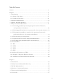

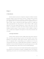
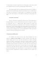

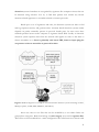


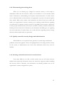

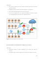

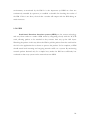


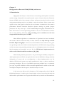
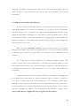
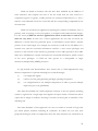
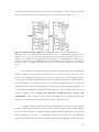
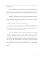
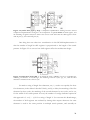
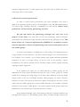
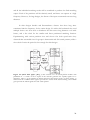
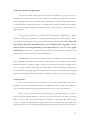
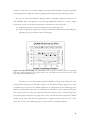


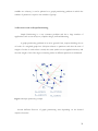
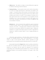
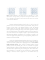
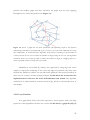
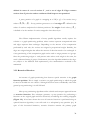
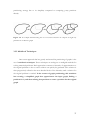
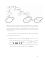
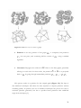
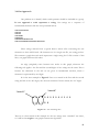
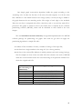
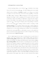
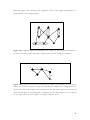
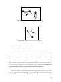
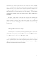
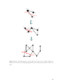
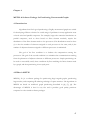
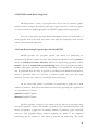
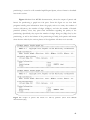
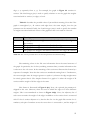
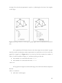


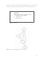
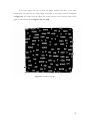
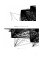
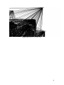

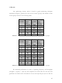

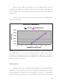
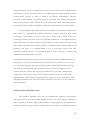


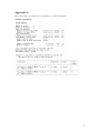

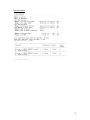
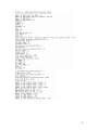
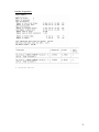
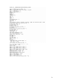
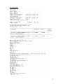


![[U4.23.05] Opérateur DEFI_PARTITION](http://vs1.manualzilla.com/store/data/006359701_1-458a76a27f841754f0d8bab98079b930-150x150.png)

![[U4.23.05] Opérateur DEFI_PART_FETI](http://vs1.manualzilla.com/store/data/006388819_1-f850c452b2fe1c715672e566b583dca9-150x150.png)