1
Class D Audio Amplifier and EQ Iowa State University TI Innovation Challenge 2014 Project Report Spencer Bell ([email protected] or [email protected]) Team Leader: Team Members: Josh Schau ([email protected]) Kyle Shearer ([email protected]) Mackenzie Tope ([email protected]) Seth Weiss ([email protected]) Advising Professor: Dr. Ayman Fayed ([email protected]) Texas Instruments Mentor (if applicable): N/A Date: 5/4/2014 Qty. List all TI analog IC or TI processor part number and URL 13 OPA1662 3 TLV3501 1) Explain where it was used in the project? 2) What specific features or performance made this component well-suited to the design? Low noise: 3.3nV/√Hz Low distortion 0.00006% With very low noise and low distortion, the OPA1662 was used for all op-amps in the circuit that operated with either audio signals or the triangle wave. This included the input buffer, equalizer, triangle wave generator, high gain stage and feedback op-amps. 4.5ns propagation delay Rail to rail outputs With the high speed and rail to rail outputs, the tlv3501 comparator was used to create the PWM signal as well as form the Schmitt trigger for the triangle wave generation circuit. 4 UCC27211 4A source/sink current High & Low side Drivers The UCC27211 gate driver was critical in driving the power MOSFETS fast enough to increase our efficiency and improve the audio quality of the amplifier. 8 CSD18533 60V Vds High current capacity 28nQ Gate Charge The CSD18533 was used in the power amplifier stage of the amplifier. The high voltage and current ratings allowed us to output sufficient power to our speaker. The ultra-low gate charge was essential for fast switching speeds that where needed to keep the efficiency of the amplifier high and the distortion of the amplifier low. 3 LM317HV 60V input voltage Adjustable output voltage The lm317HV was used to create the power rails for the majority of the amplifier circuitry. The high input voltage allowed for each rail voltage to be dependent on just one regulator instead of a cascade of regulators. The ability to easily adjust the voltage allowed us to use the same part for all of the rail voltages needed in the amplifier. 4 SN74LVC1G02 3.6ns propagation delay The SN74LVC1G02 2 input nor gate was used in the non-overlapping clock gating circuit. The low propagation delay was attractive as it allowed to create short dead times in the PWM signals. Spring 2014 Audio Amplifier and 3-‐Band Equalizer 6 SN74LVC2GU04 3.7ns propagation delay The SN74LVCGU04 dual inverter was used in the non-overlapping clocked gating circuit. The low propagation delay was attractive as it allowed to create short dead times in the PWM signals. Submit your TI Innovation Challenge project to TI’s Project repository. Your team is encouraged to post your project as early as possible- Your submission will be kept offline until the contest has officially closed! Instructions: • Project Name must be labelled “TI IC Design Contest North America: Project Name and School” • Fill out project form (template is completely flexible) and include the following documents o The TI report template o Your full class report o Supplemental photos o A video of your partially or fully built out design. We’d love to see your team engaging with TI products! Project abstract (a short high level written description of the design and motivation behind project), 1,000 words max: The project is to design, test, and physically construct a Class D Audio Amplifier. This system must be very efficient and have very low noise, because those are the important characteristics of a good audio amplifier. There are many different types of audio amplifiers, but this project is to build a Class D amplifier. Class D amplification is just a specific type of amplifier that uses a special scheme to amplifier a signal. Our project includes an equalizer so that the user can change the sound of the amplifier. Many audio systems have an equalizer because it allows the user to get a sound that he or she likes, and it allows for customization from the user. The Class D audio amplifier must be at least 80% power efficient, the signal to noise ratio must be at least 96 dBs, and the system must have a 3-‐band equalizer. These are the technical requirements of the project. Other goals we had were to implement a 5-‐band equalizer, make sure the equalizer is user friendly and can adequately change the sound of the amplifier, have a housing case for the entire system and enter in the TI Innovation Challenge competition. Please submit your class report with this one page document. Your class report should include the following (Max of 30 pages, excluding appendix): • Table of contents • List of figures and tables • A detailed written description of the project design • Hardware Design • Any Software Architecture used (include any software code as part of Appendix) • Testing and Results / Conclusions • Future Work / Recommendations • Acknowledgements and/or References • Appendix: schematics, CAD drawings, Critical IC Bill of Materials (Entrants may use Digikey Online BOM tool on www.Digikey.com), User Manual, etc. MAY14-‐02 Page 2 Audio Amplifier and 3-‐Band Equalizer SSQW057 MAY14-‐02 Page 3 Audio Amplifier and 3-‐Band Equalizer CLASS D AMPLIFIER AND 5-BAND EQUALIZER MAY 14-02 Team Members: Spencer Bell Kyle Shearer Josh Schau Seth Weiss Mackenzie Tope Advisor: Ayman Fayed MAY14-‐02 Page 4 Audio Amplifier and 3-‐Band Equalizer Table of Contents 1. Introduction ................................................................................................................................... 8 1.1 Audio Systems .................................................................................................................................... 8 1.2 Requirements ..................................................................................................................................... 8 1.3 Operational Environment ................................................................................................................... 8 2. Design Concept .............................................................................................................................. 8 2.1 Concept Sketch ................................................................................................................................... 8 2.2 Functional Specifications .................................................................................................................... 8 2.3 Qualitative Descriptions ..................................................................................................................... 9 2.3.1 Linear Regulator ........................................................................................................................... 9 2.3.2 Triangle Wave Generator ............................................................................................................. 9 2.3.3 PWM ............................................................................................................................................. 9 2.3.4 Complementary Non-‐overlapping Clock Gate .............................................................................. 9 2.3.5 Drivers .......................................................................................................................................... 9 2.3.6 H Bridge ........................................................................................................................................ 9 2.3.7 Output Filter ................................................................................................................................. 9 2.4 Standards .......................................................................................................................................... 10 2.4.1 Audio Jack ................................................................................................................................... 10 3. System Level Description ........................................................................................................ 10 3.1 Class-‐D Amplifier .............................................................................................................................. 10 3.2 EQ Design .......................................................................................................................................... 11 3.2.1 Simulated Inductors .................................................................................................................... 11 3.2.2 Gain Control ............................................................................................................................... 14 3.2.3 Selecting Band Frequencies ........................................................................................................ 16 3.2.4 “W” Taper Potentiometers ......................................................................................................... 17 3.2.5 Testing ........................................................................................................................................ 18 4. Class D Design ............................................................................................................................. 21 4.1 Speaker Specifications ...................................................................................................................... 21 4.2 Triangle Wave Generator ................................................................................................................. 21 4.4 Non-‐overlapping Clock Gating .......................................................................................................... 23 4.4.1 Why? .......................................................................................................................................... 23 4.4.2 How ............................................................................................................................................ 24 4.4.3 Results ........................................................................................................................................ 24 4.5 Drivers .............................................................................................................................................. 25 4.6 Power Stage ...................................................................................................................................... 27 4.7 Output Filter ..................................................................................................................................... 28 4.8 Feedback ........................................................................................................................................... 29 5. Testing and Evaluation ............................................................................................................ 31 MAY14-‐02 Page 5 Audio Amplifier and 3-‐Band Equalizer 5.1 Power Testing and Analysis .............................................................................................................. 31 5.2 Audio Quality Testing and Evaluation ............................................................................................... 31 5.3 EQ Functionality Testing and Evaluation .......................................................................................... 32 6. Future Considerations ............................................................................................................. 34 6.1 Proffesional PCB ............................................................................................................................... 34 6.2 Second Channel ................................................................................................................................ 34 6.3 Wireless Transmission ...................................................................................................................... 34 6.4 Digital Proccesing ............................................................................................................................. 34 7. Appendix I: Operation Manual .............................................................................................. 35 8. Appendix II: Failed Designs .................................................................................................... 36 8.1 Shoot-‐Through Solutions .................................................................................................................. 36 8.1.1 Offset Triangle Wave .................................................................................................................. 36 8.1.2 Unilateral Delay .......................................................................................................................... 36 8.2 Equalizer Designs .............................................................................................................................. 37 8.2.1 Baxandall .................................................................................................................................... 37 8.2.2 Cascaded Filters .......................................................................................................................... 38 9. Glossary ......................................................................................................................................... 39 Table of Figures FIGURE 2.1 SYSTEM DESCRIPTION ......................................................................................................................................... 8 FIGURE 2.2 TRS AUDIO JACK ............................................................................................................................................. 10 FIGURE 3.1 FUNCTION LEVEL DESCRIPTION ........................................................................................................................... 11 FIGURE 3.2 SIMULATED INDUCTOR ...................................................................................................................................... 11 EQUATION 3.1 ………….. ................................................................................................................................................... 12 EQUATION 3.2…………… ................................................................................................................................................... 12 EQUATION 3.3 ……………….. ............................................................................................................................................. 12 EQUATION 3.4………………… ............................................................................................................................................. 12 EQUATION 3.5…… ........................................................................................................................................................... 12 EQUATION 3.6….. ........................................................................................................................................................... 12 FIGURE 3.3 SIMULATED RLC (LEFT) RLC FILTER (RIGHT) ......................................................................................................... 12 FIGURE 3.4 RLC FILTER (LEFT) SIMULATED RLC (RIGHT) .......................................................................................................... 13 FIGURE 3.5 FREQUENCY RESPONSE OF RLC VS SIMULATED RLC ............................................................................................... 13 FIGURE 3.6 ADJUSTABLE GAIN BAND-‐PASS FILTER ................................................................................................................. 14 EQUATION 3.7 ................................................................................................................................................................ 14 EQUATION 3.8 ................................................................................................................................................................ 14 FIGURE 3.7 ATTENUATING FILER CIRCUIT………… .................................................................................................................. 15 FIGURE 3.8 AMPLIFYING FILTER CIRCUIT…………. ................................................................................................................... 15 EQUATION 3.9 ................................................................................................................................................................ 15 FIGURE 3.9 BAND EQUALIZER CONFIGURATION ..................................................................................................................... 15 TABLE 3.1 FIVE-‐BAND EQUALIZER SPACING .......................................................................................................................... 16 MAY14-‐02 Page 6 Audio Amplifier and 3-‐Band Equalizer TABLE 3.2 FIVE-‐BAND EQUALIZER VALUES ............................................................................................................................ 16 FIGURE 3.10 FIVE BAND EQUALIZER FULL SCHEMATIC ............................................................................................................ 16 FIGURE 3.11 GAIN (DB) VS POTENTIOMETER ROTATION ........................................................................................................ 17 FIGURE 3.12 W-‐TAPER CHARACTERISTICS ............................................................................................................................ 18 FIGURE 3.13 FREQUENCY RESPONSE (HIGH BASS, LOW MIDS, MEDIUM HIGHS) ......................................................................... 19 FIGURE 3.14 ALL POTENTIOMETERS MAXIMUM .................................................................................................................... 19 FIGURE 3.15 ALL POTENTIOMETERS MINIMUM ..................................................................................................................... 20 FIGURE 3.16 EQUAL GAIN ADJUSTMENT .............................................................................................................................. 20 EQUATION 4.1…………………… .......................................................................................................................................... 21 FIGURE 4.1 TYPICAL TRIANGLE WAVE GENERATOR CIRCUIT ..................................................................................................... 21 FIGURE 4.2 TRIANGLE WAVE GENERATOR SCHEMATIC IN USE .................................................................................................. 22 FIGURE 4.3 TRIANGLE WAVE MEASURED IN OSCILLOSCOPE ..................................................................................................... 22 FIGURE 4.4 COMPARATOR ................................................................................................................................................. 23 FIGURE 4.5 NON-‐OVERLAPPING CLOCK GATING CIRCUIT ......................................................................................................... 24 FIGURE 4.6 NON-‐OVERLAPPING CLOCK GATING WAVEFORM ................................................................................................... 25 FIGURE 4.7 NON-‐OVERLAPPING CLOCK GATING DEAD TIME .................................................................................................... 25 FIGURE 4.8 DEAD TIME OF 20NS BETWEEN HIGH SIDE (BLUE) AND LOW SIDE (YELLOW) ............................................................... 26 FIGURE 4.9 GATE DRIVER CONNECTED TO MOSFET .............................................................................................................. 27 FIGURE 4.10 POWER STAGE SCHEMATIC SHOWING H BRIDGE AND OUTPUT FILTER ..................................................................... 27 FIGURE 4.11 OUTPUT FILTER ............................................................................................................................................. 28 FIGURE 4.12 BODE PLOT OUTPUT FILTER ............................................................................................................................. 29 FIGURE 4.13 OUTPUT FILTER RIPPLE ................................................................................................................................... 29 FIGURE 4.14 FEEDBACK CIRCUIT ......................................................................................................................................... 30 FIGURE 4.15 HIGH GAIN STAGE ......................................................................................................................................... 31 FIGURE 5.1 NOISE FLOOR .................................................................................................................................................. 31 FIGURE 5.2 AMPLIFIER CONNECTED TO SPEAKERS .................................................................................................................. 32 FIGURE 5.3 SIDE VIEW .......................................................................................................... ERROR! BOOKMARK NOT DEFINED. FIGURE 5.4 ROUTED PCB .................................................................................................................................................. 32 FIGURE 8.1 ..................................................................................................................................................................... 36 FIGURE 8.2 ..................................................................................................................................................................... 37 FIGURE 8.3 ..................................................................................................................................................................... 37 FIGURE 8.4 ..................................................................................................................................................................... 38 MAY14-‐02 Page 7 Audio Amplifier and 3-‐Band Equalizer 1. INTRODUCTION 1.1 AUDIO SYSTEMS In order to play music from an audio device through speakers, usually there is need of a separate power supply that will drive the speakers because media devices don’t have that kind of power. This is reason for amplifiers. Audio amplifiers take the output from a media device such as an iPod and produce the same signal but at a higher power level capable of driving large speakers. This way very little power is used from the media device. Most audio systems also implement an equalizer that will take signal from the media device and level out a set of frequencies to a desired gain. This allows for users to control the volume levels of the low, middle, or high end frequencies. 1.2 REQUIREMENTS The system is designed to take an audio input from a media device, such as an iPhone, Android, tablet, etc. The explicit Class-‐D amplifier in the system must have a power efficiency of 80%. The system also outputs a waveform that has a signal-‐to-‐noise ratio greater than or equal to 96dB. The system also has a 5-‐band equalizer to adjust frequency bands to the desired amplitudes. 1.3 OPERATIONAL ENVIRONMENT The system must be operable in normal commercial environments. The audio amplifier is designed to be used near humans, so no special consideration need to be made about temperature or other operating conditions. The system will be portable enough for one person to operate and move without significant strain. The system should have measures to ensure it does not bring any hazards to the environment in which it is operating. 2. DESIGN CONCEPT 2.1 CONCEPT SKETCH Figure 2.1 is a basic sketch of the system. The blue blocks represent the system designed and implemented. The red blocks are representations of the devices that can be enhanced by using the class-‐D amplifier. Figure 2.1 System Description 2.2 FUNCTIONAL SPECIFICATIONS MAY14-‐02 Page 8 Audio Amplifier and 3-‐Band Equalizer The requirements set in section 1.2 are specific goals the system has met. The system also accepts different types of media, such as iPods, CD Players, or any type of basic commercial media. Given a media input, the audio amplifier system drives a speaker with more volume than without using any amplification. Speakers have different power ratings and impedance values, so the speakers used in this system are ones that the amplifier can drive. The following is standard in the audio industry: a customer must ensure the speaker and audio amplifier match correctly. The equalizer is 5-‐band, and allows changes the amplitudes of specific frequency content outputted to the speaker. 2.3 QUALITATIVE DESCRIPTIONS 2.3.1 LINEAR REGULATOR With precise required voltage rails of 2.5V, 5V, and 10V, regulators must be used to provide consistent power to the components requiring specific voltages. The linear regulator outputs a constant voltage given sufficient input. 2.3.2 TRIANGLE WAVE GENERATOR In order to amplify a signal properly with a class-‐D amplifier, the signal must first be compared to a triangle wave. This triangle wave is created by integrating a square wave, which originated from a Schmitt Trigger. Following this formation, the triangle wave is amplified by a third operational amplifier to obtain the proper shape required for generating a pulse width modulated signal (PWM). 2.3.3 PWM PWM is accomplished by comparing a signal with a triangle wave. This allows the signal to be amplified very efficiently using a power amplification stage. 2.3.4 COMPLEMENTARY NON-OVERLAPPING CLOCK GATE The power stage consists of two MOSFETs that if not controlled carefully can both be turned on at the same time. This creates a short between the supply voltage rails that wastes a lot of power and produces a very large current called shoot-‐through 2.3.5 DRIVERS Drivers take the PWM signal and drive the power MOSFETS with the same signal. Drivers are needed as they can greatly reduce turn on and off times of the MOSFETS and will reduce switching losses and distortion of the audio signal 2.3.6 H BRIDGE The H bridge consists of a series of power MOSFETS that amplify the power of the PWM signal. This is a crucial portion because all of the amplification is done at this stage. 2.3.7 MAY14-‐02 OUTPUT FILTER Page 9 Audio Amplifier and 3-‐Band Equalizer An LC filter is used immediately after the power stage to recover the original audio signal. It also acts as a filter for the high-‐powered square wave present with the PWM. An LC filter is used as it has no resistive elements and so is very efficient. 2.4 STANDARDS 2.4.1 AUDIO JACK The only relevant standard for our application is the use of a 3.5mm audio jack as an input to the system. The jack most commonly used in devices today is a TRRS (Tip, Ring, Ring, and Sleeve) jack. This jack has four connections. Starting from the tip there is the left channel connection, right channel, ground, and microphone connection. There is a discrepancy with the order of the ground and microphone connections on older devices but most new devices follow ground and then microphone. Figure 2.2 TRS Audio Jack Since our amplifier will not have a microphone on it we will be using a TRS (Tip, Ring, and Sleeve) jack that only has 3 connections; left channel, right channel, ground. 3. SYSTEM LEVEL DESCRIPTION 3.1 CLASS-D AMPLIFIER The class D amplifier is an amplifier design based on the principal of using an audio signal to control a 2 PWM . The PWM is amplified and the audio signal is then recovered using a low pass filter. The switching power MOSFET’s add a similarity between the class D amplifier and a switching mode power supply and so the efficiency of the class D amplifier is very high. The audio signal to be amplified is connected to one of the terminals of a comparator. The other terminal has a high frequency triangle wave pulsing at a constant frequency and amplitude (the triangle waves frequency must be about 15 times greater than the frequency of the signal to be amplified). This creates a digital pulse wave. The width of a pulse is directly related to the audio signals amplitude at that specific time. Due to the high frequency of the triangle wave, the PWM signal acts as a digital sample of the audio signal. Afterward the pulse wave modulated signal is connected to a gate-‐driver, to help drive the next stage. This stage is a push-‐pull power MOSFET configuration. When the inputted digital pulse wave arrives at the gates of the MOSFETs, the push pull network amplifies the signal. When the digital pulse signal values at high, the PUN MOSFET puts VDD as the output. When the digital pulse signal is low, the PDN MOSFET pushes the signal to Vss. This effectively is a digital signal amplifier, whose gain is related to MAY14-‐02 Page 10 Audio Amplifier and 3-‐Band Equalizer the difference between Vdd and Vss. This digital signal is then put through a low pass filter to attenuate the high frequency PWM and pass the audio signal components. The resulting signal is sent to the speaker. Figure 3.1 Function Level Description 3.2 EQ DESIGN 3.2.1 SIMULATED INDUCTORS Our equalizer design consists of 5, constant quality factor (frequently called "Constant Q"), band-‐ pass filters controlled by 5 individual potentiometers. The design relies heavily on the use of "simulated inductors" for its frequency shaping characteristics. It's no secret that inductors have tremendous frequency shaping capabilities when combined with capacitors and resistors, but inductors are bulky, expensive and difficult to find in precise values. Luckily, the characteristics of an inductor can be realized using an op amp, two resistors and a capacitor as shown in the circuit below. Figure 3.2 Simulated Inductor MAY14-‐02 Page 11 Audio Amplifier and 3-‐Band Equalizer The circuit in Figure 3.2 works by basically reversing the operation of a capacitor, thus artificially simulating an inductor. The following equations relate the RLC band-‐pass filter in Figure 3.3 (right) to the simulated RLC band-‐pass filter in Figure 3.3 (left). 𝒇𝟎 = 𝑸= 𝟏 𝟐𝝅∗ 𝑳𝑪𝟐 𝟐𝝅∗𝒇𝟎 ∗𝑳 𝐵𝑊 = 𝑹𝟐 !! ! Equation 3.2 Equation 3.4 Equation 3.6 Equation 3.1 𝑳 = 𝑹𝟏 − 𝑹𝟐 ∗ 𝑹𝟐 ∗ 𝑪𝟏 Equation 3.3 𝑪𝟏 = 𝟐𝝅∗𝒇 Equation 3.5 𝐶! = !!∗! ∗! 𝑸 𝟎 ∗(𝑹𝟏 !𝑹𝟐 ) ! ! ! ∗! *note: the quality factor "Q" refers to the ratio between the center frequency "ƒo" and the -‐3dB bandwidth "BW". Figure 3.3 Simulated RLC (left) RLC Filter (right) For example, if an RLC band-‐pass filter with a center frequency (ƒ0) of 1KHz and a quality factor (Q) of .85 is desired, R2 can be chosen freely and the values of L and C2 can be calculated using Equations 3.1 and 3.3. With R2 and C2 known, the equivalent band-‐pass filter utilizing a simulated inductor can be calculated using Equations 3.2, 3.4, and 3.6. Figure 3.4 shows one possible pair of a solution. MAY14-‐02 Page 12 Audio Amplifier and 3-‐Band Equalizer Figure 3.4 RLC filter (left) Simulated RLC (right) Running a frequency sweep from 20Hz to 20KHz on both circuits produces the following plot in Figure 3.5. While it's difficult to see, what appears to be a single output is actually one output lying almost perfectly on top of the other. Now, with the ability to build a precise and inexpensive filter, the question becomes how to arrange five band-‐pass filters to make a fully functional and user-‐ friendly equalizer. Figure 3.5 Frequency Response of RLC VS Simulated RLC MAY14-‐02 Page 13 Audio Amplifier and 3-‐Band Equalizer 3.2.2 GAIN CONTROL To give the user the ability to adjust the gain of the band-‐pass filter, we used the configuration in Figure 3.6. Figure 3.6 Adjustable Gain Band-‐Pass Filter In this circuit, when the potentiometer is rotated to its most counter-‐clockwise position (0%), R4 drops out of the gain equation and the circuit effectively becomes an attenuator for that particular frequency band where the gain equation is given by Equation 3.7 below. The equivalent circuit that results is shown in Figure 3.7. When the potentiometer is rotated to its most clockwise position (100%), R3 drops out of the equation and the circuit becomes an amplifier where the gain is given according to Equation 3.8. The equivalent circuit is show in Figure 3.8. With the potentiometer at 50%, the amplification cancels out the attenuation and a unity gain buffer is created (A=1). When the potentiometer lies between the 0%, 50% and 100% marks, a combination of attenuation and amplification takes place resulting in partial attenuation or amplification. 𝑨= 𝑹𝟐 𝑹𝟐 + 𝑹𝟑 Equation 3.7 𝑨= 𝑹𝟒 + 𝟏 𝑹𝟐 Equation 3.8 MAY14-‐02 Page 14 Audio Amplifier and 3-‐Band Equalizer Figure 3.7 Attenuating Filer Circuit Figure 3.8 Amplifying Filter Circuit From looking at Equation 3.7 and Equation 3.8 it becomes clear that the gain boundaries of the filter are dictated by the ratio of R3 and R4 to R2. We want to give the user the ability to adjust the output to anywhere between -‐17dB and 17dB (decibels) for each band so using Equation 3.7, Equation 3.8, and Equation 3.9 to realize these gains at 0% and 100% potentiometer rotation the ratio of R4 to R2 has to equal about 7:1 and R3 must equal R4. Choosing R3 and R4 to equal 3.3KΩ and setting R2 to 470Ω for all filters gives us the desired result. 𝐺𝑎𝑖𝑛 𝑑𝐵 = 20 ∗ log (𝐴) Equation 3.9 For a 5-‐band equalizer the circuit will be constructed as shown in Figure 3.9. Figure 3.9 Band Equalizer Configuration Simply by paralleling the potentiometers of each filter across the inverting and non-‐inverting terminals of the op amp shown at the top right of Figure 3.9, an equalizer with virtually any number of bands can be constructed. The difficult part becomes deciding which frequencies to assign to each filter to maximize performance and tonal coherence. MAY14-‐02 Page 15 Audio Amplifier and 3-‐Band Equalizer 3.2.3 SELECTING BAND FREQUENCIES Because humans hear pitch logarithmically, building an equalizer with filters that are evenly spaced on the frequency spectrum tends to produce changes in pitch that sound disjointed when amplified or attenuated. The solution to this is to space the filters out logarithmically as well. However, while music is very mathematical, it's also very subjective. Defining something as sounding "good" is not universal so experimentation and trial and error tends to be a very important part of sound design. While keeping Q constant and testing different combinations of filters to see how they affected one another, we settled on spacing out our filters in a semi-‐logarithmic fashion as shown in Table 3.1. Band 1 Band 2 Band 3 Band 4 Band 5 Frequency 60Hz 250Hz 1KHz 4KHz 16KHz Q Factor 0.85 0.85 0.85 0.85 0.85 Table 3.1 Five-‐Band Equalizer Spacing With the center frequencies, Q factor and gain ratio resistor values known, the remaining components can be solved for utilizing equations 3.2, 3.4 and 3.6. The component list and full circuit design are shown in Table 3.2 and Figure 3.10 respectively. 60Hz 250Hz 1KHz 4KHz 16KHz C1 180nF 4.7nF 5.1nF 2.7nF 2.7nF C2 6.6uF 1.59uF 398.2nF 100nF 24.8nF R1 13KΩ 12KΩ 27KΩ 13KΩ 3.6KΩ R2 470Ω 470Ω 470Ω 470Ω 470Ω Table 3.2 Five-‐Band Equalizer Values Figure 3.10 Five Band Equalizer Full Schematic MAY14-‐02 Page 16 Audio Amplifier and 3-‐Band Equalizer Note that in the above schematic, a buffer amplifier separates the music source from the equalizer so the needed currents are drawn from the buffer stage rather than the music device. Hooking a music device directly to the equalizer input would drain the device very quickly and could cause permanent damage. Also note that decoupling capacitors have been placed in strategic locations around the circuit to limit rail noise. 3.2.4 “W” TAPER POTENTIOMETERS One issue inherent with this equalizer design is the nonlinearity of the gain versus potentiometer rotation when using linear potentiometers. Because of the way the two gain equations interact with each other when the pots are between extremes, a reverse "S" shaped curve forms as the potentiometers travel from 0% to 100% rotation as shown in Figure 3.10. The result is a series of potentiometers that have almost no perceivable effect on the circuit with the exception of the first and last 5% of rotation. This makes it incredibly difficult for the user to subtly adjust tones to suit their liking. Gain (dB) 20 15 Gain (dB) 10 5 0 -‐5 0% 10% 20% 30% 40% 50% 60% 70% 80% 90% 100% -‐10 -‐15 -‐20 % Pot Rota_on Figure 3.11 Gain (dB) VS Potentiometer Rotation To solve this problem we used "W-‐taper" potentiometers to counteract the reversed S-‐shaped curve of the equalizer's gain characteristics. A graph of gain versus pot rotation is shown below in Figure 3.12. The W-‐taper potentiometer's output characteristics are exactly opposite of the equalizer's natural gain characteristics. By replacing the standard linear potentiometers with new W-‐taper pots, the resulting gain outputs are effectively linearized. MAY14-‐02 Page 17 Audio Amplifier and 3-‐Band Equalizer Figure 3.12 W-‐Taper Characteristics 3.2.5 TESTING Testing was carried out both physically and virtually. Circuit simulation software proved to be a valuable resource when building and modifying the filter designs. Below are some examples of equalizer's output under various band adjustments. The solid, black line depicts the output of the equalizer in each case. In Figure 3.13, the bass pots (60Hz and 250Hz) and treble pots (4KHz 16KHz) are set high with the mid pot (1KHz) set to its minimum value. The band overlap keeps each filter from achieving its full gain potential in the output but the frequency response is still reasonable. Qualitatively, it sounds very good. Figure 3.14 and Figure 3.15 depict the output of the equalizer when all potentiometers are at their extremes. In the case of Figure 3.14, all pots are at maximum and in Figure 3.15 all pots are at minimum. As is the case in both instances, with all pots at their extreme values, a 3dB ripple occurs caused by an increased Q factor. Since Equalizers are for shaping sound and not amplifying all frequencies, it's not anticipated that this characteristic would bother the end user. If the user wants their sound louder, they need to increase the volume on the amplifier, not the equalizer. MAY14-‐02 Page 18 Audio Amplifier and 3-‐Band Equalizer Figure 3.13 Frequency Response (High Bass, Low Mids, Medium Highs) Figure 3.14 All Potentiometers Maximum MAY14-‐02 Page 19 Audio Amplifier and 3-‐Band Equalizer Figure 3.15 All Potentiometers Minimum Figure 3.16 Equal Gain Adjustment MAY14-‐02 Page 20 Audio Amplifier and 3-‐Band Equalizer Figure 3.16 paints a good picture of how the equalizer's performance changes with an equal increase in pot rotation. At low gains the output is very uniform and as the gains of each band increase the development of the 3dB ripple becomes more and more prominent. 4. CLASS D DESIGN 4.1 SPEAKER SPECIFICATIONS For our system we will use two speaker systems, one for each channel, that each have an impedance of 4 ohms. Each speaker set should also be rated for 250 W RMS to handle the full power of the amplifier. Each speaker set should contain multiple speakers with their own crossover. 4.2 TRIANGLE WAVE GENERATOR In order to amplify a signal properly with a class-‐D amplifier, the signal must first be compared to a triangle wave. This triangle wave is created by integrating and amplifying a square wave using four operational amplifiers-‐-‐two in series, two in parallel (see figure 4.2b). The triangle wave generator was designed by combining a Schmitt trigger and a Miller integrator. Figure 4.1 details the schematic. The frequency of the triangle wave generator was needed to be close to 300 kHz and the resulting equation for finding the component values is as follows. 𝑹 𝒇𝒐𝒖𝒕 = 𝟒𝑹 𝑹𝟐 𝑪 𝒕 𝟏 Equation 4.1 The amplitude of the triangle wave is determined by the ratio of R1/R2. Figure 4.1 Typical Triangle Wave Generator Circuit The values of the components were found as R1 = 1Kohm, R2 = 6Kohm, Rt = 500ohm, C = 5nf. It was 3 found that the op amp used in the Miller integrator had a large impact on the quality of the wave and so an opa1662 precision op amp was used to create a consistently accurate triangle wave. Figure 4.2 details the schematic with component values. MAY14-‐02 Page 21 Audio Amplifier and 3-‐Band Equalizer Figure 4.2 Triangle Wave Generator Schematic in Use The resulting output triangle wave has a frequency of 290 KHz and amplitude of 4 Volts with a power supply of +-‐ 5 Volts. Figure 4.3 Triangle Wave Measured in Oscilloscope 4.3 PWM Pulse Width Modulation (PWM) was used to encode the audio signal in a way that could be very efficiently amplified in a later stage. To create the PWM, the audio signal from the equalizer was compared to the triangle wave. This modulation works by linearly encoding the amplitude of the audio wave to the width of the PWM. The straight-‐line shape is why a triangle wave was used but other waves consisting of linear changes in amplitude through time could have been used. To ensure high quality, a high speed TLV3501 comparator was used to create a PMW. MAY14-‐02 Page 22 Audio Amplifier and 3-‐Band Equalizer Figure 4.4 Comparator 4.4 NON-OVERLAPPING CLOCK GATING 4.4.1 WHY? A non-‐overlapping clock system is needed to prevent the power MOSFETS from turning on at the same time. In the original design the two MOSFETS on one side of the bridge were controlled by the same signal just inversed. That way when the high side MOSFET would turn on the low side MOSFET would be turning off at the same time. The problem though is that the switch doesn’t happen instantaneously. There is a brief moment when the signals are switching that the MOSFETS will both be on at the same time. When this happens there is a connection between the rail voltages with very little resistance. High voltages and low resistance mean high current. High current means heat and power loss. A delay is introduced to prevent this and will give the signals time to switch. MAY14-‐02 Page 23 Audio Amplifier and 3-‐Band Equalizer 4.4.2 HOW Figure 4.5 Non-‐Overlapping Clock Gating Circuit Figure 4.5 shows the non-‐overlapping clock circuit. The circuit has two NOR gates connected to the output of the opposing side. To understand how this works it is easiest to walk through the signal changes step by step. At a steady state when the PWM is high the bottom NOR gate will have two high signals at the input and therefore a low output at the gate and at the final output as well. The top NOR gate will have two low signals at the input and therefore a high output at the gate and the final output. Now when the PWM switches to low, the signal at the top NOR gate will have a high and a low input therefore changing its output to low but at that instant the bottom gate will also have a high and low input so it will still output low. Once the signal change in the top propagates through the inverters the output at the top changes to low. Only then will the NOR gate receive two low signals allowing it to output high and propagate a high on the final output. This design will always put a delay on the rising edge of each output giving just enough time for the one MOSFET to turn off before the other one turns on. 4.4.3 RESULTS Figure 4.6 shows two waveforms, one for the high side gate driver and one for the low side gate driver. These waveforms came from measuring the output of the circuit built from Figure 4.5. It is easy to see that the signals are never high at the same time. Figure 4.7 shows a closer look at the dead time between switches. The dead time is the amount of time that both MOSFETs are off. MAY14-‐02 Page 24 Audio Amplifier and 3-‐Band Equalizer Figure 4.6 Non-‐Overlapping Clock Gating Waveform Figure 4.7 Non-‐Overlapping Clock Gating Dead Time The turn on voltage for our MOSFETS is ~3V. So in order to measure the dead time we had to measure the time when the falling edge for one side dropped below 3V and the rising edge for the other rose above 3V. Figure 4.7 shows that time to be ~20 ns. 4.5 DRIVERS Drivers are a components that can turn MOSFETs on and off at high speeds by providing high current pulses. Suitable drivers are crucial because the performance of class d amplifier is directly related to the MAY14-‐02 Page 25 Audio Amplifier and 3-‐Band Equalizer speed at which the power MOSFETs can be switched on and off. This is due to a tradeoff between switching losses and audio quality. Switching losses occur when a transition in the half bride is made by turning one MOSFET on and another off. During this transition both power MOSFETs can be turned on for a short time. This creates a short from 48V to ground that causes a large current spike known as shoot-‐through. A pause known as dead time is added between the switching times of the high and low side MOSFETs to tackle shoot-‐through. Switching losses also occur when turning the high side power MOSFET on and the low side power MOSFET off. When the high side MOSFET switches on, the drain of the low side power MOSFET increases from 0 volts to 48 volts. Gate to drain capacitances in the low side MOSFET pass through some charge during the transition, which in turn increases the voltage on the gate of the low side MOSFET. If too much charge is passed through to the gate of the low side MOSFET, the MOSFET can be turned on causing a large amount of shoot-‐through. Including a dead time between the switching of the low and high side power MOSFETs leaves a period when neither of the MOSFETs are conducting. During this time the inductor in the output filter is not provided with the true PWM signal. This leads to distortion of the audio signal. A high fidelity amplifier will need very short dead times so as to cause as little distortion as possible. A variety of different dead times were tried but best results were found when using 20ns. Dead times longer than 20ns did not improve on the switching losses and THD was within inaudible limits. Figure 4.8 Dead Time of 20ns Between High Side (blue) and Low Side (yellow) The driver chosen was the UCC27211. The UCC27211 is capable of driving a full half bridge with the addition of a bootstrap capacitor. It is able to source and sink 4A of current to the gates of the power MOSFETs that can turn them off and on in 7ns. MAY14-‐02 Page 26 Audio Amplifier and 3-‐Band Equalizer Figure 4.9 Gate Driver Connected to MOSFET The power losses per channel where measured to be 9W, which is 2% of the maximum rated output power of 500W. This loss doubles to 4% when stereo is implemented. This loss was primarily due to switching losses. 4.6 POWER STAGE To increase the power of the PWM signal a MOSFET H bridge was implemented. The H Bridge consists of two pairs of n channel MOSFETs that end up driving both sides of the speaker. The advantage of the H bridge is that it allows for the full supply voltage to be deliverable across the speaker which increases the maximum output power by a factor of four compared to a half bridge topology. Figure 4.10 Power Stage Schematic Showing H Bridge and Output Filter MAY14-‐02 Page 27 Audio Amplifier and 3-‐Band Equalizer For a highly efficient system the MOSFETs had to be carefully chosen to have low gate capacitances and low on resistances. It was decided to choose the MOSFET with the lowest gate capacitance available to reduce switching losses as much as possible as most of the amplifiers pin efficiencies where due to switching losses. The CSD1853KCS was chosen, as it possesses a very low gate capacitance at (3nF) and a low on resistance (4mΩ). 4.7 OUTPUT FILTER The output filter is used means to reduce EMI and increase the longevity of the speaker. This is achieved by filtering the signal produced by the power stage which is a 48V square wave using an LC filter, which consists of an inductor and a capacitor. An LC filter was used, as it theoretically contains no resistive elements meaning an LC filter consumes almost no power. Another advantage of an LC filter is that it contains two poles that cause a decay of -‐40dB after the cut off frequency The values of the output filter where important to calculate as the filter needed to pass the audio spectrum but filter out the 300 KHz square wave. LC filters can also have a resonate frequency which creates a spike in the frequency response just before the cutoff frequency. The desired characteristics of the output filter where to have a cutoff frequency of 30 KHz and a Q factor of 0.707. This would provide a pass band with no ripple and an attenuation of close to -‐40dB to the 300KHz square wave. Figure 4.11 Output Filter To find the ideal values for the inductors and capacitors the following equations where used 𝐿= 𝑅!"#$%#& 4𝜋𝑓!"#$%% 𝐿 = 10.6𝑢𝐻 𝐶= 1 2𝜋𝑓!"#$%% ! ∗ 2𝐿 𝐶 = 1.3𝑢𝐹 These values could not fully be realized so L was rounded down to 10𝑢𝐻 and C was rounded downto 1𝑢𝐹. These values gave a Q factor of 0.63. The cutoff frequency was also increased slightly to 43 KHz and attenuation of -‐34 dB was seen at 300 KHz. MAY14-‐02 Page 28 Audio Amplifier and 3-‐Band Equalizer Figure 4.12 Bode Plot Output Filter When tested the ripple from the output filter had an amplitude of 800mVwhich is an attenuation o -‐35.6dB. Figure 4.13 Output Filter Ripple 4.8 FEEDBACK Negative feedback was implemented to eliminate any dc-‐offset voltage across the speaker as well as to reduce distortion. Feedback was taken from across the speaker terminals using an instrumental amplifier topology and fed back into a high gain stage. MAY14-‐02 Page 29 Audio Amplifier and 3-‐Band Equalizer Figure 4.14 Feedback Circuit Ideally a very large open loop gain could be implemented as it allows for stronger correction when negative feedback is implemented. This strong error correction reduces distortion and some noise caused by other elements in the amplifier. The larger the open loop gain of the amplifier the lower the overall distortion is. As the output filter was a two-‐pole system, it was important to consider the other poles present in the amplifier as well as the open loop gain so that the phase margin was kept above 70 . The high gain stage was implemented using an op-‐amp with a gain bandwidth of 22MHz. It was decided that the open loop gain should be kept low enough so that the bandwidth of the high gain stage was considerably higher than the cutoff frequency of the output filter. This ensures that any phase shift produced by the op-‐amp would not cause the amplifier to be unstable. To determine the open loop gain, the phase response of the output filter was examined to find the phase of 90 degrees. The attenuation caused by the output filter was then examined to be -‐26dB. To create an overall phase margin of 90 the high gain stage was given a gain of 26dB to counteract the attenuation of the output filter. MAY14-‐02 Page 30 Audio Amplifier and 3-‐Band Equalizer Figure 4.15 High Gain Stage 5. TESTING AND EVALUATION 5.1 POWER TESTING AND ANALYSIS A single channel draws 300mA at 48V, which results in a power usage of 14.5W. Which comes to 2.9% of the maximum output power. With the addition of the second channel the power losses come to 5.8%. Copper losses due to inductor resistances and MOSFET on voltages come to 1.5%. This puts the efficiency of the amplifier as a whole at 93%. 5.2 AUDIO QUALITY TESTING AND EVALUATION The current audio quality test shows THD to be at 1%. SNR is hard to distinguish as the oscilloscopes used for testing do not show a noise floor below -‐60dB and so the true SNR cannot be truly measured. Figure 5.1 Noise Floor MAY14-‐02 Page 31 Audio Amplifier and 3-‐Band Equalizer 5.3 EQ FUNCTIONALITY TESTING AND EVALUATION Sine waves were inputted at the corner frequencies of the EQ to verify the corner frequencies were in the correct location. Qualitative testing was done in the form of a sample audio input and sound verification to confirm that the high, middle, and low frequencies were adjustable as expected. Figure 5.2 Routed PCB Figure 5.3 Amplifier Connected to Speakers MAY14-‐02 Page 32 Audio Amplifier and 3-‐Band Equalizer Figure 4 Enclosure Front View Figure 5 Enclosure Inside View MAY14-‐02 Page 33 Audio Amplifier and 3-‐Band Equalizer 6. FUTURE CONSIDERATIONS 6.1 PROFFESIONAL PCB Currently the board on which the amplifier and equalizer are mounted on is a copper board that we had routed at school. Due to time constraints we were unable to order a professional PCB with solder resist and a silk screen. Using a professionally made PCB would have made our work a lot easier when actually mounting the components. We had issues with shorts and bad connections with the current board but a board with proper routing and a good solder resist layer would solve most of the problems we ran into. 6.2 SECOND CHANNEL Again due to time constraints only one channel was implemented. A second channel would be ideal because most media devices output sound in stereo mode, which has one channel for the left speaker and one for the right speaker. 6.3 WIRELESS TRANSMISSION Wireless audio transmission is becoming easier and easier to implement each year and with that it also becomes more commonplace. It is hard to find an audio system these days that doesn’t have some sort of Bluetooth or wireless audio connection. In the beginning we had made a list of additions we would like to add to the amplifier if we had enough time. Wireless transmission was on the list. In reality it wouldn’t have been too hard to implement a Bluetooth connection to the amplifier. A lot of manufacturers sell Bluetooth modules that can be configured and attached to a PCB. Most modules that we briefly researched come equipped to be directly connected to speakers and only require power. However, in order to configure it more serial connections would be needed and a USB port would be needed on the board as well. 6.4 DIGITAL PROCCESING The basis of our design was built on using analog components. However about hallway through the project when we were researching potentiometers for the equalizer we stumbled upon digital pots. We found that they would solve our problem with the linearization of the frequency band gains. While we were researching this we also realized that the majority of our components could be replaced by a microprocessor. This microprocessor would be able to handle the equalization, PWM, and the non-‐ overlapping clock gating. If we were to try and commercialize an amplifier this would be the route we would take because it is way cheaper and less problem prone. MAY14-‐02 Page 34 Audio Amplifier and 3-‐Band Equalizer 7. APPENDIX I: OPERATION MANUAL MAY14-‐02 Page 35 Audio Amplifier and 3-‐Band Equalizer 8. APPENDIX II: FAILED DESIGNS 8.1 SHOOT-THROUGH SOLUTIONS 8.1.1 OFFSET TRIANGLE WAVE Figure 8.1 This circuit, in an attempt to resolve shoot through current, created two triangle waves that were offset from one another. These triangle waves would then be used to create two non-‐overlapping PWM signals that would have an inherit dead time. The circuit added too many extra components and did not accurately produce a short dead time. 8.1.2 UNILATERAL DELAY This circuit worked by creating a one-‐way delay on one edge of the PWM signal. This created two signals that would not overlap due to each PWM signal being delayed on one side. The circuit was not used due to the loading effects from the drivers causing PWM Out1 and PWM Out 2 to overlap at the edges. This overlapping caused shoot-‐through current, therefore invalidating the circuit itself. MAY14-‐02 Page 36 Audio Amplifier and 3-‐Band Equalizer Figure 8.2 8.2 EQUALIZER DESIGNS 8.2.1 BAXANDALL This circuit worked by summing together three different filter circuits that were adjustable by a potentiometer. It was desirable as it only used one op-‐amp and very few components. Figure 8.3 A sharper frequency response was required that this circuit did not provide. The circuit also shifted the cutoff frequencies as each potentiometer was adjusted, which is an axiomatic problem. MAY14-‐02 Page 37 Audio Amplifier and 3-‐Band Equalizer 8.2.2 CASCADED FILTERS The cascaded equalizer design had the proper frequency responses when tentative adjustments were made to each potentiometer. Despite this, frequency bands behaved sporadically when approaching maximums and minimums. Audio signals passing through also exhibited excess noise, producing undesirable output. Figure 8.4 MAY14-‐02 Page 38 Audio Amplifier and 3-‐Band Equalizer 9. GLOSSARY 1. Crossover The sole purpose of a crossover is to split one signal into different frequency bands. A crossover is usually used for a set of speakers where certain speakers, such as a bass speaker, can only handle a select range of frequencies. 2. PWM Pulse Width Modulation (PWM) is the process of altering the pulses that make up a square wave. Specifically the widths of the pulses relative to the square wave’s period is changed in PWM. 3. OP AMP An OP AMP is a device that compares the difference between two voltages and amplifies the difference by a very large amount. OP AMPS are often used in conjunction with negative feedback which allows them to behave as amplifiers with very accurate and linear gains. 4. Slew rate The fasted speed at which an electronic device can change its output voltage. Slew rate is usually measured in volts per microsecond (V/us). MAY14-‐02 Page 39