Download Manual Manual for CN2 version 6.1

Manual
Manual for CN2 version 6.1
Robin Boswell
The Turing Institute Limited
TI/P2154/RAB/4/1.5
January 1990
Task
Document type
Status
Classication
Document class
Int. Doc. ID
Distribution
:
:
:
:
:
:
:
T
Manual
Draft
Public
ITM
TI/MLT/4.0T/RAB/1.2
Universal
Abstract
This document is an introduction and user's manual for release 6.1 of the ruleinduction program cn2.
1
Contents
1 Introduction
4
2 Overview
4
3 Example and Attribute Files
5
3.1 Files
: : : : : : : : : : : : : : : : : : : : : : : : : : : : : : : : : : : :
3.2 Attributes
: : : : : : : : : : : : : : : : : : : : : : : : : : : : : : : : :
3.2.1 Semantics
: : : : : : : : : : : : : : : : : : : : : : : : : : : : :
3.2.2 Attribute ordering
: : : : : : : : : : : : : : : : : : : : : : : : : : : : : : :
7
: : : : : : : : : : : : : : : : : : : : : : : : : : : : : : : : :
9
3.3.2 Syntax
: : : : : : : : : : : : : : : : : : : : : : : : : : : : :
9
: : : : : : : : : : : : : : : : : : : : : : : : : : : : : : :
10
3.4 Specimen input le
: : : : : : : : : : : : : : : : : : : : : : : : : : : :
4 Rules: les and evaluation
10
11
: : : : : : : : : : : : : : : : : : : : : : : : : : : : : : : :
4.2 Class distributions
11
: : : : : : : : : : : : : : : : : : : : : : : : : : : :
12
: : : : : : : : : : : : : : : : : : : : : : : : : : : :
12
: : : : : : : : : : : : : : : : : : : : : : : : : : : : : : : : :
13
4.2.1 Rare classes
4.3 Evaluation
6
7
3.3.1 Semantics
4.1 File format
6
: : : : : : : : : : : : : : : : : : : : : : : :
3.2.3 Syntax
3.3 Examples
5
4.3.1 \All" rule evaluation
: : : : : : : : : : : : : : : : : : : : : : :
4.3.2 \Individual" rule evaluation
2
: : : : : : : : : : : : : : : : : : :
13
14
4.4 Inducing and testing rules
: : : : : : : : : : : : : : : : : : : : : : : :
5 Using CN
5.1 Interactive use
14
15
: : : : : : : : : : : : : : : : : : : : : : : : : : : : : : :
5.1.1 Top-level commands
5.2 Non-interactive use
15
: : : : : : : : : : : : : : : : : : : : : : :
16
: : : : : : : : : : : : : : : : : : : : : : : : : : : :
18
A Getting Started
19
B Example run
19
C Handling of Unknowns and Don't Cares
22
C.1 Training (Learning) Phase
: : : : : : : : : : : : : : : : : : : : : : : :
22
C.2 Testing (Execution) Phase
: : : : : : : : : : : : : : : : : : : : : : : :
22
3
1 Introduction
The program described in this manual is version 6.1 of the Turing Institute's implementation of cn2. For details of the cn2 algorithm itself, and plans for further work,
see [Clark, 1989].
For brevity, I shall use the term \cn2" in the following account to refer both to the
algorithm and to its current implementation.
2 Overview
For instructions on installing cn2, see Appendix xA.
cn2 is a rule-induction program which takes a set of examples (vectors of attribute-
values), and generates a set of rules for classifying them. It also allows you to evaluate
the accuracy of a set of rules (in terms of a set of pre-classied examples).
To use the program, you must provide an ASCII le of examples in a standard format
(described in x 3). When the program has induced some rules from these examples,
you may display or evaluate them, or store them in a le. Rules are stored in a humanreadable form, but they may also be read back in by cn2, to save re-calculating them.
If you have data les in MLT CKRL format, then these can be converted into cn2's
format by a CKRL translator (provided by the Turing Institute). In addition, cn2
can itself translate attributes, examples and decision-trees into CKRL format (see
the Ckrl command in section 5.1.1).
See Appendix xB for an example of a terminal session with cn2.
The interface to cn2 is similar to that for the Turing Institute's other recentlydeveloped program NewID described in [Boswell, 1990], so if you are using both
programs, you may nd the following comparisons useful:
Input The format of attribute and example les is identical for the two programs.
(Declarations of attributes as `binary' are meaningful only for NewID: such declarations will be silently ignored by cn2.)
Commands The interfaces are similar, but NewID has a smaller menu of commands
than cn2, because it has fewer customisable parameters (such as `signicance
4
threshold').
Output The output formats dier (as do the algorithms): cn2 generates production
rules and NewID generates decision trees.
3 Example and Attribute Files
The input to cn2 consists of:
1. A set of attribute declarations.
2. A set of examples.
Items 1. and 2. may be presented in the same le, or in two dierent les. Storing
the attributes separately from the examples makes it possible to read and process
several example les in succession without having to re-load the attribute declarations
(provided all the examples use the same attributes).
3.1 Files
Input les are of three types:
1. Attribute les.
2. Examples les.
3. Attribute and Example les.
The most complex of these, the attribute and example le, consists of a header,
followed by attribute declarations, then examples. The two types of data are separated
by punctuation, as specied in x 3.2.3. (See x 3.4 for a specimen of such a le).
Attribute and example les consist of the appropriate header followed respectively by
attributes and examples.
In all le types, characters between a `%' and the next end-of-line are regarded as
comments and ignored.
5
Formally:
attribute-and-example-le ::=
att-and-ex-header attribute-delarations separator examples
att-and-ex-header ::=
\ATTRIBUTE AND EXAMPLE FILE"
separator ::=
\@"
separator
attribute-le ::=
att-header attributes
att-header ::=
\ATTRIBUTE FILE"
example-le ::=
ex-header examples
ex-header ::=
\EXAMPLE FILE"
The format for attributes and examples in the above grammar is dened below.
3.2 Attributes
3.2.1 Semantics
Attributes are of two types: discrete and ordered. A discrete attribute takes one of
a nite set of values (and the set of values has no further structure). An ordered
attribute takes numeric values: integer or oating point.
An attribute declaration consists of the name of the attribute, together with either:
Its possible values (for a discrete attribute), or
Its numeric type (for an ordered attribute).
For the purposes of the rule-induction algorithm, one of the attributes is distinguished
as the class attribute. The aim of the algorithm is to nd rules whereby the class
6
attribute of an example may be inferred from the non-class attributes. The class
attribute must be discrete.
3.2.2 Attribute ordering
In some domains, it may be desirable to impose constraints on the order in which
attributes are tested. For example, one should determine whether a patient is female
before asking whether she is pregnant, rather than afterwards. Such constraints may
be imposed on cn2 by means of attribute ordering declarations, which (optionally)
follow the attribute declarations.
Note that it is not possible to make the result of one attribute test a precondition of
some other test (for example, \if sex is male, then don't ask about pregnancy") but
given sensible data, an inappropriate test will yield a low entropy gain, and so be
excluded anyway by cn2's existing criteria.
An attribute ordering declaration takes the form:
Attribute1 BEFORE Attribute2;
You may include as many such declarations as you wish. Note that cn2 does not
currently check for \loops" (A before B before C before A ): if you introduce such
a loop, the result will be that none of the attributes involved will ever be used.
:::
Finally, note that the order in which attribute tests are displayed in cn2's output
has no signicance (as it happens, it matches the order of attribute declaration), so
in particular is not aected by attribute ordering constraints. The only eect of, for
example, the constraint sex BEFORE pregnancy is to ensure that any rule containing
a test of pregnancy also contains a test of sex.
3.2.3 Syntax
An attribute declaration consists of the attribute's name, followed either by its possible values (if it's discrete), or its numeric type (if it's ordered), separated by appropriate punctuation. The class attribute must be declared last. (i.e. cn2 will treat the
last attribute as the class attribute).
Formally:
7
attribute-data ::=
attribute-declarations att-ordering-section
j attribute-declarations
attribute-declarations ::=
attribute-declaration
j attribute-declarations attribute-declaration
attribute-declaration ::=
string \:" attribute-values \;"
j string \:" \(" type \)"
% For discrete attributes
% For ordered attributes
attribute-values ::=
string attribute-values
j string
type ::=
\FLOAT"
j \INT"
string ::=
quoted-string
j unquoted-string
att-orderings-section ::=
\ORDERINGS" attribute-orderings
attribute-orderings ::=
attribute-ordering
j attribute-orderings attribute-ordering
attribute-ordering ::=
string \BEFORE" string \;"
An unquoted-string is a sequence of one or more characters made up of
upper or lower-case letters, digits, and the characters \{", \+" and \ ",
with the constraint that the rst character must be a letter or \ ".
A quoted-string is any sequence of printable characters (except newline
and the double-quote character) surrounded by double-quotes.
Thus the following are all valid strings:
Fred
_42
"42"
"%^=- !"
and the following are not valid strings:
42
-green
+
8
For example:
sex: male female;
job: cleaner secretary manager director hacker;
salary: (FLOAT)
status: content discontented
% The class attribute
ORDERING
sex BEFORE salary;
3.3 Examples
3.3.1 Semantics
Each example consists of a set of values, one for each attribute, and may also include
a weight.
3.3.1.1 Values
Each value must be of the appropriate type. However, in addition to the numeric
and string values given in the attribute declarations, any attribute except the class
attribute may take one of the two special values \Unknown" or \Don't Care".
The \Unknown" value is used to represent an unknown value (!), such as frequently
occur in real-world data. The \Don't Care" value, on the other hand, is assigned to
an attribute whose value is irrelevant to the classication of the example. In practice,
\Don't Care" values are most likely to arise as a means of compressing synthetic data.
Thus, an \Unknown" attribute corresponds roughly to an existentially quantied
variable, whereas a \Don't Care" attribute is universally quantied.
A brief account of how NewID handles \unknown" and \don't care" values appears
in Appendix C
9
3.3.1.2 Weights
By default, each example is assigned a weight of 1, and this is sucient for most
applications. However, in some cases it may be useful to assign dierent weights to
examples; the weight must be a positive real number. If you use this facility, you
should note that references in this document to the \number of examples" in a set
(e.g. 4.3.1) really mean \the sum of the weights of the examples".
3.3.2 Syntax
examples ::=
example
j examples example
example ::=
values \;"
j values \w" number
values ::=
value
j values
value ::=
string
j number
j \?"
j \"
value
% Unknown
% Don't Care
number ::=
integer
j oat
In addition, the order of items in values must correspond to the order of the attributes as previously declared, so the length of values must be equal to the number
of attributes, and each valuen must match the type of attributen .
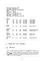
3.4 Specimen input le
This is a small \Attribute and Example" le:
10
**ATTRIBUTE AND EXAMPLE FILE**
% Vertebrate classification
skin_covering: none hair feathers scales;
milk:
yes no;
homeothermic: yes no;
habitat:
land sea air;
reproduction: oviparous viviparous;
breathing:
lungs gills;
class: mammal fish reptile bird amphibian;
@
% mammal
hair
none
hair
hair
yes
yes
yes
yes
yes
yes
yes
yes
land
sea
sea
air
% fish
scales
no
no
% reptile
scales
scales
no
no
% bird
feathers
feathers
% amphibian
none
@
viviparous
viviparous
oviparous
viviparous
lungs
lungs
lungs
lungs
mammal;
mammal;
mammal;
mammal;
sea
oviparous
gills fish w 4;
no
no
land
sea
oviparous
oviparous
lungs reptile w 3.2;
lungs reptile;
no
no
yes
yes
air
land
oviparous
oviparous
lungs bird;
lungs bird;
no
no
land
oviparous
lungs amphibian;
4 Rules: les and evaluation
4.1 File format
When cn2 writes a rule set to le, it does so in a human-readable ASCII form, but
unlike example and attribute les, you are not expected to write or modify rule les
yourself. (i.e. you do so at your own risk, and should note that cn2 does very little
error-checking when reading rule les). In future releases, a graphical interface may
be provided for manipulating rules.
11
A small rule-set appears as part of the trace on page 22.
4.2 Class distributions
The list of numbers at the end of each rule indicates the number of training examples
covered by that rule, divided into classes.
The precise signicance of the counts depends on whether the rules are ordered or
unordered. Ordered rules are intended to be executed in order (!), so the counts
associated with rule refer to the examples covered1 by rule which were
covered by any of the rules 1 through ; 1. This applies also to the default rule|
since this rule has no conditions, its counts comprise all the examples which were not
covered by the preceding rules.
N
N
not
N
The counts associated with each of a set of unordered rules, however, comprise all the
examples covered by that rule including those which may be covered by other rules as
well. Again, this applies equally to the default rule, whose count therefore comprises
the whole example set.
4.2.1 Rare classes
Given the above denition of \class distribution", you might expect that the class
predicted by a rule would always show the largest class-count in the corresponding
distribution; so to avoid possible confusion when using the program, you should note
that this won't always be the case.
In the case of ordered rules, the class predicted by each rule will be the majority class
among the examples covered, by denition.
In the case of unordered rules, however, this property will not always hold, though
it usually will. The exceptions are rules which give better than average predictions
of rarely-occurring classes. For example, in a medical domain, where the program
is trying to predict the rarely-occurring phenomenon of diabetes, the following rule
might be induced:
IF
temperature = high
AND uid-intake = high
THEN diagnosis = diabetes [420 0 0 126]
1
A rule is said to cover an example if the example satises the conditions of the rule
12
where there are 126 examples of diabetes, and 420 of something dierent (colds, as
it happens). Since the occurrence of diabetes in the general population is only 0.1%,
a rule that predicts it with an accuracy of 30% is clearly of some use, even if 70% of
patients satisfying the conditions just have colds.
4.3 Evaluation
The evaluation module takes a set of rules and a pre-classied set of examples, and
compares the classication given by the rules with the given class-values. There are
currently two modes of evaluation: all and individual. (Individual rule evaluation is
a recent addition in response to local demand).
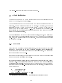
4.3.1 \All" rule evaluation
In this mode, the evaluation is of a set of rules taken as a whole. The results are
displayed in the form of a matrix:
PREDICTED
ACTUAL mammal sh reptil bird amphib Accuracy
mammal
3 0
0
0
0
100 %
sh
0 1
0
0
0
100 %
0 0
1
0
0
100 %
reptile
bird
1 0
1
2
0
50 %
amphibia
0 0
0
0
1
100 %
Overall accuracy: 80 %
Default accuracy: 40 %
The entry in row , column of the matrix is the number of examples classied by
the rules as class which were really of class . (So, in the sample matrix above,
there was 1 example which the rules classied as a mammal, but which was really
a bird.) Fractional values may arise if the examples include \Unknown" or \Don't
Care" values.
i
j
j
i
The \Default accuracy" is only applicable to unordered rule sets; it is the accuracy
resulting from classifying all examples according to the majority class (which is what
the default rule does).
13
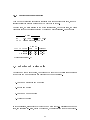
4.3.2 \Individual" rule evaluation
This mode of evaluation is currently available only for unordered rule sets, though a
similar facility for ordered rule sets may be provided in future.
For each rule, a matrix similar to the above is calculated, but in this case, the class
values are reduced to \class predicted by rule" and \other classes". For example:
||||| Rule 2 |||||
IF
7.50 number of legs 25.00
THEN class = spider [0.25 2 0 0]
<
<
FIRED?
ACTUAL CLASS Yes No Accuracy
spider 2.00 0.00 100.0 %
Not spider 0.25 7.75 96.9 %
Overall accuracy: 97.5 %
4.4 Inducing and testing rules
To create and test a set of rules, you will need to carry out the following operations
(the actual commands required are described in the next section).
1. Load some attributes and examples
2. Induce some rules
3. Load some more examples
4. Evaluate the rules
In future releases, I shall probably provide commands for (e.g.) partitioning example
sets, and selecting sub-sets, within the program, thus simplifying the above sequence.
14
5 Using CN
5.1 Interactive use
Note: in specimens of terminal interaction user input appears underlined, and \."
represents the use of the `Return' key. For example:
READ> Both, Atts, or Examples?
READ> Filename? Data/animals
.
Both
In the rst line, the user typed the single character `B' (and did not hit the return
key), and the program expanded the command to `Both'. In the second line, the user
typed the le name `Data/animals', and then hit `Return'.
When you start cn2, you will see this friendly greeting:
********************************
*
*
*
Welcome to CN2!
*
*
*
********************************
followed by the prompt:
CN>
This is the top-level prompt. If you now type `h' or `?' (for help), the program will
display a list of the commands that may be entered at this point, and then re-display
the top-level prompt, ready for another command.
Some operations require several commands to perform. For example, if you want cn2
to read in a le, you have to tell it what sort of thing the le contains, and the name
of the le. In this case, your initial `read' command will cause cn2 to change from
top-level mode to le-reading mode, and it will display a dierent prompt, thus:
READ>
When the le-reading has been completed, cn2 redisplays its top-level prompt, so
the whole sequence might appear as follows:
15
CN> Read
READ> Both, Atts, or Examples? Both
READ> Filename? Data/animals
Reading attributes and examples : : :
10 examples!
Finished reading attribute and example file!
CN>
.
5.1.1 Top-level commands
Note that this section assumes an understanding of the cn2 algorithm as specied in
[Clark, 1989], and you should refer to this document if you are unsure of the meaning
of \star size", \signicance threshold", \ordered rules", etc.
Each of these commands is invoked by typing its initial letter (upper or lower case),
except for \Execute", which is invoked by \x".
Read: Read an attribute, example, attribute-and-example or rule le. When loading
several les in succession, you should bear in mind that cn2 can only retain
in memory one set of attributes, and one set of examples, at any one time.
Consequently:
1. Before loading an example or rule le, you must load the appropriate
attributes.
2. Loading a le of any type overwrites any data of that type which you may
have loaded previously (even if the load fails|for example, because of a
syntax error in the new le).
3. In addition, loading a set of attributes causes any previously-loaded examples to be lost.
The entry of le-names is facilitated by the following features:
1. As in emacs, \ tab " invokes le-name completion. If the prex you
have typed is ambiguous, the program will show you a list of the possible
completions.
2. As in emacs, \ esc h" is bound to \delete-word-backwards".
3. Each time you type a `/' as part of a UNIX path-name, the program checks
that the directory referred to exists and is readable. If not, it will prevent
you from typing further (you must delete back and correct the invalid
path).
<
<
>
>
16
Induce: Run cn2 on the most recently read set of examples. The behaviour of cn2
can be modied by changing various parameters (see the commands below).
However, all these parameters have default values set at start-up, so there is no
need to set them before processing data.
Write: Write a set of rules to le. (You must rst have read in some examples and
run cn2 on them). File-name entry works as for Read, above.
Ckrl: Write data in CKRL format. Either the current set of attributes and examples
(together) or the current decision-tree may be written. Note that the former
option allows cn2 to be used as a translator from cn2 format to CKRL.
eXecute: Enter \evaluation" mode, in which the performance of the current rules
may be assessed with respect to the current examples. (See x 4.3). In evaluation
mode, valid commands are:
All: Evaluate the set as a whole.
Individual: Evaluate rules individually.
Help/?: Display a menu of commands.
RET : Return to the CN prompt.
<
>
>
Algorithm: Specify whether cn2 is to produce ordered or unordered sets of rules.
Error estimate: Specify whether cn2 is to use the Laplacian or the nave estimate
to assess the accuracy of a rule.
The formulae for the two estimates are as follows:
Laplacian: #Correct+1 / #Examples + #Classes
Nave:
#Correct / #Examples
Preciesly which example sets these formulae are applied to depends on whether
the rule set being induced is ordered or unordered (see the discussion of \counts"
in x 4.2).
Star size: Query or alter the star size.
Threshold: Query or alter the signicance threshold.
Display: Provide further information about the search. By default, the program
just displays each rule as it nds it, but if required it can, for example, indicate whenever a new \best node" is found, or which node is currently being
specialised. (Type `h' at the \SET TRACE FLAGS " prompt for a list of
options.)
This facility can be used to clarify what the algorithm is doing, particularly if
it is generating unexpected answers.
>
17
Help/?: Display a menu of commands.
Quit: Quit
5.2 Non-interactive use
It is possible to run cn2 non-interactively by supplying it with a sequence of commands in a le. In this case, cn2 will write a trace of its activities to the standard
output, so if you want to run it in the background, you should redirect its output
either to a log le or to /dev/null. For example:
% cn
<
cn.commands
>
cn.log &
Commands should be listed in the command le more or less as they would be typed
in answer to cn2's prompt. In the case of single-character commands, the complete
command may be used, to make the le more readable (the program will ignore all
but the rst character of the word): each such command should be separated from
the next item by some form of whitespace, but not necessarily a newline. Filenames
must be followed by a newline.
Characters from `#' to the next end-of-line will be regarded as comments and ignored
(c.f. shell scripts).
For example:
read atts Data/animals.atts
read exs Data/animals.exs
alg unordered
star 7
display none quit
induce
write
Data/animals.rules
quit
References
[Boswell, 1990] R.A. Boswell. Manual for NewID version 2.0. Technical Report
TI/P2154/RAB/4/, Turing Institute, January 1990.
[Clark, 1989] P.E. Clark. Functional specication of CN and AQ. Technical Report
TI/P2154/PC/4/1, Turing Institute, September 1989.
18
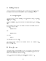
A Getting Started
To read the contents of your release tape, load the tape into your tape-drive, cd to
the directory where you want the sources and data to be installed, and type:
tar xvf tape-device-name
This should create a directory Release, with sub-directories NewId, CN2, Simple Data, and Docs.
Next, cd to Release/CN2, where you should nd the sources for cn2, and a Makele.
If you are using SunOS 3, then you will need to change the denition of \OS" in
\mdep.h". Replace the line:
#define OS (4)
with
#define OS (3)
Now type:
make cn
This will cause cn to be compiled.
You will nd some example and attribute les in the directory Release/Simple Data.
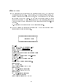
B Example run
This section records a terminal session in which cn2 is applied to a small example
le called `animals'. This le has been included on your release tape, so that you can
experiment with it without having to type it in.
As in x 5.1, user input is underlined, and carriage-return denoted by ..
19
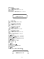
Points to Note
You will notice that in response to the rst `Induce' command, cn2 prints out
the resulting rule set twice. This is because, at the default level of tracing, the
program prints out each rule as it nds it, and then prints out the complete
set of rules when it has nished. In the case of unordered rules, the rules
are not accompanied by class distributions when rst calculated, since it is
more convenient to delay calculation of these distributions until the rule-set is
complete.
x 4.2 discusses the precise meaning of the class distributions.
Note how raising the signicance threshold from 1 to 10 for the second \run"
gives smaller but less accurate rules.
********************************
*
*
*
Welcome to CN2!
*
*
*
********************************
CN> Read
READ> Both, Atts, or Examples? Both
READ> Filename? Data/animals
Reading attributes and examples : : :
10 examples!
Finished reading attribute and example file!
CN> Algorithm
Algorithm is currently set to UN ORDERED
ALGORITHM> Ordered
CN will produce an ordered rule set
CN> Induce
Running CN on current example set: : :
.
Best rule is:
IF
milk = yes
THEN class = mammal [4 0 0 0 0]
Best rule is:
IF
skin covering = feathers
THEN class = bird [0 0 0 2 0]
Best rule is:
IF
skin covering = scales
AND breathing = lungs
THEN class = reptile [0 0 2 0 0]
20
Best rule is:
IF
skin covering = none
THEN class = amphibian [0 0 0 0 1]
Best rule is:
ELSE (DEFAULT) class = fish [0 1 0 0 0 0]
*--------------------------------*
j
j
ORDERED RULE LIST
j
j
*--------------------------------*
IF
milk = yes
THEN class = mammal [4 0 0 0 0]
ELSE
IF
skin covering = feathers
THEN class = bird [0 0 0 2 0]
ELSE
IF
skin covering = scales
AND breathing = lungs
THEN class = reptile [0 0 2 0 0]
ELSE
IF
skin covering = none
THEN class = amphibian [0 0 0 0 1]
ELSE
(DEFAULT) class = fish [0 1 0 0 0]
CN> Algorithm
Algorithm is currently set to ORDERED
ALGORITHM> Unordered
CN will produce an unordered rule set
CN> Threshold
Current threshold is 1.00
New threshold: 7
OK!
CN> Display
SET TRACE FLAGS> None
All tracing is now turned OFF
SET TRACE FLAGS>
CN> Induce
Running CN on current example set: : :
.
.
*-----------------------------------*
j
j
UN-ORDERED RULE LIST
21
j
j
*-----------------------------------*
IF
THEN
milk = yes
class = mammal [4 0 0 0 0]
IF
THEN
skin covering = scales
class = fish [0 1 2 0 0]
IF
THEN
skin covering = scales
class = reptile [0 1 2 0 0]
IF
homeothermic = no
AND breathing = lungs
THEN class = amphibian [0 0 2 0 1]
ELSE (DEFAULT) class = mammal [4 1 2 2 1]
CN> Quit
Have a nice day!
C Handling of Unknowns and Don't Cares
C.1 Training (Learning) Phase
During rule generation, a similar policy of handling unknowns and don't cares is
followed: unknowns are split into fractional examples and dontcares are duplicated.
Strictly speaking, the counts attached to rules when writing the ruleset should be
those encountered during rule generation. However, for unordered rules, the counts
to attach are generated after rule generation in a second pass, following the execution
policy of splitting an example with unknown attribute value into equal fractions for
each value rather than the Laplace-estimated fractions used during rule generation.
C.2 Testing (Execution) Phase
When normally executing unordered CN rules without unknowns, for each rule which
res the class distribution (ie. distribution of training examples among classes) attached to the rule is collected. These are then summed. Thus a training example
22
satisfying two rules with attached class distributions [8,2] and [0,1] thus has an expected distribution [8,3] which results in C1 being predicted, or C1:C2 = 8/11:3/11
if probabilistic classication is desired. The built-in rule executer follows the rst
strategy (the example is classed simply C1).
With unordered CN rules, an attribute test whose value is unknown in the training
example causes the example to be `split'. If the attribute has three values, 1/3 of
the example is deemed to have passed the test and thus the nal class distribution
is weighted by 1/3 when collected. A similar rule later will again cause 1/3 of the
example to pass the test. A don't care value is always deemed to have passed the
attribute test in full (ie. weight 1). The normalisation of the class counts means that
an example with a dontcare can only count as a single example during testing, unlike
NewID where it may count as representing several examples.
With ordered CN rules a similar policy is followed, except after a rule has red
absorbing, say, 1/3 of the testing example, only the remaining 2/3s are send down
the remainder of the rule list. The rst rule will cause 1/3 class distribution to be
collected, but a second similar rule will cause 2/3 1/3 class distribution to be
collected. Thus the `fraction' of the example gets less and less as it progresses down
the rule list. A don't care value always passes the attribute test in full, and thus no
fractional example remains to propagatete further down the rule list.
23