Download Usfos User`s Manual, Solution Strategy

4-1
USFOS USER’S MANUAL
Solution Strategy
4 SOLUTION STRATEGY
The USFOS nonlinear analysis follows the following basic procedure:
•
•
•
•
•
•
4.1
The load is applied in steps
The nodal coordinates are updated after each load step
The structure stiffness is assembled at each load step. The element stiffnesses are then
calculated from the updated geometry.
At every load step each element is checked to see whether the forces exceed the plastic
capacity of the cross section. If such an event occurs, the load step is scaled to make the
forces comply "exactly" with the yield condition.
A plastic hinge is inserted when the element forces have reached the yield surface. The
hinge is removed if the element later is unloaded and becomes elastic.
The load step is reversed (the load is reduced) if global instability is detected.
LOAD SPECIFICATION
USFOS allows for a combined, incremental loading, described by a series of different, subsequent
load vectors.
Each load vector is formed by:
•
•
One basic load case or a combination of up to three basic load cases.
A scaling factor λ, that defines the relative size of the initial (unscaled) load increment.
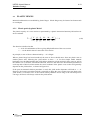
The total series of load vectors then forms the load history of the analysis. This is illustrated by Figure
4.1
2005-07-01
USFOS USER’S MANUAL
Solution Strategy
4-2
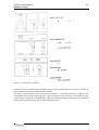
Figure 4.1 Load history definition
Each load vector is repeated a given number of steps, until a specified relative load level is reached, or
until a defined characteristic displacement is attained.
The load is incremented on top of the previous loads, i.e. each load increment is added to the
accumulated load of all previous load steps. The load applied in one load step is continuously acting
on the structure during all succeeding steps. Thus, the calculated results at each step are the combined
results of the total load history prior to and including that step.
2005-07-01
USFOS USER’S MANUAL
Solution Strategy
4-3
Figure 4.2 Combined incremental loading
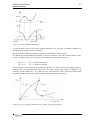
A combined incremental, iterative loading algorithm is implemented. As default, a pure incremental
procedure is adopted. Equilibrium iterations may be specified by the user. At each load step, the
displacements are calculated from the tangential stiffness of the structure. Thus, for the incremental
procedure, the calculated loads will diverge somewhat from the true incremental path as shown Figure
4.3. To ensure satisfactory accuracy, it is recommended to specify small load increments. Generally, a
suitable initial load increment is in the range of 0.10-0.30 of the load at first yield, and should be
reduced when the structural behavior becomes nonlinear, e.g. above the design load.
Figure 4.3 Pure incremental solution technique
2005-07-01
4-4
USFOS USER’S MANUAL
Solution Strategy
The results of different load cases may not be superposed, since the response of the structure is highly
history dependent. Instead, USFOS allows for a combination of the load cases themselves:
One to three basic load cases may be superposed to form a load combination. The various load types
are defined in Section 3.7. This load combination may then be used in the specification of the load
vectors. If no load combinations are defined, the load vector specification is referred to the basic load
case numbers.
Note that if any load combinations are defined, then all load specifications are referred to load
combination numbers. In this case the basic load case cannot be referenced directly, but has to be
defined as a load combination containing only that basic load case.
LOAD INCREMENTATION ALGORITHM
4.2
The automatic load incrementation algorithm consists of two major components
•
•
the sign of the load increment factor ∆p
the size of the load increment factor ∆p (scaling)
4.2.1
Sign of Load Increment
The sign of the load increment is governed by the Current Stiffness Parameter and by the tangential
stiffness matrix determinant.
For load step no. i the Current Stiffness is defined by
∆ r1 ∆ R1 ⎡ ∆ pi ⎤
=
S
⎢
⎥
∆ r iT ∆ R i ⎣ ∆ p1 ⎦
T
i
p
2
(4.1)
where ∆r and ∆R are incremental displacements and forces. ∆p is the relative load increment size at
each load step.
The Current Stiffness Parameter is a normalized parameter representing the stiffness of the structure
during the deformation. It may be regarded as the work carried out in the first load step, divided by
the incremental work at load step no. i. Thus, the current stiffness parameter will have an initial value
of 1.0. For stiffening systems (membrane effects) it will increase. For softening systems, it will
decrease.
2005-07-01
USFOS USER’S MANUAL
Solution Strategy
4-5
Figure 4.4 Current Stiffness Parameter
A small absolute value of the current stiffness parameter will represent an unstable structure, the
instability point having 0.0 Current Stiffness.
During unloading in the post collapse range the Current Stiffness will be negative.
In USFOS, the Current Stiffness Parameter is used to control the sign of the load increment, with a
positive increment as long as Sp is positive, and a negative increment for negative Sp.
∆pi ≥ 0 if
∆pi < 0 if
Spi > 0, positive increment
Spi < 0, negative increment
This procedure is well suited for most problems. However, it fails in case of spring-back problems,
illustrated for a 1-DOF problem in Figure 4.5. The elastic spring-back problem is defined by an
extremely "brittle" behaviour. At a specific level, the load drops with a temporary displacement
reduction until the structure later regains stiffness and the deformation increases.
Figure 4.5 Current stiffness parameter in the elastic spring-back problem
2005-07-01
4-6
USFOS USER’S MANUAL
Solution Strategy
Along path b-c the load should be reduced even if the Current Stiffness is positive. The spring-back
behaviour is often characterized by a large Current Stiffness, Sp > 1 in combination with negative pivot
elements (Gauss reduction terms) in the tangential stiffness matrix. Thus the load increment should
also be reversed when the determinant becomes negative.
In the previous version of USFOS, this situation was controlled by the cmax parameter. Elastic
springback was introduced when the current stiffness parameter exceeded 1.2. The load increment was
then reversed and the load was reduced. With the new load control algorithm the cmax parameter
should no longer be needed and the default value is set to 999. In future program versions this
parameter will probably go out of use.
If the cmax is activated, care should be exercised. When membrane effects dominate a structure's
behaviour, the Current Stiffness Parameter may increase beyond 1.2. In these cases elastic springback should not be introduced, and the user should take care to specify a high value for cmax. An
example of this is the beam with transverse loading shown in Figure 4.6.
Figure 4.6 Elasto-plastic beam bending with membrane effects
The stiffness matrix determinant is the final check used to determine the sign of the load increment.
As long as the determinant is positive (no negative pivot elements), the stiffness matrix is positive
definite, and the structure is 'stable'. As the load increases and the structural response becomes more
and more nonlinear, the determinant will decrease (for softening systems). Zero determinant signifies
a global instability point, and a negative determinant (one or more negative pivot elements) represent
an unstable structure, and the external loading should be reduced. Thus,
∆pi ≥ 0 if
∆pi < 0 if
The tangential stiffness matrix has no negative pivot elements
The tangential stiffness matrix has one or more negative pivot elements
The determinant criterion is controlled by the parameter idetsw.
This leads to the following load control algorithm implemented in USFOS:
Positive increment, ∆pi ≥ 0
if
and
Spi > 0.0
The tangential stiffness matrix has no negative pivot
elements
Negative increment, ∆pi < 0
if
or
or
Spi < 0.0
Spi ≥ Cmax
The tangential stiffness matrix has one or more
negative pivot elements
2005-07-01
USFOS USER’S MANUAL
Solution Strategy
4.2.2
4-7
Size of Increment
The size of the load increment is determined by:
-
The user's load history specification
Introduction of plastic hinges
Exceedance of the user defined maximum displacement increment
The 'arc length' incrementation procedure
Adjustments during equilibrium iterations
The load increment will be scaled down if the element forces at some element end or midspan exceeds
the plastic interaction surface. This check implies that the stress resultants are scaled so as to comply
"exactly" with the yield surface as illustrated in Figure 4.7.
Figure 4.7 Increment scaling due to introduction of plastic hinges
By this procedure only one hinge is detected per load increment. To avoid unreasonably small step
length in case of frequent occurrence of hinges, the Minimum Load Step factor minstp, is specified. In
this way, "exact" scaling to the yield surface is not always possible and several hinges may be inserted
during one load increment.
In regions of unstable equilibrium, some elements may experience a dramatic redistribution of forces
even if the load step is scaled down to the minimum value. The elastic spring-back problem is an
example of this. This may in some cases lead to extreme violation of the yield surface. In order to
avoid this, the Minimum Load Step may be reduced temporarily to 0.01 of the value set by the user.
This is put into effect if the Γ-factor (value of the interaction function) exceeds the value which the
user has specified for the Γ overstepping factor, gamstp. This is illustrated in Figure 4.8.
2005-07-01
4-8
USFOS USER’S MANUAL
Solution Strategy
Figure 4.8 Load increment scaling beyond minstp
In regions where the current stiffness parameter is small, very large incremental displacements may
occur. This may reduce the accuracy of the analysis, as shown in Figure 4.10. Two features have been
implemented to avoid this.
In the arc length incrementation procedure, the size of each increment is compared with the size of the
initial load step of the current load combination. The arc length is defined by
∆ 1i = (| ∆ R i | )2 + (| ∆ r i | )2
(4.2)
or normalized:
2
⎛|∆ i |⎞ ⎛ |∆ i |⎞
∆ 1 = ⎜⎜ R0 ⎟⎟ + ⎜⎜ r0 ⎟⎟
⎝ | ∆ R |⎠ ⎝ | ∆ r |⎠
2
i
(4.3)
Thus, each load increment is scaled such that
∆ 1i ≤ ∆ 10
(4.4)
This is illustrated in Figure 4.9.
The normalized arc length of the initial step will be ∆p0 = √2. Thus, the load increment can increase to
1.4 times the initial load increment for very high stiffness, (∆ri=0), whereas displacement increment
can be increased up to 1.4 times the initial displacement increment for very small stiffnesses, (∆Ri=0).
However, since the initial (elastic) displacement can be quite small, a maximum displacement
increment of 1.4 times this size may give far too small steps throughout the analysis. To compensate
for this, the 'mxpdis' parameter ("max displacement increment") has been included in the expression.
Thus, the arc length is governed by an elliptic expression, rather than a circle:
2
2
⎛|∆ i |⎞ ⎛ |∆ |
1 ⎞
∆ 1 = ⎜⎜ R ⎟⎟ + ⎜⎜ r0i •
⎟⎟ ≤ ∆ 10
|
|
|
|
mxpdis
∆
∆
⎝ R0 ⎠ ⎝ r
⎠
(4.5)
i
2005-07-01
4-9
USFOS USER’S MANUAL
Solution Strategy
Ρ ΕΞΤ
∆Ρ
∆Ρ
∆λ
ι
∆ ρι
0
∆λ
0
∆ρ
ι
ρ
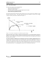
Figure 4.9 Arc length increment scaling
In addition to the arc length scaling (based on the norm of all degrees of freedom), the user may
specify a number of characteristic control displacements for the structure. The weighted sum of these
displacements form a "global" displacement for the structure, calculated by:
∑ ∆ r ik ⋅ ω k
, k = 1, NCNOS
∑ωk
ω k = weight factor associated with control displacement k
i
∆ r k = displacement increment for control displacement k at step i
∆ r iglob =
(4.6)
The load step will be scaled down if the control displacement increment of the current step exceeds the
mxpdis times the control displacement of the initial load step of that load combination.
∆ r iglob ≤ mxpdis ⋅ ∆ r iglob
(4.7)
2005-07-01
USFOS USER’S MANUAL
Solution Strategy
4-10
Figure 4.10 Scaling by maximum control displacement increment
If only one degree of freedom is specified, the control displacement will not be normalized. I.e. the
control DOF will only be multiplied by the weight factor.
4.2.3
Equilibrium Iterations
The Euler-Cauchy incrementation algorithm generally causes a drift-off from the exact solution path.
Corrections for this deviation can be taken care of by specifying equilibrium iterations on the
unbalance between external loads and internal forces after each load step. The approach used is the
pure Newton- Raphson method with arc length control.
In the pure Newton-Raphson method the tangent stiffness matrix is updated after each iteration level.
New plastic hinges are inserted if so should be necessary. Elastic unloading in yield hinges is not
allowed, because the unbalanced load vector may be alternating and therefore cause an unstable
behaviour.
A common problem associated with equilibrium iterations, is that the iteration procedure fails
(diverges) when passing load limit points or bifurcation points. To overcome these problems, an arc
length iteration procedure has been implemented in USFOS, with a special algorithm for passing load
limit points or bifurcation points.
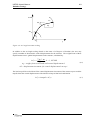
The arc length iteration procedure is implemented with iterations to a normal plane. That is, instead of
keeping the external load level fixed during iterations, the external load and displacement vectors vary
according to a prescribed function in the 'load-displacement space'. In the current formulation, the
loads and displacements are forced to move along a plane normal to the direction of the original load
and displacement increment. This is illustrated in Figure 4.11.
2005-07-01
4-11
USFOS USER’S MANUAL
Solution Strategy
Ρ ΕΞΤ
∆π ϕ
∆ Ρ ι,0
ι
∆ ρι,0
ρ
∆ ρι,1
Figure 4.11 Arc length iterations
Iterations have converged when the change in load and displacement becomes smaller than a specified
limit. This is expressed by the following parameters :
δ r itj =
| ∆ r i, j |
| ∆ r i,0 |
| ∆ i, j |
δ R = Ri,0
|∆R |
(4.8)
i
it
where ∆Rij and ∆rij are the load and displacement vectors at iteration j of step i, and ∆Ri0 and ∆ri0 are
the load and displacement increments for step number i. Both parameters are initially equal to unity,
and approach zero when the iterations converges. They are listed in the analysis print file, but only δrit
is used for the convergence test. The actual convergence criterion is defined by the parameter epsit.
exceeded.
δ rit ≤ ε it
(4.9)
In addition, iterations are controlled by an algorithm to detect load limit points/bifurcation points as
follows :
The Current Stiffness and the stiffness matrix determinant are calculated at each iteration. A load
limit point or bifurcation point is identified by the load control algorithm in Section 4.2, that is, if
either the Current Stiffness or the stiffness matrix determinant changes sign from iteration j-1 to
iteration j. If a limit point or a bifurcation point is detected, the iterations at the current load step are
terminated. The results from the last iteration (j-1) are accepted as the results of the load step even if
equilibrium has not been obtained.
2005-07-01
4-12
USFOS USER’S MANUAL
Solution Strategy
At each load step in the analysis, the possible loading direction can be described by the following 5
sectors,
Figure 4.12:
1.
2.
3.
4.
5.
Stable loading (Cmax > Sp ≥ Cmin)
This sector describes stable loading conditions, with Current Stiffness, Sp below the spring-back
limit, Cmax and above the 'zero stiffness'limit, Cmin. Default Cmax=999.
'Zero stiffness' (Cmin > Sp ≥ Cminneg)
The user can suppress iterations in regions of small structural stiffness. A positive and a negative
value for a 'minimum iteration stiffness' is specified. Default values for both Cmin and Cminneg are
0.000.
Stable unloading (Cminneg > Sp ≥ Cneg)
This sector describes stable unloading conditions, with Current Stiffness below the negative
'Zero stiffness' limit, Cminneg, but above the limit for 'unstable unloading', Cneg.
Unstable unloading (Cneg > Sp)
This sector describes unstable unloading conditions, defined by the parameter Cneg.
'Spring-back' behaviour (Sp > Cmax)
This sector contains extreme unloading conditions, 'Spring back behaviour'.
Χµαξ
1
3
5
4
Χ±∞
Χ µιν
Χµιν νεγ
Χνεγ
Figure 4.12 Loading regimes
In general, iterations are performed as long as the Current Stiffness parameter stays in the same sector
during the load step. If Sp changes sector, this is an indication of a load limit point, and iterations are
terminated.
2005-07-01
USFOS USER’S MANUAL
Solution Strategy
4.3
4-13
PLASTIC HINGES
Material nonlinearities are modelled by plastic hinges. Plastic hinges may be inserted at element ends
or at midspan.
4.3.1
Elastic-perfectly-plastic Model
The plastic capacity of a cross-section is represented by a plastic interaction function/yield surface for
stress resultants
⎛ N Q y Qz M x M y M z ⎞
⎟ - 1= 0
Γ= f ⎜
,
,
,
,
,
⎜ N p Q Q M xp M yp M zp ⎟
yp
zp
⎠
⎝
(4.10)
The function is defined so that
Γ = 0 for all combinations of forces giving full plastification of the cross section
Γ = -1 is the initial value of a stress-free cross section
In principle, a state of forces characterized by Γ > 0 is illegal.
When a plastic hinge has been introduced, the state of forces should move from one plastic state to
another plastic state, following the yield surface so that Γ = 0. For this simple model material
hardening is not included and thus the yield surface maintains a fixed position in force space as well as
the surface size is constant. It should be observed, however, that due to the linearization performed at
each step and to finite load increments the stress resultants of the plastic cross-section will generally
depart from the yield surface , as shown in Figure 4.13.
If the pure incremental solution procedure is used, this yield surface departure will lead to Γ > 0.
However, the iterative procedure include a correction to bring the cross section force state back to the
yield surface, see Section 4.4.1 of the USFOS Theory Manual. And as long as the iteration process
converge, the forces will always reside on the yield surface.
2005-07-01
USFOS USER’S MANUAL
Solution Strategy
4-14
Figure 4.13 Cross-sectional yield surface
4.3.2
Partial Yielding and Strain Hardening Models
The material model which accounts for partial plastification and strain hardening is formulated
according to the bounding surface concept /1/.
This model employs two interaction surfaces as shown in Figure 4.14, namely the yield surface and
the bounding surface. Both surfaces are derived from conventional cross section interaction curves for
the cross section considered, and are defined in the normalized force space as indicated in Figure 4.14.
The yield surface bounds the region of elastic cross sectional behaviour and when the force state
contacts the yield surface this corresponds to initial yielding in the cross section. This condition is
written as:
F y = f y (n, q y , q z , m x , m y , m z , z y ) - 1 = 0
(4.11)
where
n=
Qy - β 2
N - β1
Q - β3
M y - β5
M z - β6
M x - β4
, mz =
,qy = z
,mx =
,my =
,qy =
Q py ⋅ z y
N p ⋅ zy
M yp ⋅ z y
M zp ⋅ z y
A pz ⋅ z y
M xp ⋅ z y
(4.12)
and 0 < zy < 1 denotes the yield surface extension parameter. βi, i = 1,6 is the translation of the yield
surface in force space from the initial position corresponding to a stress-free cross section.
2005-07-01
USFOS USER’S MANUAL
Solution Strategy
4-15
The bounding surface determines the state of full plastification of the cross section. This surface,
which has the same shape as the yield surface, is defined by the function:
F b = f b (n, q y , q z , m x , m y , m z , z b ) - 1 = 0
(4.13)
where the arguments of fb are given by Eg. 4.3.3 when substituting βi and zy by αi and zb, respectively.
αi is the bounding surface translation and zb the bounding surface extension parameter which is equal
to unity.
Figure 4.14 illustrates the yield and bounding surface for a tubular cross section plotted in the mz, n plane. Here zb = 1.0 and zy = 0.79 corresponding to the ratio of the elastic to the plastic cross sectional
modulus in bending. When loading the cross section the force point travels through the elastic region
and contacts the yield surface indicating initial yielding in the cross section, see Figure 4.14a. At this
stage a plastic hinge is introduced.
When further loading takes place the yield surface is forced to translate such that the force state
remains on the yield surface (Fy = 0), see Figure 4.14b. At this stage the bounding surface also
translates, but at a much smaller rate.
The translation of the yield surface, which approaches the bounding surface during the loading
process, provides for a smooth transition from initial yield to full plastification.
In Figure 4.14c the force state has reached the bounding surface which corresponds to full
plastification of the cross section. From this stage the force state is forced to remain on the bounding
surface and additionally both surfaces will translate in contact.
The translation of the bounding surface is in fact used to model strain hardening, i.e. a kinematic
hardening model is used.
A parameter ai, defined for each force component, determines the form of the transition phase from
initial yield to full plastification and should be selected on basis of experiments. For increasing ai the
transition region, for instance for the M - θ relationship, decreases.
A parameter ci, defined for each force component, determines the rate of strain hardening. This
corresponds to the translation rate of the bounding surface in force space. Increasing ci increases the
material hardening.
2005-07-01
USFOS USER’S MANUAL
Solution Strategy
Figure 4.14
4-16
Partial yielding and strain hardening formulated according to the
bounding surface concept
2005-07-01
USFOS USER’S MANUAL
Solution Strategy
4.4
4-17
ELASTIC UNLOADING/ELEMENT STATUS
At each step the plastic displacement increment, ∆λ, is calculated for each plastic hinge. If ∆λ is
positive, the hinge remains in a state of plastic loading. If ∆λ is negative, elastic unloading takes
place. The assumption of a plastic hinge at the actual cross-section is then no longer valid, and the
entire load step is recalculated.
The incremental stiffness matrices for those elements which experienced unloading at some location
are then modified, and the load step is repeated. Other hinges may show elastic unloading during
recalculation, and the process is repeated until all unloading hinges are restored to the elastic state.
After a number of trials the load step is nevertheless accepted, even if unloading plastic hinges remain.
In that case the load increment is scaled down to minimum (minstp). In the present version of USFOS,
the number of trials is set to 5. This number may be changed by the user with the ktrmax parameter .
It should be emphasized that this parameter normally has very little impact on the calculation results,
and should only be changed in very special cases.
The elastic unloading event has also some impact on the control of subsequent plastic hinge formation.
This is illustrated in Figure 4.15. Due to finite load increments the stress resultants depart from the
yield surface. Thus, unloaded hinges may still have Γ > 0. In order to avoid false plastification a
plastic hinge is only inserted if Γi > 0 AND Γi > Γi-1.
Figure 4.15 False plastification
The element status is updated every time a plastic hinge is inserted or removed. The possible beam
element status are shown in Figure 4.16. The element status moves up and down this hierarchy
according to the current number of hinges.
However, it is not possible to transfer from ES ≥ 4 to ES < 4. When a plastic hinge is introduced at
element mid-span, the element is divided into two new sub-elements. Due to permanent plastic
displacement at the mid hinge, the beam must still be divided into two sub-elements, even if the mid
hinge has unloaded. This is flagged by a negative element status value (ES = -4, -5, -6, -7)
2005-07-01
USFOS USER’S MANUAL
Solution Strategy
4-18
Figure 4.16 Beam element status
The element status and the Γ-values are listed in the print file. The accuracy of the stress resultants
with respect to the yield condition (plastic interaction function) can then be checked (Section 8.1.4).
4.5
CONTROL OF PLASTIC HINGES
The maximum number of plastic hinges allowed to develop at a node is equal to the number of beams
connected to the node, minus one. This means that at least one beam end should remain elastic to
prevent ill-conditioning of incremental equations. This implies no approximation, because force
equilibrium at the node is preserved. However, the distribution of plastic displacements among the
member ends may be affected.
Exceptions are made for nodes where all rotational degrees of freedom are fixed. All beam-ends are
then allowed to be plastic.
The maximum number of plastic hinges defined above can be overwritten by a value specified by the
user.
Furthermore, it is possible to suppress introduction of plastic hinges at specified element locations.
The cross-section will then remain elastic and large violations of the yield surface may take place.
4.6
ACCURACY OF EQUATION SOLVER
A solution tolerance parameter, also called condition parameter is defined as:
⎡| smallest pivot |
⎤
TOL = MIN ⎢
;| smallest pivot |⎥
⎣ | largest pivot |
⎦
(4.14)
2005-07-01
USFOS USER’S MANUAL
Solution Strategy
4-19
The parameter gives an indication of the accuracy of the equation solution at a given state of
deformation.
Generally, the condition of the tangential stiffness matrix will decrease gradually during the
incremental loading process.
A high value, e.g. 10-2, indicates that the incremental equations are well-conditioned whereas a low
value, e.g. 10-9, indicates ill-conditioning. A zero condition parameter implies a singular matrix. The
condition parameter will be tested against a minimum admissible value epssol and calculation will be
stopped with a fatal error message if TOL < epssol.
The default value is epssol = 10-20. This value is very low, but it prevents the program from an
unwanted stop close to a global instability. The default value of epssol can be changed by the user .
4.7
BIFURCATION ANALYSIS
The detection of a bifurcation point in the solution path is based on Eq. 5.2 in the USFOS Theory
Manual. The determinant of the tangential stiffness matrix becomes zero while the current stiffness
parameter Sp remains positive.
If bifurcation analysis is specified in the control file, the eigenvalues and corresponding eigenvectors
are written to the print file at the load step at which bifurcation is detected. In addition, the
eigenvectors are written to a user specified file (type bif) as nodal point loads according to the
BNLOAD card format. To each loadvector or eigenvector a load case number is allocated. The
number is equal to the sum of loadcases specified in the input and the eigenvector sequence number.
Depending on the CBIFURC input parameters, the solution may be advanced or terminated at the
bifurcation point for visual inspection of the buckling modes by XFOS. If the latter option is chosen,
the eigenvectors are stored as global result data by USFOS and may subsequently be presented
graphically by XFOS. The buckling modes are identified by the loadcase/combination number at
which bifurcation occur and a load step number, which is increased by the eigenvector sequence
number.
The experience with the bifurcation analysis so far is limited, and the option should be used with care.
For complex structural systems, it may be troublesome to select the "correct" buckling mode to impose
on the structure. It should be noted that if the solution seems to degenerate even more when a buckling
mode is injected, it is an indication that the choice of eigenvector was poor.
In the following a procedure for traversal of bifurcation points is proposed which may be employed if
serious problems are encountered in the automatic solution procedure, see Figure 4.17:
1. Perform an initial analysis with bifurcation point detection switched on from a step prior to the
step where bifurcation occur.
2. Eigenvectors are written to the bifurcation load file. Continue the analysis or stop for buckling
mode inspection and restart.
3. Restart from at step prior to the bifurcation point. Impose a chosen eigenvector as nodal loads at
the bifurcation point or a few steps prior to this. The buckling mode is injected by specifying the
eigenvector load case number in the CUSFOS card.
The sign and magnitude of the injected load vector must also be specified by the user. Modify the
CBIFURC parameters so that bifurcation point detection becomes active once the bifurcation
point is traversed or remove the CBIFURC record completely if no more bifurcation point are
anticipated.
2005-07-01
4-20
USFOS USER’S MANUAL
Solution Strategy
4. Verify that the solution improves at the bifurcation point. If not, select another buckling mode or
accept the solution already found.
5. The procedure 1-5 may be repeated to traverse consecutively detected bifurcation points
R
bifurcation
point
bifurcation
point
r
Bifurcation active
Eigenvalue analysis
Bifurcation active
RESTART
Buckling mode injection
Figure 4.17 Bifurcation point analysis
2005-07-01
4-21
USFOS USER’S MANUAL
Solution Strategy
4.8
GUIDELINES FOR ANALYSIS SPECIFICATION AND VERIFICATION
The aim of this section is to give some simple rules of thumb in the use of USFOS. These points are
mainly based on experience from analyses of offshore jacket structures, but the basic considerations
should be applicable to other areas as well.
As in most nonlinear analyses, the load steps may be large as long as the structure behaves "linearly".
For increasing nonlinearity in the structural behaviour, the load steps should decrease. That is, the
optimum load specification is closely linked to the nonlinear characteristics of the structure itself.
In the USFOS formulation, this problem is partly solved by the automatic load scaling used when
plastic hinges are introduced, but the user still have to supply sensible values for the size of the initial
load increment (load factor λ, Section 4.1) and for the minimum load step in the load scaling
algorithm (Section 4.2).
The correct size for these parameters will be a compromise between accuracy and time/cost, and the
right load specification will often be determined through an iterative process as outlined below:
1.
Determine an initial load history, based on the a priori knowledge of the structural behavior (e.g.
linear elastic analyses).
2.
Check the global behavior of the structure, if significant and sudden redistribution of forces
seems to occur at any load level. Check if the load increments at this load level were small
enough to capture these effects.
3.
Check the interaction function at the plastic hinges whether the Γ-values are acceptable, or if the
state of forces show significant exceedance of the yield surface.
4.
Determine at which load level the analysis accuracy deteriorates.
5.
If analysis results beyond this load level is required, then specify a new load history and restart
the analysis for this load level.
Repeat from step 2.
2005-07-01