Download Path Tracking and Obstacle Avoidance for a Miniature Robot

Path Tracking and Obstacle Avoidance for a Miniature
Robot
By
Martin Lundgren
Master Thesis 2003
Department of Computer Science
Umeå University
Abstract
Path tracking and obstacle avoidance are two very important behaviours that must be
considered in the process of developing Autonomous Ground Vehicles, AGV:S. An AGV is a
vehicle with the ability to operate all by itself at ground level, that is an unmanned vehicle
under the control of a computer. A lot of progress has been done in the field of developing
AGV:s in the last decade, and successful applications has been made in both mining and
agriculture. Now the research is starting to concentrate on developing an AGE that can
operate in forest-like environments. It is in this kind of challenging environments that path
tracking and especially obstacle avoidance becomes very important issues.
When in path tracking mode, the vehicle is travelling along a memorized path under the
complete control of a computer. The path has then been memorized by letting a human
operator manually remote the vehicle along a predefined path. If the AGV during the process
of path tracking detects any new obstacles on the path, the obstacle avoidance routine should
find a new route around the obstacle and then return on the path.
In this project I will implement and evaluate algorithms for path tracking and obstacle
avoidance on a miniature robot. The work is related to similar problems in the IFOR-project
[4]. The robot I will be working with is the Khepera model, a two-wheeled differential steered
small robot that uses eight proximity sensors and a camera module for detection of obstacles.
I will study and evaluate the performance of existing well known path tracking algorithms,
like follow-the-carrot and pure-pursuit, as well as the more recently developed vector-pursuit
tracking method.
As for the obstacle avoidance behaviour, I noticed that a simple local algorithm would be
suitable in this project, because of lacking precision in the Kheperas ability to detect
obstacles. The Matlab environment is used for all implementation and testing, as well as the
displaying of tracking routes and evaluations of the various methods.
Index
1
2
3
4
5
6
7
8
9
Introduction ........................................................................................................................ 6
The Khepera robot.............................................................................................................. 7
2.1
Overview .................................................................................................................... 7
2.2
Sensors ....................................................................................................................... 8
2.3
Connections and communication ............................................................................... 9
Dead Reckoning ............................................................................................................... 10
3.1
Basics ....................................................................................................................... 10
3.2
Differential drive kinematics.................................................................................... 11
3.3
Pros and cons............................................................................................................ 13
Path Tracking ................................................................................................................... 13
4.1
Follow-the-carrot...................................................................................................... 14
4.2
Pure Pursuit .............................................................................................................. 15
4.3
Vector Pursuit........................................................................................................... 17
4.4
The look-ahead distance........................................................................................... 19
Implementation issues ...................................................................................................... 20
5.1
Dead-reckoning unit................................................................................................. 20
5.2
Remote unit .............................................................................................................. 21
5.3
Obstacle Avoidance unit .......................................................................................... 22
5.4
Path Tracking units................................................................................................... 24
Tests And Evaluations...................................................................................................... 25
6.1
Method for evaluating the algorithms ...................................................................... 25
6.2
Results ...................................................................................................................... 26
6.2.1
Survey............................................................................................................... 26
6.2.2
Evaluation......................................................................................................... 28
6.2.3
So why the small differences?.......................................................................... 32
6.2.4
Pure-pursuit vs. Vector-pursuit ........................................................................ 33
6.3
Summary of results and conclusions........................................................................ 35
Appendix A ...................................................................................................................... 36
7.1
Simple Square .......................................................................................................... 36
7.2
S-curve ..................................................................................................................... 38
7.3
8-figure ..................................................................................................................... 40
7.4
Path with a displacement section ............................................................................. 42
Appendix B ...................................................................................................................... 44
References ........................................................................................................................ 50
4
5
1 Introduction
Developing an unmanned vehicle with the ability to autonomously transport timber from the
area of felling to the main roads for further transportation to the factories is not an easy task.
Several important factors must be considered in the planning phase of such a project. Among
the most important ones are of course the safety issues involved – a vehicle that large moving
autonomously in a forest environment has to have very accurate sensors for detection of
humans as well as other obstacles in the vicinity of the vehicle. In addition to this some good
behaviours must be implemented in the on board computer for dealing with situations
involving obstacles of any kind. Another important part of the project is the path tracking
behaviour of the vehicle. This behaviour is made up of two parts. The first part is the
recording phase, for which a human operator manually remotes the vehicle along a
predefined path and a computer is recording all of the route travelled. Naturally the second
phase is the path tracking mode, and in this mode the computer takes full control of the
vehicle, following the recorded route as close as possible considering any biases that could
accumulate position and heading errors along the way. During this second phase any obstacles
detected in the direction of travel would either cause the vehicle to stop and return control to
the driver, or in case of static obstacles like trees or stubs a detour around and then returning
to the original track.
This project is related to the problems above. I will implement, test and evaluate a number of
the existing path tracking algorithms available today, trying to figure out which of these
would be most appropriate to integrate in a forest machine like the one mentioned previously.
Although this tests will only be performed on a miniature robot called Khepera, the results
gained can help ease things for the original IFOR-project.
I have divided the report in two main sections; the first part consists of all the theory related to
the project, and in the second part I present and display the results gained from testing the
methods in different situations, and evaluate them accordingly. In the first section I will
initially describe the robot used for all experiments, then some important theory behind the
localization of the robot in an unknown environment, followed by a brief explanation of the
path tracking algorithms that has been implemented and tested on this robot. The evaluation
part consists of display and analysis of four different types of paths. I have compared the
methods to each other on basis of mean and maximal deviation from the path, depending on
variables like speed and look-ahead distances.
6
2 The Khepera robot
2.1 Overview
Khepera is a miniature robot especially well suited for laboratory experiments in a school
environment [8]. It was originally developed by the LAMI team of the EPF in Lausanne
Switzerland, and it’s commercially available at the K-Team S.A. Kheperas small size, only
5.5 cm in diameter, gives it a lot of advantages in many different areas. One advantage is the
possibility to have the robot on a desk close to the computer when performing experiments
and tests of different algorithms. A miniature robot of this kind further allows easy
manipulation and reduces the effort needed for transportation to other locations. One also has
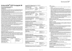
the possibility to increase functions by adding extension turrets on top of the base unit. Below
you can see a picture of this base module.
Fig 1. Khepera base module
The Khepera robot is only equipped with two wheels that does both the steering and
propulsion. This kind of drive mechanism is called differential drive, and is often used on
small miniature robots of this kind. Each of the two wheels is controlled by a DC motor
through a 25:1 reduction gear box. An incremental magnetic encoder is mounted on each
motor and returns 24 pulses per revolution of the motor, which allows a resolution of 600
pulses per revolution of the wheel. This corresponds to 12 pulses per millimetre of path of the
robot or 0,08 millimetre per pulse, considering the wheel diameter. The maximum speed
according to the specifications is 60 cm/s, and the minimum is 2 cm/s.
The standard processor type is a Motorola 68331 with a frequency of 38 MHz and a RAM
consisting of 256 Kb. Its is powered either by an adapter through an S serial line connector or
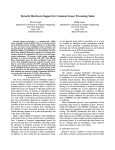
by rechargeable batteries. An overview of the Khepera robot from different angles is shown
below:
7
Fig 2. Overview of some parts on the Khepera robot
Numbered parts:
1.
2.
3.
4.
5.
6.
7.
LEDs
Serial line(s) connector
Reset button
Jumpers for the running mode selection
Infra-Red proximity sensors
ON-OFF battery switch
Second reset button (same function as 3)
2.2 Sensors
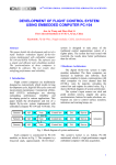
The Khepera is also equipped with eight proximity sensors placed around the base module
according to fig 3. These sensors consist of an integrated IR emitter and receiver which allows
two types of measurements:
•
Ambient light measurement. This measurement is performed using only the receiver.
The emitter is totally inactive. The sampler rate is 20 ms. Activation and reading of a
single sensor takes 2.5 ms to complete.
•
Measurement of light reflected from obstacles. This type of measurement is done by
using both the emitter and the receiver. The difference between the two values is
returned. The sample rate, and the activation and reading time are the same as for the
ambient light measurement.
8
Fig 3. Position and orientation of
sensors on the base module
The values returned from these proximity measurements depends on factors like colour, shape
and intensity of the obstacle detected, as well as the distance to the light source. I noticed that
white objects was preferable - the more darker an object the worse accuracy of measurement.
At optimal conditions the proximity sensors can detect obstacles at a maximum distance of 50
mm, although in my experiments this distance surely wasn’t greater than 30 mm. The values
returned from proximity readings varies from 0 to 1024 - 0 indicating that no obstacle was
detected, a larger value points to the opposite. The high frequency of noise in the readings is a
disadvantage, making the measurements less reliable and the experiments more unstable.
Noise results in readings indicating the false presence of obstacles, and is caused by light
reflections.
2.3 Connections and communication
Only two connections is needed, one is used for recharging of batteries and the other for
connection between robot and computer. Communication between robot and host computer is
done through a RS232 line, which is converted by the interface module to a S serial line
available on the robot. The S serial line connects the robot with the interface module, and is
also responsible for the Kheperas power supply. Another connection is made between
interface module and host computer by the RS232 line, and last but not least the interface
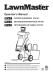
module is connected to the power supply. This yields the communication configuration of the
Khepera, which is also shown in figure 4.
Fig 4. Robot – computer
Communication configuration
9
Robot and host computer communicates by sending and receiving ASCII messages. The host
computer initiates communication by sending a command to the Khepera followed by a
carriage return or a line feed. Then a response is sent by the robot to the host to confirm
message was received and executed. This procedure corresponds to a master – slave protocol,
with the host computer taking on the role as master and the robot gets to be the slave. All
commands consists of a single capital letter, sometimes followed by numerical or literal
parameters separated by a comma and terminated by a linefeed. Responses comes in the form
of the command letter in lower case, followed by potential numerical and literal letters
depending on the command sent.
3 Dead Reckoning
3.1 Basics
Dead reckoning is a method used for determining the current position of a vehicle, by
advancing some previous position through known course and velocity information over a
given time period [1]. Or more simply put, a process of estimating the position of a vehicle
based solely on speed, direction and time elapsed since the last known position. Dead
reckoning was probably derived from the term deduced reckoning by sailors sometimes in the
seventeenth century. Theory has it someone abbreviated this to ded reckoning in the ships log,
and later on another unknown person must have thought it was a misspelling for dead. There
are more theories behind the origin of the term, but this is the most commonly used today.
Most of the robotic ground vehicles today rely on dead reckoning as the framework of their
navigational systems. One simple way to implement dead reckoning is called odometry.
Odometry is a method to provide information about vehicle displacement based on the
rotation of its motors or wheels. The rotation is measured by wheel or shaft encoders. These
encoders counts the number of rotations of the wheel axles, providing data that combined
with the forward kinematics equations can be translated to information regarding the change
in position and heading of the vehicle. Figure 5 shows a picture of the normal configuration
and placement of encoders and motors on a differential drive ground robot vehicle, like the
Khepera.
Fig 5. Differential drive mobile robot
10
What then is forward kinematics? Kinematics is the study of motion, but without having to be
concerned with the forces that affect the motion. The problem of determining what positions
that is reachable given only the velocities of the wheels is called forward kinematics.
3.2 Differential drive kinematics
The theory behind differential drive kinematics is pretty straightforward. Every wheeled
mobile robot in a state of motion must always rotate about a point that lies somewhere on the
common axis of the two wheels [6]. This point is often called the instantaneous centre of
curvature (ICC), or the instantaneous centre of rotation (ICR). A differential drive robot, like
the Khepera, changes the position of the ICC simply by varying the velocities of the two
wheels. Two separate drive motors, one for each wheel, provide independent velocity control
to the left and right wheels. It is this property that makes it possible for the robot to choose
different trajectories and paths. A sketch describing the kinematics of a differential drive
mobile robot can be seen in figure 6.
Fig 6. Differential drive kinematics
Each wheel follow a path that moves around the ICC at the same angular rate ω [6], thus
ω(R + l/2) = vr
ω(R - l/2) = vl
where l is the distance between the two wheels, the right wheel moves with velocity vr and
the left wheel moves with velocity vl. R is the distance from the ICC to the midpoint
between the wheels. All these control parameters are functions of time, which gives
R = l/2 * (vl + vr)/(vr – vl)
ω = (vr – vl)/l
We have two special cases that comes from these equations. If vl = vr, then the radius R is
infinite and the robot moves in a straight line. If vl = -vr, then the radius is zero and the
11
robot rotates in place. In all other cases the robot moves in a trajectory around the ICC at
some angular rate ω.
The forward kinematics equations can be derived easily now that we have established the
basics. Our focus is on how the x and y coordinates and the orientation change with respect to
time [2]. Let θ be the angle of orientation, measured in radians, counter-clockwise from the xaxis. If we let m(t) and θ(t) be functions of time representing speed and orientation for the
robot, then the solution will be in the form:
dx/dt = m(t)cos(θ(t))
dy/dt = m(t)sin(θ(t))
(3.1)
(3.2)
The change of orientation with respect to time is the same as the angular rate ω. Therefore
dθ/dt = ω = (vr – vl)/l
(3.3)
Integrating this equation yields a function for the robots orientation with respect to time.
The robots initial orientation θ(0) is also replaced by θ0:
θ(t) = (vr – vl)t/l + θ0
(3.4)
Since the velocity in functions (3.1) and (3.2) above simply equals the average speed for the
two wheels, that is m(t)=(vr+vl)/2, integrating this in (3.1) and (3.2) gives:
dx/dt = [(vr + vl)/2]cos(θ(t))
dy/dt = [(vr + vl)/2]sin(θ(t))
(3.5)
(3.6)
The final step is to integrate equations (3.5) and (3.6), and taking the initial positions to be
x(0) = x0, and y(0) = y0 to get:
x(t) = x0 + l/2(vr + vl)/(vr - vl)[sin((vr - vl)t/l+ θ0)-sin(θ0)]
y(t) = y0 - l/2(vr + vl)/(vr - vl)[cos((vr - vl)t/l+ θ0)-cos(θ0)]
(3.8)
(3.9)
Noting that l/2(vr + vl)/(vr - vl) = R, the robots turn radius, and that (vr - vl)/l = ω, equations
(3.8) and (3.9) can be reduced to:
x(t) = x0 + R[sin(ωt + θ0)-sin(θ0)]
y(t) = y0 - R[cos(ωt + θ0)-cos(θ0)]
(4.0)
(4.1)
This is the theory that lies behind implementing dead reckoning on a wheeled mobile robot
using differential steering. The only thing one has to do is to substitute the terms vr and vl
with sr and sl, indicating the calculations of displacements rather than speeds, and as a result
of this also drop the time value t. Here sr and sr are the distances traveled by the left and right
wheels respectively. Finally when this has been done equations (3.8) and (3.9) becomes:
x(t) = x0 + l/2(sr + sl)/(sr - sl)[sin((sr - sl)/l+ θ0)-sin(θ0)]
y(t) = y0 - l/2(sr + sl)/(sr - sl)[cos((sr - sl)/l+ θ0)-cos(θ0)]
(4.2)
(4.3)
which are the forward kinematics equations used by differential drive vehicles when turning.
12
3.3 Pros and cons
What is the pros and cons implementing odometry based dead reckoning as the navigational
system on a wheeled mobile robot? Odometry is very inexpensive compared to other
methods, like GPS or ground beacon systems. It doesn’t require complex mathematical
calculations, yet providing rather good short term accuracy. Another advantage is the high
sampling rates, which further enhances the positional accuracy compared to methods with a
slower sampling rate. But with so many other things in the world, there is also a bunch of
disadvantages involved. One primary disadvantage with odometry is its tendency to
accumulate errors over time. There are mainly two types of errors that can be accumulated in
systems based on odometry: systematic errors and non-systematic errors. Systematic errors
are caused by flaws in the mechanical design of the robot, that is internal model-specific
errors most often created by unequal wheel diameters or uncertainty about what wheelbase is
the most effective. Non-systematic errors on the other hand are caused by external factors and
not by the kinematics properties of the vehicle. Wheel-slippage and rough floor surfaces
containing irregularities are examples of this kind of errors. Systematic errors are worse than
environment depended errors, because they accumulate constantly. Despite these drawbacks
many researchers are convinced that dead reckoning still is an important part of robot
navigation.
4 Path Tracking
Path tracking is the process concerned with how to determine speed and steering settings at
each instant of time in order for the robot to follow a certain path. A path consists of a set of
points representing the positional coordinates of a particular route. Often when implementing
a path tracking algorithm, one also have to implement a path recording unit responsible for
saving all the coordinates that constitutes the path. A human operator then has the possibility
to manually steer the robot along some track while the path recording unit saves the
information about the path. The path tracking algorithm also has to handle unplanned
positional or orientation deviations from the path. Such deviations can be caused by
odometric errors of some kind, or by new obstacles occurring on the path that must be
avoided.
There are many different types of path tracking algorithms available today. I have chosen to
implement and evaluate three of the them on the Khepera robot; follow-the-carrot, pure
pursuit and vector pursuit. The first two methods has been around for quite a while now,
while vector pursuit or screw tracking as it’s also called is relatively new on the scene. The
big difference between these methods is that vector pursuit uses information about orientation
at the look-ahead point, while the others don’t.
13
4.1 Follow-the-carrot
This algorithm is based on a very simple idea. Obtain a goal-point, then aim the vehicle
towards that point [10]. Figure 7 describes the basics behind this method.
Fig 7. Follow-the-carrot
A line is drawn from the centre of the vehicle coordinate system perpendicular to the path.
The carrot point, or goal point, is then defined to be the point on the path a look-ahead
distance away from the intersection point of this line. The most important parameter is the
orientation error, defined to be the angle between current vehicle heading and the line drawn
from the centre of the vehicle coordinate system to the carrot point. A proportional control
law then aims at minimizing the orientation error between the vehicle and the carrot point. An
orientation error of zero means the vehicle is pointing exactly towards the carrot point. The
magnitude of a turn φ is decided by:
φ = kp * e o
where kp is the proportional gain and eo is the orientation error. One also hade the possibility
of increasing the accuracy of the controller, perhaps adding integrative or derivative functions
to it [11]. However, simple proportional controllers are still the most frequently used in this
algorithm.
Although the follow-the-carrot approach is easy to understand and very simple to implement,
it has a couple of major drawbacks. Firstly, the vehicle has a tendency to naturally cut
corners. This happens because the vehicle immediately tries to turn towards each new carrot
point. Another drawback with this path tracking technique is that the vehicle could oscillate
about the path, particularly in the case of small look-ahead distances or at higher speeds.
There are however modifications that can be made to the algorithm to increase its efficiency
and accuracy. The selection of steering angle can be modified to be based on both the
positional error displacement perpendicular to the path and the orientation error [11]. Yet the
disadvantages of this method are generally to high, making it useless for implementation in
14
new projects that require good tracking ability. Still it is very suitable for educational
purposes, or for comparison with other tracking algorithms.
4.2 Pure Pursuit
The concept of the pure pursuit approach is to calculate the curvature that will take the vehicle
from its current position to a goal position [3]. The goal point is determined in the same
manner as for the follow-the-carrot algorithm. A circle is then defined in such a way that it
passes through both the goal point and the current vehicle position. Finally a control
algorithm chooses a steering angle in relation to this circle. In fact, the robot vehicle changes
its curvature by repeatedly fitting circular arcs of this kind, always pushing the goal point
forward.
Fig 8. Pure Pursuit approach
It is important to note that the description of the pure pursuit algorithm in figure 8 is shown in
vehicle coordinates. The vehicle coordinate system is defined where the y-axis is in the
forward direction of the vehicle, the z-axis is down and the x-axis forms a right-handed
coordinate system. Therefore all coordinates used must first be transformed to vehicle
coordinates in order for the algorithm to work properly. Luckily it is pretty straight forward to
converts coordinates located in one system into its representation in another system [9]. Let
(xr,yr) be the current position of the robot, and (xg,yg) the goal point to be converted into
vehicle coordinates. Then
xgv = (xg – xr)cos(Φ) + (yg-yr)sin(Φ)
ygv = -(xg – xr)sin(Φ) + (yg-yr)cos(Φ)
where (xgv,ygv) is the goal point in vehicle coordinates and Φ is the current vehicle heading.
In the figure above D is defined to be the distance between current vehicle position and the
goal point. ∆x is the x offset of the goal point from the origin, and 1/γr is the radius of the
circle that goes through the centre of the vehicle and the goal point. The required curvature of
the vehicle is computed by:
γr
= 2∆x/D2
The derivation of this formula is based on just two simple equations [5]:
15
1) x2 + y2 = D2
2) x + d = r
(x,y) being the coordinates of the goal point in figure 8 above. The first equation is a result of
applying Pythagoras’ theorem on the smaller right triangle in the same figure, and the second
equation comes from summing the line segments on the x-axis. The following derivation is
pretty straightforward and should not be that difficult to understand:
d = r – x
(r – x)2 + y2 = r2
r2 – 2rx + x2 + y2 = r2
2rx = D2
r = D2/2x
γr = 2x/D2
The last step comes from the mathematical fact that a circle has a constant curvature which is
inversely proportional to its radius.
The name pure pursuit comes from our way of describing this method. We paint a picture in
our minds of the vehicle chasing this goal point on the path a defined distance in front of it - it
is always in pursue of the point. This can also be compared to the way humans drive their
cars. We usually look at some distance in front of the car, and pursue that spot.
Assuming that the points that constitutes the path and the successive positions of the robot
vehicle belongs to the same coordinate system, the pure pursuit algorithm can be described by
these simple steps:
1. Obtain current position of the vehicle
2. Find the goal point:
2.1. Calculate the point on the path closest to the vehicle (xc, yc)
2.2. Compute a certain look-ahead distance D
2.3. Obtain goal point by moving distance D up the path from point (xc,yc)
3. Transform goal point to vehicle coordinates
4. Compute desired curvature of the vehicle γ = 2∆x/D2
5. Move vehicle towards goal point with the desired curvature
6. Obtain new position and go to point 2
The pure pursuit technique shows better results than the follow-the-carrot method described
earlier. One improvement is less oscillations in case of large-scale positional and heading
errors, another is improved path tracking accuracy at curves. Because of the advantages this
method is more frequently used in real world applications than the follow-the-carrot
algorithm. Other optimized methods may show better tracking results in some areas, but
overall this is yet the best algorithm available today.
16
4.3 Vector Pursuit
Vector pursuit is a new path tracking method that uses the theory of screws first introduced by
Sir Robert S. Ball in 1900. Screw theory can be used to represent the motion of any rigid body
in relation to a given coordinate system, thus making it useful in path tracking applications.
Any instantaneous motion can be described as a rotation about a line in space with an
associated pitch. Screw control was developed in an attempt to not only have the vehicle
arrive at the goal point, but also to arrive with the correct orientation and curvature. The
methods described earlier, follow-the-carrot and pure pursuit, does not use the orientation at
the look-ahead point. However vector pursuit uses both the location and the orientation of the
look-ahead, giving it an advantage over the other algorithms as it ensures that the vehicle
arrives at the current goal point with the proper steering angle.
A screw consists of a centreline and a pitch defined in a given coordinate system. The
centreline can be defined by using Plücker line coordinates. A line can be represented using
only two points represented by the vectors r1 and r2. This line can also be defined as a unit
vector S, in the direction of the line and a moment vector S0, of the line about the origin. This
representation can be seen in figure 9.
Fig 9. A line represented by two vectors
Based on the Plücker line representation we then have:
S = r2 - r1 / | r2 - r1 |
S0 = r1 x S
where the vectors (S ; S0) are the Plücker line coordinates of this line. Then by defining S =
[L, M, N]T and S0 = [P, Q, R]T, with r1 = [x1, y1, z1] and r2 = [x2, y2, z2] we have:
L=
M=
x2−x1
(x2−x1)2+( y2−y1)2 (z2−z1)2
y2−y1
( x2−x1)2+( y2−y1)2 (z2−z1)2
17
N=
z2−z1
( x2−x1)2+( y2−y1)2 ( z2−z1)2
and
P = y1 N – z1 M
Q = z1 L – x1 N
R = x1 M – y1 L
As explained earlier any instantaneous motion of a rigid body can be described as a rotation
about a line in space with an associated pitch. Figure 10 shows such a body rotating with an
angular velocity ω, about a screw S defined by its centreline (S ; S0). The pitch of the screw is
also shown in the figure.
Fig 10. Instantaneous motion about a screw
The velocity of a rigid body depends on both the velocity due to the rotation and the
translational velocity due to the pith of the screw. This velocity is represented as:
ω$ = (ωS ; ωSoh)
(4.3.1)
where
Soh = So + hS = r x S + hS
and r is any vector from the origin to the centreline of the screw.
The vector pursuit method developed by Wit (2001) calculates two instantaneous screws. The
first screw accounts for the translation from the current vehicle position to the look-ahead
point, while the second screw represents the rotation from the current vehicle orientation to
the orientation at the look-ahead point. These two screws are then added together to form the
desired instantaneous motion of the vehicle. This information is then used for calculating the
desired turning radius that will take the vehicle from its current position to the goal point.
18
Pure translation of a rigid body is defined as the motion about a screw with an infinite pitch,
and therefore (4.3.1) becomes v$ = (0 ; vS). Pure rotation on the other hand is defined by the
motion about a screw with a pitch equal to zero, and (4.3.1) reduces to ω$ = (ωS ; ωSo). Then
depending on whether the nonholonomic constraints of the vehicle are initially ignored or not,
the screws with respect to translation and rotation are calculated and summed up to form the
desired instantaneous motion of the vehicle.
The results of the testing performed by Wit [3] both on real vehicles as well as in simulation
shows comparable tracking results to the other methods described earlier. Vector pursuit
showed particularly good skills in handling jogs appearing suddenly in the middle of the path.
This means the method is doing rather good jumping from a small error in position and
orientation to fairly large errors. Similar situations can occur in the real world when the robot
vehicle detects sudden obstacles appearing on the path, forcing the vehicle to drive around the
obstacle and then return to the path. It can also occur if there is noise in the position
estimations, which can happen if the vehicle was using GPS techniques for localizing. In
other test cases vector pursuit shows comparable results to the pure pursuit algorithm. This is
not so surprising, because both methods calculates a desired radius of curvature and the centre
point of rotation when tracking a curved path.
4.4 The look-ahead distance
Common to all these methods is that they use a look-ahead point, which is a point on the path
a certain distance L away from the orthogonal projection of the vehicles position on the path.
Path tracking techniques that uses this look-ahead point are called geometric algorithms.
Changing the look-ahead distance can have a significant effect on the performance of the
algorithm. Increasing the value L tends to reduce the number of oscillations, thus ensure a
smooth tracking of the path. However this will also cause the vehicle to cut corners, severely
reducing the tracking precision of curvy paths. The effects of changing this parameter will in
the end be a question of in what context you want the tracker to provide good results. There
are two problems that need to be considered:
I. Regaining a path
II. Maintaining the path
The first problem occurs when the vehicle is way off the path, thus having large positional
and orientation errors, and is trying to return to this path. Under this circumstances it is pretty
obvious what the effects will be of changing the look-ahead distance. A larger value
causes the vehicle to converge more smoothly and with less oscillations. On the other side,
once back on the path a large value will lead to worse tracking, especially in the case of paths
containing very sharp curves. So a difficult trade-off must often be made when choosing the
look-ahead distance for a particular path tracking algorithm. Do I expect the vehicle to
encounter obstacles while in tracking mode, causing large positional errors? Or is it more
likely the path will be obstacle free but rather curvy? These are questions that must be
considered before implementing any systems of this kind.
19
Small L
path
Large L
Fig 11. The effects of having a small lookahead distance contra a large for problem 1
Another factor that must be considered when choosing look-ahead distance L is the vehicle
speed. An increase in vehicle speed would also require the distance L to be increased. The
reason for this is that higher speeds requires the vehicle to start turning at an earlier stage.
Generally the vehicle always starts turning before the curve at every look-ahead distance
larger than zero. This is a positive quality that compensates for the time needed in the
execution phase of the turn. Good tracking ability at high speeds is of great importance, and
therefore a high priority for real world robot vehicle applications today. As everyone knows,
time and money goes hand in hand. Tracking a path in five minutes is better than to do it in
ten, and doing so while not loosing accuracy is even better.
5 Implementation issues
5.1 Dead-reckoning unit
The first thing I implemented was the dead-reckoning module [3.1]. All position estimation
for the Khepera robot is based on simple odometry, and the differential drive steering and
propulsion system made the coding of this unit pretty straightforward. The basics and theory
behind implementing dead-reckoning on this type of robot is thoroughly described by G.W
Lucas [2]. This is the ground work of the whole project, since every other unit uses it for
position estimation and updating.
There are basically three separate potential types of motion that must be updated at all time by
this unit. These are rotation, turning and straight forward moving. In case of rotation, the
vehicle is standing on the same spot rotating around some point by having one of the wheels
spinning forward at some speed v while the other wheel is spinning backwards at the same
speed v. This means only the vehicles heading or angular direction must be updated during
this phase. On the same basis, straight forward moving means only position needs to be
updated, not the heading angle.
The tricky part is the turning phase, which means both position and heading is changing at the
same time. This calls for some mathematical calculations and derivations before coming up
with the formulas required for the calculations. I described this derivation in chapter 3.2 on
page 12. What’s important to understand is that at fixed wheel velocities, the vehicle always
20
follows a circular path, thus deciding the turn radius of this circular trajectory becomes an
important part of the equations behind the turning phase.
5.2 Remote unit
After finishing the dead reckoning unit the logical conclusion was to start implementing the
remote unit. The major purpose of this one is to give the user the possibility to remote the
Khepera robot by means of the keyboard. Thus the human operator can feel free to create his
or her own path to be tracked by the path tracking units. During the execution phase of this
unit, all coordinates constituting the path will be recorded in a matrix, that means both
position and heading coordinates at every new position reached by the robot.
The function specification of the remote unit looks as follows:
path = remote(port,startpos)
where path is the variable used to store all coordinates, port is the communication inport
number and startpos is the initial starting position of the robot in world coordinates. startpos
is a vector in the form [x,y,theta], x and y being the initial placement of the vehicle in
the world coordinate system, and theta being the initial vehicle heading in radians going
clockwise from 0 to 2 pi, 0 means the vehicle is pointing in the direction of the positive y-axis
in case of a left-handed coordinate system, pi/2 indicates pointing in the positive x-axis and so
forth.
The Khepera robot is controlled by the arrow keys on the keyboard. By using these keys and a
couple of additional ones, all three types of basic movements described earlier can be
accomplished. Here is a schematic schedule of the keys controlling the robot:
↑
↓
←
→
(up-key)
(down-key)
(left-key)
(right-key)
=
=
=
=
Move forward
Move Backwards
Rotate left
Rotate right
↑ + ← = Turn soft left
↑ + → = Turn soft right
(Turning radius = 6.5 cm)
↑ + ← + ctrl = Turn sharp left
↑ + → + ctrl = Turn sharp right
(Turning radius = 4.4 cm)
shift = End path recording
Figure 12 illustrates an example of how a path may look like having been recorded by the
remote unit. A graphics window showing the recorded path will always be displayed right
after the user has pressed the shift-key. Notice that the startpos vector in this example was
[0,0,pi/2]. I think it is most common and convenient to use origo as the positional
starting coordinates. Also notice the different curve types, three sharp turns followed by a soft
turn at the end of the path.
21
Fig 12. Path example recorded by the remote unit
Since all coding was done in Matlab I wrote a Mex-file for communication with the Cprogramming language [7]. A Mex-file is a compilation that can be called from Matlab.
I needed to write a Mex-file with C-syntax to directly be able to use the appropriate Windows
commands for sensing if any keys on the keyboard are currently being pressed down. The
GetAsyncKeyState Windows function determines whether a key is up or down at the time the
function is called [12]. Since it is a Windows function the header file Windows.h has to be
included in order to get it to work. This function takes as argument a virtual key vkey, an id
code representing the key to be checked. There are one unique virtual key code for each of the
256 ASCII-signs. These codes are written in the form VK_key, where key is the unique id
corresponding to a specific key. The GetAsyncKeyState function returns a negative number if
being currently down, making it an easy task to implement the remote unit. For example, to
check whether the up-arrow key is down at the moment one only have to write this simple
line of C-code:
if(GetAsyncKeyState(VK_UP)<0)
{
*/Up-key is pressed*/
}
here VK_UP is the virtual key code for the up-arrow key. Other keycodes are available at
[12].
5.3 Obstacle Avoidance unit
The obstacle avoidance unit is a simple local implementation based entirely on proximity
sensors. Initially I planned to implement some kind of global obstacle avoidance algorithm,
like the Potential Field method or the Vector Field Histogram method. Global methods are
generally much better than local ones, but instead they often require the use of more accurate
22
ultrasonic sensors for obstacle detection. Since the Khepera miniature robot isn’t equipped
with such advanced sensors, I decided that a local method would do in this project. One also
has to consider that this project is a prework for the IFOR-project, involving autonomous
forest machines, and as such only local obstacles appearing suddenly in front of the vehicle
are of importance.
During the tracking phase this unit is responsible for repeatedly checking the four proximity
sensors in the front. If any obstacles are detected the robot stops, rotates 90 degrees in some
direction, and thereafter follows the edge of the obstacle until it points towards the current
goal point again and no obstacle are in front of the robot. Thus the obstacle avoidance unit
consists of three phases;
1. Stop
2. Rotate
3. Follow edge
A stop and rotate phase may seem unnecessary, but I saw no other possibility considering the
bad accuracy of the proximity sensors. These sensors can only detect obstacles at a maximum
distance of approximately three centimetres, so without these phases the robot would bump
into the obstacle instead of avoiding it. The direction of rotation depends on a couple of
factors in a decreasing level of priority. Firstly it depends on whether the robot confronts the
obstacle to the left or to the right. If the obstacle is detected on the left front side, the
direction of rotation will be to the right, and the other way around in case of the detection of
an obstacle at the right front side. Secondly the direction of rotation depends solely on the
location of the last point of the path. If the obstacle is placed directly in the forward direction,
the robot will rotate in the direction of this last point. This behaviour avoids needless detours
caused by the vehicles, and tries to optimize a minimum travel distance to the last goal point.
Detected obstacles are drawn in the shape of a circle of fixed size on the path tracking map.
This procedure is not that accurate since obstacles can be of any shape and size, but at least it
shows the user that an obstacle was found on the path and that the vehicle had to drive around
it. Figure 13 shows an example of how it would look like on the graphics plot when obstacles
are encountered.
Fig 13. Obstacle detected on path while tracking.
Notice the robots reroute past the obstacle.
23
5.4 Path Tracking units
I have implemented and tested the follow-the-carrot method, the pure-pursuit method and the
more recently developed vector pursuit method. The first two methods didn’t cause much
trouble at all, because the concepts behind the algorithms are very easy to understand thus
making the implementation an easy task as well. The vector pursuit method however, was a
bit more complicated to understand. This method required more time than the previous two
together. Wit[3] proposes two different approaches one can use when implementing the
vector pursuit path tracking algorithm. The big difference between these two methods is that
the first approach initially ignores the nonholonomic constraints of the vehicle, while the
second deals with these constraints directly. Nonholonomic constraints exists when the
motion orthogonal to the vehicle’s forward direction is not possible. Every vehicle with
constraints in the ways they can move are nonholonomic. Parallel parking proves that cars
exhibit this attribute as well, since steering angle constraints makes parking more difficult
than it would have been if the wheels had been capable of turning perpendicular to the curb.
I implemented both of these approaches, but only the second method proved to be successful.
The first method had a tendency to become unstable soon after starting the tracking
procedure. In almost every type of test path, the robot began to oscillate about the path, and
these oscillations became even more severe at higher speeds. I am not exactly sure of the
reason for this behaviour, but I suspect it has to do with the initial ignoring of the
nonholonomic constraints. Therefore I decided not to include test results from the first vector
pursuit approach in this report. Method number two on the other hand proved to be very
stable. No oscillations were noticed, and on first sight this method seemed as good as the pure
pursuit method on simple test paths.
All the path tracking functions takes the same parameters as arguments, vector pursuit being
the only exception as it also takes the k-factor as an argument. Otherwise the only arguments
to the path tracking routines are; the recorded path to follow, the look-ahead distance, the
inport used for communication with the robot or vehicle, the initial starting position and
finally the speed of the vehicle. Here are the function headers of the implemented path
tracking routines;
follow_the_carrot(inport,thepath,initial_pos,lookahead,speed)
pure_pursuit(inport,thepath,initial_pos,lookahead,speed)
vector_pursuit(inport,thepath,initial_pos,lookahead,kvalue,speed)
At the end of the tracking procedure, both the planned recorded path and the actual path taken
by the robot is shown on the graphics display. The tracking errors are also calculated, giving
the mean, maximum and standard deviation errors for position as well as heading. These
errors are shown in the following order;
Mean =
0.0189
0.0121
Max =
0.0462
0.0759
24
Std =
0.129
0.0128
The first value on each line is the positional error, and the second is the heading error. In the
next chapter I will explain the definition of the two different error types. Sometimes when
testing the methods on a particular path, no visual difference can be seen from the graphics
window, and in these kind of situations, the error measurements can be a good asset.
It is important to note that vector pursuit uses a right-handed coordinate system, while the
others uses a left-handed coordinate system. This will not be so confusing when testing and
running the algorithms though, the only visual difference is that the x-axis becomes the y-axis
and vice versa. But at the implementation phase this caused a lot of problems, as I had to code
separate conversion functions for either case or just integrate special conditions to handle both
systems in one function.
6 Tests And Evaluations
6.1 Method for evaluating the algorithms
I have used two types of error measurements for evaluating the implemented path tracking
methods – the position error and the heading error. These errors are calculated for every
position reached by the robot during the tracking phase. The position error is defined to be the
difference between the perpendicular projection of the robots position onto the path and the
actual robot position. That is, all error measurements are done relative a new coordinate
system with its origin at the projection point. Its x-axis is oriented in the path direction at this
point, and its y-axis form a right-handed coordinate system. This perpendicular coordinate
system is shown graphically in figure 14 below.
Fig 14. Perpendicular coordinate system used for error
measurements and path tracking evaluation.
25
Thus the position error e is defined to be:
e =
p
Y,
where pY is the y-coordinate of vehicles position in the perpendicular coordinate system. And
the definition of the heading error is:
θe = θp – θv,
where θp is the angle between the x-axis of the world coordinate system and the x-axis of the
perpendicular coordinate system, and θv is the angle from the x-axis of the world coordinate
system to the x-axis of the vehicle coordinate system.
Based on the above described error measurements I have calculated the average and
maximum positional and heading errors for the test paths, as well as the standard deviation
error with regard to both position and heading.
6.2 Results
6.2.1 Survey
I have decided to test the path tracking methods on four different paths. These paths will each
represent one difficulty that is common to the path following problem. The first path is a
simple square, that shows each algorithms ability to go from a straight path to a sharp curve
and then back to a straight section again. The second path is an s-curve, that is a curve shaped
as the letter s but mirrored. The properties of this curve will show how each algorithm can
cope with more sharp curves turning in both directions, both left and right. The third path is
custom made to look like the figure eight, and here the big difficulty is coming from a left
curve directly into a right curve and vice versa. Last but not least I will test the methods on a
path containing a couple of really sharp turns or edges, to see at which level they can handle
going from small errors in position and heading to really large ones. In reality this last test can
simulate sudden obstacles appearing in front of the vehicle, causing it to move around the
obstacle, or it could simulate noise received when estimating the current position of the
vehicle, that will give rice to large sudden errors in position. The following chapter contains a
selection of the test results of these paths. See Appendix A for the rest of the test results.
Fig 15. The four different test paths. Going from left to right we have the
square, the s-curve, the figure 8 and the sharp edges paths.
26
A very important factor when testing these algorithms is the look-ahead distance L. After
some initial testing it became clear that L-values smaller than 2 made all tracking methods
rather unstable. I further noticed that values larger than five centimetres didn’t contribute
much to the evaluation, so for every test that follows I have used a look-ahead distance of
2,3,4 and 5 respectively. Although larger L-values could be used and still give satisfactory
results, but then all test paths would have to be longer. The speed of the vehicle or robot is
also an important issue. When testing some of the methods any potential differences in
accuracy between them will only be apparent at larger speeds. So I looked at the tracking
behaviour at 5.6 cm/s and 10.4 cm/s respectively. Here the decimal numbers comes of robot
specific speed settings used for the Khepera, each unit being 0.8 cm/s. Only one exception
was made, I changed the speed to 13.6 cm/s on the last test path containing sharp edges to
further boost any potential differences amongst the methods.
There is yet another variable that must be specified by the user when testing the vector pursuit
algorithm, and this variable is called the k-factor [3]. This is a weighting factor that indicates
how much of the calculated screw that is influenced by pure translation motion or pure
rotational motion. The value of the k-factor was chosen through some experimental testing to
be 20.
27
6.2.2 Evaluation
I started by testing each method on a path shaped as a square but with circular corners. Figure
16 through 19 shows the maximum and standard deviation error results with regard to both
position and heading, for the methods compared to each other. Not surprisingly it turns out
that the follow-the-carrot algorithm exhibits larger error values overall than the other two
methods. The graphs also shows smaller differences in heading than in position on this
specific path. This is both rather expected results, as the path doesn’t offer any sharp turns,
and moreover these turns are in one direction only. I have decided not to show all results done
at the higher speed 10.4 cm/s, since they are very similar to the results at 5.6 cm/s. An
interesting result comes from the standard deviation graphs, showing a big gap between
follow-the-carrot and the other two methods. This points out that pure-pursuit and vectorpursuit is much less sensitive to small changes in the look-ahead distance than follow-thecarrot.
Fig 16. Max position error tracking a square
path at 5.6 cm/s.
Fig 17. Max heading error tracking a square
path at 5.6 cm/s.
Fig 18. Standard deviation position error
tracking a square path at 5.6 cm/s.
Fig 19. Standard deviation heading error
tracking a square path at 5.6 cm/s.
28
The tests performed on the S-shaped path showed pretty similar results, although this time the
differences proved to be more obvious, especially with regard to the heading. This is all
according to what I had expected. An S-shaped path contains curves in both directions adding
another level of difficulty compared to the first path tested. Moreover these curves are both
sharper and longer than the ones in the square path earlier. Note that there is almost nothing
separating the pure-pursuit path tracking algorithm and the vector-pursuit approach. I suspect
this has to do with the fact that there are one important similarity between these methods. This
similarity being that vector-pursuit uses a pure-pursuit method to calculate the desired radius
of curvature whenever the current path point is a curve. The mean and maximum tests results
on this path can be seen in figures 20 through 23 below. Appendix B contains a collection of
sample plots corresponding to all test paths.
Fig 20. Max position error tracking an “S”shape path at 5.6 cm/s.
Fig 21. Max heading error tracking an “S”shape path at 5.6 cm/s.
Fig 22. Mean position error tracking an “S”shape path at 5.6 cm/s.
Fig 23. Mean heading error tracking an “S”shape path at 5.6 cm/s.
29
Then the path looking like the figure 8 was tested. As can be seen from the results in figures
24 through 27 below each technique was able to navigate the path with relatively small errors.
The follow-the-carrot method still lacks in precision though, just as it did in the first two tests.
Figures 24 through 27 shows the results of the path tracking techniques at 5.6 and at 10.4
cm/s. It’s interesting to see from figure 27 that at higher speeds follow-the-carrot needs larger
look-ahead distances to be able to remain the same precision. However the other methods
weren’t affected at higher speeds at all. The big difficulty in this test was the adjustment in
transition from a left turn directly into a right turn and vice versa. At small look-ahead
distances this transition was barely noticeable, but at larger values the problem becomes more
evident. This shows on the side effects of using look-ahead distances greater than 0, which
means the method is always going to start turning in advance, so consequently it will be
cutting corners.
Fig 24. Max position error tracking an “8”shape path at 5.6 cm/s.
Fig 25. Max heading error tracking an “8”shape path at 5.6 cm/s.
Fig 26. Mean position error tracking an “8”shape path at 5.6 cm/s.
Fig 27. Mean position error tracking an “8”shape path at 10.4 cm/s.
30
The last path used for testing the different techniques was a path containing a section that has
been displaced 6 cm sideways to the right. The reason for this is to try to simulate going from
a small error in position and heading directly to very large errors. Figures 28 through 31
shows how the tracking algorithms managed to handle this path. Vector-pursuit was the
winner on this test, proving to have the smallest positional and heading errors compared to the
other techniques. Follow-the-carrot actually showed good position error results, yet rather bad
heading error values. Pure-pursuit produced uncertain results, as it shouldn’t be so bad at
tracking this type of path. The heading-error values of figure 29 stabilize if L >5.
Fig 28. Max position error tracking a path with
displacement at 13.6 cm/s.
Fig 29. Max heading error tracking a path with
displacement at 13.6 cm/s.
Fig 30. Mean position error tracking a path
with displacement at 13.6 cm/s.
Fig 31. Mean heading error tracking a path
with displacement at 13.6 cm/s.
Note that the reason for the fact that follow-the-carrot gives better error results with regard to
position is only because of a highly set proportional gain. This causes the method to turn more
quickly when a sharp curve is encountered, thus reducing the position error slightly. The other
techniques however results in more stable tracking procedures, on the cost of worse position
error.
31
6.2.3 So why the small differences?
You may now be asking yourself why the differences between the path tracking methods
described and tested in this report aren’t more obvious than this. I think the reason for this can
be found in the internal mechanics of the Khepera miniature robot. Both the pure-pursuit
technique and the vector-pursuit method repeatedly calculates a turning radius that will move
the tracking vehicle to the current goal point of the path. Based on this turning radius one can
further calculate the appropriate wheel speeds that will correspond best to that current radius.
However, these separate wheel speeds are always floating point numbers, like for example
Vleft = 2.3421 and Vright = 6.7231. But the communication protocol controlling the robot
knows only how to handle integers when setting the appropriate speed values. So the example
speed above becomes Vleft = 2 and Vright = 7 to the Khepera, therefore losing a bit of the
tracking accuracy at every new calculation of turning radius. How much this will contribute to
the small differences between the tracking techniques is hard to estimate though. I’m rather
sure however that it will contribute to some extent, making it harder to evaluate each methods
tracking accuracy.
Another reason could be the differential steering control used by the Khepera robot. Every
tracking technique available has some kind of proportional control unit responsible for the
steering of the vehicle. This unit takes as input either the heading error, as is the case for
follow-the-carrot, or the turning radius as is the case for the other two methods. The steering
system of the vehicle or robot decides the behaviour that results from the proportional control
unit. A robot with car type steering behaves differently than a robot with differential steering.
This is because with differential steering, your steering command directly controls the angle
of the robot relative to the path. With the car steering robot, you are controlling the derivative
of the angle of the robot. Then when trying to return to a line from some position in the near
vicinity of this line, the car steered robot will oscillate back and forth while the differentially
steered robot will converge smoothly without oscillation, that is if the speed of the robot is not
too high.
Fig 32. Car steered robot
Fig 33. Differentially steered robot
This may also be a reason why the differences aren’t that obvious. If the robot were to
oscillate after a turn it would result in larger positional errors, as well as heading errors. On
the other hand, in all the tests I performed it was only when testing the path containing a
displacement that one method managed to oscillate a bit. The method that did this was of
course follow-the-carrot, and this was noticeable only at very high speeds.
32
6.2.4 Pure-pursuit vs. Vector-pursuit
I also did some tests to try to figure out if there are any other differences between pure-pursuit
and vector-pursuit besides the ones found on the previous tracking error evaluation. I wanted
to know at what speeds and at what value of the k-factor that the vector-pursuit technique
starts to oscillate and becomes unstable, and then compare this to the pure-pursuit method.
For this purpose I created a really tricky course, with a lot of sharp turns going from one
direction directly into the other, finishing off with a straight section at the end. Figures 34
through 38 shows some examples of how the techniques managed to handle this course.
However any potential divergent behaviour will not be seen that clearly on the plots, the
reason for this most likely being lack in plotting precision.
Initially I tested both methods on the path at 12 cm/s with a look-ahead distance of 2 cm. I
didn’t change the value of the k-factor, letting it remain at 20. Pure-pursuit proved to be very
stable even at such a high speed, still tracking pretty smoothly considering the speed and the
nature of the course. Vector-pursuit couldn’t even finish the complete path, starting to
oscillate at a high frequency when just having travelled halfway of the path..
Fig 34. Pure-pursuit at 12 cm/s with a lookahead of 2 cm
Fig 35. Vector-pursuit at 12 cm/s with a lookahead of 2 cm and a k-value of 20
Considering the similarities between these techniques I found this behaviour rather strange, so
I tried changing the value of the k-factor to a smaller number. Figure 36 shows the tracking
procedure of vector-pursuit at the same speed but with a k-value of 5 instead of 20. Now the
tracking remained smoothly from start to finish, as was the case for the pure-pursuit technique
33
Fig 36. Vector-pursuit at 12 cm/s with a lookahead of 2 cm and a k-value of 5
It seemed like vector-pursuit’s tracking ability at high speeds was strictly dependent on the
value of the k-factor. To confirm this I tested the two methods on the same path but at an even
higher speed, 16 cm/s. Pure-pursuit was not able to track the path without oscillations.
Vector-pursuit on the other hand had no problem at all, but the value of the k-factor had to be
reduced to smaller number. The results are shown in figures 37 and 38. The unstable ride of
the robot when using the pure-pursuit path tracking algorithm can be seen pretty clearly.
Fig 37. Vector-pursuit at 16 cm/s with a lookahead of 2 cm and a k-value of 1
Fig 38. Pure-pursuit at 16 cm/s with a lookahead of 2 cm
What conclusion can be drawn from this then? On normally stretched paths, that is on paths
without heavy twists and turns, and at normal speeds, a pretty high k-value is required to get
good tracking results. This is the reason I chose the value 20 on all previous tests made. On
really tricky paths however, a smaller value has to be set in order to remain stability during
tracking. As explained before the k-value is a ratio between translation and rotation, so
depending on the nature of the path, deciding this value to an accurate level becomes an
important task that can give vector-pursuit advantages over pure-pursuit in some cases. Pure-
34
pursuit is still better though at tracking normal paths at reasonable speeds, which is most often
the case in real world applications.
6.3 Summary of results and conclusions
As expected follow-the-carrot proved to be the worse overall tracking algorithm. On almost
every test path used it produced higher error values with regard to both position and heading
than the other two methods. This method was also the first to become rather unstable at higher
speeds, making it useless for implementation in high velocity real world applications.
However its simplicity with regard to both implementation and understanding of principles
still makes it rather likeable. In cases such as for this project, when testing and comparing
methods against each other is the primary issue, follow-the-carrot becomes important despite
its drawbacks.
Pure-pursuit showed to be the best overall algorithm. On all the tests it produced far better
tracking results than the follow-the-carrot approach, and it proved to be at least comparable to
vector-pursuit on normal test paths at normal speeds. Moreover pure-pursuit was far easier to
implement and understand than vector-pursuit, giving it another very important advantage that
has to be considered before implementing a particular path tracking method. As explained in
the previous chapter vector-pursuit was more stable in extreme situations, such as tracking a
very tricky path with a lot of sharp turns at high speed. These situations don’t occur that often
in real applications though, making it an unnecessary effort to implement vector-pursuit when
pure-pursuit is at least as good as the other and yet much easier to implement and understand.
One also has to consider factors like the type of steering used on the robot vehicle when
testing the algorithms. Like I explained in chapter 6.2.3 these factors may contribute more or
less to the results, and it is fully possible that vehicles using car-like steering produces
different results in a similar project involving testing and comparing of path tracking
algorithms. In fact this could be something to look into in future work, to examine any
potential influences on tracking accuracy depending on vehicle steering type.
Another area of possible work is the problem of choosing an optimal look-ahead distance. I
think the most common way of choosing this variable today is by simply testing some values
and checking the tracking results for each value. There are however optimization techniques
available, although telling how they would perform on these kind of algorithms is hard to do.
There are many variables that affect the tracking performance together with the look-ahead
distance, like the speed of the vehicle and the nature of the path to be followed. The k-value
used in vector-pursuit may also be open for optimization, and would surely affect the overall
performance of this method if this value could be optimized.
35
7 Appendix A
7.1 Simple Square
Fig 39. Mean position error tracking a square
path at 5.6 cm/s.
Fig 40. Mean position error tracking a square
path at 10.4 cm/s.
Fig 41. Max position error tracking a square
path at 10.4 cm/s.
Fig 42. Standard deviation position error
tracking a square path at 10.4 cm/s.
36
Fig 43. Mean heading error tracking a square
path at 5.6 cm/s.
Fig 44. Mean heading error tracking a square
path at 10.4 cm/s.
Fig 45. Max heading error tracking a square
path at 10.4 cm/s.
Fig 46. Standard deviation heading error
tracking a square path at 10.4 cm/s.
37
7.2 S-curve
Fig 47. Mean position error tracking an “S”shape path at 10.4 cm/s.
Fig 48. Max position error tracking an “S”shape path at 10.4 cm/s.
Fig 49. Standard deviation position error
tracking an “S”-shape path at 5.6 cm/s.
Fig 50. Standard deviation position error
tracking an “S”-shape path at 10.4 cm/s.
38
Fig 51. Mean heading error tracking an “S”shape path at 10.4 cm/s.
Fig 52. Max heading error tracking an “S”shape path at 10.4 cm/s.
Fig 53. Standard deviation heading error
tracking an “S”-shape path at 5.6 cm/s.
Fig 54. Standard deviation heading error
tracking an “S”-shape path at 10.4 cm/s.
39
7.3 8-figure
Fig 55. Max position error tracking an “8”shape path at 10.4 cm/s.
Fig 56. Standard deviation position error
tracking an “8”-shape path at 5.6 cm/s.
Fig 57. Standard deviation position error
tracking an “8”-shape path at 10.4 cm/s.
40
Fig 58. Mean heading error tracking an “8”shape path at 5.6 cm/s.
Fig 59. Mean heading error tracking an “8”shape path at 10.4 cm/s.
Fig 60. Standard deviation heading error
tracking an “8”-shape path at 5.6 cm/s.
Fig 61. Standard deviation heading error
tracking an “8”-shape path at 10.4cm/s.
Fig 62. Max heading error tracking an “8”shape path at 10.4 cm/s.
41
7.4 Path with a displacement section
Fig 63. Mean position error tracking a path
with displacement at 10.4 cm/s.
Fig 64. Max position error tracking a path with
displacement at 10.4 cm/s.
Fig 65. Standard deviation position error
tracking a path with displacement at 10.4 cm/s.
Fig 66. Standard deviation position error
tracking a path with displacement at 13.6 cm/s.
42
Fig 67. Mean heading error tracking a path
with displacement at 10.4 cm/s.
Fig 68. Max heading error tracking a path with
displacement at 10.4 cm/s.
Fig 69. Standard deviation heading error
tracking a path with displacement at 10.4 cm/s.
Fig 70. Standard deviation heading error
tracking a path with displacement at 13.6 cm/s.
43
8 Appendix B
These are the plots that corresponds to all the test results in the previous chapter. They were
created using Matlab 6.5 by first using the remote unit to create the path, and then executing
each path tracking unit on this path while saving all the tracking coordinates. The planned
path is the recorded route the robot is following, and the dotted path is the actual route taken
during the tracking phase.
Fig 71. Follow-the-carrot at 5.6 cm/s with a
look-ahead of 2 cm
Fig 72. Follow-the-carrot at 10.4 cm/s with a
look-ahead of 2 cm
Fig 73. Pure-Pursuit at 5.6 cm/s with a lookahead of 2 cm
Fig 74. Pure-Pursuit at 10.4 cm/s with a lookahead of 2 cm
44
Fig 75. Vector-Pursuit at 5.6 cm/s with a lookahead of 2 cm
Fig 76. Vector-Pursuit at 10.4 cm/s with a
look-ahead of 2 cm
Fig 77. Follow-the-carrot at 5.6 cm/s with a
look-ahead of 2 cm
Fig 78. Follow-the-carrot at 10.4 cm/s with a
look-ahead of 2 cm
Fig 79. Pure-pursuit at 5.6 cm/s with a lookahead of 2 cm
Fig 80. Pure-pursuit at 10.4 cm/s with a lookahead of 2 cm
45
Fig 81. Vector-pursuit at 5.6 cm/s with a lookahead of 2 cm
Fig 82. Vector-pursuit at 10.4 cm/s with a
look-ahead of 2 cm
Fig 83. Follow-the-carrot at 5.6 cm/s with a
look-ahead of 2 cm
Fig 84. Follow-the-carrot at 10.4 cm/s with a
look-ahead of 2 cm
Fig 85. Pure-pursuit at 5.6 cm/s with a lookahead of 2 cm
Fig 86. Pure-pursuit at 10.4 cm/s with a lookahead of 2 cm
46
Fig 87. Vector-pursuit at 5.6 cm/s with a lookahead of 2 cm
Fig 88. Vector-pursuit at 10.4 cm/s with a
look-ahead of 2 cm
Fig 89. Follow-the-carrot at 5.6 cm/s with a
look-ahead of 3 cm
Fig 90. Follow-the-carrot at 5.6 cm/s with a
look-ahead of 5 cm
Fig 91. Pure-pursuit at 5.6 cm/s with a lookahead of 3 cm
Fig 92. Pure-pursuit at 5.6 cm/s with a lookahead of 5 cm
47
Fig 93. Vector-pursuit at 5.6 cm/s with a lookahead of 3 cm
Fig 94. Vector-pursuit at 5.6 cm/s with a lookahead of 5 cm
Fig 95. Follow-the-carrot at 13.6 cm/s with a
look-ahead of 2 cm
Fig 96. Follow-the-carrot at 13.6 cm/s with a
look-ahead of 5 cm
Fig 97. Pure-pursuit at 13.6 cm/s with a lookahead of 2 cm
Fig 98. Pure-pursuit at 13.6 cm/s with a lookahead of 5 cm
48
Fig 99. Vector-pursuit at 13.6 cm/s with a
look-ahead of 2 cm
Fig 100. Vector-pursuit at 13.6 cm/s with a
look-ahead of 5 cm
49
9 References
[1]
[2]
Ronald C. Arkin; Behaviour-Based Robotics, The MIT Press, Cambridge, 1998
G W. Lucas; A Tutorial and Elementary Trajectory Model for the Differential Steering
System of Robot Wheel Actuators, The Rossum Project, 2001
[3] J S. Wit; Vector Pursuit Path Tracking for Autonomous Ground vehicles, Ph.D thesis,
University of Florida, 2000
[4] T. Hellström; Autonomous Navigation for Forest Machines, Department of
Computing Science, Umeå University, Umeå Sweden, 2002
[5] R C. Coulter; Implementation of the Pure Pursuit Path Tracking Algorithm, Robotics
Institute, Carnegie Mellon University, January, 1992
[6] G. Dudek, M. Jenkin; Computational Principles of Mobile Robotics, Cambridge
University Press, New York, 2000
[7] E. Pärt-Enander, P. Isaksson; Användarhandledning för Matlab 4.2, Uppsala
Universitet, 1997
[8] K-team S.A; Khepera User Manual version 5.0, Lausanne, 1998
[9] Foley, van Dam; Computer Graphics - Principles and Practice, Secod Edition, USA,
1999
[10] “Unmanned vehicles: University of Florida” at:
http://www.me.ufl.edu/~webber/web1/pages/research_areas/vehcile_control.htm
[11] “Control laws: PID based control equations” at:
http://abrobotics.tripod.com/ControlLaws/PID_ControlLaws.htm
[12] “msdn:Microsoft” at http://msdn.microsoft.com/library/default.asp?url=/
50