1
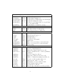
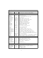
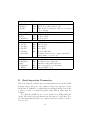
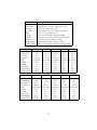
VLBA Pipeline: Outline of Data Reduction Heuristics
Gareth Hunt, Bill Cotton, & Jared Crossley
September 28, 2012
1
Introduction
The VLBA Pipeline was designed to take uncalibrated VLBA visibility data
directly from the NRAO archive and to create a file set for reingestion into
the archive or for direct use by end users. This file set contains reference
images with associated diagnostic plots, reports, scripts, and log files, plus
calibrated visibility data with associated tables. The scripts can be used to
set non-default values to processing parameters and used to repeat part or
all of the processing if the default processing is inadequate.
1.1
Scope
The scope of the present version of the pipeline is:
• VLBA data only
It may work with the inclusion of other telescopes if all of the VLBA
calibration tables are available.
• 1-15 GHz
The pipeline has been used on continuum data sets with frequencies
as high as 43 GHz with robust results.
• Calibrated fluxes
Calibration uses standard external calibration and does not include
coherence losses.
• Continuum imaging
Spectral line data sets can have the continuum calibration done but no
spectral cubes are made. Corrections based on the pulsed–cal system
may need to be turned off if this system was not used.
• Imaging including self-calibration
Multi–resolution imaging with self calibration is done.
• No polarization
No polarization calibration/imaging is currently implemented.
1
1.2
Software
The VLBA pipeline is:
• Written in python, and
• Uses Obit and AIPS tasks to do the data processing, and
• Uses AIPS data structures for intermediate data, and
• Writes FITS images and (AIPS FITAB format) calibrated datasets.
The pipeline scripts are publically available for checkout from a Subversion (SVN) repository (https://svn.cv.nrao.edu/svn/VLBApipeline).
AIPS (http://www.aips.nrao.edu/index.shtml) and
Obit (http://www.cv.nrao.edu/ bcotton/Obit.html)
are installed on all NRAO Linux computers and available for installation
via download to non-NRAO computers.
1.3
Prototype Comparison
The Mojave project was selected as an initial set of observations. This comprises more than 150 datasets, each roughly 24 hours in duration, observing
sources to track morphological changes over time. The observations are
snapshots mostly at 2cm (Ku-band) with some 3cm (X-band) observations.
This extended project has the advantage that the data have already been
calibrated and imaged by experts, and that the resultant images are publicly
available for direct comparison with the images produced by the pipeline.
The FITS images of the Mojave project are available at
http://www.nrao.edu/2cmsurvey/.
For consistency between epochs, the Mojave project necessarily has limitations on the data that they fully reduce. The VLBA pipeline has no
such limitations, and about 3500 individual images were produced from data
taken between August 2003 and December 2011. These images typically had
dynamic ranges (peak:rms) of 25-35dB. Roughly 3200 images were available
for direct comparison. The comparison was excellent. On average, the integrated fluxes for the pipeline were just over 5% lower than the images in
the Mojave catalog, as predicted.
2
2
The Process
The pipeline processing uses the following processes. Many of the default
processing parameters are frequency dependent and may be overridden and
the various steps may be turned on or off.
The following gives an overview of the processing. Details are documented in the main pipeline processing script, VLBAContPipe.py, and in
the routines called in VLBACals.py (see python online documentation). The
processing is driven by a parameter script which is initially automatically
generated but may be modified for detailed control of the processing; parameters are described in the Appendix. These are described in more detail
in the VLBA Pipeline User Manual.
1. Data retrieved from the archive
Pre-DifX data may be either multiple FITS IDI format files or a single
AIPS UVFITS data file. Data from the DifX correlator are in a single
FITS IDI format file.
2. Data converted to AIPS format
Multiple FITS IDI format files can be concatenated.
3. “Flag”
Data at low elevations and at low fringe rates are flagged using AIPS/UVFLG.
4. Initial data filtering
The data are edited with a running median window (Obit/MednFlag)
to flag deviant data such as when an antenna is late on source.
5. Standard “external” calibration
(a) 1/2 bit sampling correction
Uses AIPS task ACCOR.
(b) Parallactic angle correction
Phases are corrected for the effects of parallactic angle. Uses
AIPS task CLCOR.
(c) Ionospheric correction (TEC)
Relevant ionospheric models are downloaded from the Web and
applied using AIPS/TECOR to correct for the Total Electron
Content (TEC) given by the model.
(d) Earth Orientation Parameters (EOP)
The most recent IERS earth orientation parameters (UT1-UTC,
3
(e)
(f)
(g)
(h)
position of pole) are downloaded from the Web and used by
AIPS/CLCOR to correct the VLBA correlator model with the
“final” values.
Tsys/atmosphere/gain correction
The amplitudes are converted to Jy using measured system temperatures, standard gain curves and atmospheric opacity corrections estimated from the system temperatures. Uses AIPS task
APCAL. These gains are smoothed before application to the data.
Calibrator selection
“Calibrator” sources are then determined by doing a fringe fit on
all sources to determine which ones reliably give solid detections.
The reference antenna is picked on the basis of strong source
detections. The best calibration scan is then selected on the basis
of the fringe fit signal–to–noise estimates. This scan is the one
involving the largest number of antennas and with the highest
average SNR. Obit task Calib is used for the fringe fitting.
Pulse calibration
The pulse cal signals are used to align the phases and delays of
the various parts of the electronics. Since these are based on
phase measurements from discrete tones, the delays are ambiguous. This ambiguity is resolved using fringe fit results for the
“best” calibrator scan. Obit tasks PCCor + CLCal are used for
this.
“Manual” phase calibration
There are generally residuals delay and phase errors after correction by the pulse calibration; these are corrected using delays and
phases determined for the “best” calibrator scan and applied to
all data. Obit tasks Calib + CLCal are used for this
6. Calibration from visibility data.
(a) Initial calibrator self–calibration
All sources deemed to be calibrators are self calibrated to provide
initial images for further calibration. Phase calibration is applied
and amplitude as well if the peak in the image exceeds a frequency
dependent minimum value. Imaging uses Obit task SCMap.
(b) Delay calibration
Group delay fits are made using a fringe fit on the calibrator
sources using the source models derived in the previous step. Obit
tasks Calib + CLCal are used for the fringe fitting + correction.
4
(c) Bandpass correction
A bandpass correction for the amplitudes and phases in each
channel is determined from the best calibrator scan and the model
derived for that calibrator from the cross–correlation data. No
spectral index correction is included. Uses Obit task BPass.
(d) Calibrator phase calibration
Phase corrections on a short time scale are determined for the
calibrator sources using the source models for each. This phase
correction is then applied to the data (needed in the next step).
Obit tasks Calib + CLCal are used.
(e) Calibrator amplitude calibration
Longer time amplitude solutions are determined for the calibrator
sources. In able to prevent poor weather or other conditions at
a small number of antennas from skewing the amplitude scale,
a subset of the antennas with the most stable set of fitted gains
are used to stabilize the flux density scale. The average gain
for these antennas is divided into all gain solutions. The strong
enough calibrator sources have the solutions determined for them
applied in the calibration table. Other sources use a smoothed
version of the amplitude calibration solutions.
(f) Calibrate and average data.
Calibration is applied and the data are averaged in frequency
and possibly time. Subsequent steps use the averaged data. Uses
Obit task Splat.
(g) Self calibration of all sources
An initial self calibration to get models of all sources is performed.
Phase self–cal is always used and also amplitude self–cal if the
peak in the image is above a given threshold. Imaging uses Obit
task SCMap.
(h) Data clipping
Data with amplitudes significantly in excess of the sum of the
CLEAN components for each source are flagged.
(i) Phase calibration of all sources
The source models are used to determine the phase corrections
for all sources and these are applied to the cumulative calibration
table. Obit tasks Calib + CLCal are used.
7. Imaging and production of results.
5
(a) Imaging
Each source for which previous calibration was successful is then
imaged. This final imaging may use phase and possibly amplitude
self–calibration and the imaging uses multiple resolutions(2) to
help recover extended emission. Obit task Imager is used for the
imaging.
(b) Saving images
Final and calibration images are written to FITS files.
(c) Saving visibility data
The averaged and calibrated uv data and the tables from the
initial data are written to AIPS FITAB format FITS files.
(d) Reports
Statistics of the images are determined and an HTML page constructed to simplify viewing the results. An XML file manifest is
generated for re-ingestion into the archive.
(e) Cleanup
All AIPS data files are deleted.
3
The Products
• Calibrated (u,v) dataset with calibration and flagging tables in AIPS
FITAB format – Tables from initial data and averaged visibilities per
input dataset.
• FITS Images – one per source observed plus calibration images.
• Diagnostic plots – several per image.
• Reports and logs created during the process
• Meta-data for a VOTable to describe the products
The file set comprising all files and the meta-data are stored in a single
directory. For approved pipeline use, this directory is stored on the lustre
file system in NRAO Socorro. From there it is ingested directly into the
NRAO archive.
Sources that did not image acceptably are added to the failTargets list.
This is referenced in the HTML Report.
6
A
General Parameters
This section lists the default global parameters used in the VLBA Pipeline
scripts. They are only explained briefly, but experienced users should have
no difficulty recognizing their use and functionality. It is clearly possible to
re-run or re-start the pipeline using different values than the defaults.
Several parameters are actually placeholders for derived intermediate
products: failTarg, contCalModel, targetModel; although, in principle, contCalModel could be user-supplied. These are initialized as specified here at
the beginning of the pipeline process but may be overridden in the parameter
script.
Quantization correction
doQuantCor
True
QuantSmo
0.5
QuantFlag
0.0
Do quantization correction
Smoothing time (hr) for quantization corrections
If >0, flag solutions < QuantFlag
(use 0.9 for 1 bit, 0.8 for 2 bit)
Parallactic angle correction
doPACor
True Make parallactic angle correction
Total Electron Content (TEC) correction
doTECor
True Make TEC correction
Earth Orientation Parameters (EOP) correction
doEOPCor
True Make EOP correction
Opacity/Tsys correction
doOpacCor
True Make Opacity/Tsys/gain correction?
0.25 Smoothing time (hr) for opacity corrections
OpacSmoo
Apply phase cal corrections?
doPCcor
True Apply PC table?
doPCPlot
True Plot results?
“Manual” phase cal - even to tweak up PCals
True Determine and apply manual phase cals?
doManPCal
manPCsolInt
None Manual phase cal solution interval (min)
manPCSmoo
None Manual phase cal smoothing time (hr)
doManPCalPlot True Plot the phase and delays from manual phase cal
Special editing list
doEditList
False Edit using editList?
editFG
2
Table to apply edit list to
editList
[]
EditList
7
Do median flagging
doMedn
True
mednSigma
10.0
mednTimeWind
1.0
mednAvgTime
10.0/60.
mednAvgFreq
0
mednChAvg
1
Flag Suspect data
doFlags
True
elLim
10.0
flag0
2.0
Editing
doClearTab
True
doGain
True
doFlag
True
doBP
True
doCopyFG
True
doQuack
False
quackBegDrop
0.1
quackEndDrop
0.0
quackReason
“Quack”
Bandpass Calibration?
doBPCal
True
1
bpBChan1
bpEChan1
0
bpDoCenter1
None
bpBChan2
bpEChan2
bpChWid2
bpdoAuto
bpsolMode
bpsolint1
bpsolint2
specIndex
doSpecPlot
1
0
1
False
‘A&P’
None
10.0
0.0
True
Median editing?
Median sigma clipping level
Median window width in min for median flagging
Median Averaging time in min
Median 1=>avg chAvg chans, 2=>avg all chan,
3=> avg chan and IFs
Median number of channels to average
UVFLG editing?
Min. allowed source elevation (deg)
if > 1. flag data near zero fringe rate
Clear cal/edit tables
Clear SN and CL tables >1
Clear FG tables > 1
Clear BP tables?
Copy FG 1 to FG 2quack
Quack data?
Time to drop from start of each scan in min
Time to drop from end of each scan in min
Reason string
Determine Bandpass calibration
Low freq. channel,initial cal
Highest freq channel, initial cal, 0=>all
Fraction ofchannels in 1st, overrides bpBChan1,
bpEChan1
Low freq. channel for BP cal
Highest freq channel for BP cal,0=>all
Number of channels in running mean BP soln
Use autocorrelations rather than cross?
Band pass type ‘A&P’, ‘P’, ‘P!A’
BPass phase correction solution in min
BPass bandpass solution in min
Spectral index of BP Cal
Plot the amp. and phase across the spectrum
8
Amp/phase calibration parameters
refAnt
0
Reference antenna
refAnts
[0]
List of Reference antenna for fringe fitting
Imaging calibrators (contCals) and targets
doImgCal
True
Image calibrators
targets
[]
List of target sources
failTarg
[]
List of failed target (source,process)
doImgTarget
True
Image targets?
“ICalSC” Output calibrator image class
outCclass
outTclass
“IImgSC” Output target temporary image class
outIclass
“IClean” Output target final image class
Robust
0.0
Weighting robust parameter
Niter
500
Max number of clean iterations
minFlux
0.0
Minimum CLEAN flux density
minSNR
4.0
Minimum Allowed SNR
solMode
“DELA” Delay solution for phase self cal
avgPol
True
Average poln in self cal?
avgIF
False
Average IF in self cal?
maxPSCLoop
6
Max. number of phase self cal loops
minFluxPSC
0.05
Min flux density peak for phase self cal
maxASCLoop
1
Max. number of Amp+phase self cal loops
minFluxASC
0.2
Min flux density peak for amp+phase self cal
nTaper
1
Number of additional imaging multiresolution tapers
Tapers
[20.0,0.0] List of tapers in pixels
False
Make ref. pixel tangent to celest. sphere for each facet
do3D
noNeg
False
F=Allow negative components in self cal model
Find good calibration data
doFindCal
True
Search for good calibration/reference antenna
findSolInt
None
Solution interval (min) for Calib
findTimeInt
None
Maximum timerange, large=>scan
contCals
None
Name or list of continuum cals
contCalModel
None
No cal model
targetModel
None
No target model yet
If need to search for calibrators
doFindOK
True
Search for OK cals if contCals not given
minOKFract
0.5
Minimum fraction of acceptable solutions
minOKSNR
20.0
Minimum test SNR
failTarg
[]
list of failed sources
9
Delay calibration
doDelayCal
True
delaySmoo
None
Amplitude calibration
doAmpCal
True
Determine/apply delays from contCals
Delay smoothing time (hr)
Determine/smooth/apply amplitudes
from contCals
Stablize gains with best antennas?
Fraction of antenna to use in stabilization
List of antennas to exclude from stabilization
List of antennas to always include in stabilization
doStable
True
stableFract
0.667
[]
stableBadAnts
stableGoodAnts”
[]
Apply calibration and average?
doCalAvg
True
calibrate and average cont. calibrator data
avgClass
“UVAvg” AIPS class of calibrated/averaged uv data
CalAvgTime
None
Time for averaging calibrated uv data (min)
CABIF
1
First IF to copy
CAEIF
0
Highest IF to copy
CABChan
1
First Channel to copy
CAEChan
0
Highest Channel to copy
chAvg
10000000 Average all channels
avgFreq
1
Average all channels
Phase calibration of all targets in averaged calibrated data
doPhaseCal
True
Phase calibrate contCals data with self-cal?
doPhaseCal2
True
Phase target data with self-cal?
Instrumental polarization cal?
False
determination instrumental polarization
doInstPol
from instPolCal
instPolCal
None
Defaults to contCals
Right-Left phase (EVPA) calibration
doRLCal
False
Set RL phases from RLCal - also needs RLCal
RLCal
None
RL Calibrator source name, if given, a list of triplets,
(name, R-L phase (deg@1GHz), RM (rad/m2 ))
10
Clip excessive visibilities
doClipFlag
True Clip (flag) visibilities above sum of CCs?
clipFactor
1.25 Factor above sum of CCs to clip
clipTime
0.25 Time in min for which the data is to be averaged
before clipping
Final Image/Clean
doImgFullTarget True Final Image/Clean/selfcal
Stokes
“I” Stokes to image
True Contour plots
doKntrPlots
Final
outDisk
0
FITS disk number for output (0=cwd)
doSaveUV
True Save uv data
doSaveImg
True Save images
doSaveTab
True Save Tables
doCleanup
True Destroy AIPS files
copyDestDir
‘’
Destination directory for copying output files
empty string -> do not copy
Diagnostics
doSNPlot
True Plot SN tables etc
doDiagPlots
True Plot single source diagnostics
prtLv
2
Amount of task print diagnostics
doMetadata
True Save source and project metadata
doHTML
True Output HTML report
B
Band-dependent Parameters
This section lists the default band-dependent parameters used in the VLBA
Pipeline scripts. They are only explained briefly, but experienced users
should have no difficulty recognizing their use and functionality. It is clearly
possible to re-run or re-start the pipeline using different values than the
defaults.
Note that the VLBA has two receiver bands below 1GHz (90cm and
50cm). The band-dependent parameters are the same for both bands. Note
also that 9mm (Ka) is included for completeness in the software, but there
is no receiver.
11
Parameter
manPCsolInt
manPCSmoo
delaySmoo
bpsolint1
FOV
solPInt
solAInt
findSolInt
findTimeInt
CalAvgTime
Description
Manual phase cal solution interval (min)
Manual phase cal smoothing time (hr)
Delay smoothing time (hr)
BPass phase correction solution in min
Field of view radius in deg.
phase self cal solution interval (min)
amp+phase self cal solution interval (min)
Solution interval (min) for Calib
Maximum timerange, large=>scan
Time for averaging calibrated uv data (min)
Parameter
manPCsolInt
manPCSmoo
delaySmoo
bpsolint1
FOV
solPInt
solAInt
findSolInt
findTimeInt
CalAvgTime
<1GHz (P)
0.25
10.0
0.5
10/60
0.4/3600
0.10
3.0
0.1
10.0
10/60
Parameter
manPCsolInt
manPCSmoo
delaySmoo
bpsolint1
FOV
solPInt
solAInt
findSolInt
findTimeInt
CalAvgTime
2cm (Ku)
0.5
10.0
0.5
10/60
0.05/3600
0.25
3.0
0.5
10.0
10/60
20cm (L)
0.5
10.0
0.5
15/60
0.4/3600
0.25
3.0
0.25
10.0
10/60
1cm (K)
0.2
10.0
0.5
10/60
0.05/3600
0.25
3.0
0.3
10.0
5/60
12
13cm (S)
0.5
10.0
0.5
10/60
0.2/3600
0.25
3.0
0.25
10.0
10/60
9mm (Ka)
0.2
10.0
0.5
10/60
0.04/3600
0.25
3.0
0.2
10.0
5/60
6cm (C)
0.5
10.0
0.5
10/60
0.2/3600
0.25
3.0
0.5
10.0
10/60
7mm (Q)
0.1
10.0
0.5
5/60
0.04/3600
0.1
3.0
0.1
10.0
5/60
3cm (X)
0.5
10.0
0.5
10/60
0.1/3600
0.25
3.0
0.5
10.0
10/60
3mm (W)
0.1
10.0
0.5
5/60
0.02/3600
0.1
3.0
0.1
10.0
4/60