Download 2 Theory - Larsengelsby.dk

2
Aalborg University Copenhagen
Semester: 1. semester
Title: WebGIS solution for wastewater facilities in Denmark
Theme: GI Technology and Information System
Project period: 2012 September 2th – 2013 January 8th
Submission date: 2013 January 8th
Abstract
Supervisor: Morten Fuglsang
This project concerns creation of
web application by adequate
searching possibility for
wastewater in whole Denmark
where we added several
functionalities with advanced
search options. We identified two
kinds of user groups who will use
the application. These groups are:
the professional and the citizens.
We structured our project work by
following agile method. We used
different kinds of platforms for the
project like python programming,
PostGreSQL, OpenLayers, GeoExt
etc.
Project group: 2
Attendees:
_________________________________________
Lars Kristian Engelsby Hansen (20120573)
_________________________________________
Vlad Hosu (20120203)
_________________________________________
Meherun Nahar (20111794)
_________________________________________
Thomas Hallundbæk Petersen (20093521)
Number of copies: 7 copies
Number of pages: 84 pages
In appendices: 62 pages
Copyright © 2012. This report and attached material cannot be published without the authors’ written acceptance.
3
4
Preface
This project is drafted by project group which consists of four students from Aalborg University.
The project is emanating from the theme GI Technology and Information System and is developed in the
period of September 2th 2011 to January 8th 2013. The project is furthermore written based on the M.Sc.
Programme in Geoinformatics study guide for 7th semester.
In the project period the courses, Spatial Data Infrastructure and Geospatial Information Technology, has
introduced us to databases, programming and Web GIS. Decisions about which programs to use have been
based upon experienced gained during these courses.
The project group’s main supervisor is Morten Fuglsang at Aalborg University.
5
Reading advice
The reading advice is prepared to simplify the flow for the reader through the report
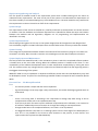
Source references
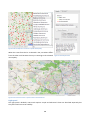
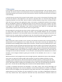
The Chicago referencing style is used to source our references. It is an author-date system that consists of
two parts: the citation in the text and a bibliography at the end of the report. The authors surname and the
year of publication appear in the citation in the text. The author’s surname, other names as initials, year of
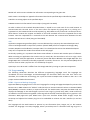
publication, title, edition and place of publication are shown in the more detailed bibliography. Figure 1
shows how the source references are managed in the citation in the text and the bibliography.
Figure 1: Examples of the Chicago method, to the left is seen the citation within the text and to the right the text in the
bibliography (Murdoch University 2011)
Character references
References to figures, tables, code samples and appendixes are used in certain ways. They are numbered
sequentially from the start. For example figure 1 in the text refers to a figure identified as Figure 1. Tables
and code samples are referred to as figures. Appendixes are referred to with continuous numbers.
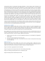
Lists of Abbreviations
API
Application Programming Interface
CGI
Common Gateway Interface
CSS
Cascading Style Sheets
DBMS
Database Management System
DCL
Data Control Language
DDL
Data Definition Language
DML
Data Manipulation Language
ECMA
European Computer Manufacturers Association
6
EPA
Environmental Protection Agency
HDBMS
Hierarchical Database Management System
HTML
Hypertext Markup Language
HTTP
HyperText Transfer Protocol
JSON
JavaScript Object Notation
NDBMS
Network Database Management System
ODBMS
Object-oriented Database Management System
OGC
Open Geospatial Consortium
ORDBMS
Object Relational Database Management System
PHP
Personal Home Page tools
RDBMS
Relational Database Management System
SLD
Styled Layer Descriptor
SQL
Structured Query Language
SQL
Structured Query Language
URI
Uniform Resource Identifier
URL
Uniform Resource Locator
WFS
Web Feature Service
WMS
Web Map Service
WWW
World Wide Web
XML
Extensible Markup Language
Appendix
In addition to the report an appendix is presented. The appendix intended to substantiate the facts written
in the report. Each appendix is numbered and can be found in the contents of the appendix
7
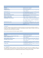
Content
Preface .................................................................................................................................................. 5
Reading advice....................................................................................................................................... 6
Source references............................................................................................................................... 6
Character references........................................................................................................................... 6
Lists of Abbreviations .......................................................................................................................... 6
Appendix ............................................................................................................................................ 7
Content ................................................................................................................................................. 8
1 Introduction ...................................................................................................................................... 10
1.1 Problem Statement ..................................................................................................................... 10
1.2 Report structure.......................................................................................................................... 11
2 Theory .............................................................................................................................................. 13
2.1 System design strategies.............................................................................................................. 13
2.2 Database management system (DBMS) ........................................................................................ 17
2.3 Web Architecture ........................................................................................................................ 22
2.4 Programming .............................................................................................................................. 26
2.5 Web based GIS............................................................................................................................ 32
2.6 Cartography theory ..................................................................................................................... 43
3. Methodology ................................................................................................................................... 47
3.1 System design ............................................................................................................................. 47
3.2 Implementation .......................................................................................................................... 49
3.3 Data ........................................................................................................................................... 56
4 Result ............................................................................................................................................... 65
4.1 Functionality ............................................................................................................................... 65
4.2 Design ........................................................................................................................................ 72
5 Discussion ......................................................................................................................................... 74
5.1 Data ........................................................................................................................................... 74
5.2 Servers ....................................................................................................................................... 75
5.3 Application ................................................................................................................................. 75
5.4 Agile vs. waterfall ........................................................................................................................ 76
5.6 Answering research questions...................................................................................................... 77
6 Conclusion ........................................................................................................................................ 79
7 Perspectives...................................................................................................................................... 80
8
7.1 Designing the map....................................................................................................................... 80
7.2 Access to more data .................................................................................................................... 80
7.3 Improve the performance and interoperability ............................................................................. 80
7.4 Shortcomings of the application ................................................................................................... 81
Bibliography ........................................................................................................................................ 83
9
1 Introduction
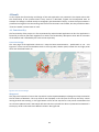
WebGIS, which is a combination of web and geographic information systems, has grown rapidly after its
origin of development in 1993 (Fu and Sun 2011). From then it gained huge popularity as people can use
GIS from the web. The internet browsers have access to GIS applications without buying software , while
map services allow GIS applications without hosting them locally to have the latest updates. Often a client
has open access to filtered data. This semester we decided to conduct a project on webGIS application. The
purpose of the work is to create a webGIS solution for wastewater with the possibility to search f rom
different perspectives, such as geographical searches and searches on specific measured parameters .
Therefore, we chose wastewater data in Denmark. The data is an extract from the database called WinSpv
containing data about wastewater from Danish wastewater facilities. The data is used for various tasks
regarding wastewater governance (WM-data 2006). WinSpv is an older database and it is required that
each wastewater facility report analysis on a number of compounds a number of times every year.
‘Compound’ is a word that will be used throughout the report. It is used as a common word for chemical
substances measured in wastewater. All data is collected in a database. The age of the database is for
instance visible in the municipality codes which still follow the old municipality numbers.
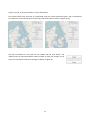
Our extract contains data from January 2012 until November 2012. Each time a sample is made on a
facility, measuring one compound there is one row. We have more than 58.600 samples (rows) spread on
721 wastewater facilities all over Denmark (excluding Bornholm).
Data in WinSpv is divided in an administrative part and a data part. The local municipality is responsible for
keeping the administrative part updated. The administrative part includes information about the facility.
The data part includes information about measurements of different compounds on the local facility. This
part is updated locally at the facility, but the municipality is responsible for verifying the data. This division
in responsibility is available in “Dataansvarsaftalen for punktkilder” which is approved in a partnership
between the Danish EPA, Local Government Denmark (KL) and Danish Regions. (Danish Environmental
Protection Agency 2011)
Each record has two coordinate sets. One for the wastewater facility – referred to as “in” – and one for the
corresponding point of discharge. There are no data for the pipe between the two points but a straight line
between the two corresponding point will be able to illustrate the connection.
The system is meant to be public because data is not linked to any privacy restrictions. However users with
a professional or interest for wastewater are most likely to use the web application. These are people that
have some knowledge about the data. Primary professionals working with Wastewater are the target
group.
1.1 Problem Statement
In this report we want to test the possibilities of making a WebGIS application by designing it in order to
interactively display and make searchable wastewater facilities and their measurements. By creating such
an application it is possible to spread knowledge and information easier. Clients who need wastewater
facility related knowledge can get their required data by searching. Moreover WebGIS application will help
for further research facilities. With these thoughts in our minds, we decided our problem statement to be:
10
How can an open source WebGIS application be designed in order to interactively display and make
wastewater facilities and their measurements searchable?
To make the problem statement more concrete we made three research questions which will further guide
us to follow the appropriate way. The three research questions are:



What types of functions could be developed to support the use of the data in the application?
How can data be gathered, refined and stored to fit into the application functions?
Which platforms should be used in the application?
1.2 Report structure
Our report consists of following sections:







Introduction
Theory
Methodology
Result
Discussion
Conclusion
Perspectives
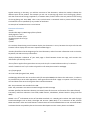
We conducted out report by following three phases:
Figure 2: Structure of the report
Phase 1 describes about the project. It consists of an introductory part and theory section. In th e
introductory part we describe the background of the project. It is followed by a problem statement and
three research questions and limitations that we face while conducting the project. To better understand
the project some information and theory is needed. In our report we discuss system design strategies,
theory on database management systems, web architecture, programming languages and web based GIS.
This section will give understandings of different concepts used.
Phase 2 is where data preparation and methods are discussed. In the methodology section we describe our
system design, database structure design and user requirements for the project. Then we discuss the
implementation process where we discuss system implementation and user interface design. This phase
also includes the methods we follow in the implementation. Next we present our results by using web
applications and taking some screenshots of the outputs.
11
The last phase of the report is discussion and evaluation phase which contains discussion and conclusion. In
the discussion part we discuss the choices and outputs from the choices. It also includes the shortcomings
of the work. In the conclusion part we answer our three research questions and in the end we look at the
project perspectives.
12
2 Theory
In this chapter, an introduction to the theoretical aspects of the project will be presented. We will have a
look into different system design strategies. Afterwards we will focus on describing the underlying pillars of
the theoretical aspects in the project.
2.1 System design strategies
In the following section two system design strategies is discussed. The two methods are: the waterfall and
the agile methodologies. The strategies are needed to make the process more functional and to perform in
a better way. The strategies also lower cost including time and money. Two strategies which will be
discussed in the following section have pros and cons which will also be considered.
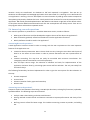
The waterfall method
In the waterfall software development, all the requirements are gathered at the beginning which is
followed by a design and implementation phase. It is a sequential and phase wise method that does not
leave opportunity for going back and revisiting all the requirements. It was first introduced in 1970. The
waterfall method is a linear and sequential approach in which separate teams are appointed in each stage
to ensure greater project and deadline control.
The project team first analyses, then determines and prioritizes business requirements / needs. In the
design phase business requirements are translated into IT solutions, and a decision taken about which
underlying technology i.e. COBOL, Java or Visual Basic, etc. is to be used. Once processes are defined and
online layouts built, code implementation takes place. The next stage of data conversion evolves into a fully
tested solution for implementation and testing for evaluation by the end-user. The last and final stage
involves evaluation and maintenance; with the latter ensuring everything runs smoothly (Buzzle 2012).
Figure 3 General Overview Waterfall model (Buzzle 2012)
The goal of the model is to fulfil every step 100 % unless one cannot proceed to the next step.
The steps in the model are described below:
13
Requirement gathering and analysis
The first phase of waterfall model is the requirement phase which includes meeting with the clients to
understand their requirements. The most crucial part of the system is to understand the requirements of
the clients carefully as misunderstandings may raise validation errors. The team should be very careful with
the requirements so that in the end it can fulfil all the requirements.
System Design
The requirements of the clients are studied very carefully and these are broken down into several sections
or modules. Then the hardware and software requirement are identified to follow the steps. Interrelation
between the modules and the algorithms, diagrams etc. all programming and implementation are
identified in this step.
System Implementation
Actual coding is taking place in this step. In the system design phase all the algorithms are designed and
here a software program is written based upon them and the codes written for every module are checked.
System Testing
In this stage the implemented software modules are tested and if there exists any bugs or errors these are
corrected in this step. After the code is rewritten it is tested again until the desired output is achieved.
System Deployment and Maintenance
The final phase of the waterfall model, is the maintenance phase in which the completed software product
is handed over to the client after testing. When the software product is handed to the client it is the
responsibility of the software development team, to take maintenance responsibility by visiting the client
site. If a customer wants any changes then the system has to follow the steps from the beginning which is
the biggest shortcoming of the system.
Waterfall model is easy to implement. It depends on different phases thus this interdependency may lead
to development issues. In spite of the shortcomings waterfall model is accepted all over the world (Buzzle
2012).
Pros and Cons – The Waterfall method
Pros
- The linearity makes it simple and low cost to implement.
- A great advantage is that every stage is easy to document; this makes the designing phase easier to
understand.
Cons
-
There is no turning back, if something in the requirement or design step went wrong. It can be
complicated to smooth out in the implementation step
If the client you work for comes up with additional requirements to the software, it can cause a lot
of confusion. Additionally the environment can change also leading to new requirements.
Changes made later in the completed software, can result in a lot of problems.
The biggest drawback is that there is no working system until the final stage of the development is
over. So it is not possible for the client to make comment in the process, or even check if t he
system meets the requirements (BuzzleB 2012).
14
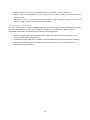
Agile methodology
Like waterfall, the agile methodology is also used in software development. It is an alternative to traditional
project development. It follows iterative work flows in the response of unpredictability of software building
(AgileMethodology 2012).
Dr. Winston Royce mentioned some issues regarding traditional software development in a paper entitled
“Managing the Development of Large Software Systems,” in 1970. He presented that projects could be
developed in a sequential basis. Developers first fulfil all the requirements then carry out every phase. But
due to some shortcomings of the traditional system in February 2001, 17 software developers decided to
make new methods for software development. They were agreed on agile methodology and they published
the manifesto for agile software development (AgileMethodology 2012).
Agile manifesto includes 12 principles:












Our highest priority is to satisfy the customer through early and continuous delivery of valuable
software.
Welcome changing requirements, even late in development. Agile processes harness change for
the customer's competitive advantage.
Deliver working software frequently, from a couple of weeks to a couple of months, with a
preference to the shorter timescale.
Business people and developers must work together daily throughout the project.
Build projects around motivated individuals. Give them the environment and support they need,
and trust them to get the job done.
The most efficient and effective method of conveying information to and within a development
team is face-to-face conversation.
Working software is the primary measure of progress.
Agile processes promote sustainable development. The sponsors, developers, and users should be
able to maintain a constant pace indefinitely.
Continuous attention to technical excellence and good design enhances agility.
Simplicity--the art of maximizing the amount of work not done--is essential.
The best architectures, requirements, and designs emerge from self-organizing teams.
At regular intervals, the team reflects on how to become more effective, then tunes and adjusts
its behaviour accordingly (AgileManifesto 2012).
15
Figure 4: Development Methodology of Agile Approach
If any project has very little planning in the beginning, Agile approach can be a good method to choose for
the project. As it is mentioned earlier, Agile is an iterative process so there is plenty of opportunity for
changes. The basic idea is that working with codes by doing iterations it is possible to develop additional
functionalities in the system. The work cycles are short. If the cycle does no t work then one can follow
another cycle as the process is not too long. The main advantage of these methods is that if something is
wrong one can start again a new approach. It opens a door for communicating with all the members in the
project including development team, project leader and clients. In the development process it is possible to
change as the method is more flexible (AgileMethodology 2012).
The agile methodology provides many opportunities for software development throughout the
development lifecycle as it follows iterations of the cycle. In the agile approach every aspect of the
development – requirements, design etc. is followed in every cycle, and if the project is stopped then there
is a possibility to follow it in another direction. Here the development teams have many chances to reach
the goal, while in Waterfall methods the development teams have only one chance to reach the goal. Agile
16
methods reduce both development costs and time to market. The development methods help companies
to build the right product (AgileMethodology 2012).
Pros and Cons – The Agile methodology
Pros
- Delivers value fast (fist iteration/work cycle can be demonstrated)
- High flexibility
- No significant rework
- Product is tested early, because of the short iterations
- Risk decreased by always having working software
- Good if end state is unknown
Cons
-
May lead to unrealistic expectations
Not process orientated, which can lead to the lack of documentation
Though there are pros and cons for both the two strategies, Agile methodology is used widely when the
developers are not aware of the whole process and need to start from the previous step again while
Waterfall method does not give such kinds of opportunity.
2.2 Database management system (DBMS)
A database is a collection of one or more data files which has integration, linkages and cross reference with
each other. The main advantage of database is that they can be easily organized. Software called a
database management system (DBMS) is used to retrieve data. Normally DBMS, which is a crucial
component of most successful GIS, are used to store, manipulate and retrieve data from a database files
that allow users to create, edit and update. It is also possible to add, delete, change, sort or search in
DBMS (Longley 2004).
Fundamental characteristics of DBMS
Database will serve all kinds of individual rather than a single individual. There are some fundamental
characteristics of DBMS are described below and these factors enhance the efficiency and productivity in
data management.




The method of data storage can be considered independently of the programs that access the
database.
A controlled and standardized approach to data input and update can be enforced, with
appropriate validation checks to ensure data integrity and consistency between data files.
Security restrictions on access to specific data subsets can be applied.
A consistent approach can be adopted for managing simultaneous multi-user read and update
operations on specific files or tables (Longley 2004, 252)
DBMS reduces data redundancy. Therefore, the maintenance cost of data is low as it decreases data
duplication by storing data in one place. Many users can use database management systems that help to
improve the management the system and thus can transfer user knowledge to the system. In DBMS data
security is highly established. The biggest advantage of DBMS is to maintain standards and security. It helps
17
to make files more consistent to manage data in an easier way when multiple programmers are involved.
Data is easier to access and manipulate through it. It also reduces the reliance of individual users on
computer specialists to meet their data needs. DBMS allow multiple users to access the same data
resources. Though users are benefitted this way, there arise some security risks due to it. It is neces sary to
protect some information. Through the use of passwords, database management systems can be used to
restrict data access to only those who should see it (Longley 2004).
On the other hand, DBMS has some disadvantages. The initial cost of acquiring and maintaining DBMS
software can be high and in some cases DBMS can be complex in data management. The implementation of
DBMS system can be expensive and time consuming. For large organizations, training requirement alone
can be very costly (Longley 2004).
Types of DBMS
There are four structural types of database management systems: hierarchical, network, relati onal, and
object-oriented.
Relational Database Management System (RDBMS)
In the relational databases, data is connected in different files by common key field. In the relational
databases, data is stored in different tables, having uniquely identified key fields. Each relation is composed
of tables, attributes or fields. It is not necessary for the users to know how the data is stored in the system
because data exists independently in a relational database. In relational databases, tables or files filled wi th
data are called relations and columns are referred to as attributes or fields. A Relational Database
Management System (RDBMS) is a software program used for data creation, maintenance, modification,
and manipulation in a relational database. Relational databases are more flexible than any other databases
(Longley 2004). The relational database is popular due to two reasons. Relational databases do not require
training. They can be used with little or no training. Another reason is that database entries can be
modified without redefining the entire structure. The disadvantage of this method is that it takes more
searching time for data than if other methods are used. The relational DBMS is the dominating DBMS
(Anfindsen 1993, 41), even though this source is quite old, and the world of databases moves fast, this
statement is still relevant.
Hierarchical Database Management System (HDBMS)
The hierarchical DBMS gets its name from the fact that it stores data hierarchically in tree structures. The
rules are, that every node in the tree can have several children but only one parent, and that only one -toone or one-to-many relations downwards in the tree are allowed (Balstrøm, Jacobi and Bodum 2006, 144).
This way of ordering data is well known from way files are saved in folders and searched in for example
windows browser. A folder can have a number of subfolders which can have a number of files, but a file
cannot be in two folders at the same time, without being actually copied and thereby having redundancy.
Network Database Management System (NDBMS)
The network DBMS has a lot of similarities with the HDBMS. The difference is that here, children can have
more than one parent, so it opens up for many-to-many relationships (Balstrøm, Jacobi and Bodum 2006,
144). With this feature, some redundancy can be eliminated by not forcing the same information in more
branches, but instead the information having several parents.
18
Object Oriented Database Management System (ODBMS)
The object-oriented DBMS is both newer and more immature than the other three mentioned DBMS types
(Anfindsen 1993, 42). It follows the structure of the object-oriented programming and includes classes,
subclasses and objects, with inherited properties. According to Balstrøm, Jacobi and Bodum (2006, s.156)
the ODBMS has great unutilized potential, and they are well suited for some spatial data, because a lot of
spatial information, and metadata is inherited.
Basic elements of a database
In this subsection basic elements in databases and relational databases in particular are described. This is
done in order to lay the ground for the use of the terminology later on.
Tables
Tables can be described as the data containers of relational databases. They have a number of fields and a
number of entries usually represented in a matrix like figure 5.
Figure 5 - Example table
In the example in figure 5, there are three entries, corresponding to three people, with matching
information, meaning Tom is 25 years old, and has ID 1. There are three types of information about these
people called fields. A database can contain several related tables.
Views
A view is a dynamic representation of data, a ‘window’ of the data so to speak (Date 2004, 73). While a
view will look like a table, they differ from tables by not being stored as data, but rather as queries on one
or more tables (ibid.). Because views are dynamic and light in data storage they can be used for splitting up
advanced or extensive queries.
Indices
An index is a data structuring that is used to speed up searching in data on a table (Balstrøm, Jacobi and
Bodum 2006, 138). Indices are not visual to the user, and in that way they can be seen as maps of the data
for the computer to find its way through the data. Indices are created on one or more columns in order to
speed up searching information in these. Likewise a spatial index can be created on the geometry of a
spatial database. This can help to speed up spatial queries and visual displaying of spatial data.
19
Normalization
The design of a database may not always be straight forward. Normalization is a way of making sure data in
a relational database is arranged with the least possible amount of redundancy, and making sure change is
easily manageable (Balstrøm, Jacobi and Bodum 2006, 151).
Normalization is a stepwise approach of rearranging data, first achieving 1st normal form through 3rd, 5th or
even 6th normal form depending on the source. According to Balstrøm, Jacobi and Bodum (2006, s.151)
normalization is not an objective science and databases are often seen as being normalized when 3 rd
normal form is achieved. On the other hand, lots of sources describing the importance of higher degrees of
normalization could be found.
The greater the size of a database, the more important normalization is (Balstrøm, Jacobi and Bodum 2006,
151). Normalization of only the first three normal forms will be discussed.
1st normal form
For a database design to achieve first normal form, the database must have a unique and unambiguous
primary key, so that each entry can be uniquely identified for each record. There must also not be repeated
groups (Balstrøm, Jacobi and Bodum 2006, 151-152), which means that a column of properties cannot
contain two or more properties for one entry, like a book having more than one author. This should instead
be described in a distinct table, in order to achieve 1st normal form.
2nd normal form
The 2nd normal form is achieved if the first normal form is achieved, and if a column does not only describe
part of the primary key. This is only problematic if the primary key consists of more than one column
(Balstrøm, Jacobi and Bodum 2006, 152). Let us say the table achieving the first normal form with the
authors, has book and author combined as primary key. In this case, a column about the date of birth of the
author, which is only describing part of the primary key, would violate the 2 nd normal form. Then a third
table would need to be generated with information about the author, with only an author id or author
name as primary key.
3rd normal form
The 3rd normal form is achieved if the 2nd normal form is achieved, and if no columns describe non primary
key columns (Balstrøm, Jacobi and Bodum 2006, 152). Let us say that the books from the previous example,
contains information about the publisher. This is ok, but if another field describes the publisher address, or
publisher phone number, another table must be created to include this information, as it describes a non
key column.
Structured Query Language (SQL)
SQL is a database language that manages mainly database management systems (RDBMS). SQL are
combinations of commands, clauses, expressions, predicates, and options. The three most used SQL sublanguages are:
Data Definition Language (DDL)
 Creation and modification of relational schema
 Schema objects include relations, indexes, etc.
Data Manipulation Language (DML)
20
 Insert, delete, and update rows in tables
 Query data in tables
Data Control Language (DCL)
 Concurrency control, transactions
 Administrative tasks, e.g. setup of database users, security permissions (Balstrøm 2012)
SQL supports logical data model concepts, such as relations and keys. It can express common data intensive
queries.
Listed below are some examples of typical SQL functionality:
 Select distinct
Distinct selections are used to make sure only unique elements are selected. This is only relevant in
non-key only selections.
 Join
A Join is a combination of two or more tables (tables can also be joined with them self). This makes
it possible to display and compare columns from different tables. This is usually done by a common
field in the two tables, so that the information is combined in a meaningful way.
 Full-join
Full joins are like joins except joins only keeps records with matches. So full joins can have NULL
values where there are no match, where this will not be an entry in the join.
 Sql-functions
In sql it can be helpful to change datatypes. For this the CAST function can be used.
CAST(integer_column AS text)will convert integers in a column to text strings.
Also aggregate functions can be useful. These can be used to select the newest date, summarize
data, count occurrences, get average number and more.
 Union
Tables can be added together using union. If two tables are united all records from the two tables
will be put in to one big table, with the combined number of entries, except for duplicate values
that is, to include duplicate values union all can be used.
PostGreSQL 9.2
PostGreSQL is an open source object relational database system (ORDBMS). It runs on all major operating
systems, including Linux, UNIX (AIX, BSD, HP-UX, SGI IRIX, Mac OS X, Solaris, Tru64), and Windows.
PostGreSQL itself follows standards supporting complex queries, triggers, backup and views among
database features. Its SQL implementation conforms to the ANSI-SQL: 2008 standard. The software can be
easily extended by adding different functions. It has native programming interfaces for C/C++, Java, .Net,
Perl, Python, Ruby, Tcl, ODBC etc. (PostGreSQL 2012).
The PostGresSQL uses a server process and the user client`s applications request:
 A server process: It performs database actions from the client side and accepts the connections to
the database from the client applications and thus manages database files.
 The user client’s applications request: Client applications can be very diverse (e.g. a text-oriented
tool, graphical application, web server, or a specialized database maintenance tool). Some client
21
applications are supplied with the PostGreSQL distribution, but most of them are developed by the
users.
A typical client/server application is typically on different hosts which must communicate via Internet. The
software can handle multiple connections and therefore the master server is always opened to run client
requests for a connection. We use the PostGreSQL as our database management system, and let the
PostGreSQL database load data to the server (GeoServer). For this purpose, we install an application called
PostGIS to the software. It is an application which makes PostGreSQL support geographical data.
PostGreSQL is a well-established database program; the first Postgre95 release 0.01 was released the 0105-1995. The 9.2.1 version was released at 24-09-2012, and is a stable version working on desktops with
Windows 7 OS (PostGreSQL 2012).
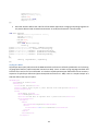
2.3 Web Architecture
In the following section the most important components of the webGIS will be discussed. Clients and
servers are the two components where the interaction is necessary. Clients send requests to the servers
and servers responds to it. HTTP acts as glue between the client and server.
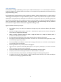
Client/Server
The client/server model is an approach to computer network programming. The approach assigns either
the client role or the server role to a computer in a network. The server is a computer that share s its
resources. The client is a computer that creates contact to a server in order to make use of the resources
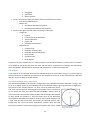
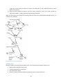
from the server. In figure 6 is an example of the client/server model. In the example the internet
intermediates the connection between the clients and the server. (Fu and Sun, 2011)
The internet is not necessarily always the connection between servers and clients. It can be on a local
network between computers as the clients and a printer as the server.
Figure 6 – The relation between clients and servers
In web application more servers can be used to fulfil the requirements of the server. A basic workflow of a
web application is as follows (Fu and Sun 2011):
22
A user initiates a
request. Typically
through a browser
The web server
receives the request
and returns a result
through the
internet etc.
The user receives
the response
through its client.
Figure 7 – Workflow of a web application
On the server side programming languages as Java, PHP, Python or VB etc. is doing the work. They are
responsible for accepting requests from the clients and serving clients with responses.
The most popular client type is the Web browser client. Among other types of clients FTP, IMAP and SOAP
clients can be mentioned (Fu and Sun, 2011). The web browser client is a software application for retrieving
and presenting information resources from a server on the Web. The web browser is called the “face of the
Web”. On the technical side, the browser has implemented HTML specifications so it knows how to
communicate with the Web servers. While Web browsers differ regarding implemented software,
differences in performance and compatibility may happen.
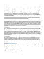
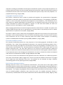
Thick client (Client side processing of data)
Clients interact with the data and other GIS services through the internet. Thick client architecture relies
mostly on the client beyond servers to perform any functions accomplishing by a web browser or a native
client application. Here the client performs most functions. Client side applications allow the thick client to
request the source data from the server. When the server processes, requests and sends information, the
client renders maps and performs analysis. In this architecture the server does not perform all the tasks. It
sends downloadable GIS capabilities and data is processed in the user’s computer. An example illustrated in
Figure 8: Example of a client side strategy
Client side architecture follows some steps. First they send a request to the server. Then the server
processes the request and returns information and data. Then data is processed on the user’s computer.
Due to several advantages client side strategies are good. Clients can interact very fast with the server.
Data resides and processes locally. The users posses the controlling power of data handling.
When users send requests to the server and get the response, they can work with the data immediately.
Again it minimizes pressure on the server as only few tasks are performed there (Fu and Sun 2011).
But client side strategies have some disadvantages also. This strategy is sometimes time-consuming.
When the user sends requests for large amounts of data, it takes time to send the requested data by the
server. If the server sends complex data, sometimes, it is very difficult to process that datasets from the
client’s side unless it is not powerful and it makes the system very slow. The user needs adequate training
to process complex datasets. On the other hand, internet bandwidth and client computing power hampers
the tasks. The server cannot send gigabytes of data over internet to perform GIS operations (Fu and Sun
2011).
23
Figure 8: Example of a client side strategy (Foote og Kirvan 2012)
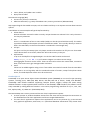
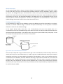
Thin client (Server side processing of data)
Server side strategies allow performing most of the tasks by the servers while client do less of the job.
Users simply send requests to the server via internet and server does the processing through map
generation and analyzing data. It returns a response to the client with the output information. The client’s
browser displays the result/information.
Server side architecture follows these steps: First the client sends request to the servers. Then the server
processes requests and sends information. Then the output required by the client is returned to the server
and send response to the client. The last step is that client can see the information is their browser.
Server side strategies have some advantages. There is less work for the users to perform. The user needs
only a Web browser to perform the task. Any other software is not needed here to install from the user
side. Most of the tasks are processed in the server, so the client does not need to have a powerful
computer. On the other hand, it has some bottlenecks also. The servers always stay in pressure due to the
lots of requests. Interaction with the user is very limited as the interface is build with HTML and JavaScript
which is not compelling with the user interaction (Fu and Sun 2011).
Figure 9: Example of server side strategy (Foote og Kirvan 2012)
24
The division of the tasks between thin and thick client
Due to the advancement of technology both the server side and client side strategies are becoming more
and more powerful and can take greater workloads. Figure 10 Distribution of tasks of the very thin and
thick layer and how it can be best practiced shows different task divisions, between the server and the
client in a best possible way. In the very thin client architecture, most of the GIS activities are performed by
the server, while the opposite scenario is seen in case of very thick client architecture. The best practice
recommends that base maps, query and analysis are done by the server while client may handle
operational layers.
Figure 10 Distribution of tasks of the very thin and thick layer and how it can be best practiced (Fu and Sun 2011, 41)
HyperText Transfer Protocol
HTTP is the main way to link web clients and web servers by exchanging files between the web browser and
web server. As a message carrier HTTP carries user requests from browsers to servers and takes the
requested information (text, graphic images, sound, video and other multimedia files) from servers back to
browsers. To communicate between the web client and web server it uses different commands or
methods. Each Web Server has an HTTP domain to listen to HTTP requests from the web browse r. When
HTTP daemon receives the request, it processes the request based on some standard methods. These
methods include GET, HEAD, PUT, POST, REPLY etc. (Peng and Tsou 2003).
GET is the most commonly used method in retrieving whatever data are identified by the URL, including
running scripts. It is also used for searches.
HEAD represents only the HTTP headers not including the actual document body.
PUT stores the data to the supplied URL in the Web server. The URL must already exist. POST and REPLY
should be used for creating new documents.
25
DELETE will ask the server to delete the information corresponding to the given URL.
POST creates a new object or appends information linked to the specified object identified by a URL.
LINK links an existing object to the specified object.
UNLINK removes link information from an object. (Peng and Tsou 2003)
As HTTP includes all the methods described above, it would be an easier task for the web browser to
communicate with the web server. If the user enters file requests by typing URL or by clicking on a
hypertext link, the browser builds an HTTP request (e.g., GET, HEAD or PUT) and sends it to the web server.
HTTP daemon receives the request and based on the HTTP methods returns the requested file to web
browser. Once the requested file is returned to the web browser the communication between the web
browser and web server is done (Peng and Tsou 2003).
API
Application Programming Interface (API) is a service delivered by a company who wants developers and
users to build applications on top of their product. (Gosnell 2005) refers to companies as Google, eBay,
Amazon, MapPoint and FedEx who have open APIs. This is developed to ensure that website developers
easily can incorporate the content from the API to the web pages.
Technically speaking it is a protocol that allows some software to interact with another piece of software.
When accessing an application that contains one (or more) API, the API makes a call to its origin, which
returns a result inside the application. A commonly known API within WebGIS is the Google Maps API. The
Google Maps API is a free API, and widely supported in tutorials, forums etc. This is by Gosnell (2005) called
the main issue to make a popular API – the availability of support.
OpenLayers is an API as well. It differs from the Google API due by having an open source approach.
2.4 Programming
The following subsection describes the different programming languages used. The languages are
introduced and their advantages and disadvantages are discussed. Other than that their basics are
described, this includes the terminology, the syntax and some examples with relation to their use in t he
project are described and commented.
HTML - Hypertext Markup Language
Hypertext Markup Language which is the main language for creating web pages developed by scientist Tim
Berners-Lee in 1990. HTML is the "hidden" code that helps us communicate with others on the World Wide
Web (WWW). It contains contents, a layout and format. The web browser interprets the HTML code and
displays the webpage in the web designer`s point of view. Tags (e.g. head, body, table, center and fonts)
are added in the text while writing HTML. These tags tell the browser how to display text or graphics in the
document. Web pages with pure HTML have a plain user interface. HTML allows images, scripts like
JavaScript and objects like browser plug-ins to be embedded to enhance the user interface (Fu and Sun
2011).
The language tells the web browser to present lay out information (text, images, etc.) in the browser
window. The language is a markup language, where you markup text in a document with tags to giv e it a
26
special meaning. In that way, you add the structure of the document, where the markup indicates the
different parts of the product. For example you can use an opening tag <html> and a closing tag </html>
with the content that the tag is applied to, in between them, and the slash is the only marker of the closing
of the tag (Peng and Tsou 2003). Like a tree, each element is contained inside a parent element, where
each element can be specified by any number of attributes.
An example of a HTML structure is seen below:
Document Structure:
<html>
<head><title>My First Web Page</title></head>
<body bgcolor="red">
<h1>This is a header </h1>
<p>A Paragraph of Text</p>
</body>
</html>
This markup allows letting a web browser display the document in turns, because the script tells the web
browser how to display this structure. Important HTML Tags is:
<head></head>found at the beginning of an html document, and will contain information such as the title,
keywords, CSS and Java script information.
<body></body>the substance of your web page is found between these two tags, and contains the
information you actually can see.
<font></font> applies font type and size to text, and <b></b>-creates bold text and<i></i> italicize it.
<ahref=“www.link.com”></a> makes a hyperlink to for example an email or webpage.
<p></p>paragraph
<br>line break (Peng And Tsou, 2003)
A HTML page allows the user to send a model (for example FORM) with data to the web server, in order to
be processed by a server-side application, which generates and sends a page in response. The client (user)
can send data to the server through the main interface elements:
GET: the parameters are encoded in the URI
POST: the parameters are communicated through the HTTP message
ACTION: specifies the URI where data are processed (name of the server and location of the CGI software)
Commonly used form elements: Text fields, Radio buttons, Checkboxes, Submit buttons. (Peng and Tsou
2003)
HTML5 is the 5th and newest version of the HTML standard. It is a stated goal to reduce the need of plugin
based technologies such as Flash, Silverlight and Java etc. (W3C 2012). It is an extension of the previous
HTML standards. Video and audio become new elements and old outdated elements are removed. HTML5
has better device compatibility due to the massive development within smart phones and tablets.
27
JavaScript
JavaScript is a popular scripting language which makes web pages more dynamic and interactive. It was
invented in 1995 by Netscape. It primarily runs inside the web browsers. JavaScript is simple so that both
professional and non-professional programmers can deal with it. JavaScript is safe because of its limitation
to the access of the client’s computer. OpenLayers uses JavaScript; knowledge of java code construction is
required. However, usually it is enough just to modify existing code. Java needs to be enabled in the
browser, so one need to bear in mind that users not necessarily have java – either the java application
should be an enhancement of the page, or there should be relevant information to the installation of java
(Peng and Tsou 2003).
JavaScript Basics
JavaScript is primarily used in the form of client side JavaScript. It allows different applications of features
and user interfaces for dynamic websites. The code consists of objects that have properties and methods to
perform different actions.
The code consists of objects, each of which have properties and methods. All code stays between <script>
tags in HTML documents.
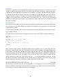
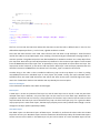
An important part of JavaScripting is creating functions for use later in the code. An example could be this:
function syntaxer(a,call){
var t ='';
for(var i =0; i < a.length; i++){
t = t + call+" = "+ a[i]+" or ";
}
t2 = t.substring(0, t.length -4);
return t2;
};
Here, a function called ‘syntaxer’ is defined. It should have two arguments a list ‘a’, and a string ‘call’, and
t2 which is a string is what is returned. This particular function will concatenate a string with the elements
from the list ‘a’ with the string ‘call’ and some other strings and then return the result string to where the
function was called. The first line within the function is where a local variable ‘t’ is defi ned. ‘t’ can only be
used inside this function, and is not defined in the rest of the script. The for-loop is iterated over the
number of elements in the list ‘a’. The loop will add call, ‘ = ‘, the iterated element of a and ‘ or ‘ to the
string for every iteration. Then the next line will remove the last 4 characters of the string. And finally the
string is returned to where ever the function is called. If the following code is used:
strvar = syntaxer([a,b,c],'type');
Then the variable strvar would contain the string 'type = a or type = b or type = c' . And strvar
could be used in the code. Here the order of appearance is very important. A function cannot be called
before it is defined, and the code is executed from top to bottom, this means the function mu st be defined
prior to the call, and the use of the strvar must be subsequently.
28
Usually you would want JavaScript for dynamic interaction between the website and the user, and example
could be, checkboxes. Checkboxes can be defined in a number of ways; the following code will demonstrate
how to use the result:
//get the type checkboxes
var ct2 = formAdv.getForm().getValues()['checktype2'];
var ct4 = formAdv.getForm().getValues()['checktype4'];
var ct5 = formAdv.getForm().getValues()['checktype5'];
var ct99 = formAdv.getForm().getValues()['checktype99'];
if(ct2 !='on'&& ct4 !='on'&& ct5 !='on'&& ct99 !='on'){
alert('No facility types selected');
}
else{
//array for making string to parse to sql view for the facility types
var a =new Array;
if(ct2=='on'){
a.push('2');
}
if(ct4=='on'){
a.push('4');
}
if(ct5=='on'){
a.push('5');
}
if(ct99=='on'){
a.push('99');
}
types = syntaxer(a,'type');
}
First, four local variables are defined, they are set to either ‘on’ or ‘undefine d’ whether the four checkboxes
are checked, ‘on’ or not ‘undefined’. The checkboxes are elements of the form called ‘formAdv’ and they
are individually called ‘checktype2’...’checktype99’. Then there is an if-, else-statement, checking whether
any of the checkboxes are checked or not. If none are checked, an error message will appear.
If this is not the case, the else-code will be executed. Here an Array (a list) called ‘a’ is created locally. The
list will then have 1-4 elements appended with the JavaScript build in method push. In the end a global
variable will assigned to a string using the function syntaxer, which was explained in the first part of this
section.
Important syntax to notice is the semicolon, in the end of each executed line. If a line is b roken up into
several lines, but only have one semicolon, it will be read as one long line. This is very different from the
python syntax, where line breaks has the effect that semicolons have here. Every executed part of the
code, is embraced in curly brackets {}. // makes the rest of the line, a not executed comment. And indenting
is only for readability, this means that Java Scripts can be minified. If all unnecessary spaces, line breaks and
comments are removed, the code will be shorter and work faster, but will be impossible for people to read.
XML - Extensible Markup Language
XML is a markup language that allows users to define their own tags and attributes. XML is platform
independent as it is a plain text file. Besides, XML is self descriptive where people can easily read and
understand its tags and attributes. XML is well structured so it can be processed automatically. XML is a
29
kind of umbrella language for all kinds of elements like GML. The new versions of HTML use XML. XML
serves different purposes from displaying geographical information to solving mathematical formulas.
Because of these advantages, XML is the most commonly used data exchange format on the Web. On the
other hand, as it uses tags to delimit data it is bulky sometimes. On the other hand, parsing XML is not
efficient especially in languages, such as JavaScript, the most commonly used scripting language on the
Web (Fu and Sun 2011). See next section for an example of XML.
JavaScript Object Notation (JSON)
JSON is a lightweight computer data interchange format which is based on JavaScript Programming
language as defined in the ECMA (European Computer Manufacturers Association). It is easily
understandable. JSON is smaller than XML and it is easy for machines to parse and generate as JSON is a
native data type. Mainly JSON serves as an alternative to the XML format. JSON is completely language
independent but cooperates with C-family languages, including C, C++, C#, Java, JavaScript, Perl and Python
etc. All these properties make JSON an ideal data interchange language (Fu and Sun 2011).
Example of XML and JSON is given below:
An XML example
<?xmlversion= "1.0"encoding ="UTF-8"?>
<students>
<student>
<name>John</name>
<hobby>Basket Ball</hobby>
</student>
<student>
<name>Lisa</name>
<hobby>Movie</hobby>
</student>
</students>
A JSON example
{"students":[
{"name":"John","hobby":"Basket Ball"},
{"name":"Lisa","hobby":"Movie"}
]
}
Python
Python is one of the few programming languages which can be used simply and powerfully with both the
beginners and experts (Swaroop 2005). It is easier to concentrate of problem solution in Python than
making the syntax and structure of other languages.
“Python is an easy to learn, powerful programming language. It has efficient high-level data structures and
a simple but effective approach to object-oriented programming. Python's elegant syntax and dynamic
typing, together with its interpreted nature, make it an ideal language for scripting and rapid application
development in many areas on most platforms” (Swaroop 2005, 1).
Python has several key features. It is a simple language and easily readable. Python is extremely easy to get
started with as it has very simple syntax. Python is a Free/Libre and Open Source Software (FLOSS). It is
30
easily available. It does not require high level of language. Python is object oriented language where it
combines data with functionality. Python programs are easily extensible to the other languages. Python has
a standard library which has modules for every task (Swaroop 2005).
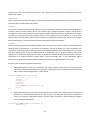
Common language examples
Python scripting can be used for file handling. For this feature it is relevant to import modules. Modules are
language and functionality extensions, that can be imported to extent the features of a python script.
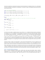
Consider the following code:
infn =r"C:\Users\Thomas\Documents\My Dropbox\Wastewater\data\working
data\dataslimmed.csv"
inFile = open(infn,"r")
This piece of python code will allow the script to read the document, dataslimmed.csv and process the data
it holds. If the dataslimmed.csv is a semicolon separated table, the data can be inserted into a dictionary
like this:
dict ={}
for line in inFile:
aList = line.split(";")
dict[aList[0]]= aList[1:len(aList)]
inFile.close()
Notice the use of the for-loop starting the iteration over each line in the inFile (line 2). This will achieve that
the two indented lines of code will be run for each line in the csv document. The variable line, will change
to be the actual line read from the file.
An important module, specifically for GIS usage, is the ArcPy module import arcpy. This module will
allow ArcGIS functionality inside a python script. For example we would be able to make a database table
like this:
tableName ="table"
arcpy.CreateTable_management(r"C:\path\stations3.gdb", tableName)
arcpy.AddField_management(tableName,"name","STRING")
arcpy.AddField_management(tableName,"column0","INTEGER")
arcpy.AddField_management(tableName,"column1","FLOAT")
This will create a table in the specified file geodatabase of the name ‘table’, with three columns, one string,
one integer and one floating point value.
cur1 = arcpy.InsertCursor(tableName)
for i in dict.keys():
row1 = cur1.newRow()
row1.name = i
row1.column0 = dict[aList[i]][0]
row1.column1 = dict[aList[i]][1]
cur1.insertRow(row1)
del cur1, row1
This piece of code, will copy the dictionary into the database file, usi ng the ArcPy added functionality.
31
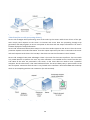
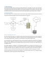
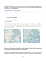
2.5 Web based GIS
WebGIS helps to make geographical information available to the clients. The internet browsers have access
to GIS applications without buying the software while map services allow GIS applications without hosting
them locally having the latest updates. Often client has open access to filtered data. WebGIS is usually
based on server side and client side strategies. In a client / server network arrangement the network
services responds to the requests of clients. The other components of WebGIS consist of GIS database
server, GIS server and the Application server (Figure 11). The GIS database server supports a frequently
access to data and the GIS server supports a large number of users.
Figure 11 The components of WebGIS
Web server mainly sends ready-made map images and applets (JavaScript program). It also passes requests
to CGI programs for further processing. The application server manages connection between web server
and map server. It also interprets requests and passes it to the map server. Application server handles
transaction and security. Map server as a major component of Internet GIS performs spatial queries,
analyses, generates and delivers maps to the client. A web mapping server uses different protocols from
HTTP like Web map service (WMS), web feature service (WFS) and many others protocols to respond the
client. The protocols are designed specifically for the transfer of geographic information, whether it is raw
feature data, geographic attributes, or map images. See Figure 12: A common web based GIS System with
Getcapabilities server for examples of this (Peng and Tsou 2003).
Figure 12: A common web based GIS System with Getcapabilities server (Peng and Tsou 2003, 168)
Open Geospatial Consortium (OGC) Standards
The Open Geospatial Consortium (OGC) consists of 483 companies, government agencies and universities
that have mutual understandings to develop publicly available interface standards. OGC standards support
32
interoperable solution and empower technology developers to make complex spatial information and
services accessible and useful with all kinds of applications. The main purpose of OGC is to serve as a global
forum for the collaboration of developers and users of spatial data products and services, and to advance
the development of international standards for geospatial interoperability. One of the main goals of OGC is
to provide guidelines for internet GIS so it can be communicable with others (OpenGeospatialConsortium
2013). The interoperability program of OGC covers wide range of areas, from geospatial data to geospatial
processing. Web mapping is one of them. The OpenGIS Web Map Service (WMS) interface implementation
specification was published in April 2000 which focuses on how to describe a Web map server and map
services with standardized URI syntaxes and semantics. WMS operations can be done by submitting
requests to the web browser in the form of Uniform Resource Locators (URLs). WMS implementation
interface specification indicates that WMS should be able to do three tasks: produce maps, answer queries
and tells other programs about the map (Peng and Tsou 2003). OGC also provides standards for Web
Feature Service (WFS). WFS not only shares data but it also uses File Transfer Protocol (FTP). It allows
clients to retrieve and modify data. In ISO 19119, the WFS is primarily a feature access service which also
includes elements of a feature type service, a coordinate conversion/transformation service and geographic
format conversion service (OpenGeospatialConsortium 2013).
Web Map Service (WMS)
Web Map Service (WMS) provides HTTP interface to fulfil the request of a client for geographic map
services. WMS provides the interface with geo-registered map images from different databases as JPEG,
PNG or another format. This image is then further viewed in the web browser. The interface also provides
transparent images so that layers from multiple servers can be joined (OGC 2012).
Mainly WMS focuses on describing a web map server and map services with standardized URI syntaxes and
semantics considering three major tasks. It is needed to mention here that a URI is a short string that is
used to identify resources in the web. Therefore, WMS should be able to:



Produce a map (as a picture, as a series of graphical elements or as a packaged set of geographic
feature data)
Answer basic queries about the content of the map
Tell other programs those maps it can produce and which of those can be queried fu rther (Peng
and Tsou 2003, 192).
WMS architecture
Besides the three major tasks of WMS, there are four major processing stages in WMS: filter service,
display element generator, render service and display service. Cuthbert (1997) mentioned about these four
stages which describes data visualization from data to map that is showed in Figure 13:
Stage 1: the selection of geospatial data to be displayed
Stage 2: the generation of display elements from the selected geospatial data
Stage 3: the rendering of display elements into a rendered map and
Stage 4: the display of the rendered map to the user
33
Figure 13: Map display process and relationship with clients (Source: (Peng and Tsou 2003))
The whole map display process can be integrated with the client server relationships for example, thin
client, thick client and medium client. If only rendered map is carried over the Internet to the client, it will
be a thin client system. There is no client side capabilities present in the process. GIF files are such kinds of
rendered maps. If the display elements are carried over the Internet to the web browser, it would be a
medium-client system. Medium client system allows very limited opportunity for client side processing like:
panning, zooming and selection. And if the geospatial data and display element generator service is carried
over the internet to the web client, it would be a thick client system which provides with unlimited
opportunities from client side (Peng and Tsou 2003).
WMS specifications
The WMS specification covers primarily the picture class where only pictures of maps are shown to the web
client while all other tasks including data selection, map rendering are conducted in the server. Map servers
should be able to answer the user’s request. Especially three functions are needed to consider. First, the
map server should be able to provide users with maps in their browser, secondly, provide information
required by the client for example, information on specific areas and specific layers. And finally, the map
server should be able to provide information on map interfaces and map layers that it can serve. These
three functions are supported by three WMS interfaces: map, feature and capabilities interface which are
also known as GetMap, GetFeatureInfo and GetCapabilities (Peng and Tsou 2003).
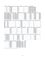
GetMap
Map request interfaces mainly focuses on the display and production of web based map services in the
form of gif, png, tiff. The URI parameters provides the information regarding the coordinate system of the
map, area, information to be shown, output size, format, rendering style and other parameters like map
layers, picture format, picture format, background colour etc. Table 1 shows the parameters used in the
map request interfaces (Peng and Tsou 2003).
34
URL Component
http://server_address/path/script?
WMTVER
REQUEST=map
LAYERS=layer_list
Description
URL prefix of the server
Request version, required
Request name, required
Comma-separated list of one or more map
layers, required
Comma-separated list of one rendering style
per requested layer, required
Spatial reference system (SRS), required
Bounding box corners (lower left, upper right) in
SRS units, required
Width in pixels of map picture, required
Height in pixels of map picture, required
“TRUE”/”FALSE”: If TRUE, then the background
color of the picture is to be made transparent if
the image format supports transparency:
optional: default = FALSE
A hexadecimal red-green-blue color value
(0xrrggbb) for the background color optional;
default = 0xFFFFFF
STYLES=style_list
SRS= srs_identifier
BBOX=xmin,ymin,xmax,ymax
WIDTH= output_width
HEIGHT= output_height
TRANSPARET = true_or_false
BGCOLOR=color_value
Table 1: According to OGC, 2000 Map Request Interfaces (Peng and Tsou 2003, 196)
GetFeature
The feature request interfaces identify the request mechanisms for map contents and feature attributes. It
answers the queries regarding what map layer is being queried and the location of places on the map
showing the coordinates (Peng and Tsou 2003).
Table 2 shows the elements of feature request interfaces
URL Component
http://server_address/path/script?
WMTVER
REQUEST=feature_info (map request copy)
QUERY_LAYERS=layer_list
Description
URL prefix of the server
Request version, required
Request name, required
Comma-separated list of one or more map
layers, required
Return format of feature information, optional
How many features to return information
about, optional
X coordinate in pixels of feature (measured
from upper left corner = 0)
Y coordinate in pixels of feature (measured
from upper left corner = 0)
INFO_FORMAT= output_format
FEATURE_COUNT=number
X=pixel_column
Y=pixel_row
Table 2: According to OGC, 2005 Feature request Interfaces (Peng and Tsou 2003, 197)
GetCapabilities
The capabilities request interfaces is used to provide extensive map services like catalogue services or
metadata queries. For example, to ask a map server about its holdings, the URI parameters can be included
in the capabilities requests, such as “database=Colorado+California” (Peng and Tsou 2003).
35
URL Component
http://server_address/path/script?
WMTVER
REQUEST=capabilities
Description
URL prefix of the server
Request version, required
Request name, required
Table 3: According to OGC, 2005 Capabilities Request Interfaces (Peng and Tsou 2003, 198)
Web Feature Service (WFS)
WFS provide specified geographic features in vector format for user interaction by following OGC standard.
WFS helps clients to perform different kinds of operations including, insert, update, delete and query for
geospatial feature data residing on the server. According to OGC (2005) WFS defines the foll owing main
operations:
Get capabilities: Requests service metadata. The response is an XML that describes service content and
capabilities, including the feature types it can serve and the operations it supports.
DescribeFeatureType: Requests the structure of the feature type that WFS supports.
GetFeature: retrieves a geographic feature and its attributes to match a filter query.
LockFeature: Requests the server to lock on one or more features for the duration of a transaction.
Transaction: Requests the server to create, update and delete geographic features.
(Fu and Sun 2011, 72)
Based on these operations, two main classes of WFS can be defined namely: basic WFS and transactional
WFS (WFS-T). Basic WFS is considered a read only WFS. It implements GetCapabilities, DescribeFeatureType
and GetFeature while WFS-T implements all the capabilities of basic WFS with the transaction operation.
This also implements the Lock Feature operation. WFS-T is considered as a read/write WFS. WFS can be
used for mapping and query. It is also used for geographic data clipping, projection, zipping and shipping
(Fu and Sun 2011).
GeoServer 2.1.3
GeoServer is an open source software server written in JavaScript language, which allows users to view,
edit and share geospatial data by following Open Geospatial Consortium (OGC). It shares data from any
major spatial data sources for example from files on the local disk to databases as it is designed for
interoperability. GeoServer creates maps in different output formats through following Web Map Service
(WMS) and Web Feature Service (WFS) standards. GeoServer operates data through workspaces, stores,
layers and styles. GeoServer also integrates which make map operation (GeoServerA 2012).
36
Figure 14 GeoServer admin page
A workspace groups similar type of data. It is a container that contains similar types of data. If there
presents no name conflicts among the layers then it is possible to use identical layers in different places.
Normally workspaces are presented by a prefix to a layer or store name. Stores, layers, layer groups all
must have an associated workspace (GeoServerA 2012).
Stores contain geographic data in GeoServer. It contains specific data sources that GeoServer supports. Like
databases which contain many tables, stores also contain many layers. Stores must be associated with a
workspace (GeoServerA 2012).
Like stores, a layer must be associated with a workspace. A layer is a collection of geospatial features or a
coverage which is also the smallest grouping of geospatial data. It contains single type of data (points, lines,
polygons, raster etc.) having a single identifiable content (type- e.g. roads, lakes etc.). It corresponds to a
table or view from database. GeoServer stores information which is associated with a layer, such as
projection information, bounding box, associated styles etc. (GeoServerA 2012).
A layer group is a collection of layers, which makes it possible to request multiple layers with a single WMS.
A layer group contains information about the given layers, order, projection, associated styles et c. This
information can be different from the defaults for each individual layer. Each layer group must be
associated with a workspace. Every layer must be associated with at least one style, and GeoServer
recognizes styles in Styled Layer Descriptor (SLD) (GeoServerA 2012).
A style is a visualization directive for rendering geographic data. A style can contain rules for colour, shape,
and size, along with logic including attribute based rules and zoom-level-based rules (GeoServerA 2012).
Parametric view
The parametric view, or the SQL view, is a feature in GeoServer, allowing parameterized queries using
string substitution to a spatial database (GeoServer 2012). WMS or WFS can, as previously described, be
used to represent data from spatial databases. With the parametric view, a dynamic view to the spatial
37
database can be created. This allows for querying using SQL, and in the SQL parameters can be inserted like
this:
SELECT*
FROM
spatial_data
WHERE column_name =%value%
Here %value% is the parameter adding the dynamics to the query. When the WMS or WFS is requested in
JavaScript from the GeoServer, parameters can be set to alter the view.
An example could be:
layer.mergeNewParams({viewparams:'value:100'});
Then only entries in spatial_data where column_name = 100 will be in the view, which will reduce the
number of features in the layer. Even more dynamics can be added to the query if the left part of where
equation is parameterized, or other and bigger parts of the query. An unlimited amount of parameters can
be used in the queries, but they must all have default values to use, if no parameter is parsed with the
mergeNewParams command.
Regular expressions
For hackers wanting to gain access to the database that the view is pointing to or even others on the same
server, parameters should be protected using regular expressions also known as Regex. Regex is a language
for matching strings, in GeoServer parametric view, it can be used to limit the amount of legal inputs, and
thereby preventing unwanted use of and access to the database (GeoServer 2012). Regex syntax is not
straight forward and as is stated in the GeoServer handbook “Regular expressions are a complex topic that
cannot be fully addressed here.” (GeoServer 2012) This also holds true here.
The default regular expression is set to ^[\w\d\s]+$ which will accept \w: Alphanumeric characters plus
"_", \d: digits and \s white space characters. But not characters like “ ‘ “, “=”, Danish letters like æ, ø, å, Æ,
Ø, Å and “.”. If special characters need to be accepted this has to be taken into account. Adding single
characters such as “ ‘ “ can be done by adding \’ to the expression (e.g. ^[\w\d\s\’]+$). Other examples
can be ^[\d\.\+-eE]+$ which only accepts floating point values, which the default does not because
floating point can include the character “.”. And [^;']+ Accepts everything except “ ‘ “ and “;”, which
prevents most hacking attacks (GeoServer 2012).
OpenLayers
OpenLayers is a client-side JavaScript framework which makes it possible to put a dynamic map in most
modern web browsers. Since it is a purely client-side application, it is independent of any server. It is
capable of supporting various mapping APIs such as Google, Yahoo, OGC WMS, OGC WFS, KaMap, Text
layers to name just a few. One big advantage of OpenLayers as compared to its commercial counterparts is
that its JavaScript library is open source making it free for any user. It can be driven easily with any server
language such as PHP, PERL since it is a pure client-side application. Maps can also be embedded directly
into a plain HTML file in order to build one’s own map as required. Basically, OpenLayers API has two
concepts which are imperative to understand. These concepts are ‘Map’, and ‘Layer’. Even though
OpenLayers is JavaScript based, it does not require one to be an expert in JavaScript language before using
it even though knowledge of it will be very helpful in handling errors in the script (OpenLayers 2012).
38
OpenLayers lives on the client side. One of the primary tasks the client performs is to get map images from
a map server. The client ask the map server for the map in the Bounding Box of the application – every time
a pan/zoom command is issued, the client makes a new request. OpenLayers makes it easy to put a
dynamic map in any web page. It can display map tiles and markers loaded from any source. OpenLayers
has been developed to further the use of geographic information of all kinds. OpenLayers is completely
free, Open Source JavaScript, released under a BSD style License. So, it can be said that OpenLayers is an
Open Source map viewing framework written in JavaScript, an alternative to commercial mapping APIs
which are designed to integrate well with existing GIS. Since OpenLayers uses JavaScript syntax for coding,
the knowledge of code construction from the previous course is required (OpenLayers 2012).
An OpenLayers Map stores information about the default projection, extents, units, and so on of the map.
Data is displayed within map via Layer and a Layer is just an information source for data about how
OpenLayers should request data and display it. In order to build OpenLayers viewer, we need to craft HTML
to be seen by the viewer and a map can be put inside any block level element. This means that we can put a
map in almost any HTML element on a page. One is required to include a script tag pointing to the
OpenLayers library to a single level element (OpenLayers 2012).
It is not always necessary for the location of the library to point to the .js file on the OpenLayers server. We
can download the full code and run it locally by using the script
src="..." equal to the location of the library on the local hard drive (OpenLayers 2012).
Creating maps with the OpenLayers
The following steps are needed to create a web application:
1. Link to the OpenLayers library files
2. Create a HTML file that will hold the script
3. Create a map object
4. Create a layer object
5. Add the layer to the map
6. Define the maps extent
The basics Code
<!DOCTYPE html>
<htmllang='en'>
<head>
<metacharset='utf-8'/>
<title>My Map</title>
<scripttype='text/javascript'src='-2.11/.js'></script>
<scripttype='text/javascript'>
var map;
function init(){
map =new .Map('map_element',{});
var wms_layer_map =new .Layer.WMS(
'WMS Layer Title',
'http://vmap0.tiles.osgeo.org/wms/vmap0',
39
{layers:'basic'},
{}
);
map.addLayers(wms);
if(!map.getCenter()){
map.setCenter(new .LonLat(10,55),6);
}
}
</script>
</head>
<bodyonload='init();'>
<divid='map_element'style='width: 500px; height: 500px;'>
</div>
</body>
</html>
The first 1-7 lines are the basic html where the character set and the title is defined. Here in line 6 it also
defined the OpenLayers library. And in line 9, a global variable is created.
There are two main sections in the code. One is function init and other is map add layers. These functions
load all the code to set up OpenLayers map. Creating a function that gets called when the page loads is a
common practice. The global map which was declared before is needed to make it into a map object from
the .map class. Here the map class ID (map element) is defined. In this section a layer object is also created
from the WMS subclass of the Layer class. In OpenLayers, every map needs to have at least one layer. The
layer points to the 'back end', or the server side map server. Here layer`s title and layer properties are also
declared. The source of WMS file is also shown here. Thus wms_layer is created in this section.
Another thing in the code is that it needed to add wms_layer to the map object. It is done by calling
map.addLayers where an individual layer or many layers are passed. Finally, the map's viewable area is
specified. Here, the actual code that moves the map to the zoom centre point. The final digit is the zoomlevel. This if-statement checks to see whether the map already has a centre point.
Basic terminologies
In this subsection we define some basic terminologies.
Base Layers
A base layer is at the very bottom of the layer list, and all other layers are on top of it. One may also have
multiple base layers. However, only one base layer can be active at a time. Base layer determines the
projection and zoom level on the map. The projections of the other layers need to be the same as base
layer otherwise the base layer can be distorted. Any layer can be a base layer only if it is given the Base
layer property but in most raster layers, the Base layer property set to true by default even though it can be
changed in the layer options (OpenLayers 2012).
Non Base Layers
Non Base Layers are alternative layers of Base Layers. Therefore it performs the other tasks which Base
Layers do not carry out. Non Base Layers are also sometimes called Overlays. Many of the Non Base Layers
can be active at a time while in the Base Layer only one can be active at a time. Non Base Layers do not
40
support the zoom control while some layers can support re-projection to the base layer projection
(OpenLayers 2012).
Raster Layers
Raster Layers are composed with pixels. These are fixed with the projection and cannot be changed from
the client side view side (OpenLayers 2012).
Overlays
All the layers except the base layer are called overlays. In OpenLayers there are Vector Overlays and Marker
Overlays. Vector overlays present data in the browser. Lines, polygons and other features can be drawn
through the vector overlays. Marker overlays display HTML image objects. More capabilities for example,
maintenance, interaction with the remote severs can be earned from vector overlays as it gives more
opportunities to present data. Marker layers supports the capabilities which vector layer cannot support.
Mainly Marker layer is maintained for backwards compatibility (OpenLayers 2012).
GeoExt
GeoExt combines geospatial knowledge of OpenLayers with the user interface of Ext JS to build powerful
desktop style GIS applications on the web with JavaScript. The aim of GeoExt is to make a powerful and
resourceful presentation style of GIS applications on the website with the help of JavaScript. It is also client
side web mapping with an open source extension to OpenLayers. It can support toolbars, map panel,
legends, print, zoom level, layer selection, scale etc. GeoExt is used here to integrate ext interfaces with the
OpenLayers as it makes possible to handle data in more presentable way. In the OpenLayers legend
functions are not directly available therefore, GeoExt is used to build legend modules in the map.
Here are some examples of geoext elements are:

MapPanel element is the most important and used in GeoExt applications. Using OpenLayers
JavaScript, it displays rendered data using popular mapping services as Google Maps or Open Street
Map. A Map Panel coding example is shown below.
mapPanel =new GeoExt.MapPanel({
title:"GeoExt MapPanel",
region:"center",
height:400,
width:600,
map: map,
center:new .LonLat(146.4,41.6),
zoom:7
});

LegendPanel element is a panel that shows legends from all the layers in the layer store. The legend
elements are displayed depending on the type of layer. The displayed data can be configured in
layer store using the configuration options: dynamic, filter, layerstore or preferredTypes. A Legend
Panel coding example follows.
legendPanel =new GeoExt.LegendPanel ({
defaults:{
41
labelcls:"mylabel",
style:"padding:5px",
width:350,
autoScroll:true,
region:"west",
});

Ext.Panel element defines the interface of the GeoExt application arranging and putting together all
the panels declared and included into Ext Panel. An example of Ext Panel is shown below.
new Ext.Panel({
title:"GeoExt LegendPanel Demo",
layout:"border",
renderTo:"view",
height:400,
width:800,
tbar:new Ext.Toolbar({
items:[
{text:"add/remove", handler: addRemoveLayer},
{text:"movetop/bottom", handler: moveLayer},
{text:"togglevis", handler: toggleVisibility},
{text:"hide/show", handler: updateHideInLegend},
{text:"legendur1", handler: updateLegendUr1},
]
}),
items:[ legendPanel, mapPanel]
});
Styling the WMS
Styled Layer Descriptor (SLD) extends the WMS standard to allow user defined symbolization and colouring
of geographic features (Open Geospatial Consortium 2012). SLD is an OGC styling language standard that
both the client and server can understand. It includes a StyledLayerDescriptor XML element that contains a
sequence of styled-layer definitions (Open Geospatial Consortium Inc. 2007). Here is a simple example of a
SLD that defines the style of a point:
<NamedLayer>
<Name>Default Point</Name>
<UserStyle>
<Title>Point feature</Title>
<Abstract>This style styles a point feature with red squares</Abstract>
<FeatureTypeStyle>
<Rule>
<Name>Rule 1</Name>
<Title>RedSquare</Title>
<Abstract>A red fill of squares with a pixel size on6</Abstract>
<PointSymbolizer>
<Graphic>
<Mark>
<WellKnownName>square</WellKnownName>
<Fill>
<CssParameter name="fill">#FF0000</CssParameter>
</Fill>
</Mark>
<Size>6</Size>
</Graphic>
42
</PointSymbolizer>
</Rule>
</FeatureTypeStyle>
</UserStyle>
</NamedLayer>
</StyledLayerDescriptor>
This example is simple with the following elements: Name, Title, Abstract and a Graphic with one defined
colour, size and shape. More advanced styling available as well. More colours can be defined corresponding
to attributes or corresponding to a certain zoom level. SLD can be divided in rules and each rule can have a
filter generated in the attributes. This filter describes which records to render. Multiple symbolizers
describe how those records are rendered (Open Geospatial Consortium Inc. 2007).
Many examples are found through the SLD Cook Book (Pumphrey 2012). But the frame of the possibilities
of SLD is much more widespread than the content of this book. The legend is created through the SLD as
well. Each time there is a call to the WMS; the legend is refreshed and shows all graphic styles that are
shown in the certain session (Open Geospatial Consortium Inc. 2007).
2.6 Cartography theory
Information on a map is a representation of the real world. It is an attempt to reproduce information on a
way that makes the information understandable for the “consumer”. To make information understandable
is an infinite discussion on what understandable is. Traffic lights show information on when to go and when
not to go with the colours of red and green. The problem with this is that one in every 10 persons are
colour-blind on red and/or green (Brodersen 2008). With this in mind it would be obvious to use other
colours. But what colours can be understood by the majority as go and not go instead of green and red?
To manage all the possibilities there are available within the visualization of information representation on
a map, Brodersen (2008) made a model to run through during the developing progress of the design of the
map. In Figure 15 the model is presented. The model contains five basic elements:





Values are about the values that justifies the project. Who is the producer and what will he use the
project for?
Content is the content that enables that the user can solve his tasks.
Apparatus is the part that the user, through the use, gets in contact with the content.
Interaction is about how the user through the apparatus gets in contact with the content.
Expressed information is what the user sees.
43
Figure 15 Geo-communication and informati on design model (BrodersenA 2008)
Brodersen (2008)distinguish between four tools within the expressed information. The laws of gestalt are a
main tool. It is about how a visual impression is perceived. An example could be a consideration about how
we would know that a green polygon necessarily means a forest on a map. In a visual hierarchy it is
determined which elements are visually dominating (and important). Brodersen (2008) tells for instance
that warm, intense and sharp colours symbolize the point in the map, while they seem strongest. The level
of abstraction is a matter of preferences among the users. It is of course vital to understand the user’s
ability to learn about these abstractions. The graphical variables can consist of points, lines, polygons,
pictograms, text etc. These can vary in size, darkness, shape, colour, orientation, texture etc. In general will
no visualization ever be perfect, but with a little consideration, the level of satisfaction a person gets using
a product will increase (Fu and Sun 2011).
Representation of geographic data
The spatial information is distinguished by other kind of information through an important element, the
geographic location. Representing data in GIS systems is related to representation of geographical location.
The biggest benefit of GIS is the location because different kind
of information can be visualized in the same geographic
location. In GIS if there is more information that has the same
location it is fundamentally to have the layers that the data is
represented on, aligned. If the layers are not aligned then a
common spatial reference system must be chosen. (Longley
2004)
The spatial reference system is defined by projection,
coordinate system and datum. The features usually have their
location represented on the surface of earth based on
geographic coordinates while most GIS data is visualized on a
plane map. In this case the map features are based on x and y Figure 16 Measurements of geographic
coordinates while the objects have geographic coordinate coordinates (Kunen, 2008)
system which is usually represented in longitude and latitude. Here the map projections become very
44
important in building a link between the two types of coordination systems. The principle of projection is to
transform spherical surface into plane through mathematical expressions. Most of the GIS projects use data
from different sources that do not have the same coordination system so they have to be projecte d or reprojected before using. (Longley 2004)
Geographic Coordinate Systems
The location is defined on Earth`s surface by latitude and longitude. The representation of geographic
coordinates is made with respect to Greenwich and The Royal Observatory. The geographic coordinates’
notation is such as the plane coordinates with longitude as x and latitude as y. the coordinates can be
either positive or negative depending on the reference lines. The longitude values that are measured in the
eastern hemisphere are positive and negative in western. It is the same with latitude; the values are
positive in the north and negative in south. (Longley 2004)
When mapping spatial features a model that approximates the surface of Earth is needed. The sphere is the
simplest model that the Earth can be represented on, but this planet is not perfectly circular so a better
approximation is a spheroid or an ellipsoid. (Longley 2004)
The datum is used to create a reference for the geographic coordinates and it consists of an origin and the
parameters of the selected ellipsoid. There are various coordinating systems and most of the countries
have created their own for an easier measuring inside their borders. Some examples of coordinating
systems are: WGS84 (World Geodetic System), NAD83, GRS80 etc. (Longley 2004)
Projected coordinate systems
The projected coordinating systems are map projections of converted geographic coordinates to plane
coordinates. This is done using mathematical expressions. The projected coordinating systems have a
constant area of length and angle across 2 dimensions contrast to the geographic coordinate system. The
most common map projections are Transverse Mercator, Equidistant Conic, Albers Equal -Area Conic and
Lambert Conformal Conic. The most used systems are The Universal Transverse Mercator (UTM) Grid
System, the State Plane Coordinate System (SPC) and The Universal Polar Stereographic (UPS) Grid System.
A very important aspect is that changing the coordinates for a location is related to the datum and ellipsoid
under which the coordinates were based. (Longley 2004) (W. Paul 2004)
It is a must to realize and understand for GIS applications that each UTM zone has a different projection
and system of coordinates. When a bigger area is shown and maps from different UTM zones are merged
into a single map, some distortions may occur. This problem can be overcome by using a different
coordinating system and re-projecting the data. (Longley 2004)
EPSG Geodetic Parameter Dataset
Workings with GIS involve a lot of coordinate transformation. That means that a data registry about
coordinates reference systems and transformations is required. “The EPSG Geodetic Parameter Dataset is a
structured dataset of Coordinate Reference Systems and Coordinate Transformations, accessible through a
data registry.” This registry has geographic data coverage of the whole world but unfortunately it cannot
cover all possible geodetic parameters used around the world. The Geodetic Parameter Dataset is
maintained by a subcommittee of International Association of Oil and Gas Producers (OGP). (Registry, 2013)
45
The projections are defined in GeoServer in ESPG codes. If the data that has to be published in the
GeoServer do not have an equivalent projection in ESPG code, then a custom ESPG code can be created.
The data used in this project has a well-defined ESPG code so it is irrelevant to discuss how to create a
custom code.
46
3. Methodology
In this part the process used for achieving the desired objectives is described. First there is the description
of the system design documented and argued. Further on is the implementation chapter where the system
is detailed and the reasons why there were chosen specific procedures are presented. The chapter ends
with data description and preparation where data is described in details and the preparation are argued.
3.1 System design
The system design is the conceptual implementation of the project. Based on the tools that were used the
project has the following diagram that is described and shown in Figure 17:
Figure 17: System design of the project
The main idea of the project is to display and work with the geo-referenced data on a map through the
web, in this case represented on a website. In order to do this, a spatial database had to be created from
the initial data “WinSpv data” received in an excel document using python programming.
The input data for the spatial database has three entries because, besides the starting data (the WinSpv)
there has been designed an upload data python script that converts the data into executable SQL
commands and sends them to the database and one more entrance is the over layer “Municipality” is
uploaded manually.
The Spatial Database is mediated on the PostGreSQL program that is linked to the Geo Server on two
directions. The first link is directly to the GeoServer because it is using the data from the Spatial Database
through PostGreSQL the server requests to SQL program on parameters used on the website through the
parametric view is the second. These processes are done automatically when the webpage is accessed.
Finally using JavaScript all the parts are put together in the html document and run as a website through
the GeoServer and with the service from Open Street Map.
47
Web architecture
As the system design shown in Figure 17: System design of the project suggests, most of the work is done
on the server side. The layers are communication between GeoServer and the databases, which is hosted
by a server. The background map, is also hosted from a server, this is just externally (cloud based). But the
system is still a hybrid, because a few layers are operated on the client side. These are WFS -layers used for
the operation of controls, and GeocoderComboBox. These WFS-layers are very lightweight and will not be
saved anywhere outside the application. Therefore the application can be described as a client -server
hybrid strategy, albeit much closer to a thin-client than a thick-client.
Database structure design
In the following the design of the databases serving the WinSpv data will be described. As previously
described, a sensible database design is essential for speed and flexibility. For this purpose a relational
database is chosen for the database design.
In the original WinSpv table, there were a lot of abundances and not all the needed data. So a
normalization process and a database design were obvious choices. The WinSpv holds both data about the
measurements and the facilities, so an obvious start is to split this up and create ids as primary keys. To see
an example of the WinSpv table, see the section “Preparation”.
Figure 18 First step in normalization of the databases
The first step as depicted in Figure 18 achieved to get rid of all abundances related to facility data which
initially were there for each measurement. In order to get the needed information about the measured
compounds and limits, this data needed to be added to the database in order to not interfere with the
normalization of the database, therefore database describing compounds was related one -to-one with the
compounds (one compound measured in one measurement). The limit values are specific to both the
facilities and to the compounds. Therefore a fourth database with a one-to-many relationship the facilities
(one facility has many limits) and a one-to-many relationship to the compounds (every compound has limits
for each facility) was added.
48
Figure19 - ER-diagram
Facilities are uniquely identified by a Facility ID, Measurements by a measurement ID, and compounds by a
Compound ID and limits by a combination of a Facility ID and a Compound ID.
User requirements
To identify our users we have created 3 user types. The types are made from thoughts on who might have
interest to use our system based on information from Danmarks Miljøportal about the users:
User 1: I am working at the Danish society for nature conservation. In my daily work I keep an eye with the
quality of the water in Denmark. It can provoke a catastrophe if wastewater that exceeds the limit values
enters the nature. Easy access to the data is therefore a huge advance in my work to monitor wastewater.
User 2: I am working at the Danish Nature Agency. My organisation has the governmental responsible to
secure that wastewater is not destroying our environment. A better access to data is therefore expedient in
my daily life.
User 3: I am an ordinary citizen and live by the sea right next to a point of discharge from a wastewater
facility. This is normally not a problem due to the good quality of cleaning at the wastewater facility.
However, before taking a swim I would like to be able to see the measurements of each compound.
Therefore I have a huge interest to be able to see data about the point of discharge.
Concluding on the three users we have two main user groups; the professionals and the citizens. In a
professional matter access to the data is quiet political and seems necessary. However, the system is made
public for all so a benefit to publish it is that citizens can get information about the water that they use for
recreational activities.
It is expected that each user group has different preferences to the way to interact with the system. This is
mainly caused by their existing knowledge on the Wastewater-field. A citizen is expected to have a curious
way of acting in the application; while the professionals are considered to do searches depending on their
aim.
3.2 Implementation
The implementation part is where all comes together. The theory is implemented through methodology
using the data. The project idea is to create a WebGIS application and is described in the following steps.
49


System implementation
User interface design
System implementation (Agile implementation process)
When the project work started, the main approach of the work was that which approach it will follow. In
the theory section two strategies are described. Both of the two strategies have pros and cons. Based on
these strengths and weaknesses, the approach of the project is deci ded.
Waterfall approach can be applied if one is aware of the whole process. It has some advantages. It is very
simple to implement. The strategy is a linear model and well documented. In this approach all the things
are needed to document when each step is completed. The biggest problem of this approach is that each
step must be finished 100% before proceeding to the next one. If one fails in one step then it is impossible
to proceed and needed to redo the process. Another disadvantage is that if clients require any changes it is
harder to implement.
On the other hand the agile approach can be applied, even if one is not aware of the whole process and
does not have much experience in developing phase. The work consists of small work cycles or modules. It
is an iterative process. So, it is possible to get a more suitable output for satisfying the product by following
some cycles. The approach relies more on codes rather than documentation. So, there is a very little scope
for documentation. Another problem of the approach is that, it leads higher expectations to get best
possible solution.
We have decided to follow the agile approach as we are dealing this kind of problems for the first time. The
reason behind is that there was no knowledge about the whole process to follow. Again we do not have
experience with fulfilling the demands of waterfall methods. But we have decided to follow the
documentation of the programming and development from waterfall method as the documentation is
necessary for the project.
It was decided to follow agile approach considering all the pros and cons of the two methods as it gives
opportunity to change when it is necessary. If we are getting stuck in one step it is possible to start a new
iteration that does not take much time. The approach provides opportunity to divide the tasks among the
members dynamically so no one had to wait while the others were working. See Figure 20.
50
Figure 20 Agile implementation process
The method is also used because of the short time assigned to this project. In this matter the whole project
was developed in iterations. In the first iteration a simple application with minimum functions was
developed. The database in .xls was transformed in .dbf so it could be imported in pgAdmin. Afterwards the
GeoServer was set up and the html webpage application was developed. Finally the system was tested.
In the second iteration the system was developed. More GeoEXT components were added. The database
limits were set through the parametric view and a compound update script was done. The update button
was set. This is important because all the components from the advanced search are taking effect because
of it.
The third iteration was for improvements. If there is update button, there should be something for the
system to get back to the default values, so a reset button was added. New layers were added and using
the Geocoder two new types of search was set up: the municipalities and facility search.
Web Application Implementation
In the following the implementation of the web application will be described. The implementation of the
web application, in the following, is divided in to three parts; cartography, describing the cartographical
choices and implementation methodology, HTML implementation, describing the structuring of the HTML
document and basic code elements, and the JavaScript implementation, describing the functionality of the
web application.
OpenStreetMap (OSM)
OpenStreetMap provides free geographic data like street maps and encourages the growth, development
and distribution of geospatial data for using and sharing by everyone. It is supported by the
OpenStreetMap Foundation, an international nonprofit organization (OpenStreetMap 2013). The
OpenStreetMap Foundation has some objectives:

To make OSM data available for anyone (for editing and in whole).
51






The data being current.
The data to approach geographic truth (or “ground truth”).
That human add and curate data.
That the data and responsibility for it belong to all contributors.
To facilitate decision-making in the community where necessary.
To be the ultimate “court” of conflict resolution. (OpenStreetMap 2013)
Anyone can download and use map data from OpenStreetMap. But geodata is controlled by a license. The
most positive thing is that it is free to use that means people do not need to pay to use geodata. There is no
copyright, license, usage and other kinds of fees. Anyone can use data for any purposes like personal,
community, educational, commercial, government or any other uses (OpenStreetMap 2013).
Cartography
The user interface is designed with simplicity and intuitiveness in mind. All tools and controls are aimed to
be self explaining in order to maximize convenience of use.
The graphical interface regarding the map and the representation of data is designed to be as simple as
possible at the first look. One thing that can really disturb a map is its background map. We ended up using
OpenStreetMap despite of disturbing symbology. The disturbance consisted of a too detailed symbology
relative to the needs in the system. An example of the symbology is shown in Figure 21. Related to the
theory we know that a map should not contain more information than necessary for the purpose of the
map. Later in the report we will make a perspective on how this can be improved.
Figure 21 Local symbology visually interferes with the point of discharge
Our data is presented through a web map service. The choices for styling in this web map service follow the
model presented by Brodersen (2008) figure 15.
52
The value is that the producer wants to make data more accessible. The way to do this is through the
apparatus called a WebGIS solution. The content is the data from the WinSpv database and the interaction
is how we manage to express the information. We do this through the styling of the WMS as explained
earlier, but how should data be represented visually?
Points will be used to represent each facility and each point of discharge. Since we are showing facilities
that have an exceeded compound value due to the limit at the points of discharge, only points of discharge
will be shown in the first place. Each point will have a red, yellow or green colour depending of the degree
of exceeding the limit value. Green means that limit is not exceeded. Yellow means that the limit is close to
being exceeded and red means that the limit for the certain compound is exceeded. It is defined in the
styling that this will be shown in the range from 1:15.000.000 to 1:500.000. In the range of 1:500.000 the
styling change so it has the name of the facility attached to the point together with the earlier defined
colour.
The pipe between the facility and the point of discharge can be activated by the use. The width of the pipe
on the map is slightly thinner than the point of discharge and the wastewater facility. This is done to avoid
that the pipe seems more important.
The wastewater facilities (treatment sites, as opposed to points of discharge) can as well as the pipes be
activated. The size is the same as the size of the points of discharge. However, the colour of the facilities is
different from any of the discharge points to avoid confusion.
By using different visibility at different zoom levels we make sure that the user does not drown in
information that is not viewable anyway. If we had added all information at any zoom level, it would have
been confusing with too much information.
HTML implementation
The web application is a HTML document. The document consists of two parts; the HTML and the
JavaScript inside the HTML <Script> tags.
The application is almost exclusively running on JavaScript functionality, so the HTML part of the
application implementation is basically just loading files for use in the JavaScript. These are:



Ext JavaScripts and css. Ext is extra JavaScript functionality linked to graphics files (css). So when
new Ext.form.ComboBox is used in the JavaScript, it is known, because it is linked to additional
scripting and graphics in the loaded links in the top
GeoExt.js is a further extension of the possible functionality. This enables the use of a legend panel ,
map panel, feature reader and more
.js is also an extension of the JavaScript functionality. This enables the use of the map, the layers,
the communication with GeoServer
Other than this the title and the character set are assigned.
JavaScript implementation
In the following section, the implementation of the web application using JavaScript will be discussed. The
overall structure will be outlined, and parts of the code will be explained.
53
The JavaScript used in the HTML document can be viewed in full length in Appendix 8.1 “HTML and
JavaScript”. It consists of two main parts:


Initialization, definition and assignment of global variables and functions
functionality, here everything to do with the actual map and layers functionality is executed
Initialization
In the first part of the JavaScript, global variables are defined and assigned default values. This is done in
order for them to be dynamic part of code later on. Their values will change according to the user input,
and will be put to use, in functions and methods.
In the initialization four functions are defined:



syntaxer(a,call) and syntaxer2(a,call). These are used, for making chosen elements
appear in SQL compatible syntax, the code is also explained in 2.4 “JavaScript”.
startpos(). A function that will zoom the map to the extent of all of Denmark.
UpdateView(). This function contains some of the main functionality of the JavaScript. It is run
every time the data from the database should be re fetched according to the user inputs. The most
important part of the code is the layer method layer.mergeNewParams. This makes a request to
the GeoServer WMS with new parameter input for the parametric view. When data is retrieved
from GeoServer, the layer and the legend are redrawn.
When defined, these four functions can be used in the rest of the code. The syntaxer functions are actually
used, in order to call the UpdateView()with SQL syntax for the new parameters.
Functionality
The functionality is implemented object wise. This means that all the visual elements are coded separately
and then put together. The whole page is filled by a viewport. A viewport is a container element from Ext
that can contain other elements, namely the map and panel, so that they will resize to match the page
document. The viewport is defined in the last part of the script. This is because, the elements that is inside
the viewport, must be defined before the viewport, in order for the execution of the code to work
(elements must be defined before mentioned in the code). Inside the vi ewport the following structure
applies:
Viewport

The map. map element
o Background map
o Overlay Layers
 Points of discharge
 Facilities
 Pipes
 Municipality
 Selection layer
o Controls
 Zoombar
54


 Navigation
 getFeature
 Mouse position
Panel in the bottom. Here information about a clicked facility is shown
o Info about clicked features
o Bottom bar
 GeocoderComboBox for facilities
 GeocoderComboBox for municipalities
Panel on the right hand side. Here everything is controlled
o Simple tab
 Legend
 Compounds picker dropdown
 Zoom to Denmark
 Layers add
 Compound information
o Advanced tab
 Custom limits
 Selection of facility types
 Selection of facility ownership
 History slider
 Update button
 Reset button
It applies that every element that is a child of another must be defined before its parent, within its parent
or be added to the parent after both the child and the parent are defined. For example the compounds
picker dropdown is defined before the Simple tab, because it is a child of the Simple tab.
GIS Analysis
In this section we will describe how we have used GIS analysis to create spatial analysis. To create some of
the extra features we added to the application, we used GIS as a tool to create these features. We used
common tools in ArcMap to do the analysis.
GeocoderComboBox data preparation
The GeocoderComboBox.js has a build in configuration of the wanted zoom level. But there is a bug in the
script so it always zooms to the bounding box of the selected feature, ignoring the zoom configuration.
That means if the selected feature is a point, which by definition has no
size, it will zoom as close as the background map allows. This is not desired,
as it is simply too close. The other GeocoderComboBox, used to zoom to
the municipalities had another problem. While the bounding boxes worked
as they should the problem is, that the shape layer of the 98 Danish
municipalities contained 1777 features, of which one could be zoomed to at
a time. This was due to the fact that islands are separate shapes, even
though they are part of the same municipality. Another issue, was that
some of the facilities’ points of discharge, was located in the ocean, outside
55
Figure 22 Example of a buffer
around the facility
the municipality boundaries, and if a municipality was zoomed to, the zoom might now show all the
important features.
To respond to the first issue, 3 km buffer zones around each point of discharge were created. The buffer
size of 3 km was chosen to ensure that when zooming to a facility both the facility, the point of discharge
and the immediate surroundings could be seen. Using the GeocoderComboBox with the buffer zone layer
instead of the point features, will zoom to the periphery and use these as bounding box. See figure 22.
The buffer analysis was done using the Buffer analysis tool in ArcMap. This requires shape file as input and
the chosen buffer size.
The other issue took a little more work to get around. ArcMap has a tool called Minimum Bounding
Geometry, this was applied to both the combined features of
each municipality and the facilities of each municipality, and
then these two were merged and dissolved in one layer, with
98 features named after each municipality.
Figure 23 Minimum bounding geometry for municipality borders and points
of discharge
Figure 24 Result of minimum bounding
geometry for Danish municipalities excluding
Bornholm
The shape setting used is called convex hull, which makes a
polygon, like in Figure 23. In Figure 24, the whole analysis is displayed. When a municipality is chosen in the
GeocoderComboBox, the convex hull, shape will be zoomed to, ensuring all municipality features and
points of discharge will be in the picture.
XY to line
The wastewater reaches the wastewater facility, and is cleaned. From the facility the water continues
through pipes to the point of discharge. We have both the facilities and the points of discharge, but we
need to create our own fictional pipes to visualize that there is a connection between the facilities and the
points of discharge, so that the user knows which facility connects to which point of discharge. This is done
by the XY to line tool in ArcMap. We simply use the two corresponding points to create a straight line that
will represent the pipe.
3.3 Data
How data is structured is a deciding factor for how the work process comes along, and in this chapte r the
relationship between the data and the project will be described. The chapter will focus on data handling as
56
scientific documentation for the purpose of being able to follow the thought processes going on behind the
handling of the data. We will describe how we process the data on its way to be published.
Preparation
To make the data ready for publishing and improve performance some preparation is needed. Data is by
default in .csv format. Table 4 is showing how the first 7 rows of the original data look.
57
Table 4 The first seven rows of the original data
58
Drop null values and other odd values
At first glance some gaps in the data can be found. The gaps are represented by the values; “NULL” or just “
”. Some fields are critical and some are not. It is therefore necessary to decide which fields are critical, and
then filter out bad records. Python scripting is used to do this by reading each line and testing whether they
meet the requirements.
Table 5 Choices concerning use of original data. Critical is data that must not be missing, keep is data kept disregarding quality
and loose is data not used
It is obvious from table 5, that a lot more information could be extracted from the data and possibly put to
good use. This topic is discussed in the 7 Perspectives.
Another important selection, were of the compounds. There was a total of 196 different compounds
measured ranging from Total-N measured 9634 times to several compounds only measured one time. To
limit the number of compounds, only compounds with Danish legal limit values (Miljøministeriet 2011) and
compounds measured at Horsens Centralanlæg (Horsens Vand A/S 2011) were chosen.
Having done these filters the data ended up having around 44.000 records left – corresponding to about 75
% of the data.
Limit values
In order to have a meaningful display of the data, an option is to relate measured values to limit values, this
way it can be shown whether the limits are exceeded or not on the map. Some limit values are national and
some limit values are local and specific to facilities. Data on local limit values are not imme diately available,
so a table was created with the national limits for the compounds where national limits were available and
the rest was filled out with the limits of Horsens Centralanlæg. This means that the visual result for most of
the measured compounds is not corresponding to real value – limit relationship but a pseudo value used
for having some limit data to work with.
Splitting data
Data is now slimmed and ready for implementation. In accordance with our database structure the data is
split into two databases, the Facility database and the Measurement database. Each record is assigned a
unique ID attached. While one facility has many measurements, each measurement gets its corresponding
facility ID attached as well.
59
The split is made using Python scripting. The input file is the output file from the previous processed .CSV
file. We start by defining the table names. We use the function CreateTable_management which is a part of
the ArcPy module. The demanded function parameter is a workspace and the table name. This creates an
empty ArcGIS table. By using the function Addfield_management we create field in the empty table. The
necessary parameters are the table name, the fieldname and the data type.
tableName ="Facilities"
arcpy.CreateTable_management(r"C:\Skole\7 sem\data.gdb", tableName)
arcpy.AddField_management(tableName,"f_id","INTEGER")
arcpy.AddField_management(tableName,"name","STRING")
arcpy.AddField_management(tableName,"muni_code","INTEGER")
arcpy.AddField_management(tableName,"inx","FLOAT")
arcpy.AddField_management(tableName,"iny","FLOAT")
arcpy.AddField_management(tableName,"outx","FLOAT")
arcpy.AddField_management(tableName,"outy","FLOAT")
arcpy.AddField_management(tableName,"type","INTEGER")
(This is an excerpt; there are more actual fields in the table. See Appendix 8.2 “Split data”)
When the fields for the two tables are created we insert a curser in each table. We start reading the data
file in a “for”-loop for each line like described earlier in Common language examples.
There are some lat/lon values which contain a “,” instead of “.”. In order for them to be floating point
values this must be corrected. This is done by using the module re, which has substitution functionality:
if","in aList[10]:
aList[10]= re.sub(',','.', aList[10])
We start writing to each field and define which attributes from the old table goes to which attributes in the
new tables.
Converting from CSV to DBF
In the previous section we showed how to split a .csv file. At the same time we convert it into a database
format that can be handled within databases. The conversion is done by using the
arcpy.CreateTable_management. This creates a new table in a specific workspace.
We use a specific script to convert a couple of tables that are within the .csv format. The script can of
course be modified to delete or replace certain records etc.
Database processing
This section will explain the database querying, done in order to get the relevant data out of the database,
structured as illustrated in figure 25.
The querying is divided in two parts:


Creating a suitable table with all the relevant data, lined up in a way so data can be accessed easily
from this one table. See appendix 8.3 “Creating a table from the databases”.
Creating a flexible view from the table, allowing parameters to control the visual output of the
table. See appendix 8.3 “Parametric view”.
60
A suitable table
Because of the implementation structure we have chosen, one layer in the final webGIS applicatio n is one
database view. For this reason we need to assemble all the relevant data from our four databases in one
table. See ER-diagram figure 16 in 3.1“Database structure design”. The elements required to be in this table
are:




Facility data. This is the address, contact information, facility name, ownership, municipality etc.
Measurement data. We need two columns for each compound, one with the measured value and
one with the corresponding time.
Limit data. Data showing the limit specific to the facility and the compound.
Historical data. In order to show historical data, each historical iteration of the table must be added
to the total table, so that each facility is represented the amount of historical records plus the most
recent data.
Figure 25 Desired look of the final table
The way this is achieved is by splitting the data up in several ways and then combining it again like shown in
Figure 25. In the process more than 100 views are created with exerts of data f rom the measurement
database. The number of facilities is called n and the number of compounds is called m. The following steps
are done to get a suitable result:
1.
2.
3.
4.
5.
6.
7.
7.1
Data must be split on the compounds, so that there is one view per compound.
Data not relevant to the historical datetime must be removed. This results in m*n records.
The two above must be joined in one view per compound. This results in views with n records.
The views from step 3 must be joined together in a ‘full join’ also adding the facility database. This
allows the structure where the compounds appear as different columns for the same facility. This
results a view with n records.
The view from step 4 is then joined together with the limits table.
Then step 2-5 is repeated with another historical datatime for as many iterations as is wanted.
All the historical datetime iterations are then added together on top of each other. This results in a
view with n*m.
As mentioned in3.3 Data, the facilities database municipal codes, and names, are referring to
before the municipal reform in 2007. Therefore the data is joined with a conversion table in order
61
to get the correct municipal names and codes. This could just as easily have been done at other
points in the process.
7.2 Lastly the view created from step 8 is put into a table, instead of a view. This is done, in order to
add a spatial index, in order to speed up the drawing of the data.
When the above steps are followed, the resulting table will have all the nee ded data structured in a way, so
it can be easily accessed.
Figure 26 Steps to get to the desired table
A flexible view
GeoServer offers a service called ‘parametric view’. The implemented parametric features are:




Relate measured value to limit value
Choose compound for visualization
Use custom limit values
Choose a subset of facilities based on facility type and or facility ownership
62

Choose either newest data or data from up to another predefined list of datetimes.
The parametric view allows us to enter parameters that can be parsed from JavaScript into the view. So in
principle we would be able to have the entire view query as “ %sql% “ and then parse a query. But that
would call for some risky Regex, leaving the website open to hacking.
So to make things simpler the strategy is to have the view query as static yet versatile as possible.
The select part of the query is where the columns used are selected. These have two purposes; as
information when a point of discharge is clicked on the map, and to colour the points on the map. The
information shown when a point of discharge is clicked is not subject to the parametric view therefore
there can be no dynamics. Information to colour the points of discharge on the map, on the other hand,
needs to be dynamic. This is done by calculating one value as a function of the measured value and the
limit.
It is needed to check whether the limit value is exceeded or not. This should be done parametrically. When
measuring a compound like lead in the water, the value should be as close to zero as possible. This can
simply be done by calculating
. If this value is more than one, the limit is exceeded.
But for the case of pH values this is not a good way to calculate it. pH values have both a maximum limit
and a minimum limit. And it must be investigated if either of these is being exceeded or which is the closest
to being exceeded. So the math should be
. In order to do
meaningful colouring a relational value would be preferable. For example if we have a pH of 8.9 and the
limit is 8 then we would from the above get 0.9. and as a comparison the value for calculating lead in water
resulting in 0.9 means, that the value is just inside the legal range. So these two numbers cannot be
evaluated in the same way, because one is relational and one is not. We ended up favouring the many
compounds over pH, by implementing the following calculation:
Abs(1-CASEWHEN((%mal%+%mal2%)-%c%) <(%c%-(%mil%+%mil2%))THEN((%mal%+%
mal2%)-%c%)/(%mal%+%mal2%)ELSE(%c%-(%mil%+%mil2%))/%c%END)AS
result
Where mal, mal2 are maximum limits, mil, mil2 are minimum limits and c is the value. result is
the value used for visualization.
The above first examines whether to look at the maximum limit or the minimum limit by doing the
comparison
. Then this value is divided the maximum limit or
the measured value depending on which limit is examined. If a non pH value is examined the minimum
value of -10000 is parsed, which potentially makes the calculation vulnerable to very high values.
The reason that both mal andmal2is used, is due to regex complication, this is explained in 2.5 “Regular
expressions”.
Like explained in the implementation the limit values can either be user assigned floating point values, or
default values taken from the table. Floating point values and table values, can be accepted with different
regex.
63
Either mal or mal2 are always set to zero depending on whether parsed float custom limits are used or
limit values from the table are used. The same logic applies to mil and mil2.
The advantages of this calculation are that if result is higher than 1, some limit is exceeded and vice
versa. And that when a compound like lead (or any other except pH) enters the calculation it will reduce to
. The disadvantages are that pH values will always appear very close to the limit values, which will
affect the possibilities of common visualization. And minimum limit exceedences are weighed over
maximum limit exceedences.
The calculation above covers the three first points of what the query should be able to do.
The ‘where clause’ of the query, is where the actual selection is done. It looks like this:
WHERE(%types%)AND(%ownership%)AND hist =%hist%%specname%%muni%
where types is an expression that contains selection of the wanted facility types. ownership is very
similar, just handling ownership types. Types and ownership are integer columns and can be selected like
“type=2 or type=4...”. hist is the column in the table keeping track of which historical iteration is shown.
Specname is for selecting a single facility by its name and muni is for selecting facility in a specific
municipality. If a specific municipality is wanted then muni can be set to “ AND m_name = ’Hørsholm
Kommune’ “.
64
4 Result
In this chapter the functionality and design of the web application are presented. The chapter starts with
the functionality of the product where every service is described, argued and accompanied with an
example. The design is related mostly to cartography part described in theory, so here the layout scheme is
presented and argued. The shortcomings are the services that were not finished, but they could have been
if the time would not have been an issue.
4.1 Functionality
The functionality of the project is in fact represented by what the web application can do. The application is
formed by its services that work together as a whole. The functionality description starts with an overview
of the website and is followed by the each service separately.
Overview design
The start page of the application shows on a map the latest measurements – problematic or not – see
Figure 27. It also has the functionalities built in the map panel, bottom panel, bottom bar and right panel
which are described further on.
Figure 27 The overview design
Map panel
The map panel contains of course the map which has the OpenStreetMap as a background map zoomed to
the full extent of Denmark. The map controls are displayed in the left part of the map and they control
moving around and zooming. In the right bottom corner of the map there is the pointer coordinates that
are real time updated. And in the bottom left the scale bar is placed. The data is represented on Denmark`s
territory by small circles with three different colours. See Figure 28.
65
Figure 28 The map panel
Bottom panel
Figure 29 The bottom panel
When a facility is selected the information about name, contact, address and all latest measurements are
displayed in this panel.
Bottom bar
The bottom bar has two search boxes that allow the user to search for a specific location or to search for a
municipality.
Figure 30 The bottom bar
For a better understanding of this tool an example is presented.
If the user types something in the box, the program is automatically searching through the Facility names
and shows a list with facility names that includes the searched characters. For example in Figure 31 the tool
is used to search for “o” so the program displays all names that include this letter.
66
Figure 31 An example of a search for a specific facility
After one of the names from the list is selected, the map is zoomed to that specific facility.
The search for municipality tool works the same as the search for a specific location regarding the search
action.
67
Figure 33 An example of a search for a specific municipality
When the name from the list is selected is the part where differs
from the other tool because the map is zooming to the selected
municipality.
Figure 32 The simple search
Figure 34 A search result from a spatial search in the bottom bar
Right panel
The right panel is divided in two search options: simple and advanced. These are described separately but
they are linked in terms of usability.
68
Simple search
The simple search panel contains the legend panel that include the types of markers from the map with
their description. Under the legend panel there is a drop down button “Select compound for overview”
which contains a list with the compounds. See Figure 32. If a compound is selected then the map is showing
the markers according to the selection. In Figure 35 for example the pH is selected so the colours on the
map are displayed according only to pH values and the relationship to the according limit values.
Figure 35 PH chosen as the shown compound
Figure 36 The selectable layers
Underneath the dropdown button there is “Zoom to Denmark” button, when used the application zooms to
the initial extent Figure 36.
Figure 37 The corresponding facility to the point of discharge
The simple panel also include two check boxes that are positioned under the “zoom to Denmark” button.
The first checkbox is “Show wastewater treatment facilities and pipes”. When checked, the treatment
facilities are displayed as small blue circles and lines connecting the facility to the corresponding point of
discharge. See Figure 37
69
The second checkbox is “Show municipal borders” and when used a layer with municipalities is added to
the map. See Figure 38.
Figure 38 An example of the municipality borders turned on
Using the next tool – the opacity slider – the opacity of the municipal borders layer can be set, in order to
make it appear less distracting (Figure 39).
Figure 39 An example of opacity differences
A little further down there is a description box that contains data about
compounds. See the bottom right of Figure 40.
Advanced search
The advanced search panel it is a little different from the simple search – see
Figure 40. Here there is an update button and any change that is made in the
panel has to be updated in order to have an effect on the map. In the top of the
panel are inputs for custom limits with two boxes, for maximum and minimum
limit. There is also a text where the selected compound and its maximum limit
are written. The default value is the Total N which is the total appearance of
chemical compounds containing Nitrogen N.
Under limits in the advanced search panel there is the tool “select displayed
plants by type” with 4 checkboxes: cleaning facility, separate surface water,
industrial water and other. These types can be selected one or many at the
time, but in order to take effect, the update button has to be used.
The “select ownership types” is the next tool built in the panel that has three
70
Figure 40 The advanced tab
options: private, municipal and other in three checkboxes.
The historical data is the next tool. It is positioned under the “Select ownership types” and is represented
by a slider bar. Under the bar there is text where the chosen date is written. ( Figure 41-42)
Figure 41 Data from 1 June
Figure 42 Data from 1 April
The last two buttons on this panel are the update and the reset button. The
update button as mentioned before makes possible to apply the changes to the
map. The reset button restores all changes to default. (Figure 43)
Figure 43
71
4.2 Design
The first impression of the styling of the data is shown on Figure 44.
Figure 44 Data showed when loading the style at first
All the points of discharge are shown, categorized in 3 colours – green, yellow and red signifying good,
medium and bad. From this first picture it is easy to identify, everything is not as it should be – there are
more red ones than green ones, which is the basic message of this map. The huge number of points makes
it possible to see the contours of Denmark even without any boundaries or costal lines. The size of the dots
is designed to fit the map without too much overlap between each point. It is sought to make it all as
intuitive as possible to fulfil the needs of both the professionals and the citizens.
When zooming in, the design keeps its style until the range of 1:500.000. At the range of 1:600.000 it looks
like Figure 45. But at 1:300.000 it looks like Figure 46.
Figure 45 points at a large zoom
Figure 46 points at a close zoom
We made the points bigger to underline the important elements in the map. Furthermore we attached the
name of each facility to the point of discharge to improve the identification of each point.
72
We added the municipality borders as a selectable layer. Users who want to add this layer to the maps
want to see clear and apparent municipality borders. Furthermore they want to see the apparent
municipality borders at any zoom level.
We made the borders in a black and thick line – no matter the zoom level. See Figure 47 and Figure 48 to
see the borders.
Figure 47 The municipality borders at a close zoom
Figure 48 The municipality borders at a large zoom
As with the borders, the facilities and the pipes were made selectable for the user. The facilities and pipes
are blue points and the pipes are a corresponding slightly lighter blue. Both with the same size at any zoom
level due to the fact that they are less important than the points of discharge. Examples of the pipes and
facilities are showed in Figure 49 and Figure 50.
Figure 49 The lines that represent the pipes
Figure 50 The points that represent the wastewater facilities
73
5 Discussion
In this Chapter the choices and outputs, that has lead to the results described in the last chapter, will be
discussed. For obvious reasons not all alternatives can be discussed thoroughly, and most alternatives are
not mentioned prior to this section, but still some choices are worth a discussion and those are mentioned
in the following.
A choice that may not seem like an actual choice because it lies so early in the process of forming an idea
that will later become a web application is the choice to represent data in an interactive map. Data was
originally presented in an excel table, and this could be visualized without using a map. It could have been
done with charts, leaving out the geographic aspect. This leads to a fundamental question of this project:
Why is the geography relevant? The geography might only be relevant for some users, maybe a user want
to check the user’s neighbourhood, but does not know the name of nearby wastewater facilities. But other
users might not need this information. One could also question the need for an interactive data
representation. The data could have also been shown using static maps.
The advantage of an interactive map is that it can be used for several things as one product. If data changes
(or simply when data updates) new maps do not need to be produced. Whether the user needs the
geographical information or not, both specific data can be viewed by clicking, and general impressions of
the data, the user can get quickly by viewing the map. The interactive element, gives the users many more
options, and expands the possible application of the data for people without knowledge about GIS.
5.1 Data
When viewing the original raw data, one is struck by the vastness of the data. Each record represented a
measurement of one compound on one facility and each record have more than 60 attributes. This
demanded certain knowledge about the data due to relevance. Another issue was the data quality for some
of the attributes. Several attributes that would have been relevant to add in the information box about the
facility were not chosen because of too many NULL values. This is true for instance for the catchment area
[Oplandsnavn] or the local rainfall [Regn_mm]. Through an agile approach we discovered the relevant data
with an acceptable quality. Every time we ran through an attribute and accepted it for our data model, we
rethought the data model and renewed it if it was necessary. We developed four databases with relevant
attributes. The IR diagram helped us getting the overview of the databases and to see it in a larger
perspective.
We discovered on an early stage that we, due to the agile approach, would edit the input to the databases
many times. An approach to edit the table could have been to use Excel to delete attributes, rename
attributes, remove bad values etc. But the Excel approach would be too time consuming with the often
repeatable edits. Instead we chose to use scripting, so all our commandos where gathered and processed
at once. We made an effort in getting the commands to work in the script, but it was definitely worth it to
get it work. This will also help processing newer extractions of the WinSpv database in the future.
A number of database approaches was identified in the theory section. Each having advantages and
disadvantages depending on the use of the database. The hierarchal database for instance is suitable for
libraries where one category has many books, but many books cannot be in many categories. The network
model allows this and is therefore not really suitable for a library. In relation to Wastewater facilities we
have many facilities with many compounds measured and many measurements. Therefore neither the
74
network nor the hierarchical model suits. However, the relational database has its advantages to interact
across the different information levels which are required in our system. The relational database model
suffers on performance though, due to literature (Longley 2004) but not in a degree that we would have
considered to replace it.
5.2 Servers
A number of services that can do the job that GeoServer does for the application described in this report.
All of them cannot be covered in this section, and all of them could not possibly be tested, within the
timeframe of this project. GeoServer is open source, OGC compliant and very simple to use. The
administration interface makes it usable with very limited introduction. Even though further assessment o f
alternative options might have proven useful, GeoServer was chosen as the spatial data server program.
The performance of the server is an issue that needs to be discussed. Performance of the system is one of
the most important issues due to users overall impression of the application. Most of the performance is
independent of the server. Unfortunately we did not make performance tests because of the short project
period. It would though have been relevant to test different approaches to improve the perfo rmance. An
approach could be to compare the performance from data that was imported to the database system as a
shape file compared with a database table. Other configuration settings could be tested to improve the
performance.
As background map we chose to use an API. Google maps is as earlier described the API within map APIs.
Primarily due to the tremendous support available on the internet. But the Google Maps API suffers from
lack of possibilities to edit map styles. OpenLayers is known for its flexible behaviour due to controls and
styling etc. It is easy to implement and is by far the most popular open source map API (OSGeo 2012). We
discovered that the popularity of an API helped supporting implementation through forums and blogs. For
that reason it is seen as a reliable map API to us. We chose from the beginning of the project that we
should try to stick to open source software to be able to add and manage as many functions in the system
as possible. This way we will be able to modify the system to meet the demands from the users. One could
argue that this approach seems like the waterfall – to choose something from the beginning and use it as a
guideline the rest of the project. But on the other hand this choice gives the opportunity to modify the
system according to the agile approach.
5.3 Application
This project was carried out as a web application. While this may not seem as a subject to discussion,
alternatives do exist, and it is sound to examine why the web appli cation was chosen. Most notably the
project could have been carried out as a non cloud based software. It could have resulted in a program
installable on computers or smart phones, or other devices. Even though there might be a general
discourse, of IT moving towards more cloud and browser based solutions, a lot of GIS software is still being
developed for offline and/or separate software use. This might be closely related to the discussion of thin
vs. Thick client, where thin client applications are mostly limited by the bandwidth, and the server speed,
thick client applications are more limited by the client side performance, which might be sped up by having
separate software, and data stored locally. We will discuss the thin and thick client again later.
An important argument towards web application over separate software is access. A web application runs
on common software, such as java that many users will have before they encounter the web application,
75
therefore the application will be immediately available and accessible to them, whereas the separate
software, will have to be downloaded and installed. So the type of software must be chosen to comply with
the requirements of the users and maybe also how to reach the most users.
As described the application have three distinct target user groups; the professionals, the NGOs and the
general public. For the first and maybe the second user groups, the access to the software, is not the
biggest concern, but for the general public the installation would be a barrier. Also the fact that the
application is not limited by being a browser application, attributed to this choice.
As described in the theory section, there are two kinds of approaches regarding clients: thick and thin
client. In case of thin client, client does not have anything to do like editing, deleting etc. They can send
request to the server while server processes their request and they get back the result. On the other hand,
thick clients get the opportunity to edit something when they send request to the server and server
processes the request. It is not user friendly to be exclusively thin or thick client. In our case we combined
both the approaches and both the server and client can process the request as we used wms and wfs for
processing our application.
JavaScript is used in order to give the web application rich content. Mainly in order to have as a part of the
web page, and also to have user inputs, that can communicate with the map elements. This might be
doable, in other ways. But due to time constraints only JavaScript and were tested, and proved useful and
not limiting.
Ext is only partly open source. It can be used freely if it is for personal, educational or open source
purposes. If ext is used commercially a license fee must be paid (Sencha 2012).This application is indeed
created for educational use, the website will never be published, and there are therefore no direct
problems with the licensing. The application development can be described as pseudo devel opment. We
are ‘pretending’ to produce a product for a client which may or may not have commercial uses for the
application.
More liberal alternatives do exist. But they would not as easily communicate with GeoExt, which
communicates well with OpenLayers.
5.4 Agile vs. waterfall
Among most of the renowned strategies, Agile and waterfall approaches are used mostly by the software
developers. Waterfall strategy is applied when people are aware of every step they follow. The biggest
problem of this approach is that each step must be finished 100% before proceeding to the next one. If one
fails in one step then it is impossible to proceed and needed to redo the process. Another disadvantage is
that if clients require any changes it is harder to implement. On the other hand Agile approach can be
applied, even if one is not aware of the whole process and does not have much experience in developing
phase. The work consists of small work cycles or modules. It is an iterative process. So, it is possible to get a
more suitable output for satisfying the product by following some cycles.
We decided to follow agile approach for the project as we are working on the project was dealing with this
kind of problem statement for the first time. The reason behind is that there was no knowledge about the
whole process to follow. Again we do not have experience to fulfil the demands of waterfall methods. We
followed this approach for the project as we had very limited time period. Therefore, we followed some
76
iteration. Firstly we transformed .xls database to .dbf and imported it to PgAdmin. Then we set up
GeoServer and developed html webpage application which was tested if it is working or not. We found t hat
our application is working. Then we developed our second iteration by adding more GeoExt components
like updating compounds, database limits etc. Finally we did third iterations for some improvements of the
application. We already included update button. We added a reset button to get back to the default values.
In this phase we also added some advanced search like the municipalities and facility search. Then we run
the program and we achieved our expected results.
5.6 Answering research questions
The research questions as presented in 1.1 Problem Statement section, sounds as follows:



What types of functions could be developed to support the use of the data in the application?
How can data be gathered, refined and stored to fit into the application functions?
Which platforms should be used in the application?
Answering Research question 1
A web application has been created in order to comply with the user requirements. The most important
features of the application are:



Interactive data representation. Data is shown little at a time, letting the user select which parts of
data he or she wants to have shown in order to prevent distraction and over representation of
data.
Intuitive controlling. The map that can easily be controlled with minimum introduction. The
cartography and the instruments are all self explanatory.
Free and open source usage. The selection of software and tools, for implementation of the
application has been done by prioritizing open source and free selection. The only not totally free
tool used is Ext.js.
The following functionality has been implemented in order to give the user options for data selection on
the map:




Choose compound
Custom limits
Selection based on facility types and ownership
Historic data
Answering research question 2
Chapter 3 explains how data went from being a raw WinSpv data sheet, to being fully functional, updatable,
spatial databases. The following steps were executed:



Analysis. How is data looking, and what could be used
Sieving. Bad and unused records and data are removed to improve performance and clarity of the
data
Refining. Data is refined for better usage. This includes converting commas to periods, and adding
IDs
77



Database. Data is stored in a relational database, normalization is the key word here
Queries. Queries are designed in order to align data in a table suited for interaction between
GeoServer and
Updating. A script is created, that creates new fields in the measurement table, and runs the
queries in order to have the new data in the final table.
Answering research question 3
Our main intention was to prepare a WebGIS application with searching facilities for wastewater treatment
and their measurements. For this we used different platforms in our application. We used python,
PostGreSQL, OpenLayers and GeoExt for the execution of the application.



Python programming: A spatial database was created from the primary data which was in .xls
format by using python programming.
PostGreSQL: Spatial database is handled on the PostGreSQL that is directly linked with GeoServer.
OpenLayers and GeoExt: We used JavaScript and html document to run the application with
advanced search applicability.
78
6 Conclusion
The purpose of the project was to create a webGIS solution for wastewater measurements with the
possibility to search from different perspectives, such as geographical searches and searches on specific
measured parameters. For this purpose we chose data in Denmark. Our problem statement was: How can
an open source WebGIS application are designed in order to interactively display and make searchable
wastewater facilities and their measurements? To solve the problem, we identified three research
questions. Our first research question was: What types of functions could be developed to support the use
of the data in the application? To answer this research que stion we identified some functionality for
example choose compound, custom limits, selection based on facility types and ownership and historic data
that could be applied in the map. We created a web application following the user requirements. We
presented interactive data to prevent distraction and over representation of data. The cartography and the
instruments are self explanatory.
Our second research question was: How can data be gathered, refined and stored to fit into the application
functions? It explains how data went from being a raw WinSpv data sheet, to being fully functional,
updatable, spatial databases. To answer our second research question we followed some steps. First we
analyzed how data is looking and how it could be used. We removed bad and unused records and data to
improve performance and clarity of data. Then data is refined for better usage by converting commas to
periods and adding Ids. Data was stored in a relational database where data was normalized. Then queries
are designed in order to align data in a table suited for interaction between GeoServer and OpenLayers. A
script is created, that creates new fields in the measurement table, and runs the queries in order to have
the new data in the final table. Our third research question was: Which platform should be used in the
application? To answer this research question we used python programming, PostGreSQL, GeoExt etc.
instead of other platforms. In the discussion chapter we justified why we used these platforms.
The whole project followed some steps. The first step of the project was to make a spatial database from
WinSpv excel data by using python programming. The spatial database is mediated on the PostGreSQL
program that is linked to the GeoServer on two directions. The first link is directly to the GeoServer because
it is using the data from the Spatial Database through PostGreSQL the server requests to SQL program on
parameters used on the website through the parametric view is the second. These processes are done
automatically when the webpage is accessed. Finally using JavaScript all the parts are put together in the
html document and run as a website through the GeoServer and with the service from OpenStreetMap.
We decided to follow the agile approach for the project as we are dealing with this kind of problem
statement for the first time. The reason behind is that there was no knowledge about the whole process to
follow. We do not have experience to fulfil the demands of waterfall methods. But we decided to follow the
documentation of the programming and development from waterfall method as the documentation is
necessary for the project.
In the beginning of the project we identified some of the functionality for the system and we managed to
accomplish most of them that satisfied us in spite of having lack of programming language and time
limitations. In spite of this we hope that our project will help anyone for further research.
79
7 Perspectives
Throughout the discussion and the conclusion we have underlined that the web application we have
created during this project answers the stated problem fully. The used methods support the application in a
good way. However, we have stated that the time has made some limitations and further work would
improve the system. In this section we will describe some development perspectives on the system
7.1 Designing the map
We tested different online background map services that could be implemented instead of the very
detailed OpenStreetMap symbology. For instance we created a Cloudmade map on maps.cloudmade.com.
This is a service where different layers can be edited, removed and attached to the map. We made it totally
clean besides from the country borders. When zooming in at appropriate levels, lakes, streams, canals etc.
is visible for the viewer. This was not implemented within the timeframe of this project, but would be
possible if more time was available.
7.2 Access to more data
As previously noted, much of the WinSpv data was skipped, and not put to use. If a longer implementation
period was available it would have been a good idea, to look more into this skipped information. It could
have been assessed which of these data, could be implemented visually on the map, as colouring or
otherwise. This accounts for especially for data specific to the measurements. Data about quality of the
measurement; measurement method and measurement uncertainty could be displayed visually in some
way.
Also it could be relevant to see if other data should work as selection data, like the data describing
ownership and type. This could be; show only data using standardized measurement methods or something
similar.
It could also be relevant to look into how non spatial data could be represented in the web application. As
demonstrated in 4 Results, the non spatial data can be accessed in two ways; visually, some data can be
read from looking at the map and in the data box in the bottom of the screen. Data is only communicated
through GeoServer, which makes non spatial data difficult to deliver. If more time for imple mentation was
available, it would have been relevant to investigate how users could access data in other ways that only
spatially. Examples could be:


To give the user access to the development of the measurements of a certain compound in a
certain facility, or area, presented on charts or in a spreadsheet.
To give the user access to specific data about more than one selected facility. This could be by
boxing, circling or choosing one or more municipalities for selection.
7.3 Improve the performance and interoperability
A longer implementation period would have made performance improvements possible. As discussed
earlier the performance is an important issue. Certain performance configurations can help improve the
performance. The data structure could be reviewed and literature about performance scrutinized to
improve the performance. We found examples on this and it would have been essential to test these
things. If only time was not a limitation.
80
The application could have been developed in HTML5. In this way we would have been able to develop the
application to be compatible with tablet and smart phones. This approach should be considered if making
the application as a saleable application.
7.4 Shortcomings of the application
As previously mentioned, the implementation of the described application has been constrained by time. In
this section it will be described, where the application fall short, where more time for implementation
would have been used to improve the application.
There are three main shortcomings of the application as described in the previous chapter:



Too many facilities and pipes
Selection code not implemented
Performance and drawing
Facilities and pipes
As explained the measurements are represented at the point of discharge on the map. The graphical
addition of facility sites and pipes, are added as an optional graphical layer, with no functionality. This is
how it should be. The problem is, that while points of discharge with no measurement data for a special
selection will not appear on the map the facilities and the pipes, will appear for all facilities disregarding the
fact that there is no data.
Figure 51 Lead measurements
Figure 52 Lead measurements and (all) treatment sites
Figure 51 and Figure 52 are two screenshots showing data for lead measurements, which has not been
conducted on all facilities points of discharge. The blue dots representing the Facility location, is very much
distracting the image, and it makes the important data less readable. Ideally the blue dots and pi pes would
only show corresponding to facilities where there is data available.
Selection code
Code have been created that through the parametric view, allows the user to have only measurements
from a named facility shown, or only measurements from facilities in a named municipality shown. But the
81
JavaScript functionality has not yet been implemented. So the code is not assigned to any buttons or input
fields, but is written and is commented out in the code because of time limitations.
Performance and drawing
The Open Street Map background map uses the Spherical Mercator projection (OSM wiki 2012). As this is
the background map and it consists of tiled images, the overlay layers will have to be in the same projection
in order for them to be shown correctly. No matter which projection the GeoServer WMS layers are served
in, can easily reproject them to the projection of the background map. But this reprojection takes some
time. Therefore, ideally, the WMS layers should also be in Spherical Mercator projection, to save time on
the reprojection. This however we were unable to do this. For unknown reasons the data was shown
correct for all other projections than the Spherical Mercator, but with slower drawing speed. The drawing
could be sped up if this problem was resolved.
82
Bibliography
Agile Manifesto. Principles behind the Agile Manifesto. from http://agilemanifesto.org/principles.html:
Retrieved on 6/12/2012, 2012.
Agile Methodology. Agile methodology. from http://agilemethodology.org/: Retrieved on 5/12/2012, 2012.
Anfindsen, Ole Jørgen. “Introduction to database systems.” Telektronikk, 1993: 37-43.
Balstrøm, Thomas. Database Technology, slides. Aalborg University, Denmark, 2012.
Balstrøm, Thomas, Ole Jacobi, and Lars Bodum. Bogen om GIS og geodata. Forlaget GIS & Geodata, 2006.
Brodersen, Lars. Geo-communication and information design. Aalborg: Forlaget Tankegang A/S, 2008.
BrodersenA, Lars. Kommunikation med kort. København: Nyt teknisk forlag, 2008.
Buzzle, A. Waterfall Model Phases. from http://www.buzzle.com/articles/waterfall-model-phases.html:
Retrieved on 5/12/2012, 2012.
BuzzleB. Waterfall model advantages and disadvantages. from http://www.buzzle.com/articles/waterfallmodel-advantages-and-disadvantages.html: Retrieved on 5/12/2012, 2012.
Danish Environmental Protection Agency. “Bilag 4 til Dataansvarsaftale.” Appendix for accord, 2011.
Date, C. J. An Introduction to Database Systems. Pearson Education, inc., 2004.
Foote, Kenneth E, and Anthony P Kirvan. WebGIS:NCGIA Core Curriculum in GIScience. Retrieved on
15/12/2012: from http://www.ncgia.ucsb.edu/giscc/units/u133/u133.html, 2012.
Fu, Pinde, and Jiulin Sun. Web GIS principles and applications. California: ESRI press, 2011.
GeoServer. “SQL Views - GeoServer 2.3.x User Manual.” GeoServer.org. 17 December 2012.
http://docs.geoserver.org/latest/en/user/data/database/sqlview.html (accessed December 17, 2012).
GeoServerA. What is GeoServer. Retrieved on 12/12/2012: from
http://geoserver.org/display/GEOS/What+is+GeoServer, 2012.
Gosnell, Denise. Professional Development with Web APIs. Indianapolis, Indiana, 2005.
Horsens Vand A/S. Analyseværdier for renset spildevand. Horsens, 2011.
Kunen, Isaac. Introduction to Spatial Coordinate Systems: Flat Maps for a Round Planet. 07 2008.
http://msdn.microsoft.com/en-us/library/cc749633(v=sql.100).aspx (accessed 01 06, 2013).
Longley, Paul A. Geographic Information Systems and Science. ISBN: 978-0-470987001-3. USA: John Wiley
& Sons, 2005.
Miljøministeriet. “Spildevandsbekendtgørelsen.” Bekendtgørelse om spildevandstilladelser m.v. efter
miljøbeskyttelseslovens kapitel 3 og 41. retsinformation.dk, 11 December 2011.
83
OGC. Open Geospatial consortium: Web Map Service. retrieved on 12/12/2012: from
http://www.opengeospatial.org/standards/wms, 2012.
Open Geospatial Consortium Inc. Styled Layer Descriptor profile of the Web Map Service - Implementation
Specification. Specification, Open Geospatial Consortium Inc., 2007.
Open Geospatial Consortium. Styled Layer Descriptor. 2012. http://www.opengeospati al.org/standards/sld
(accessed 1 3, 2013).
OpenGeospatialConsortium. Open Geospatial Consortium. retrieved on 04/01/2013: from
http://www.opengeospatial.org/standards, 2013.
OpenLayers. What is OpenLayers. retrieved from 14/12/2012: from http://docs.openlayers.org/index.html,
2012.
OpenStreetMap. Open Street Map Foundation. Retrieved on 4/01/2013: from
http://www.osmfoundation.org/wiki/Main_Page, 2013.
OSGeo. OpenLayers Info Sheet. 2012. http://www.osgeo.org/openlayers (accessed 1 3, 2013).
OSM wiki. “Mercator.” wiki.openstreetmap.org. 16 December 2012.
http://wiki.openstreetmap.org/wiki/Mercator (accessed December 21, 2012).
Paul, Woodward. Map Projections and Coordinate Systems.
http://maps.unomaha.edu/Peterson/gis/notes/MapProjCoord.html (accessed 01 06, 2013).
Peng, Zhong-ren, and Ming-hsiang Tsou. Internet GIS: Distributed Geographic Information Services for the
Internet and Wireless Networks. New Jersey: John Wiley & Sons, 2003.
PostGreSQL. PostgeSQL about. retrieved on 07/12/2012: www.postgresql.org, 2012.
Pumphrey, Mike. SLD Cook Book. 2012.
EPSG Registry. EPSG Geodetic Parameter Registry. 2013. http://www.epsg-registry.org/ (accessed 01 06,
2013).
Sencha. “Licensing Sencha Ext JS Products Sencha.” sencha.com. 2012.
http://www.sencha.com/products/extjs/license/ (accessed December 23, 2012).
Swaroop, H C. A Byte of Python. 2005.
W3C. “HTML5 Definition complete.” HTML5 Definition Complete, W3C Moves to Interoperability Testing
and Performance. 17 December 2012. http://www.w3.org/2012/12/html5-cr (accessed January 3, 2013).
WM-data. Vejledning i brug af WinSpv4. 11 December 2006.
84