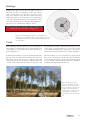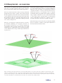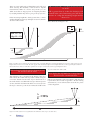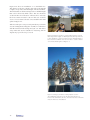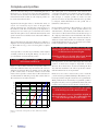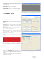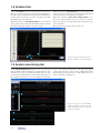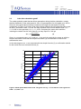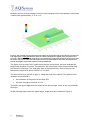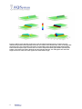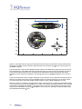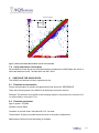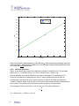
Download AQ500 User guide EN Dec 2013

AQ500 windfinder
User Guide
Version Date
Status
3
Third Edition
2013-12-13
Preface Revision 2013
The first major revision of AQ500 Wind Finder manual, version 3, was made in the autumn of 2013, a year and a half
after the initial release. Methods and recommendations have been refined since the last version came out in June 2012.
We've also had a lot of knowledge exchange with our users through our training AQademy. We recommend all users of
AQ500 to read this revised version of the manual. For experienced users, it may be sufficient to study the new Summary
/ Quick Guide at the beginning of the document and if necessary, seek more knowledge in the respective chapters. Below
we describe the changes that are made.
•
Summary / Quick Guide" is an entirely new section that in short describes how AQ500 should be handled and the
data analysed in order for the result of a measurement to be of high quality. The summary contains references to more
detailed information elsewhere in the document.
•
Chapter 1, "Introduction" is expanded with a section that describes the difference between systematic and random
errors and how they can affect a measurement.
•
Chapter 2, "Assessment of a site". We've added more examples of installations in the various categories. There is also
a section on what to look for and how to document a site visit with the purpose of finding suitable locations for an
AQ500.
•
Chapter 3, "Installing the System". Only small adjustments.
•
Chapter 4, "After Installation", is now focusing on the checks and service procedures you have to do to get a highquality measurement. The parts involving the analysis of data are moved to Chapter 5.
•
Chapter 5. "Analysis of Data" is to a large extent reorganized and improved with better examples of what a wind
analyst must look at to assess the quality of the measurement.
•
Appendix 8 is completely new and contains a simple and plain methodology for comparing observations from an
AQ500 with observations from another instrument.
•
Appendix 9 is new and includes a protocol that can be used in the field to document potential measurement sites.
•
Appendix 10 is also new and contains a recommended checklist to use during the installation of an AQ500.
We hope and believe that you will get much benefit from this updated manual.
AQSystem
2013-11-06
3
Contact details
Contact AQSystem by phone +46(0)8-776 40 86 or e-mail [email protected].
Order spare parts by sending an e-mail to [email protected].
Postal address
AQSystem Stockholm AB
Box 2135
SE-135 02 TYRESÖ
SWEDEN
Visiting address Stockholm
Mediavägen 18
135 48 TYRESÖ
Visiting address Gothenburg
Kyrkogatan 30
411 15 GOTHENBURG
AQademy
We offer training courses that covers usage and maintenance of your AQ500. They will help you to get the most out of
your investment in our high quality measurement equipment. Visit www.aqsystem.se and read more about AQademy!
4
Table of contents
Technical specification AQ500
6
Summary - Quick Guide for using the AQ500
7
1. Introduction
1.1 Principle of operation and geometry
2. Evaluation of a measurement site
2.1 Echoes from fixes objects
2.2 Steep terrain - an overview
2.3 Noise
2.4 Documentation of visited sites
2.5 Examples of installations
3. Installing the system
3.1 Installing the solpanels
3.2 Measuring the direction of the system
3.3 Start the system
3.4 Installation by helicopter or forest machine
15
17
19
20
25
27
28
30
38
39
40
40
41
4. After installation42
4.1 Communicate, remote control and download data
4.2 Recommended checks
5. Analysis of data
42
42
46
5.1 Data filtering by AQSystem
5.2 Normal data availability
5.3 Quality control of the data
5.4 Assessment of bias and conditioning
5.5 Scalar-vector correction
5.6 Compare the AQ500 with another data set
47
48
49
56
56
Appendices
Appendix 1 - User guide AQ Webviewer
Appendix 2 - User guide SODWIN-MCOM
Appendix 3 - User guide SODWIN.NET
Appendix 4 - Technical note: Conversion between vector and scalar wind values
Appendix 5 - Control your system remotely by SMS
Appendix 6 - Technical note: Quality control - data loss and conditioning
Appendix 7 - Technical note: Orographic deviation
Appendix 8 - Guide for comparing AQ500 data with other data
Appendix 9 - Site visit protocol
Appendix 10 - Installation protocol
56
5
Technical specification AQ500
The antenna
Number of transmitters
3
Transmitting frequency
3144Hz
Lobes
3
Angle between one lobe and the vertical line
15º
Lobe width
12º
Maximum output power from the speakers
300W*
The measurement
Highest measuring height
150 eller 200 m
Lowest measuring height
20 eller 50 m
Vertical resolution
5m
Mean value period
10 min
Wind speed range
0 – 30 m/s
Accuracy horizontal wind speed
+/- 2%**
Vertical wind speed range
Accuracy wind direction
+/- 2,2 m/s***
<5º
* The recommended output power during normal operation is 250W. Higher power will increase the risk of speaker
membrane failure.
** For wind speeds above 4 m/s compared to a cup anemometer in flat terrain with homogenous vegetation and after
correction for vector-scalar average difference. Read more about comparisons between AQ500 and cup anemometers in
appendix 8.
*** In the current version of AQ Webviewer and the latest version of MCOM.
6
Summary - Quick Guide for using the AQ500
AQ500 is a precision instrument and must be handled as such. In order to get useful measurement results you must follow
the recommendations in this manual. The following sections briefly describe how AQ500 must be used. Each section
contains a reference to further information.
General recommendations
•
Scout and document sites prior to every installation
•
Validate your AQ500 against a high quality met mast, in flat terrain with uniform vegetation, before and after every
measurement campaign
•
Always do reconnaissance and installation on different days
•
Document each installation
•
Never place two AQ500 transmitting at the same frequency closer than 800 meters
•
Perform service on your system at least every three months
•
A diesel heater is necessary for good data quality on sites where snow occurs
•
Data from an AQ500 is ready to use without additional filtering.
•
Make sure your wind analysis provider know how to
1. Assess whether an installation is good or bad
2. Detect if fixed echoes have affected the measurement
3. Check whether a scalar-vector correction is necessary
4. Check whether different data availability at different levels have introduced a systematic error in the measurement
Meteorology
Measurements
Statistics
It is essential to have knowledge in meteorology, measurements and statistics to get the most out of an investment in the
AQ500. AQSystem are happy to help you learn more about how AQ500 works and how it should be used through the
popular training course Aqademy.
7
Find a suitable location
The following must be documented / investigated when the suitability of a site for measurements with an AQ500 is
evaluated
•
Name/Description of the site
•
Position/coordinates
•
The acoustics on the site
•
Objects that potentially could interfere with the measurement - such as buildings, masts, turbines, trees and rock walls
•
Distance to neighbours
•
Transportation to and from the site
•
Visibility
•
Photos
•
Meteorological suitability and orography
•
Direction of the AQ500 - NOTE that the measurement quality may suffer if you try too have the solar panels facing
south at all costs
•
Read more in chapter 2
It is not the height of an object that determines how far from it the AQ500 can be placed withouth risk of
interference. The safe distance is determined by the maximum measuring height of the AQ500.
The figure below shows the three measurement lobes of the AQ500. The inner half sphere represents
the lowest measurement height and the outer half sphere represents the maximum measurement height.
Objects that can disturb the measurement, for example a met mast, must not be within the volume
between the two half spheres.
Lowest measurement level
Highest measurement
level
8
Install the AQ500
Document the installation using the installation protocol in appendix 10.
•
Position the system at the decided site and in the correct direction
•
Install the temperature-/humidity sensor
•
Level the system
•
Install the communication antenna
•
Install the solar panels
•
Measure the direction of the systemet
•
Turn the system on
•
Set the direction, output power and the clock (only GSM-communication)
•
Document the installation according to appendix 10.
•
Make sure that the communication works and that data is retrieved (GSM) or sent (WEBB) automatically
•
Make sure the temperaure sensor is working
•
Make sure that the loudspeaker diaphragm are ok (spectrum)
•
Read more in chapter 3
Never leave loose objects in the antenna compartment or in the generator area. These can vibrate and
disturb the measurement when the generator is running.
Some issues to think about when the AQ500 have GSM-communication
Change of name and direction
When the name and direction of a system is changed and data is downloaded from times before the change, the new
information will be in the heading of all downloaded files. The wind direction in the files is however based on the correct
settings at each ten minute period. Please note that you must keep track of when the instrument is moved. To reduce the risk
of mixing up different measurement campaigns we recommend that you empty the memory card between the campaigns .
Data retrieval with SODWIN-MCOM
There are some occasions when SODWIN-MCOM indicates that data is fetched without this being the case:
1.There are too many files on the memory card in the AQ500. Empty the card at least once a year, for example when
service is made. You will have to physically remove the card from the AQ500 and and insert it into a computer.
2.If the memory card in the AQ500 is empty.
The site name must only contain letters and numbers. Special chracters such as @ ’ ` etc. can affect the
data retrieval.
9
Follow up the measurement
Your measurements must be continously monitored for any deviations to be detected at an early stage.
Without the necessary follow up there is a risk that you loose data, which in turn increases the uncertainty
in the evalutation of the wind resource.
Follow up of an installation
In addition to the basic functionality checks made in connection with the installation, the measurement must be followed
up one to two weeks after installation. The purpose of the check is to ensure that everything works as expected and to
investigate if the measurement is affected by fixed echoes. Fixed echoes can be dependent on wind direction; waiting one
to two weeks will increase the wind directions present in the data. You should look at
•
The temperature – the measurements of the wind speed will not be correct without valid temperature observations
•
Complete profiles - very good for detecting fixed echoes if averaged over days or longer periods.
•
The spectrums – to make sure that the speakers work as expected. Never use higher speaker output power than 250
W to avoid speaker diaphragm failure.
Weekly checks
After the initial follow-up one to two weeks after installation, the measurement must be monitored weekly so that
deviations to normal operation are detected at an early stage. You should look at
•
The temperature – the measurements of the wind speed will not be correct without valid temperature observations
•
The battery voltage - make sure that the power pack works as expected
•
The fuel level - refuel before the tank is empty to avoid battery damages
•
The spectrums– to make sure that the speakers work as expected. Never use higher speaker output power than 250
W to avoid speaker diaphragm failure.
Monthly checks
A simple report including a basic quality check should be made once every month. You should look at
•
The data availability
•
Time series of temperature, wind speed and wind direction
•
The distribution of wind speed and wind direction
•
Complete profiles - very good for detecting fixed echoes if averaged over days or longer periods.
Read more in chapter 4
10
Take care of your AQ500
In addition to data monitoring, it is also important that your AQ500 is maintained according to current service
recommendations. This will minimize the risk of lost data. Read more in Chapter 4.
Power supply
AQ500 contains a conventional diesel engine and standard
lead-acid batteries. These components are worn in the same
way as other engines and batteries. The service life of the
diesel engine is about 3000 hours. The batteries will work
satisfactorily under normal operating conditions for at least
three years. You must make sure to maintain both the diesel
engine and the batteries. Neglect or improper maintenance
will result in irreparable damage. As a result, you will lose
data, and must conduct costly repairs.
If the engine does not run in the summer we recommend
that you manually start it once a month. This can be
done remotely, see appendix 5 for systems with GSM
communication and appendix 1 for systems with webcommunication.
Sound attenuation material
The sound attenuation material, a kind of foam rubber,
in the antenna compartment wears when exposed to
the elements. After a few years this may affect the wind
measurements if the sound is reflected inside the antenna
compartment. The most critical area is on the upper part
of the walls which coincides with where the foam is the
most exposed to ambient conditions. Initially, the material
is 30 mm thick. When the thickness is approaching 15 mm,
it is time to replace it. The foam has a wavy texture and
the thickness is measured from the back side (glued to the
wall) to the peaks of the waves. The pictures to the right
show examples of new and undamaged foam (top) and
completely worn foam (bottom).
The temperature sensor
A working temperature sensor is necessary for correct wind measurements. Since the speed of sound in air is temperature
dependent, incorrect temperature means that the readings will come from the wrong height. As a rule of thumb a deviation
of more than ten degrees means that the error in the measurement becomes significant.
Never mount the temperature sensor above the dark solar panels as this will make the temperature too high!
11
Analysis of data from an AQ500
It is important that the recommendations from AQSystem is followed when the observations from the AQ500 is evaluated.
•
Observations from the AQ500 are ready to use – never filter data on signal-to-noise ratio or on the presence of
standard deviation.
•
The data availability on turbulence data is significant less than for wind speed – this does not affect the quality of the
wind speed!
•
Spikes (heavily deviant, occasional observations) in the wind speed can occur a few times during a month – these
observations must be removed before the analysis is made.
•
The AQ500 measures the vector mean wind speed – investigate if a conversion to a scalar wind speed is necessary!
•
Conditioning errors can occur if data is missing – investigate if they are significant on the measurement levels of
interest
•
Read more in chapter 5.
Never use a numerical model to validate the quality of Your
measurement!
We measure to decrease modeling uncertainty!
12
Compare data from an AQ500 with another set of observations
When data from an AQ500 is compared with measurements made in a nearby (within a few hundred meters) met mast,
it is important to
•
make a thorough quality check of the AQ500 data
•
make a thorough quality check of the met mast data
•
synchronize the data sets
•
only make the comparison with concurrent data
•
remove sectors from the comparison when the AQ500 or met mast is disturbed
•
compare the same levels - do not compensate for difference in height between the met mast foundation and the
location where the AQ500 have been installed
•
compensate for vector - scalar differences
•
calculate the uncertainty of the difference
•
read chapter 5.6 in the AQ500 User guide before the comparison is made
13
14
1. Introduction
The AQ500 is a remote sensing instrument of type
sodar (Sonic Detection and Ranging). With sound,
the AQ500 can measure the wind up to 200 meters
above ground. The sound used has a frequency of
3144 Hz. This corresponds to key 83 on a regular
piano with 88 keys.
Developed in Sweden, the AQ500 is made for use
in tough winter climate. But operation is of course
not limited to the cold part of the year. The power
supply consists of both a diesel generator and
solar panels which makes the operation during the
summer months almost free of emissions.
The instrument is placed in a trailer that also contains the
power supply for reliable operation. The trailer makes the
AQ500 easy to move with a normal sized car. The AQ500
can be used as the sole instrument in a wind measurement
campaign or in combination with a met mast. Compared
to a met mast, you will get measurements on many more
levels.
Figure 1-1 The three speakers/microphones (black) together with
the reflective parabolic disks (white) that form the antenna device in
AQ500
Meteorology
During the winter, the operation is improved by a diesel
heater which preheats the generator before it starts. Excess
heat from the diesel heater is not wasted but used to melt
any snow and ice in the space where the sodar antenna is
placed. As a user, you do not need to worry about freezing
instruments or lacking observations during the cold time of
year. The diesel heater is an option that can be installed in
the factory or retrofitted in the field.
The design of the antenna unit, which creates the sound
pulses, is robust and has no moving parts. The speakers are
fitted upside down, see Figure 1-1 , and therefore will not be
filled with snow. The snow settles instead on the parabolic
surfaces that are equipped with heater elements and where
excess heat from the diesel heater is also directed.
The AQ500 is a precision instrument and must
be treated as such in order to function properly.
The result you get depends to 50 percent on the
instrument and to 50 percent on how you use it.
Measurements
Statistics
Figure 1-2 The three areas of expertise that are important when
data from an AQ500 is analysed.
To increase traceability, we recommend that you validate
your AQ500 against a good met mast in flat terrain and
with homogeneous vegetation before and after each
measurement campaign.
In addition to using the instrument correctly, you also
need to understand what the instrument delivers and how
to present this in an understandable way. It is important
to have knowledge of meteorology, measurements and
statistics when analysing and evaluating data. This is
illustrated by Figure 1-2 and is of course not limited to
AQ500, it is equally important when measurements made
in a mast or with another remote sensor are analysed.
15
Glossary
Antenna part/antenna compartment – the compartment
in the trailer where the sodar antenna is located.
Diesel heater – preheats the generator in the AQ500
before it starts. Extends the life of the generator as cold
starting is avoided. Excess heat is directed to the antenna
compartment and ensures that the antenna is free of snow
and ice formation is avoided.
Measurement lobe – the cone shaped volume that
measurements are made in. The AQ500 measures in three
lobes, Figure 1-3.
Orography – the science of the earth's surface forms.
Orographic deviation – a deviation in the measured wind
speed due to the orography in the immediate surroundings
of the AQ500.
Doppler effect – the frequency of a transmitted sound is
perceived differently if the sound source moves toward or
away from the listener.
Signal-to-noise ratio – the relation between the echo that
the AQ500 logs and the noise from the surroundings.
Fixed echo – an echo from an non moving object, for
example a tree, a house wall or met mast.
Sodar antenna – the part where sound pulses are created
and the echo is logged. Three-axis antenna, Figure 1-1.
Remote sensing instrument – an instrument that makes
measurements over a distance by analysis of, for example,
echoes of sound (sodar) or reflections of light (lidar). Radar
and instruments mounted on satellites are also remote
sensing instruments.
Spectrum – Breakdown of a wave motion such as sound
into frequencies or wavelengths.
Atmospheric echo – an echo from the atmosphere. The
echo occurs when the sound is reflected in small temperature
variations, which always occur in the atmosphere.
16
Webviewer – AQSystem’s web-based system that makes
it easy for the AQ500 owner to monitor and manage the
measurement.
Zenith angle – The angle between the vertical line and the
centre of the measurement lobe, Figure 1-3
1.1 Principle of operation and geometry
AQ500 measures the wind’s directional components, two
horizontal and one vertical, by transmitting sound into the
atmosphere. The sound is reflected by small temperature
variations. These moves with the wind and the reflected
sound have, due to the Doppler effect, a different frequency
than the transmitted. The difference between the transmitted
and received (reflected) frequency is used to calculate the
wind speed and direction.
AQ500 is based on monostatic technique. This means
that the speaker that emits the sound pulses also acts as a
microphone and listens to the reflected sound. In order to
15°
calculate the wind’s three components, AQ500 is equipped
with three separate speakers/microphones that emit sound
in three directions. The sodar antenna is shown in Figure
1-1.
The geometry for the whole system is shown in Figure 1-3.
The sound that AQ500 emits spreads in a cone-shaped
volume, which we call the measurement lobe. The centre
of the lobe inclines 15° to the vertical line, and has a width
of 12º. The angle between the three measurement lobes is
120º. The measurement lobes are labelled A, B and C with
A in the direction of the trailers drawbar.
120°
6°
C
A
B
Figure 1-3 Left: The emitted sound spreads in a cone-shaped volume, which we call measurement lobe. The centre of the cone is inclined 15°
to the vertical line. The half angle of the cone is 6º. Right: The sound is emitted in three directions separated by 120º.
17
1.1.1 Systematic and random errors
All measurements contain errors. Measurement errors can
be split into systematic and random. One example is a worn
folding rule where the first millimetre (mm) is missing. Each
time it is used, the measurement is one mm too long. It has a
systematic error of plus one mm. An example of a random
measurement error is the reading error. Since the folding
rule is graduated in mm the reading error is about one
mm. On one occasion you read one mm too much and the
next time one mm too little, or even just right. By repeating
the measurement several times and take an average, the
influence of the random measurement error is reduced. It
evens out. After many measurements it will be negligible.
The systematic measurement error is not affected by taking
an average, it remains unchanged.
In some situations you have to weigh systematic and random
measurement errors against each other when designing
a measuring instrument. Remote sensing instruments for
wind is such an example.
Remote sensing instruments for wind - sodars and lidars use instant measurements of wind in various measurement
volumes above the instrument. The angle between the
vertical and the centre of the measurement volume, the
zenith angle, is shown in Figure 1-3. A small zenith angle
gives a small distance between the measurement volumes.
This is a big advantage in complex terrain since the wind
above the remote sensor follows the terrain and thus
follows curved paths as shown in Figur 2-9. A curved wind
field gives a systematic error in the wind measurement. This
error increases with the distance between the measurement
volumes, i.e. with zenith angle. A small zenith angle also
gives a weaker signal and thus a larger random error or
noise.
When designing a remote sensing instrument one must
therefore weigh the advantages and disadvantages of a
certain zenith angle to each other. In the design of AQ500,
we prefer a smaller zenith angle for the following reasons.
A small zenith angle gives a small systematic error
but higher noise.
The systematic error can not be eliminated by
averaging, while the noise will completely disappear
by averaging.
Since it is the average that is of interest in wind resource
applications, this is the correct balance.
Lidars has about twice the zenith angle compared to the
AQ500 and thus a larger systematic error in a given terrain.
Lidars often have a lower noise level, which in principle is
a purely cosmetic benefit and not an advantage in a wind
resource context.
1.1.2 AQ500 measures the vector wind
AQ500 calculates the horizontal wind as the two
perpendicular components of a vector, such as the northsouth component and the east-west component. This is
done many times during a ten minute period whereupon
the component mean is calculated. The result is called the
vector mean wind speed. The vector mean wind has both
magnitude and direction.
A cup anemometer gives the wind speed directly. The
anemometer is logged many times in a ten minute period
and then an average is calculated. The result is the scalar
mean wind, having a certain magnitude. The wind direction
can't be measured by the anemometer.
A vector has both a length and a direction while a scalar
only have a length. The vector and scalar wind are equal
in a smooth, non-turbulent, wind. In reality, turbulence is
always present and hence there is a difference between the
vector and scalar wind. The difference depends on how
turbulent the wind is, the more turbulence, the greater the
18
difference.
The vector mean wind is always slightly weaker than scalar
mean wind. That means that the AQ500 measures a slightly
weaker wind than a cup anemometer.
The difference is not an error but a consequence of the
fact that the average wind speed by tradition is defined
as the scalar value. As the wind turbines power curves
traditionally is verified against cup anemometers it is
sometimes necessary to adjust the wind speed measured
by an AQ500.
In most cases, the difference between the vector
average and the scalar average is small or negligible.
Appendix 4 contains a method för conversion from
vector to scalar.
2. Evaluation of a measurement site
In the introduction it was mentioned that the results of a
measurement with an AQ500 to 50 percent depends on the
instrument and to 50 percent on how it is used. A large part
of the 50 percent related to the usage consists of finding
a suitable site for the instrument. This chapter is devoted
to the suitability assessment of a site with respect to the
AQ500.
Always strive to install the AQ500 at a site free
from disturbances. This will avoid questions to be
raised concerning the validity of the measurement
when the data is analyzed.
Note that we only discuss the suitability of a site with
respect to the AQ500 in this chapter. Where in the project
area the measurement should be made to maximize the
benefit is specific to each project and is not covered here.
Sometimes there is a need to measure on locations that
are not ideal. In such cases we recommend that the
planning of the measurement campaign and installation
is made together with the consultant that will analyse
the measurement and that all involved are informed, for
examples. investors, on the priorities. It is also important
to follow up the measurement and take action if any kind
of disturbance is found.
19
2.1 Echoes from fixes objects
AQ500 have two measurement interval configurations:
20-150 meter or 50-200 meter. A timer starts when a sound
pulse has been sent. The AQ500 starts to listen for echoes
when enough time has passed for the sound to travel to the
lowest measurement height and back again. The AQ500
stops listening when enough time has passed for the sound
to travel to the highest measurement interval and back
again.
Echoes from objects in the surroundings, such as trees,
buildings or a met mast, which reaches the AQ500
during the listening phase may cause a deviation in the
measurement. Echoes that arrive before the AQ500 starts
to listen or after the AQ500 has stopped listening do not
affect the measurement.
Objects that are closer than the lowest measuring
height and farther away than the highest measuring
height do not affect the measurement.
This means that there is a volume within which there
should be no obstructions. The inner half sphere in Figure
2-1 represents the lowest measuring height while the outer
represents the highest measuring height. The volume
between the two half spheres must be free from interfering
objects.
It is not the height of the object that determines
how close an AQ500 can be placed. The distance is
determined by the maximum measuring height of
the AQ500
If an object reflects the sound emitted by the AQ500 or
not depends on the size of the object in relation to the
wavelength of the sound. The wavelength of the sound
that the AQ500 sends out is around 10 centimetres. To
reflect this, an object must have an extension of about 15
centimetres. Small trees and thin twigs are therefore not
reflecting the sound. Bushes and low and young conifer
can even be advantageous to have around the measurement
site since they are good sound absorbers and don't reflect
the sound.
Lowest measurement level
Highest measurement
level
Figure 2-1 The cones are the AQ500 measurement lobes. The inner half sphere represents the lowest measuring height while the outer
represents the highest measuring height. The volume between the two half spheres must be free from interfering objects.
20
That objects closer than the lowest measuring height can't
influence the measurement is not entirely correct. Of course,
it is absolutely essential that you do not place the AQ500 so
that any of measurement lobes goes into an object.
As mentioned, the zenith angle is 15 ° and the width of the
lobes is 12 °. The angle between the lobes are 120 °, see
Figure 1-3. The vertical distance between the outer edge
of the lobes and the ground at different distances from
the AQ500 is shown in Figure 2-2. Because of the small
zenith angle, the AQ500 do not require a large open area
in order to be deployed. This is of course beneficial when
installations in the field are made.
Distance
the outer
part of
the
Höjd till to
lobens
ytterkant
(m)
lobe (m)
78
65
52
39
26
13
Horizontal
distance
(m)
Horisontellt
avstånd
(m)
30 25
20 15
10
5
Figure 2-2 The vertical distance between the outer edge of the lobes and the ground at different distances
from the AQ500.
21
How to avoid fixed echoes
To avoid fixed echoes, it is important that a site visit is made
prior to the installation and that the measurement data
is carefully monitored after the installation. Read more
about how to check the data in Section 5.3. The goal of
the installation must be to not have any disturbing objects
in the volume between the two half spheres in Figure 2-1.
Examine the acoustic environment on a site by clapping
your hands and listen for echoes. Estimate the time it takes
for the echoes to reach you and try to determine what causes
them. If possible, avoid places with too much echoes. Read
more in the section "Documentation of visited sites" below.
It is not always possible to keep the volume between the
half spheres completely free from objects. If that is the case,
it is important not to point any of the lobes towards the
object. Instead AQ500 should be positioned so that the
lobes are directed on opposite sides of the object. This is
illustrated in Figure 2-3.
Figure 2-3 Avoid pointing any of the
lobes towards an object if it is closer
to the AQ500 than the maximum
measurement height. The red arrows
show the direction of the lobes.
It's easy to find the heights that could be affected by an
object between the two half spheres. An example is shown
in Figure 2-4. An AQ500 is at A. At B is a met mast that
is 100 metres high. The horizontal distance between the
AQ500 and the mast is 120 metres. The distance between
the AQ500 and the top of the mast can be calculated, using
the Pythagorean theorem, to 156 meters. This means that
it is the measurement levels between 120 meters and 155
meters which potentially could be affected by fixed echoes.
The height range that an object of a certain height can affect
decreases with the distance to the object. A 20 meter tall
tree at a distance of 50 meters can affect a height interval
of nearly five meters while the same tree 150 metres away
can affect a range of just over one meter.
If an AQ500, for some reason, is installed at a site that is
not ideal it is important to make a check one to two weeks
22
after the installation and take appropriate measures if it is
found that the measurement is disturbed.
156 m
A
120 m
100 m
B
Figure 2-4 Using the Pythagorean theorem, it is easy to find the
heights that can be affected by a fixed echo.
Buildings
Buildings have large surfaces that can reflect sound very
effectively. If there are buildings nearby, the starting
position is the same as for other types of objects: do not
deploy the AQ500 closer than the highest measuring
height. If, however, you still do this, we recommend that
you position the AQ500 against a corner without directing
any of measurement lobes towards the building Figure 2-5.
The purpose is to minimise the reflective surface.
Avoid to position an AQ500 so that buildings are
within the critical volume in Figure 2-1
Figure 2-5 An AQ500 that, against our recommendations, is
installed close to a building should be placed against one corner of
the building with the lobes on either side. This will minimize the
reflecting surface.
Trees
Trees with large and bare stems are good sound reflectors
and should be avoided in the critical volume in Figure 2-1
. An example of a tree line that may cause a fixed echo is
shown in Figure 2-6.
fir with plenty of needles on branches and twigs are good
at absorbing sound and therefore good for the acoustic
environment. Nevertheless, it is important to visit all sites
and not make a decision based solely on maps and photos.
In the background there is a spruce plantation that marks
the edge of the clear felled area. Transitions between clear
felled areas and forests can act as a reflective wall, thus
causing a fixed echo. The probability is highest if the forest
consists of trees with mostly bare stems. Young spruce and
The site in Figure 2-6 was considered very inappropriate
due to echoes from the trees in the centre. If a site like this
is used despite the strong echoes, the measurement must
be very carefully checked and alternative sites should be
evaluated if the AQ500 must be moved.
Figure 2-6 Bare, large stems
can cause disturbing echo. The
distance to the trees is about 60
metres. A curtain of spruce in the
background, about 100 metres
away, can act as a reflective wall
and should also be taken into
consideration when assessing the
site.
23
Slopes strewn with stone boulders
Do not deploy an AQ500 beside a slope strewn with rocks
and stone boulders. An example of such a site is shown in
Figure 2-7. If you still have to position the AQ500 here, you
should position it as close to the stone boulders as possible
and do not direct any of the measurement lobes towards the
trees. Figure 2-8 shows another example of a position with
large stone boulders on a slope that may adversely affect
the measurement.
Figure 2-7 If possible, you
should avoid bare stems and
stone boulders in the critical
volume in Figure 2-1
Figure 2-8 A slope with large
stone boulders can cause fixed
echoes. If possible, avoid sites
like this.
24
2.2 Steep terrain - an overview
Steep terrain can sometimes affect the wind measurement
and cause orographic deviation. This section contains a
short overview, more details can be found in appendix 7.
The reason why the terrain can have an impact is that the
AQ500 measures in three volumes and assumes that the
flow through these is linear. All remote sensing instruments
(sodar and lidar) that use Doppler technology must make
this assumption. The more curved the airflow, the less the
validity of the assumption of linear flow and the greater the
error can be, see Figure 2-9.
However, you should not exaggerate the risk, it needs to
be extremely undulating for orographic deviations on
the measured wind speed to be a problem. AQ500 has
an unusually small orographic deviation due to its small
zenith angle of 15°. Many other remote sensing instruments
(sodar and lidar) have a larger zenith angle and therefore
a greater error.
The deviations that nevertheless occur can to a large extent
be corrected afterwards by means of computer simulations.
However, as far as possible, you should avoid relying on
computer models for correction. An important reason to
measure the wind is to avoid having to rely on computer
models that suffer from significant uncertainties. Applying a
large computer calculated correction on the measured wind
to some extent cancels out the benefit of a measurement.
Our recommendation is therefore to attempt to choose a
site where deviations caused by orography are small.
In the following section we show how to determine whether
the site is suitable or whether a subsequent adjustment of
the measurements should be made.
Figure 2-9 At the top the wind is shown above level ground. The wind does not vary, but is the same for all three measurement lobes. The
problem to calculate the wind’s three components is well determined. Below a situation where the instrument is positioned on undulating
ground is shown, which gives a curved airflow. The wind is different at the three measurement lobes. In principle the variation is impossible
to calculate. The difference in wind in the three lobes will cause a deviation in the calculated wind.
25
If H is at most 10% of Δ then the deviation will
be small
There are some simple rules of thumb that can be followed
when assessing the suitability of the terrain for AQ500
measurements. When it concerns steep terrain you can
define areas that are inappropriate for AQ500 placement
by studying detailed maps before going to the project area.
If the measuring height H is much greater than, or much
smaller than the terrain’s typical height variation Δ, then the
deviation will be small.
If H is greater than 4 Δ then the deviation will
be small in the case of measuring on a hill. If you
measure on a ridge the measuring height must be
about 15 Δ.
This is illustrated in Figure 2-10.
H<
Δ
10
H
Hill: H > 4∆
H>4Δ
Ridge: H > 15∆
H
Δ
Δ
B
B
Figure 2-10 The arrows symbolise the measurement lobes on AQ500. When the measuring height H is at most 10% of the terrain’s typical
height variation Δ the error is small. The same applies if the measuring height is 4 times higher than the terrain’s typical height variation if
the measurement is made on a hill. The equivalent for a ridge is 15 times the terrain’s typical height variation.
If the inclination of the slope is less than 10 percent,
the deviation will be small.
The inclination, Λ, is calculated as the height of the slope
Δ divided by the width of the slope B, Λ = Δ / B, see Figure
2-11. Note that the breath of the slope in the direction of
the wind must be used. If the hill is steeper than 10 percent
(Λ >0.1) then the instrument should be moved away from
the slope so that it is positioned 3-4 times the width of the
slope downstream of the same.
Never deploy the AQ500 below a steep slope, the
deviation have a maximum there.
Fully prepared examples of how an estimate of the deviation
is performed can be found in appendix 7. If after making
an estimation you are still uncertain about the site, please
contact AQSystem.
∆
— <10%
B
Δ
B
Figure 2-11 The deviation is not significant if the inclination of the slope is less than 10%.
26
2.3 Noise
In general, noise from the surroundings is not a problem.
Nevertheless it is still a good idea to take this into
consideration when choosing your site.
Roads and industries
AQ500 have been installed next to heavily trafficked
roads, both in Sweden and abroad, without this causing
any disturbances.
If large amounts of data are lost, there is a risk for
conditioning errors, see Section 5.4 and appendix 6. Avoid
sites where the environment causes loss of data..
The quality number, defined as the signal-to-noise ratio
times 10 and that is included in the data files from the
AQ500, can be used to examine if the noise affects the
measurement. If it varies with the diurnal variation of the
noise and drops below 21, which means that the data is
rejected, the noise is a problem.
Loose objects
Loose objects in sodar trailer can cause disruptive noise if
they begin to vibrate when the generator is running.
The solar panels should under no circumstances be stored in
the antenna compartment during measurements. However,
it's a great place for them during transport.
Do not use the AQ500 for storage. Remove
equipment not in use and make sure that the tools
in the trailer are stored in such a way that they can't
cause disturbing vibrational noise.
Guy wires from large masts
Be careful if you intend to position your system near large
communication masts with guy wires. In conditions with
high winds, a tone can be created by the guy wires. If the
tone is close to the sound transmitted by the AQ500, 3144
Hz, measurements cannot be made at the site.
27
2.4 Documentation of visited sites
It is important to be well prepared when potential
measurement sites is visited and evaluated. In addition to
proper equipment, you must have a plan of what to look at
when you come to a site. It is easy to forget or mix sites up,
especially if you visit many places. A good documentation
routine makes the job easier. Appendix 9 is a suggested
protocol that can be used in the field. We use this when we
describe how a site assessment prior to measurement with
an AQ500 should be done.
Never plan reconnaissance and installation of an
AQ500 on the same day. After completing the
reconnaissance, impressions should be processed
at the warm and dry office before a final decision is
made. Otherwise the risk is high that a less suitable
location is chosen because of stress.
Name
Give each visited site a name that allows you to easily recall
it when you write the report at home. This is especially
important when visiting several places at the same time.
Coordinates
Use a GPS to determine the position and note this along
with what kind of coordinates it concerns. If you don't have
a GPS be sure to mark the location on a map.
We recommend that you always mark the location
on a map already in the field, regardless of whether
you have a GPS or not
This minimizes the risk of deploying the AQ500 on the
wrong site if the GPS for some reason is incorrect.
Acoustics and objects
Check the site's acoustic environment by clapping your
hands in different directions. Listen for echoes and try to
identify what causes them. The sound moves about 330 m /
s. An echo that comes back after one second originates from
an object that is about 150 meters away. Try to determine
what cause the echoes. Remember that echoes coming from
objects that are closer than the lowest measuring level or
farther than the highest measuring level does not affect the
measurement. This is illustrated by Figure 2-1.
Not all echoes that the human ear can hear will disturb the
measurement. But to minimize the risk, sites with heavy
echoes should be avoided. Fixed echoes can be identified in
the data. Read more about this in Section 5.3.
28
Distance to neighbours
Note the distance and direction to any residential building.
AQ500 emits a sound that is equivalent to about key 83
on a standard piano with 88 keys. Thus it is audible to
the human ear. AQ500 emits about one sound pulse per
second around the clock. It is thus important to ensure
that no permanent or summer houses that can be disturbed
are nearby. How far the sound travels depends both on
the weather situation and on the surrounding terrain. The
sound may be heard several hundred meters away from the
AQ500 during a calm and quiet summer night in an open
landscape, while it is not perceived by the human ear at
all in windy situations because of the background noise.
Therefore, there is no guidance regarding the distance to
residential buildings. We recommend that you inform and
have a dialogue with residents in the area to avoid the risk
of having to move the AQ500.
Transportation
Describe the way to and from the site. It is not only when
you install and uninstall the AQ500 that it must be possible
to come to the site. Service and refuelling must be carried
out at regular intervals. What happens to the road after a
few months of autumn rain? Will it be plowed or is there a
need for a snowmobile in the winter?
Describe the soil conditions on the exact position where
the AQ500 should be installed. Will the support legs stand
on firm ground or is there a need for boards or gravel to
stabilize?
Visibility
How exposed is the AQ500 for people passing by? Solar
panels, diesel engine, diesel and batteries are theft-attractive.
Take appropriate actions for the location you have selected.
It may be a matter of putting up a road barrier, use
camouflage netting or install a surveillance camera. Please
note that cameras may require a permit.
Direction of the system
Enter a recommended direction of the system. The system's
direction is indicated by the drawbar, read more about how
you measure direction in Section 3.2.
Note that the most important thing is that the
measurement is good, not that the solar panels are
facing south. The direction of the panels has a low
priority compared to all other aspects of the site.
Pictures
Document the surroundings with photographs in at least
four directions. By including a compass on the photos
you will have information about both the direction and
the environment at the same place, see Figure 2-12 for an
example. Note in the protocol if there is anything on any
image that especially should be considered.
TIP. Take a picture of the protocol for the site both
before and after you take images of the surroundings.
This makes it easy to know to what site they belong.
Figure 2-12 By including a compass on the photos you
will have information about both the direction and the
environment at the same place.
Meteorology and orography
The meteorological suitability of a site is project specific
and is not covered here. The assessment should be made as
part of the preparations before the site visit. Notes can be
made on the protocol, this way all information about the
site is at the same place.
Steep terrain can affect the measurement. This is project
specific. But since it also is related to the measurement
principle of the AQ500 there are some rules of thumb in
section 2.2 that can be used to assess if the impact of the
terrain is significant or not. Appendix 7 contains a more
detailed description of the terrain effects and a simple
method that can be used to calculate the maximum effect
on the measurement. The assessment should be done as part
of the preparations before the site visit. Notes can be made
on the protocol, this way all information about the site is
at the same place.
29
2.5 Examples of installations
This section shows examples of installation sites and how
you should deal with them. They are categorised from 1 to 5
Category 4 - less good location for an AQ500, avoid if
possible
Category 1 - excellent location for an AQ500
Category 5 - not suitably for an AQ500
Category 2 - very good location for an AQ500
Note that the categorization is of the locations suitability
for measurements with an AQ500, not of the suitability
from a project perspective.
Category 3 - good location for an AQ500
Category 1
Figure 2-13 shows four examples of sites in Category 1.
The landscape is open in all directions and there are no
objects in the volume between the half spheres in Figure
2-1 that can cause fixed echoes. The terrain is without steep
slopes in all four cases which mean that there is no risk
of orographic deviations, see Section 2.2. These are four
excellent measurement sites.
Figure 2-13 Four examples of sites in Category 1. There are no
disturbing objects within the volume in Figure 2-1. The terrain is
without steep slopes.
30
Category 2
To the right in Figure 2-14 an example of a site in category
2 is shown. This is a very good measurement site. It is
open in all directions, the only thing that could potentially
interfere is the measurement mast that can be made out
on the right of the photo. The mast is 80 metres high and
the horizontal distance between the AQ500 and the mast is
140 metres. The distance between the AQ500 and the top
of the mast is 161 metres. This is shown in the diagram to
the left of i Figure 2-14 where the AQ500 stands at A, while
the mast is at B. Accordingly, it is at measurement heights
161 m
A
140 m
between 140 and 160 metres that the mast can interfere.
In order to minimise the risk of interference, none of the
measurement lobes should be directed towards the mast
and after installation, you should check the measurement
data for signs of fixed echo at the heights that can potentially
be disrupted, see section 5.3. If it becomes obvious that
the mast causes interference, the most effective measure
is to move the AQ500 further from the mast, preferably
further away than the maximum measuring height so that
it becomes outside of the volume described in Figure 2-1.
80 m
B
Figure 2-14 RIGHT: An example of a site in category 2. Here is a small risk that the mast may interfere with the measurement, otherwise
there are no sections of terrain that can cause problems, nor any disturbing sound sources. LEFT: The mast can, if it causes fixed echo,
interfere with the measurement at heights between 140 and 160 metres.
In Figure 2-15 young pines with plenty of needles that
are very good at absorbing sound is shown. The acoustic
environment at sites where the vegetation consists of
homogeneous young pine is often very good. Hence it is
often very good for measurements with an AQ500. Young
spruce without exposed stems, as in Figure 2-16, is also
good at absorbing sound. Sites like theese are often in
category 2..
Figure 2-15 Category 2. Young pine trees, in this case 2-4 metres
high, are excellent sound absorbers and sites like this is often
acoustically good.
Figure 2-16 Category 2. Fir trees with plenty of needles and without
exposed stems are good sound absorbers.
31
I Figure 2-17, Figure 2-18 and Figure 2-19 shows further
examples of measurement sites in category two. They
have the following in common: no steep terrain slopes
and vegetation that mainly consists of young coniferous
forest that is good at absorbing sound and minimizing the
probability of fixed echoes.
Figure 2-17 Category 2. The low, sound absorbing vegetation in the
background is within the two half spheres in Figure 2-1. The higher
trees are closer than the lowest measuring height and cannot cause
fixed echoes.
Figure 2-18 Only thin trees that does not reflect the sound emitted
by the AQ500 and flat terrain make this a category 2 site. The
young conifer are good sound absorbers and favourable to have in
the volume between the half spheres in Figure 2-1
Figure 2-19 Category 2. Young spruce is a good sound absorber.
This site is almost in category 1, but there are occasional taller trees
further away that can cause reflections..
32
Category 3
In Figure 2-20 it is the tall trees 40 metres away, partly
with bare stems, in the background that need attention.
Their upper parts extend into the volume between the half
spheres in Figure 2-1. You need to direct the lobes on either
side of the trees when installing in these conditions. It is
important to study the measurements after installation.
If the trees affect the measurement you should consider
moving it.
Figure 2-21 shows a site where trees stand very close to the
AQ500. At tight sites like this, it is important to make sure
that the lobes have a free line of sight, see Figure 2-2. You
should also direct the system so that the lobes points on
either side of the trees. A thorough follow up of the data is
also important, see Section 5.3.
At the site in Figure 2-22 it is the spruce curtain in the
background, 60 metres away, that needs to be considered.
If the spruce, which are in the area between the half spheres
in Figure 2-1, have bare stems, it may act as a reflective wall.
Follow up of the data is very important.
Figure 2-21 Category 3: The birch trees are very close. The lobes
must have a free line of sight and be pointed on either side of the
trees.
Figure 2-23 shows a tight place with a mix of acoustic
favourable conifers and less favourable deciduous trees
with bare trunks. It is important that the lobes have a
free line of sight and that the measurement is monitored
carefully.
Figure 2-22 Category 3. The spruce curtain in the background may
act as a reflective wall.
Figure 2-20 A site in category 3. Point the lobes on either side of the
trees to avoid disturbances.
Figure 2-23 Category 3. A tight site with a mix of acoustic favorable
conifers and less favourable deciduous trees with bare trunks. It
is important that the lobes have a free line of sight and that the
measurement is monitored carefully.
33
Figure 2-24 shows a typical location in Category 3. It is
a turnaround at the end of a road surrounded by trees of
varying species and age but with predominance of young
trees with thin stems. Sites like this are good for measuring
with an AQ500. But as with all other installations, it is
important to follow up the results to make sure that no
interference occurs.
The installation in Figure 2-25 is somewhere between
Category 3 and Category 4. The spruce adjacent to the
clear-felled area consists of rather big trees with bare and
exposed stems. The forest edge is extending diagonally
away from the AQ500 which mean that echoes can come
from several different distances and thus affect a wider
range of the profile. In this case, there were no strong echoes
and the follow-up showed no signs of fixed echoes. On sites
like this, it is sometimes better to place the AQ500 as close
to the forest edge as possible so that it is within the inner
half sphere in Figure 2-1.
Figure 2-24 A typical site in category 3. A turnaround surrounded
by trees of varying type and age. This is in general a good site, but
proper follow-up is, as always, important..
Figure 2-25 Category 3. The forest in the background consists of
tall spruce with bare stems. The diagonal stretch with respect to the
AQ500 means that echoes can come from several distances and thus
affect a wider range of the profile.
34
Category 4
Figure 2-26 shows an example of a site in category four. The
site is surrounded by pine trees. The closest is within the
inner half sphere in Figure 2-1 but since the forest farther
away consists of the same type of trees with many bare
stems , there is a high probability of fixed echoes. We advise
against measuring at sites similar to this. If a site like this
is used, the follow-up, including looking for signs of fixed
echoes, is very important, see Section 5.3. A tip is to have
a back-up site prepared before the installation so that the
AQ500 can be moved without delaying the measurement
campaign if signs of fixed echoes are found.
Figure 2-27 shows a site with high, bare stemmed trees
and exposed rock. We advise from using this site. If that is
not possible, put the AQ500 as close to the exposed rock
as possible without pointing any of the lobes towards the
trees. The distance to the trees will then be between 20 and
30 metres, hence they are inside the inner half sphere in
Figure 2-1.
Figure 2-28 shows an AQ500 deployed in a young pine
forest that is good at absorbing sounds. The reason that
this site is in category four is the met mast about 120 meters
behind the AQ500, difficult access to the site and complex
terrain that can cause an orographic deviation.
Figure 2-26 Category 4. Lots of trees with bare stems that can cause
fixed echoes.
Figure 2-27 Category 4. Bare stems and exposed rock. It is vital that
the AQ500 is positioned in a good way to be able to measure at this
site.
Figure 2-28 The young pine trees are good sound absorbers. But
the met mast in the background, about 120 meters away, together
with difficult access and complex terrain makes this a category 4
site.
35
Figure 2-29 shows an installation on a clear-felled area.
The distance to the tree curtain to the right of the AQ500
roughly corresponds to the hub height of modern turbines.
This means that it is the measuring levels around hub height
that can be affected by fixed echoes. The site should be
avoided if there are indications of fixed echoes caused by
the forest curtain. A better location in this case would be
closer to forest curtain so that it comes inside the inner half
sphere in Figure 2-1.
Tall trees with sparse canopies and partially exposed stems
are surrounding the site in Figure 2-30. This, in combination
with the met mast in the background, just over 120 meters
away, makes the site less suitable for measuring with an
AQ500. A proper follow-up is crucial.
Figure 2-29 Category 4. The tree curtain with partly bare stems in
the background is roughly one hub height away. It is important not
to have disturbances on the measuring levels around hub height. A
better location would have been closer to the tree curtain so that it
comes inside the half sphere in Figure 2-1.
Figure 2-30 Category 4. Tall trees with partly bare stems is
surrounding this quite narrow site, the measurement lobes are
however not obstructed by the trees.. Note the met mast around 120
metres from the site of installation.
36
Category 5
Figure 2-31 shows an example of a site in category 5. The
trees are extremely close to the AQ500, measurements from
this site will not deliver an approved quality. Also note that
the system does not have any protection spikes mounted
on top of the antenna compartment, these should always
be mounted when measurements are made.
Figure 2-32 shows a site with both large rocks and high
alders with bare stems. Echoes were heard from the bare
stems over 60 metres away. There is also a curtain of trees
about 130-150 metres away that can act as a reflective
wall. The site is not recommended for measurement with
an AQ500.
Figure 2-31 An example of a site in category 5. The AQ500 stands
among pine trees with bare stems. The measurement will be of no
use.
Figure 2-32 A site in category 5. Tall and bare alder stems caused
clear echo at this site
The sparse, grown up, pine forest in Figure 2-33 makes the
acoustic environment extremely poor. There are tree trunks
that can reflect the sound everywhere. The site is unsuitable
for an AQ500.
An Aq500 was installed at the site shown in Figure 2-34
34 although the distance to the lattice structures were
not more than 60-70 meters. The structures affected the
measurements and the measurement was discontinued. The
goal must always be to not have any disturbing objects in
the volume between the half spheres in Figure 2-1.
Figure 2-33 Category 5. Spares pine forest with bare stems as fas
as the eye can see is a poor acoustic environment. The site is not
suitable for an AQ500.
Figure 2-34 Category 5. An AQ500 was installed here but fixed
echoes from the lattice electrical pylons 60-70 metres away made it
impossible to measure. The measurement was discontinued.
37
3. Installing the system
1. Find a flat surface to position the system on. Fold out the
four support legs and roughly adjust the system until it’s
level, see Figure 3-1.
TEMP/HUMIDITY
SENSOR
It is important to keep the area under the trailer free
of grass, brush and twigs. AQSystem recommends
covering the area with sand, gravel or a tarpaulin to
prevent grass, brush or twigs coming into contact
with the generator’s exhaust.
SUPPORT LEG
2. Install the temperature/humidity sensor on the outside
of the trailer.
Figure 3-1
Do not mount the sensor above the solar cells. This
will result in incorrect temperature values. As the
temperature is used to calculate the wind, there is a
risk this will also be incorrect.
3. Take out the solar cells from the antenna compartment.
4. Loosen the three outermost catches on the antenna,
Figure 3-2. Carefully lift up the top of the antenna and
place the spirit level on the base plate, Figure 3-3
5. Adjust the support legs so that the system is perfectly
level.
Figure 3-2
6. If the system has OMNI antennas (white tubes), mount
these on holders, Figure 3-4. Now raise the antenna
holders.
Figure 3-3
Figure 3-4 Install the antennas with two sccrews.
38
3.1 Installing the solpanels
Please note that a good measurement without
disturbances is much more important than the
solar panels facing south!
1. Loosen the screws holding the frame on the trailer wall,
Figure 3-5.
2. Open out the frame and screw the short legs on the trailer.
Use the screws previously loosened to hold the long legs
on the frame, Figure 3-6.
3. Secure the lower U-member at the bottom of the frame,,
Figure 3-6. Use four screws from the installation material.
Figure 3-5
4. Slide the solar panels into the frame and secure them
with the padlock found in the installation material, see
Figure 3-7.
TIP! The solar panels are labelled in the order they
should be mounted.
5. Connect the cables from the installation material to the
solar cells. Unscrew the cover on the lead-through in the
trailer wall and insert the cables. Connect the cables from
the solar cells with the cables in the junction box inside
the trailer; red cable to red cable, black cable to black
cable, Figure 3-8.
Figure 3-6
6. Connect the solar cell regulator using the connector
down by the battery bank, Figure 3-9.
Figure 3-7
Figure 3-8
Figure 3-9
39
3.2 Measuring the direction of the system
Measure the direction of the system using the compass
supplied with the installation material. Walk 10-15 m
behind the trailer, Figure 3-10, align the edge of the
compass with one side of the trailer and now rotate the
compass housing until the red arrow in the compass points
in the same direction as the north arrow on the compass,
see Figure 3-11. Note the direction, this will be used later..
NOTE! It is important to hold the compass
horizontal in order to get a correct measurement.
Figure 3-11 In this case the
system has a direction of 160
degrees.
3.3 Start the system
Figure 3-10 Walk 10–15 meter behind the
trailer and align the compass with one of the
sides.
Switch on the power switch, Figure 3-12. The power switch
is in the control cabinet. When the system is running, a beep
will be heard about once per second. The volume of the
beep gradually increases and after about two minutes the
system transmits at full power.
If the system is equipped with a diesel heater, the
AQ500 will not start if there is less than 12.5 VDC
in the battery bank. If the voltage is less than 12.5
VDC, the generator starts on a manual cycle and
it may take a few minutes before the generator
has started to charge the battery bank so that the
AQ500 starts.
Start the generator by pressing the A button on the control
panel and listen to ensure there is no vibration or abnormal
noise.
The controller automatically detects the voltage in the
battery bank. If the solar panels do not provide a sufficient
charge, the generator starts automatically and charges the
batteries. If the system has a 230VAC supply, the system is
charged from the 230 VAC supply instead when the voltage
drops.
The system is now running. Now you only need to set the
sodar parameters. Refer to appendix 2 on how to proceed
for systems with GSM communication or appendix 1 for
systems with web communication.
40
Figure 3-12 Power switch.
Check
- Levelling
- Direction of the system
- That the power supply is set to "Auto mode"
- Fuel level
- That the trailer is locked by the hitch and the door
3.4 Installation by helicopter or forest machine
AQ500 can also be installed by helicopter or using a forest
machine. The trailer has lifting eyes on the roof that are
used for this type of installation.
The total weight of the AQ500C Windfinder without fuel
in the tank is 1200 kg. When lifting with a helicopter the
weight can be reduced by dismantling the battery bank, this
reduces the weight by 180 kg.
The batteries are very high amperage so take the
necessary precautions to avoid short circuits.
41
4. After installation
When the AQ500 is installed you need to enter the system's
direction and set the output the speakers are to transmit at.
For those systems equipped with GSM communication this
is described in appendix 3. For those systems equipped with
web communication this is described in appendix 1.
For GSM systems, automatic data retrieval also needs to be
configured, this is described in appendix 2. For web systems
all data is automatically sent to AQSystem’s server.
Once all settings have been made, it is important to quality
assure the measurement. To support this, five steps are
circled in red below. These steps ensure that you do not get
any unpleasant surprises when it's time to evaluate the data
when the measurement campaign is completed.
1. Study the data one to two weeks after the
installation to ensure that everything is in order
and that no fixed echoes are disturbing the
measurement.
2. Check every week that the system is running
and works as designed.
3. Fill with fuel before it runs out.
4. Make monthly checks of the data quality.
5. Service your system regularly, preferably
every three months.
4.1 Communicate, remote control and download data
If your AQ500 is equipped with GSM communication, there
is information about how to download and study the data
set out in appendix 1 and appendix 2. GSM-system can be
remote controlled with SMS. The available functionality is
described in appendix 5. If your system is equipped with
web communication, all necessary information about
communication with the system and downloading of data
can be found in appendix 1.
4.2 Recommended checks
When the system is installed, it is of utmost importance
to follow-up the measurements. Do not leave the system
unattended for long periods as this can result in serious
data loss, and in the worst can scenario a useless set of
measurements. The following sections describe the checks
that AQSystem recommend.
4.2.1 In conjunction with the installation
Already in connection with the installation, you must
ensure that everything is working properly before you leave
the site.
Ensure that the temperature sensor is working and
produce reasonable values and that the speaker
diaphragms are intact by looking at the spectrums
before you leave the site.
Cold speaker diaphragms can produce strange looking
spectrums. Wait for at least half an hour after turning the
AQ500 on before checking the spectrums.
The most important thing is that the temperature sensor is
working and that there are no objects in the environment
that can cause fixed echoes. If you find that there is something
disturbing the measurement you should consider to move
the AQ500 to avoid the cause. We recommend that you
look at the following parameters
• Temperature - without correct temperature you will get
errors in the measured wind
• Complete wind profiles - to detect fixed echoes
• Spectrum – to check that the speaker diaphragms are ok
A week or two after installation, it is important to look
through the collected data. The purpose of the check is
to ensure that everything works as expected and that the
installation gives good data.
42
Learn more about the controls of temperature, the complete
wind profiles and spectrum in Chapter 5.
4.2.2 Weekly checks
When you have established that there is nothing at the site
that interferes with the measurement, the measurement
campaign then enters an operational phase. Now it’s a
question of ensuring that there will be no unnecessary
interruptions in the measurement due to the fuel running
out, or that any component which fails is not detected
within a reasonable time.
We recommend that the following checks are made at least
once each week:
• Make sure that the measured temperature appears
reasonable.
• Make sure that no automatic alarms have been generated
by the AQ500 regarding low fuel level or low battery
voltage. Alarms can be obtained via SMS for systems with
GSM communication or checked via the Webviewer for
systems equipped with this solution
• Check the speaker diaphragms by looking at the spectrums
4.2.3 Monthly checks
Every month you should look at all the collected data. At
a minimum we recommend that you look at the following
parameters:
If you have access to data from a nearby (within a few
hundred metres) met mast, it is very useful to compare these
two sets of data. Irregularities are detected much easier with
comparisons than studying a single data series.
• Complete wind profiles
• Time series of wind speed, temperature and wind direction
Note that comparisons should only be made if the mast
data is of adequate quality. Read more about this in section
5.
• Data availability
• Distribution of wind speed and wind direction
43
4.2.4 Regular service
In addition to regular checks of the operational status
and data quality, it is also important to take care of the
hardware.
The antenna unit is very robust and has no moving parts
and normally does not cause any loss of data due to failure.
The only, very rare, exception is when one of the speaker
diaphragms break.
Never use a higher output than 250 watts on
the speakers to avoid damage to the speaker
diaphragms.
Power supply
AQ500 contains a conventional diesel engine and standard
lead-acid batteries. These components are worn in the same
way as other engines and batteries. The service life of the
diesel engine is about 3000 hours. The batteries will work
satisfactorily under normal operating conditions for at least
three years. You must make sure to maintain both the diesel
engine and the batteries. Neglect or improper maintenance
will result in irreparable damage. As a result, you will lose
data, and must conduct costly repairs.
If the engine does not run in the summer we recommend
that you manually start it once a month. This can be done
remotely.
The service schedule for the diesel engine is found in the
table below.
Every visit
Every month
Fuel supply
Every 200 hours
of generator
operation
Every 400 hours
of generator
operation
1. Check the fuel filter
•
2. Check the connections on the fuel hose
•
Engine oil
3. Check / fill engine oil
4. Change the engine oil
5. Clean the oil filter
•
First time
•
•
Air filter and cooling system
6. Check the air filter
7. Replace the air filter
•
•
Electrical system
8. Check the acid level in the starter battery
44
•
The temperature sensor
A working temperature sensor is necessary for correct
wind measurements. Since the speed of sound in air is
temperature dependent, incorrect temperature means that
the readings will come from the wrong height. As a rule of
thumb a deviation of more than ten degrees means that the
error in the measurement becomes significant.
Never mount the temperature sensor above the dark solar
panels as this will make the temperature too high!
Sound attenuation material
The sound attenuation material, a kind of foam rubber,
in the antenna compartment wears when exposed to
the elements. After a few years this may affect the wind
measurements if the sound is reflected inside the antenna
compartment. The most critical area is on the upper part of
the walls which coincides with where the foam is the most
exposed to ambient conditions. Initially, the material is 30
mm thick. When the thickness is approaching 15 mm or if
it is getting hard and nonresponsive, it is time to replace it.
The foam has a wavy texture and the thickness is measured
from the back side (glued to the wall) to the peaks of the
waves. The pictures to the right show examples of new and
undamaged foam, Figure 4-1 and Figure 4-2. Completely
worn foam is shown in Figure 4-3.
Figure 4-1 New foam in the upper part of the antenna
compartment.
Empty the memory card
Empty the memory card on systems with GSM
communication on a regular basis, preferably once
every year.
If there are too many files on the card, data retrieval will
fail. This can happen even if there is storage space left on
the memory card. The problem is related to the length of a
list of the files that is created. No data is lost, but you can't
download it without going to the AQ500 and manually
pick out and empty the memory card. The files downloaded
from the card should be stored safely.
Figure 4-2 Close-up view of new foam
Other checks
We recommend that the following should be checked at
each visit and / or service opportunity
• Check the sodar antenna - snow, ice, debris, bird nests or
the like must be removed.
Do not use the antenna compartment for storage!
• Check the cabling
Figure 4-3 Close-up view of worn-out foam .
45
5. Analysis of data
AQSystem performs specific filtering during the collection
stage to ensure that data is of high quality. The purpose
of the filters is to make data ready for further use without
additional filtering.
Never filter data on signal-to-noise ratio or on
the presence of standard deviation. Observations
from the AQ500 are already filtered and ready
to use.
Despite the filters, deviating values can occur in the data.
It is therefore important that you review your data before
it is used.
Spikes (heavily deviant, occasional observations)
in the wind speed can occur a few times during
a month – these observations must be removed
before data is used.
The data availability of turbulence (standard deviation) is
significant less than for wind speed. This is because different
quality demands on the signal from the atmosphere are
used if wind speed/wind direction or standard deviation
is calculated.
One of AQSystems prioritized areas of development is to
bring the availability of the standard deviation to the same
level as for wind speed / wind direction.
The AQ500 measures the vector wind speed unlike a cup
anemometer which is measuring the scalar wind speed. The
vector mean wind speed is always slightly lower than the
mean scalar wind speed.
As a part of the analysis you should always
investigate if a conversion to a scalar wind speed
is necessary!
Read more about the difference between the vector and
scalar wind speeds in section 1.1.2 and appendix 4.
A very important part of the analysis, if the data
availability is below 100 percent, is to investigate
if the measurement is affected by bias.
The following sections describe the filters applied on the
data by AQSystem, how a quality control of the data should
be made in order to detect anomalies and biases, how to
make data comparable to a met mast and a methodology
for doing the comparison.
The wind speed is correct even if standard
deviation is missing!
STEPS IN THE ANALYSIS PROCESS
QUALITY CONTROL OF DATA
temperature
time series
complete profiles
spectrum
INVESTIGATE THE PRESENCE OF SYSTEMATIC ERRORS
INVESTIGATE
46
THE
NEED FOR
CORRECTION
VECTOR-SCALAR
5.1 Data filtering by AQSystem
Filters are applied on data at two occasions in the process
of collecting data. The first stage is when the echo received
by the AQ500 is undergoing signal processing. This is done
in the computer inside the AQ500 trailer.
The second filtering stage is when data is transferred from
the AQ500 to the user. The transfer can be made in the
following ways
1. The user use a modem and the SODWIN-MCOM
software, see appendix 2, to call the AQ500. The filters are
a part of MCOM.
2. The AQ500 is automatically transferring data to a
server owned by AQSystem every ten minutes. The filters
are installed on the server.
AQ system continuously improves these filters. To get the
best possible quality from your data, it is important that
you always have the latest version of MCOM installed. The
user does not have to think about this if the AQ500 has
web-communication.
Figure 5-1 shows a simplified block diagram of the process.
Grey blocks indicate processes performed in the AQ500
while the blue blocks indicate processes performed on the
user's computer or on AQSystem’s server.
The following filters are applied to each timestamp in the
latest version of MCOM or the Webviewer. The most recent
filter version is always available from AQSystem’s website
(requires a user name and password which is provided by
AQSystem).
1. Signal to noise ratio (SNR) must be greater than 2.1 for
a value to be considered valid.
2. A reference wind profile (assuming that a power law can
be used to describe the profile) is created from the values
at 50 and 100 metres. If any value at any other measuring
height varies by more than +3 metres per second from the
reference wind profile it is filtered out. If any value at any
other measuring height varies by more than -3 metres per
second from the reference wind profile and the SNR is
below 7 it is filtered out.
3. If the vertical wind speed is greater than 2.2 metres per
second or less than -2.2 metres per second, the vertical
wind, the horizontal wind and the wind direction are
considered to be invalid.
Figure 5-1 Simplified description of the process from transmitted sound pulses to readable measurement values. Grey blocks indicate
processes performed in the AQ500 while the blue blocks indicate processes performed on the user's computer or on AQSystem’s server if the
system has the web solution.
47
5.2 Normal data availability
High data availability is essential to obtain a measurement
which is free of systematic errors. Figure 5-2 shows the data
availability, expressed as a percentage of the measurement
period, that is normal at different heights. The figure is based
on 30 measurement campaigns, mainly from Scandinavia.
The length of the campaigns is between 76 and 769 days
with an average of 181 days.
IftheAQ500ismaintainedaccordingtotherecommendations
in chapter 4, the data availability should be within the red
lines.
If measurements are made in areas where snow
occurs during winter, a diesel heater is needed for
acceptable data availability.
Keep a log of how the measurements progress. It is then
easier for the person evaluating the measurement to
determine whether data availability that deviates from
normal is due to the system not being maintained correctly,
or if you need to look for other causes.
Figure 5-2 The blue curve shows the mean-value for data availability on the AQ500 at different heights (z). The mean value is based on data
from many systems. The average is based on data from 30 measurement campaigns. The length of the campaigns is between 76 and 769 days
with an average of 181 days. The red curves are the mean-value plus and minus one standard deviation..
48
5.3 Quality control of the data
The process of checking the quality of the data is not limited
to studying the observations. It is also important to look at
the condition of the AQ500 and how the installation was
made. This section describes, in detail, the steps a quality
control must contain.
Documentation
A properly documented installation gives the analyst the
possibility to assess whether it is possible for the AQ500
to do a good job or not. The documentation must include
at least
•
Photos of the surroundings
•
Photos of the AQ500 after the installation
•
A map of the site and the surroundings
•
Information regarding regular service occasions
•
Event log
From the documentation it must be possible to determine if
the terrain can affect the measurement and if there are any
potentially disturbing objects in the volume between the
half spheres in Figur 2-1. Evaluation of sites is described
in chapter 2.
Equipment check
It must be possible to assess the condition of the AQ500
based on the available documentation.
•
In what condition is the rubber foam in the antenna
compartment? Has it been replaced? Without
good sound absorbing material the quality of the
measurement might be affected.
•
How old is the AQ500?
•
Have service been made according to chapter 4.2.4?
•
•
Have the system been subject to excessive external force
during transport or installation? Traffic accidents, bad
roads with large rocks or deep holes or if the system is
dropped when lifted may cause damage that can affect
the result of the measurement.
Have the system been refuelled before the tank was
empty? This is crucial for the performance of the
batteries. Batteries in good condition will make the
diesel run less often which is positive from both an
operational and environmental aspect.
•
Was the temperature sensor properly mounted? See
chapter 3.
49
Temperature
If the temperature values are incorrect or missing, the wind
speed will be calculated incorrectly. The formula below
can be used to estimate the error, assuming that the wind
follows a power law.
The temperature that is in the data files is used
in the calculation. The only exception is if data is
marked as missing (9999). Then, +15°C is used.
40
30
20
Temperature (ºC)
Make sure that the temperature sensor gives reasonable
values, both for the site and the time of year. In Figure 5-3
there is an example of temperature variation during one
year at a site in the Nordic region. In summer, when the
sun is strong, we normally have a pronounced maximum
in the temperature during the day and a minimum during
the night, Figure 5-4. In winter, when the sun is weak, the
temperature is determined by cloud conditions and the
passage of lows and highs, Figure 5-5.
10
0
−10
−20
−30
−40
110101
where U = wind speed and δU / U = (Umeas - Ureal) / Umeas .
T = temperature and δT = Tmeas - Treal
110401
110701
111001
120101
Figure 5-3 The temperature on a site in Scandinavia
during one year.
24
and α is the power law shear.
22
Example 1 temperature
Temperature (ºC)
The real temperature is about 15°C. Den erroneously,
measured temperature is 0°C. Thus Treal =+15 and Tmeas =
0. We get δT = 0 - 15 = - 15. The power law shear α = 0.3.
The formula gives
20
18
16
14
12
10
8
110619
Thus the measured mean wind is 1.9 % too weak.
110622
110623
110624
2
0
−2
Temperature (ºC)
The lapse rate is not always dry adiabatic, but the deviation
from it is normally less than one degree in the lowest part of
the atmosphere where the AQ500 is operating (the lowest
200 meters). Let us insert this into the formula and a power
law shear α = 0,3. We obtain δU ⁄ U = 0.0013 or 0.13 %.
Thus, when the thermometer is working, the influence of
the temperature on the measurement is negligible.
110621
Figure 5-4 The temperature during the summer has a pronounced
diurnal pattern.
In the calculation of the wind speed we assume a
dry adiabatic temperature lapse rate, 0.98°C / 100
metres.
Example 2 temperature
110620
−4
−6
−8
−10
−12
−14
−16
110130 110131 110201 110202 110203 110204 110205 110206 110207
Figure 5-5 The diurnal pattern during winter is very weak.
Instead, the temperature is determined by cloud conditions
and the passage of lows and highs,
50
Time series of wind speed
The next step in the process of quality control is to visually
inspect the time series of wind speed. By plotting several
levels at the same time, it is easier to detect anomalies.
An example of spikes that must be removed is shown in
Figure 5-6. There should not be more than a handful during
a month.
25
Wind Speed (m/s)
Look for unreasonable extremes, spikes, in wind
speed. These must be removed before the data is
used!
U50
U100
U150
30
20
15
10
5
Note that 9999 in the data files is indicating a missing value
and should not be interpreted as a spike.
0
100214
100221
100228
Figure 5-6 Time series of wind speed, U, from the levels 50, 100
and 150 metres above ground during February 2010. There are
some spikes on the 100 metre level that must be removed.
51
Complete wind profiles
Section 2.1 describes the process of minimizing the risk of
fixed echoes, i.e. echoes from objects near the installation
site. This section describes how fixed echoes influence the
measurement and how what we call complete profiles can
be used to detect fixed echoes.
AQ500 uses the Doppler effect to calculate the wind, see
section 1.1. A stationary object causes no Doppler shift
and the returning echo will have the same frequency as
the emitted sound. This is interpreted by the AQ500 as a
wind speed of zero meters per second. Fixed echoes mixed
with real atmospheric echoes will make the measured wind
speed lower than it would have been without the influence
of fixed echoes.
The fact that the levels affected by fixed echoes will have a
slightly lower wind speed than those unaffected can be used
to detect them. A very good tool for doing this is complete
profiles.
A wind profile for one time step, 10 minutes, is the simplest
available profile from an AQ500. During one day we can
get a maximum of 144 10 minute profiles.
A complete
profile is a profile with valid
observations on all levels.
Figure 5-7 shows three schematic wind profiles. They are
from three different time steps and shows the wind on
different levels during three ten minute periods. The blue
profile contains data on all levels between 50 and 200
metres. The red profile contains data on all levels between
50 and 100 metres while the green profile contains data on
all levels between 50 and 150 metres.
0
70
The wind speed on a certain level varies between two
consecutive ten minute periods. Hence, the wind profile is
not stable on a time scale of hours or less. We recommend
that averages of complete profiles are made over time
periods of at least one day. This will make it less probable
to interpret natural fluctuations in the profile due to
turbulence as fixed echoes.
Let us study the schematic profiles in Figure 5-7. If we want
to make an average of all complete profiles between 50
and 200 metres, only the blue profile fulfils the criteria of
observations on all levels. If we instead want the average of
all complete profiles between 50 and 100 metres the criteria
is fulfilled by all three profiles. More data means that we
will have a better material when we evaluate the complete
profile. If the highest levels are of no interest it is favourable
for the evaluation not to include them.
We use complete profiles in order to not draw
wrong conclusions due to different data availability
on different measurement heights.
Complete profiles are heavily biased and should
only be used to look for fixed echoes!
It is important to look at more than single days since the
presence of fixed echoes might be dependent on wind
direction. If no fixed echoes are detected during the first
days after the installation the follow-up should continue
until all wind directions are represented.
Fixed echoes are easier to detect if the y-axis or both the
y- and x-axis are logarithmised.Wind profiles that are powerlaw shaped will be straight if both axes are logarithmised.
Wind profiles that are described by a logarithmic profile is
straight if only the y-axis is logarithmised. Bends and jerks
toward lower wind speeds are indicative of fixed echoes.
50
A fixed echo on one level does not affect the quality
of the wind speed on the unaffected levels.
0
0
You should always strive to install the AQ500 so
that no disturbances occur. This will minimise the
risk of misinterpretation of the results!
0
70
50
4
5
6
7
8
Figure 5-7 Schematic wind profiles for three different ten minute
periods.
52
Methodology for using complete profiles
1.Which height interval are you interested in? Make
complete profiles of data from the measurement
levels that are interesting for your application. The
atmosphere consists of several different boundary
layers close to the ground, these are normally
not of interest in a wind energy perspective. We
recommend, to avoid confusion, to only look at
data from measurement levels above 60 metres. In
general there is no need to look at levels above 150
metres. An example of complete profiles free from
disturbances is shown in Figure 5-8. An example
of profiles affected by fixed echoes is shown in
Figure 5-9.
2.
Plot complete profiles with as long averaging
period as possible. The averaging period should
be at least one day. Try different lengths on the
averaging period, a longer period will make the
impact of single days less and hence make the
evaluation more certain.
3.Fit a power law or a logarithmic law to your
complete profile and plot the difference between
them. Deviations in the complete profile will
be much clearer in the plot of the difference
compared to if only the complete profile is used. If
the difference is less than ± one percent, we regard
the measurement free from significant deviations.
An example of a fit and a difference between the
fit and the complete profile is found in Figure 5-10
and Figure 5-11.
u 20110115−20120202
loglog
190
170
170
150
150
130
130
110
110
z (m)
190
90
90
70
70
190
01101 9 1 0
01101 0 7
01101 1 104
0110 01 10
0110 0 1 1
0110 0 11
0110 04 1 7
170
150
10
110
90
70
50
4
5
6
7
8
9
−0.5
0
0.5
com − fit (%)
1
50
1
7
5
3
3
3
3
3
3
3
3
7
5
complete
fit
3
4
5
6
7
8
8
8
8
8
8
8
5
3
3 7
4
5
6
7 8
8
Figure 5-9 Daily complete profiles with a very clear fixed echo
disturbance between 120 and 170 metres. The levels below
120 metres are unaffected and possible to use. Both axes are
logarithmised making profiles power law shaped appear as straight
lines. Several of the profiles are bent below 120 metres, hence they
do not follow a power law.
6
u
8
Figure 5-10 Right: The complete profile averaged over about one
year is in blue. A fit of a power law to the complete profile is shown
in red. Left: The difference between the complete profile and the fit
in percent. The difference is extremely small in this case.
Figure 5-11 As Figure 5-10 but with a fixed echo on the higher
levels. It is also obvious, due to the bent shape of the profile, that it
does not follow a power law on the lower levels.
loglog
190
190
170
170
150
150
130
130
110
110
z (m)
50
−1
11 1
Figure 5-8 Complete profiles without disturbances between 50 and
200 metres. Both axes are logarithmised making profiles power
law shaped follow a straight line. The profiles are averages over
days. The figure after the date is the number of 10 minute profiles
included in the average complete profile.
u 20130801−20130818
com
±1%
10
90
90
70
70
50
com
±1%
−2
0
2
com − fit (%)
4
50
complete
fit
5.5
u
6
6.5
53
Spectrum
The spectrums from the AQ500 are mainly used to check
the status of the speakers. If a speaker diaphragm is broken
it is essential that it is replaced as soon as possible to avoid
loss of data.
There are two ways to study the spectrum from the
AQ500. By using SODWIN.NET, see appendix 3 or via
AQSystem’s Webviewer, see appendix 1.
Which of these tools you can use depends on the type of
communications solution installed in the AQ500. SODWIN.
NET is used when you dial-up the system using a standard
telephone modem to download data. The Webviewer is
used when the system sends data to AQSystem’s data server
every ten minutes.
All spectra are saved in Webviewer from all ten-minute
periods. For dial-up systems only one spectrum is saved for
each time the system is called. If you call the system once a
day and download data then one spectrum per day is saved,
if you only call the system, for example, every ten days then
you only get one spectrum from the most recent time step.
Figure 5-12, from the Webviewer, shows good looking
spectrum from the three measurement lobes on one
measurement level. They are symmetrical and all have
the same shape. The bluish vertical line, the centre line,
represents the frequency that the AQ500 transmits, 3144
FACT BOX
A spectrum is a breakdown of e.g. sound
into different wavelengths or frequencies.
By analysing a recorded sound it is possible
to establish which frequencies it consists of.
In the AQ500 a fourier transform is used to
transform the sound from the time domain to
the frequency domain.
Hz.
Peaks in the spectrum, which lie to the right of the centre
line, should be interpreted as the wind blowing towards the
measurement lobe. This in turn means that the frequency
of the echo is higher than that transmitted. Similarly, peaks
in the spectrum to the left of the centre line mean that it is
blowing away from the measurement lobe; the frequency
of the echo is lower than the transmitted sound. In calm
conditions or when the wind blows perpendicular to the
measurement lobe, the difference in frequency between the
transmitted sound and the reflected echo is very small, the
peak in the spectrum in such cases will be on or very close
to the centre line.
Figure 5-12 Good looking
spectrum from the lobes as
shown in the Webviewer. The
bluish vertical line, the centre
line, represents the frequency
that the AQ500 transmits.
Peaks in the spectrum, which
lie to the right of the centre
line, should be interpreted as
the wind blowing towards the
measurement lobe. Similarly,
peaks in the spectrum to the
left of the centre line mean that
it is blowing away from the
measurement lobe.
54
Loss of data due to damaged speaker diaphragms is rare
but still we recommend that the status of the speakers is
included in the weekly checks, see section 4.2.
Avoid speaker diaphragm failure by limiting the
speaker output power to 250W!
A broken speaker diaphragm can make the spectrum from
that speaker a straight line, Figure 5-13. In some cases there
is an extra peak in the spectrum, see Figure 5-14.
Figure 5-13 A broken speaker
diaphragm can make the spectrum
from that speaker a straight line. In
this case it is the B speaker that is
affected. The B speaker is associated
with the B lobe, Figur 1-3
Figure 5-14 A broken speaker
diaphragm can also manifest itself as an
extra peak on the spectrum. In this case
the erroneous peak is to the left of the
correct on the C speaker.
55
5.4 Assessment of bias and conditioning
Data availability will be lower the higher the measuring
height being studied, Figure 5-2. If data is missing it is
important to investigate what data is missing so that a bias
can be avoided.
If data is lost randomly, there is no bias. But if data only
is missing during certain ambient conditions, there is a
probability for a bias. The measurement will be conditioned
on i.e. a certain atmospheric state.
Always check if the measurement is affected by a
bias!
A method to investigate if the measurement is biased is
described in appendix 6. Note that the method only works
during periods when the AQ500 have been operational. If
there are gaps in the measurement additional information is
needed to evaluate the possible bias during the gaps.
5.5 Scalar-vector correction
A wind measurement made with an AQ500 differs
from a wind measurement made with traditional cupanemometers. This is because two different measurement
techniques are used, see section 1.1.2. A wind measurement
with AQ500 in practice always gives a lower value than
wind measurements with an anemometer. This is described
in appendix 4 as well as a method to obtain the AQ500
wind comparable with the anemometer wind.
5.6 Compare the AQ500 with another data set
A comparison between an AQ500 and another measurement
basically consists of the following three steps
1. Quality control of the AQ500 data
2. Quality control of the reference data
3. Compare the data sets
AQSystem thinks that a comparison should be made.
A numerical model is a very simplified description of the
real world and can never recreate the true variations of
the wind in time and space. To validate the results from a
numerical model with measurements is essential to be able
to assess the uncertainty in the model result. We measure to
decrease the uncertainty in the modelling and thus cannot
use model results to validate the quality of a measurement..
To compare two sources of data without making a quality
control is a waste of time since the result will be impossible
to interpret. It is also important to compare the correct
things. Only use concurrent data and assess the uncertainty
in the comparison. Appendix 8 is a description of how
Never use a numerical model to validate the quality of Your
measurement!
We measure to decrease modeling uncertainty!
56
Appendix 1 - User guide AQ Webviewer
1:1
1. User manual AQ Webviewer
AQSystem's Webviewer is a tool for monitoring your
measurements. Only a web browser and a computer with
internet access are required to log-in. Recommended web
browsers are Firefox and Google Chrome. Go to the address
webview.aqs.se and login with the username and password
provided by AQSystem.
1.1 Overview tab - Home page
Figure 1-1 show the home page, the Overview tab, displayed
after logging in to AQSystem's Webviewer. An overview of
your system set-up in Webviewer is shown in the table to
the right. The start view provides a quick overview of the
system status.
In addition to status information, the table includes
information about when the latest wind data was collected,
the degree of data availability in the last day/past week, the
most recently collected wind speed 100 meters above the
ground and the temperature 2 m above the ground.
The dots next to the systems in the table can be green,
yellow or red. If the dot is green this denotes that the fuel
level is ok, the batteries are charged and that the system
is running. If the dot is yellow or red this denotes there
is some kind of malfunction. The reason why the dot is
not green can be found by clicking on the dot or on the
Station tab. Both this and other tabs are described in detail
in subsequent sections.
The Overview tab provides a quick means to check how
your systems are performing.
Figure 1-1 The overview tab is what
you see when you have logged in.
2
1.2 Wind graph tab
You can study wind profiles and turbulence intensity from
any timestamp on the Wind graph tab, Figure 1-2. You can
choose the system you want to study from drop down list
at the top of the page. The date of the most recent data is
displayed next to Date. You select a new date by entering
a new date in the field and then clicking Update available
timestamps. Alternatively, click on the blue adjacent box
and select the date from the calendar that appears. The
timestamps you wish to study on the selected day are
chosen from the drop down list Choose timestamp.
There is a Show wind directions check box below the wind
profile. If you check this, arrows appear showing the wind
direction on the graph. If the arrow points upwards, this
means that the wind is southerly, i.e. it blows from south
to north.
Figure 1-2 You can study wind profiles and turbulence intensity
from any time step on the Wind graph tab..
3
1.3 Station tab
The Station tab shows details of the system chosen from the
drop down list. Information is collected on the page under
various headings.
1.3.1 Alarms heading
Under the Alarms heading, Figure 1-3, the system's
operating status with the same type of colour markings as
shown on the Overview tab are shown, but divided into
four categories.
• Low fuel level – changes colour when the fuel level is low
• Unable to start – changes colour if the generator cannot
start
• Low battery, sodar disabled – changes colour if the
battery voltage drops too low and the batteries are not
recharged. The system shuts down.
• Scheduled maintenance – changes colour if a date for
scheduled service has passed.
There is also a Clear all alarms button, which must be used
to reset the alarms when the cause has been rectified. Please
note that no alarms are automatically reset!
Figure 1-3 Rubriken Alarms under
fliken Station.
1.3.2 Status heading
The next heading on the page is Status. A table over the
system’s current technical status is shown here. The content
of the table is shown in Figure 1-4. The item list below
contains information about the content.
• Battery bank voltage – voltage level in the battery bank
• Start battery voltage – the voltage level of the starter
battery
• Generator mode – possible modes are Auto, Manual or
Stop. The significance of these is described in the next
section.
• Running generator – if the checkbox is checked, the
generator ran at the last contact between the server
and the system. The contact is every ten minutes during
normal operation.
• Tot hours of operation – the total running time for the
generator. The generator consumes one litre of diesel per
hour.
• Running diesel heater – if the checkbox is checked, the
diesel heater ran at the last contact between the server
and the system. The diesel heater consumes 0.1 litres of
diesel per hour.
• External power connected – checked if 220 volts is
connected to the system..
• Motor air temperature – indicates the current generator
temperature.
• PLC firmware version – version of the software installed on
the computer that monitors the electrical
system in the trailer.
• Sodar firmware version – software
version installed on the sodar computer.
Figure 1-4 Status heading on the
Station tab.
4
1.3.3 Settings heading
Next is the Settings heading, Figure 1-5,. Here you have
the possibility to change the settings by clicking the Edit
button below the table.
It is important to remember the following when changing
the settings in the system.
• It is always the trailer that calls the server
• A change made using the form under the Settings heading
is written within two minutes to a settings file residing
on the server.
• On the trailer’s next communication session, it calls the
server every ten minutes, it retrieves the settings file and
applies the changes.
• On the next communication session, the result of the
settings is sent from the trailer back to the server. It is
therefore completely normal that it takes some time from
when you click the button in the Webviewer until you
sees that the settings had an impact: two communication
sessions are required.
Figure 1-5 Settings heading on the
Station tab.
The table includes the following:
• Control of generator - possible modes are Auto, Manual
or Stop. We recommend Auto.
· If it is set to Auto, the generator starts running when the
voltage in the battery bank has dropped below the limit
set under Start voltage (Generator)
· If you change the setting to manual, the generator starts
running as soon as the change instruction reaches the
system (takes at most 10 minutes). When running is
complete, the setting changes automatically to Auto.
· If it is set to Stop, the generator stops and remains in this
state until you change the setting.
• Start voltage (Generator) – if the generator is set to Auto,
it starts when the battery bank voltage drops below the
value set here. We recommend 12 Volt.
• Generator running time in auto mode (minutes) – the
time the generator runs after start when set to auto. We
recommend 60 minutes.
• Generator running time in manual mode (minutes) –
the time the generator runs when started manually. We
recommend 60 minutes.
• Diesel heater running time in auto mode (minutes) –
the time the diesel heater runs before the generator starts
when the generator is set to auto. We recommend 60
minutes.
• Diesel heater running time in manual mode (minutes)
the time the diesel heater runs before the generator starts
when the generator is started manually. We recommend
at least 5 minutes.
• Next Scheduled Maintenance – you enter the next
scheduled service date here.
• Output power (Watts) – the system's output power. A
lower value means a lower volume on the transmitted
sound. This may be useful if the sodar is installed close
to housing. However, you must be aware that a lower
value means lower data availability at higher heights. We
recommend 250 Watt during normal operations.
• Antenna orientation (deg) – here you set the direction
of the system's tie rod. It is important that this is correct
in order for the wind direction to be calculated correct.
5
1.3.4 Environment heading
Under the Environment heading, information related to the
site where the system is located is presentetd Figure 1-6. The
following information is available:
• Outdoor temperature - measured temperature outside
the system.
• Humidity - measured relative humidity outside the system
• Latitude (WGS-84) – the system's latitude in decimal
degrees. A plus character denotes the northern hemisphere
and a minus character the southern hemisphere.
• Longitude (WGS-84) – the system’s longitude in decimal
degrees. A plus character denotes east of the prime
meridian, a minus character west of the prime meridian.
The position of the system is shown on a map.
Figure 1-6 Rubriken Environment
under fliken Station.
6
1.4 Export tab
On the Export tab, you can export data from the database to
text files. When you click Export, the window as shown in
Figure 1-7. There is a basic procedure to export data and a
slightly more advanced procedure. These two are described
in the following section.
Figure 1-7 This window appears when you click the Export tab.
1.4.1 Basic export
This is the method we recommend if the measurement data
is to be sent to a third party. The method ensures that all the
important information is included in the files.
Start by selecting the start date on the calendar to the left
and the end date on the calendar to the right. Then choose
"Classic" in the drop list labled "Select template" and push
the Export button. This will create one data file per day
during the chosen period. The daily files appear exactly
the same as if you had downloaded data from the system
via a GSM modem with SODWIN MCOM. The difference
is that now all files are compressed into a single .zip file.
Computers with newer versions of Microsoft Windows
(XP, VISTA, Windows7, Window 8) installed support .zip
files, hence no additional software is needed to unzip the
file.
1.4.2 Advanced export
It is possible to define templates which describe the format
of the exported data. If you are only interested in one or
two parameters, this can be a quick way to produce just the
information you consider relevant..
Create your own export template by clicking the Manage
templates button, a page is then shown with options as set
out in Figure 1-8.
You can make a new template simply by filling in the form.
You can also edit an existing template by choosing it in the
droplist. The form will contain information if you edit an
existing template. If you choose an existing template you
can delete it with the push button that becomes visible next
to the droplist.
1. Name the template in the Template Name field
2. Select the required file format. Available formats are
a. .CSV - suitable to open in MS Excel
b. comma delimited .TXT - values in the file are separated
by commas
c. tab delimited .TXT - values in the file are separated
by a tab
3. Select how you want your values in the Table Style.
a. All Levels in One Row (One integration period) - for
one timestamp, values on all levels come on one and
the same row in the file.
b. Each Level at a Separate Row – each level comes on
its own row in the file.
4. Choose whether you want a point or a comma as the
decimal separator.
5. Choose whether you want to include the column
descriptions in the file and check in if you want a heading
in the file.
6. You then choose the parameters you want included from
the drop down list. Select a parameter and click Add.
7
This is then added to the box immediately below the
drop down list. Repeat the procedure for each parameter
you wish to include. Available parameters are shown in
Figure 1-9.
You can change the order in which the selected parameters
are written to the file by selecting a parameter and then
moving it up and down the list using the Up and Down
buttons. You can also delete a selected parameter, if it is
highlighted, by clicking the Remove button.
7. Choose the levels to be included in the file by checking
the checkboxes. The buttons below the checkboxes can
be used if all heights are to be selected/deselected.
8. Save your template by clicking Update. Click Cancel to
discard any changes.
Figure 1-9 Available parameters for export.
Figure 1-8 Here you can create your own
templates for exporting data.
8
1.5 Spectrum tab
On the Spectrum tab you have the opportunity to look
at the spectrum from the three antennas (A, B and C) in
AQ500, see figure 10. You choose the system you want to
study from the drop down list. The date of the most recent
data is displayed next to Date. You select a new date by
entering a new date in the field and then clicking Update
available timestamps. Alternatively, click on the blue
adjacent box and select the date from the calendar that
appears. The timestamps you wish to study on the selected
day are chosen from the drop down list Choose timestamp.
The other buttons at the bottom of the page have the
following function:
• Lowest - plot the spectrum from the lowest measurement
level.
• Highest - plot the spectrum from the highest measurement
level.
• Down - step down through the levels
• Up - step up through the levels
• Auto step - step automatically through the levels by
checking this box.
• Auto Gain - if checked, a normalised spectrum is shown,
this helps if you want to compare spectra from different
levels.
Figure 1-10 Spectrum from the
50 meter level. The date and
timestamp can be changed in the
fields above the spectra. You can
choose from what heights you
want to see the spectrum using the
buttons at the bottom of the page.
Peaks in the spectrum which lie to the right of the centre
line, the blue vertical line, should be interpreted as the
wind blowing towards the measurement lobe. This in turn
means that the frequency of the echo is higher than that
transmitted. Similarly, peaks in the spectrum to the left
of the centre line mean that it is blowing away from the
measurement lobe; the frequency of the echo is lower than
the transmitted sound. In calm conditions or when the wind
blows perpendicular to the direction of the measurement
lobe, the difference in frequency between the transmitted
sound and the reflected echo is very small. The peak in the
spectrum will in such cases be close to the centre line.
The spectrums can be used to identify a broken speaker
diaphragm. Read more in the AQ500 User guide.
9
1.6 Time series tab
Here you can easily study data stored in the database. The
form shown in Figure 1-11 is used for this.
To study the data, just follow the steps below
60 days back in time from the date you selected in the
Date field.
5. In the Height 1-4 fields you choose which levels to study.
6. Click the Submit data and view result to plot the data. In
the basic version, one day is shown when you study data.
An example of how this appears is shown in Figure 1-13.
There are a few buttons and checkboxes that can be used to
modify the data shown, see the lower part of Figure 1-13.
Figure 1-11 The form used to visualise the data base..
Choose the system you wish to study in the Station field.
2. Enter the parameter in the Type field.Available parameters
are shown in Figure 1-12.
3. Select a date to start from in the Date field.
4. In the History field you can choose to load data 30 or
Figure 1-12 Parameters
that can be visualised..
Figure 1-13 Timeseries of wind speed
from three measurement levels.
10
1. Scroll forwards and backwards in the time series using
one of the buttons - One Day and+ One Day.
2. If the Show Measurement Points checkbox is checked
data points are shown as circles on the curves.
3. Lock Scale allows you to lock the current scale so that it
does not change when you scroll between days.
4. The Show Labels checkbox is used if you want/do not
want to print the name of the data series that is shown
in the figure.
5. With the Height 1-4 checkboxes checked you can choose
the heights you want to study.
6. At the bottom of the page are three radio buttons that
make it possible to choose whether to display a full or a
half-day in the figure window.
1.7 Wind rose tab
As the name suggests, here you can look at a wind rose
based on data from the database, see Figure 1-14.
1. Select the system in the Station field.
2. Select from which height data should be retrieved in the
Height field.
3. The number of sectors is selected in the Segments field,
possible choices are 8, 12, 16 and 32.
4. Select the start and end dates, and then click the Generate
rose button to plot the wind rose.
Figure 1-14 A wind rose based on a
few days of data.
1.8 Event log tab
A summary of the logins made are shown on the Event log
tab. Any changes made on the Station tab are also noted
here. However, the changes made are not noted in detail,,
Figure 1-15.
Figure 1-15 The event log tab
caontains a summary of login
sessions and records when changes
have been made..
11
Appendix 2 - User guide SODWIN-MCOM
2:1
1. SODWIN-MCOM
Software for automatic data downloading from AQ500
SODWIN-MCOM is the program used to download the
data files stored on the AQ500. The program can be used
to download data from one or more systems.
When the program is installed and set, it automatically
manages the download of data from the systems that are
active. The measurement data downloaded is stored in
readable files in the location defined by the user.
1.1 Installation
If you have an older version of SODWIN-MCOM first
uninstall the previous version. Uninstallation is performed
from the Start Menu -> Control Panel -> Add or Remove
Programs.
The procedure may be slightly different and depend on
which version of Windows you have installed.
Now do the following:
1.Open the supplied CD in Explorer or download the
installation files from AQSystem’s website. This requires
a username and password, which is provided by
AQSystem.
2.Double-click on the Setup.exe file to start installation.
3.Follow the instructions in the installation program.
4. Start SODWIN-MCOM from the Start menu. When the
program starts the window in Figure 1-1 is displayed.
Settings
Click on the System Settings button, you will then see
the window shown in Figure 1-2. The fields are described
below:
Figure 1-1 The window that appears when SODWIN-MCOM is
started.
ComPort: Select the ComPort where the modem is installed..
Fetch Old: The number entered here tells the program how
far back in time it should look for files that have not been
downloaded.
Data Folder: Here you select the folder where the
downloaded files are to be saved.
Start Time: The time set here is the time when the program
dials up the system to download data. A recommendation
is to set a time during the night, for example 3 a.m., when
there is light load on the telephone network. The cost to call
may also be lower at night.
Remember, that if the clock in the AQ500 deviates from
the clock in the computer where SODWIN-MCOM is
installed, you need to plan data downloading so that the
daily file is complete.
For example, if your computer clock is set to Swedish
normal time and the clock in the AQ500 is set to.
2
Figure 1-2 The window that appears when click on System settings.
UTC/GMT, you can start the download at the earliest 1.10
a.m Swedish time in order to include data from the whole
of the previous day.
Do Upgrade: This feature is not activated.
Fetch Spectrum: Select true to download a spectrum file
Click OK when the settings are made. If you change your
mind, click Cancel.
1.2 Schedule button
Figure 1-3 This window opens when you click on the Schedule button.
A new window opens, Figure 1-3. Machine parameters are
set in the new window.
Click the Add button to add a new system to the list.
ID: Enter the name of the system.
Site Name: Enter the name of the site where the system is
located.
Active: If the box is checked, the system is active and the
program will dial up and download data for the defined
interval.
Phone Number: Enter the system's telephone number, you
have received this from AQSystem.
Interval: Here you enter how often the system should be
contacted. Normally, you enter a one here, which means
that the system is called every day.
Figure 1-4 The Advanced Functions button appears when you press
F12 key.
Height: The system’s measuring height, is set here, 150 m
or 200 m.
If the height value is set incorrectly, the
program will download the data, but conversion
to readable files will fail and you will receive the
message “DATA FETCH FAIL”.
You can access extra program functions by pressing F12
on your keyboard. An Advanced Functions button now
appears, Figure 1-4.
You can choose to download data manually in the
Advanced Functions window, .Figure 1-5. highlighting it.
Now choose the dates you want to download. When the
settings are complete, click on Fetch to download the files.
There is also a Clear Status button here which is used
to reset the program if there are problems with the data
download.
Close the window after use. If the window is open, automatic
download does not work.
Figure 1-5 The window that appears when you click Adcanced
functions. Here you can download data manually.
3
Appendix 3 - User guide SODWIN.NET
3:1
SODWIN.NET
Software to control your AQ500 and study data
SODWIN.NET is the software used when AQ500 needs
to be adjusted after installation. The program can also be
used for fault tracing if errors in the downloaded data are
detected. The program also includes functions to export
data that has been downloaded with SODWIN-MCOM.
Data can be exported in formats that can be imported
into other programs for further analysis. You can also use
the software to quickly check the battery charge and data
availability.
1.1 Installation
Open the supplied CD in Windows Explorer or download
the installation files from AQSystem’s website. This requires
a username and password, which is provided by AQSystem.
Double-click on setup.exe, Figure 1-1, and then follow the
instructions to install the program.
Figure 1-1 Double-click
on setup.exe to start the
installation.
When the program starts for the first time you need to enter
the Company name and a License Key, Figure 1-2. This
information is provided by AQSystem.
Figure 1-2 When the program
starts for the first time, enter your
company name and your license
key. These details are provided by
AQSystem.
1.2 Setup
1.When the program is installed, open it and click on the
Setup tab. The window shown in Figure 1-3 is displayed.
Select the Local Modem option. The Internet Modem
Pool option is not yet available as an option.
2. Select the ComPort where the modem is installed from
the list of Com ports. Click the Check Modem button
when the Com Port has been selected. If the correct Com
Port has been selected, a window will pop up indicating
Modem OK
Figure 1-3 Settings in SODWIN.NET
are made on the Setup tab.
3:2
3.Select the folder where the AQ500 data is to be saved
when downloading with SODWIN-MCOM. Unless
otherwise specified in SODWIN-MCOM, the folder: C:\
AQSystem is used.
4.
Select the folder where you want the files exported
through SODWIN.NET to be saved. Read more about
the export function later in the document.
5.Click Apply Settings when all settings are complete. The
program settings are now finished.
1.3 Adding systems
1.Click on Systems tab, Figure 1-4.
2.Click the Add button. A new window opens, Figure 1-5.
3.Enter the name of the system in the System field.
The name may only consist of letters, numbers,
dots or spaces. Do not use any special
characters here.
If the telephone number consists of a country
code, use 00 before the number, NOT +.
5.The Password function is not yet activated.
6. Comment, other information about the system may be
added in this field.
7.Click OK when finished or Cancel if you change your
mind.
4.
Enter the number used to download data from the
AQ500 in the GSM Phone Number field. AQSystem
provides this number.
Figure 1-5 The dialog appears when you
click Add on the Systems tab.
Figure 1-4 The systems you wish to call are added via the Systems tab.
1.4 Calling a system
1.Highlight the system you wish to call in the list on the
Systems tab Figure 1-6.
2.Click on the Connect button. The program will now call
the system
Figure 1-6 Highlight the system in
the list you wish to call and click
Connect.
3:3
The settings and checks that can be made when you are
connected to the system are explained on the following
pages.
Do not forget to click the Hang Up button when you're
finished, otherwise the program will remain connected to
the system.
When you are not connected to a system, Disconnected is
shown in the bottom left corner of the program window.
.
1.5 Setup a system after installation
Press the Station Params tab when the program has
connected to the system. You will then see the window
shown in Figure 1-7.
1. Enter the site name in the Site field. NOTE! use only
letters and numbers! Always change the site name when
the AQ500 is moved to a new site.
2. Enter the direction measured during installation in the
Orientation field.
3. Enter the time or check the Synchronize with PC
clock checkbox to set the system clock. If you choose
Synchronize with PC clock the option to select UTC
time conversion will appear. Make sure that the clock
is synchronized with a reference regularly. Make a note
about when an adjustment is made and the size of it. We
do not recommend that the clock is adjusted for daylightsaving time.
4. The Audio Power control is used to adjust the speaker
volume. The standard setting when measuring on site
should be 250W. You can turn down the volume slightly
if the system is located where it may cause interference.
This means that data availability may be somewhat
lower at higher measuring heights.
5. In the Firmware field you can read the version of the
software installed in your AQ500.
6. If you wish to discard your changes click the Cancel
Changes button.
7. If you are happy with the settings, press Apply to save
the new values.
Figure 1-7 The system's direction, time and
speaker output power can be set on the
Station Params tab.
3:4
1.6 Integration tab
Click on the Integration tab and the window shown in
Figure 1-8 appears. When a system is called, you can see
the wind profile, turbulence intensity and some other values
for the last ten-minute period. If you are logged in over two,
ten-minute periods, you can click the Refresh button to
download and display the new ten-minute period.
The Information field (1) displays the following values:
• Temperature
• Humidity
• Air pressure (Only systems with the air pressure gauge
option show the air pressure)
• Battery bank voltage
• Output that the speakers are set to transmit at
The table (2) displays the following values for the most
recent ten-minute period:
• Altitude = Measuring height.
• Dir = wind direction.
• Speed: Mean horizontal wind speed
• σ Speed = Standard deviation of the horizontal wind speed
• V.Speed = Mean vertical wind speed
• σV.Speed = Standard deviation of the vertical wind speed
• Turbulence% = Standard deviation of the horizontal wind
speed divided by the horizontal wind speed.
If the Wind Direction checkbox (3) is selected, the wind
direction is shown as arrows in the compass direction.
Moving the line changes the size of the pane (4).
4
1
2
3
Figure 1-8 You can study measurement
data from the most recent ten-minute
period on the Integration tab.
1.7 Checking the spektrum
Select the Spectrum tab and you will see the window
shown in Figure 1-9.
When the tab is selected, the spectra for the last ten-minute
period are retrieved from the dialled up system.
When the Auto Gain checkbox is selected, the spectrum is
automatically adjusted to the window.
Scrolling the right scroll bar up or down means you can see
the spectra at the different heights measured by the system.
Older, downloaded, spectra can be displayed if you click on
Open Spectrum and chooses a spectrum file.
If the button Open Spectrum don't work, contact AQSystem.
You might need an updated version of SODWIN.NET.
Read more about how to interpret a spectrum in the AQ500
User Guide.
Figure 1-9 The Spectrum tab shows
spectra from the three antennas..
3:5
1.8 Gradient tab
Select the Gradient tab, the window in Figure 1-10 is shown.
Here you can easily check wind profiles and availability for
the entire day. You must have downloaded available data to
do this. Select the system you wish to check from the lefthand field. Now select the date.
When the checkbox: Show Mean Graph (1) is selected, the
wind profile is shown in the left-hand field and the available
data in the right-hand field for the selected date.
When the checkbox: Show Gradient (2) is selected, the wind
profile is shown for the periods in which all measurement
values (20-150 m or 50-200 m) are available.
When the checkbox: Show Calc. Rough Graph (3) is
selected, a wind profile based on a power law is shown.
The power, alpha, is calculated using the wind speed from
50 to 100 metres.
Moving the line (4) changes the window size.
4
2
1
3
Figure 1-10 You can study wind profiles
and data availability on the Gradient tab..
1.9 System monitoring tab
On the System Monitoring tab Figure 1-11, you can see the
data available at different heights (1) for the entire day. You
must have previously downloaded available data to do this.
You can also check the battery voltage for the system here (2).
By studying the graphs, you can see whether irregularities
have occurred during certain times of the day. In the battery
voltage diagram you see, among others, whether the system
runs mostly from the generator (3) and whether the solar
cells are working as planned (4).
1
2
3
4
3:6
Figure 1-11 You can see data availability
at different heights per day in the System
monitoring tab. You can also see how the
batteries are charged.
1.10 Export tab
From the Export tab, you can export data in formats that
can be easily read in other programs for further analysis
Figure 1-12.
1. Select the Template that you wish to use when exporting
your data. More details about how to set up the templates
are given on the next page.
2. Choose the system you wish to export data from.
3. Choose between which dates you wish to export data.
4. Click on Export now!
Figure 1-12 You can choose to export data
for a period of time on the Export tab.
Different templates, describing how data
should be formatted, can be chosen
1.11 Export templates tab
The Exp. template tab, Figure 1-13, allows you to define
templates that specify how data is to be formatted when
exporting. Click the Add button to create a new template.
Click on Untitled to name the template.
Select the variables you wish to export from the Available
Items menu by double-clicking on the name. The variable
is now added to the Export Specification table.
1. Choose how you want the exported file to be formatted
by selecting the various options under Available Items:
• File Format (Out), here you choose the format of the
exported file, select Excel for a format suitable for Excel,
Comma separated for a comma delimited text file and
Tab Separated for a tab delimited text file.
• Check Include Column Description to include the name
of each column in the exported document.
• Check Launch Application if you want the file to be
automatically opened as soon as the export is complete.
• Check Preferred table style. All Levels in one Row means
that all selected heights for an integration period will be
exported on the same row. Each Level at a Separate Row
means that all selected heights for an integration period
will be exported on a new row.
• Select the decimal symbol to be used, Comma or Point.
2. Choose the heights you wish to include in the exported
file by checking the boxes for each height.
3. When all selections have been made, click on Apply
Settings to save the template. Different templates can
be created for different application areas.
Figure 1-13 Under fliken Exp. Template
kan du skapa mallar för export av data.
3:7
1.12 GSM Signal tab
The GSM Signal tab, Figure 1-14, can be used during
system installation to setup a directional antenna so that
you have the best possible connection signal or to check the
strength of the GSM signal in the area.
1. Turn off the power to the sodar unit.
2. Connect the computer to the modem according to the
instructions in Figure 1-14.
3. Turn on the power to the sodar unit, wait until the LEDs
on the modem have started to flash.
4. Click Start Test!. A bar will now appear. If the system
is equipped with a directional antenna, turn the antenna
until the bar is as full as possible.
Do not forget to reconnect the cable when the test is
complete.
Figure 1-14 You can check GSM
reception on the GSM signal tab.
1.13 Event log tab
On the Event Log tab, Figure 1-15, you can see the most recent actions performed by SODWIN.NET.
Figure 1-15 The Event log tab shows the
most recent events.
3:8
1.14 Help tab
The Help tab, Figure 1-16, contains links to more information.
Figure 1-16 The Help tab contains links
to more information.
1.15 About tab
The About tab, Figure 1-17, shows information about the version number and who the software is licensed to.
Figure 1-17 The About tab shows
information about the software and who
it is licensed to.
9
Appendix 4 - Technical note: Conversion between vector
and scalar wind values
4:1
Page
Date
File
Report number
20111110:2
Date
Report Title
Availabiliy
Conversion between vector and scalar wind
values
AQSystem Clients
2011-11-10
Client
Client Reference
Status
-
Version 1.0
Name
Prepared by
Lasse Johansson
Reviewed by
Johan Hansson
Approved by
Pelle Hurtig
Conversion between vector and scalar wind values
4:2
1 of 19
2012-06-12
tech_note_2_scalar_vector
Page
Date
File
2 of 19
2012-06-12
tech_note_2_scalar_vector
TABLE OF CONTENTS
1
2
3
INTRODUCTION................................................................................................. 3
1.1
Purpose of this document........................................................................... 3
1.2
Background................................................................................................ 3
RECIPE............................................................................................................... 4
2.1
General recipe............................................................................................ 4
2.2
Receipe for MATLAB.................................................................................. 4
METHOD ............................................................................................................ 5
3.1
Details of the conversion method ............................................................... 6
3.1.1
3.2
The canonical conversion ............................................................. 6
The NA-conversion .................................................................................... 7
4
EXAMPLE ........................................................................................................... 8
6
APPENDIX – WHY ARE VECTOR AND SCALAR AVERAGES DIFFERENT? . 13
8
APPENDIX – DERIVATION OF CONVERSION FACTORS .............................. 14
8.1
Definition of the wind ................................................................................ 14
8.2
Vector and scalar average ....................................................................... 14
8.3
Expectation and variance of a root-mean-square ..................................... 15
8.4
Expressions for the means ....................................................................... 15
8.5
Expressions for the variance .................................................................... 16
8.6
Conversion of statistics ............................................................................ 16
8.6.1
The canonical method ................................................................ 16
8.6.2
The NA-method .......................................................................... 17
9
APPENDIX – MATLAB RECIPE........................................................................ 18
10
REFERENCES.................................................................................................. 19
Conversion between vector and scalar wind values
4:3
Page
Date
File
1
INTRODUCTION
1.1
Purpose of this document
•
•
1.2
3 of 19
2012-06-12
tech_note_2_scalar_vector
To provide a practical method to convert the vector mean wind measured with a
sodar to the scalar mean wind measured with a cup anemometer.
To exemplify with typical data.
Background
The AQ500 calculates the wind as the two perpendicular components of a vector, for
example the north-south and the east-west component. This is done many times during a
ten-minute period and then the two average components are calculated. Together they
make up the vector mean wind. The result is called the vector mean wind speed, which is
the length of the vector and a mean wind direction which is the direction of the vector.
A cup anemometer on the other hand gives the wind speed; the length of the wind vector.
The anemometer is logged a large number of times during a ten minute period and then the
scalar mean wind speed is calculated.
In a steady wind with no turbulence or other change in wind direction, the vector and the
scalar wind speed values will be the same. In reality however, since the wind is always
turbulent, there will be a certain difference between the values. Refer to Table 1 for some
sample values of the difference. Please note especially that the vector mean i.e. the sodar
wind is always somewhat weaker than the cup anemometer wind.
This difference is not an error. Rather it is a consequence of the way "mean wind speed" is
defined; it can be defined in either as a vector mean or as a scalar mean. It is however an
error to mix the definitions up and to use one instead of the other.
In §5 you find a geometrical illustration of the vector/scalar averaging and in §7 we give a
more thorough mathematical derivation of it. Below we focus on the practical application of
the conversion between scalar and vector average.
Conversion between vector and scalar wind values
4:4
Page
Date
File
2
RECIPE
2.1
General recipe
4 of 19
2012-06-12
tech_note_2_scalar_vector
1. Select data from a level for conversion of vector mean wind speed to scalar mean
wind speed, this is U
2. Calculate the turbulence intensity values, TI, for all observations U > 4 m/s for that
𝑠𝑠
level as 𝑇𝑇𝑇𝑇 = where s are the standard deviation values.
𝑈𝑈
3. Calculate the average of TI, this is A.
4. Calculate the standard deviation of TI, this is B.
5. Calculate the conversion factor C as 𝐶𝐶 = 1 +
𝐴𝐴2 +𝐵𝐵2
2
6. To convert the wind speed time series U: multiply it by C. To convert the mean wind
speed: multiply by C. To convert the Weibull parameters: multiply the scale
parameter by C. The shape parameter is not altered.
7. Proceed from 1 with the next level.
2.2
Receipe for MATLAB
See §9.
Conversion between vector and scalar wind values
4:5
Page
Date
File
3
5 of 19
2012-06-12
tech_note_2_scalar_vector
METHOD
The recipe above is based on the following method.
We start by defining the wind. We give it well defined properties which are founded on what
is observed in nature; a suitable balance between randomness and steadiness. Then we
proceed to calculate the properties of the scalar average and the vector average
respectively. This is done for the typical sample size; a ten-minute period sampled at a rate
of the order of one Hertz. Finally, we compare the averages, analyze the differences and
formulate a recipe for conversion between them. The details are given in §8.
The systematic relative difference between the mean vector and the mean scalar wind
speed at a site is
δ=
2
U S − UV
≈ 0,8TI
UV
(1)
where ���
𝑇𝑇𝑇𝑇 is the average turbulent intensity. Equivalently we may write
2
U S = UV (1 + 0,8TI )
(2)
Some sample values of δ are given in Table 1.
We conclude that
•
cup anemometer wind > sodar wind
and that the difference
•
•
•
is insignificant in low turbulence situations/environments, ���
𝑇𝑇𝑇𝑇 < 10 %, and
is of the same order of magnitude as the uncertainty of a high quality cup
anemometer in high turbulence, ���
𝑇𝑇𝑇𝑇 = 10 to 15 %
��� > 15 %
is significant in extremely high turbulence, 𝑇𝑇𝑇𝑇
� (%)
𝜹𝜹
0,1
0,5
1
2
3
5
���
𝑻𝑻𝑻𝑻 (%)
4
8
11
16
19
25
� = mean of scalar wind – vector wind for different values of 𝑻𝑻𝑻𝑻
��� =
Table 1. Sample values of 𝜹𝜹
average turbulent intensity. A diagram of this is shown in Figure 1 where also the colouring is
explained.
Conversion between vector and scalar wind values
4:6
Page
Date
File
6 of 19
2012-06-12
tech_note_2_scalar_vector
average difference scalar-vector (%)
3.5
3
2.5
2
1.5
1
0.5
0
5
0
10
average TI (%)
20
15
Figure 1. The average difference scalar – vector (%) versus the average turbulent intensity
(%). The green area indicates that the difference is negligible implying that conversion
between vector and scalar wind may be neglected. The yellow area indicates that the
conversion should be performed; the effect is the same size as the uncertainty of a working,
high quality, calibrated, top mounted and undisturbed cup anemometer. The red area
indicates that a conversion must be done.
3.1
Details of the conversion method
The derivation of the expression for the scalar – vector wind difference, equation (1) above
and the conversion, equation (2) actually proceeds in two steps. First, we calculate the
scalar – vector difference for one ten minute mean wind speed value and then we apply this
result to the average wind over the whole measurement period, i.e. over many ten minute
periods.
3.1.1
The canonical conversion
This is the vector to scalar conversion for an individual ten-minute period. It turns out that it
can be expressed as a very simply function of the turbulent intensity
δi =
U s ,i − U v ,i TI i 2
≈
2
U v ,i
(3)
where the index signifies ten-minute sample number i. Recast as a conversion formula we
obtain
Conversion between vector and scalar wind values
4:7
Page
Date
File
 TI 2 
U si = U vi 1 + i 
2 

7 of 19
2012-06-12
tech_note_2_scalar_vector
(4)
With this formula we can transform individual observations or the whole time series with
good accuracy for TI up to 50 % or so, i.e. for any realistic turbulence value. Details in
§8.6.1.
3.1.2
The NA-conversion
What if we want to convert the average wind U v to U s for a whole period? Could we apply
(4) like
(
 TI 2 
 = U 1 + 0,5TI 2
U s = U v 1 +
v

2 

)
(5)
Well, we could but is in not quite orthodox and we would obtain an underestimation. Instead
we must take the variability into account and if we do we arrive at the more correct
formulation

A2 + B 2 

U s = U v 1 +
2 

(6)
Here, A is the mean TI and B is the standard deviation of the TI. In turn it could be
approximated like
(
U s = U v 1 + 0,8TI
2
)
(7)
for turbulence distributions often encountered. (Compare to the last term in eq. (5).)
Formulation (6) is more convenient than (4) since we can do the conversion for the whole
data set at once by applying the same conversion factor for all observations. This
conversion also applies to the mean wind speed as well as to the form factor of the Weibull
parameter (the Weibull shape factor is not affected).
We call this the NA-conversion. Details in §8.6.2.
Conversion between vector and scalar wind values
4:8
Page
Date
File
4
8 of 19
2012-06-12
tech_note_2_scalar_vector
EXAMPLE
First, let us have a look at the data. The data loss is shown in Figure 2. The typical loss is a
few percent at 100 m for 10-minute mean wind speed. For the standard deviation, from
which the turbulence intensity is calculated, the loss is higher, typically 10-15 % 1.
We can sense a problem here; If we require simultaneous observations of vector wind and
turbulence in order to convert to scalar wind, the scalar wind will have the same – lower -availability as the limiting data set, namely the turbulence data. This is not acceptable since
lowering the data yield induces conditioning or bias. We have developed a method that
eliminates this problem and at the same time simplifies the data processing, see §3.1.2 and
§8.6.2.
220
Uv
200
TI
180
z (m)
160
140
120
100
80
60
40
0
5
10
15
20
loss (%)
25
30
35
Figure 2. The data loss (%) at different measurement levels.
In Figure 3 we can see the wind speed time series for some selected levels. The data set
comprises about one month with varying wind speed. The next figure shows the
corresponding turbulence data. The figure has been cropped at 50 %. The very high
turbulence intensities occur for low wind speeds and are also related to convective
situations.
1
AQ System is presently improving the quality and return of standard deviation/turbulence data for
release shortly.
Conversion between vector and scalar wind values
4:9
Page
Date
File
20
9 of 19
2012-06-12
tech_note_2_scalar_vector
50
100
150
18
16
Uv (m/s)
14
12
10
8
6
4
2
0
100411
100418
100425
100502
100509
Figure 3. Overview of a month worth of AQ500 wind speed data from three levels: 50, 100 and
150 m.
50
50
100
150
45
40
35
TI (%)
30
25
20
15
10
5
0
100411
100418
100425
100502
100509
Figure 4. Overview of a month worth of AQ500 turbulence intensity data (in %) from three
levels: 50, 100 and 150 m. A diurnal variation is clearly visible. The high-turbulence events, TI
> 40 % occur in convective low-wind situations.
Figure 5 shows the turbulence data again but this time as profiles of the average. The full
line is the average of all observations, including extreme turbulence levels occurring in low
Conversion between vector and scalar wind values
4:10
Page
Date
File
10 of 19
2012-06-12
tech_note_2_scalar_vector
wind. The dotted line shows the profile for turbulence observations when the wind was
stronger than 4 m/s – i.e. without low wind.
200
150
z (m)
mean(TI)
mean(TI|U<4 m/s)
100
50
0
5
10
TI (%)
15
20
Figure 5. Turbulence intensity profiles; mean of all observations and mean for observations
when the wind speed exceeded 4 m/s.
Yet another view of the turbulence data is seen in Figure 6. The mean turbulence and the
standard deviation of it at 100 m are shown, divided into wind speed classes. We see again
that the extreme turbulence intensities are confined to the lowest wind speed classes,
below say 4 m/s.
160
A = mean(τ100) (%)
B = std(τ100) (%)
140
120
100
80
60
40
20
0
0
2
4
6
10
8
Uv100 (m/s)
Conversion between vector and scalar wind values
12
14
16
18
4:11
Page
Date
File
11 of 19
2012-06-12
tech_note_2_scalar_vector
Figure 6. Turbulence intensity, τ, at 100 m. Mean and standard deviation versus wind speed.
Class width 1 m/s.
Applying the conversion formula (2) on the vector wind speed values, Uv, gives scalar wind
speed values, Us. Figure 7 shows a scatter diagram of these for 100 m. Since the
conversion coefficient is quite small, hardly one percent, the points lie almost on a straight
line. Only the weakest wind speeds are visibly altered.
20
18
16
Us 100 (m/s)
14
12
10
8
6
4
2
0
0
5
10
Uv100 (m/s)
15
20
Figure 7. Scatter plot of scalar wind speed Us calculated from vector wind speed Uv. The red
line is y = x.
The effect of the conversion from Uv to Us can be studied in Figure 8. The full line shows the
canonical conversion meaning that each vector wind speed and turbulence pair has been
converted to scalar wind speed by equation (4). Then the Us class mean has been
calculated and the difference to the Uv class mean.
The circles show the effect of calculating the conversion factor for each wind speed class
with equation (6). As we see, there is no visual difference between the canonical and the
NA-method. This indicates that the turbulence data are indeed normally distributed in each
class as we have assumed. It also gives good confidence in that approximation.
The broken line is the value of using equation (6) with A and B calculated using all
turbulence data for U > 4 m/s. The broken line is the mean value of the canonical
conversion factor appropriately weighted with the wind speed frequency. The maximum
difference between the more detailed methods and the bulk coefficient is a fraction of one
percent, thus insignificant. Since the difference when applying it to a mean value or a
Weibull scale parameter is even less, we recommend it in virtue of its simplicity and
effectiveness.
However, the application of this conversion (as with any wind data) must always be
preceded by an analysis of the wind data as suggested with these figures to assure that
everything looks normal.
Conversion between vector and scalar wind values
4:12
Page
Date
File
2
12 of 19
2012-06-12
tech_note_2_scalar_vector
canonical
normalapprox, classwise
normalapprox, average
1.8
1.6
(Us - Uv)/Uv (%)
1.4
1.2
1
0.8
0.6
0.4
0.2
0
0
5
10
Uv (m/s)
15
20
Figure 8. The relative difference in percent calculated with the canonical method, class wise
assuming a normally distributed turbulence intensity in percent, and the average for Uv > 4
m/s assuming normality. Class width 1 m/s.
Our last graph, Figure 9, shows the result of applying the canonical and the NA-method to
whole profiles.
200
canonical
normalapprox, average
z (m)
150
100
50
0
0.5
1
(U - U )/U (%)
s
v
1.5
2
v
Figure 9. Profiles of the relative difference in percent calculated by the canonical method and
the average difference assuming a normally distributed turbulent intensity. Example: at 100 m
the canonically computed average difference is 0,6 % and the average computed assuming
normality is 0,7 %.
Conversion between vector and scalar wind values
4:13
Page
Date
File
6
13 of 19
2012-06-12
tech_note_2_scalar_vector
APPENDIX – WHY ARE VECTOR AND SCALAR AVERAGES DIFFERENT?
A wind measurement instrument, with auxiliary equipment for averaging, data storage and
so on, can work according to at least two different principles; scalar or vector averaging. It
is known that the results will be slightly different. Have a look at Figure 10 and study the
following geometrical explanation for the difference.
Let us consider a few observations of wind of equal strength, say 1 m/s, but different
direction. Then, all wind vectors are radii of the circle with radius 1. The mean wind
direction is along the U-axis. In other words, the mean of the fluctuating part v’ along V is
zero; <v’>=0. If the wind speed observations 1, 2 etc are averaged, that is the length of the
vectors, we obtain the mean value 1 equal to the radius of the circle. This is the scalar
average.
If instead all wind observations are first projected on to the U-axis every projection will be ≤
1, and so will the average. Thus, the scalar mean is always greater than the vector mean.
(Remember that the mean of the wind vector projections on the V-axis is zero, which
follows from our choice of mean wind direction.)
Figure 10. A few wind vectors of equal strength but different directions projected on to the Uaxis.
Conversion between vector and scalar wind values
4:14
Page
Date
File
8
APPENDIX – DERIVATION OF CONVERSION FACTORS
8.1
Definition of the wind
14 of 19
2012-06-12
tech_note_2_scalar_vector
We will construct a wind, W, with known properties and calculate scalar and vector
averages and biases. How the wind is constructed is not of primary interest, but it would be
stupid not to choose a wind that facilitates the calculations and is reasonably real.
We will assume a wind which
1. is stationary; it does not change strength, direction or variance during the
measurement period
2. has horizontally isotropic turbulence
3. has normally distributed components (U, V)
Orienting our coordinate system along the mean wind direction and studying a wind with
unity speed, we may write the wind velocity vector
W = (U,V ) = (1 + U ' ,V ' )
(8)
The primes signify the stochastic wind components, which we define to be normally
distributed with zero expectation and variance σ2
U ' ,V '∈ N (0,σ 2 )
(9)
where σ can now be directly interpreted as the turbulent intensity. The assumption of
normality is supported by high frequency (1 Hz) observations with ultrasonic anemometers.
Such observations also suggest that the turbulence is not quite horizontally isotropic as
assumed, but the deviations from isotropy are not very large. Some simple checks of the
influence of this have been made which indicate that the non-isotropy is not significant in
this context. The theory below could relatively easily be adapted to non-isotropy at the cost
of simplicity.
8.2
Vector and scalar average
The vector average 2 wind speed is defined as
2
Wv = U + V
2
(10)
The scalar average is
Ws = U 2 + V 2
2
(11)
n
Overbar signifies a usual arithmetic mean:
X ≡ ∑ Xi / n .
i =1
Conversion between vector and scalar wind values
4:15
Page
Date
File
15 of 19
2012-06-12
tech_note_2_scalar_vector
Further, the variances are
σ v2 = Var ( W ) = Var (U ,V ) = (σ 2 , σ 2 )
(12)
σ s2 = Var (Ws )
(13)
and
8.3
Expectation and variance of a root-mean-square
As a first step we must calculate the expectation and variance of the stochastic variable
Y = X where X = (1 + σΞ1 ) 2 + (σΞ 2 ) 2 and where Ξ1, 2 ∈ N (0,1). Y follows a noncentral χdistribution, but since this is difficult to work with, we derive a much simpler and
approximate form.
The expectation of Y is
 1 Var ( X ) 
E (Y ) ≈ m 1 −

2
 8 m

(14)
där m = E ( X ) and Var ( X ) is the expectation and variance of X. For these we obtain
m = 1 + 2σ 2 and Var ( X ) = 4σ 2 (1 + σ 2 ) respectively, which gives
 1 σ 2 (1 + σ 2 ) 
σ2

.
1
≈
+
E (Y ) ≈ 1 + 2σ 2 1 −
2 2 
2
 2 (1 + 2σ ) 
(15)
For the variance of Y we obtain
σ 2 (1 + σ 2 )
≈ σ 2 (1 + σ 2 ) .
Var (Y ) ≈
2
(1 + 2σ )
(16)
These expressions are correct to O( σ 4) which is to say that they are good as long as σ is
below say 0,5.
8.4
Expressions for the means
2
2
In the vector formulation X = U + V . Now Var (U ) = Var (V ) = σ 2 / nv where nv is the
sample size. Note that the sample size nv is defined by the number of independent
observations which is a (much) smaller number than the total number of observations if the
process is oversampled.
With the aid of (14) we get
µv = E (Wv ) ≈ 1 +
σ2
2nv
which is the vector mean.
Conversion between vector and scalar wind values
4:16
(17)
Page
Date
File
16 of 19
2012-06-12
tech_note_2_scalar_vector
In the scalar formulation X = U 2 + V 2 . Per definition the variances are
Var (U ) = Var (V ) = σ 2 and applying equation (14) for this case gives
µ s = E (Ws ) ≈ 1 +
σ2
2
(18)
which is the scalar mean.
The difference between them is
µ s − µv ≈
σ2
2
−
σ2
(19)
2n v
Since the number of independent observations is 30 or more during ten minutes, the
second term is negligible and we may write
σ2
µ s − µv ≈
2
(20)
Equation (3) is this equation but with somewhat different symbols.
8.5
Expressions for the variance
The vector variance, Var(W), was established per definition in equation (12). The scalar
variance, Var(|W|), is obtained with equation (13). The interesting quantity to investigate is
the turbulent intensity which is the square root of the variance (the standard deviation). The
difference vector – scalar turbulence intensity is
τ v − τ s = σ − σ 2 (1 + σ 2 ) ≈ −
σ3
2
(21)
For a τ of 0,15 the difference is –0,002 which is much less than the precision to which
turbulent intensity τ can be determined. The conclusion is that the vector – scalar
turbulence intensity difference is negligible.
8.6
Conversion of statistics
The conversion formula (4) applies to one wind speed-turbulence pair, i.e. to one tenminute period. A more general conversion formula would be convenient applicable to all
measurements at once, for example the long-term mean wind speed or the Weibull
parameters. Also, since the data yield for turbulence is sometimes lower than the data yield
for mean wind, applying the conversion (4) makes use of less of the mean wind speed
observation thus reducing the sampling and potentially introducing a bias.
8.6.1
The canonical method
At the heart of the question is the evaluation of
Conversion between vector and scalar wind values
4:17
Page
Date
File
 τ2 
U s = U v 1 + 
2

17 of 19
2012-06-12
tech_note_2_scalar_vector
(22)
for a whole time series. This is the averaged form of equation (4). Doing the conversion like
this – for all observations and then taking the mean – we call the canonical method.
8.6.2
The NA-method
Equation (2) must be applied to individual pairs (Uv, τ) of observations, which has two
drawbacks:
•
If we have fewer τ-observations than Uv-observations we will obtain correspondingly
fewer Us-values. Biasing problems will probably result.
•
It would be simpler with one (approximate) conversion value that we could apply to
a whole Uv-set or subsets thereof.
To this end we will assume that the turbulent intensity, τ, is a normally distributed stochastic
variable with mean A and standard deviation B, and that Uv and τ are independent. We then
arrive at the following result

A2 + B 2 

U s = U v 1 +
2

(23)
C
Thus, the scalar and the vector mean wind for a certain period are related in this simple
manner. We call this method the normality assumption method or the NA-method.
It follows that the Weibull scale factor A shall be transformed like
As = AV C
but that the shape factor k is not altered 3.
3
𝑘𝑘
The two-parameter Weibull distribution function 𝐹𝐹 = 1 − 𝑒𝑒 −(𝐴𝐴𝐴𝐴) .
Conversion between vector and scalar wind values
4:18
Page
Date
File
9
18 of 19
2012-06-12
tech_note_2_scalar_vector
APPENDIX – MATLAB RECIPE
If you use the AQ System wind structure format in MATLAB 4, do the following
%% 1. Load your sodar data structure, call it x to conform with this
example.
% place load command here
%% 2.
Compute the turbulence intensity (TI) from the wind speed (U) and
the standard deviation and assign it as a new substructure:
x.ti.data = x.su.data ./ x.u.data;
%% 3.
Censor the TI data with the U data to keep only values U > 4
ti = x.ti.data;
ti(x.u.data < 4) = NaN;
%% 4.
Compute the constants A (the mean turbulence intensity) and B (the
standard deviation of the turbulence intensity) in equation 6.
A = nanmean(ti);
B = nanstd(ti);
%% 5.
Compute the conversion factor:
C = 1 + (A.^2 + B.^2)/2;
%% 6.
Apply the conversion factor like
% Example 1
us_mean = nanmean(x.u.data) .* C;
figure
plot(us_mean,x.u.userdata.z),xlabel('U_s (m/s)'),ylabel('z (m)')
% Example 2 - requires that you have the WAFO toolbox which you find here
% http://www.maths.lth.se/matstat/wafo/
figure
[Pv] = wweibfit(x.u.data(~isnan(x.u.data(:,11)),11))
% Pv(1) is the Weibull scale parameter based on vector wind for level 11.
% The shape parameter is Pv(2). To
% convert this to scalar parameters do
Ps(1) = C(11)*Pv(1);
Ps(2) = Pv(2);
% Note the shape parameter is not affected!
% some plotting
u = 0:30;
figure
plot(u,wweibpdf(u,Pv(1),Pv(2)), u,wweibpdf(u,Ps(1),Ps(2))),xlabel('u
(m/s)'),ylabel('probability density')
4
Scheduled for release during 2012.
Conversion between vector and scalar wind values
4:19
Appendix 5 - Control your system remotely by SMS
5:1
Report number
Klicka här för att ange text.
Date
2012-03-16
Report Title
Control your system remotely by SMS
Availability
AQSystem Clients
Client
Klicka här för att ange text.
Pages
7
Client Reference
Klicka här för att ange text.
Status
Klicka här för att ange text.
Written By
AQSystem
Box 2135
135 02 TYRESÖ
5:2
Name
Johan Hansson
Date
2012-03-16
Kyrkogatan 30
411 15 GÖTEBORG
[email protected]
08-776 40 86
Table of Contents
1
Introduction .................................................................................................................... 3
1.1
Control unit software versions 2 to 4 ........................................................................... 3
1.2
Version 7 .................................................................................................................... 4
1.3
Version 9 .................................................................................................................... 6
AQSystem
2 (7)
5:3
1
INTRODUCTION
If your AQ500 is equipped with GSM communication for the control unit you are able to
remotely control the power supply for your AQ500 by sending SMS messages to the system.
Depending on the version of controller software that is installed in your system you can
perform different actions. The controller system software version can be found in the display
on the controller installed in your system. It is also possible to contact AQSystem to get
information about the software version that was originally installed.
To communicate with the system an SMS is sent to the phone number of the control unit.
Note that this is not the same number that is used for dialing up the system to collect data.
The control unit phone number can be found in the documentation that is sent with each
system.
For security reasons only numbers preprogrammed in the system can be used to remotely
control the system. If you wish to change the numbers that can be used to control the system
a visit to the machine is necessary.
1.1
Control unit software versions 2 to 4
Settings available for control unit software versions 2 to 4 are shown in Table 1.
Table 1. Settings available for control unit software versions 2 to 4. The text in column: ”SMS content” is
what should be sent to the control unit phone number.
SMS content
00000000!MODE=1
Parameter
Manual Start
00000000!OK=1
00000000!ESC=1
Auto Mode
Stop Mode
AQSystem
5:4
Function
Runs generator one manual
cycle then sets the system
to Auto mode.
Sets system to auto mode
Sets system to stop mode
3 (7)
1.2
Version 7
If version 7 is installed in the control unit it is possible to read certain settings in the control
unit, these values are shown in Table 2. Commandoes used to adjust the settings are shown
in Tabell 3.
Table 2. Settings that can be checked in version 7 of the control unit software. The text in column: ”SMS
content” is what should be sent to the control unit phone number.
SMS content
00000000!READGTA=1
Parameter
Generator Time Auto
00000000!READGTM=1
00000000!READHTA=1
Generator Time
Manual
Heater Time Auto
00000000!READHTM=1
Heater Time Manual
00000000!READOHG=1
Operations Hours
Generator
Generator Start
Voltage
00000000!READGSV=1
00000000!STARTBATT=1
Start Battery Voltage
00000000!BATT=1
Main Battery Bank
AQSystem
Function
Shows the automatic
runtime for the diesel
generator
Shows the manual runtime
for the diesel generator
Shows the automatic
runtime for the diesel heater
Shows the manual runtime
for the diesel heater
Shows the diesel generator
total runtime
Shows the voltage when the
generator should start in
auto run mode.
Shows the diesel generator
starter battery voltage.
Shows the battery bank
voltage.
Default
60
60
60
5
11,7-12
4 (7)
5:5
Tabell 3. Settings available for control unit software version 7. The text in column: ”SMS content” is what
should be sent to the control unit phone number
Innehåll i SMS
00000000!SETGTA=mmmm
Parameter
Generator Time Auto.
Set the generator auto
run time
00000000!SETGTM=mmmm Generator Time
Manual. Set the
generator manual run
time
00000000!SETHTA=mmmm Heater Time Auto. Set
the diesel heater auto
run time
00000000!SETHTM=mmmm Heater Time Manual.
Set the diesel heater
manual run time
00000000!SETGSV=vvv
Generator Start
Voltage. Set the
battery bank voltage
when the generator
should start
automatically
00000000!MODE=1
Manual Start
00000000!OK=1
00000000!ESC=1
AQSystem
5:6
Auto Mode
Stopp Mode
Funktion
mmmm = minutes
Example (set run time to
one hour):
00000000!SETGTA=60
mmmm=minutes
Standard
60
mmmm=minutes
60
mmmm=minutes
5
vvv=voltage.
Example: (12.5 Volt)
00000000!SETGSV=125
11,7-12
60
Runs generator one manual
cycle then sets the system
to Auto mode.
Sets system to auto mode
Sets system to stop mode
5 (7)
1.3
Version 9
If version 9 is installed in the control unit it is possible to read certain settings in the control
unit, these values are shown in Tabell 4. Commandoes used to adjust the settings are shown
in Tabell 3.
Tabell 4. Settings that can be checked in version 9 of the control unit software. The text in column: ”SMS
content” is what should be sent to the control unit phone number.
SMS content
00000000!READGTA=1
Parameter
Generator Time Auto
00000000!READGTM=1
00000000!READHTA=1
Generator Time
Manual
Heater Time Auto
00000000!READHTM=1
Heater Time Manual
00000000!READOHG=1
Operations Hours
Generator
Generator Start
Voltage
00000000!READGSV=1
00000000!STARTBATT=1
Start Battery Voltage
00000000!BATT=1
Main Battery Bank
AQSystem
Function
Shows the automatic
runtime for the diesel
generator
Shows the manual runtime
for the diesel generator
Shows the automatic
runtime for the diesel heater
Shows the manual runtime
for the diesel heater
Shows the diesel generator
total runtime
Shows the voltage when the
generator should start in
auto run mode.
Shows the diesel generator
starter battery voltage.
Shows the battery bank
voltage.
Default
60
60
60
5
11,7-12
6 (7)
5:7
Tabell 5. Functions Settings available for control unit software version 9. The text in column: ”SMS
content” is what should be sent to the control unit phone number.
SMS content
00000000!SETGTA=mmmm
Parameter
Generator Time Auto.
Set the generator auto
run time
00000000!SETGTM=mmmm Generator Time
Manual. Set the
generator manual run
time
00000000!SETHTA=mmmm Heater Time Auto. Set
the diesel heater auto
run time
00000000!SETHTM=mmmm Heater Time Manual.
Set the diesel heater
manual run time
00000000!SETGSV=vvv
Generator Start
Voltage. Set the
battery bank voltage
when the generator
should start
automatically
00000000!MODE=1
Manual Start
00000000!OK=1
00000000!ESC=1
00000000!POPO=1
AQSystem
5:8
Auto Mode
Stopp Mode
Power off, Power on
Function
mmmm = minutes
Example (set run time to
one hour):
00000000!SETGTA=60
mmmm=minutes
Default
60
mmmm=minutes
60
mmmm=minutes
5
vvv=voltage.
Example: (12.5 Volt)
00000000!SETGSV=125
11,7-12
60
Runs generator one manual
cycle then sets the system
to Auto mode.
Sets system to auto mode
Sets system to stop mode
Restarts the Sodar unit if,
for example, the sodar
modem is not
communicating.
7 (7)
Appendix 6 - Technical note: Quality control - data loss and
conditioning
6:1
Page
Date
File
Report number
tech_note_1_dataloss
Date
2012-12-27
Report Title
Quality check sodar data – data yield
Availabiliy
AQSystem Clients
Client
Client Reference
-
Status
Final, version 1.02
Prepared by
Reviewed by
Approved by
Revised
1 of 8
2012-06-12
tech_note_1_dataloss
Name
Lasse Johansson. 110928.
Pelle Hurtig, Johan Hansson
Sten-Ove Rodén
Sign of correction. LJ. 111227.
SUMMARY
In this note, typical data yield figures for wind speed measurements with AQ500 are given
in Figure 2.
Missing data can give biased mean wind speed and other parameters through conditioning.
Such biases can and should be computed and, if needed, corrected for. A method and a
recipe for this are given in this note.
Quality check sodar data – data yield
6:2
Page
Date
File
2 of 8
2012-06-12
tech_note_1_dataloss
TABLE OF CONTENTS
1
INTRODUCTION................................................................................................. 3
1.1 Purpose...................................................................................................... 3
1.2 Background................................................................................................ 3
2
METHOD ............................................................................................................ 3
2.1 Influence of missing data – conditioning ..................................................... 4
2.2 Calculation of bias from data loss............................................................... 5
2.3 Is the bias calculation good? ...................................................................... 7
3
RECIPE............................................................................................................... 8
4
REFERENCES.................................................................................................... 8
Quality check sodar data – data yield
6:3
Page
Date
File
1
INTRODUCTION
1.1
Purpose
1.2
3 of 8
2012-06-12
tech_note_1_dataloss
•
To device practical methods for quality check of sodar data with regard to data yield,
estimation of biasing errors and correction of such errors.
•
To exemplify the methods with typical data.
Background
After the elimination of erroneous data, most measurement time series have larger and
smaller holes. It is important to be able to judge if the data yield is sufficient to allow reliable
estimates of the mean wind speed, Weibull parameters and so on. Therefore, we need
expected ranges of data yield and a method to estimate the effect of data holes.
2
METHOD
Always inspect your data visually first. As a minimum, plot the wind speed and the wind
direction versus time. Use your judgement and any independent information you may have,
for example on wind direction at specific times. Check that everything seems reasonable. A
typical graph is found in Figure 1.
30
50
100
150
200
25
U (m/s)
20
15
10
5
0
110501
110601
110701
110801
110901
111001
Figure 1. Mean wind speed versus time for selected levels. Details are investigated by
zooming and scrutinizing graphs like this.
Quality check sodar data – data yield
6:4
Page
Date
File
4 of 8
2012-06-12
tech_note_1_dataloss
The first check on data is to establish the data yield. Invalid data are marked with 9999. No
such values must be included in any calculations.
It is suitable to make a graph such as Figure 2 where the proportion of 9999-values in the
time series of wind speed is shown. The values are typical for AQ500 now, 2011. At 100 m
the data loss typically is a few percent.
220
200
180
z (m)
160
140
120
100
80
60
40
0
5
10
ηU (%)
15
20
25
Figure 2. Data loss for the mean wind speed, ηU, for different measurement heights. (Loss =
100 – yield.) At z = 100 m about 2 % of the mean wind speed data is missing. Total number of
data points is 19319 covering 4,5 months.
2.1
Influence of missing data – conditioning
A measurement system, for example a cup anemometer or a remote sensor, is affected by
data loss. When an average is calculated from the available observations, it may be biased.
If the data loss is not dependent on what is being measured, the error is small (for a very
large number of observations it approaches zero). But if the data loss is conditioned on
(depends on) what is observed, the average will be incorrect or biased.
Let us study wind speed. When iced, a cup anemometer shows the wrong wind speed. If
these values can be identified, which is not easy because icing may give overspeeding as
well as underspeeding, they can be removed from the data set. A certain data loss occurs.
Suppose that icing is more common in weak winds than in strong. Removing iced
measurements then means removing weak winds. When the average is calculated, it will be
Quality check sodar data – data yield
6:5
Page
Date
File
5 of 8
2012-06-12
tech_note_1_dataloss
too high. In statistics, one says that the probability of a valid wind speed observation is
conditioned on the wind speed.
In the same way, a remote sensor may be afflicted by such conditioning. Lidars for example
can be blinded by fog, which mainly occurs in weak wind situations. In that case, the mean
wind measured by the lidar will be too strong. A certain type of sodar is disturbed by storm
noise. The average wind speed measured by such a sodar will therefore be too weak. The
above are examples and not an exhaustive account of the problems that can occur. From a
statistical point of view it is not necessary to investigate the details behind data losses. It is
however necessary to investigate possible conditioning, to quantify it and, if necessary,
correct it.
2.2
Calculation of bias from data loss
Define A as the event ”valid observation present”. We will compute the error, ∆, due to data
loss as
𝚫𝚫 ≡
� −𝑼𝑼
� |𝑨𝑨
𝑼𝑼
�
𝑼𝑼
(1)
� is the true mean wind speed and 𝑈𝑈
�|𝐴𝐴 is the mean wind speed computed from
where 𝑈𝑈
�|𝐴𝐴
available observations, i.e. the wind speed conditioned on A. 1 We can only compute 𝑈𝑈
because we only know the wind speed when we have an observation of it. What we want to
� but we can not compute it because data is missing.
know however is the true wind speed 𝑈𝑈
In Figure 3 an example of the observed distribution of wind speed at 100 m, U100, is
shown. As we saw in Figure 2, only 2 % of the data is missing at 100 m. Now, assuming
that the measurement is otherwise perfect, the distribution in Figure 3 is an almost exact
estimate of the distribution of U100 during this measurement.
p
U100
(x|A100)
0.2
(s/m)
0.15
0.1
0.05
0
0
2
4
6
8
10
12 14
x (m/s)
16
18
20
22
24
2
Figure 3. The distribution of U100 for valid observations at 100 m. Class width 2 m/s.
1
�|𝐴𝐴 is read ” 𝑈𝑈
� given A” or ”the mean wind speed given valid observations”.
𝑈𝑈
Here pU100(x|A) means: the probability that the wind speed (random variable U100) belongs to class
x given that there are observations (A is true).
2
Quality check sodar data – data yield
6:6
Page
Date
File
6 of 8
2012-06-12
tech_note_1_dataloss
Let us take 100 m as the reference height in this case. The distribution of U100 is used as
an approximation of the distribution of wind speed at higher levels.
By studying the effect of removing observations from U100, which is almost complete, we
may calculate the bias caused by data loss at higher levels. For this to work, the wind
speed at the higher levels must have the same distribution as U100. This is most probably
not true since the wind speed usually increases with height. To circumvent this, we will
assume that the distributions, normed with the mean wind speed, are similar enough. This
last assumption will be investigated later.
We may thus write down the approximation of the error (bias) at heights, z, with a reference
height of 100 m
𝜟𝜟(𝒛𝒛) ≈
��������−𝑼𝑼𝑼𝑼𝑼𝑼𝑼𝑼
��������|𝑨𝑨(𝒛𝒛)
𝑼𝑼𝑼𝑼𝑼𝑼𝑼𝑼
��������
𝑼𝑼𝑼𝑼𝑼𝑼𝑼𝑼
(2)
������� is the true mean wind speed at 100 m and �������
𝑈𝑈100
𝑈𝑈100|𝐴𝐴(𝑧𝑧) is the mean wind speed from
available observations at 100 m when there are observations at height z. In Figure 4 the
error ∆(z) thus calculated is shown.
A note on the Weibull distribution is adequate here: The Weibull scale parameter is
proportional to the mean wind speed.
220
200
z (m)
180
160
140
120
100
80
-0.5
0
0.5
1
∆ (%)
1.5
2
2.5
Figure 4. The error ∆ in percent for different measurement heights z. At 200 m, the average of
the observed mean wind speed is about 2 % weaker than the true mean wind speed.
Quality check sodar data – data yield
6:7
Page
Date
File
2.3
7 of 8
2012-06-12
tech_note_1_dataloss
Is the bias calculation good?
The reader probably noted that we did an assumption during the bias calculation, namely
that the distribution of the wind speed at 100 m is representative for all heights up to 200 m.
Since the wind speed almost always increases with height the assumption could be
questioned. In Figure 5, we see a quite clear relation between the wind speed at 100 m and
at 200 m, at least for U200 < 15 m/s. We may formulate it as a linear relation U200 = 0,1
+1,1⋅U100 or more generally 𝑈𝑈(𝑧𝑧) = 𝛼𝛼 + 𝛽𝛽𝛽𝛽50. Computing the mean value and then
inserting the relation into the error formula, we may improve it. We get
𝚫𝚫(𝐳𝐳) ≈ 𝜷𝜷
��������−𝑼𝑼𝑼𝑼𝑼𝑼𝑼𝑼
��������|𝑨𝑨(𝒛𝒛)
𝑼𝑼𝑼𝑼𝑼𝑼𝟎𝟎
��������
𝜶𝜶+𝜷𝜷𝑼𝑼𝑼𝑼𝑼𝑼𝑼𝑼
(3)
Since, in our example case α=0,1 and β=1,1 the result is practically the same as with the
simpler formulation. Note that the simpler formulation (2) is conservative in that it over
estimates the error.
In the case large errors, ∆, are computed with the simpler formula (2), a confirmation should
be done with the more accurate formula (3).
20
18
16
U200 (m/s)
14
12
10
8
6
4
2
0
0
5
10
U100 (m/s)
15
20
Figure 5. Wind speed U200 versus U100. The green line is y = x. The red line is the regression
U200 = 1,1⋅U100 + 0,1.
Quality check sodar data – data yield
6:8
Page
Date
File
3
8 of 8
2012-06-12
tech_note_1_dataloss
RECIPE
1.
2.
3.
4.
Select a reference level that has a high data yield and as high up as possible
Extract all observations at the reference level not equal to 9999, this is 𝑈𝑈𝑈𝑈𝑈𝑈𝑈𝑈
��������
Compute the average, this is 𝑈𝑈𝑈𝑈𝑈𝑈𝑈𝑈
From 𝑈𝑈𝑈𝑈𝑈𝑈𝑈𝑈 extract all observations at times when there are valid observations at
level 𝑈𝑈150 i.e. when 𝑈𝑈150 ≠ 9999
�������� |𝐴𝐴150
5. Compute the mean of 𝑈𝑈𝑈𝑈𝑈𝑈𝑈𝑈(𝑈𝑈150 ≠ 9999) this is 𝑈𝑈𝑈𝑈𝑈𝑈𝑈𝑈
6. Use formula (2) to compute
���������
𝑈𝑈𝑈𝑈𝑈𝑈𝑈𝑈|𝐴𝐴150
Δ150 = 1 −
��������
𝑈𝑈𝑈𝑈𝑈𝑈𝑈𝑈
this is the error at 150 m. A positive ∆ means that the true wind is stronger than the
observed wind and thus that the observed wind should be increased
correspondingly. A negative ∆ means that the observed wind should be decreased.
For example: If ∆150 = 0,01 the observed mean wind speed at 150 m �����������
𝑈𝑈𝑜𝑜𝑜𝑜𝑜𝑜 150 shall
be increased by 1 % i.e. ������������
𝑈𝑈𝑡𝑡𝑡𝑡𝑡𝑡𝑡𝑡 150 = 1,01 ∙ �����������
𝑈𝑈𝑜𝑜𝑜𝑜𝑜𝑜 150 .
7. Repeat from 4 for other heights.
8. In the case of large ∆, above 2-3 % (or below –2 to –3 %), check with the more
accurate formula (3) with α and β from a regression as in Figure 5. Please note that
for small α there will be practically no difference.
4
[1]
REFERENCES
Technical note – vector and scalar averages. In preparation.
Quality check sodar data – data yield
6:9
Appendix 7 - Technical note: Orographic deviation
7:1
Report number
20120313-4
Date
14/03/2012
Title
Technical memorandum Orography
Distribution
AQS Customers
Version
1
Written by
Reviewed
Approved
AQSystem
Box 2135
135 02 TYRESÖ
7:2
Name
Lasse Johansson
Johan Hansson
Date
14/03/2012
15/03/2012
Kyrkogatan 30
411 15 GÖTEBORG, SWEDEN
[email protected]
+46 8-776 40 86
Contents
1
2
Introduction .................................................................................................................... 4
1.1
Nature's forms......................................................................................................... 4
1.2
How to interpret the images..................................................................................... 4
1.3
Deviation pattern ..................................................................................................... 6
Rules of thumb ............................................................................................................... 8
2.1
Equipment............................................................................................................... 8
2.2
Implementation........................................................................................................ 8
3
Guidelines for placement...............................................................................................10
4
Estimation of orographic deviation.................................................................................10
5
Example 1 .....................................................................................................................12
6
Example 2 .....................................................................................................................14
Technical memorandum Orography
2 (15)
7:3
Summary
When the wind blows over formations in the landscape the air follows curved paths. AQ500
measures the air speed at three vertical positions. The curvature means that the air speed at
these three points will vary slightly, while AQ500 assumes that the speed does not vary. The
collision between reality and AQ500's assumption gives rise to a deviation between the true
wind speed above the instrument and the speed given by the instrument. This deviation is
known as “orographic deviation”.
We show how the deviation depends on the elevation’s form and how it can be avoided or
reduced. We provide guidelines for the positioning AQ500 and a simple method to estimate
the size of the orographic deviation.
After you have practiced a few times it’s very simple. Tear out the pages 10 and 11, enclose
in plastic and get out into the forest!
Orography, from the Greek ὄ ϱ ος [òros] hill, and γϱ αφία [grafía] to write is a description of
the landscape’s elevations. Synonymous with topography. τονπος [tonpos] place.
Technical memorandum Orography
7:4
3 (15)
1
1.1
INTRODUCTION
Nature's forms
Elevations can cause orographic deviations if they are large enough and steep. We will
divide the heights into two distinct types: hills and ridges. Each height type is included as full
or half alternatives, see Figure 1.
KULLE
HILL
RIDGE
ÅS
HALVKULLE
HALF HILL
HALF RIDGE
HALVÅS
Figure 1. Distinctive natural formations. Remember that the wind direction is important, if the wind blows
along a ridge there is of course no orographic deviation. The largest deviation will be if the air is blowing
over the steepest route.
1.2
How to interpret the images
In Figure 2 we see a half-hill. The coloured surface is 100 metres above the ground, which is
a typical height where the wind resource is of interest. In the cases below we call this height,
for simplicity, the measuring height, H, despite the fact that AQ500 measures lower and
higher heights. Below the coloured surface, the H-surface, is a grid that represents the
ground. We see that it has the same half-hill form as the H-surface. The colour indicates the
difference between the wind AQ500 delivers and the true wind. If you position the sodar in
different places, you can read the deviation with the H-surface’s colour at this location. The
Technical memorandum Orography
4 (15)
7:5
deviation is given as a percentage of the true wind using the colour key opposite. In this case
it varies from approximately –2 % to +2 %.
Figure 2. The coloured level lies 100 metres (=H) above the grid surface that is the half-hill’s ground level.
The height scale is enlarged about five times in order for the half-hill to appear more pronounced. The
blue line is 500 metres long and using this we can estimate the incline from the foot to the top of the halfhill to 20%. The colour scale shows the difference there would be between the sodar wind and the true
wind at the height H if the sodar is placed on the ground below.
The figure is not to scale, but in order to see the form more clearly, we have enlarged the
height scale by about five times. The half-hill is 100 metres high, while the area measuring
four times six kilometres. The small blue scale is 500 metres long, which is why we can
estimate the slope to be about 100/500 = 0.2 or 20%.
The wind comes from the left or right, i.e. along the crest of the half-hill. The pattern of the
deviation is symmetrical if:
•
•
the inclination of the ground is less than 20%
the wind strength is less than 10 m/s.
Therefore, the figures apply both for wind from the left and right, that is to say, up and down
the slope.
All the following figures have the same height, length and colour scales as Figure 2.
Technical memorandum Orography
7:6
5 (15)
1.3
Deviation pattern
We can draw the following conclusions from Figure 2:
•
•
•
•
sodar wind = true wind where the ground is flat (not necessarily horizontal), i.e.
around the half-hill and along the ridge at some distance from the slope
sodar wind > true wind down the hill
sodar wind < true wind on top of the hill
sodar wind = true wind about halfway on the slope
Now consider Figure 3. We have compiled a gallery of different heights so you can easily
compare them. Uppermost to the left you will find the same half-hill as in Figure 2.
Uppermost to the right, the same form yet double so steep, 40%, consequently a very steep
incline. We see that the deviation = sodar wind - true wind is greater than for the 20 percent
hill. Note that the deviation is still associated to the actual slope and quickly dies away from
it.
In the images in the centre we see the deviation in flow up or down a half-ridge with 20%
slope to the left and 40% to the right respectively. Note that the deviation is slightly larger
than the corresponding half-hill. This is because the air can partly flow around the hill, but all
the air must flow over the ridge. The curvature of the air flow will therefore be slightly larger
over a ridge than over a hill.
In the two lowermost images, we see a wedge-shaped ridge. In the left-hand image the slope
of the ridge is 20% on both sides. Note that the blue zones, which follow the edges of the
wedge-shaped ridge, merge at its tip. The deviation at the ridge’s tip becomes twice as large
where the zones meet. In the right-hand image we see the wedge-shaped ridge from a
different angle. This ridge has steeper slopes, 40%. Once again we see that the deviation
zones meet at the tip of the ridge. Note that the deviation zones in this case are
asymmetrical. The wind comes from the left and the deviation is greatest on the left-hand
side, the windward side or the stoss side. On the other side, the leeward side, the deviation
is less, both on top of the wedge-shaped ridge and below. This is because the flow around
the ridge is asymmetrical. This asymmetry becomes more pronounced:
•
•
•
the steeper the ridge
the harder the wind blows
with forests than without.
Note that this asymmetry results in less difference between the sodar wind and the true wind.
Technical memorandum Orography
6 (15)
7:7
Figure 3. Gallery of the deviation sodar wind - true wind above prototype forms in nature. The grid
indicates the ground surface (partially obscured). The slopes to the left slant 20%, those to the right 40%.
Uppermost are a pair of half-hills, below these are half-ridges and at the bottom wedge-shaped ridges.
The wind blows up the slope, from the left. In all cases, except the bottom right-instance (see text), the
pattern is the same if the wind is blowing from the opposite direction. The sub-figures have the same
length and colour scales, the lower right is seen from another angle.
Technical memorandum Orography
7:8
7 (15)
2
RULES OF THUMB
In order to apply rules of thumb, we need to measure the elevations. The following three
measurements need to be identified:
•
•
•
2.1
height
breath in the direction of the wind
width across the wind direction
Equipment
For this you will need a map with contours and an engineer's scale. An appropriate scale is
1:50000 or less; 1:20000, 1:10000.
You also need a ruler.
The first few times you do this, you need to show a degree of patience, as you must measure
and recalculate the same thing a few times.
2.2
Implementation
Identify the prevailing wind direction at your location.
Compare the map of your location with the elevations in Figure 1 to determine the kind of
elevation you have with respect to the wind.
Now find the measurement of the slope section B and the height ∆, see examples in Figure
4. Use the following formula to calculate the inclineΛ
Λ=
Δ
𝐵𝐵
The second measurement needed is the relationship between measuring height H and
elevation ∆. We call this relationship ε and calculate it as
H
ε=
Δ
The orographic deviation becomes less than 1% and may be disregarded if
1. the elevation is flat, namely whether it is more than ten times as wide as it is high:
Λ<10%.
2. the measuring height is small in comparison the height of the hill/ridge ε <0.1.
3. the measuring height is much greater than the height of the hill: ε > 4.
4. the measuring height is much greater than the height of the ridge: ε > 15.
If none of the above apply, jump to chapter 4.
Technical memorandum Orography
8 (15)
7:9
A
800
B2
600
V
400
B1
200
0
-200
N
B3
-400
-600
-800
-1000
-1000
-500
0
500
1000
Figure 4. The image shows a map of two elevations. The thin lines are five metre contour intervals while
the thick are 25 metre contour intervals. Both elevations are 50 metres high: ∆=50. The X and y axes are
graduated in meters.
The round hill has a slope section B3≈300 m Slope section is the width of the steep area, you should not
start measuring it in the middle of the flat top of the hill and not end up far out on flat ground. The hill of
course has the same slope section in all directions and with that forces the wind up the same slope
regardless of from where the wind blows. Accordingly the incline is Λ3=∆/B3≈50/300=0.17 or 17% if you
like.
Is the second elevation a hill or a ridge? It depends on the direction of the wind! If the wind blows with an
easterly or westerly the air flows over an extended height; A is much greater than V in the figure. Some
air can then flow to the side of the height instead of above it. From a wind standpoint it is a hill.
However, if there is a northerly or southerly wind, the air must flow over, it cannot flow around the height
to the same extent. From a wind standpoint it is a ridge. It is therefore the measurements A and V, and the
wind direction that determine whether it is a ridge or hill. In the event of an easterly or westerly wind the
slope section is B2≈500 m and slope Λ2≈50/500=0.1. In the event of a northerly or southerly wind we get
the width B1≈100 and thus Λ1≈0.5.
Technical memorandum Orography
7:10
9 (15)
3
GUIDELINES FOR PLACEMENT
In order to minimise orographic deviations when using AQ500 following rules must be
applied whenever possible.
1. If AQ500 can be placed as specified in items 1-4 in section 2.2 the deviation will be
small.
2. Place AQ500 on top of the elevation rather than below.
3. B is the width of the steep section. Place AQ500 a few times B away from the steep
section.
4. Attempt to have the steep section in leeward and/or windward of the less dominant
wind directions. Try to have flat sections in leeward and windward of the dominant
wind direction.
The deviation can be estimated by means of the diagrams presented below. If you suspect
that the deviation, despite the measures, is still significant, more than about one percent, the
measurement should be subsequently adjusted using a suitable method. AQ System offers
such a service.
4
ESTIMATION OF OROGRAPHIC DEVIATION
You can easily estimate the size of the orographic deviation in order to determine whether
the measurements need to be corrected or not. The method we present is only an estimate,
not a precise calculation. The method is simple and only requires a map, ruler and accuracy.
We first perform the same steps as in section 2.2
1. Identify the prevailing wind direction: the 30° - or 45o sector is satisfactory unless the
prevailing wind direction is extra narrow or divided up, in that case use equivalent
narrow sectors.
2. Determine whether the height has a hill shape or ridge shape in the direction of the
wind.
3. Identify the width of the steep section; where it begins and where it ends, this is the
slope section B. Identify the height of the slope section in the same way, this is a
steep hill∆.
4. Calculate
the incline Λ =
Δ
𝐵𝐵
and ratio ε =
H
Δ
5. Take these and use the diagram in Figure 5 or Figure 6 to calculate the deviation.
For half-hill/half-ridge, there is only one entry. For the hill/ridge, the entries from the
leeward and windward sides (front and back of the wind direction) are added.
Technical memorandum Orography
10 (15)
7:11
HALF HILL
Figure 5. Diagram for the calculation of the maximum difference sodar wind-true wind over a half-hill. On
the horizontal axis the ratio between the measuring height H and the hill height ∆. On the vertical axis the
slope’s incline, Λ which is the ratio of the hill’s height ∆ and the slope’s width B in the wind direction. The
curves show the difference as a percentage. Example: If the hill has the height ∆ = 100 metres and the
measuring height we are interested in is H=100 metres, the value H/∆=ε= 1. If the slope is about B=500
metres, we get the average slope Λ=∆/B = 0.2. We read the deviation approximately –1.5%. For the
measuring height H = 200 metres it will be about –1% instead.
HALF RIDGE
Figure 6. Diagram to calculate the maximum difference sodar wind-true wind over a half-ridge. On the
horizontal axis the ratio between the measuring height H and the ridge height ∆. On the vertical axis the
slope’s incline, Λ which is the ratio of the ridge’s height ∆ and the slope’s width B in the wind direction.
The curves show the difference as a percentage. Example: If the ridge has height ∆ = 100 metres and the
measuring height we are interested in is H=100 metres, the value H/∆=ε= 1. If the slope is about B=500
Technical memorandum Orography
7:12
11 (15)
metres, we get the average slope Λ=∆/B = 0.2=20%. We read the deviation approximately –2%. For the
measuring height H = 200 metres it will be about –1.5% instead.
5
EXAMPLE 1
We follow the formula in chapter 4.
1. The predominant wind direction is south to west.
2. Consider the relatively simple orography at the measurement site, Figure 7. It is an
elevation of about 30 metres above the surroundings, oblong, approximately V1=500
metres in one direction and V2=200 in the other. As V1 is much larger than V2 the
elevation is a hill to the wind along V1, but a ridge for the wind along V2. In other
words, the elevation is a hill for the northwest and southeast winds and a ridge for the
northeast and southwest winds. Accordingly, the latter is prevalent.
3. As the elevation is so small, it is not possible to position AQ500 several times B2
away from any of the slopes, which would have made the orographic deviation
negligible. The best option is to position AQ500 as far from the B2-slope as possible
and to estimate the deviation to see whether we should subsequently adjust the
measurements.
4. In the event of wind from the southwest and northeast the slopes are B2=95 metres
and B4=200 metres, ∆=25 metres. We get the incline Λ2=0.25 on the southwest side
and Λ4=0.12 on the opposite side. The interesting measuring height is the planned
turbine hub height: H=100 m Therefore ε=H/∆≈4.
5. For a ridge Figure 6 gives the deviations –2.5 % and –1.5 %. In total, therefore, –4%.
What will this be for wind from other directions?
2. As we saw earlier, the elevation is a hill for wind from the northwest and southeast.
3. The measurements are B1=130 metres and B3=260 metres.
4. We get the incline Λ1=∆/B1=0.2 on the northwest side and Λ3=0.1 on the southwest
side.
5. For a hill, from Figure 5 we get the deviations slightly over –1%, say –1.5% and –1%.
In total therefore –2.5%.
In this case, you should make adjustments for orographic effects after the measurement.
In Figure 8 you can see the deviation in the area calculated with a flow model.
Technical memorandum Orography
12 (15)
7:13
B1
V1
B4
B2
X
B3
V2
Figure 7. Elevation map of the area. Contour interval 5 m for thin and 25 m thick height contour lines. X
and y in metres. The colour scale depicts the height The cross is the recommended position for the
AQ500.
Figure 8. The deviation sodar wind-true wind (%) in the area in Figure 7. To the left for NW or SE wind. To
the right for SW or NE wind. The colour at a particular location gives the deviation 100 metres above the
ground that you would obtain if AQ500 was placed there.
Technical memorandum Orography
7:14
13 (15)
6
EXAMPLE 2
We follow the formula in chapter 4.
1. The predominant wind direction is west.
2. The area’s dominant orography is a small elevation. For wind from the west or east,
we assume that the elevation is a hill, it is more round than elongated across the wind
direction.
3. The elevation is about 25 metres higher than the surroundings, we take ∆=25 m The
steepest section faces west. The distance between the 25 metre contour intervals is
about 150 m, which is B.
4. We get the largest incline in the area approximately Λ=25/150≈0.2. If the measuring
height is H=100 m we get ε=H/∆≈4 above the hill. However, for other sites in the area
∆ is smaller or much smaller than 25 m, which is why the ratio ε will be much greater
than 4.
5. In Figure 5 we read for Λ=0.2 and ε=4 a deviation value for the windward side of
between –1 % and –2 %, say –1.5 %. On the leeward side the slope Λ is much
smaller, say the deviation is –0.5 %. Total –2 % with a west and east wind at the
AQ500 location on the hill.
In the event of a southwest or northeast wind the incline is less, say Λ=0.1, and more
elongated across the wind. We use Figure 6 to get with Λ=0.1 and ε=4 the deviation –1.5 %.
We double this to get both the leeward and windward contribution, a total of –3 %.
For other parts of the area, for example the area with the height 40-50 m northeast of the hill,
ε will be large, 10-20 and Λ<0.05. If AQ500 is placed there the deviation will be ≤ 1% and no
adjustment is needed.
•
•
The conclusion is, if AQ500 is placed on the hill, that a subsequent adjustment should
be made. (Remember that if a measurement, regardless of measurement method, is
made on top of the hill and this is “moved down” to turbines at other sites in the area,
the numerical model that must then be employed, e.g. Wasp, will give large errors
and with that uncertainty.)
If you avoid the hill and its surrounding area, no subsequent adjustment is necessary.
The deviation at different wind directions is shown in Figure 10.
Technical memorandum Orography
14 (15)
7:15
Figure 9. Elevation map of the area. Contour interval 5 m for thin and 25 m thick height contour lines. X
and y in metres. The colour scale depicts the height
Figure 10. The deviation sodar wind-true wind (%) in the area in Figure 9 for wind direction according to
the arrow. The colour at a particular location gives the deviation 100 metres above the ground that you
would obtain if AQ500 was placed there.
Technical memorandum Orography
7:16
15 (15)
Appendix 8 - Guide for comparing AQ500 data with other
data
8:1
Report number
20130823-12
Date
20130823
Report Title
Guide for comparing AQ500 data with
other data
Distribution
AQS Clients
Number of pages
25
Revision
0
Prepared by
Reviewed by
Approved by
AQSystem
Box 2135
SE135 02 TYRESÖ
SWEDEN
8:2
Name
Lasse Johansson
Johan Hansson
Date
2013-08-29
2013-11-05
Kyrkogatan 30
SE411 15 GÖTEBORG
SWEDEN
[email protected]
+46 8 776 40 86
Quick reference / content of the report
1
Comparing AQ500 with other measurement data.
2
Checking reference data
3
2.1
Site visit
2.2
Examine documentation
2.3
Examine equipment
2.4
Examine data
2.5
Verify elimination of bad data
Checking the AQ500-data
3.1
Site visit
3.2
Examine documentation
3.3
Examine equipment
3.4
Examine data
3.4.1
Data retrieval
3.4.2
Temperature
3.4.3
Extreme values – spikes
3.4.4
Complete wind profiles
3.5
4
Verify elimination of bad data
Comparing reference data with AQ500 data
4.1
Comparability
4.2
Synchronization
4.3
Compare datasets pairwise
4.3.1
Select pair
4.3.2
Calculate difference
4.3.3
Correct for vector-scalar
4.3.4
Calculate relative difference
4.3.5
Estimate uncertainty of difference
4.3.6
Repeat this procedure for other heights.
5
Refernces
6
EXAMPLE
6.1
7
Labels in the examples
Checking reference data
7.1
AQSystem
Examine documentation
2 (25)
8:3
7.2
Examine equipment
7.3
Examine data
7.3.1
Wind speed/anemometers
7.3.2
Wind vanes/direction
7.4
8
Checking the AQ500-data
8.1
Examine documentation
8.2
Examine equipment
8.3
Examine data
8.3.1
Wind speed
8.3.2
Temperature
8.3.3
Data retrieval
8.3.4
Wind profiles
8.4
9
Verify elimination of bad data
Comparing reference data with AQ500 data
9.1
Comparability
9.2
Synchronization
9.3
Compare datasets pairwise
9.3.1
The pair U100AQ and U101A
9.3.2
Calculate difference
9.3.3
Correct for vector-scalar
9.3.4
Calculate relative difference
9.3.5
Estimate uncertainty of difference
9.3.6
Repeat this procedure for other heights.
AQSystem
8:4
Verify elimination of bad data
3 (25)
1
COMPARING AQ500 WITH OTHER MEASUREMENT DATA.
The comparison work proceeds in the following phases
1. Check reference data.
2. Check AQ500 data.
3. Compare the data sets.
2
CHECKING REFERENCE DATA
Mast mounted anemometers is currently the reference to which other wind measuring
instruments are compared to. In this document it is more or less implied that "reference data"
is from an anemometer. The general methodology described is however appropriate to use
when the reference data is of a different kind, for example from another remote sensing
instrument.
Data from numerical models such as Wasp or MERRA is of low quality and shall not be used
to check the quality of measurements.
If the reference data is of unknown or questionable quality, the comparison will have no
value. In this case, the comparison should be discontinued since the conclusions drawn will
be obscure.
The procedure of checking the reference data depends on the type of instrument with which
it was collected. The instrument supplier must deliver proper guidelines for this.
2.1
Site visit
2.2
Examine documentation
If a site visit has been done, the information should be first hand and flawless. If no site visit
was done, the documentation is second hand information and must be scrutinized.
Proper documentation must be present:
-
2.3
relevant photos of the details of the anemometer mounting
photos of the whole mast and of the surroundings
a detailed map of the surrundings
drawing of the mounting with dimensions
calibration certificates
logger configuration
log with service events, instrument malfunctions and any changes made during the
measurement period
Examine equipment
The standard, quality, and maintenance of the equipment and the mounting must be
sufficient. Aging of equipment must be taken into consideration. This requires the executor of
the comparison to possess enough experience and skill to judge.
AQSystem
4 (25)
8:5
2.4
Examine data
The reference data must be examined. As a minimum, the pairwise difference between
anemometers at equal or close heights must be examined to reveal lee and windward
disturbances, freezing and other irregularities.
Direction and width of lee sectors is determined and data affected by lee effects from each
anemometer must be removed from the comparison. Wind speed data from freezing periods
and other malfunctions must be removed from the comparison.
The wind wanes are compared to one another and to some independent observation about
the true wind direction to ascertain that the vanes correspond properly to one another and
indeed show the true wind direction. Wind direction data from freezing periods and other
malfunctions must be removed from the comparison.
2.5
Verify elimination of bad data
A very important step in the quality control is to verify that the erroneous data you intended to
remove actually is removed.
Never fill data holes with interpolated data, data from other levels or sensors! Holes must be
left.
Then, when the equipment and the site is found to support the assumption that the
measurements reflect the true wind speed at each level, proceed with the next step:
checking the AQ500-data.
3
CHECKING THE AQ500-DATA
Detailed information about the AQ500 can be found in the AQ500 User guide (AQSystem
2013). If this is your first time analyzing data from an AQ500 we recommend that you read it
before you start.
3.1
Site visit
3.2
Examine documentation
If a site visit has been done when the AQ500-unit was present, the information should be first
hand and flawless. If no site visit was done with AQ500 present, the documentation is
second hand information and must be scrutinized.
Proper documentation must be present:
-
relevant photos of the installation and of the surroundings
installation protocol
a detailed map
log with service events, instrument malfunctions and any changes made during the
measurement period
From the documentation it must be possible to determine the distance from the AQ500 to the
reference measurement and to sound reflecting objects such as buildings, trees and turbines
AQSystem
8:6
5 (25)
(a met mast is also a sound reflecting object). The distance should be at least one
measurement height (150 or 200 m depending on the configuration).
For more information about how to evaluate the suitability of a site with respect to the AQ500
please refer to chapter 2 in the User Guide (AQSystem 2013).
3.3
Examine equipment
Examine the documentation to find out the following
-
How old is the system?
Has it been regularly maintained?
Has it been involved in any accidents causing shock such as traffic accidents,
bumping into stones, holes, or dropped during lifting?
What is the condition of the sound absorbing foam in the antenna and the antenna
compartment? When was the foam renewed?
Has the system been fuelled before the diesel tank ran empty?
Has the thermometer been properly mounted
The relevance of the above will be clear if you read the User Guide (AQSystem, 2013).
3.4
Examine data
For details about how data from an AQ500 should be examined see chapter 5 in the User
Guide (AQSystem, 2013).
3.4.1 Data retrieval
Check data retrieval. Data loss consists of two parts: downtime and invalid data.
Downtime is when AQ500 is not operating, typically due to low fuel, lack of maintenance of
motor or battery.
Invalid data are 9999-values at certain times or heights, typically due to snow in the antenna
(no heater or heater not activated) or atmospheric conditions.
At 100 meters, the data loss should be less than three percent in total (downtime+invalid
data) if the AQ500 has been installed properly and is run at full pulse power 250 W.
Additionally, if in snowy climate, equipped with heater. If more than three percent at 100 m
and if the excess loss is due to downtime, check for failure to fuel and failure to service. If in
cold climate, check that the heater was operating. If the amount of invalid data is more than
three percent, the site might be unfavorable for measuring with an AQ500.
3.4.2 Temperature
Do the temperature data appear correct? Without correct temperature data the wind speed
data will be erroneous.
3.4.3 Extreme values – spikes
Extreme wind speed values can occur in the time series, these must be removed before
removed before the comparison. There should not be more than a handful during a month.
AQSystem
6 (25)
8:7
3.4.4 Complete wind profiles
Check wind profiles, refer to chapter 5 in the User Guide (AQSystem 2013). Check daily and
monthly average complete profiles. Weekly and monthly complete profiles are often closely
power-law or log-law shaped. Bumps or dents towards lower wind speeds can indicate fixed
echo disturbances. Daily complete profiles are not always power-law or log-shaped, but
persistent dents or bumps reveal fixed echoes.
3.5
Verify elimination of bad data
A very important step in the quality control is to verify that the erroneous data you intended to
remove actually is removed.
Never fill data holes with interpolated data, data from other levels or sensors! Holes must be
left.
Then proceed with the next step: comparing data.
4
4.1
COMPARING REFERENCE DATA WITH AQ500 DATA
Comparability
The first step in the comparison is to determine, based on the documentation, if the two
measurements are possible to compare with a meaningful result.
A fundamental condition to get a meaningful result is that the distance between the two
measurements is sufficiently short (but not too short, se section 3.2). The comparison must
be based on measurements of the same wind.
It is important to confirm that neither the AQ500 nor the reference is in lee of, for example, a
turbine. If either is in lee, remove data from both data sets before the comparison.
4.2
Synchronization
4.3
Compare datasets pairwise
Select one of the data sets involved (AQ500 or reference data set/s) as the time base.
Synchronize all other data with this time base. Then, verify the synchronization of each
AQ500-to-reference pair by visual inspection of the time series of wind speed at a sample
height. Verify synchronization at the beginning and at the end of time series since instrument
clocks could be changed during measurement. Verify the presence of data holes where
invalid data was originally located.
4.3.1 Select pair
Select a level to compare. Extract the valid data from AQ500 (called A below) and the
reference data set (called R below) from that level. Verify that no of the invalid data found
earlier (leed, frozen sensors etc) is present. Plot the data versus time and inspect the time
series visually. Verify synchronization and covariation visually throughout the comparison
period and the presence of data holes where invalid data was located.
AQSystem
8:8
7 (25)
4.3.2 Calculate difference
Calculate the (pairwise) difference  = A–R for R>4 m/s. Calculate the average, ̅ , and
standard deviation, , of 
4.3.3 Correct for vector-scalar
Read about the scalar-vector difference in section 5.5 in the User Guide (AQSystem 2013).
Calculate the value of the correction and apply to the mean difference ̅ above. The
correction will increase ̅ slightly, usually by 0 to 1 %.
4.3.4 Calculate relative difference
Calculate, ̅ , the average of R for simultaneous measurements. (Hint: In many software this
can be done by calculating the average of R-A+A. If there are terms in either R or A that are
marked as "invalid" or NaN or similar, they are left out of the sum and only simultaneous
measurements are included. This requires of course that A and R are properly
synchronised!)
Calculate, ̅, the average deviation in percent by
̅
4.3.5 Estimate uncertainty of difference
Calculate an estimate of its standard error
̅
̅
̅
̅√
where N is the number of values of . (Assuming that the values in  are independent which
may not be completely true. Therefore, ̅ , shall be thought of as a lower limit for the
standard error of ̅.)
4.3.6 Repeat this procedure for other heights.
Note: If data A and R are from different heights, there will be a bias to ̅ which can be
estimated by
where dz is the height difference, z is the height and  is the power law alpha estimated from
the data. The formula applies for small height differences: a few up to ten meters. The height
difference should be -2,5 < dz < 2,5 since AQ500 gives wind speed every five meters.
Sample values for the limit bias is then ±0,25 % when z = 100 m and  = 0,1 and ±0,75 %
when z = 50 m and  = 0,3.
5
REFERENCES
AQSystem (2013). Userguide, AQ500 Windfinder. Göteborg: AQSystem
AQSystem
8 (25)
8:9
6
6.1
EXAMPLE
Labels in the examples
Measurements are labeled in the following way: XNNN where X is a letter indicating the
parameter and NNN is the height above ground level in meters. The letters used for labeling
is shown in Table 1. The wind speed measured 100 meters above ground level is thus
labeled U100 and the temperature 2 meters above ground level is labeled T2.
Table 1. The labels used for different parameters in the examples.
X
U
R
T
TI
7
Parameter
Wind Speed
Wind Direction
Temperature
Turbulence intensity
CHECKING REFERENCE DATA
A site visit was done 2013-05-22 reported in [REF].
7.1
Examine documentation
Proper documentation is present and appended to this document [REF].
All reference instruments are clearly visible on photos.
The mast surrounding is depicted around the horizon such that disturbing objects can be
identified. Example: The following disturbing objects were identified: TURBINE1 at distance
554 m is disturbing the wind when R96 = 275º to 290º.
All reference anemometers have been calibrated. The certificates are appended and have
been checked. No deviations found.
There is a logger configuration printout. The calibration coefficients have been properly
applied to each corresponding anemometer.
The identity, orientation and height, of each instrument can be coupled uniquely with one
column in the data file.
Other notes concerning the documentation. Example: The documentation is dated 7 months
after the installation.
7.2
Examine equipment
The anemometers are suitable for precision wind measurements.
The anemometers were all calibrated less than ZZ years ago.
AQSystem
8:10
9 (25)
The anemometers are mounted according to specifications in the IEC61400-standard/other
standard. The blocking effect is computed to be less than ZZ for this mounting and this mast.
Blocking due to possible presence of lightning rods, cabling, antennas, ladder, platform and
any other blocking object has been taken into consideration.
In cold weather: Anemometers have been subjected to freezing and thus are equipped with
proper heating of body and cups. The heating has been working properly at all times/has not
been working during ZZ. Example: Anemometers are not heated. All data when T87 < +2oC
must be eliminated.
Other notes concerning the equipment: Example: Double anemometers U100A and U100B
only on z = 100. There is a lightning rod disturbing U100A when the wind is coming from R96
= 105º to 125º and U100B when the wind is coming from R96 = 285º to 305º.
7.3
Examine data
7.3.1 Wind speed/anemometers
The wind data for the comparison period is found in Figure 1. There is a data hole of two
days in the middle due to mast logger power failure.
14
U60
U80
U101A
U101B
12
10
U (m/s)
8
6
4
2
0
AQSystem
130602
130609
130616
130623
130630
10 (25)
8:11
Figure 1. Wind speed versus time for mast anemometers.
The difference between two adjacent ten minute wind speed averages (U/t) is rarely more
than 7-9 m/s. There is one spike with U/t > 6 m/s/10 min and U/t < –5 m/s/10 min visible
in Figure 2. The spikes have been inspected and found to be real features; not removed.
8
U60
U80
U101A
U101B
6
/Ut (m/s/step)
4
2
0
-2
-4
-6
130602
130609
130616
130623
130630
Figure 2. Time ratio U/t versus time. U/t up to 7 m/s/10 min occur. A number of short data holes and
the large one are visible.
The wind speed difference for anemometer pair U101A and U101B on z = 100,9 m is in
Figure 3 and Figure 4. The lee sectors are centered on R96 = 140o and R96 = 320o
respectively which corresponds well to nominal values R96 = 137o and R96 = 317o. Sectors
with width 60o (±30o) will completely include all observations in lee.
The upwind blockage effect is ±1 % for the pair thus 0,5 % for each U101-instrument.
The blockage effect for anemometers (one sided) below 100 m is larger because they are
side mounted. Estimated blockage 1 %.
Mean difference anemometers at 101 m, U>4 and no lee
AQSystem
8:12
11 (25)
No-lee condition
|R96-137|>30 & |R96-317|>30
Nobs
4064
U101B-U101A (% of average)
-0.3
Figure 3. Simultaneous wind speed difference, anemometers at z = 100.9 m (U101A and U101B).
Difference in % of U101A for U101A > 4 m/s. Magnification in Figure 4.
AQSystem
12 (25)
8:13
20130601-20130823
2
Obs
o
Median. Classwidth 10 .
U101B-U101A (% of U101A). U101A>4.
1.5
1
0.5
0
-0.5
-1
-1.5
-2
0
50
100
150
200
250
300
350
400
o
R96 ( )
o
Figure 4. Magnification of Figure 3. Red line is class median. Classwidth 10 .
7.3.2 Wind vanes/direction
The wind vanes data is graphed in Figure 5. R96 seems most appropriate as the wind
direction reference. The anemometer lee pattern in Figure 4, when R96 is used, coincides
with the nominal boom direction in the documentation. The direction of R96 is hence
confirmed. R60, R80 and R104 are not used.
AQSystem
8:14
13 (25)
20130402-20130805
350
R60
R80
R104
300
250
o
( )
200
150
100
50
0
0
50
100
150
200
250
300
350
o
R96 ( )
Figure 5. Wind vanes R60, R80 and R104 versus wind vane R96.
7.4
Verify elimination of bad data
All leed data as found above was eliminated before comparison to AQ500-data. No frozen or
other bad data was found. The data hole was NOT filled.
8
CHECKING THE AQ500-DATA
The AQ500-unit has/has not been inspected on site.
8.1
Examine documentation
Proper documentation is present and appended to this document, REFERENCE.
There are relevant photos from AQ500 in all directions around the horizon.
Example: The distance from AQ500 to the following objects in the photos are: met mast 212
m, turbine 308 m, wood pile 177 m.
8.2
Examine equipment
Age of system: ZZ years.
Software version 9S24
Condition of acoustic foam: Renewed 2011-07. No wear.
Thermometer: Properly mounted beside the door to the power compartment.
Maintenance: Motor serviced according to schedule.
AQSystem
14 (25)
8:15
Damages: No information.
Fuelling: Before empty during this campaign.
8.3
Examine data
8.3.1 Wind speed
The wind data for the period is shown in Figure 6. There are no data holes. There are single,
erroneous, extreme points that must be removed. Since these extreme points are
surrounded by invalid observations there are no spikes U/t > 5 m/s/10 min or U/t < –5
m/s/10 min visible in Figure 7 (invalid observations are marked as NaN in the data and the
difference between a number and a NaN is a NaN). This shows that it is important to look at
things from different angles.
20
U60 aq
U80 aq
18
U100 aq
16
14
U (m/s)
12
10
8
6
4
2
0
130602
130609
130616
130623
130630
Figure 6. AQ500 wind speed at 60, 80, 100 m. A handful of extreme values are visible within the black
ellipses.
AQSystem
8:16
15 (25)
5
U60 aq
U80 aq
4
U100 aq
3
/Ut (m/s/step)
2
1
0
-1
-2
-3
-4
-5
130602
130609
130616
130623
130630
Figure 7. Time ratio U/t versus time to enhance and identify spikes. Please note that extreme
observations surrounded by invalid data, marked as NaN in the data sets, does not show in this type of
plot.
8.3.2 Temperature
The temperature, essential for a correct wind measurement with an AQ500, is shown in
Figure 8. The observations seem reasonable for the site and the time of year.
AQSystem
16 (25)
8:17
30
25
o
Taq ( C)
20
15
10
5
0
130602
130609
130616
130623
130630
Figure 8. Temperature T2 from AQ500. The observations appear to be correct.
8.3.3 Data retrieval
The AQ500 was run at 80 % of max pulse power (200 of 250 W) during the campaign,
Figure 9. The data avaliability at 100 m is > 97 %, Figure 10, which is satisfactory.
AQSystem
8:18
17 (25)
201
200.8
200.6
200.4
P (W)
200.2
200
199.8
199.6
199.4
199.2
199
130602
130609
130616
Time (days)
130623
130630
Figure 9. Output power 200 W (80 % of full 250 W).
unnamed U 20130601-20130701
160
140
z (m)
120
100
80
60
40
invalid obs
absent obs
0
2
4
6
U loss (%)
8
10
12
Figure 10. 2,5 % invalid data and <0,1 % absent data at z = 100 m  >97 % data availability at 100 m.
8.3.4 Wind profiles
The mean of all complete profiles is in Figure 11. The profile is closely (well within 1 %)
power-law shaped which indicates a good measurement. Mean of complete daily wind
AQSystem
18 (25)
8:19
profiles, Figure 12, are absent of systematic dents or bumps indicating that no disturbances
have been present.
150
u 20130601-20130701
loglog
150
130
110
110
90
90
z (m)
130
70
complete
fit
70
com
1%
50
-1
-0.5
0
0.5
com - fit (%)
1
50
5
6
u
Figure 11. Mean of complete wind profiles on loglog scale. Right: profile and fitted power law. Left:
deviation profile – fit in % with ±1 %.
AQSystem
8:20
19 (25)
150
130
20130608|135
20130609|123
20130610|136
20130611|136
20130612|122
20130613|120
20130614|136
110
z (m)
90
70
50
3
4
5
6
7
8
9
U (m/s)
Figure 12. Mean of complete daily wind profiles on loglog scale. Caption: date|number of complete
profiles (of 144).
8.4
Verify elimination of bad data
Only the extreme points in Figure 6 are removed before the comparison.
9
9.1
COMPARING REFERENCE DATA WITH AQ500 DATA
Comparability
Data when the met mast is in lee of TURBINE1 is removed from the comparison.
The distance between the AQ500 and the met mast is 212 meters.
9.2
Synchronization
Anemometers and AQ500 follow closely on 10 minute resolution on comparison levels in the
beginning, middle and end of the comparison period. See Figure 13.
AQSystem
20 (25)
8:21
U101A mast
14
U100 aq
12
U (m/s)
10
8
6
4
2
0
130616 00
130616 06
130616 12
Figure 13. An example of visual synchronization check. Check at the start and at the end of the period
confirms synchronization throughout the data set.
9.3
Compare datasets pairwise
9.3.1 The pair U100AQ and U101A
We start with comparing A=U100AQ and R=U101A, see Figure 14.
AQSystem
8:22
21 (25)
16
U101A mast
U100 aq
14
12
U (m/s)
10
8
6
4
2
0
130602
130609
130616
130623
130630
Figure 14. Overview of U101Amast and U100aq.
There is a 0.9 m difference in height between A and R. The wind profile can be approximated
by a power law with α ≈ 0.28, Figure 15. We can use the formula in section 4.3.6 to
investigate if we need to take this into consideration. The bias when comparing mean wind at
the mast level z = 100.9 m with the AQ500 level z = 100 m, the bias is approximately
0.28*0.9/100 = 0.003 or 0.3 %. We will ignore this bias here.
AQSystem
22 (25)
8:23
<Uaq>
105
 = 0,28
100
95
90
z (m)
85
80
75
70
65
60
4.6
4.7
4.8
4.9
U (m/s)
5
5.1
5.2
Figure 15. The profile is approximated by a power law with  ≈ 0.28. The bias when comparing mean wind
at the mast level z = 100.9 m with the AQ500 level z = 100 m, the bias is approximately 0.28*0.9/100 = 0.003
or 0.3 %. We will ignore this bias here.
9.3.2 Calculate difference
Figure 16 shows the time series of the difference between U100AQ-U101A. The average
difference is ̅ = U100AQ-U101A = A - R for U100A>4 m/s is –0.0473 m/s.
Next we calculate the relative difference. We start by calculating, ̅ , the average of R =
U101A for simultaneous measurements. (Hint: In many software this can be done by
calculating the average of R-A+A. If there are terms in either R or A that are marked as
"invalid" or NaN or similar, they are left out of the sum and only simultaneous measurements
are included. This requires of course that A and R are properly synchronised!)
The average of U101A for U101A> 4 m/s is 6.44 m/s. The relative difference is –0.0473 /6.44 = –0.0073 or –0.73 %.
AQSystem
8:24
̅
̅
̅
23 (25)
4
 = U100aq-U101Amast
3
2
1
 (m/s)
0
-1
-2
-3
-4
-5
-6
130602
130609
130616
130623
130630
Figure 16. Difference  at z 101/100 m versus time. The hole is due to missing mastdata.
9.3.3 Correct for vector-scalar
The vector-scalar correction factor for the dataset ̅ = U100-U101A is
Thus the mean difference ̅ should be increased by 0,84 %. The relative difference from
above is thus adjusted from –0,73 to –0,73 + 0,84 = 0,11 %. Please note that we use the
average turbulence intensity, TI101A, when U101A>4, Figure 17.
AQSystem
24 (25)
8:25
40
data1
y std
y mean
35
30
TI101A (%)
25
20
15
10
5
0
4
5
6
7
8
9
10
U101A (m/s)
11
12
13
14
Figure 17. Turbulence intensity, TI101A, for U101A>4. Average is 11,7 % and standard deviation is 5,5 %.
9.3.4 Estimate uncertainty of difference
The last thing in the comparison is to calculate an estimate of the standard error. From the
measurements we can calculate the standard deviation of Δ,
= 0.67 m/s. The number of
value pairs in Δ is 4984. We know from before that ̅ = 6.44 m/s. The standard error
becomes
̅
̅√
√
We assume that the value pairs in  are independent which may not be completely true.
Therefore ̅ , shall be thought of as a lower limit for the standard error of ̅.
9.3.5
Repeat this procedure for other heights.
AQSystem
8:26
25 (25)
Appendix 9 - Site visit protocol
9:1
Project
Date
Site name / Description
Site category (1-5)
Coordinates
Acoustics and Objects
(echoes from the surroundings
caused by trees, buildings,
rocks, etc)
Distance to neighbours
Transport to and from site
(remember service and maintenance)
Describe ground conditions
Visibility of AQ500
(from public roads)
Direction of system
(can solar panels face south?)
Pictures
Meteorological suitability
and orography
9:2
Type:
N-S:
E-W:
Appendix 10 - Installation protocol
10:1
AQ500 example
installation report
Issued by
Sign
AQS 2013-10-04
JH
An installation report should (at least) contain the following
DEPLOYMENT DETAILS
Installation engineer
Installation date
Report date
Position
Reason if pos. deviates from installation order
Coordinate system
System orientation (degrees)
SYSTEM DETAILS
System serial number
Client identification number
Trailer registration number
Sodar phone number
Control unit phone number
Alarm number / e-mail 1
Alarm number / e-mail 2
Alarm number / e-mail 3
Measurement interval
Sodar software version
Control unit software version
10:2
Revision
1
Page
1 of 10
AQ500 example
installation report
Issued by
Sign
AQS 2013-10-04
JH
Revision
1
Page
2 of 10
ON-SITE SYSTEM CHECKS
Temp and humidity sensor installed
Solar panels installed
System leveled
Rise OMNI antenna
Power on system
Generator manual start
Generator fan start
Sodar startup
Control unit SIM network register (N/A if WEB)
Sodar SIM network register
System orientation updated to
System name updated to
System date and time set to
Reasonable temperature readings
Update system output power to 250W
Data check 30min @ 250W
Spectrum check 30 min @ 250W
SITE INFORMATION
Type of site
Terrain type
Vehicle requirements
10:3
AQ500 example
installation report
Issued by
Sign
AQS 2013-10-04
JH
LANDSCAPE OVERVIEW AND INSTALLATION PICTURES
Toward System, Direction N
10:4
Revision
1
Page
3 of 10
AQ500 example
installation report
Issued by
Sign
AQS 2013-10-04
JH
Revision
1
Page
4 of 10
From System, Direction N
Distance to treeline/obstacle: m
10:5
AQ500 example
installation report
Issued by
Sign
AQS 2013-10-04
JH
Toward System, Direction E
10:6
Revision
1
Page
5 of 10
AQ500 example
installation report
Issued by
Sign
AQS 2013-10-04
JH
From System, Direction E
Distance to treeline/obstacle:
Revision
1
Page
6 of 10
m
10:7
AQ500 example
installation report
Issued by
Sign
AQS 2013-10-04
JH
Toward System, Direction S
10:8
Revision
1
Page
7 of 10
AQ500 example
installation report
Issued by
Sign
AQS 2013-10-04
JH
From System, Direction S
Distance to treeline/obstacle:
Revision
1
Page
8 of 10
m
10:9
AQ500 example
installation report
Issued by
Sign
AQS 2013-10-04
JH
Toward System, Direction W
10:10
Revision
1
Page
9 of 10
AQ500 example
installation report
Issued by
Sign
AQS 2013-10-04
JH
From System, Direction W
Distance to treeline/obstacle:
Revision
1
Page
10 of 10
m
10:11