Download CMEIAS Color Recognition Operator Manual

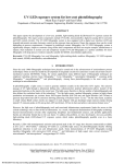
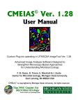
1 CMEIAS Color Segmentation
User Manual
Colin A. Gross, Chandan K. Reddy & Frank B. Dazzo
Center for Microbial Ecology
© Michigan State University 2010
2 Table of Contents I. CMEIAS Color Segmentation License Agreement. . . . . . . . . . . . . . . . 5 II. Background Information . . . . . . . . . . . . . . . . . . . . . . . . 6 III. General Color Segmentation Protocol. . . . . . . . . . . . . . . . . . . 8 IV. Menu Structure . . . . . . . . . . . . . . . . . . . . . . . . . . . . . . 11 A. Overview . . . . . . . . . . . . . . . . . . . . . . . . . . . . . . . 11 B. Menu Options . . . . . . . . . . . . . . . . . . . . . . . . . . . . .12 1. File. . . . . . . . . . . . . . . . . . . . . . . . . . . . . . . . .12 a. Open . . . . . . . . . . . . . . . . . . . . . . . . . . . . . .12 b. Save . . . . . . . . . . . . . . . . . . . . . . . . . . . . . .12 c. Save as . . . . . . . . . . . . . . . . . . . . . . . . . . . . .12 d. Duplicate the Active Image . . . . . . . . . . . . . . . . . . . .12 e. Close Active Image. . . . . . . . . . . . . . . . . . . . . . . . 13 f. Acquire Image. . . . . . . . . . . . . . . . . . . . . . . . . .13 1. Select Twain Source . . . . . . . . . . . . . . . . . . . . . 13 2. Acquire Twain Image . . . . . . . . . . . . . . . . . . . . 13 g. Print Preview – Active Image. . . . . . . . . . . . . . . . . . . 13 h. Print Setup. . . . . . . . . . . . . . . . . . . . . . . . . . . 13 i. Print Active Image . . . . . . . . . . . . . . . . . . . . . . . 13 j. Recent Files . . . . . . . . . . . . . . . . . . . . . . . . . . 13 k. Exit . . . . . . . . . . . . . . . . . . . . . . . . . . . . . . 13 2. Edit. . . . . . . . . . . . . . . . . . . . . . . . . . . . . . . . 14 a. Undo . . . . . . . . . . . . . . . . . . . . . . . . . . . . . 14 b. Redo . . . . . . . . . . . . . . . . . . . . . . . . . . . . . . 14 c. Copy . . . . . . . . . . . . . . . . . . . . . . . . . . . . . 14 d. Paste . . . . . . . . . . . . . . . . . . . . . . . . . . . . . 14 3. View . . . . . . . . . . . . . . . . . . . . . . . . . . . . . . . 14 a. Tool Bar . . . . . . . . . . . . . . . . . . . . . . . . . . . . 14 b. Status Bar . . . . . . . . . . . . . . . . . . . . . . . . . . . 14 c. Fit to Screen . . . . . . . . . . . . . . . . . . . . . . . . . . 15 3 d. Zoom In. . . . . . . . . . . . . . . . . . . . . . . . . . . . . . 15 e. Normal Viewing (1:1) . . . . . . . . . . . . . . . . . . . . . . . 15 f. Zoom Out. . . . . . . . . . . . . . . . . . . . . . . . . . . . . 15 g. Select Pixel Sampling Cursor . . . . . . . . . . . . . . . . . . . . . . 15 4. Process . . . . . . . . . . . . . . . . . . . . . . . . . . . . . . . . 16 a. Segmented Image Background. . . . . . . . . . . . . . . . . . . . 16 b. Color Similarity Tolerance. . . . . . . . . . . . . . . . . . . . . . 16 c. Apply Color Segmentation. . . . . . . . . . . . . . . . . . . . . . 18 d. Apply Color Dilation. . . . . . . . . . . . . . . . . . . . . . . . .18 e. Apply Color Erosion. . . . . . . . . . . . . . . . . . . . . . . . . 19 f. Fill Small Holes . . . . . . . . . . . . . . . . . . . . . . . . . . . 20 g. Color Models . . . . . . . . . . . . . . . . . . . . . . . . . . . . 20 1. Split to RGB Channels . . . . . . . . . . . . . . . . . . . . . . 20 2. Split to YUV Channels . . . . . . . . . . . . . . . . . . . . . . 21 3. Split to HSI Channels . . . . . . . . . . . . . . . . . . . . . . 22 4. Convert to Pseudocolors. . . . . . . . . . . . . . . . . . . . . 22 h. Flip Image . . . . . . . . . . . . . . . . . . . . . . . . . . . . . 23 1. Horizontal . . . . . . . . . . . . . . . . . . . . . . . . . . 23 2. Vertical . . . . . . . . . . . . . . . . . . . . . . . . . . . 23 i. Negative Image . . . . . . . . . . . . . . . . . . . . . . . . . . 23 j. Rotate Image Clockwise . . . . . . . . . . . . . . . . . . . . . . 23 k. Save Sampled Pixels . . . . . . . . . . . . . . . . . . . . . . . . 24 l. Load Sampled Pixels . . . . . . . . . . . . . . . . . . . . . . . .24 m. Discard Sampled Pixels . . . . . . . . . . . . . . . . . . . . . . .24 5. Filters . . . . . . . . . . . . . . . . . . . . . . . . . . . . . . . . . 24 a. Color‐to‐Grayscale . . . . . . . . . . . . . . . . . . . . . . . . .25 b. Brightness Threshold . . . . . . . . . . . . . . . . . . . . . . . .25 c. Adjust Hue/Saturation . . . . . . . . . . . . . . . . . . . . . . .26 d. Increase Intensity (+) . . . . . . . . . . . . . . . . . . . . . . . .26 e. Decrease Intensity (‐). . . . . . . . . . . . . . . . . . . . . . . . 26 f. Adjust Contrast. . . . . . . . . . . . . . . . . . . . . . . . . . .26 g. Min‐Max Object Size Filter . . . . . . . . . . . . . . . . . . . . . .27 h. Smoothen. . . . . . . . . . . . . . . . . . . . . . . . . . . . . .28 i. Sharpen Object Edges . . . . . . . . . . . . . . . . . . . . . . . 28 j. Find Object Edges . . . . . . . . . . . . . . . . . . . . . . . . . 28 k. Emboss. . . . . . . . . . . . . . . . . . . . . . . . . . . . . . 29 4 6. Window. . . . . . . . . . . . . . . . . . . . . . . . . . . . . . . . 30 a. Cascade . . . . . . . . . . . . . . . . . . . . . . . . . . . . . . 30 b. Tile. . . . . . . . . . . . . . . . . . . . . . . . . . . . . . . . 30 c. Close All . . . . . . . . . . . . . . . . . . . . . . . . . . . . . 30 d. Windows List . . . . . . . . . . . . . . . . . . . . . . . . . . . 30 7. Help. . . . . . . . . . . . . . . . . . . . . . . . . . . . . . . . . 30 a. About CMEIAS Color Segmentation . . . . . . . . . . . . . . . . 30 b. User Manual . . . . . . . . . . . . . . . . . . . . . . . . . . . 30 c. Help Topics . . . . . . . . . . . . . . . . . . . . . . . . . . . 30 d. CMEIAS Website . . . . . . . . . . . . . . . . . . . . . . . . . 31 V. References . . . . . . . . . . . . . . . . . . . . . . . . . . . . . . . . . 32 Appendix 1: Training Tutorial & Images . . . . . . . . . . . . . . . . . . . . 33 a. Apply these steps to each training image . . . . . . . . . . . . . 33 b. Segment the red fluorescent cells in Image1.tif . . . . . . . . . . . 34 c. Segment the Gram negative spiral bacteria in Image2.tif . . . . . . . 36 d. Segment the blue fluorescent cells stained with DAPI in Image3.tif . . 37 e. Segment the red, green and blue cells in Image4.tif . . . . . . . . . 39 f. Additional training not included in the AV tutorial. . . . . . . . . . 40 1. Segment the green fluorescent cells in Image1.tif . . . . . . . . 40 2. Segment the Gram positive rods in Image5.tif . . . . . . . . . . 41 5 I. CMEIAS© Color Segmentation Michigan State University Software License Agreement By downloading and installing a copy of this CMEIAS© Color Segmentation Software and Documentation, you agree to the following terms. Notification of Copyright: CMEIAS© Color Segmentation Software is a proprietary product of Michigan State University (“MSU”) and is protected by copyright laws and international treaty. You (as “End User”) must treat CMEIAS like any other copyrighted materials. Copyright laws prohibit making copies of the Software for any reason. You may make copies of the Documentation for use with a licensed version of the Software; however, MSU notifications of copyright must be left intact. If you have any questions concerning this agreement, please contact the Copyright Licensing Office, MSU, East Lansing, Michigan 48824 U.S.A. (517) 355‐2186 or (517) 432‐4499. License: MSU grants End User the royalty‐free, non‐exclusive, non‐transferable right to use CMEIAS Color Segmentation Software for research or educational purposes. You may not redistribute, transfer, rent, lease, sell, lend, sub‐license, prepare derivative works, decompile, or reverse‐engineer this CMEIAS© Color Segmentation Software without prior express written consent of MSU at the above address. MSU retains title to CMEIAS© Color Segmentation Software, including without limitation the Software and Documentation. End User agrees to use reasonable efforts to protect the Software and Documentation from unauthorized use, reproduction, distribution, or publication. All rights not specifically granted in this Agreement are reserved by MSU. Warranty: CMEIAS Color Segmentation Software and Documentation are provided “as is.” MSU MAKES NO WARRANTY, EXPRESS OR IMPLIED, TO END USER OR TO ANY OTHER PERSON OR ENTITY. SPECIFICALLY, MSU MAKES NO WARRANTY OF MERCHANTABILITY OR FITNESS FOR A PARTICULAR PURPOSE OF CMEIAS SOFTWARE OR DOCUMENTATION. MSU WILL NOT BE LIABLE FOR SPECIAL, INCIDENTAL, CONSEQUENTIAL, INDIRECT OR OTHER SIMILAR DAMAGES, EVEN IF MSU OR ITS EMPLOYEES HAVE BEEN ADVISED OF THE POSSIBILITY OF SUCH DAMAGES. IN NO EVENT WILL MSU LIABILITY FOR ANY DAMAGES TO END USER OR ANY PERSON EVER EXCEED THE FEE PAID FOR THE LICENSE TO USE THE SOFTWARE, REGARDLESS OF THE FORM OF THE CLAIM. General: If any provision of this Agreement is unlawful, void, or for any reason unenforceable, it shall be deemed severable from, and shall in no way affect the validity or enforceability of the remaining provisions of this Agreement. This Agreement shall be governed by Michigan law. 6 II. Background information: Microscopy and digital image analysis are important investigative tools in microbial ecology that provide direct quantitative information on the microbes’ world from their own perspective and spatial scale without the need for their laboratory cultivation. Unfortunately, much less information has been obtained from images of microbes than can actually be extracted using computer‐assisted microscopy, primarily because digital images of microorganisms in their natural habitats are highly complex, posing major challenges of image processing required for quantitative image analysis. An essential and most difficult task is object segmentation, which represents all editing steps required to reduce the image to the foreground microbial objects of interest before analysis. Complexity of image segmentation is increased even further when the organisms are colored to reveal important information on their ecological, biochemical, physiological, cytological and/or phylogenetic characteristics in situ (Fig. 1). As a consequence, information on the richness, abundance, metabolic activity and spatial heterogeneity of microbial populations and communities in complex environments is often visually described but rarely quantitated from true bitmap color images, compromising the potential impact of the study itself. 7 Figure 1. Hierarchical organization of various types of epifluorescence and transmitted light microscopy that utilize the discriminating power of color information to reveal significant characteristics of microorganisms. Abbreviations are: FISH, fluorescent in situ hybridization; CTC, (5‐cyano‐2,3‐ditolyl‐tetrazolium chloride); FITC, fluorescein isothiocyanate; Gfp, green fluorescent protein; DTAF, 5‐(4,6)‐dichlorotriazinyl‐aminofluorescein; DAPI, 4’,6‐diamidino‐
2‐phenylindole dihydrochloride. ELF™‐PO4 and SYTO™ BC are commercial trademarks. Image from Gross et al. 2009. 8 The challenge of color segmentation is how to separate foreground pixels from background along fine delineations of color and location within the complex image. The underlying problem is that microbial objects of interest in high definition, digital color images are commonly represented by pixels with heterogeneous brightness ranges of red, green and blue (RGB) that most often also include colored pixels of background at similar locations, and the pixels often have shallow gradients of brightness transition at cell borders resulting in indistinctive boundaries that contrast gradually with the background. This digital heterogeneity may not be noticeable when the image is viewed at 1:1 (100% zoom), but is obvious when magnified to view the color of individual pixels comprising the microbial objects (Fig. 2). Solving this challenging segmentation problem is crucial when any computer‐assisted microscopy application uses color information (Fig. 1) to extract ecologically relevant quantitative data, especially at the resolution and spatial scale of individual microbial cells and their ecological niches within environmental samples. Figure 2. Zoomed‐in detail of digital images showing variation in colored pixels comprising individual bacterial cells and the indistinct fluorescent halo surrounding their boundaries (due to the bending of light as it passes through the cell). The color stains and their corresponding RGB ranges within these cells are: (A) FITC r92‐r118, g198‐g255, b0; (B) DTAF r116‐r179, g166‐g246, b167‐b227; (C) crystal violet r62‐r157, g0, b167‐b227; (D) DAPI r1‐r74, g49‐g191, b157‐b255; (E) rhodamine r124‐r217, g0, b1‐b8. Bar scales equal 0.5 μm. Image from Gross et al. 2009. 9 Most often, color segmentation of microbial images is addressed by isolating the foreground object pixels with a single or narrow RGB color range, and/or splitting the color image into its individual RGB chromatic channels followed by thresholding the channel that contains the most intense signals for the targets of interest while suppressing the intensity of the other channels. This approach has variable degrees of success when applied to digitally pseudocolored monochrome images, such as those acquired as a primary grayscale image using confocal laser scanning microscopy and then pseudocolor processed for specific fluorochromes. Implementing other image processing routines such as dilation/erosion, Gaussian blur, contrast manipulation, spatial convolution masks, c‐means clustering, classification of pixels into predefined pseudochannel classes, mean‐median filtering, and measurement feature descriptors for object size and/or shape filtration can sometimes help to minimize blurred object edges and complement color channel‐based image segmentation of microbes. However, combinations of these image processing routines rarely succeed in segmenting the 3‐dimensional color space that accurately defines all foreground pixels of microbial targets of interest at all locations within complex, true bitmap color images to analyze their size, shape, abundance and spatial location in situ. In addition, underlying assumptions (e.g., RGB intensities of foreground object pixels are approximately equal to each other and greater than intensities of background objects) are not always valid, and the original true color intensities of the foreground objects are inevitably lost using these routines since they are typically applied to the whole image even when only selected areas require them. We sought to minimize these limitations by developing a more accurate, efficient, robust and versatile algorithm to semi‐automate the segmentation of multicolored microbes in digitized color images that also contain complex and usually noisy backgrounds, and to implement this improved technology into a well‐documented and user‐friendly PC software application. Earlier versions of our color segmentation algorithm are described in Reddy et al. 2003 and Reddy et al. 2004. In more recent work, we improved on the segmentation algorithm to achieve 99+% accuracy over a wider range of complex segmentation scenarios, and describe the computer vision logic of our new system, the accuracy of its significantly improved color segmentation algorithm, sources of error and how they are addressed, and examples of its application to solve various complex image processing challenges commonly encountered in color images acquired for quantitative microbial ecology studies (Gross et al. 2009). This free computing toolkit facilitates the integration of microbial ecology with cutting edge "individual single‐cell microbiology" at spatial scales directly relevant to the microorganisms themselves. This system is a component of CMEIAS© (Center for Microbial Ecology Image Analysis System) whose combined purpose is to strengthen microscopy‐
based approaches for understanding microbial ecology at μm spatial scales. III. General color segmentation protocol The CMEIAS Color Segmentation program segments RGB color images based on interactive sampling of pixels representing the RGB range for the foreground objects of interest, followed by mathematical computations of the color information weighted by a user‐defined threshold setting of their similarity in spatial distances. By including this 10 weighted similarity measurement, our system provides the flexibility to adapt to several different color groups for the segmentation process, even with complex backgrounds. The segmentation algorithm is then applied to produce the output image containing the segmented foreground objects of interest against a noise‐free pure black or pure white background. These functions all translate to a reduction in user's time and labor costs required to perform this essential image‐editing step, hence facilitating the whole process of digital image analysis. As with all applications of digital image analysis, the original color images of the microorganisms must be of high quality as a prerequisite. Figure 3. Flow of steps to segment the foreground objects in color images using the CMEIAS Color Segmentation software application. Image from Gross et al. 2009. 11 Figure 3 shows the general flow of steps used in this software application to segment foreground objects in color images with a complexity range typically encountered in microbial ecology studies. First, images are opened in the graphical user interface and examined to assess the similarity in color heterogeneity of the foreground objects and in their contrast to the background. Six different cursor designs have been included to optimize the precision of this pixel sampling process for a wide range of images. In addition, the RGB values of the pixel under the cursor automatically display in the status bar to assist with this initial evaluation. The information provided by this first step is used to set the color range tolerance on a scale that defines the range of color to be included in foreground pixels near each sampled pixel's location. Next, “training” pixels are interactively and carefully sampled from the objects of interest in each region of similar color within the active image. The required number of pixels sampled varies depending on their color heterogeneity within the foreground objects and how isolated are those regions within the image. Doing this pixel‐sampling task while viewing the cells in a zoom mode can be helpful. The time required will depend on the size and complexity of the image, number of sampled foreground pixels, and whether the signal and noise contents of the currently active image are sufficiently similar to previously segmented images whose array of sampled training pixels had been previously saved. Once these interactively trained inputs are registered, the color segmentation algorithm is activated to analyze the image, pixel‐by‐pixel, using the color and spatial ranges specified by the user‐selected training pixels and the specified threshold value that defines their 3‐
dimensional color space to determine which pixels are to be included as foreground objects. The run time to complete this automated algorithm depends on the size of the input image, number of training pixels sampled, and speed of the computer. This computing time is reported in milliseconds in the status bar, and typically takes less than 2 seconds using a PC with Pentium 4 and 3.00 GHz CPU to process images commonly included in microbial ecology studies. After the pixel classification is completed, the software automatically creates and displays a new color segmentation output image in which the pixels of foreground objects are retained in their original color and position, and the non‐foreground pixels are painted either black or white (at the discretion of the user) to optimally contrast the noise‐free background. Subsequent iterations of this sequence plus combinations of other image post‐processing features (Figs. 3 & 4) can be applied further to refine the results of the output image and produce the final image segmentation desired. 12 IV. Menu Structure A.
Overview Figure 4. The menu structure of CMEIAS Color Segmentation, including preprocessing and post‐processing functionalities added to compliment the color segmentation algorithm thereby enhancing the utility of the software application. Preprocessing features include options to work with a duplicate image while comparing processed steps to the original, split the image to its RGB, YUV, or HSI color channels, specify the color similarity tolerance threshold levels and output image background color, adjust image intensity/contrast, and find/smoothen/sharpen object edges. Post‐color segmentation functionalities include a user‐defined minimum‐maximum object size filter to discriminate the size range of foreground objects included in the output image, a feature to fill "small holes" of lost pixels completely enclosed within foreground objects, and a color dilate/erode feature to eliminate residual background noise in the output image and compensate for object segmentation with imperfect parameter settings. These features handle common remaining segmentation problems inherent in fluorescence micrographs, e.g., where the curvature of strongly fluorescent cells creates halos of similarly colored pixels and/or fluorescent cells have dark internal areas at lower sampling density. A useful option to save and retrieve the color range of selected training pixels is also featured 13 to add semi‐automation capability to the color segmentation routine when many image samples of the same community are being processed. The “Save and Load Sampled Pixels” features also provide a useful shortcut when rerunning the color segmentation process at different color threshold tolerances to optimize its crucial setting. When displayed, the fully segmented 24‐bit RGB output image or its 8‐bit grayscale image derivative can be copied to the Window's clipboard or saved directly as is. B. Menu Options Fig. 5. Title bar, main menu items, toolbar shortcut icons, and status bar of the CMEIAS Color Segmentation graphical user interface. 1. FILE a. Open Shortcut: Ctrl+O The Open command loads images to display at their 1:1 original size. TIF, BMP and PNG image file formats are supported. Multiple images can be opened to form a stack, but only the most recently opened image in the active window can be processed. The time (sec with 0.001 precision) required to open the image will display in the status bar. b. Save Shortcut: Ctrl+S The Save command saves the active image to its same filename. Images can be saved in any of the supported image formats. c. Save As... The Save As command saves the active image to a different filename and/or location. Images can be saved in any of the supported image formats. d. Duplicate the Active Image The Duplicate command creates a new window displaying a copy of the current active image. If an image stack is opened, only the active top image will be duplicated. Use this feature to compare the original image to processed images derived from it. 14 e. Close Active Image The Close command closes the currently active image window. f. Acquire Image The Acquire Image command is used to acquire digital images using a TWAIN interface, e.g., digital camera, flatbed scanner. To use TWAIN, you must install the TWAIN driver provided by the device manufacturer and the appropriate Source Manager for the scanning device you are using. The Source Manager is a DLL file, available at http://www.twain.org/index.html. Note that there are separate versions for different Windows operating systems, so make sure that you install the correct one. This Acquire Image menu feature has 2 choices: 1. Select Twain Source... Use this command to select the external Twain‐compliant device to acquire images. When selected, a window will open allowing you to specify which Twain‐compliant device installed on your computer to use. 2. Acquire TWAIN Image When selected, the device driver and software for the external Twain‐compliant device that you have selected will be opened allowing you to acquire the image. g. Print Preview – Active Image This option displays the active image in a standard window before it is printed. h. Print Setup The Print Setup command presents the standard Windows printer setup dialog box used to select the printer, type of paper, orientation, printing quality, number of copies, and other information for future printing jobs. i. Print Active Image Shortcut: Ctrl+P The Print Active Image command prints the image in the active window. It supports any printer connected to your computer with the appropriate Windows‐compatible print driver installed. j. Recent Files The Recent Files menu feature lists the 9 most recently opened image files with their complete filename displayed for easily identification. A single click of any image file listed will open it into the program workspace. k. Exit The Exit command will terminate the CMEIAS Color Segmentation application. 15 2. EDIT a.
Undo Shortcut: Ctrl+Z The Undo command removes the last process or filter change made to the active image and restores it to the previous condition. Up to 8 iterations of the undo feature can be applied. b. Redo Shortcut: Ctrl+Y The Redo command re‐performs the last undo operation again on the active image. c.
Copy Shortcut: Ctrl+C The Copy command allows you to copy the active image to the Clipboard, where it can then be transferred to any Window’s compatible application that supports the “paste” command. You can also use this feature to transfer the active image to a graphics package for adding annotations (e.g., bar scale, image label, arrows, etc). d.
Paste Shortcut: Ctrl+V The Paste command displays the TIF, BMP or PNG image from the Clipboard into a new image window. One can save this pasted image under a new name and/or location. 3. VIEW a.
Tool Bar The Tool Bar feature displays the Toolbar below the main menu (Fig. 5) and contains shortcut icons for many common operations. When the mouse is positioned over an icon in the toolbar, the status bar at the bottom of the main window will immediately indicate what function that icon provides. When the cursor is held for a second over any icon, a tool tip indicating the action it performs will appear below the mouse cursor. b.
Status Bar The Status Bar at the bottom of the main graphical user interface window (Fig. 5) displays various information about the active image, including its zoom ratio, the x, y coordinates [0, 0 landmark origin in the upper left corner] and the RGB brightness intensities of the pixel located precisely at the cursor position, the number of pixels sampled to operate the color segmentation algorithm, the Time (s) [with millisecond precision] required to load the input image, its width x height pixel dimensions, and the number of bits required to store a single pixel (8 bits for grayscale, 24 bits for RGB). The brightness intensities will be independent values between 0‐255 for each RGB chromatic channel for color images, and be the same RGB values [0‐255] for grayscale images. 16 When a previously saved file of sampled pixels is loaded [see sections IV.B.4.k and IV.B.4.l], the number of pixels previously sampled in that saved file will display. If you select more pixels after loading the file of previously saved pixels, then this number will increment to include the newly sampled pixels. The status bar will also display the time [millisecond precision] required to run the color segmentation algorithm and display its resultant output image. When the cursor is positioned over a toolbar icon or menu item, the Status Bar displays context‐sensitive information about its function instead of the zoom / x, y coordinates / pixel brightness values. c. Fit to Screen The Fit to Screen command automatically changes the zoom level so that the active image can fully display within the graphical workplace on the monitor screen while maintaining its aspect ratio. Before using this option, you must maximize the image window. When this option is selected, the three other zoom options (described below) are inactive. d. Zoom In Shortcut: Ctrl++ The Zoom In command adjusts the zoom of the active image to a higher displayed magnification (ratios of 2:1, 4:1, 8:1 and 16:1). You can select to view the magnified area of the image by using the horizontal and vertical scroll bars. e. Normal Viewing (1:1) Shortcut: Ctrl+/ The Normal Viewing command returns the display of the active image to its 1:1 original size of view after previously being zoomed to a different size. This menu item is grayed out when the image is first loaded since it’s already at a 1:1 size (100% zoom). f. Zoom Out ­
Shortcut: Ctrl+ The Zoom Out command adjusts the zoom of the active image window to a lower displayed magnification (ratios of 1:2, 1:4, 1:8 and 1:16). g. Select Pixel Sampling Cursor This feature provides six different cursor choices to optimize the accuracy of the interactive pixel sampling process for a wide range of images. The default choice is the pointed tip of the Window’s standard arrow (far right example in the above image). 17 4. PROCESS a. Segmented Image Background This option allows the user to select a white (default) or black colored background for the color segmentation output image. Make that decision based on the type of microscopy used to acquire the image and type of object analysis to perform on the fully segmented image, e.g., black for epifluorescence, white for transmitted brightfield or phase contrast. b. Color Similarity Tolerance Figure 6. Dialog box displayed to specify the threshold setting that defines the color similarity tolerance for the color segmentation function. Process → Color Similarity Tolerance. This process adjusts the sensitivity of the color segmentation function. The color distance of this threshold setting represents the radii of all spheres (in 3D color space) of included colors whose center is the sampled pixel(s). A higher threshold value allows more distantly related colors to be included in the segmented image, while lower threshold values narrow the range of colors that will be included. The default value is arbitrarily set at 100. The dialog box that opens when this process is selected will accept color distance unit values from 1 to 400 (Fig. 6). Use of high color distance threshold values would aid color segmentation when the background and other colored pixels present in the image are significantly different from the foreground colored pixels of interest. Conversely, a low color distance threshold value would be used to more effectively segment images in which the RGB colors of interest are close in value to colors of background that need to be discarded. Figures 7A, 7B and 7C illustrate the color similarity tolerance function: Fig. 7A. Image segmentations applied to a red region of a color spectrum with Color Tolerance Limit set at 65, 100, and then 150. Note how an increase in color similarity tolerance setting allows a greater deviation in color from the sampled pixel to be included in the output image. 18 Figs. 7B­7C. Use of the color similarity tolerance feature to achieve accurate color segmentation on images whose background pixels are of similar color but differ in intensity. Black arrows pointing to the right show the progression of image processing iterations applied at lower similarity tolerance levels to achieve final segmentation. (Image from Gross et al. 2009). In (B), 2 cells in an anaerobic bioreactor community are stained by fluorescence in situ hybridization (FISH) using a 16S rRNA phylogenetic probe for Clostridium sp. This image was very noisy, containing foreground pixels afloat in a background of similarly colored pixels having a different intensity pattern typical of random static interference. Accurate color segmentation was achieved by initially setting a high color tolerance threshold level that included all the foreground pixels, and then gradually excluding background pixels from the result image by subsequent iterations of the color segmentation routine at progressively lower tolerance levels. In (C), autofluorescent pigments allow detection of cyanobacteria in an estuary sample. The accurate, desired result was achieved by selecting two training pixels (yellow arrows) from the colored regions of foreground objects and then performing automated segmentation iterations at decreasing color tolerance threshold levels starting at 160, followed by 105, 85, and finally 75 to gradually delete background pixels of autofluorescent detritus and smoothen each cell’s contour. Also note how touching cells can be separated (green arrow, bottom middle) using crucial adjustments in color tolerance before applying color segmentation. 19 c. Apply Color Segmentation This is the most important function of this software. Objects of interest (e.g., bacteria) within color images will consist of pixels with widely varying RGB values (Fig. 2) and therefore it will be difficult or impossible to segment an image to contain just the foreground object pixels of interest based on sampling a single pixel value. CMEIAS Color Segmentation applies a nearest neighbor approach to classify all the pixels within the active image and isolate those foreground pixels of interest based on the representative range of RGB values and their spatial proximity to the training pixels sampled. Once completed, the active image is converted into the color segmented output image with foreground objects in a noise‐free, user‐specified black or white background (Fig. 8). Before activating this tool, some pixels must be sampled (click the mouse left button to sample the pixel under the cursor; maxim um of 200) on the image that will approximate the RGB range of foreground objects of interest (e.g., bacteria). Status messages display when 190 and 200 pixels have been sampled. See Gross et al. (2009) for full documentation of the computer vision logic of this color segmentation algorithm in our new system, measurements of its accuracy (99+%) when tested on ground truth data from a wide variety of color images of microbial populations and communities, sources of error and how they are addressed, and examples of its application to solve various complex image processing challenges commonly encountered in color images acquired for quantitative microbial ecology studies. This algorithm’s run time depends on the image size, heterogeneity of color pixels, number of training pixels sampled, and speed of the computer. The time (with millisecond precision) required to complete the segmentation algorithm and produce the color segmented output image is displayed in the status bar. Figure 8. Original (A) and color segmented output images of the red (B) and green (C) fluorescent bacteria. In this example, the segmented image background was set as black. d. Apply Color Dilation This command applies a dilation filter to the active color segmented image, resulting in a slight enlargement of the foreground objects [background size diminishes]. This filter operates by converting all background pixels that have at least 1 foreground pixel neighbor to the average foreground color. It can be applied to RGB or grayscale images. This and the Color Erosion filter are mainly applied to correct certain types of errors in the color segmented output image made by the Apply Color Segmentation routine. For example, use the color dilation filter to regain foreground object pixels in the image when they have been erroneously deleted (called a “false dismissal” error) during color segmentation (Fig. 9). 20 Figure 9. An insufficient number of training pixels were sampled from the original image (A), resulting in the color segmented output image containing several erroneously excluded foreground pixels (B), which were efficiently added back by applying the color dilation filter (C). e. Apply Color Erosion The option applies an erosion filter to the active color segmented image, resulting in a slight reduction in size of the foreground objects [background size increases]. This filter operates by converting foreground pixels that have at least 1 background pixel neighbor to the background color. It can be applied to RGB or grayscale images. This and the Color Dilation filter are mainly applied to correct certain types of errors in the color segmented output image made by the Apply Color Segmentation routine. For example, use the color erosion filter to eliminate single isolated pixels representing background noise erroneously included as foreground in the color segmentation output image, and background pixels classified as foreground at the edge of an object (called a “false alarm” error) during color segmentation (Fig. 10). Figure 10. An insufficient number of training pixels were sampled from the original image (A), resulting in the color segmented output image containing several erroneously included background pixels (B, red arrows), which were efficiently removed by applying the color erosion filter (C). Caution: Use these Dilation and Erosion operations carefully and conservatively. Applying Color Dilation will merge very close objects together into one object and Color Erosion will NOT remove all of the added dilated pixels. 21 f. Fill Small Holes Occasionally, under‐sampling of foreground object pixels in the original color image may produce a color segmented output image containing pixels of background color completely enclosed within some foreground objects. The “Fill Small Holes” post‐
processing feature is provided to correct this type of false dismissal error. It automatically converts internal foreground pixels lost during color segmentation into the object’s average color. The program must have in memory the RGB value of at least one sampled foreground pixel in order to compute the mathematical morphology algorithm to perform this image processing task, so before applying this feature to fill holes with a new batch of images, you must first select at least one foreground object pixel. To access this routine, select Process → Fill Small Holes, and then specify the upper size limit of the holes to fill. An example of its use is illustrated in Fig. 11, where holes of different size within an object were filled using the hole size settings specified in pixels. Objects holes in grayscale images can also be filled using this feature after the color segmentation routine has been applied. Fig. 11. Sequential use of the Fill Small Holes post‐processing feature to convert internal foreground pixels lost during color segmentation into the object’s average color. Arrows point to the position where holes were filled by applying the filter at the indicated maximum hole size (pixels) setting. g. Color Models 1. Split to RGB Channels This feature will split the active image into three new, separate windows indicating the Red, Blue and Green chromatic channels (Fig. 12). In some cases, changing a color image into a single channel can facilitate its segmentation of the objects of interest, but more commonly, the objects contain colored pixels with two or three channels (Fig. 12). This feature helps to diagnose complex segmentation problems in color images. The recommended solution is to use the Apply Color Segmentation routine featured in this software. Applying this feature to a grayscale image will display its 3 RGB channels of equal brightness. 22 Fig. 12. Splitting of an RGB image into its Red, Green and Blue chromatic channels. 2. Split to YUV Channels This feature splits the active RGB image based on its YUV content. This is a color‐encoding scheme for natural pictures in which luminance and chrominance are separate. The human eye is less sensitive to color variations than to intensity variations. YUV allows the encoding of luminance (Y) information at full bandwidth and chrominance (UV) information at reduced bandwidth. The Y channel image is a color‐to‐grayscale conversion. The U channel maximizes the contrast between dark green cells and bright blue cells against the gray background, and the V channel maximizes the contrast between bright red cells and dark green cells against the gray background (Fig. 13). Such changes in contrast can be used in conjunction with brightness thresholding procedures to segment the colored cells. The Appendix I training tutorial includes the use of this feature to achieve color segmentation. Fig. 13. Splitting of an RGB image into its Y, U and V channels. The Y channel image is a grayscale conversion from the original image. The U and V channels have contrast adjustments that increase differences in luminosity between the blue and green cells and between red and green cells, respectively. 23 3. Split to HSI Channels Fig. 14. Vectors of the RGB color wheel. A. Saturation. B. Hue. C. Brightness. D. All hues. Source: Adobe Photoshop Help Center. Based on the human perception of color, the HSI model describes three fundamental characteristics of color (hue, saturation, brightness intensity) (Fig. 14): Hue is the color reflected from or transmitted through an object. It is measured as a location on the standard color wheel, expressed as a degree between 0° and 360°. The position at 12 o’clock is at 0° / 360°. In common use, hue is identified by the name of the color such as red, orange, or green. Saturation, sometimes called chroma, is the strength or purity of the color. Saturation represents the amount of gray in proportion to the hue, measured as a percentage from 0% (gray) to 100% (fully saturated). On the standard color wheel, saturation increases from the center to the edge. Intensity is the relative lightness or darkness of the color, usually measured as a percentage from 0% (black) to 100% (white). 4. Convert to Pseudocolors Fig. 15. Example of an RGB image converted to pseudocolors to enhance recognition of the object’s edge. In this example, cells have a fluorescent halo that obscures their surface. This option converts the active image into another with different colors that reflect the brightness intensity of the image pixels. The program does this by first converting the image to a grayscale and then assigns an RGB color for each increment of gray level brightness. This tool will work for both grayscale and RGB color images. This process can help to recognize the periphery of foreground objects when they are obscured (Fig. 15). 24 h.
Flip Image 1. Horizontal ­­ This tool flips the active image horizontally along its vertical axis. 2. Vertical ­­ This tool turns the active image upside down by flipping vertically along its horizontal axis. i. Negative Image The Negative Image command converts the brightness value of each pixel’s corresponding channel(s) in the original positive image to its inverse value in the 256‐step calibration to produce the negative output image (Fig. 16). For an RGB color image example, a pixel in the positive image with RGB values of [35, 203, 48] is changed to [220, 52, 207]. For a grayscale image example, a pixel in the positive image with a brightness value of 255 is changed to 0, and a pixel with a brightness value of 25 is changed to 230. This tool works on both RGB color and grayscale images (Fig. 16). Fig. 16. Inversion of the positive color and grayscale images using the Negative Image tool. j. Rotate Image Clockwise This option applies a clockwise rotation of the active image by a user‐defined angle. When selected, a dialog box displays to input any rotation value (in degrees) between 1 and 360 (default is 90) (Fig. 17). To increase the precision, the rotation angle can be specified with float values (with decimal points). This option is useful to make the image exactly horizontal when acquired from a twain device. Fig. 17. Applying the Rotate Image Clockwise feature to an image. 25 k. Save Sampled Pixels This time‐saving feature allows the set of digital information for the sampled pixels to be saved to a *.txt file for future use to facilitate the color segmentation of multiple images whose foreground objects have a similar or the same color range. The saved file has a tab‐
delineated format that allows ease of pasting into spreadsheets if so desired. When this option is chosen, a dialog box displays asking you to enter the text filename and location where the digital information for the set of sampled pixels will be saved. Only one set of sampled pixels exist while the program is running. When a user samples a pixel, its color and location are added to the set of sample pixels that can be resaved. Example of digital information saved in the text file of 3 pixels sampled from an image: 3Sample_Pixels.txt [user‐specified file name] X Y R G B 314 261 255 3 3 43 310 255 8 5 245 255 3 2 Load Sampled Pixels 196
l.
This time‐saving feature allows you to apply the color segmentation routine on an active image using the saved text file (see section IV.B.4.k above) containing the digital information on the set of pixels previously sampled from foreground objects with similar or the same RGB range in a different image. Once this option is chosen, a dialog box displays to specify the name and location of the saved text file from which the pertinent RGB range of training pixels is to be retrieved. This function will clear out any existing sampled pixels before loading the new set from the file. Additional sampled pixels can be added to the loaded pixel set and resaved. The color segmentation process will still work even if some of the coordinate locations of the loaded pixel set are beyond the bounds of the image to which the set is being applied. Nice CMEIAS shortcut tool ☺ ! m. Discard Sampled Pixels This command clears the current set of sampled pixels. Use this function frequently, for example, before sampling pixels for color segmentation of a new image! 5. FILTERS An image filter is a process that changes the shades and pixel colors of an image. Filters are used to increase brightness and contrast, and add various textures, tones and special effects to an image. 26 a. Color­to­Grayscale The Color­to­Grayscale filter converts the active 24‐bit RGB image into the corresponding 8‐bit grayscale image. Every pixel of the grayscale image has a brightness value ranging from 0 (black) to 255 (white), computed from the brightness values of its red (r), green (g) and blue (b) chromatic channels according to the following formula : (b*11 + g*59 + r*30)/100). As an example, Fig. 18 illustrates the color‐to‐grayscale conversion of fluorescent yellow‐
green bacterial cells to grayscale pixels with the corresponding brightness as foreground. Use this feature to convert final color segmented images to 8‐bit grayscale for CMEIAS semi‐automated object analysis and classification. Figure 18. Conversion of a 24‐bit RGB image to the corresponding 8‐bit grayscale image using the Color – to – Grayscale filter. This feature is also used to prepare images for quantitative CMEIAS image analysis of object luminosity. For example, to measure Gfp gene expression, the fluorescent image is first color segmented, then converted to the 8‐bit grayscale image, then inverted to produce the negative image, and finally quantitatively analyzed for grayscale brightness. In this way, the luminosity of the foreground objects is placed on a scale of 0‐255 that is proportional to the brightness intensity of Gfp gene expression (Gross et al. 2009). b. Brightness Threshold The Brightness Threshold tool converts a grayscale image to a binary image containing only pixels of pure black (0) and white (255), typically as a preface to further object analysis. When selected, it opens a dialog box to input a threshold value level (0 – 255). An automatic thresholding algorithm computes the default value. An “OK” response converts the active grayscale image to binary whereby its pixels with a brightness of less than the input value are converted into 0 (black), and pixels with brightness above the input value are converted into 255 (white). If the active image is a 24‐bit RGB, it is first converted to the corresponding grayscale image using the algorithm described in section 5a above, and then the grayscale image is automatically converted to the binary image by the threshold operation using the same specified brightness level. The Training Tutorial (Appendix I) illustrates the use of the brightness threshold together with the Split to YUV model to segment colored objects. 27 c. Adjust Hue/Saturation The hue, saturation and intensity characteristics of the RGB color wheel are described in Section IV.B.4.g.3 entitled “Split to HSI” and its accompanying Fig. 14. The Adjust Hue/Saturation filter allows the user to adjust the hue, saturation, and lightness of the entire active RGB image prior to selecting the foreground pixels of interest for color segmentation. When selected, it opens a dialog box with two inputs: one to enter the hue value and the other to enter the saturation value (Fig. 19). The default values are arbitrarily set at 12 and 50, respectively. An adjustment of the saturation level (purity of the color) represents a move across the radius of the color wheel (vector A), whereas an adjustment of the hue (= color) represents a move around its perimeter (vector B) (Fig. 19). Figure 19. Dialog box for the Adjust Hue / Saturation filter, and the color wheel showing the saturation (A) and hue (B) vectors. Use the Adjust Hue/Saturation filter option to add color to a grayscale image and convert it to RGB, or to make an RGB image look like a duotone by reducing its color values to one hue. Sometimes, this adjustment will facilitate the segmentation of foreground colors of interest in color segmentation. d. Increase Intensity + (plus) The Increase Intensity command increases the intensity of the image, i. e., increases the luminosity or brightness factor in the HSI model (Fig. 14 vector C). Each subsequent use of this option moves all of the pixels of the image closer to white (maximum lightness). This can be useful if background of an image is non‐homogeneous and already close to white. e. Decrease Intensity – (minus) The Decrease Intensity command decreases the intensity of the image, i. e., the brightness factor of the image is reduced. This filter is useful for processing images when all but just a few scattered pixels of the background are nearly black. In cases such as this, the background can be made completely dark. Be cautious when using this function as it may reduce the distinction of contrast between foreground and background objects. f. Add Contrast The Add Contrast filter makes simple adjustments to the tonal range of every pixel in the active image. Sometimes, this processing step can improve the subsequent sampling of pixels for color segmentation. This command does not work with individual channels and is not recommended for high‐end output, because it can result in a loss of detail in the image. 28 g. Min­Max Object Size Filter [Generate Preview & Optimize Size] [Apply Size Filter] This powerful MinMax Object Size Filter removes objects larger than the user‐defined, max size and smaller than the min size of foreground objects in the current image. It is typically used to remove non‐foreground pixels from an RGB color segmentation output image or an 8‐bit grayscale image after it has been thresholded to binary. Both submenu options of this filter [Generate Preview & Optimize Size, Apply Size Filter] require the user to define the size range of objects to be INCLUDED in the new image by indicating the minimum and maximum pixel areas for all objects considered as foreground. When applied, the filter paints a user‐defined background color to all pixels of objects whose size is outside the specified area range while retaining all pixels of foreground objects (at their input color) within that same size range (Fig. 20A‐E). Appling this filter to an image will not generate a new image, so it is advisable to use it with a duplicate rather than the original image. The Generate Preview submenu feature (Fig. 20B) is used to optimize the MinMax operation and recolor the image in accordance to what was inside and outside the given area bounds. In the new preview image generated, by default, orange color denotes objects that were outside the size range of the given area bounds, while a light blue color indicates the objects that were within the defined size bounds (Fig. 20C). Selecting the colored buttons labeled “Included Objects” and “Excluded Objects” (Fig. 20B) allows customization of the color scheme. Choose pure black and white for 8‐bit binary images. Fig. 20. Sequence of steps to use the Minimum/Maximum Object Size Filter to remove background noise from an image. A) Color segmented output image containing regular rod‐shaped foreground objects and background noise of small spheres and a large irregular shaped object of the same color. B) Dialog box displayed when “Generate Preview and Optimize Size” is selected. C) Preview output image displayed after applying the size filter to the input image. Steps B and C are repeated to optimize the size range of foreground objects. The settings have been optimized for this example, since the light blue foreground objects are discriminated from the orange objects of background noise whose size is outside the specified range. D) Dialog box to input the optimized size range when “Apply Size Filter to Image” is selected. E) Final output image with objects of background noise removed by this size filtration routine. 29 h. Smoothen This filter smoothens the jagged edges of foreground objects by softening the color transition between their edge pixels and background pixels. Since only the edge pixels of the foreground objects undergo change, no detail is lost. This filter is useful when cutting, copying, and pasting selections to create composite images. i. Sharpen Object Edges This filter applies a mild focus on foreground objects whose edge is somewhat blurred. Its sharpening algorithm operates by increasing the contrast of adjacent pixels only at the edges of foreground objects while preserving the overall smoothness of the image. j. Find Object Edges The Find Object Edges filter provides an interactive way to isolate a foreground object and erase its background and the inner regions. Pixels on the edge of the object lose their color components derived from the background, so they can blend with a new background. The primary purpose of this filter is to delineate the outline edges of objects as a precursor for other image processing tasks. For instance, it can be used to quickly visualize which foreground objects are at the edge of the objects of interest, and the extent that foreground objects are touching each other (Fig. 21). A second use is to produce a derivative image from which the foreground objects can be isolated, copied and pasted into other applications (Fig. 22 ABC). A third use is to help define the edges of cells of interest when a fluorescent halo extends from outside their contour into background (Fig. 23). The output image of this tool can be saved and used to reduce and/or eliminate the fluorescent halo around fluorescent cells in order to produce the final image for quantitative image analysis. Fig. 21. Use of the Find Object Edges filter to quickly find areas of the image where foreground objects are touching each other. Examples are indicated by white arrows. 30 Use of the Find Object Edges filter to isolate foreground objects for Figure 22abc. copying into another image. A) original multicolored image. B) color segmented output image of green cells. C) Output image of Find Object Edges filter applied to the green color segmented cells with separation of foreground and background pixels that can be further processed. k.
Figure 23. Use of the Find Object Edges filter to define the contour of cells with a fluorescent halo. Emboss This image‐processing feature produces a three‐dimensional textured perspective of foreground objects in the active image. It does so by brightening one side and darkening the opposite side (Fig. 24). This filter can reveal variations in pixel brightness of internal structures and provide perspective on object thickness and surface texture. Fig. 24. The Emboss filter is used to make tangential pseudo‐shadowcast output images from 24‐bit RGB (top) and 8‐bit grayscale (bottom) images. The angle of shadow is reversed in the rightmost inverted images using the Convert to Negative Image filter. 31 6. WINDOW a.
Cascade Cascading resizes and staggers layers of all the open image windows within the workspace below the main window so that each title bar is visible. b.
Tile Tiling resizes and arranges all the open image windows side‐by‐side in the workspace below the main window. c.
Close All This command closes all the windows that are opened in the main window. d.
Windows List This feature displays the list of images/windows that are present in the main window. The check mark denotes the active image. Any other window can be made active by just clicking on the corresponding image in the list. 7. HELP a.
About Cmeias Color Segmentation This command displays the About shield that also temporarily displays when launching the program (shown on the 1st page of this User Manual). This image provides information on the current version and authors of the CMEIAS Color Segmentation software, the CMEIAS homepage website url, copyright information, the CMEIAS logo and the desktop shortcut icon for this software. b. User Manual This command opens the CmeiasColorSegmentation.pdf file of this user manual document in your default program (e.g., Adobe Reader) assigned to display pdf files. The software installation places this file within the same folder as the executable CmeiasColorSegmentation.exe program file. c.
Help Topics This command displays the contents of the CMEIAS Color Segmentation help system. From its table of contents you can select the topic providing the information you need. Keywords can be entered from the Search tab to produce a list, which when selected will display the corresponding page with the keyword highlighted within the text. 32 d. CMEIAS Website This command opens the home page of the CMEIAS Project website in your computer’s default browser. The website url address is http://cme.msu.edu/cmeias. The Color Segmentation webpage can be accessed by clicking its Hot button displayed among other CMEIAS features on each webpage. Check it and the “CMEIAS News” page periodically for pertinent information, updates and new version releases. 8.
33 8. References Reddy, C. K., Feng‐I Liu and F. B. Dazzo. 2003. Semi‐automated segmentation of microbes in color images. In Color Imaging VIII: Processing, Hardcopy, and Applications. Proc. International Society for Electronic Imaging (SPIE)‐2003, R. Eschbach and G. Marcu (eds.), vol. 5008: 548‐559. DOI: 10.1117.12.472024 http://dx.doi.org/10.1117/12.472024 and http://spiedl.aip.org/getabs/servlet/GetabsServlet?prog=normal&id=PSISDG0050080000
01000548000001&idtype=cvips&gifs=yes&ref=no Reddy, C. K. and F.B. Dazzo. 2004 Computer‐assisted segmentation of bacteria in color micrographs. Microscopy & Analysis 18: 5‐7. (September, 2004 issue) Gross, Colin A., Chandan K. Reddy and Frank B. Dazzo. 2009. CMEIAS color segmentation: an improved computing technology to process color images for quantitative microbial ecology studies at single‐cell resolution. Microbial Ecology (online version: DOI 10.1007/s00248‐009‐9616‐7 ) Gross, Colin A., Chandan K. Reddy and Frank B. Dazzo. 2010. CMEIAS color segmentation: an improved computing technology to process color images for quantitative microbial ecology studies at single‐cell resolution. Microbial Ecology 59 (2): 400­414. Enjoy CMEIAS ! Frank Dazzo [email protected] 34 Appendix 1
Training Tutorial & Images
This appendix provides the text and the Before →After image illustrations for the CMEIAS Color Segmentation Training Demo (CmeiasColorSegmentation.wmv) distributed with the software. The audio­visual demo runs in Windows Media Player. a. To begin, apply the following same steps to each training image: 1. Start the program and maximize its workspace on your computer monitor. 2.
Opening the image (File → Open). 3.
Make a duplicate working copy of the image (File → Duplicate the Active Image). 4.
Close the original image (File → Close Active Image). 5.
Adjust the position and size of the copied image window so it fully displays at 1:1 zoom. 6.
Discard any sampled pixels in memory (Process → Discard Sampled Pixels). 7.
Evaluate the range of colors for the pixels of foreground cells by viewing their RGB values in the status bar as you move the cursor over the cells. 8. Follow the steps indicated below to segment the foreground bacteria of interest in the training images provided. 35 Before → After image. b. Segment the red fluorescent cells in Image1.tif: 1. Open Image1.tif. 2. Set the background color for the output image to black (Process → Segmented Image Background → Black) 3. While viewing the RGB values for pixels of red cells, note that they include intensities in both red and green chromatic channels, but no values of blue. 4. Set the Color Similarity Tolerance setting to 65 pixels (Process → Color Similarity Tolerance → 65 → OK). 5. Discard any sampled pixels in memory 6. Select 2 pixels from 2 red cells within the input image. 7. Apply the color segmentation function (Process → Apply Color Segmentation). 8. If necessary, apply 1 cycle of the erosion / dilation process (Process → Apply Color Dilation ); (Process → Apply Color Erosion ). 36 Before → After image.
1.
Segment the Gram negative spiral bacteria in Image2.tif: Open Image2.tif. 2.
Set the background color to white (Process → Segmented Image Background → White). 3.
Apply contrast (Filter → Apply Contrast). 4.
Set Color Similarity Tolerance to 100 pixels (Process → Color Similarity Tolerance → enter: 100 → OK). 5.
Discard any sampled pixels in memory 6.
Load previously saved set of RGB values for the sampled foreground pixels of the red cells (Process → Load Sampled Pixels → Select Image2pixels.txt → Open). 7.
Apply the color segmentation function (Process → Apply Color Segmentation). 8.
Note that background pixels within the same color range are included in the segmentation output image prepared using the above settings. These are derived from the red colored pixels of the halo surrounding the Gram positive bacteria in the same image. 9.
Optimize the MinMax Size Filter settings to remove the residual background pixels. First, select Filters → MinMax Object Size Filter → Generate Preview and Optimize Size → (accept default settings of 30 min / 1620 max) → OK. This will display a preview image with the foreground objects included within the specified size range colored as light blue and all other objects whose size lies outside the filter range colored as brownish orange (default color settings that the user can change). 10. In this case, the default settings of 30 pixels minimum to 1,620 pixels maximum work OK in discriminating the foreground objects (Gram negative spiral bacteria, colored aqua in the size filter preview image) from background noise of red pixel halos around the purple Gram positive rods, colored brownish orange in the size filter preview image. 11. After approving the optimized settings indicated by the preview image, apply the size filter to the color segmented output image again (Filters → MinMax Object Size Filter → Apply Size Filter to Image → (accept optimized settings) OK. 12. Voila! This procedure produces the final segmented output image with the red spiral bacteria accurately segmented in the noise‐free white background. 37 Before → After image.
c. Segment the blue fluorescent cells stained with DAPI in Image3.tif: 1. Open Image3.tif. The main challenge in segmenting this image is to fine‐tune the balance of color similarity tolerance so it adequately removes the noisy background while still including the very thin spirochetes as intact foreground objects. 2. Set the background color to white (Process→ Segmented Image Background → White). 3. Set the color tolerance level to 100 (Process→Color Similarity Tolerance→set at 100 → OK). 4. Discard any sampled pixels in memory 5. Sample 5‐7 pixels from cells near the borders around the entire image. Alternatively, load the previously saved set of RGB values for the sampled foreground pixels of the fluorescent bluish white Dapi‐stained cells for this image (Process → Load Sampled Pixels → Select Image3pixels.txt → Open). 6. Apply the color segmentation routine (Process→Apply Color Segmentation) 7. When using the Image3pixels.txt sampled pixel file, note that the upper left quadrat of the color segmented image output contains several cocci with internal holes painted with background white pixels. Fill those holes within these cells using the Fill Small Holes process with the default hole size setting of 20 pixels (Process → Fill Small Holes → OK). The color of the pixels used to perform this process is the average RGB value for the entire cell. 8. If necessary, apply the dilate / erode editing process to ensure that the pixels of the spirochete cells are continuous (Process→Apply Color Dilation; Process → Apply Color Erosion). Before → After image.
38 d.
1.
2.
3.
4.
5.
6.
7.
Segment the red, green and blue cells in Image4.tif: Open the Image4.tif training image. Make two duplicate images and close the original. Activate one duplicate image and apply the RGB color model to examine its complexity. (Process → Color Models → Split to RGB channels). The split images should look like the ones shown above. Note that the cells in the blue channel are segmented OK but the cells in the red and green channels have pixels of overlapping color and therefore are not well segmented. Activate a second duplicate image and apply the YUV color model (Process → Color Models → Split to YUV channels). The output images should look like the ones shown below (left to right: channels Y, U and V). Before → After image.
The Y channel image output is a grayscale equivalent of the original image. The image outputs of the U and V channels represent a transformation that discriminates the red, green and blue cells based on each group’s brightness level. Here we will illustrate how this discriminating luminosity can be used in conjunction with the Adjust Brightness Threshold tool to segment the 3 groups of cells. Make 2 duplicate images of the U channel image. They will be used to isolate the (originally blue) bright cells and the (originally green) dark cells from the U channel image. Next, position the mouse cursor over the bright cells [originally blue] in one of the duplicate U‐channel images and note the grayscale brightness values of its pixels in the status bar that range approximately between 200‐230. 39 8.
9.
Apply the Brightness Threshold filter at a setting level of 190 (Filter → Brightness Threshold → enter 190 → OK). Invert the brightness levels of this thresholded image using the Process → Convert to Negative Image function to produce the final segmented image containing only the original blue cells. The Before → After images display below. Before → After image.
10. Next we will isolate the green cells from the other duplicate U channel image. 11. Measure the brightness values of the darkest gray cells (originally green) by positioning the cursor over them and view their gray levels displayed in the status bar. The brightness values for the pixels of those cells range approximately between 33‐43. 12. Apply the Brightness Threshold filter using a setting level of 60 (Filter → Brightness Threshold → enter 60 → OK). 13. Remove any background pixels remaining in the output image using the erosion / dilation process. The before and after images are shown below. Before → After image.
14. Finally, we will isolate the red cells, which are the bright ones in the V channel image. To begin, duplicate the V channel image. 40 15. The bright cells (originally red) can be isolated from this image by applying the Brightness Threshold process using a setting level of 190 (Filter → Brightness Threshold → enter 190 → OK). 16. Convert the image to negative (Process → Convert to Negative Image), followed by one cycle of erosion / dilation to produce the final output image with the original red cells now fully segmented in a noise‐free white background. The before and after images are shown below. Now we will demonstrate a few other features of the software. 1. Open Image1.tif 2. Zoom in and Zoom out using the toolbar shortcut icons, or the keyboard shortcut hot buttons Control + and Control ‐. 3. Change the Cursor for pixel sampling (View → Select Pixel Sampling Cursor #4). 4. Flip the image horizontally (Process → Flip the Image → Horizonal) and vertically (Process → Flip the Image → Vertical). 5. Convert to Negative Image: (Process → Convert to Negative Image); (Filter → Color To Grayscale → Convert to Negative Image} 6. Rotate the image clockwise: (Process → Rotate Image Clockwise → Accept 90° default → OK). 7. Print functions: File → Print Preview Active Image → Close; File → Print Setup; File → Print (toolbar shortcut icon) 9. Help Menu: Display the About Shield (Help → About CMEIAS Color Segmentation); display the user manual (Help → User Manual) ; connect to the CCMEIAS website (Help → CMEIAS website), display Color Segmentation page, and also Contact Us page. 10. Thanks for watching this tutorial. Email me at [email protected] you have any questions. 41 Additional training not included in the CMEIAS Color Segmentation AV tutorial: I.
Segment the Green fluorescent cells in Image1.tif: 1.
Open Image1.tif. 2.
Set the background color for the output image to black (Process → Segmented Image Background → Black) 3.
While viewing the RGB values for pixels of green cells, note that they include intensities in both red and green chromatic channels, but no values of blue. 4.
Set the Color Similarity Tolerance setting to 65 pixels (Process → Color Similarity Tolerance → 65 → OK). 5.
Discard any sampled pixels in memory 6.
Select 2 pixels from 2 green cells within the input image. 7.
Apply the color segmentation function (Process → Apply Color Segmentation). 8.
If necessary, apply 1 cycle of the dilation / erosion process (Process → Apply Color Dilation ); (Process → Apply Color Erosion ). Before → After image.
42 II. Segment the Gram positive rods in Image5.tif: 1.
Open Image5.tif. This image poses several challenges for successful segmentation. Because of the very noisy background, a sufficiently large number of training pixels must be sampled from various Gram positive bacteria within the image. 153 sampled pixels of foreground objects are included in the Image4pixels.txt file. 2.
Zoom out to 1:2 ratio. 3.
Set the background color to white (Process→Segmented Image Background→White). 4.
Set the color tolerance level to 100 (Process→Color Similarity Tolerance→ set at 100 → OK). 5.
Discard any sampled pixels in memory 6.
Load the image5pixel.txt file of saved sampled pixels (Process→Load Sampled Pixels→ image5pixel.txt → OK). 7.
Apply the color segmentation routine (Process→Apply Color Segmentation). 8.
If necessary, fill small holes using the 20 pixel default setting. (Process → Fill Small Holes → 20 pixels → OK).