Download Page 1 On Two-Dimensional Indexability and Optimal Range

On Two-Dimensional Indexability and
Optimal Range Search Indexing
(Extended Abstract)
Lars Arge
Vasilis Samoladasy
Abstract
Jerey Scott Vitterz
1 Introduction
There has recently been much eort toward developing worst-case I/O-ecient external memory data structures for range searching in two dimensions [1, 2, 4, 8,
12, 13, 20, 26, 28, 29]. In their pioneering work, Kanellakis et al. [13] showed that the problem of indexing
in new data models (such as constraint, temporal, and
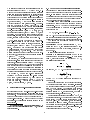
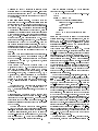
object models), can be reduced to special cases of twodimensional indexing. (Refer to Figure 1). In particular they identied the 3-sided range searching problem
(Figure 1(c)) to be of major importance.
In the rst part of this paper (Section 2), we apply
the theory of indexability [10] to two-dimensional range
searching problems. In indexability theory the focus is
on bounding the number of disk blocks containing the
answers to a query (access overhead ) given a bound on
the number of blocks used to store the data points (redundancy ). The search cost of computing which blocks
to access is ignored. We generalize the results in [26, 14]
and show a lower bound on redundancy for a given
access overhead for the general 4-sided problem. We
then show that this bound is tight by constructing an
indexing scheme with a matching tradeo between redundancy and access overhead. The indexing scheme
is based upon an indexing scheme for the 3-sided range
searching problem with constant redundancy and access
overhead.
In the second part of the paper, we develop optimal dynamic external data structures for 3-sided range
searching (Section 3) and 4-sided range searching (Section 4). (The update time is not provably optimal in
the 4-sided case.) Unlike in indexability theory, we
do not ignore the search cost when designing external
data structures. Our dynamic data structure for 3-sided
range searching is an optimal external version of the
priority search tree [16] based upon weight-balanced Btrees [2].
Throughout the paper we use capital letters to denote
parameter sizes in units of data points:
N = size of the data set;
B = disk block size;
T = size of the query output:
In this paper we settle several longstanding open problems in
theory of indexability and external orthogonal range searching. In the rst part of the paper, we apply the theory of
indexability to the problem of two-dimensional range searching. We show that the special case of 3-sided querying can
be solved with constant redundancy and access overhead.
From this, we derive indexing schemes for general 4-sided
range queries that exhibit an optimal tradeo between redundancy and access overhead.
In the second part of the paper, we develop dynamic external memory data structures for the two query
types. Our structure for 3-sided queries occupies O(N=B )
disk blocks, and it supports insertions and deletions
in O(logB N ) I/Os and queries in O(logB N + T =B )
I/Os, where B is the disk block size, N is the number of points, and T is the query output size. These
bounds are optimal. Our ,structure for general (4-sided)
range searching occupies O (N=B )(log(N=B ))= log logB N
disk blocks and answers queries in O(logB N + T =B)
I/Os,
which are optimal. It also
,
supports updates in
O (logB N )(log(N=B ))= log logB N I/Os.
Center for Geometric Computing, Department of Computer
Science, Duke University, Box 90129, Durham, NC 27708{0129.
Supported in part by the U.S. Army Research Oce through
MURI grant DAAH04{96{1{0013 and by the National Science
Foundation through ESS grant EIA{9870734. Part of this work
was done while visiting BRICS, Department of Computer Science,
University of Aarhus, Denmark. Email: [email protected].
y Department of Computer Sciences, University of Texas at
Austin, Austin, TX 78712-1188. Email [email protected]
z Center for Geometric Computing, Department of Computer
Science, Duke University, Box 90129, Durham, NC 27708{0129.
Supported in part by the U.S. Army Research Oce through
MURI grant DAAH04{96{1{0013 and by the National Science
Foundation through grants CCR{9522047 and EIA{9870734.
Part of this work was done while visiting BRICS, Department of Computer Science, University of Aarhus, Denmark and
I.N.R.I.A., Sophia Antipolis, France. Email: [email protected].
1
a
0110 10101010
0
1
0 1010101010
1
110
0
1
0
00
11
0
11
00
00 1
11
0
1
00
11
00
11
00
11
00
11
00
11
0
1
00
11
0011
11
00
11
0011
11
00
00
00
11
00
00 11
11
00
11
00
11
11
00
11
00
11
00
00
11
00
11
00
11
11 11
00
0011
00
c
b
a
a
(a) diagonal corner query at point a
0
1
0
1
0
0 1
1
0
1
0
1
0
1
0
1
0
1
0
1
0
1
01
1
01
0
1
01
1
0
0
0
1
0
0 1
01
1
0
11
0
1
0
1
0
0
1
0
1
0
1
1 1
0
0 1
0
a
(b) 2-sided query q = (a,b)
b
d
c
00
11
00
11
00
00 11
11
00
11
00
11
00
11
00
11
00
11
00
11
00
11
00
11
0011
11
00
11
0011
11
00
00
00
11
00
00 11
11
001
11
0
11
00
1
0
11
00
0
1
00
11
00
11
11 11
00
0011
00
(c) 3-sided query q = (a,b,c)
a
b
(d) 4-sided query q = (a,b,c,d)
Figure 1: Dierent types of two-dimensional range queries.
External range search data structures:
Background and outline of results
For notational simplicity, we dene
n= N
B
T
and t = B
to be the data set size and query output size in units of
blocks rather than points. An I/O operation (or simply
I/O) is dened as the transfer of a block of data between
internal and external memory.
Research on two-dimensional external range searching
has traditionally been concerned with the general 4sided problem. Many external data structures such as
grid les [17], various quad-trees [22, 23], z-orders [18]
and other space lling curves, k-d-B-trees [21], hBtrees [15], and various R-trees [9, 25] have been proposed. Often these structures are the data structures of
choice in applications, because they are relatively simple, require linear space, and in practice perform well
most of the time. However, they all have highly suboptimal worst-case performance, and although most are
dynamic structures, their performance deteriorates after repeated updates. The relevant literature is huge
and well-established, and is recently surveyed in [7].
Some progress has recently been made on the construction of external two-dimensional range searching
structures with provably good performance. The important subproblem of dynamic interval management is
considered in [13, 2]. A key component of the problem is
how to answer stabbing queries. Given a set of intervals,
a stabbing query with query point q asks for all the intervals that contain q. A stabbing query with query q is
equivalent to a diagonal corner query (a special case of
2-sided two-dimensional range searching ) in which the
corner of the query is located at (q; q) on the diagonal
line x = y. (See Figure 1(a).) Arge and Vitter [2] developed an optimal dynamic structure for the diagonal corner query problem. The structure uses O(n) disk blocks
to store N points, and supports queries and updates in
O(logB N + t) and O(logB N ) I/Os, respectively.
A number of elegant internal memory solutions exist for other special cases of two-dimensional range
searching. The priority search tree [16] for example
can be used to answer 3-sided range queries in optimal query and update time using linear space. A number of attempts have been made to externalize priority search trees, including [4, 12, 13, 20], but all
previous attempts have been nonoptimal. The structure in [12] uses optimal space, but answers queries
in O(log N + t) I/Os. The structure of [4] also uses
optimal space, but answers queries in O(logB N + T )
I/Os. In both these papers, a number of nonoptimal dynamic versions of the structures are developed.
Indexability: Background and outline of results
The theory of indexability was formalized by Hellerstein, Koutsoupias, and Papadimitriou [10]. As mentioned it studies an abstraction of an indexing problem
where search cost is omitted. An instance of a problem
is described by a workload W , which is a simple hypergraph (I; Q), where I is the set of instances, and Q is a
set of subsets of I . The elements of Q are called queries.
For a given workload W = (I; Q), and for a parameter
B 2 called the block size, we can construct an indexing scheme S as a B -regular hypergraph (I; B), where
each element of B is a B -subset of I , and is called a
block. We require that I = [B. An indexing scheme S
can be thought of as a placement of the instances of I
on disk pages, possibly with redundancy. It can thus be
seen as a solution to a data structure problem, assuming that searching for the appropriate blocks incurs no
cost.
An indexing scheme is qualied by two parameters:
its redundancy r and its access overhead A. The redundancy is a measure of space eciency and is dened as
r = B jBj=jI j. The access overhead A is dened as the
least number
such that every query q 2 Q is covered by
at most A jqj=B blocks of S , where jqj denotes the
number of points that satisfy query q. The reader is
referred to [10, 24] for a more detailed presentation.
Koutsoupias and Taylor [14] applied indexability to
two-dimensional range searching and showed that a particular workload, the Fibonacci workload, seems to be
worst-case for two-dimensional range queries. Using this
result, they showed logarithmic upper and lower bounds
on the redundancy for range search indexability.
In Section 2, we extend the previous results on the
Fibonacci workload by computing the exact worst-case
indexability trade-o between redundancy and access
overhead. We demonstrate that the lower bound is tight
by exhibiting a matching indexing scheme.
2
2.1 Lower bound for general range searching
The structure developed in [13] uses linear space but
answers queries in O(logB N + t + log B ) I/Os. Ramaswamy and Subramanian [20] developed a technique
called path caching for transforming an ecient internal
memory data structure into an I/O-ecient one. Use of
this technique on the priority search tree results in a
structure that can be used to answer 3-sided queries in
the, optimal O(logB N + t) I/Os but using nonoptimal
O n(log B ) log log B disk blocks
of space.
,
The structure can be updated in O (log N ) log B I/Os. Further modications led to the dynamic structure called
the p-range tree [26]. For 3-sided
queries, it uses linear
,
space, answers queries in O, logB N + t + IL (B ) I/Os,
and supports updates in O logB N +(logB N )2 =B I/Os
amortized. (The function IL is the very slowly growing
iterated log function, that is, the number of times that
the log function must be applied to get below 2.)
The p-range tree can be extended to answer general 4-sided queries in the same query bound using O(nlog, n) disk blocks of space; it supports
up
dates in O (log N )(logB N +(logB N )2 =B ) I/Os amortized. Ramaswamy and Subramanian also provide
a ,static structure with the same query bound using
O n(log n)= log logB N disk space. They prove for
a fairly general model that this space bound is optimal
that can answers queries in
, for any data structure
O (logB N )O(1) + t I/Os.
In Section 3, we present an optimal dynamic data
structure for 3-sided range searching that occupies O(n)
disk blocks, performs queries in O(logB N + t) I/Os, and
does updates in O(logB N ) I/Os. Part of the structure
uses the indexing scheme developed in the rst part of
the paper, and thus we demonstrate the suitability of
indexability as a tool in the design of data structures, in
addition to its application in the study of lower bounds.
In Section 4, we use our 3-sided structure to
construct a dynamic
structure for
4-sided queries
,
that uses O n(log n)=log logB N disk blocks of
space and answers queries in O(logB N + t) I/Os,
which
are optimal.1 Updates
,
can be performed in
O (logB N )(log n)= log logB N I/Os.
Samoladas and Miranker [24] developed a general technique for computing lower bounds for arbitrary workloads. In this section we combine their technique with
the results of [14] to obtain a lower bound on the tradeo between the redundancy r and the access overhead A
for the so-called Fibonacci workload.
We begin with a brief description of the Fibonacci
workload; we refer the reader to [14] for a thorough
presentation. Let N = fk be the kth Fibonacci number.
The Fibonacci lattice FN is the set of two-dimensional
points dened by:
FN = (i; ifk,1 mod N ) i = 0; 1; : : : ; n , 1 ;
for N = fk . The Fibonacci workload is dened by taking the Fibonacci lattice as the set of instances I , and Q
consists of queries in the form of orthogonal rectangles.
We will only use the following property of the Fibonacci lattice [14]:
Proposition 1 For the Fibonacci lattice FN of N
points and for ` 0, any rectangle with area `N contains between b`=c1c and d`=c2e points, where c1 1:9
and c2 0:45.
In [24] the following theorem is proved:
Theorem 1 (Redundancy Theorem) Let S be an
indexing scheme for queries q1 ; q2 ; : : : ; qM with access
ratio A, such that for every i in the range 1 i M ,
the following conditions hold:
jqi j B;
B ;
jqi \ qj j 2("A
)
for all j 6= i, 1 j M . The redundancy r satises
M
X
r " 2," 2 N1 jqi j;
i
where 2 < " < B=A is any real number such that B="A
2
=1
is an integer.
Let us apply this theorem to the Fibonacci workload.
The rst step is to design a set Q of queries. Intuitively,
we should consider queries of output size B , as these
seem to be the hardest. To be slightly more general,
however, we consider queries of size at least kB , for
arbitrary integer k 1. In this manner, we obtain a
more general result, depending upon k.
Our queries are rectangles of dimension ci a=ci , for
appropriate integers i. (The parameter c will be determined later.) The area of each rectangle is a, which
we set to c1 kBN . By Proposition 1, each such rectangle contains at least kB points. For each choice of i,
we partition the Fibonacci lattice into non-overlapping
rectangles of dimension ci a=ci , in a tiling fashion. All
these rectangles dene our query set Q.
2 Indexability of two-dimensional workloads
In this section we study the 3-sided and 4-sided range
searching problems within the indexability framework.
In Section 2.1 we provide a lower bound on the tradeo
between the redundancy r and the access overhead A
for the 4-sided problem. We show the bound to be tight
in Section 2.2 by designing an indexing scheme with the
same tradeo.
1 For notational simplicity, we use the expression log logB N to
denote the more complete expression log(logB N +1), whose value
is always at least 1.
3
Because no rectangle can have a side longer than N ,
we must constrain the integer i to satisfy ci N and
a=ci N , which puts i roughly in the range between
logc c1 kB and logc N ; that is, the rectangles have approximately logc (N=c1kB ) distinct aspect ratios. Since
we cover the whole set of points for each choice of i, it
follows from Theorem 1 that
!
N
log kB
"
,
2
N
r 2" logc c kB = log c :
1
In Section 2.2.1 we show how to construct an indexing
scheme for a 3-sided workload, with r = O(1) and A =
O(1). Interestingly, we were unable to achieve A = O(1)
for the case r = 1 in which there is no redundancy.
Whether this bound is possible is an interesting open
problem. In Section 2.2.2 we then consider general 4sided workloads.
2.2.1 Indexing schemes for 3-sided workloads
Consider a set of N points (xi ; yi ) in the plane ordered
in increasing order of their y-coordinates and let 2
be a constant. We describe a procedure to construct an
indexing scheme for the given points.
Initially, we create n disjoint blocks, b1 , b2, . . . , bn, by
partitioning the points based upon their x-order; that
is, for each i < j , if (x1 ; y1 ) 2 bi and (x2 ; y2 ) 2 bj , then
x1 x2 . We can associate an x-range with each block
in a natural way, along with a linear ordering of the
blocks. (If there are multiple blocks containing a single
x-value, any consistent linear ordering suces.)
We consider a hypothetical horizontal sweep line, initialized to y = ,1. We say that a block is active if it
contains at least one point above the sweep line. Initially all the blocks b1 , b2 , . . . , bn are active. We maintain the invariant that in each set of active blocks that
are consecutive in the linear ordering, at least one of the
blocks contains at least B= points above the sweep line.
We construct the other blocks for our indexing scheme
by repeating the following procedure: We raise the
sweep line until it hits a new point. If the invariant
is violated by consecutive active blocks, we form a
new block and ll it with the (at most B ) points that
are above the sweep line in the blocks. We mark the
blocks as inactive and make the new block active; it
replaces the blocks in the linear ordering. We do this
coalescing operation as many times as necessary until
the invariant is restored. The sweep line continues upwards until only one active block remains.
All the blocks constructed in this way form our indexing scheme. We start o with n active blocks and reduce
the number of active blocks by , 1 every time we coalesce blocks, so we create a total of at most n + n=( , 1)
blocks, which gives a redundancy of r 1 + 1=( , 1).
We can associate an active y-interval with each block
in a natural way: The active y-interval of block b is delimited by the y-coordinate of the point that caused b
to be made active (created) and the y-coordinate of the
point that caused b to become inactive.
To answer the 3-sided query q = (a; b; c), we consider
blocks whose active y-intervals include c, that is, the
blocks that were active when the sweep line was at y = c.
To cover the query, we look at the subset of these blocks
whose x-ranges intersect the interval [a; b]. This subset
is necessarily consecutive in the linear ordering. If there
are k such blocks, we know from the invariant that at
We determine parameter c using the second condition
of Theorem 1, which states that no two queries can intersect by more than B=2("A)2 points. We observe that
rectangles of the same aspect ratio do not intersect, and
rectangles of dierent aspect rations have intersections
of area at most a=c. From Proposition 1 it suces to
have
a=c B :
c2 N
2("A)2
Under the restriction that B 4("A)2 , the value
c = 4 cc1 k("A)2
2
satises the constraint. By choosing k = 1 we get the
following theorem:
Theorem 2 For the Fibonacci workload, the redundancy
and the access
overhead satisfy the tradeo r =
,
(log n)=log A .
More generally, we have the following theorem:
Theorem 3 For the Fibonacci workload, in order to
cover queries of T = tB points,with L + Adte blocks, the
redundancy must satisfy r = (log n)=(log L + log A) .
Proof : Since we have a weaker requirement on the query
cost, we only consider queries of size at least (L=A)B .
Smaller queries are not a problem, because each smaller
query is contained within a larger one. By setting k =
L=A in our analysis above, the theorem is proved. 2
If we set L = (logB N + 1)O(1) and A = O(1), we obtain the lower bound of [26]. For still higher values of L,
our lower bound on the required redundancy becomes
weaker.
2.2 Indexing schemes for two-dimensional
range searching
Proving the lower bound of the previous section to be
tight is not trivial. In [14], a method of deriving indexing schemes is given, but its redundancy exceeds the
optimal by a factor of B .2 In fact, in order to construct
optimal indexing schemes for 4-sided range-query workloads, we need to construct optimal indexing schemes
for 3-sided workloads.
2 Because of a slight error, the result as stated in [14] appears
to agree with our bound, but it is actually nonoptimal by a factor
of (B).
4
least b(k , 2)=c of them will contribute at least B=
points to the query output. Thus a query with output
size T satises T b(k , 2)=)c(B=), from which we
get k 2 t + + 1 and A 2 + + 1.
Theorem 4 For any 3-sided range searching workload
there exists an indexing scheme with r 1 + 1=( , 1)
and A 2 + + 1, for 2.
Choosing = 2 we get r 2 and A 7.
Corollary 1 For any 3-sided range searching workload
there exists an indexing scheme with redundancy O(1),
such that every query of size T is covered with at most
O(t + 1) blocks.
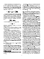
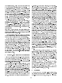
Figure 2: The solid lines represent the x-range of set
Si;j , covering query q shown as the dashed rectangle.
The vertical dashed lines represent the c-partition of
Si;j into Si,1;j , Si,1;j +1 , . . . , Si,1;j +c,1.
0
0
0
is not a leaf, its children partition q into k subqueries
q1 , q2 , . . . , qk , for some 2 k , as shown in Figure 2.
Subquery q1 is a 3-sided query with the unbounded side
to the right, and it can be covered by O(jq1 j=B + 1)
blocks of the appropriate child of Si;j . Similarly, subquery qk is a 3-sided query with the unbounded side
to the right, and it can be covered by O(jqk j=B + 1)
blocks of another child of Si;j . For each intermediate
subquery qj , for 1 < j < k, we can use either of the
indexing schemes for the appropriate child of Si;j to
cover qj in O(jqj j=B + 1) blocks. The total number of
blocks needed to cover query q is O( + jqj=B ).
Theorem 5 For any two-dimensional range searching
workload and any parameter 2, there, exists an in-
dexing scheme with redundancy r = O (log n)=log that covers every query of size T = tB with at most
O( + t) blocks.
2.2.2 Indexing schemes for 4-sided workloads
We now describe an algorithm by which we can create
an indexing scheme for any range query workload. Our
structure is based upon Chazelle's ltering technique [5].
We assume without loss of generality that N = k B ,
for some integers 2 and k 1. We rst partition
our data set of N points into L0 = N=B sets S0;j ,
for 1 j L0 , based upon their x-order. Each set S0;j
contains B points and ts into blocks. We say that
the sets form level 0 of our indexing scheme. Then we
create L1 = L0 = sets S1;j , for 1 j L1 , in which
each set S1;j is the distinct union of consecutive sets
of level 0. These sets form level 1. We continue this
process recursively, constructing the next level by unioning sets of the current level. We stop when we reach
level k , 1, for which Lk,1 = 1. Each set of level i contains i+1 B points; thus, there are L = N=i+1 B sets
at level i.
The sets Si;j constructed in the above way form a ary tree with k = log (N=B ) = log n levels, where each
non-leaf node is the union of its children. Each node of
this tree corresponds naturally to an x-range, and the
sets of each level form a partition of the data set.
We organize the points of every set Si;j into blocks, by
constructing two indexing schemes on the points of Si;j :
one that can answer 3-sided queries with the unbounded
side to the left, and one the can answer 3-sided queries
with the unbounded side to the right. (In the previous
section, the unbounded side was upwards). By the technique of the previous section, these indexing schemes
each occupy O(jSi;j j=B ) blocks and have access overhead O(1). Overall, we consume O(n) blocks per level,
and since we have log n levels, the redundancy is
3 Dynamic 3-sided range query data structure
We now turn to the problem of designing a linear space
external data structure for answering 3-sided queries.
After designing the indexing scheme for 3-sided queries
in Section 2.2.1, the only remaining issues are how to
eciently nd the O(t) blocks containing the answer to
a query and how to update the structure dynamically
during an insert or delete. The challenge is to do these
operations in O(logB N + t) I/Os and O(logB N ) I/Os,
respectively, in the worst case.
Our solution is an external memory version of a priority search tree [16]. In this structure we use a number of substructures derived from the indexing schemes
developed in Section 2.2.1, applied to sets of O(B 2 )
points each. In the next section we show how to make
our O(B 2 )-sized substructures dynamic with a worstcase optimal update I/O bound. The outer skeleton of
our external priority search tree is the so-called weightbalanced B-tree [2], which we review in Section 3.2. In
Section 3.3, we describe the external priority search tree
and show how to use the weight-balanced properties to
do updates in the worst-case optimal I/O bound.
n :
r = O log
log To answer a 4-sided query q = (a; b; c; d), we consider
the lowest node Si;j (the one with minimum i) whose xrange includes the query x-interval [a; b]. There are two
cases to consider. If Si;j is a leaf (i.e., at level i = 0), we
answer the query by loading the blocks of S0;j . If Si;j
5
3.1 Dynamic 3-sided queries on (B2) points
level (level 0), and rebalancing is done by splitting and
fusing internal nodes. However, they dier in the following important way: Constraints are imposed on the
weight of each node, rather than on its number of children. The weight of a leaf is dened as the number of
items in it; the weight of an internal node is dened
as the sum of the weights of its children. A leaf in a
weight-balanced B-tree with branching parameter a and
leaf parameter k (a > 4, k > 0) has weight between k
and 2k , 1, and an internal nodes on level ` (except for
the root) has weight between 21 a` k and 2a` k. A root
at level ` has weight at most 2a`k and has at least one
child. It can easily be shown that a weight-balanced tree
on N items has height loga (N=k) + (1) and that every internal node has between a=4 and 4a children. By
choosing a = (B ), we get a tree of height O(logB N );
when stored on disk, each internal node ts into O(1)
blocks, and a search can be performed in O(logB N )
I/Os.
In order to insert a new item into a weight-balanced
B-tree, we search down the tree to nd the leaf z in
which to do the update. We then insert the item into the
sorted list of items in z . If z now contains 2k items, we
split z into two leaves z 0 and z 00, each containing k items,
and we insert a reference to z 00 in parent (z ). After the
insertion of the new items, the weight constraint may
be violated at some of the nodes on the path from z
to the root; that is, the node v` on level ` may have
weight 2a`k. In order to rebalance the tree we split
all such heavy nodes, starting with the nodes on the
lowest level and working toward the root. The node v`
is split into v0̀ and v`00 such that they both have weight
approximately a`k. The following lemmas are proved
in [2]:
Lemma 2 After a split of a node v` on level ` into
two nodes v0̀ and v`00 , at least a` k=2 inserts have to pass
through v0̀ (or v`00 ) to make it split again. After a new
root r in a tree containing N items is created, at least
3N inserts have to be done before r splits again.
Lemma 3 A set of N = nB items can be stored in
a weight-balanced B-tree with parameters a = (B )
and k = O(B logB N ) using O(n) disk blocks, so that
a search or an insert can be performed in O(logB N )
I/Os. An insert perform O(logB N ) split operations.
We know from Corollary 1 that it is possible to build
an indexing scheme on O(B 2 ) points using O(B ) disk
blocks such that any 3-sided query can be covered by
O(t + 1) blocks. Because such an indexing scheme
contains only O(B ) blocks, we can store the activityinterval (y-interval) and x-range information for all the
blocks in O(1) \catalog" blocks. We can then answer a
query in O(t +1) I/Os simply by loading the O(1) catalog blocks into main memory and using the information
in them to determine which index blocks to access.
Given the O(B 2 ) points in sorted x-order a naive construction of the O(B ) blocks in the indexing scheme
using the sweep line process of Section 2.2.1 will require O(B 2 ) I/Os. However, the algorithm can be easily modied to use only O(B ) I/Os: When we create a
block (make it active), we determine the y-coordinate at
which point fewer than B=c of its points will be above
the sweep line, and we insert that y-value into a priority
queue. The priority queue is used during the sweep line
process to nd the next possible y-value where blocks
may need to be coalesced in order to restore the invariant. The total number of calls to the priority queue
is O(B ). Furthermore, the priority queue contains O(B )
entries at any time and can be kept in O(1) blocks in
internal memory. Thus only O(B ) I/Os are required to
construct the indexing scheme.
The above O(B ) construction algorithm can be used
to perform updates in O(1) I/Os per operation in the
worst case, by using the technique of global rebuilding [19]: We use two extra blocks, say, p and q, to log
insertions and deletions of points. When one of these
blocks becomes full, say, block p, we use block q to log
the next B updates, and at the same time we build a
new version of the structure out of the points in the current structure, updated as logged in p. The O(B ) I/Os
used to do the rebuilding can be spread evenly over the
O(B ) updates needed to ll block q, thus costing only
O(1) I/O per update. When the new version is complete, which will happen before block q has lled, we
switch to the new version of the data structure and we
swap the roles of p and q; we begin logging on block p
and building a new version using block q. Details will
appear in the full paper.
Lemma 1 A set of K B2 points can be stored in a
data structure using O(K=B ) blocks, so that a 3-sided
range query can be answered in O(t + 1) I/Os and an
update can be performed in O(1) I/Os worst case.
3.3 External priority search tree
An external priority search tree storing a set of N points
in the plane consists of a weight-balanced base tree built
upon the x-coordinates of the points, with parameters
a = B=4 and some k in the range B=2 k B logB N .
Each node therefore corresponds in a natural way to a
range of x-values, called its x-range.
Each node in the base tree has an associated auxiliary
data structure. Each of the N points is stored in the
3.2 Weight-balanced B-tree
Arge and Vitter [2] dened weight-balanced B-trees and
used them to construct optimal interval trees in external
memory. Weight-balanced B-trees are similar to normal B-trees [3, 6] (or rather B+ trees or more generally
(a; b)-tree [11]) in that all the leaves are on the same
6
for x = a and along the rightmost search path for x = b
are visited. Some nodes in the interior region between
the two search paths are also visited.
If z is a leaf node, visiting z involves accessing the
list Lz . If z 's x-range intersects one of the query's edges
x = a or x = b, the full list Lz must be traversed to
nd the relevant points. If instead the x-range of z lies
completely within the x-range of the query, it is possible
to access only the relevant part of the list, by taking
advantage of the fact that Lz contains points sorted on
the y-values.
Visiting an internal node v involves posing query q
to v's query structure Qv . After the relevant points
of Qv are reported, the search is advanced to some of
the children of v. (See Figure 4.) For each child w of v,
the search is advanced to visit w if one of the following
conditions holds:
auxiliary structure of exactly one node or leaf, according
to the following rules:
Each internal node v stores (at most) B points
in its auxiliary structure|at most B points corresponding to each of the (at most) B children of v.
For a child w of v, the set Y (w) of points contributed to v's auxiliary structure is called the Y-set
of w, by which we mean that the points in Y (w)
have the highest y-coordinates among the points
within the x-range of w that are not already stored
in ancestors of v. See Figure 3.
Each leaf stores (at most) 2k points in its auxiliary
data structure. The points stored in leaf z consist
of the points in z 's x-range that are not already
stored in ancestors of z .
If a node or leaf v has a non-empty auxiliary struc2
ture, then its Y-set (which it contributes to the
auxiliary structure of parent (v)) contains at least
B=2 points.
1. w is along the leftmost search path for x = a or the
rightmost search path for x = b, or
2. the entire Y-set Y (w) (stored in Qv ) satises the
query q.
We call the auxiliary data structure of an internal
node v its query data structure, and we denote it by Qv .
The query structure Qv contains all the Y-sets of v's
children|(B 2 ) points in total|and is implemented
to support 3-sided queries using the O(B )-block structure of Lemma 1. The auxiliary data structure of a leaf
node z consists simply of a list Lz (of blocks) sorted
according to their y-coordinates. Since each of the auxiliary structures uses linear space, the base tree occupies
O(n) blocks, and we get the following lemma:
Lemma 4 An external memory priority search tree
on N = nB points has height O(logB N ) and occupies
O(n) disk blocks.
The correctness of the recursive query procedure follows from the denition of the external priority search
tree. If the search procedure visits node v but not its
child w, that means that w is in the interior region and
at least one point p in Y (w) does not satisfy the query.
Since the x-range of w is completely contained in the
query's x-range [a; b], the point p must be below the
query's y-coordinate c. By denition of Y-set, all the
points in the subtree of w are no higher than p and thus
cannot satisfy the query.
We can show that a query is performed in the optimal
number of I/Os as follows: In every internal node v visited by the query procedure we spend O(1+ Tv =B ) I/Os,
where Tv is the number of points reported (Lemma 1).
There are O(logB N ) nodes visited on the direct search
paths in the tree to the leftmost leaf for a and the rightmost leaf for b, and thus the number of I/Os used in
these nodes adds up to O(logB N + t). Each remaining
internal node v that is visited is not on the search path,
but it is visited because (B ) points from its Y-set Y (v)
were reported when its parent was visited. If there are
fewer than B=2 points to report from Qv , we can charge
the O(1) I/O cost for visiting v to the (B ) points
of Y (v) reported from Qparent (v ). Thus the total I/O
charge for the internal nodes is O(logB N + t). A similar argument applies to the leaves: Only in two leaves
(namely, the ones for a and b) do we need to load all
O(B logB N ) points, which takes O(logB N ) I/Os. For
each remaining leaf z that we access, we use O(1+Tz =B )
I/Os. if Tz < B=2, we can charge the O(1) I/O cost to
the (B ) points in Y (z ) reported from Qparent (z) .
3.3.1 Optimal query performance
The basic procedure for answering a 3-sided query q =
(a; b; c) begins at the root r of the external priority
search tree and proceeds recursively to the appropriate
subtrees. All the nodes along the leftmost search path
v
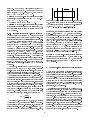
Figure 3: An internal node v of the base tree. For each
child w of v, the Y-set Y (w) consists of the (B ) highest points stored in the subtree of v that are within the
x-range of w. The Y-sets of the ve children of v are indicated by the bold points. They are stored collectively
in v in the query structure Qv .
7
v1
v2
v3
v4
v5
v1
v3
v2
(a)
v4
v5
(b)
Figure 4: Internal node v with children v1 , v2 , . . . , v5 . The Y-sets of each child, which are stored collectively in
the v's query structure Qv , are indicated by the bold points. (a) The 3-sided query is completely contained in the
x-range of v2 . The relevant points are reported from Qv , and the query is recursively answered in v2 . (b) The 3-sided
query spans several slabs. The relevant points are reported from Qv , and the query is recursively answered in v2 , v3 ,
and v5 . The query is not extended to v4 because not all of its Y-set Y (v4 ) (stored in Qv ) satises the query, and as
a result, none of the points stored in v4 's subtree can satisfy the query.
from the auxiliary structure of v0 into the auxiliary
structure of parent (v). In O(1) I/Os we nd the topmost point p0 stored in v0 by a (degenerate) query to the
query structure Qv . Then we delete p0 from Qv and insert it into Qparent (v) . This process may cause the Y-set
of one of the children of v0 to be too small (namely, the
Y-set that formerly contained p0 ), in which case we need
to promote a point recursively. The promotion of one
point may thus involve successive promotions of a point
from a node to its parent, along the path from v down
to a leaf. We call such a process a bubble-up operation.
The insertion of the x-coordinate of a new point p
is performed in the optimal O(logB N ) I/Os amortized:
According to Lemma 3, the initial insertion of x can be
performed in O(logB N ) I/Os and can cause O(logB N )
splits. Each split of an internal node v may cause B=2
bubble-up operations. By the above discussion and
Lemma 1, each bubble-up operation does O(1) I/Os at
each
, node on the path from v to a leaf, for a total of
O logB weight (,v) I/Os. Thus the
B=2 bubble-up operations use O B logB weight (v) I/Os. We also need
to split the auxiliary structure of v, which is straightforward for leaves and can be done for internal nodes in
O(B ) I/Os by Lemma
of ,node v can
, 1. In total a split
be performed in O B logB weight (v) = O weight (v)
I/Os. It then follows from Lemma 2 that each of the
O(logB N ) splits cost O(1) I/Os amortized.
After inserting x, the algorithm for inserting p involves traversing at most one root-to-leaf path in the
tree, querying and updating Qv at each node v on the
path, and a scan through the O(B logB N ) points in a
leaf. It follows from Lemma 1 that this insertion can be
performed in O(logB N ) I/Os.
Deletion of a point p = (x; y) is relatively straightforward. We recursively search down the path for the node
or leaf containing p. For each node v on the path, let vi
be the child whose x-range includes p. We use the query
structure Qv to identify the points in the Y-set Y (vi ).
If p is one of these points, we delete it from Y (vi ) (and
Lemma 5 Given an external memory priority search
tree on N = nB points, a 3-sided range query satised
by T = tB points can be answered in O(logB N + t)
I/Os.
0
3.3.2 Optimal updates|amortized
In order to insert a new point p = (x; y) into an external
priority search tree, we rst insert x into the base tree.
This may result in nodes in the base tree being split,
which may necessitate a reorganization of the auxiliary
structures. We defer the discussion of this reorganization temporarily. To insert the point p = (x; y) into
the appropriate query structure, we initialize node v to
be the root and do the following recursive procedure:
Let vi be the child of v whose x-range includes point p.
We identify the (at most) B points in the Y-set Y (vi ),
which are stored in v. These points can be identied
by performing the (degenerate) 3-sided query dened
by the x-range of vi and y = ,1 on the query structure Qv . If the number of such points is B=2 and p is
below all of them, then p is recursively inserted into vi .
Otherwise, p joins the Y-set Y (vi ) and is inserted into
v's query structure Qv . If as a result Y (vi ) contains
more than B points, the lowest of these points (which
can be identied by a query to Qv ) is deleted from Qv
(and thus Y (vi )) and is recursively inserted into vi . If
v is a leaf, then p is inserted into the correct position
in Lv . A simple scanning operation suces to nd the
proper location for p and to update the linear list. It
is easy to see that after the insertion the tree is a valid
external priority search tree.
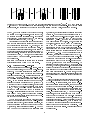
As mentioned above, auxiliary structures need to be
reorganized when a node v in the base tree splits into
nodes v0 and v00 . See Figure 5(a). After the split, one or
both of the Y-sets Y (v0 ) and Y (v00 ) obtained by splitting Y (v) may contain fewer than B=2 points. In the
worst case we need to promote the topmost B=2 points
from the auxiliary structure of v0 (resp., v00 ) into Y (v0 )
(resp., Y (v00 )). See Figure 5(b).
Let us consider the process of promoting one point
8
0
v
v1
v2
v3
v’
v4
v5
v1
v2
v’’
v3
v4
v5
(a)
(b)
Figure 5: Two views of a split. (a) Node v in the base tree splits into two nodes v0 and v00 . (b) When v splits, its
Y-set (shown by the bold points on the left) also splits, but in this case the two resulting Y-sets Y (v0 ) and Y (v00 )
are too small, and points need to be promoted from v0 and v00 into Y (v0 ) and Y (v00 ), as shown on the right.
,
thus Qv ), and if as a result Y (vi ) becomes too small,
we perform a bubble-up operation. If p is not in Y (vi ),
we continue the search recursively in vi . If the search
reaches a leaf z , we simply scan through Lz and delete p.
Overall p is deleted in O(logB N ) I/Os.
After deleting p we should also remove the endpoint x
from the base tree in order to guarantee that the height
of the structure remains O(logB N ). However, we can
aord to be lazy and leave x in the tree for a while. By
the principle of global rebuilding [19], we can leave x in
the tree and rebuild the structure completely after (N )
delete operations. It is easy to see that everything can
be rebuilt in O(N logB N ) I/Os, and so a delete costs a
total of O(logB N ) I/Os amortized. Details will appear
in the full paper.
Lemma 6 An update can be performed on an external
priority search tree in O(logB N ) I/Os amortized.
weight (v) subsequent insert operations has passed
through it. The purpose of the rebuilding phase on v
is to promote (via bubble-ups) the points needed for
constructing the Y-sets Y (v0 ) and Y (v00 ) and the query
structures Qv and Qv of the two new nodes v0 and v00
that will be created by the split. (We can determine
the points to promote for Y (v0 ) and Y (v00 ) before forming v0 and v00 by using a modied form of the 3-sided
structure used for Lemma 1.) During the process, we incrementally form the two new query structures, and we
incrementally insert the additional points for the two
Y-sets into Qparent (v) . When the rebuilding phase is
completed, the split can be nalized using O(1) I/Os.
One way of doing the rebuilding within worst-case
bounds is to decompose each bubble-up operation into
individual I/Os and to do the bubble-ups for v one I/O
at a time, doing one I/O each time v is accessed. An
insertion thus only takes O(logB N ) I/Os worst case.
However, by doing so, several bubble-up operations may
possibly be pending at a certain node, causing its query
data structure to be temporarily depleted until points
from below are percolated up. At such times, the data
structure will not be a valid external priority search tree
and queries will not be performed in the optimal number
of I/Os.
Below we discuss three approaches for scheduling the
bubble-up operations to obtain the optimal worst-case
I/O bounds. In all three cases, each time a root-toleaf path is visited during an insert, one or more of the
nodes on the path get complete bubbling-up procedures
done on them. Thus there will be no partially done
bubble-ups and the optimal query performance is retained. Each insert uses O(logB N ) I/Os on bubble-up
procedures, and it is guaranteed that when a node v
gets too heavy it will have B=2 bubble-up
, operations
performed on it (if necessary) within O weight (v)=B
operations that access v. After the necessary bubble up
operations have been performed, v can be split in O(1)
I/Os and we can thus guarantee that the split is accomplished before a new split needs to be initiated. This
proves one of our main results. (Details will appear in
the full paper).
0
3.3.3 Optimal updates|worst-case
The update algorithms in Section 3.3.2 are I/O-optimal
in the amortized sense, but have bad worst-case performance. The delete operations can easily be made
worst-case ecient using a standard lazy global rebuilding technique [19, 2]. Details will appear in the
full paper. However, obtaining a worst-case bound
on an insert operation is considerably more complicated. In the previous solution the number
of I/Os
,
required to perform an insert can be B (logB N )2 :
There can be (logB N ) splits per insert, and each split
may require (B ) bubble-up operations, each taking
(logB N ) I/Os. The tricky problem that remains in
order get a worst case bound is how to schedule the
bubble-up operations lazily so that each update only
uses O(logB N ) I/Os, while at the same time maintaining a valid external priority search tree so that the optimal query bound is retained.
The key idea we use to obtain the worst-case bound
is that when an internal node v in the weight-balanced
base tree gets too heavy, it is not split immediately, but
enters
a rebuilding
phase that extends over the next
,
O weight (v) insert operations accessing v. We know
from Lemma 2 that v will not have to split again until
9
00
Theorem 6 A set of N points can be stored in a data
After the insertion operation, we do the following
(complete) bubble-up procedures:
C := 0; fC counts I/Os done in bubble-up ops.g;
` := 1;
while C < 2 logB N do
if the node on level ` is eligible then
Perform a bubble-up operation for v
using ` I/Os;
C := C + `;
Reset v's count to 1;
structure using O(n) disk blocks, so that a 3-sided range
query can be answered in O(logB N + t) I/Os worst case,
and such that an update can be performed in O(logB N )
I/Os worst case.
Heavy leaf nodes method. Our rst method for
scheduling the bubble-up operations utilizes heavy leaf
nodes of size (B logB N ) rather than the normal (B ).
By Lemmas 4 and 5 this is allowable in an external priority search tree. Our algorithm is extremely simple.
We maintain a level counter ` for each leaf z , which is
initialized to 1 (corresponding to the level of z 's parent)
when z is created (split). Every time an item is inserted
into z , a bubble-up operation is performed on the node
at level ` above z , and ` is incremented by 1. When `
reaches the root level, it is reset to 1. Every insertion
is performed in O(logB N ) I/Os worst case. From the
time a leaf z is created until when it splits, (B logB N )
insertions are performed on z , and thus (B ) bubble-up
operations are performed on all the nodes on the path
to the root that are in a rebuilding phase when z is
created.
Lemma 7 Let v be an internal node in an external priority search tree. When v is in rebuilding mode, it will
get, (B ) bubble-up procedures
performed
on it within
,
weight (v)=B + B logB N = weight (v)=B insert
operations that visit v.
Proof
Sketch : The number
of leaves below v is
,
weight (v)=(B logB N ) . The worst case occurs when
each leaf is accessed enough times to do bubbleup operations for almost
all v's ancestors, but not
,
for, v itself. Thus
O
(log
N
B )weight (v )=(B logB N ) =
O weight (v)=B insert operations may be performed
below v without v having any bubble-up operations
performed. However, after this, on the average every
O(logB N ) insertions below v will cause a bubble-up
on v.
2
The proof of Lemma 7 remains valid if the leaf nodes
are of size maxfB; logB N g. We typically have B logB N , so for all practical purposes, the maximum is
equal to B .
Credit method. Our second method uses the same
general principle of doing complete bubble-up operations used in the heavy-leaf method. We show using a
credit argument how to allow the proper bubble-up operations and still keep the leaf nodes at the normal size
of (B ) points.
We give a count to each node in the weight-balanced
B-tree. The count is 0 when the node is not in rebuilding
mode, and it is nonnegative while in rebuilding mode.
During an insert operation, if the node v on level ` on
the root-to-leaf path is in rebuilding mode, then we increment v's count by 1. We say that v is eligible for a
bubble-up operation when its count is at least `.
endif
enddo
Lemma 8 Let v be a node on level ` 1 in the external
priority search tree. If v is in rebuilding mode, then for
any 1 b B , it will get b bubble-up
procedures
,
done
a
` := ` + 1; fWalk up one level in the treeg
on it within 4a`( a,+21 ) + 2b` = weight (v)=B insert
operations that visit v, where a = (B ) is the branching
parameter of the weight-balanced B-tree.
Proof Sketch : First consider the case b = 1. We will
show that v gets a bubble-up operation done on it within
4a`( aa+2
,1 )+ ` inserts that access it, assuming that it is in
rebuilding mode. The proof is by contradiction. Node v
becomes eligible for a bubble-up operation after ` insertion operations that visit it. Once v becomes eligible,
suppose that it does not receive a bubble-up operation
during the next 4a` ( aa+2
,1 ) accesses. It follows for each
of those insertions that there are always eligible nodes
below v on the insertion path (or else v would have received a bubble-up operation). Thus at least 2` worth
of I/Os for bubble-up procedures are done during each
insertion on v's descendants.
When v becomes eligible, the internal nodes below it
(which number at most 2a` + 4a`,1 + 4a`,2 + 4a`,3 +
+ 4a 2a` ( aa+2
,1 )) may be in rebuilding mode and
may be eligible too. Since each bubble-up operation
done on a node resets its count to 0, then after the
` a+2
4a`( aa+2
,1 ) inserts that visit v, at least 2a ( a,1 ) of the inserts do complete bubble-ups operations exclusively on
nodes that have already received complete bubble-ups
while v was eligible. Each insert operation may add 1 to
a node's count, which allows the node to do one future
I/O of work for a bubble-up procedure. Thus the total
added allowance to v's descendants per insertion is ` , 1
I/Os. On the other hand, at least 2` I/Os of bubble-ups
are done per insert while v is eligible. The 2a` ( aa+2
,1 ) inserts that do bubble-ups exclusively on nodes that have
received previous bubble-ups must therefore reduce the
nodes' allowances by at least 2a` ( aa,+21 )(2`) = 4a`( aa+2
,1 )`.
Since the allowances for those nodes are built up only
during v's eligible period, the allowances total at most
4a`( aa+2
,1 )(` , 1), and thus some of them must become
negative, which is impossible.
The argument for b > 1 is similar. After each bubbleup it receives, v needs to wait ` insertions before it be-
10
y-coordinate. For the fourth structure, we imagine linking together, for each child vi , for 1 i , the points
in the x-range of vi in y-order, producing a polygonal
line monotone with respect to the y-axis. We project
the segments produced in this way onto the y-axis and
comes eligible again, during which time its descendants
may accumulate a total allowance of ` per insert. 2
Child split method. Our third method uses generic
properties of B-trees to schedule the bubble-up operations. Let us consider a particular insertion. Let h be
the height of the tree, and let v0 ; v1 ; : : : ; vh be the nodes
of the path from the leaf where the new point is inserted
up to the root; that is, v0 is the leaf itself, and vh is the
root. We consider only the case where the leaf v0 splits,
but the root vh does not split. If this is not the case, no
bubble-ups are performed for this insertion.
By our assumption that the root does not split, we
conclude the there exists some k, for 0 < k h, such
that all the nodes v0 , . . . , vk,1 split, but none of the
nodes vk , . . . , vh split. In this case, node vk gets (up to)
bubble-up operations done on it. We call node vk the
designated node of this insertion. The following property is trivial:
Lemma 9 For any insertion where a leaf splits but the
root does not split, the number of children of the designated node increases by 1. All other nodes of the tree
either split or remain unchanged.
This proposition implies that the number of children
of a node increases as a result of an insertion if and only
if the node is the designated node of that insertion.
We now show that = O(1) is sucient to ensure
that every internal node vk will receive O(B ) bubbleups during its rebuilding phase. Let `1 be the number of
children that vk has when it enters its rebuilding phase
and let `2 be the number of children vk has when it is
ready to actually split. By Lemma 9, vk must be the
designated node for exactly `2 , `1 insertions during the
rebuilding phase. Thus, it receives (`2 , `1) bubbleup operations during rebuilding. Since `2 , `1 = (B ),
we can choose to be a suciently large constant to
guarantee that vk gets B bubble-up done on it in during
its rebuilding phase.
store them, together with all the segments produced in
the same way for the other siblings, in the linear space
external interval tree developed in [2]. Each point in the
x-range of v is thus stored in four linear-space auxiliary
data
, structures,so the auxiliary structures for v occupy
O weight (v)=B, disk blocks. Since
the tree has height
O(log n) = O (log n),=log logB N the whole
structure
occupies a total of O n(log n)= log logB N disk blocks.
To answer a 4-sided query q = (a; b; c; d), we use a
procedure similar in spirit to that of Section 2.2.2. We
rst nd the lowest node v in the base tree for which
the x-range of v completely contains the x-interval [a; b]
of the query. Consider the case where a lies in the xrange of vi and b lies in the x-range of vj . The query q
is naturally decomposed into three parts consisting of a
part in vi , a part in vj , and a part completely spanning
nodes vk , for i < k < j . The points contained in the
rst two parts can be found in O(logB N + t) I/Os using
the 3-sided structures corresponding to vi and vj . To
nd the points in the third part, we query the interval
tree associated with v with the y-value c. This gives us
the segments in the structure containing c, and thus
the bottommost point contained in the query for each
of the nodes vi+1 , vi+2 , . . . , vj,1 . We assume that each
segment in the interval tree for v has a link to a corresponding endpoint in the linear list of the appropriate
child of v. Following these links, we can traverse the
j , i , 1 sorted lists for vi+1 , vi+2 , . . . , vj,1 and output
the remaining points using O( + t) = O(logB N + t)
I/Os.
To do an update, we need to
, perform O(1) updates
on each of the O(log n) = O (log n)=log logB N levels of the tree. Each of these updates take O(logB N )
I/Os. We also need to update the base tree. If
we implement the base tree using a weight-balanced
B-tree and apply the techniques of Section 3.3, we
can
, show that the updates can be accomplished in
O (logB N )(log n)= log logB N I/Os. Additional details will appear in the full paper.
Theorem 7 A set of N =, nB points can be stored
in a data structure using O n(log n)= log logB N disk
blocks, so that a 4-sided range query satised by T =
tB points can be answered in O(logB N + t) I/Os
worst
case, and such that updates
can be performed in
,
O (logB N )(log n)= log logB N I/Os.
4 Dynamic 4-sided range query data structure
Using the optimal structure for 3-sided range searching
that we just developed, we show in this section how to
augment the approach in Section 2.2.2 with the appropriate search structures to obtain a optimal structure
for general 4-sided range queries.
Our structure for 4-sided queries consists of a base
tree with fan-out = logB N over the x-coordinates of
the N points. An x-range is associated with each node v
and this is subdivided by v's children v1 , v2 , . . . , v . We
store all the points that are in the x-range of v in four
auxiliary data structures associated with v. As in Section 2.2.2, two of the structures are for answering 3-sided
queries: one for answering queries with the opening to
the left and one for queries with the opening to the
right. We also store the points in a linear list sorted by
5 Conclusions
We have shown how to perform 3-sided planar (twodimensional) orthogonal range queries in I/O-optimal
worst-case bounds on query, update, and disk space
11
by means of an external version of the priority search
tree. Our approach can be extended to handle (general) 4-sided range queries with optimal query and space
bounds.
In practice, the amortized data structures we develop
or a modication of the static data structures that they
are based upon are likely to be most practical. It would
be interesting to compare our methods with other methods currently in use. Some initial work in that regard
is planned using the TPIE system [27].
There are several interesting range searching problems in external memory that remain open, such as
higher-dimensional range searching and non-orthogonal
queries. Some recent work has been done on I/Oecient three-dimensional range searching and halfspace range searching [1, 28, 29].
[14]
[15]
[16]
[17]
[18]
[19]
References
[20]
[1] P. K. Agarwal, L. Arge, J. Erickson, P. Franciosa, and
J. Vitter. Ecient searching with linear constraints.
In Proc. ACM Symp. Principles of Database Systems,
pages 169{178, 1998.
[2] L. Arge and J. S. Vitter. Optimal dynamic interval
management in external memory. In Proc. IEEE Symp.
on Foundations of Comp. Sci., pages 560{569, 1996.
[3] R. Bayer and E. McCreight. Organization and maintenance of large ordered indexes. Acta Informatica, 1:173{
189, 1972.
[4] G. Blankenagel and R. H. Guting. XP-trees|External
priority search trees. Technical report, FernUniversitat
Hagen, Informatik-Bericht Nr. 92, 1990.
[5] B. Chazelle. Filtering search: a new approach to queryanswering. SIAM J. Comput., 15:703{724, 1986.
[6] D. Comer. The ubiquitous B-tree. ACM Computing
Surveys, 11(2):121{137, 1979.
[7] V. Gaede and O. Gunther. Multidimensional access
methods. Computing Surveys, 30(2):170{231, 1998.
[8] R. Grossi and G. F. Italiano. Ecient cross-tree for
external memory. In J. Abello and J. S. Vitter, editors, External Memory Algorithms and Visualization.
American Mathematical Society Press, 1999.
[9] A. Guttman. R-trees: A dynamic index structure for
spatial searching. In Proc. SIGMOD Intl. Conf. on
Management of Data, pages 47{57, 1985.
[10] J. M. Hellerstein, E. Koutsoupias, and C. H. Papadimitriou. On the analysis of indexing schemes. In Proc.
ACM Symp. Principles of Database Systems, pages
249{256, 1997.
[11] S. Huddleston and K. Mehlhorn. A new data structure
for representing sorted lists. Acta Informatica, 17:157{
184, 1982.
[12] C. Icking, R. Klein, and T. Ottmann. Priority search
trees in secondary memory. In Proc. Graph-Theoretic
Concepts in Computer Science, LNCS 314, pages 84{
93, 1987.
[13] P. C. Kanellakis, S. Ramaswamy, D. E. Vengro, and
J. S. Vitter. Indexing for data models with constraints
[21]
[22]
[23]
[24]
[25]
[26]
[27]
[28]
[29]
12
and classes. Journal of Computer and System Sciences,
52(3):589{612, 1996.
E. Koutsoupias and D. S. Taylor. Tight bounds for 2dimensional indexing schemes. In Proc. ACM Symp.
Principles of Database Systems, 1998.
D. Lomet and B. Salzberg. The hB-tree: A multiattribute indexing method with good guaranteed performance. ACM Transactions on Database Systems,
15(4):625{658, 1990.
E. McCreight. Priority search trees. SIAM Journal of
Computing, 14(2):257{276, 1985.
J. Nievergelt, H. Hinterberger, and K. Sevcik. The grid
le: An adaptable, symmetric multikey le structure.
ACM Transactions on Database Systems, 9(1):257{276,
1984.
J. Orenstein. Spatial query processing in an objectoriented database system. In Proc. ACM SIGMOD
Conf. on Management of Data, pages 326{336, 1986.
M. H. Overmars. The Design of Dynamic Data Structures. Springer-Verlag, LNCS 156, 1983.
S. Ramaswamy and S. Subramanian. Path caching:
A technique for optimal external searching. In Proc.
ACM Symp. Principles of Database Systems, pages 25{
35, 1994.
J. Robinson. The K-D-B tree: A search structure for
large multidimensional dynamic indexes. In Proc. ACM
SIGMOD Conf. on Management of Data, pages 10{18,
1984.
H. Samet. Applications of Spatial Data Structures:
Computer Graphics, Image Processing, and GIS. Addison Wesley, MA, 1989.
H. Samet. The Design and Analyses of Spatial Data
Structures. Addison Wesley, MA, 1989.
V. Samoladas and D. Miranker. A lower bound bound
theorem for indexing schemes and its application to
multidimensional range queries. In Proc. ACM Symp.
Principles of Database Systems, pages 44{51, 1998.
T. Sellis, N. Roussopoulos, and C. Faloutsos. The
R+-tree: A dynamic index for multi-dimensional objects. In Proc. IEEE International Conf. on Very Large
Databases, 1987.
S. Subramanian and S. Ramaswamy. The P-range tree:
A new data structure for range searching in secondary
memory. In Proc. ACM-SIAM Symp. on Discrete Algorithms, pages 378{387, 1995.
D. E. Vengro. TPIE User Manual and Reference.
Duke University, 1997. Available at
http://www.cs.duke.edu/TPIE/.
D. E. Vengro and J. S. Vitter. Ecient 3-d range
searching in external memory. In Proc. ACM Symp. on
Theory of Computation, pages 192{201, 1996.
J. S. Vitter. External memory algorithms and data
structures. In J. Abello and J. S. Vitter, editors, External Memory Algorithms and Visualization. American Mathematical Society Press, 1999. Available at
http://www.cs.duke.edu/~jsv/.