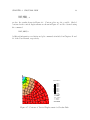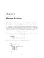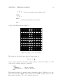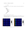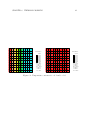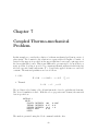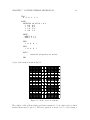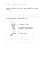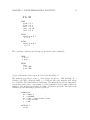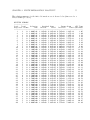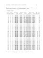
1
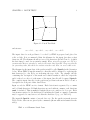
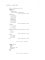
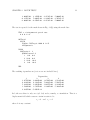
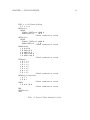
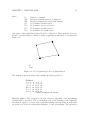
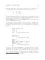
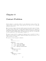
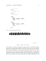
FEAP - - A Finite Element Analysis Program Version 8.4 Example Manual Robert L. Taylor Department of Civil and Environmental Engineering University of California at Berkeley Berkeley, California 94720-1710 E-Mail: [email protected] May 2013 Contents 1 Introduction 1 2 Patch tests 2 2.1 Plain Patch Test. . . . . . . . . . . . . . . . . . . . . . . . . . . . . . . 2 2.2 Axisymmetric patch test . . . . . . . . . . . . . . . . . . . . . . . . . . 7 2.2.1 Stability test . . . . . . . . . . . . . . . . . . . . . . . . . . . . 9 2.2.2 Consistency test . . . . . . . . . . . . . . . . . . . . . . . . . . . 12 3 Truss problem 15 4 Circular disk 18 5 Strip with hole and slit 30 6 Thermal Problem 37 7 Coupled Thermo-mechanical 42 8 Contact Problem 47 9 Finite Deformation Plasticity 51 i Chapter 1 Introduction In this manual we provide some examples of problems which can be set up and solved using the FEAP program. We begin by describing some of the methods which may be used to define an input data file for some simple finite element analyses. The manual is organized to start with very basic methods for inputs and precedes to more general methods to describe input data and problem solutions. FEAP is controlled using a set of commands. Each command performs a basic step in either describing a problem or solving a problem. Commands are divided into three basic groups: 1. Mesh description commands; 2. Problem solution commands; and 3. Graphical display commands. The appendices of the User Manual contain the optional forms which each input command may have. It is suggested that new users of FEAP carefully read this manual in its entirety before starting to generate their own input data. The later examples provide ways to manage the data for problems in separate files using an include option. Also, the form of the data input records may be constructed using parameters to which numerical values may be assigned either in numeric or expression form (see also Chapter 4 of the User Manual). 1 Chapter 2 Patch tests The first problems considered are simple patch tests in which all the data is specified explicitly. Later examples will illustrate how FEAP can add missing data or use repeating similar parts to generate a mesh. The patch test is a simple test which should be performed when first using any finite element program (see Chapter 11, Zienkiewicz and Taylor, 4th ed. Vol 1, for description of patch test). The patch test both ensures that the theory for the finite element formulation has been correctly implemented and that installation of the analysis system is also correct. 2.1 Plain Patch Test. For a plain strain or plane stress problem in linear elasticity one patch test is uniform stress in the x direction. This condition may be imposed on a square region divided into 4-elements and loaded by a constant x-traction on the right side as shown in Figure 2.1 (node 6 is located at y = 5 units). For a square with side lengths 10 and a 10 unit per length traction, the nodal forces on the boundary are 2.5 at the corners and 5.0 at the midside. The left side of the mesh is restrained so that no x-direction displacements occur and the lower left corner is also restrained in the y-direction. These restraints prevent rigid body motions as well as ensure that a correct solution to the constant stress problem may be obtained. For a linear elastic problem with the isotropic properties: Young’s modulus 1000 and Poisson ratio 0.25, the plane strain solution has displacements u = 0.009375 x ; v = − 0.003125 y 2 CHAPTER 2. PATCH TESTS 3 7 8 9 4 3 5 6 4 2 1 1 2 3 Figure 2.1: Patch Test Mesh and stresses σxx = 1.0 ; σyy = 0.0 ; σxy = 0.0 ; σzz = 0.25 The input data for each problem to be solved by FEAP is prepared and placed in a file on disk. It is recommended that the filename for the input data have a first character of I. The filename should not exceed 14 characters (12 in PC mode, of which the last 4 may be used for an extender .xxx). When using the program on a PC it is recommended that no extender be used for the main data input file. Feap uses this file for generating other files which do contain extenders and, thus, an error could occur. The filename for the input data of the patch test will be called Ipatch for the discussion below. When FEAP is run the names for other files will be assigned by replacing the first character (i.e., the I) by one indicating the type of file. For example, the file containing the description of the mesh and solution results is called the output file and for the above choice for the name of the input data file will be named Opatch. The complete input data file for the patch test problem is shown in Table 2.1 and a description for each part of this data follows. Input records for FEAP are free format. Each data item is separated by a comma and/or blank characters. If blank characters are used without commas, each data item must be included. That is multiple blank fields are not considered to be a zero. Each data item is restricted to 14 characters (15 including the blank or comma). Comments may be appended to any data record after the character ! (e.g., see Table 2.1). The input file Ipatch consists of several data sets. For the patch test mesh given in Table 2.1 the data sets are given by the commands (shown without indentation in the table): FEAP * * 4-Element Patch Test CHAPTER 2. PATCH TESTS FEAP * * 4-Element Patch Test 9,4,1,2,2,4 MATErial,1 SOLId PLANe STRAin ELAStic ISOTropic 1000.0 0.25 ! Blank termination COORdinates 1 0 0.0 0.0 2 0 4.0 0.0 3 0 10.0 0.0 4 0 0.0 4.5 5 0 5.5 5.5 6 0 10.0 5.0 7 0 0.0 10.0 8 0 4.2 10.0 9 0 10.0 10.0 ! Blank termination ELEMents 1 1 1 1 2 5 4 2 1 1 2 3 6 5 3 1 1 4 5 8 7 4 1 1 5 6 9 8 ! Blank termination BOUNdary restraints 1 0 1 1 4 0 1 0 7 0 1 0 ! Blank termination FORCes 3 0 2.5 0.0 6 0 5.0 0.0 9 0 2.5 0.0 ! Blank termination END 4 record record record record record Table 2.1: Data for Patch Test BATCh FORM residual TANGent SOLVe DISPlacement ALL STREss ALL END STOP Table 2.2: Data for Patch Test CHAPTER 2. PATCH TESTS 5 MATErial COORdinates ELEMents BOUNdary restraints FORCes END BATCh END STOP FEAP interprets only the first four characters of each command. These are shown as upper case letters to indicate the minimum amount which may be used to identify each command. Either upper case or lower case letters may be used to identify each command. Thus, MATE or mate may be used to identify the material property data sets. After a FEAP command and the control record, the commands before the first END may be in any order and define the mesh for the problem. The commands after the BATCH describe the solution algorithm for the problem and terminate with the second END command. Finally, the STOP command informs FEAP that no more data exists. Only one problem may appear in the file which contains the problem initiation command FEAP. See example in Chapter 5 for a way to run multiple problems. The control record defines the size of finite element problem to be solved. The first field defines the number of nodes (NUMNP), the next field is the number of elements (NUMEL), followed by the number of material sets (NUMMAT), the spatial dimension for the mesh (NDM), the number of degrees of freedom for each node (NDF), and the maximum number of nodes on any element (NEN). The patch test has a mesh with 9 nodes, 4 elements, and 1 material set. The problem is 2 dimensional, has 2 degrees of freedom at each node, and each element has 4 nodes. The first data set is identified by the MATErial command. This record also must contain a material set number (ranging from 1 to the maximum number of sets needed). The next records consist of commands which describe the type of element (see Chapter 6 of the User Manual for the types of elements included with FEAP) and the material parameters associated with the set. The data shown in Table 2.1 indicates a SOLId (continuum) element is used, the problem is plain strain and the material parameters are associated with a linear elastic isotropic material. Except for the element type record, other data may be in any order and terminates with a blank record (comments are permitted on records and begin with the exclamation point, ”!”). The values of the nodal coordinates for the patch are specified using the COORdinate command. Each record defines a node number, a generation parameter, and the x and y coordinate values. Nodes may be in any order, but are shown in increasing order in Table 2.1. Input terminates with a blank record. The manner in which nodes are connected to form individual finite elements and their CHAPTER 2. PATCH TESTS 6 association to the type of element and material parameters is described by the data following the ELEMent command. Each record defines the element number (which must be in increasing numerical order), a generation parameter (to be described later), the material data set associated with the element, and the list of nodes connected to the element. For the elements shown in Figure 2.1 the node sequence must start with a node at one vertex and then proceed with the nodes on vertices traversed counter clockwise around the element. Input terminates with a blank record. The degree of freedoms for each node may have known applied loads (nodal forces) or may be restrained to satisfy specified nodal displacements. In FEAP all degree of freedoms are assumed to have specified loading applied unless a restraint code is set. The BOUNdary restraint command may be used to assign restraints to degree of freedoms which are to have specified displacements. Each record defines a node number, a generation parameter, and the restraint codes for each degree of freedom associated with the node. A non-zero value for the restraint code indicates that the associated degree of freedom must satisfy a specified nodal displacement value (default is zero); whereas, a zero restraint code indicates the associated degree of freedom has a specified nodal force (also zero by default). Thus, for the data shown in Table 2.1, node 1 has both the u and v displacements restrained; nodes 4 and 7 have the u displacement restrained and the y force specified. All other nodes have both the x and the y forces specified since no restraints are specified. Input terminates with a blank record. It is evident from the remaining data that no data is provided to impose non-zero displacements (methods to input non-zero values are described in Section 5.7 of the User Manual); however, data is given to impose non-zero forces using the FORCe command. Each force record defines a node number, a generation parameter, and the force values for each degree of freedom associated with the node. Thus, for the data given in Table 2.1, nodes 3 and 9 have x force values of 2.5 units and node 6 has an x force value of 5.0 units. Input terminates with a blank record. The final command after the force values is the END command which terminates input of the data describing the finite element mesh. The set of commands shown in Table 2.2 define the solution algorithm to be used in solving the problem. The execution is initiated by the BATCh command (alternatively, it is possible to perform an interactive execution where users enter each command as needed, see next example and Chapter 11 of the User Manual). The FORM command instructs FEAP to form the residual for the equilibrium equations written as: R(u) = F − P(u) where F is the vector of applied nodal forces, u is the vector of nodal displacements, and for a static linear elastic problem P is defined as P = Ku in which K is the stiffness matrix. A solution to the problem is defined by requiring the residual to be zero. In FEAP the solution may be computed using Newton’s method CHAPTER 2. PATCH TESTS 7 which solves a sequence of linear problems. Thus, the TANGent command requests the tangent matrix to the residual about the current solution state, u (at start of execution the value is zero) where the tangent matrix is defined as: Ktang = − ∂R ∂u Thus, for a linear elastic static problem the tangent matrix is just K. The SOLVe command instructs FEAP to solve the incremental (Newton) equations Ktang ∆u = R and to update the solution as u ← u + ∆u For a linear problem this solution sequence should converge in one iteration; thus, the residual would be zero if the command FORM is given again. At this point FEAP has computed the solution; however, it is necessary to issue additional commands to output the values for each type of solution quantity. The DISPlacement command instructs FEAP to output values for the nodal generalized displacement parameters associated with each nodal degree of freedom (for linear elasticity using solid elements these are the values of the u and v displacements at a node). The option ALL requests the displacement values for all active nodes (see manual pages in Appendix A for other options). Similarly, the command STREss, ALL requests output values for stresses within all the active elements (see Appendix A for other options). All output is placed in the output file. 2.2 Axisymmetric patch test A three dimensional solid is described by a body of revolution and is to be analyzed for the case of axisymmetric behavior. Only small deformations are considered. For this case the displacement field is given by: ur (r, z) u= uz (r, z) (2.1) That is, the displacements do not depend on the θ coordinate; however, in FEAP all axisymmetric problems are formulated for a one radian sector in the θ direction and the factor 2 π is omitted. The stress and strain for an axisymmetric case may be ordered as: T σ = σrr σzz σθθ σrz (2.2) and T = rr zz θθ γrz (2.3) CHAPTER 2. PATCH TESTS 8 where γij = 2 ij . Using the displacements given by Eq. 2.1 the strain-displacement relations are given by (Reference: I.S. Sokolnikoff, Mathematical Theory of Elasticity, McGraw-Hill, New York, 1956, pp 182-184.) T ∂ur ∂uz ur ∂ur ∂uz = (2.4) , , , + ∂r ∂z r ∂z ∂r Similarly, for the above displacement field the equations of equilibrium are given by: ∂σrr ∂σrz σrr − σθθ + + + br = 0 ∂r ∂z r ∂σrz σrz ∂σzz + + + bz = 0 ∂r r ∂z (2.5) in which body forces also are axisymmetric and thus are given by b = b(r, z). For a displacement formulation, a variational problem for linear elasticity may be written as Z Z Z T T u t̄ r ds = min. (2.6) u b r dr dz − W () r dr dz − Π(u) = Ω Γt Ω where W is the stored energy function and ds is a differential length on the two dimensional r − z boundary. Note also that the factor 2 π is again not included for implementation into FEAP. Introducing an isoparametric interpolation for the finite element model as r z ur uz = = = = Nα (ξ) rα Nα (ξ) z α Nα (ξ) uαr Nα (ξ) uαz where ξ are natural coordinates, the strain-displacement relations become ∂Nα 0 ∂r α ∂N α 0 ur ∂z uαz = α N α 0 uθ r ∂N ∂N α ∂z α ∂r The variational problem generates the residual equation (again without the factor 2 π) Z Rα = Fα − BTα σ r dr dz Ω CHAPTER 2. PATCH TESTS 9 in which nodal forces are given by Z Z Fα = Nα b r dr dz + Ω Nα t̄ r ds Γt Linearizing generates the tangent stiffness used in solution of problems by a Newton method. Accordingly, after the linearization step we obtain Z BTα DT Bβ r dr dz Kαβ = Ω as the stiffness matrix in which DT is the matrix of tangent moduli for each material. The patch test satisfaction requires two parts: A stability test and a consistency test. Here the stability is assessed by computing the eigenvalues for a single element. 3 4 1 2 7 8 9 4 5 6 1 2 3 Figure 2.2: (a) 4-node element (b) 9-node element. 2.2.1 Stability test An eigenpair assessment is performed for the 4-node element shown in Fig. 2.2(a). The geometry and material properties are given by the commands: FEAP * * Axisymmetric patch test 0 0 0 2 2 4 MATErial SOLID ELAStic ISOTropic 1000.0 AXISymmetric BLOCk 0.25 CHAPTER 2. PATCH TESTS 10 CARTesian 1 1 QUADrilateral 4 1 0.0 0.0 2 10.0 0.0 3 10.0 10.0 4 0.0 10.0 END To compute the eigenvalues and eigenvectors the command language statements needed are: BATCh TANG,,-1 ! No factoring performed EIGE VECTor ! Eigenpair for last element END and results obtained are: Eigenvalue 1 1.0593E+04 3.5958E+03 1 2.9953E-01 1.3438E-01 -4.8127E-01 4.0076E-01 -4.8127E-01 -4.0076E-01 2.9953E-01 -1.3438E-01 2 1.0000E+04 1.6205E+03 3 6.1457E+03 9.2513E+02 4 4.4533E+03 1.8724E-12 Eigenvectors 2 3 6.3500E-01 -3.1106E-01 -1.2700E-01 -2.2639E-01 2.5400E-01 -5.4839E-01 -1.2700E-01 2.2639E-01 2.5400E-01 5.4839E-01 1.2700E-01 2.2639E-01 6.3500E-01 3.1106E-01 1.2700E-01 -2.2639E-01 4 4.5699E-02 -1.4460E-01 -4.4896E-01 -5.2482E-01 -4.4896E-01 5.2482E-01 4.5699E-02 1.4460E-01 Eigenvectors 5 6 7 8 6.2171E-01 7.0466E-02 1.2928E-01 6.2360E-17 -2.0666E-02 6.6701E-01 -4.4533E-01 5.0000E-01 -3.3559E-01 4.7990E-02 2.9436E-01 -1.1113E-16 2.0666E-02 -2.1870E-01 4.4533E-01 5.0000E-01 3.3559E-01 4.7990E-02 -2.9436E-01 -7.4079E-17 CHAPTER 2. PATCH TESTS 11 2.0666E-02 2.1870E-01 4.4533E-01 5.0000E-01 -6.2171E-01 7.0466E-02 -1.2928E-01 -1.7654E-17 -2.0666E-02 -6.6701E-01 -4.4533E-01 5.0000E-01 The test is repeated for the mesh shown in Fig. 2.2(b) using the mesh data: FEAP * * Axisymmetric patch test 0 0 0 2 2 9 MATErial SOLID ELAStic ISOTropic 1000.0 AXISymmetric 0.25 BLOCk CARTesian 2 2 QUADrilateral 9 1 0.0 0.0 2 10.0 0.0 3 10.0 10.0 4 0.0 10.0 END The resulting eigenvalues are (vectors are not included here) 1 3.8572E+04 9.8218E+03 5.2832E+03 1.5889E+03 4.9187E+02 Eigenvalue 2 3 3.0844E+04 1.6764E+04 9.3116E+03 7.8663E+03 3.6854E+03 3.0857E+03 1.5347E+03 1.1869E+03 -5.0762E-12 4 1.5316E+04 5.5895E+03 2.1230E+03 5.3488E+02 In both cases there is only one rigid body modes, namely, a z-translation. That is a displacement field which causes no strain is restricted to ur = 0 and uz = A where A is any constant. CHAPTER 2. PATCH TESTS 2.2.2 12 Consistency test The consistency test considers behavior under specified linear displacement fields that in general will have non-zero strains and stresses as well as non-zero body forces. For a part of the consistency test we consider the test applied to a displacement field expressed as: ur = A + B r and uz = 0 From this we obtain strains = B 0 A + B r 0 and for an isotropic material with constitution σij = λ εv δij + 2 µ ij where εv = ii is the volume change in small deformation, the stresses A λ + 2B + 2µB r A + 2B λ r σ= A A λ + 2 B + 2 µ + B r r 0 Inserting these stresses into the equilibrium equation requires a non-zero radial body force to be: A br = (λ + 2 µ) 2 r This body force distribution must be coded into each element to permit the testing of a patch performance. The isotropic elastic properties in feap are given in terms of Young’s modulus, E, and Poisson’s ratio, ν. From these we obtain E 2ν µ= and λ = µ 2 (1 + ν) (1 − 2 ν) which are used to compute the boundary tractions and body force br . For the example we let A = B = 1.0 The input data is given by: CHAPTER 2. PATCH TESTS 13 FEAP * * Axisymmetric patch test 0 0 0 2 2 9 PARAM mu = 1000/2.5 la = 0.5*mu t1 = (2.2*la + 2*mu)*5 t2 = (2.1*la + 2*mu)*5 br = la + 2*mu MATErial SOLID AXISymmetric ELAStic ISOTropic 1000.0 BODY PATCh br 0.25 0 BLOCk CARTesian 4 4 QUADrilateral 9 1 5.0 0.0 2 10.0 0.0 3 10.0 5.0 4 5.0 5.0 9 7.75 2.25 CSURf LINEAR 1 5 2 5 LINEAR 1 10 2 10 ! Tractions on radial boundary ! Note t1,t2 multiplied by r 5 0 t1 t1 0 5 t2 t2 EBOUn 2 0.0 2 5.0 ! Set u_z = 0 0 0 1 1 END and solution commands by BATCh TANG,,1 PLOT CONT 1 END CHAPTER 2. PATCH TESTS 14 Additional commands may be used to output displacements and stresses. 7 8 9 21 16 4 6 5 22 17 2 3 24 18 25 19 11 1 20 15 6 1 23 2 12 13 14 7 8 9 3 4 10 5 Figure 2.3: (a) 4-node mesh (b) 9-node mesh. A rectangular region between 5 ≤ r ≤ 10 and 0 ≤ z ≤ 5 is used (Note that it is important not to use a patch which includes a zero radius as no radial displacement is allowed there). The meshes shown in Fig. 2.3 are use for the patch tests and results for the 9-node mesh are shown in Fig. 2.4 (results for a 4-node element are very similar). Based on the above assessment we find that the element, as coded, passes the patch DISPLACEMENT 1 6.00E+00 6.71E+00 7.43E+00 8.14E+00 8.86E+00 9.57E+00 1.03E+01 1.10E+01 Current View Min = 6.00E+00 X = 5.00E+00 Y = 0.00E+00 Max = 1.10E+01 X = 1.00E+01 Y = 0.00E+00 Time = 0.00E+00 Figure 2.4: 9-node radial displacement contour. test requirements for stability and consistency. Chapter 3 Truss Problem. As a next example for the use of FEAP, consider a simple truss problem. The mesh, nodal and element numbers, loading, restraints, and material properties are shown in Figure 3.1. 4 3 1 5 7 4 1 5 2 6 2 3 Figure 3.1: Mesh for Truss Example The complete data file for the problem is shown in Table 3.1 and a description for each part of this data follows. The control record indicates the mesh has 5 nodes, 7 elements, 2 material sets. It is a 2 dimensional problem with 2 degrees of freedom at each node and 2 nodes for each truss element. The MATEeral property sets for all members are identical except for the cross sectional area of the members (the first numerical field on the CROSs SECTion record). Two types are indicated: Set 1 has an area of 10 units while set 2 has an area of 5 units. The coordinates are input as for the patch example described above. Element properties 15 CHAPTER 3. TRUSS PROBLEM FEAP * * 2-D Truss Problem 5 7 2 2 2 2 MATErial,1 TRUSS ELAStic ISOTropic 1000.0 CROSs SECTion 10.0 ! Blank termination MATErial,2 TRUSS ELAStic ISOTropic 1000.0 CROSs SECTion 5.0 ! Blank termination COORdinates 1 0 0.0 0.0 2 0 200.0 0.0 3 0 400.0 0.0 4 0 100.0 160.0 5 0 300.0 160.0 ! Blank termination ELEMents 1 0 1 1 2 2 0 1 2 3 3 0 1 1 4 4 0 2 2 4 5 0 2 2 5 6 0 1 3 5 7 0 1 4 5 ! Blank termination BOUNdary restraints 1 0 1 1 3 0 0 1 ! Blank termination FORCe 5 0 0.0 -10.0 ! Blank termination END INTEractive STOP 16 record record record record record record Table 3.1: Data for Truss Analysis Problem CHAPTER 3. TRUSS PROBLEM 17 are also input in a similar way; however, note that the material property set in the third field now is set to either 1 or 2 depending on whether the cross section has 5 or 10 units of area. Boundary restraint conditions are imposed so that node 1 is restrained to have zero u and v displacements while node 3 has only a restrained v displacement. Finally, a single load in the vertical direction with magnitude -10.0 is applied to node 5. This problem requests an INTEractive mode of solution. In the interactive mode users must give the solution commands needed for each solution step. For example, when the command FORM is given FEAP will compute the residual and then prompt for another command input. Similarly, giving the commands for output will display the request on the screen and also place the information in the output file. Chapter 4 Circular Disk Subjected to Point Loading. The next problem considered is a circular disk loaded by two concentrated forces of 10 units each directed along a diagonal (see Figure 4.1). The material of the disk is assumed to be linearly elastic. Furthermore, for simplicity we consider the loads to be slowly applied so that inertial effects may be ignored. Thus, the model to be solved is a simple linear elasto-statics problem. Since the loading is symmetric and we assume the material to be isotropic (and thus also symmetric), it is only necessary to construct a mesh for one quadrant of the circular disk. This problem has curved boundaries and requires a general mesh to define the finite element solution, thus, more details are described for the input data options available in FEAP. Figure 4.1: Circular Disk with Point Loading In the two dimensional capabilities included in FEAP, the solid elements permit an analyst to use elements with between 3 and 9 attached nodes. A 3-node element is a plane triangle with nodes located at each vertex. A 4-node element is a quadrilateral 18 CHAPTER 4. CIRCULAR DISK 19 with nodes at each vertex. A 9-node element is quadrilateral in shape but may have curved sides defined by nodes located in the mid part of each edge, as well as one additional node in the interior. Omitting some midside nodes and/or the center node produces quadrilateral elements with between 5 and 8 nodes. Let us assume that a mesh will be constructed using 4-node quadrilateral elements. The nodes are defined by a sequence starting with Node 1 and concluding with the maximum number Node NUMNP. The elements also are defined by a sequence starting with Element 1 and concluding with Element NUMEL. A 4-node quadrilateral element is defined by the node numbers associated with each vertex. A simple mesh for one quadrant of the disk is shown in Figure 3.1. The figure shows the numbers associated with each node and element. This mesh has 19 nodes (NUMNP = 19) and 12 elements (NUMEL = 12). 19 18 12 16 15 11 17 9 14 11 10 8 12 13 10 7 5 6 6 9 7 8 4 1 1 3 2 2 3 4 5 Figure 4.2: Finite Element Mesh for Circular Disk with Point Loading The control data for the mesh shown in Figure 4.2 is: FEAP * * Circular Disk: Basic inputs 19 12 1 2 2 4 The remainder of the finite element mesh is described using the data set concepts introduced in the previous examples. There are options to specify the number and coordinates for each nodal point. The one used to this point is the COORdinate option. Since only the first 4 characters of each command are interpreted by FEAP, the use of COOR or COORDINATE produces identical results. After the COOR command individual records defining each nodal point and its coordinates (in the present case the x1 and x2 coordinates) are specified as: CHAPTER 4. CIRCULAR DISK 20 N, NG, X-1, X-2 where N NG X-1 X-2 Number of nodal point. Generation increment to next node. value of x-1 coordinate. value of x-2 coordinate. Thus, for the mesh shown in Figure 3.1, the coordinate data may be specified as: COORdinates 1 1 0.0000 0.0000 5 0 1.0000 0.0000 6 1 0.0000 0.2500 8 1 0.4500 0.2000 10 0 0.9239 0.3827 11 1 0.0000 0.5000 13 1 0.4000 0.4000 15 0 0.7010 0.7010 16 0 0.0000 0.7500 17 0 0.2913 0.6869 18 0 0.3827 0.9239 19 0 0.0000 1.0000 ! Blank termination record The missing node numbers and their coordinate values are generated using linear interpolation on the NG generation sequence given. Thus, the first pair of records also generates nodes 2 to 4 with coordinates: 2 3 4 0.2500 0.5000 0.7500 0.0000 0.0000 0.0000 Comments may be appended after the second character of any line by using an exclamation followed by the text. Other options to define coordinates are discussed later. There are also different options which may be used to generate the element connection data. One is the ELEMent command which is given as: N, NG, MA, N-1, N-2, N-3, N-4 CHAPTER 4. CIRCULAR DISK where N NG MA N-1 N-2 N-3 N-4 21 Number of element. Generation increment for node numbers. Material identifier associated with element. Node number for first vertex. Node number for second vertex. Node number for third vertex. Node number for fourth vertex. Any vertex of the quadrilateral may be used to define N-1. The remainder, however, should be specified using a counter clockwise sequencing around the nodes as shown in Figure 4.3. 3 4 2 1 2 1 Figure 4.3: Node Sequencing for 4-node Quadrilateral The element connection data for the example problem is given by: ELEMents 1 1 1 1 5 1 1 6 9 1 1 11 10 1 1 12 11 1 1 14 12 0 1 16 2 7 6 7 12 11 12 17 16 13 14 17 15 18 17 17 18 19 ! Blank termination record Elements within a data set must be in order; however, gaps may occur and missing elements will be generated. The second field in each of the element records defines the increment to apply to nodes in order to generate missing elements. Thus, from the first two pairs of records it is evident that elements 2, 3, and 4 are missing. The generation CHAPTER 4. CIRCULAR DISK 22 increment to apply to the nodes on element 2 is specified as 1 on the element 1 record1 . Accordingly, the generated elements will have the following sequence of nodes. 2 3 4 2 3 4 3 8 4 9 5 10 7 8 9 The material identifier number will be the values specified in the third field and for the data above will be 1 for all generated elements (the material identifier for generated elements is taken from the first record of each generation pair). Multiple ELEMent sets may be used or ELEMent may be combined with other options (e.g., BLOCk type generations). To complete the problem specification it is necessary to impose constraints on the nodal displacements along the symmetry axes, specify the applied concentrated load, and define the material set properties. A set of commands which accomplish this is given by BOUNdary restraint codes 1 1 1 -1 5 0 0 1 6 5 -1 0 19 0 1 0 ! Blank termination record FORCes on nodes 19 0 0 -5.0 ! Blank termination record MATErial,1 SOLId ELAStic ISOTropic 10000 0.25 ! E and nu DENSity data 0.1 ! rho QUADrature data 2 2 ! Blank termination record END The set of records following the BOUNdary code command imposes the necessary restraints on nodes. A non zero restraint code implies the value of the corresponding displacement component will have specified values (default values are 0.0); whereas, a zero code (the default restraint code value) indicates the component is unknown and must be computed. The inputs use generation, similar to the COOR data. Thus the 1 If the field is omitted a default value of 1 is assumed. CHAPTER 4. CIRCULAR DISK 23 first pair of records will also generate restraints for nodes 2, 3, and 4. A negative or zero code will propagate to the generated node, whereas a positive code will become a zero values on the generated nodes. Thus the first pair will generate a set of restraints such that the first displacement component (u1 ) will be an unknown and the second component (u2 ) will be set to a specified value. The last pair of records also generates restraints for the first degree of freedom of nodes 11 and 16. For degree of freedoms with zero restraint codes FEAP will add a force value to each node (default is 0.0); whereas, for non zero restraint codes FEAP will impose a displacement value (default is 0.0). Non zero forces may be specified using a FORCe command (other options also exist as described later). Non zero displacements may be specified using a DISPlacement command (again, other options exist). Thus, for the example problem a concentrated load (F2 = −5) is applied on node 19 by the FORCe command set shown above. The MATErial record specifies the set number as 1. The next record requests the SOLId element type (See Chapters 6 and 7 of the User Manual for additional information on types of elements and material models permitted). The third record defines the material constitution as isotropic linear elastic and sets the parameters as E = 1000, ν = 0.25. The fourth record sets the material density as ρ = 0.1. The fifth record specifies a 2 × 2 Gauss quadrature to compute arrays and output element results. The input of material parameters terminates with a blank record. The data following the SOLId specification may be in any order. Also any data not needed may be omitted. Since the disk analysis is quasi-static the material density is unnecessary and could be omitted. Also default quadrature values will be used if this record is omitted. For the current analysis the minimum material data is: MATErial,1 SOLId ELAStic ISOTropic 10000 0.25 ! E and nu ! Blank termination record The END command signals FEAP that the specification of the mesh and initial loading conditions is complete. An mesh may be modified during the solution phase by reentering MESH generation or by manipulating the mesh to merge parts using the TIE command or setting boundary conditions to satisfy LINK or ELINk conditions. We next describe some of the other options which are available to generate and/or manipulate a mesh. Again we consider the example problem to make the discussion specific. The preceding format to generate the data for a finite element mesh for the example problem is quite restrictive. If it is desired to increase the number of nodes and elements it is necessary to restart the process from the very beginning. Thus, we now consider options for describing the mesh which permit the problem to be described more easily, as well as, permit the number of nodes and elements to be increased or decreased. CHAPTER 4. CIRCULAR DISK 24 FEAP has some powerful options which permit the generation of problems in a form amenable to refinement. For example, the control record pair may be specified with 0 nodes, 0 elements, and/or 0 materials indicated. FEAP will use the subsequent data to compute the number of nodes, elements, and material sets in the mesh2 . Accordingly, it is possible to use: FEAP * * Circular Disk: Block inputs 0 0 0 2 2 4 Without additional features this is of little merit. However, nodes and elements may be generated using a BLOCk command as: PARAmeter m = 2 n = 2 ! End of parameters BLOCk 1 CARTesian,m,n,1,1,1 1 0.0 0.0 2 0.5 0.0 3 0.4 0.4 4 0.0 0.5 ! Blank termination record A BLOCk command uses a regular subdivision of the parent master element shown in Figure 4.2 to describe the mesh within its perimeter. In Figure 4.2 the coordinate directions 1 and 2 are local axes for the BLOCk generation (i.e., the natural coordinates for an isoparametric master element). Using this convention, BLOCk 1 is described by a 4 node quadrilateral master element whose coordinates are specified as shown above. The first record states that the master element coordinates will be specified in cartesian form (other options are POLAr and SPHErical), the block will be divided into m subdivisions in the 1 direction and n subdivisions in the 2 direction (an m × n mesh of quadrilaterals), with the first node, element, and material set numbers set to 1. The values for m and n are assigned prior to the BLOCk specification using the PARAmeter command followed by the description of parameters. Each parameter may only be one character between a and z (FEAP converts all data to lower case internally, hence only 26 parameters are available for use at any one time. Parameters may, however, be redefined at later stages of the data. Parameters for the sine and cosine of the angles at the middle of the circular part of blocks are defined by: PARAmeters p = atan(1.) 2 If user mesh functions are employed this feature may not work correctly CHAPTER 4. CIRCULAR DISK 4 25 7 3 2 8 9 1 5 1 6 2 Figure 4.4: Node Sequence to Define Master Nodes on a Block s = sin(0.5*p) c = cos(0.5*p) ! Blank termination record Alternatively, the inputs may be specified directly in degrees using the expressions PARAmeters s = sind(22.5) c = cosd(22.5) ! Blank termination record Consult Chapter 4 of the User Manual for a list of all functions which may be used in expressions. The additional blocks needed to define the circular disk then may be given as: BLOCk 2 CARTesian,n,n 1 0.5 0.0 2 1.0 0.0 3 0.701 0.701 4 0.4 0.4 6 c s ! Blank termination record BLOCk 3 CARTesian,n,n 1 0.4 0.4 CHAPTER 4. CIRCULAR DISK 2 3 4 6 0.701 0.0 0.0 s 26 0.701 1.0 0.5 c ! Blank termination record The PARAmeter command also permits arithmetic calculations to be performed (see Chapter 4 of the User Manual for further information). In the above, the parameter p is set to 0.25π (i.e., 45 degrees) and s and c are the sin and cosine of 22.5 degrees. The second and third blocks are also 2 × 2 meshes of quadrilaterals since the value of n has not been changed; however, each of these blocks are described on an element with one edge curved along the circular boundary of the disk. Note also, that after defining the initial generation sequence for the node and element numbers on the first block all others have zero numbers. FEAP will be able to compute the number for the first node and element of each block so that the final mesh has 12 elements and 27 nodes (it is necessary to merge the blocks to produce a mesh with only 19 active nodes needed to define the problem). 27 24 12 26 18 10 23 11 17 7 9 8 8 9 15 7 3 4 4 14 5 6 6 1 1 5 2 2 3 11 12 Figure 4.5: Finite Element Mesh for Circular Disk using Block Commands and Merging The boundary conditions and applied nodal load may also be defined such that it is not necessary to know node numbers by using EBOUndary (for edge boundary specification) and CFORced commands (for coordinate point force loading), respectively. Accordingly, EBOUndary 1 0.0 1 0 2 0.0 0 1 CFORce NODE 0.0 1.0 ! Edge boundary restraints ! Blank termination record ! Coordinate specified forces 0.0 -5.0 CHAPTER 4. CIRCULAR DISK 27 ! Blank termination record MATErial,1 SOLId ELAStic ISOTropic 10000 0.25 DENSity data 0.10 QUADrature data 2 2 ! Blank termination record END TIE ! Tie nodes with same coordinates. accomplish these steps and complete the description for the mesh and its material properties. Note particularly, the TIE command following the generation of the mesh. This command will merge the three blocks to form a mesh which is equivalent to the original mesh (however, this mesh has different numbering for nodes and elements than the first mesh generated). The numbers for the active nodes after the merge and the element numbers produced by the block commands are shown in Figure 4.5. The advantage of this form, however, is the ease by which the mesh can be refined. Indeed by assigning the parameter n (and m) a value of 5, one obtains a mesh with 75 elements as shown in Figure 4.6. Figure 4.6: Mesh for Circular Disk. 75 Elements Since the boundary conditions are associated with an edge, all nodes which lie on the edge will be identified and restrained. Similarly, the node with the specified coordinates will be identified for the applied F2 = −5.0 force. Additional details on options for the CFORce command are given in the mesh user manual pages in Appendix A. Once the mesh is described the problem may be solved using the solution command language. Two modes of execution are available: A batch mode where FEAP enters a solution mode and processes all data without user intervention; and an interactive CHAPTER 4. CIRCULAR DISK 28 mode where the user issues each command or command group and receives prompts for additional data. An analysis may use multiple batch and/or interactive solutions in the same analysis. To enter a batch execution the user inserts a command BATCh after the mesh END record (and any other commands which manipulate the mesh, e.g., TIE), whereas to enter an interactive mode the command INTEractive is inserted. The BATCh execution command must be immediately followed by the other solution commands and terminates with an END command. To perform a batch mode static (steady state) solution for the example problem the commands BATCh TANGent FORM SOLVe END ! ! ! ! Form tangent (K) Form residual (R) Solve K*du = R End of batch execution may be included in the input data file after the TIE command. Alternatively, the command INTEractive may be included and the other commands given sequentially after receiving the Macro 1.> prompt. With either mode FEAP process the sequence of commands to produce a solution; however, no report of the results is provided unless specifically requested. To output all the nodal displacement values for the current solution state the command DISPlacement,ALL may be given. Similarly, the commands STREss,ALL REACtion,ALL produce outputs for all the element variables (stresses and any other values included in the element output section) and reactions for all the nodes. The order of output is controlled by the order of issuing the commands. If the solution is converged then nodal reactions should be zero (numerically) for all degree-of-freedoms which are not restrained. Restrained degree-of-freedoms report the reaction force necessary to impose the specified displacement constraint. Alternatively, graphical outputs may be requested. For example, the commands CHAPTER 4. CIRCULAR DISK 29 PLOT,MESH PLOT,LOAD,,-1 produce the results shown in Figure 4.6. Contour plots are also possible. Shaded contours for the vertical displacements are shown in Figure 4.7 and are obtained using the command PLOT,CONT,2 Additional information on solution and plot commands is included in Chapters 11 and 12 of the User Manual, respectively. DISPLACEMENT 2 -2.24E-03 -1.92E-03 -1.60E-03 -1.28E-03 -9.59E-04 -6.39E-04 -3.20E-04 3.76E-08 Current View Min = -2.24E-03 X = 0.00E+00 Y = 1.00E+00 Max = 3.76E-08 X = 9.87E-01 Y = 1.61E-01 Time = 0.00E+00 Figure 4.7: Contours of Vertical Displacement for Circular Disk Chapter 5 Strip with Hole and Slit. As a next example we consider the analysis of a tension strip which contains a hole but has a slit between the hole and the right boundary as shown in Figure 5.1. The strip is to be loaded by applying vertical displacements along the top and bottom. The possibility of having different materials for the top and bottom halves is anticipated and, thus, the entire mesh needs to be constructed. Figure 5.1: Tension Strip with Hole and Slit To construct the mesh a set of 8 blocks of nodes and elements will be constructed and merged to form the final analysis. Since the mesh has a considerable amount of symmetry it is proposed to generate the two blocks for one quadrant using the BLOCk mesh command and then use the TRANsformation command to form the other quadrants. The steps to form the mesh may be summarized as follows. 1. Assign REGIon 1 as the first quadrant. 2. Use the BLOCk command to form the two blocks for the first quadrant. Save the mesh for the first quadrant in a file called IHQUAD. 30 CHAPTER 5. STRIP WITH HOLE AND SLIT 31 3. Use an INCLude, IHQUAD in a problem data file (e.g., file ISTRIP) to import the data for quadrant 1 (see Chapter 4 of the User Manual for more information on use of the include option. 4. Assign the second and third quadrants to REGIon 2. 5. Set the TRANsformation to reflect the x-axis and use an INCLude, tt IHQUAD to generate the 2 blocks for the second quadrant. Note that since the coordinate transformation is not a rotation the generated elements may have negative volume. 6. Set the TRANsformation to reflect the x-axis and y-axes. Use an INCLude, IHQUAD to generate the 2 blocks for the third quadrant. 7. Assign the fourth quadrants to REGIon 3. 8. Set the TRANsformation to reflect y-axes. Use an INCLude, IHQUAD to generate the 2 blocks for the fourth quadrant. The commands to perform the transformations and read the include files are summarized in Figure 5.2. The outlines for all the blocks formed after this step are shown in Figure 5.3. It is necessary now to merge these blocks to form the final mesh, while retaining the slit, which if not properly treated will be merged also during the use of a TIE command. It is at this time that the utility of the REGIon descriptions is used. A summary of the merge order is as follows 1. Merge each of the regions with itself. The result of this step is shown in Figure 5.4. 2. Merge region 1 with region 2; also merge region 2 with region 3. This will produce the final mesh whose outline was shown in Figure 5.1. The TIE commands to achieve these two steps are: TIE,REGIon,1,1 TIE,REGIon,2,2 TIE,REGIon,3,3 TIE,REGIon,1,2 TIE,REGIon,2,3 The generation of the two blocks forming each quadrant is achieved using the commands shown in Figure 5.5. CHAPTER 5. STRIP WITH HOLE AND SLIT FEAP * * Tension 0,0,0,2,2,4 PARAmeters d=1 e=1 m=1 n=8 Strip With Hole and Slit ! First node number ! First element number ! Material set number ! Size of blocks ! Terminator REGIon,1 ! Assigns 1st quadrant to region 1 INCLude,IHQUAD ! Input first quadrant PARAmeters d=0 ! To make feap count nodes e=0 ! To make feap count elements ! Terminator REGIon,2 ! Assign 2nd and 3rd quadrant TRANsform ! Reverse x axis for second quadrant -1,0,0 0,1,0 0,0,1 0,0,0 INCLude,IHQUAD TRANsform ! Reverse x,y axis for third quadrant -1,0,0 0,-1,0 0,0,1 0,0,0 INCLude,IHQUAD REGIon,3 ! Assign 4th quadrant to region 3 TRANsform ! Reverse y axis for fourth quadrant 1,0,0 0,-1,0 0,0,1 0,0,0 INCLude,IHQUAD END Figure 5.2: Region, Transformation, and Include Structure 32 CHAPTER 5. STRIP WITH HOLE AND SLIT 33 Figure 5.3: Tension Strip: Block Structure Before Merges Figure 5.4: Tension Strip: After Merge of Each Region with Itself Finally, the displacements on the top and bottom edges are specified using the commands given in Figure 5.6. An analysis using this data produced the results for the σyy stress shown in Figure 5. Since no explicit use of node element numbers appears in any of the data it is possible to run a number of problems using the same data but different values for the mesh generation parameter n. Indeed all problems may be performed during the same execution of the program by defining a master input file, say ISLIT which has the values for the parameters. The file ISLIT can contain the data shown in Fig. 5.8. It is necessary to remove the definition of the parameter n from the ISTRIP file. It is further assumed that the solution commands are also contained in the ISTRIP file or in a file which is referenced by an include file. Finally, no STOP command should be referenced by the ISTRIP file. FEAP will perform all three problems and place the output sequentially in the file named OSLIT. The same methodology also may be used to run a sequence of different problems. In CHAPTER 5. STRIP WITH HOLE AND SLIT PARAm c=cosd(45.0) s=sind(45.0) a=cosd(22.5) b=sind(22.5) ! Termination BLOCk CART,n,n,d,e,m 1,1,0 2,6,0 3,6,8 4,s,c 5,2.6,0 7,2.1,2.8 8,a,b 9,2.5,1.2 ! Termination BLOCk CART,n,n,0,0,m 1,s,c 2,6,8 3,0,8 4,0,1 5,2.1,2.8 7,0,3.1 8,b,a 9,1.1,3.0 ! Termination Figure 5.5: Tension Strip with Slit: Block Generation of Quadrant EBOUndary 2 8 0 1 0 2 -8 0 1 0 ! Termination CBOUndary node -6 0 1 0 ! Termination EDISplacements 2 8 0 0.5 2 -8 0 -0.5 ! Termination MATErial 1 SOLId ELAStic ISOTopic 10000 0.25 ! Termination Figure 5.6: Tension Strip with Slit: Boundary and Material Parameters 34 CHAPTER 5. STRIP WITH HOLE AND SLIT 35 STRESS 2 Min = -1.17E+02 Max = 2.32E+03 2.31E+02 5.79E+02 9.26E+02 1.27E+03 1.62E+03 1.97E+03 Current View Min = -1.17E+02 X = 5.94E+00 Y =-7.10E+00 Max = 2.32E+03 X =-1.01E+00 Y = 4.26E-18 Figure 5.7: Tension Strip with Slit: Contours of σyy PARAmeter n = 4 INCLude ISTRIP PARAmeter n = 8 INCLude ISTRIP PARAmeter n = 16 INCLude ISTRIP STOP Figure 5.8: Include data for tension strip refinements CHAPTER 5. STRIP WITH HOLE AND SLIT 36 this case a reference by the include statement would name each of the problem files to be solved. Chapter 6 Thermal Problem. In this example we consider the solution of a linear thermal problem. The domain for the solution is a square with side lengths of 5-units. A steady state and a transient thermal analysis are to be performed. For the steady state analysis a temperature of T = 1 is applied on the entire left boundary and the right boundary is restrained to have temperature zero. For the transient problem the left side has a specified unit temperature (T = 1) suddenly applied at time zero and held constant and the right boundary is insulated (qn = 0). The thermal material parameters are set as follows: k = 10 c=1 ρ = 0.1 The problem is solved using a 10 × 10 uniform mesh of 9-node quadrilateral elements. For the above properties the material data is specified as: MATErial 1 THERmal FOURIER ISOTROPIC DENSITY MASS 10.0 0.10 1.0 The mesh is generated using the block command with the data FEAP 0 0 0 2 BLOCK CARTESIAN 1 0.0 2 5.0 3 5.0 4 0.0 1 9 20 20 0 0 1 0 9 0.0 0.0 5.0 5.0 EBOUnd 37 CHAPTER 6. THERMAL PROBLEM 1 1 0 5 1 1 EDISpl 1 0 1 MATE 1 ... (material properties as above) 38 ! Use for steady state problem only END A plot of the mesh is shown in Fig 6.1 Figure 6.1: Mesh of 9-node elements The solution to the steady state heat problem is given by: x T (x, y) = 1 − 5 and is exactly captured by the finite element solution as indicated in Fig. 6.2. This solution was computed using the commands: BATCh TANGent,,1 ! Solve problem PLOT,CONTour,1 ! Contour solution END The transient solution is computed using a transient solution. This may be accomplished by inserting an ORDEr command after the mesh END command and before the first solution execution. The order command is given as CHAPTER 6. THERMAL PROBLEM 39 DISPLACEMENT 1 0.00E+00 1.43E-01 2.86E-01 4.29E-01 5.71E-01 7.14E-01 8.57E-01 1.00E+00 Current View Min = 0.00E+00 X = 5.00E+00 Y = 0.00E+00 Max = 1.00E+00 X = 0.00E+00 Y = 0.00E+00 Time = 0.00E+00 Figure 6.2: Steady state temperature solution (Patch test). ORDER 1 where the 1 restricts transients for the heat equation to a first-order differential equation. Any time integrator could be tried, however, in the results given below the backward Euler scheme was used (i.e., TRANsient,BACKward. The solution was performed for 20 time steps of ∆t = 0.005 with the command language program: BATCH PARAmeter DT,,dt ! Sets to parameter value TRANs,BACK LOOP,,20 TIME TANG,,1 ! Problem linear, no iterations PLOT,RANG,0.4,0.9 PLOT,WIPE PLOT,CONT,3 ! Temperature contours NEXT END dt= 0.0001 ! End of parameter input A solution at later times is continued using larger time steps. Generally, the solution can be computed by increasing the time increment by factors of 10 every logarithmic decade of time using a FEAP function program. The function program is contained in a file with the extender .fcn. For example a routine for the time increment can be given by: CHAPTER 6. THERMAL PROBLEM 40 dt = 10*dt stored in the file tinc.fcn. The solution commands are then performed using the set of commands: BATCh DT,,dt LOOP,,4 FUNC,tinc LOOP,,9 TIME TANG,,1 NEXT NEXT END This will continue the solution to time 10. Results for the temperature contours at selected times are shown in Figs 6.3 to 6.4. Note that this problem produces one dimensional results and could be solved using a much simpler meshing. DISPLACEMENT 1 DISPLACEMENT 1 -3.60E-14 2.06E-03 4.00E-01 5.00E-01 4.00E-01 5.00E-01 6.00E-01 6.00E-01 7.00E-01 7.00E-01 8.00E-01 8.00E-01 9.00E-01 9.00E-01 1.00E+00 1.00E+00 Current View Min = -3.60E-14 X = 4.00E+00 Y = 5.00E+00 Current View Min = 2.06E-03 X = 5.00E+00 Y = 5.00E-01 Max = 1.00E+00 X = 0.00E+00 Y = 0.00E+00 Max = 1.00E+00 X = 0.00E+00 Y = 0.00E+00 Time = 1.00E-03 Time = 1.00E-02 Figure 6.3: Temperature contours at t = 0.001 and t = 0.01 CHAPTER 6. THERMAL PROBLEM DISPLACEMENT 1 41 DISPLACEMENT 1 5.06E-01 9.99E-01 4.00E-01 5.00E-01 4.00E-01 5.00E-01 6.00E-01 6.00E-01 7.00E-01 7.00E-01 8.00E-01 8.00E-01 9.00E-01 9.00E-01 1.00E+00 1.00E+00 Current View Min = 5.06E-01 X = 5.00E+00 Y = 5.00E+00 Current View Min = 9.99E-01 X = 5.00E+00 Y = 4.50E+00 Max = 1.00E+00 X = 0.00E+00 Y = 0.00E+00 Max = 1.00E+00 X = 0.00E+00 Y = 0.00E+00 Time = 1.00E-01 Time = 1.00E+00 Figure 6.4: Temperature contours at t = 0.1 and t = 1.0 Chapter 7 Coupled Thermo-mechanical Problem. In this example we consider the solution of a thermo-mechanical problem in a state of plane strain. The domain for the solution is a square with side lengths of 5-units. A vertical roller support is specified at the upper right-hand corner and a pin support at the lower right-hand corner. This is just sufficient to prevent rigid body motions for a static problem. Loading is provided by a transient thermal analysis in which the left side has a specified unit temperature (T = 1) suddenly applied at time zero and held constant. The material parameters are set as follows: 1. Solid: E = 100 ν = 0.4995a α = 0.25 T0 = 0 2. Thermal: k = 10 c=1 ρ = 0.1 The problem is solved using a 10 × 10 uniform mesh of 9-node quadrilateral elements. The mixed formulation is used. With the above properties and element, the material data is specified as: MATErial 1 SOLID ELASTIC THERMAL FOURIER DENSITY MIXED ISOTROPIC ISOTROPIC ISOTROPIC MASS 100 0.25 10.0 0.10 0.4995 0.0 1.0 The mesh is generated using the block command with the data 42 CHAPTER 7. COUPLED THERMO-MECHANICAL FEAP 0 0 0 2 BLOCK CARTESIAN 1 0.0 2 5.0 3 5.0 4 0.0 3 43 9 20 20 0 0 1 0 9 0.0 0.0 5.0 5.0 CBOUN NODE 5 0 1 1 NODE 5 5 1 0 EBOU 1 0 0 0 1 EDIS 1 0 0 0 1 MATE 1 ... (material properties as above) END A plot of the mesh is shown in Fig 7.1 Figure 7.1: Mesh of 9-node elements The solution of the solid mechanics problem is assumed to be at a time scale for which inertial effects may be ignored. The heat equation, however, is to be solved using a CHAPTER 7. COUPLED THERMO-MECHANICAL 44 transient solution. This may be accomplished by inserting an ORDEr command after the mesh END command and before the first solution execution. The order command is given as ORDER 0 0 1 where the 0 denotes a zero-order (i.e., static) differential equation form and the 1 restricts transients for the heat equation to a first-order differential equation. Any time integrator could be tried, however, in the results given below the backward Euler scheme was used (i.e., TRANsient,BACKward. The solution was performed for 20 time steps of ∆t = 0.005 with the command language program: BATCH DT,,0.005 TRANs,BACK PLOT,DEFOrm PLOT,FACT,0.7 ! to keep plot in window LOOP,,20 TIME LOOP,,5 ! Note that at least 3 iterations TANG,,1 ! are needed to converge (since no NEXT ! compling tangent is included) PLOT,WIPE PLOT,RANG,0.4,0.9 PLOT,CONT,3 ! Temperature contours PLOT,RANG,-1.0,0.2 PLOT,STRE,1 ! 11-Stress contours NEXT END Results for the contours after the first and last step are shown in Fig 7.2 and 7.3. Numerical results for displacements and temperatures along the row of nodes at x1 = 0.25 (center of left row of elements) are included in Table 7.1 The temperature for the row of nodes shown in the table is constant along the line x1 = 0.25 and equals 0.70261 at time step 1 and 0.96363 at step 20. CHAPTER 7. COUPLED THERMO-MECHANICAL DISPLACEMENT 3 45 STRESS 1 1.70E-03 -5.28E+00 4.00E-01 5.00E-01 -1.00E+00 -7.60E-01 6.00E-01 -5.20E-01 7.00E-01 -2.80E-01 8.00E-01 -4.00E-02 9.00E-01 2.00E-01 1.00E+00 1.54E+00 Current View Min = 1.70E-03 X = 4.99E+00 Y = 2.50E-01 Current View Min = -5.28E+00 X = 1.59E+00 Y = 5.13E+00 Max = 1.00E+00 X =-6.70E-02 Y = 5.64E+00 Max = 1.54E+00 X = 1.89E+00 Y = 2.47E+00 Time = 5.00E-03 Time = 5.00E-03 Figure 7.2: Thermal stress problem: Time = 0.005 DISPLACEMENT 3 STRESS 1 5.37E-01 -9.98E-01 4.00E-01 5.00E-01 -1.00E+00 -7.60E-01 6.00E-01 -5.20E-01 7.00E-01 8.00E-01 -2.80E-01 -4.00E-02 9.00E-01 2.00E-01 1.00E+00 3.49E-01 Current View Min = 5.37E-01 X = 4.93E+00 Y = 3.87E+00 Current View Min = -9.98E-01 X = 2.59E+00 Y = 6.07E+00 Max = 1.00E+00 X =-1.28E+00 Y = 6.40E+00 Max = 3.49E-01 X = 1.86E+00 Y = 2.98E+00 Time = 1.05E-01 Figure 7.3: Thermal stress problem: Time = 0.100 Time = 1.05E-01 CHAPTER 7. COUPLED THERMO-MECHANICAL Node 22 23 24 25 26 27 28 29 30 31 32 33 34 35 36 37 38 39 40 41 42 x2 5.00 4.75 4.50 4.25 4.00 3.75 3.50 3.25 3.00 2.75 2.50 2.25 2.00 1.75 1.50 1.25 1.00 0.75 0.50 0.25 0.00 Time = 0.005 u1 u2 1.527E-02 5.254E-01 -7.526E-02 4.576E-01 -1.358E-01 3.921E-01 -1.788E-01 3.314E-01 -2.101E-01 2.731E-01 -2.328E-01 2.180E-01 -2.496E-01 1.651E-01 -2.614E-01 1.143E-01 -2.695E-01 6.483E-02 -2.740E-01 1.640E-02 -2.756E-01 -3.160E-02 -2.740E-01 -7.961E-02 -2.695E-01 -1.280E-01 -2.614E-01 -1.775E-01 -2.496E-01 -2.283E-01 -2.328E-01 -2.812E-01 -2.101E-01 -3.363E-01 -1.788E-01 -3.947E-01 -1.358E-01 -4.553E-01 -7.526E-02 -5.208E-01 1.527E-02 -5.886E-01 Time = 0.10 u1 u2 -1.188E+00 1.370E+00 -1.216E+00 1.279E+00 -1.240E+00 1.189E+00 -1.261E+00 1.099E+00 -1.278E+00 1.010E+00 -1.293E+00 9.207E-01 -1.304E+00 8.316E-01 -1.313E+00 7.428E-01 -1.319E+00 6.543E-01 -1.322E+00 5.658E-01 -1.324E+00 4.774E-01 -1.322E+00 3.891E-01 -1.319E+00 3.006E-01 -1.313E+00 2.120E-01 -1.304E+00 1.233E-01 -1.293E+00 3.424E-02 -1.278E+00 -5.505E-02 -1.261E+00 -1.447E-01 -1.240E+00 -2.346E-01 -1.216E+00 -3.248E-01 -1.188E+00 -4.151E-01 Table 7.1: Solution for displacements at time step 1 and 20 46 Chapter 8 Contact Problem. In this example we consider the solution of a two-dimensional contact problem. Two beams are placed a short distance apart with the top beam loaded by a uniformly distributed vertical load. Each beam has a length of 20 units and the spacing between the beams is 0.5 units. The upper beam is divided into 11 equal length elements and the lower beam into 10 equal length elements. Each beams is clamped at both ends. Beams are modeled using the finite deformation FRAMe element. The material model is elastic (E = 20, 000) with a cross sectional area A = 0.1 and moment of inertia I = 1. The upper beam is loaded by a uniform load which produces a vertical load of 20 × t units at each node (where t is time). During the analysis t increases from zero to 5 in equal increments of 0.1 units. The mesh is generated using the commands: FEAP 0 0 0 PARAmeters pr = -20 a = 20 b = 20 h = 0.5 2 ! ! ! ! 3 2 Nodal loading Lower beam length Upper beam length Spacing between beams BLOCK CARTesian 10 1 0 0 1 1 0.0 0.0 2 a 0.0 BLOCK CARTesian 11 1 0 0 2 1 0.0 h 47 CHAPTER 8. CONTACT PROBLEM 2 b 48 h EBOUnd 1 0 a 0 1 1 1 1 EFORce 2 h 0 pr 1 1 MATE 1 FRAMe ELAStic ISOTropic CROSs section FINIte MATE 2 FRAMe ELAStic ISOTropic CROSs section FINIte 20000 0.1 1 20000 0.1 1 END A plot of the mesh is shown in Fig 8.1 Time = 5.00E+00 Figure 8.1: Mesh of two beams The solution of a contact problem requires the specification of each individual surface to be considered and each pair of surfaces for which possible contacts are to be checked. Each surface is defined using a right-hand rule to specify the outward pointing normal. In the present example the contact between the two parallel beams is to be defined. The lower beam is designated as contact surface number 1 and surface facets are defined from the right end to the left end to satisfy the right-hand rule giving a outward normal pointing up on the figure. Similarly, the upper beam is designated as contact surface 2 and facets are numbered from left to right to give an outward normal pointing down. The two surfaces are specified to interact using the PAIR command with surface 1 being CHAPTER 8. CONTACT PROBLEM 49 the slave and surface 2 the master. A node to surface contact with a penalty solution scheme is adopted (command NTOS) with an augmented Lagrange correction applied (AUGM). The data for a contact follows the mesh description and for the present example is given by: CONTact SURFace 1 LINE 2 FACEt 1 -1 11 10 10 0 2 1 SURFace 2 LINE 2 FACEt 1 1 12 13 11 0 22 23 PAIR 1 NTOS 1 2 SOLM PENAlty 2e3 AUGMent TOLE,,1e-5 1e-5 1e-5 END A solution to the problem is obtained using the commands: BATCh PROP DT,,0.1 END BATCh LOOP,time,50 TIME LOOP,augment,4 LOOP,newton,30 TANG,,1 NEXT AUGMent NEXT NEXT END Note especially, the extra loop required to perform the augmentation. Results for the deformed shape and contours of the final gap achieved (constructed using the plot command PLOT,CVAR,9, 9= gap) are shown in Fig. 8.2. CHAPTER 8. CONTACT PROBLEM 50 CONTACT VAR. 9 -1.00E-06 -2.00E-07 6.00E-07 1.40E-06 2.20E-06 3.00E-06 3.80E-06 4.60E-06 Current View Min = -1.23E-06 X = 1.00E+01 Y =-1.68E+00 Max = 9.03E-01 X = 0.00E+00 Y = 0.00E+00 Time = 5.00E+00 Figure 8.2: Contact deformed shape and gap: Time = 5 Chapter 9 Plasticity Problem. In this example we consider the solution of a plane strain, two-dimensional continuum problem with an elasto-plastic J2 model. The domain for the problem is a square (with side lengths of 200 mm.) which has a central circular hole (with radius 10 mm.). The top and bottom boundary surfaces are subjected to a uniform normal loading of 450 MPa. Due to the symmetry of the problem only one quadrant is modeled and symmetry boundary conditions are imposed as u1 = 0 ; on x1 = 0 u2 = 0 ; on x2 = 0 The data for 992 nodes and 900 elements is generated using the commands: FEAP 0 0 0 2 2 4 PARAmeters r = 10 h = 100 f = 0.4 d = 0.35 m = 15 n = 2*m SNODes 1 0 0 2 r 0 3 r*sind(45) r*cosd(45) 4 0 r 5 h 0 6 h h 7 0 h 8 f*h 0 51 CHAPTER 9. FINITE DEFORMATION PLASTICITY 52 9 0 f*h 10 d*h d*h SIDE polar polar cart cart cart 2 3 2 3 4 3 4 5 6 7 1 1 8 10 9 BLENd surf n m 0 0 1 2 5 6 3 BLENd surf n m 0 0 1 3 6 7 4 The boundary conditions and loading are specified by the commands: EBOUn 1 0 1 0 2 0 0 1 CSURf line 1 h h 450. 2 0 h 450. A plot of the mesh for the region modeled is shown in Fig 9.1 The material properties for the J2 elasto-plastic model are: bulk modulus, K = 16.4206 × 10⁵ MPa, Shear modulus, µ = 0.801938 MPa and uniaxial yield stress, σy = 450 MPa. The material has no hardening. The material is nearly incompressible, even in the elastic range; consequently a mixed formulation is used with a Q1P0 formulation. The analysis is performed as a finite deformation problem. The data for the element type and material properties is given as: PARAmeters mu = 80193.8 k = 1642060 nu = (3*k - 2*mu)/(2*mu + 6*k) e = 2*(1+nu)*mu y = 450. MATErial 1 solid CHAPTER 9. FINITE DEFORMATION PLASTICITY 53 Figure 9.1: Mesh of elasto-plastic tension strip elastic isotropic e nu plastic mises y mixed finite Note that the element requires elastic properties to be given as Young’s modulus and Poisson ratio (which are computed from the bulk and shear modulus). Since the mesh consists of two blend regions it is necessary to TIE them together prior to performing the analysis. The problem is subjected to the cyclic loading shown in Fig. 9.2 and performed using a sequence of time steps of ∆t = 0.1. CHAPTER 9. FINITE DEFORMATION PLASTICITY 54 1 0.8 0.6 p(t) − Load 0.4 0.2 0 −0.2 −0.4 −0.6 −0.8 −1 0 0.5 1 1.5 2 t − Time 2.5 3 3.5 Figure 9.2: Proportional loading The command language statements for the analysis are given as: TIE BATCh PROP DT,,0.1 END 2 5 0 0 1 1 2 0 3 -1 BATCh NOPRint PLOT,RANGe,0,440 LOOP,,40 TIME LOOP,,30 TANG,,1 NEXT PLOT,PSTRe,6,,1 NEXT END 4 0 4 CHAPTER 9. FINITE DEFORMATION PLASTICITY 55 The solution summary for the finite deformation case is shown below (times are for a PIII, 650MHz processor). SOLUTION SUMMARY ---------------Load Total Solution Residual Norm Energy Norm CPU Time Step Iter.+Forms Time Initial Final Initial Final (Seconds) ---------------------------------------------------------------------------1 3 0 1.000E-01 1.14E+03 9.34E-08 6.78E+01 1.46E-19 1.05 2 3 0 2.000E-01 1.14E+03 9.99E-08 6.78E+01 1.47E-19 1.80 3 3 0 3.000E-01 1.14E+03 9.54E-08 6.78E+01 1.46E-19 2.54 4 3 0 4.000E-01 1.14E+03 9.65E-08 6.79E+01 1.47E-19 3.28 5 5 0 5.000E-01 1.14E+03 5.65E-08 6.79E+01 7.77E-22 4.43 6 5 0 6.000E-01 1.14E+03 1.29E-06 6.79E+01 8.33E-18 5.55 7 6 0 7.000E-01 1.14E+03 5.67E-08 6.79E+01 8.04E-22 6.89 8 7 0 8.000E-01 1.14E+03 5.94E-08 6.80E+01 8.59E-22 8.42 9 7 0 9.000E-01 1.14E+03 6.03E-08 6.80E+01 9.41E-22 9.98 10 8 0 1.000E+00 1.14E+03 4.63E-06 6.80E+01 5.14E-17 11.78 11 3 0 1.100E+00 1.14E+03 9.47E-08 6.81E+01 1.49E-19 12.53 12 3 0 1.200E+00 1.14E+03 9.56E-08 6.80E+01 1.48E-19 13.28 13 3 0 1.300E+00 1.14E+03 9.48E-08 6.80E+01 1.48E-19 14.02 14 3 0 1.400E+00 1.14E+03 9.96E-08 6.80E+01 1.48E-19 14.77 15 3 0 1.500E+00 1.14E+03 1.01E-07 6.80E+01 1.48E-19 15.51 16 3 0 1.600E+00 1.14E+03 9.72E-08 6.79E+01 1.47E-19 16.24 17 3 0 1.700E+00 1.14E+03 9.65E-08 6.79E+01 1.47E-19 16.98 18 3 0 1.800E+00 1.14E+03 9.63E-08 6.79E+01 1.46E-19 17.69 19 5 0 1.900E+00 1.14E+03 8.61E-08 6.78E+01 4.22E-20 18.82 20 5 0 2.000E+00 1.14E+03 5.71E-08 6.78E+01 9.01E-22 19.98 21 5 0 2.100E+00 1.14E+03 6.23E-07 6.78E+01 3.14E-18 21.11 22 5 0 2.200E+00 1.14E+03 9.22E-07 6.77E+01 4.26E-18 22.25 23 5 0 2.300E+00 1.14E+03 1.03E-05 6.77E+01 5.73E-16 23.39 24 5 0 2.400E+00 1.14E+03 1.47E-05 6.77E+01 1.22E-15 24.54 25 6 0 2.500E+00 1.14E+03 5.35E-08 6.77E+01 6.91E-22 25.89 26 6 0 2.600E+00 1.14E+03 5.25E-08 6.76E+01 6.74E-22 27.24 27 6 0 2.700E+00 1.14E+03 6.61E-07 6.76E+01 1.35E-18 28.58 28 7 0 2.800E+00 1.14E+03 5.31E-08 6.76E+01 7.14E-22 30.13 29 8 0 2.900E+00 1.14E+03 5.18E-08 6.75E+01 6.73E-22 31.93 30 8 0 3.000E+00 1.14E+03 5.71E-08 6.75E+01 7.92E-22 33.74 31 3 0 3.100E+00 1.14E+03 9.18E-08 6.74E+01 1.42E-19 34.48 32 3 0 3.200E+00 1.14E+03 9.69E-08 6.75E+01 1.43E-19 35.23 33 3 0 3.300E+00 1.14E+03 9.35E-08 6.75E+01 1.43E-19 35.98 34 3 0 3.400E+00 1.14E+03 9.15E-08 6.75E+01 1.43E-19 36.73 35 3 0 3.500E+00 1.14E+03 9.44E-08 6.76E+01 1.44E-19 37.47 36 3 0 3.600E+00 1.14E+03 9.22E-08 6.76E+01 1.44E-19 38.23 37 3 0 3.700E+00 1.14E+03 9.24E-08 6.76E+01 1.44E-19 38.97 38 3 0 3.800E+00 1.14E+03 9.62E-08 6.77E+01 1.45E-19 39.71 39 5 0 3.900E+00 1.14E+03 5.22E-07 6.77E+01 2.80E-18 40.85 40 5 0 4.000E+00 1.14E+03 5.89E-08 6.77E+01 7.80E-22 41.99 CHAPTER 9. FINITE DEFORMATION PLASTICITY 56 The solution summary for a small deformation case (remove the FINIte material record) is given below (times are for a PIII, 650MHz processor). SOLUTION SUMMARY ---------------Load Total Solution Residual Norm Energy Norm CPU Time Step Iter.+Forms Time Initial Final Initial Final (Seconds) ---------------------------------------------------------------------------1 2 0 1.000E-01 1.14E+03 2.12E-10 6.78E+01 7.60E-26 0.59 2 2 0 2.000E-01 1.14E+03 2.30E-10 6.78E+01 7.82E-26 0.94 3 2 0 3.000E-01 1.14E+03 2.61E-10 6.78E+01 8.18E-26 1.29 4 2 0 4.000E-01 1.14E+03 3.06E-10 6.78E+01 8.33E-26 1.65 5 5 0 5.000E-01 1.14E+03 8.02E-10 6.78E+01 4.47E-24 2.37 6 5 0 6.000E-01 1.14E+03 1.33E-06 6.78E+01 8.89E-18 3.11 7 6 0 7.000E-01 1.14E+03 3.52E-10 6.78E+01 3.28E-26 3.98 8 6 0 8.000E-01 1.14E+03 6.74E-06 6.78E+01 1.93E-16 4.85 9 7 0 9.000E-01 1.14E+03 3.55E-08 6.78E+01 5.00E-21 5.85 10 8 0 1.000E+00 1.14E+03 4.42E-06 6.78E+01 5.05E-17 6.99 11 2 0 1.100E+00 1.14E+03 6.20E-10 6.78E+01 1.44E-25 7.33 12 2 0 1.200E+00 1.14E+03 5.43E-10 6.78E+01 1.30E-25 7.68 13 2 0 1.300E+00 1.14E+03 5.11E-10 6.78E+01 1.19E-25 8.01 14 2 0 1.400E+00 1.14E+03 4.68E-10 6.78E+01 1.10E-25 8.33 15 2 0 1.500E+00 1.14E+03 4.22E-10 6.78E+01 1.03E-25 8.66 16 2 0 1.600E+00 1.14E+03 3.83E-10 6.78E+01 9.56E-26 9.01 17 2 0 1.700E+00 1.14E+03 3.28E-10 6.78E+01 9.13E-26 9.36 18 2 0 1.800E+00 1.14E+03 3.03E-10 6.78E+01 8.60E-26 9.69 19 5 0 1.900E+00 1.14E+03 1.59E-07 6.78E+01 2.68E-19 10.44 20 5 0 2.000E+00 1.14E+03 3.74E-09 6.78E+01 1.22E-22 11.18 21 5 0 2.100E+00 1.14E+03 3.03E-07 6.78E+01 6.33E-19 11.92 22 6 0 2.200E+00 1.14E+03 9.99E-11 6.78E+01 4.05E-27 12.82 23 5 0 2.300E+00 1.14E+03 9.51E-06 6.78E+01 4.81E-16 13.56 24 5 0 2.400E+00 1.14E+03 1.34E-05 6.78E+01 9.86E-16 14.30 25 6 0 2.500E+00 1.14E+03 2.09E-10 6.78E+01 9.33E-27 15.19 26 6 0 2.600E+00 1.14E+03 2.03E-09 6.78E+01 3.26E-23 16.06 27 6 0 2.700E+00 1.14E+03 1.77E-07 6.78E+01 1.00E-19 16.95 28 7 0 2.800E+00 1.14E+03 5.59E-05 6.78E+01 4.75E-15 17.96 29 8 0 2.900E+00 1.14E+03 4.20E-09 6.78E+01 5.83E-23 19.09 30 8 0 3.000E+00 1.14E+03 1.32E-09 6.78E+01 6.17E-24 20.25 31 2 0 3.100E+00 1.14E+03 5.87E-10 6.78E+01 1.43E-25 20.56 32 2 0 3.200E+00 1.14E+03 4.95E-10 6.78E+01 1.18E-25 20.89 33 2 0 3.300E+00 1.14E+03 4.80E-10 6.78E+01 1.20E-25 21.23 34 2 0 3.400E+00 1.14E+03 4.34E-10 6.78E+01 1.03E-25 21.56 35 2 0 3.500E+00 1.14E+03 3.80E-10 6.78E+01 9.84E-26 21.89 36 2 0 3.600E+00 1.14E+03 3.54E-10 6.78E+01 9.45E-26 22.23 37 2 0 3.700E+00 1.14E+03 3.24E-10 6.78E+01 9.00E-26 22.54 38 2 0 3.800E+00 1.14E+03 3.07E-10 6.78E+01 8.64E-26 22.88 39 5 0 3.900E+00 1.14E+03 1.79E-07 6.78E+01 3.41E-19 23.60 40 5 0 4.000E+00 1.14E+03 1.08E-09 6.78E+01 6.14E-24 24.34 Note that linear elasticity requires only 2 iterations during elastic behavior.