Download The LSE User`s Manual

Liberty Simulation Environment User
Manual
The Liberty Research Group
Liberty Simulation Environment User Manual
by The Liberty Research Group
Version 2.0 Edition
Table of Contents
Preface.................................................................................................................................................................... xii
Typographical conventions used in this book................................................................................................ xii
I. Developing Simulation Models in LSE ........................................................................................................... xiii
1. A simple microprocessor model...................................................................................................................1
A high-level view of the development process .......................................................................................1
A simple multicycle processor................................................................................................................1
Functionality and timing ...............................................................................................................2
The hardware design .....................................................................................................................2
Mapping to LSE ............................................................................................................................3
The resulting configuration ...........................................................................................................8
A much simpler mapping to LSE ................................................................................................10
Reporting simulator behavior and results....................................................................................11
Counting instructions.........................................................................................................11
Tracing completed instructions..........................................................................................12
Tracing instructions moving through stages ......................................................................13
All the data collectors ........................................................................................................14
2. Refinements to the simple microprocessor model......................................................................................16
Non-uniform instruction timing............................................................................................................16
Functionality, Timing, and Hardware design ..............................................................................16
Mapping to LSE ..........................................................................................................................16
Defining a hierarchical module (exPipes) .........................................................................17
Using the exPipes module .................................................................................................19
The complete non-uniform timing model ...................................................................................20
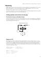
Pipelining ..............................................................................................................................................24
Getting multiple instructions into the pipe..................................................................................25
Functionality, timing, and hardware design.......................................................................25
Mapping to LSE.................................................................................................................25
An alternate mapping to LSE ............................................................................................27
Stalling for control hazards .........................................................................................................29
Functionality, timing, and hardware design.......................................................................29
Mapping to LSE.................................................................................................................30
Performing stalls ......................................................................................................30
A word about state ...................................................................................................31
Generating stalls.......................................................................................................31
Stalling for data hazards ..............................................................................................................34
Functionality, timing, and hardware design.......................................................................34
Mapping to LSE.................................................................................................................34
Stalling for structural hazards .....................................................................................................37
Functionality, timing, and hardware design.......................................................................38
Mapping to LSE.................................................................................................................38
The pipelined timing model ........................................................................................................38
Bypassing..............................................................................................................................................45
Functionality, timing, and hardware design ................................................................................46
Mapping to LSE ..........................................................................................................................46
Performing writeback at completion .................................................................................48
Copying operand values.....................................................................................................48
The bypassing models .................................................................................................................50
iii
3. More complex refinements .........................................................................................................................64
Control speculation ...............................................................................................................................64
Functionality, Timing, and Hardware design ..............................................................................64
Mapping to LSE ..........................................................................................................................64
Removing instructions from the pipe ................................................................................64
Adding a port ...........................................................................................................65
Passing a literal ........................................................................................................66
Stalls and PC update ..........................................................................................................67
Clearing the scoreboard .....................................................................................................67
Dealing with the emulator .................................................................................................68
Recovering from misspeculation when copying operand values .............................68
Recovering from writeback at completion ...............................................................68
The final control speculation models ..........................................................................................70
Out-of-order execution..........................................................................................................................85
Functionality, Timing, and Hardware design ..............................................................................85
Mapping to LSE ..........................................................................................................................85
Renaming...........................................................................................................................86
Wakeup and select .............................................................................................................86
The store buffer..................................................................................................................86
Dealing with misspeculation..............................................................................................87
Ensuring in-order commit..................................................................................................87
Writeback bandwidth change ............................................................................................87
Super-scalar execution ..........................................................................................................................87
Functionality, Timing, and Hardware design ..............................................................................87
Mapping to LSE ..........................................................................................................................87
Multiprocessing.....................................................................................................................................88
Functionality, Timing, and Hardware design ..............................................................................88
Mapping to LSE ..........................................................................................................................88
4. Instruction set emulation ............................................................................................................................89
Concepts................................................................................................................................................89
What is an emulator?...................................................................................................................89
Emulation goals...........................................................................................................................89
Capabilities..................................................................................................................................90
Instructions ..................................................................................................................................91
Operating system emulation........................................................................................................91
Contexts.......................................................................................................................................91
State spaces .................................................................................................................................92
Using the emulation interface ...............................................................................................................93
Declaring the emulator in lss.......................................................................................................93
Datatypes .....................................................................................................................................93
Dealing with multiple emulator instances ...................................................................................94
The most basic tasks .............................................................................................................................95
Creating a dynamic instruction instance .....................................................................................95
Executing an instruction (simple form).......................................................................................96
Finding instruction addresses ......................................................................................................96
Determining when a context is finished ......................................................................................97
Putting it all together ...................................................................................................................97
Other basic tasks ...................................................................................................................................98
Disassembling instructions..........................................................................................................98
Accessing instruction information ..............................................................................................98
iv
Decoding instruction classes .......................................................................................................98
Determining branch targets and direction ...................................................................................99
Comparing the age of instructions ..............................................................................................99
Obtaining state space information...............................................................................................99
Detecting register-carried data dependencies............................................................................100
Obtaining memory access information .....................................................................................101
Detecting memory-carried data dependencies ..........................................................................102
Declaring clocks ........................................................................................................................102
Advanced context handling.................................................................................................................102
Handling context switches.........................................................................................................103
Creating and destroying hardware contexts ..............................................................................103
Accessing state spaces directly .................................................................................................103
More complex tasks ............................................................................................................................104
Executing an instruction (detailed form)...................................................................................104
Manipulating operand values ....................................................................................................105
Source operands...............................................................................................................105
Destination operands .......................................................................................................105
Other considerations ........................................................................................................106
Handling speculation.................................................................................................................106
Avoiding speculation entirely ..........................................................................................108
Issues with imprecise speculation recovery.....................................................................109
5. Device emulation......................................................................................................................................110
Overview.............................................................................................................................................110
Important concepts ....................................................................................................................110
The relationship with ISA emulation ........................................................................................110
Using device emulation within a simulator.........................................................................................111
Configuring a device tree ..........................................................................................................111
Using device emulation wihin an instruction-set emulator.................................................................111
Writing a device emulator...................................................................................................................111
6. Checkpointing...........................................................................................................................................113
Overview.............................................................................................................................................113
Checkpoint file format ........................................................................................................................113
Using the checkpointing interface ......................................................................................................114
Declaring the interface in lss .....................................................................................................114
Datatypes ...................................................................................................................................115
Writing a checkpoint file ...........................................................................................................115
Reading a checkpoint file ..........................................................................................................117
Appending to a checkpoint file..................................................................................................119
Building data trees.....................................................................................................................119
Parsing data trees.......................................................................................................................121
Data buffering details ................................................................................................................123
Managing checkpoint files ..................................................................................................................123
The LSE_chkpt domain .......................................................................................................................124
Using checkpoints from a domain.............................................................................................124
Supporting checkpoints in a module .........................................................................................124
7. Sampling...................................................................................................................................................126
Overview.............................................................................................................................................126
The sampler state machine ........................................................................................................126
Sampler events...........................................................................................................................127
Statistical analysis .....................................................................................................................127
v
Sampling and state-induced bias ...............................................................................................128
Sampling with checkpoints .......................................................................................................128
Using the sampling interface ..............................................................................................................128
Declaring the interface in lss .....................................................................................................129
Datatypes ...................................................................................................................................129
Creating and destroying sampler state machines ......................................................................129
Advancing a sampler state machine ..........................................................................................130
Sampling and the simulation cycle............................................................................................131
Using the sampleController module........................................................................................131
Recording and using statistics ...................................................................................................132
II. Using the LSE tools more effectively.............................................................................................................133
8. Controlling and debugging LSE builds ....................................................................................................134
Debugging scheduling issues ..............................................................................................................134
Controlling simulator code generation................................................................................................135
Code sharing..............................................................................................................................135
Simulator scheduling.................................................................................................................135
Parallel simulation.....................................................................................................................136
Improving simulator performance.............................................................................................138
Other parameters .......................................................................................................................138
9. Static Visualization of LSE Configurations..............................................................................................140
Basic Functionality .............................................................................................................................140
Starting the Visualizer ...............................................................................................................140
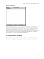
The Visualizer Main Window ..........................................................................................140
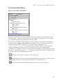
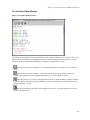
The Visualizer Editor Window ........................................................................................141
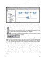
The Visualizer Schematic View Window ........................................................................145
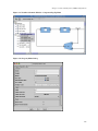
Customizing the Schematic View..............................................................................................148
Customization Primitives.................................................................................................148
Properties ...............................................................................................................148
Customizing the Visual Representation of Canvas Components.....................................149
Customizing the Visual Representation of Instances .............................................149
10. Dynamic Visualization of LSE Configurations ......................................................................................150
Visualizer-side mechanisms................................................................................................................150
Simulator-side mechanisms ................................................................................................................150
III. Extending LSE ...............................................................................................................................................153
11. Extending LSE through domains............................................................................................................154
General concepts.................................................................................................................................154
Writing a single-implementation/shared-code domain class ..............................................................154
Installing the domain class and implementation in the standard LSE installation....................155
Writing a single-implementation/non-shared-code domain class.......................................................155
Adding per-instance identifiers ...........................................................................................................156
Non-managed identifiers ...........................................................................................................156
Managed identifiers ...................................................................................................................157
Merged identifiers ...............................................................................................................................159
Identifier visibility...............................................................................................................................159
Writing a multiple-implementation domain class...............................................................................160
Domain identifiers renaming rules......................................................................................................160
Generating header files .......................................................................................................................161
Identifiers without namespaces or with C linkage ..............................................................................162
Hooks ..................................................................................................................................................162
vi
Structure attributes ..............................................................................................................................164
Chaining domains ...............................................................................................................................165
Generating code at buildtime ..............................................................................................................165
The Python file attributes ....................................................................................................................166
Library specification..................................................................................................................171
Structure of the Python file.......................................................................................................172
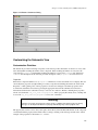
12. The Command-Line Processor ...............................................................................................................174
General concepts.................................................................................................................................174
The standard command line processor................................................................................................174
Interface the command-line processor must provide ..........................................................................175
Interface provided to the command line processor .............................................................................175
Datatypes and variables.............................................................................................................175
APIs for argument parsing ........................................................................................................176
APIs for initialization and finalization ......................................................................................176
APIs for simulator control.........................................................................................................177
13. Writing a new emulator ..........................................................................................................................179
General concepts.................................................................................................................................179
How are emulators interfaced?..................................................................................................179
State and the model of computation ..........................................................................................179
Exception semantics ..................................................................................................................179
Cross-instruction semantics.......................................................................................................180
Preparing an emulator for use with LSE.............................................................................................180
The emulator description file ..............................................................................................................181
The base emulator interface ................................................................................................................184
Datatypes, variables, and functions made available to emulators .............................................184
Functions an emulator must supply...........................................................................................186
Other requirements ....................................................................................................................187
Code sharing ....................................................................................................................187
Context handling..............................................................................................................187
State spaces......................................................................................................................188
Decoding and instruction classes.....................................................................................189
Predecoded information...................................................................................................189
Instruction steps ...............................................................................................................190
Exiting and signal handlers..............................................................................................190
Error reporting .................................................................................................................191
Extra identifiers................................................................................................................191
Extra functions.................................................................................................................191
Header files ......................................................................................................................191
Library names ..................................................................................................................192
Definining emulator-specific header files ........................................................................192
State-space capability definitions........................................................................................................192
The access capability ................................................................................................................192
General capability definitions .............................................................................................................193
The branchinfo capability .........................................................................................................193
The checkpoint capability..........................................................................................................194
The commandline capability .....................................................................................................195
The disassemble capability........................................................................................................195
The operandinfo capability .......................................................................................................196
The operandval capability.........................................................................................................197
The reclaiminstr capability .......................................................................................................198
vii
The speculation capability ........................................................................................................198
The timed capability ..................................................................................................................199
Additional functionality ......................................................................................................................200
Documenting the emulator..................................................................................................................200
14. The Liberty Instruction Specification Language (LIS) ..........................................................................202
Motivation ...........................................................................................................................................202
Using LIS to generate emulator code..................................................................................................202
LIS concepts........................................................................................................................................203
Comments and file management ...............................................................................................203
Literals and identifiers ...............................................................................................................203
Expression Operators ................................................................................................................204
Options and constants................................................................................................................204
Control flow...............................................................................................................................205
Codesections..............................................................................................................................205
Defining emulator attributes......................................................................................................207
Defining types ...........................................................................................................................207
Accessing state spaces...............................................................................................................208
Instruction fields ........................................................................................................................210
Naming operands.......................................................................................................................211
Defining instructions .................................................................................................................212
Opcode attribute...............................................................................................................213
Format attribute................................................................................................................214
Match attribute.................................................................................................................214
Action attribute ................................................................................................................214
Operand attribute .............................................................................................................215
Frequency attribute ..........................................................................................................216
Sharing instruction attributes.....................................................................................................216
Creating groups of instructions .................................................................................................217
Creating multiple levels of granularity......................................................................................218
Capability attribute ..........................................................................................................220
Decoder attribute..............................................................................................................220
Entrypoint attribute ..........................................................................................................221
Step attribute ....................................................................................................................222
Hide and show attributes..................................................................................................222
Styles .........................................................................................................................................223
Assigning an implementation to a buildset......................................................................223
Other stuff ........................................................................................................................223
Completing an emulator described in LIS ..........................................................................................223
LSE emulator functions.............................................................................................................224
Memory statespaces ..................................................................................................................224
Standalone emulator support .....................................................................................................225
Endianness support....................................................................................................................225
Operating system abstraction ....................................................................................................225
Advice about other tasks.....................................................................................................................226
Implementation notes..........................................................................................................................227
viii
IV. Reference materials .......................................................................................................................................228
15. Useful information I haven’t organized yet............................................................................................229
Clocks .................................................................................................................................................230
Organizing a configuration .................................................................................................................230
Common hardware paradigms ............................................................................................................230
A. LSS Reference .........................................................................................................................................231
Basic Syntax........................................................................................................................................231
Basic Data Types .......................................................................................................................231
int ...................................................................................................................................231
float...............................................................................................................................232
boolean ..........................................................................................................................232
char .................................................................................................................................232
string ............................................................................................................................232
literal ..........................................................................................................................232
type .................................................................................................................................233
enumerations....................................................................................................................233
arrays................................................................................................................................233
structures..........................................................................................................................233
functions ..........................................................................................................................234
external Types..............................................................................................................234
pointer Types................................................................................................................235
Comments..................................................................................................................................235
Variable Declaration ..................................................................................................................235
Expressions and Operators ........................................................................................................236
Unary Operator Expressions............................................................................................237
Binary Operators and Expressions...................................................................................237
The Ternary Operator ......................................................................................................240
Assignment Operators .....................................................................................................240
Indexing Expressions.......................................................................................................240
Subfield Expressions........................................................................................................241
Function Invocation Expression ......................................................................................241
Data Initialization Check Expression ..............................................................................241
Expression Substitution via ${} ...............................................................................................242
Statements .................................................................................................................................242
Control Flow ....................................................................................................................243
The if Statement ...................................................................................................243
Loops......................................................................................................................244
The return statement ...........................................................................................244
Including Other Source Files ...........................................................................................245
Declarations .....................................................................................................................245
Variables.................................................................................................................245
Types ......................................................................................................................245
Functions ................................................................................................................246
Conditional Assignment ..................................................................................................246
Built-In Functions .....................................................................................................................246
Machine Construction Constructs.......................................................................................................247
Module Instances.......................................................................................................................247
Creating Module Instances ..............................................................................................247
Parameterizing Module Instances....................................................................................248
ix
Using Parameters ...................................................................................................248
Code-Valued Parameters ........................................................................................249
System Defined Instance Parameters .....................................................................249
Runtime Parameters ...............................................................................................250
Module Instance Connections ...................................................................................................251
Syntax and Semantics ......................................................................................................251
Port Types and Connections ............................................................................................252
Polymorphic Types.................................................................................................252
Type Variables ..............................................................................................252
The Or-Type..................................................................................................253
Constraining Port Types with Connections............................................................253
Constraining Types with the constrain statement..............................................254
Utility Functions ..............................................................................................................254
Augmenting Instance State........................................................................................................254
structadds ....................................................................................................................254
Runtime Variables............................................................................................................255
Modules...............................................................................................................................................255
Module Declaration Syntax.......................................................................................................255
Ports...........................................................................................................................................256
Parameters .................................................................................................................................257
Leaf Modules.............................................................................................................................257
Module Attributes ............................................................................................................258
Port Attributes..................................................................................................................259
Methods and Queries .......................................................................................................259
Events ..............................................................................................................................260
Type Exports ....................................................................................................................260
Hierarchical Modules ................................................................................................................260
Data Collectors....................................................................................................................................261
Packages..............................................................................................................................................262
Using packages..........................................................................................................................263
Usage overview................................................................................................................263
Packages, Subpackages and Naming ...............................................................................263
Building Packages .....................................................................................................................264
Domains ..............................................................................................................................................265
Creating a Domain Class...........................................................................................................265
Domain Types ..................................................................................................................265
Using Domains ..........................................................................................................................266
x
List of Tables
4-1. Standard instruction class names ......................................................................................................................98
4-2. Memory access flags.......................................................................................................................................102
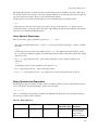
7-1. Sampler parameters ........................................................................................................................................130
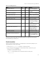
8-1. Code sharing parameters.................................................................................................................................135
8-2. Scheduling parameters....................................................................................................................................135
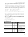
8-3. Parallelization parameters...............................................................................................................................137
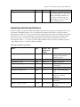
8-4. Performance parameters .................................................................................................................................138
8-5. Other top-level parameters..............................................................................................................................139
13-1. Description file contents ...............................................................................................................................182
13-2. State space types ...........................................................................................................................................188
14-1. Operators.......................................................................................................................................................204
14-2. Codesections .................................................................................................................................................205
14-3. Merging of instruction attributes on inheritance...........................................................................................216
A-1. Binary Operators............................................................................................................................................237
A-2. System-Defined Instance Parameters.............................................................................................................242
A-3. System-Defined Instance Parameters.............................................................................................................249
A-4. Parameter Modifiers.......................................................................................................................................257
A-5. Leaf Module Attributes..................................................................................................................................258
A-6. Port Attributes on Leaf Modules....................................................................................................................259
A-7. Collector Sections ..........................................................................................................................................261
xi
Preface
This book describes how to use LSE to develop simulators and how to use LSE tools more effectively. It includes
information on LSS, debugging, control of simulation parameters, and use of the various APIs available to code
points. For a complete listing of APIs available to configurations, see The Liberty Simulation Environment
Reference Manual
Typographical conventions used in this book
The following typefaces are used in this book:
•
Normal text
•
Emphasized text
• The name of a program variable
• The name of a constant
•
The name of an LSE module
•
The name of a package
•
The name of an domain class
• The name of an attribute in a domain description file
•
The name of an emulator
•
The name of an emulator capability
•
The name of a module parameter
•
The name of a module port
• Literal text
• Text the user replaces
• The name of a file
•
The name of an environment variable
•
The first occurrence of a term
xii
I. Developing Simulation Models in
LSE
We assume that you have read Getting Started with the Liberty Simulation Environment and have learned how to
install and invoke LSE and a little bit about writing configurations and modules. Now you want to use LSE to
develop a useful simulator. This part of the User Manual will help you to develop your own simulators. It
provides our recommendations for how to proceed with the development task. It also provides instructions on how
to use the various LSE domains (extensions).
In the course of these chapters we will develop a model of a simple in-order microarchitecture for a processor
executing the PowerPC instruction set. This simulator will use an LSE emulator which is able to emulate Linux
system calls. We suggest using the crosstool cross-compilation system (available at
http://www.kegel.com/crosstool) to create a gcc cross-compiler to produce PowerPC executables.
Chapter 1. A simple microprocessor model
In this chapter, we develop a simple, non-pipelined, multicycle processor model of a PowerPC microprocesor.
A high-level view of the development process
Designing a complete model can be a daunting task. However, it can be made manageable by following a few
principles and by approaching it in an organized fashion. This section provides a high-level view of these
principles and the process of development.
The first, and most important, principle is simply design hardware, not software. What we mean by this is that you
should always think about how hardware performs the function which you are modeling. LSE is designed to make
it easy to build a model using hardware concepts such as blocks, signals, and state machines. On the other hand,
LSE does not make it quite as easy to use software concepts such as function calls and global variables (though
there are places and times for these, as we will see later in the chapter.) We have found that this hardware focus
not only makes it more natural to use LSE, but also makes it easier to understand and modify the models.
The second principle is develop incrementally. This means that you should not attempt to build the whole model
at once, but should instead refine the model one element at a time, testing the model at each refinement. The next
chapter will illustrate the refinement of processor models.
Tip: Whenever you find yourself stalled in the development of a model, hark back to these two principles:
• Design hardware, not software.
• Develop incrementally
These principles complement each other; models which are more "software-like" often prove to be more
difficult to refine.
The development process can be thought of as having three steps which are repeated as the model is refined.
These three steps are:
1. Determine what functionality and timing the hardware being model should have. Note that this step requires
knowledge of general computer architecture and the specific hardware to be modeled.
2. Think about how you would design hardware with this functionality and timing.
3. Map the functionality and timing to LSE elements, using the hardware design from the previous step as a
guide. This mapping step requires familiarity with the LSE module library and extensions as well as how to
write configurations and/or modules.
Tip: Keep the steps separate. In particular, don’t let the question of mapping "pollute" your understanding of
functionality and timing. Determine those first, then figure out how to make LSE do what you want it to do.
1
Chapter 1. A simple microprocessor model
A simple multicycle processor
We begin the processor development by considering a simple multicycle processor.
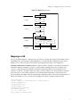
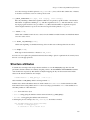
Functionality and timing
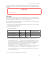
The behavior which the processor must have is given by the following pseudocode:
Figure 1-1. Instruction pseudo-code
forever:
Fetch instruction at current PC
Decode the instruction
Fetch operands
Evaluate results
Calculate new PC
Write back results
Update the PC
In a multicycle processor, this behavior is spread out across multiple clock cycles. For now, we’ll assume that no
pipelining occurs. We will divide the behavior in the following fashion:
forever:
cycle 1:
Fetch instruction at current PC
cycle 2:
Decode the instruction
Fetch operands
cycle 3:
Evaluate results
Calculate new PC
cycle 4:
Write back results
Update the PC
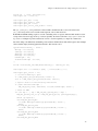
The hardware design
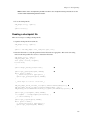
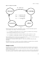
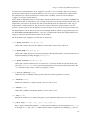
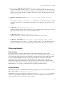
With the behavior divided, we can start to think about the hardware which will be required. A block diagram is
given in Figure 1-2.
Note that the diagram is quite high level; it contains only between-cycle latches and blocks for the major
behaviors. Further refinement of each block into sub-blocks is possible, but not really necessary at this point. Note
also that operand fetching and writeback both happen in the register file.
2
Chapter 1. A simple microprocessor model
Figure 1-2. Multicycle processor
PC
Cycle 1
I mem
Cycle 2
Decode logic
Register file
Cycle 3
ALU / D mem
Calculate new PC
Cycle 4
Mapping to LSE
Now we can map the behavior to LSE constructs. To do this, we consider each element of the hardware in turn,
determining how to describe them as LSE configurations or modules. The final configuration can be seen in
Example 1-1; we will now describe each element of the design and how it maps to the configuration.
Declaring an instruction set emulator. While it would be possible to include all of the instruction behavior in
detail in the simulator configuration, doing so is extremely time-consuming and error-prone. LSE provides
emulators to make this task easier. Emulators are libraries which encapsulate the state and behavior of an
instruction set. The use of emulators makes it possible to share the behavior across many simulators and means
that you don’t have to write detailed simulator code to handle the functional behavior of the instruction set.
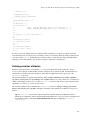
To use an emulator, the emulator must be declared in the configuration. This is done in the following fashion (see
the Section called Declaring the emulator in lss in Chapter 4 for details of what the statements mean):
import LSE_emu;
var emu = LSE_emu::create("emuinst", <<<LSE_PowerPC --include PowerPC64.lis
include PPCLinux.lis
include PPCbuild.lis
include PowerPC_compat.lis
show maximal queue;
>>>, "") : domain ref;
add_to_domain_searchpath(emu);
3
Chapter 1. A simple microprocessor model
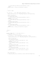
The PC. The PC is easily modeled using the delay module from the core library. The delay module works much
like a flop; during a clock cycle it outputs a stored value. At the end of the clock cycle the stored value is thrown
away and the new value arriving on the input port is stored; however, both these only occur if the output port’s
acknowledge signal is asserted (has the value LSE_signal_ack). The qualification with acknowledge gives basic
flow control behavior.
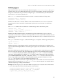
The PC needs to have an initial value to start simulation. Initial values can be set for delay module instances by
filling in the initial_state user point. The initial value for the PC can be read from the emulator using the
LSE_emu_get_start_addr function. The following code will do the trick:
1
2
3
4
5
6
7
8
9
10
11
using corelib;
Use core library modules
instance PC : corelib::delay;
Instantiate the PC
PC.initial_state = <<<
*init_id = LSE_dynid_create();
LSE_emu_init_instr(*init_id, 1,
LSE_emu_get_start_addr(1));
Create new dynid
And initialize it
with starting PC
return TRUE; // we set an initial state
>>>;
Tip: The text which you assign to a user point becomes the body of a function with a specific signature. Your
code can use the function parameters even though they are not defined in the LIS file. This can make it hard
to read user point code until you become accustomed to the parameter naming conventions in the LSE
libraries. Consult The Liberty Simulation Environment Reference Manual for the signatures of each user point
of each module in the libraries.
The code used for the initial_state user point must create a new dynamic identifier (dynid for short). This is
required because every time data is sent in the LSE system, a dynid must be sent with it. Thus the delay module
stores a dynid along with the data. A dynid is implemented as a pointer to a heap-allocated, reference-counted
data structure. They are used to "tie" related data transmissions together and to store information which is to be
shared among many different portions of the model without having to copy the data multiple times. For example,
emulators store all the transient information about an instruction inside of the dynid. Thus lines 7-8 explicitly
initialize the dynid to represent the instruction which will be fetched at the new PC.
The function arguments equal to 1 on lines 7 and 8 are emulator context numbers. Because emulators may
emulate operating system behavior, the LSE emulation subsystem provides support for "virtualization" of the
hardware resources and context switching. This is done by declaring hardware thread contexts and software
thread contexts and mapping them together. By default, one hardware context is created whenever there is an
emulator. The ’1’ is the identifier of this default hardware context. More information about contexts is found in
Chapter 4. For now, we need only deal with them when setting the initial PC.
Another question which must be resolved is what data (and data type) should be stored for the PC. The natural
choice is the emulated PC itself, of type LSE_emu_iaddr_t, which is the data type the emulator supplies for
instruction addresses. However, the address of the instruction is already stored within the dynid, so storing it again
is redundant. You may find it more natural to store it anyway, but for this example we will not store it again. Thus
no data beyond the dynid is stored in the PC instance and the datatypes of its connections will be none.
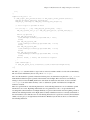
Inter-cycle latches. Latches can also be modeled quite simply by delay modules. The default flow-control
behavior works well. We will instantiate them as indicated in Figure 1-2, with two instances for the bottom delay
element. This is for convenience, as the two signal paths indicated for the bottom may have different datatypes
4
Chapter 1. A simple microprocessor model
and the delay module, while it can have multiple parallel signal paths, must have the same datatype on all of
them. The code to instantiate these elements is:
instance
instance
instance
instance
IF_ID_latch
ID_EX_latch
EX_WB_latch
newPC_latch
:
:
:
:
corelib::delay;
corelib::delay;
corelib::delay;
corelib::delay;
Instruction memory (I mem). The current hardware design assumes a constant 1 cycle access time to instruction
memory. Thus there is no need to model a memory in detail. All that is needed is to ask the emulator to perform
the instruction fetch from its memory. This is done by calling the LSE_emu_do_instrstep function.
Emulators break up instruction behavior into a series of steps, much like those listed in Figure 1-1. The exact
sequence of steps depends upon the emulator, and is included in the emulator’s documentation found in The
Liberty Simulation Environment Reference Manual for emulators supplied with LSE. In the case of the PowerPC
emulator, the steps are: ifetch, decode, opfetch, evaluate, ldmemory, format, writeback. The identifier for the step
is formed by prepending LSE_emu_instrstep_name_ to the step name.
Of course, we also need some way to make this emulator call in the LSE model. There are several ways of doing
this, but the simplest to think about is to use a converter module. The converter is really a "monadic function"
module; it takes a single input signal and computes a single output signal from it. The types of the input and
output signal need not be the same, hence the name "converter", as in "type conversion". The user of the converter
module must supply the conversion function via the convert_func user point.
We can view our use of the converter module as a means to compute the "fetch instruction" function. The
converter module is preferred over alternate means of performing this behavior because it is a standard module
and because it only calls the user point once per cycle per port instance, thus allowing us to write user points
which might be expensive (as calling the emulator often is) more efficiently. The code we use is:
instance Imem : corelib::converter;
PC.out
-> [none] Imem.in;
Imem.out -> [none] IF_ID_latch.in;
Imem.convert_func = <<<
LSE_emu_do_instrstep(id, LSE_emu_instrstep_name_ifetch);
return data;
Return the (dummy) input data
>>>;
Note that both connections to the Imem instance explicitly state the datatype. The connection from PC needs an
explicit datatype because we have not yet indicated PC’s datatype. This explicit statement is also sufficient to
imply the datatype of the input port of PC. On the other hand, because converter modules can change types, type
inference cannot infer that the output type of Imem is the same as its input type. Thus the output connection must
explicitly state the datatype.
Decode logic. The decode logic can also be performed completely by the emulator. Thus the decode logic can be
modeled as another converter module which calls the emulator:
instance Decode : corelib::converter;
IF_ID_latch.out -> Decode.in;
Decode.convert_func = <<<
LSE_emu_do_instrstep(id, LSE_emu_instrstep_name_decode);
return data;
Return the (dummy) input data
5
Chapter 1. A simple microprocessor model
>>>;
Register file. The register file has two functions to perform: reading of register operands and writeback of register
operands. Reading should occur during the clock cycle. Writeback should occur at the end of the clock cycle.
Reading of operands can be accomplished by asking the emulator to perform the opfetch step, and writing by
performing the writeback step.
While there are modules in the library which can perform behavior during the clock cycle for one set of ports and
at the end of the clock cycle for a different set of ports (e.g. state_combiner), such modules are fairly complex to
use. A simpler solution in this case is to simply use two module instances to handle the register file. This is
particularly appropriate as the state which is being shared between the instances (the register file values) is inside
the emulator instead of the simulator. The first module is simply a converter used to fetch the register operands.
The second module is a sink module; this module simply takes an input at the end of the clock cycle and produces
no output.
There is one complication. The writeback step actually writes back both register and memory operands in this
emulator. However, the register file is not the "right place" to write back memory operands, and, in the simple
machine we are envisioning, write back of memory operands should happen one cycle earlier. Fortunately, this
does not present a major problem, as the register file writeback can ask the emulator to only write back operands
which have not yet been written back; the LSE_emu_writeback_remaining_operands does this. The
following code is what we want:
instance regRead : corelib::converter;
instance regWrite : corelib::sink;
Decode.out -> [none] regRead.in;
regRead.out -> [none] ID_EX_latch.in;
EX_WB_latch.out -> regWrite.in;
regRead.convert_func = <<<
LSE_emu_do_instrstep(id, LSE_emu_instrstep_name_opfetch);
return data;
Return the (dummy) input data
>>>;
regWrite.sink_func = <<<
if (LSE_signal_data_present(status) && LSE_signal_enable_present(status)) {
LSE_emu_writeback_remaining_operands(id);
LSE_emu_do_instrstep(id, LSE_emu_instrstep_name_exception);
}
>>>;
The sink_func user point defines behavior to take place at the end of the clock cycle for each input port instance
of the in port of a sink instance. The user point is called whether there is data or not; thus the emulator call has
been guarded with a check to see if there actually is data. It is also gated with a check whether the data is enabled;
this check allows flow control logic to prevent the writeback from occurring.
Note: The LSE mapping has been influenced here by the way in which the emulator is written, particularly the
granularity of its steps. If the emulator had separated writeback of register operands from writeback of
memory operands into separate steps, the register file logic would have been simpler. If the emulator had not
had the operandval capability, individual operand manipulation would not have been possible. Bear this in
mind if you happen to develop an emulator.
6
Chapter 1. A simple microprocessor model
ALU and data memory (D mem). The behavior of the ALU as well as reads of data memory can be performed
via emulator steps. Writes to data memory for store instructions require writeback of the memory operand; we can
write back just this one operand by calling LSE_emu_writeback_operand with the name of the memory
operand (which is mem in the PowerPC emulator.) Because all of the behavior can be done with emulator calls, we
again use a converter module:
Referring back to Figure 1-2, we can see that there is a "tee" — or a place with fanout — in the hardware diagram
during the 3rd cycle. Fanout is introduced in LSE primarily through tee module instances. The tee fans out the
data and enable signals in the forward (in-to-out) direction and combines the acknowledge signals in the
backward direction. The default is to logically AND the acknowledge signals together, which means
"acknowledge only if all destinations acknowledge". The default behavior can be changed with parameters. For
the moment, we will insert the tee, but only make a single output connection.
instance EXtee : corelib::tee;
instance ALUmem : corelib::converter;
ID_EX_latch.out -> EXtee.in;
EXtee.out
-> ALUmem.in;
ALUmem.out
-> [none] EX_WB_latch.in;
ALUmem.convert_func = <<<
LSE_emu_do_instrstep(id, LSE_emu_instrstep_name_evaluate);
LSE_emu_do_instrstep(id, LSE_emu_instrstep_name_ldmemory);
if (LSE_emu_dynid_is(id, store))
LSE_emu_writeback_operand(id, LSE_emu_operand_name_destMem);
return data;
>>>;
New PC calculation. In the PowerPC emulator, the new PC calculation takes place when the emulate step is
performed by the ALU and data memory. Thus there is no need for a separate new PC calculation module.
However, there is a need to create a new dynid within the feedback path from the last latch to the PC. This can be
done once again by using a converter module. The convert_func user point allows us to change the dynid,
substituting a new one, as well as the data.
At this point, we can make a second connection to the tee in the 3rd cycle and attach the new dynid creator
instance:
instance newDynid : corelib::converter;
EXtee.out -> newPC_latch.in;
newPC_latch.out -> newDynid.in;
newDynid.out -> [none] PC.in;
newDynid.convert_func = <<<
*newidp = LSE_dynid_create();
LSE_dynid_cancel(*newidp);
See below
if (LSE_emu_get_context_mapping(1) == LSE_emu_dynid_get(id, swcontexttok))
LSE_emu_init_instr(*newidp, 1, LSE_emu_dynid_get(id, next_pc));
else if (LSE_emu_get_context_mapping(1))
LSE_emu_init_instr(*newidp, 1, LSE_emu_get_start_addr(1));
else LSE_emu_init_instr(*newidp, 1, LSE_emu_dynid_get(id, addr));
return data;
>>>;
7
Chapter 1. A simple microprocessor model
The new dynid creation is very much like the creation of the initial dynid in the PC instance. The difference is how
we find the address of the new instruction. If the software context mapped to the default hardware context has not
changed as a result of the instruction’s execution (which could happen if the instruction was an emulated system
call which led to a context switch), then the address is found by looking at the calculated next_pc field of the
instruction we just evaluated. On the other hand, if the software context has changed, the new address is obtained
directly from the context, just as was done when the initial dynid was created. Note that we also check whether
there is any software context mapped at all, as the LSE_emu_get_start_addr call cannot be made (indeed, it
may dump core) when there is no context mapped. This would occur when the emulated program has exited and
the emulator will terminate simulation in the next cycle.
Calling LSE_dynid_create results in a single reference to the dynid. Because this instance does not hold onto
the reference beyond the end of the cycle, it must notify LSE by calling LSE_dynid_cancel by the end of the
cycle. Canceling the reference immediately is legal because dynids without references are only garbage-collected
between clock cycles.
Note: You may have noticed that there is no "data flow" between the instance which produces the new PC
information (ALUmem) and the instance which consumes the new PC information (newDynid). This is not an
error; it works because the information is stored in the dynid, the same dynid has been sent to both instances,
and the consumer uses it in the cycle after it is produced. If the information were to be consumed in the same
cycle, we would need to ensure that the consumer executes after the producer, either through data flow
between the instances or through a control function which waits for the producer to execute before allowing
the consumer to see the new data.
Observations, odds and ends. You may be wondering how the simulator knows when the simulated program has
finished. This is taken care of inside of the emulator. By default, when there are emulators present, LSE
simulators stop simulation when all of the emulators report that they no longer have valid programs mapped.
Another question you may have is how this design, which looks like a pipelined machine, keeps from pipelining
instruction execution. The key here is that there is only one dynid at a time in the model. The initial dynid in the
PC instance flows through the physical pipeline of modules, but the PC does not inject a new dynid after the initial
one leaves. Only at the bottom of the pipeline as an instruction completes execution does a new dynid get created
for the next instruction and sent to PC.
The resulting configuration
Example 1-1. The complete multicycle processor model
multicycle.lss
import LSE_emu;
var emu = LSE_emu::create("emuinst", <<<LSE_PowerPC -include PowerPC64.lis
include PPCLinux.lis
include PPCbuild.lis
include PowerPC_compat.lis
show maximal queue;
>>>, "") : domain ref;
add_to_domain_searchpath(emu);
using corelib;
8
Chapter 1. A simple microprocessor model
instance
instance
instance
instance
instance
instance
instance
instance
instance
instance
instance
instance
PC
Imem
IF_ID_latch
Decode
regRead
regWrite
ID_EX_latch
EXtee
ALUmem
EX_WB_latch
newPC_latch
newDynid
:
:
:
:
:
:
:
:
:
:
:
:
corelib::delay;
corelib::converter;
corelib::delay;
corelib::converter;
corelib::converter;
corelib::sink;
corelib::delay;
corelib::tee;
corelib::converter;
corelib::delay;
corelib::delay;
corelib::converter;
PC.initial_state = <<<
*init_id = LSE_dynid_create();
LSE_emu_init_instr(*init_id, 1, LSE_emu_get_start_addr(1));
return TRUE; // we set an initial state
>>>;
PC.out
-> [none] Imem.in;
Imem.convert_func = <<<
LSE_emu_do_instrstep(id, LSE_emu_instrstep_name_ifetch);
return data;
>>>;
Imem.out
-> [none] IF_ID_latch.in;
IF_ID_latch.out -> Decode.in;
Decode.convert_func = <<<
LSE_emu_do_instrstep(id, LSE_emu_instrstep_name_decode);
return data;
>>>;
Decode.out
-> [none] regRead.in;
regRead.convert_func = <<<
LSE_emu_do_instrstep(id, LSE_emu_instrstep_name_opfetch);
return data;
>>>;
regWrite.sink_func = <<<
if (LSE_signal_data_present(status) && LSE_signal_enable_present(status)) {
LSE_emu_writeback_remaining_operands(id);
LSE_emu_do_instrstep(id, LSE_emu_instrstep_name_exception);
}
>>>;
regRead.out
ID_EX_latch.out
EXtee.out
EXtee.out
->
->
->
->
[none] ID_EX_latch.in;
EXtee.in;
ALUmem.in;
newPC_latch.in;
ALUmem.convert_func = <<<
9
Chapter 1. A simple microprocessor model
LSE_emu_do_instrstep(id, LSE_emu_instrstep_name_evaluate);
LSE_emu_do_instrstep(id, LSE_emu_instrstep_name_ldmemory);
if (LSE_emu_dynid_is(id, store))
LSE_emu_writeback_operand(id, LSE_emu_operand_name_destMem);
return data;
>>>;
ALUmem.out
-> [none] EX_WB_latch.in;
EX_WB_latch.out -> regWrite.in;
newPC_latch.out -> newDynid.in;
newDynid.out
-> [none] PC.in;
newDynid.convert_func = <<<
*newidp = LSE_dynid_create();
LSE_dynid_cancel(*newidp);
if (LSE_emu_get_context_mapping(1) == LSE_emu_dynid_get(id, swcontexttok))
LSE_emu_init_instr(*newidp, 1, LSE_emu_dynid_get(id, next_pc));
else if (LSE_emu_get_context_mapping(1))
LSE_emu_init_instr(*newidp, 1, LSE_emu_get_start_addr(1));
else LSE_emu_init_instr(*newidp, 1, LSE_emu_dynid_get(id, addr));
return data;
>>>;
A much simpler mapping to LSE
The mapping to LSE presented in the previous subsection is actually much more complex than it needs to be,
though it is desirable because of its flexibility and clarity. This subsection presents a far simpler, yet less flexible,
model which runs about three times faster. Our purpose in presenting this model is to emphasize that the
granularity of modeling is up to you and should be chosen to meet your goals.
The simpler model rests upon the observation that the timing is fixed at 4 cycles for every instruction and it really
does not matter in which of the cycles the instruction behavior is modeled. Thus we can replace all of the
inter-cycle latches with a simple delay of 3 cycles and can perform all of the emulation when we need to calculate
the new PC.
To create a 3 cycle delay, we use the pipe module. This module acts in its simplest configuration like a pipeline of
delay instances. The amount of delay is set by assigning 3 to the depth parameter of the pipe instance.
We perform all of the emulation and new PC generation in a converter instance. The calls to the emulator use
functions LSE_emu_dofront and LSE_emu_doback; . these functions perform multiple steps and together
completely emulate an instruction. The final code for this configuration is:
Example 1-2. The much simpler multicycle processor model
multicycle2.lss
import LSE_emu;
var emu = LSE_emu::create("emuinst", <<<LSE_PowerPC -include PowerPC64.lis
include PPCLinux.lis
include PPCbuild.lis
10
Chapter 1. A simple microprocessor model
include PowerPC_compat.lis
show maximal queue;
>>>, "") : domain ref;
add_to_domain_searchpath(emu);
using corelib;
instance PC
instance pipeline
instance newPC
: corelib::delay;
: corelib::pipe;
: corelib::converter;
PC.initial_state = <<<
*init_id = LSE_dynid_create();
LSE_emu_init_instr(*init_id, 1, LSE_emu_get_start_addr(1));
return TRUE; // we set an initial state
>>>;
PC.out -> [none] pipeline.in;
pipeline.depth = 3;
pipeline.out -> newPC.in;
newPC.convert_func = <<<
LSE_emu_dofront(id);
LSE_emu_doback(id);
*newidp = LSE_dynid_create();
LSE_dynid_cancel(*newidp);
if (LSE_emu_get_context_mapping(1) == LSE_emu_dynid_get(id, swcontexttok))
LSE_emu_init_instr(*newidp, 1, LSE_emu_dynid_get(id, next_pc));
else if (LSE_emu_get_context_mapping(1))
LSE_emu_init_instr(*newidp, 1, LSE_emu_get_start_addr(1));
else LSE_emu_init_instr(*newidp, 1, LSE_emu_dynid_get(id, addr));
return data;
>>>;
newPC.out -> PC.in;
Reporting simulator behavior and results
By default, LSE simulators print the number of cycles which simulation took, but no other results. Any other
output must be specified through the configuration, typically by writing data collectors. Data collectors are
snippets of code that are run when events occur. We will demonstrate several in the following subsections.
11
Chapter 1. A simple microprocessor model
Counting instructions
Our first example of a data collector counts completed instructions. In this particular model, all completed
instructions eventually reach the regWrite sink. So we attach a collector on the SUNK_DATA event, which is
triggered at the end of a timestep when data is sunk. (Note that the sink_func userpoint has already been used
by the model, so we can’t reuse it. In general, you should not use a user point to report behavior because doing so
can disrupt model behavior.) However, every module has an end_of_timestep event. This event is triggered on
every cycle. Thus, we can fill in this event with a check to see whether data has arrived in the cycle; if it has, then
we increment the instruction count:
{
var icount = new runtime_var("icount", uint64) : runtime_var ref;
collector SUNK_DATA on "regWrite" {
init
= <<< ${icount} = 0; >>>;
record = <<< ${icount}++; >>>;
report = <<<
std::cerr << "Total instructions executed: " << ${icount} << std::endl;
>>>;
};
}
The variable which is used to record the instruction count is an LSS runtime variable. LSS runtime variables
produce a variable in the generated simulator. This variable is guaranteed to have a unique name. The odd "${}"
notation is used inside of the triple-angle-brackets to indicate that the result of an LSS should be inserted into the
string; for runtime variables, the inserted result is the generated variable’s name.
Tip: Note that both the runtime variable definition and the collector are placed inside of curly braces. While
not totally necessary, doing this restricts the icount variable’s scope to only the block inside the curly braces.
Doing so prevents name clashes with other LSS variables which may happen to be named icount when the
configuration is parsed.
Tracing completed instructions
We can trace completed instructions by adding another data collector at the same location where we counted the
completed instructions. This data collector prints the time, the id number of the instruction’s dynid, asks the
emulator to disassemble the instruction, and calls an emulator-specific "extra" function which prints out the
operand values of the instruction:
collector SUNK_DATA on "regWrite" {
record = <<<
std::cerr << LSE_time_now << ": id:" << LSE_dynid_get(id, idno) << " ";
LSE_emu_disassemble(id, stderr);
LSE_emu_call_extra_func(PPC_print_instr_oper_vals, stderr, "",
& LSE_dynid_get(id, attr:emuinst:instr_info));
>>>;
};
The odd construction inside of LSE_dynid_get is used to get a pointer to the instruction information in the
dynid; this is needed because the extra function for operands does not understand dynids.
12
Chapter 1. A simple microprocessor model
What if we don’t want to disassemble every instruction every time we run the simulator, but just sometimes?
While we can certainly build two different simulators, one with and one without the collector, matters quickly get
out of hand if there is more than one behavior to turn off or on. A better way of handling this is through runtime
parameters. A run-time parameter is a parameter which can be set from the command line of the simulator. To
create a runtime parameter, declare a runtimeable parameter and assign a runtime_parm object to it. Then use
the parameter via the ${} notation. For example, to control instruction tracing from the command line, use the
following:
runtimeable parameter dotrace = new runtime_parm(boolean, false, "trace",
"Turn on instruction tracing") : boolean;
collector SUNK_DATA on "regWrite" {
record = <<<
if (${dotrace}) {
std::cerr << LSE_time_now << ": id:" << LSE_dynid_get(id, idno) << " ";
LSE_emu_disassemble(id, stderr);
LSE_emu_call_extra_func(PPC_print_instr_oper_vals, stderr, "",
& LSE_dynid_get(id, attr:emuinst:instr_info));
}
>>>;
};
The first argument of the runtime_parm constructor gives the type of the parameter, the second argument is the
default value, the third argument is the command-line option’s text, and the final argument is a description that
will be printed when --help is given on the command-line. The user can turn on tracing with the command-line
option --sim:trace=true.
Note: Run-time parameters cannot control the structure of the simulator (e.g. the number of connections
made). In general, if you need to know it at build-time, a run-time parameter can’t set it.
Tracing instructions moving through stages
This series of collectors tracks instructions moving through the simulated machine. It reports the cycle at which
each instruction arrives in each inter-cycle latch. The information reported for each instruction is its address and
its dynid id number (each dynid has a unique id number.)
runtimeable parameter dostagetrace
= new runtime_parm(boolean, false, "stagetrace",
"Turn on stage tracing") : boolean;
collector STORED_DATA on "IF_ID_latch" {
record = <<<
if (${dostagetrace})
std::cerr << LSE_time_now << ": IF "
<< "id:" << LSE_dynid_get(id,idno) << " addr:"
<< std::hex << LSE_emu_dynid_get(id, addr) << std::dec
<< std::endl;
>>>;
};
collector STORED_DATA on "ID_EX_latch" {
13
Chapter 1. A simple microprocessor model
record = <<<
if (${dostagetrace})
std::cerr << LSE_time_now << ": ID "
<< "id:" << LSE_dynid_get(id,idno) << " addr:"
<< std::hex << LSE_emu_dynid_get(id, addr) << std::dec
<< std::endl;
>>>;
};
collector STORED_DATA on "EX_WB_latch" {
record = <<<
if (${dostagetrace})
std::cerr << LSE_time_now << ": EX "
<< "id:" << LSE_dynid_get(id,idno) << " addr:"
<< std::hex << LSE_emu_dynid_get(id, addr) << std::dec
<< std::endl;
>>>;
};
collector SUNK_DATA on "regWrite" {
record = <<<
if (${dostagetrace})
std::cerr << LSE_time_now << ": WB "
<< "id:" << LSE_dynid_get(id,idno) << " addr:"
<< std::hex << LSE_emu_dynid_get(id, addr) << std::dec
<< std::endl;
>>>;
};
All the data collectors
Example 1-3. Data collectors for the simple model
multicycleEvents.lss
{
var icount = new runtime_var("icount", uint64) : runtime_var ref;
collector SUNK_DATA on "regWrite" {
init
= <<< ${icount} = 0; >>>;
record = <<< ${icount}++; >>>;
report = <<<
std::cout << "Total instructions executed: " << ${icount} << std::endl;
>>>;
};
}
runtimeable parameter dotrace = new runtime_parm(boolean, false, "trace",
"Turn on instruction tracing") : boolean;
collector SUNK_DATA on "regWrite" {
record = <<<
if (${dotrace}) {
14
Chapter 1. A simple microprocessor model
std::cerr << LSE_time_now << ": id:" << LSE_dynid_get(id, idno) << " ";
LSE_emu_disassemble(id, stderr);
LSE_emu_call_extra_func(PPC_print_instr_oper_vals, stderr, "",
& LSE_dynid_get(id, attr:emuinst:instr_info));
}
>>>;
};
runtimeable parameter dostagetrace
= new runtime_parm(boolean, false, "stagetrace",
"Turn on stage tracing") : boolean;
collector STORED_DATA on "IF_ID_latch" {
record = <<<
if (${dostagetrace})
std::cerr << LSE_time_now << ": IF "
<< "id:" << LSE_dynid_get(id,idno) << " addr:"
<< std::hex << LSE_emu_dynid_get(id, addr) << std::dec
<< std::endl;
>>>;
};
collector STORED_DATA on "ID_EX_latch" {
record = <<<
if (${dostagetrace})
std::cerr << LSE_time_now << ": ID "
<< "id:" << LSE_dynid_get(id,idno) << " addr:"
<< std::hex << LSE_emu_dynid_get(id, addr) << std::dec
<< std::endl;
>>>;
};
collector STORED_DATA on "EX_WB_latch" {
record = <<<
if (${dostagetrace})
std::cerr << LSE_time_now << ": EX "
<< "id:" << LSE_dynid_get(id,idno) << " addr:"
<< std::hex << LSE_emu_dynid_get(id, addr) << std::dec
<< std::endl;
>>>;
};
collector SUNK_DATA on "regWrite" {
record = <<<
if (${dostagetrace})
std::cerr << LSE_time_now << ": WB "
<< "id:" << LSE_dynid_get(id,idno) << " addr:"
<< std::hex << LSE_emu_dynid_get(id, addr) << std::dec
<< std::endl;
>>>;
};
15
Chapter 2. Refinements to the simple
microprocessor model
This chapter demonstrates a number of refinements to the simple processor model.
Non-uniform instruction timing
The multicycle model took four cycles for every instruction. Our next model will provide non-uniform timing.
Functionality, Timing, and Hardware design
The functionality of the processor doesn’t really change; instructions still must be executed in the same fashion.
The only difference is in the timing of the evaluate portion of the instruction. For our example, we will have loads
and stores take two cycles to evaluate, floating point operations take four cycles, and integer operations take one
cycle (as before).
The hardware design would change within the ALU/Dmem block of Figure 1-2. Instead of a single block, we
would have:
Figure 2-1. Inside the ALU/Dmem block
Route instruction
FP
Integer
Memory
The blocks where the actual work of each instruction is done have been left out for clarity. Note that the new PC
calculation or results must also be delayed by the same amount in the hardware; what is likely is that the
calculation would take place at the same time as before, but the results would be moved through the inter-cycle
latches to stay in sync with the instruction evaluation.
16
Chapter 2. Refinements to the simple microprocessor model
Mapping to LSE
This model enhancement starts to show how LSE’s structural nature can make mapping easy. We will replace the
converter instance (named ALUmem) with an instance of a new hierarchical module (i.e. a module which includes
other module instances) which will hold the new ALU/Dmem behavior. We’ll call this module the exPipes
module.
Tip: We could just add new elements to the top-level configuration rather than create a new module. The
amount of hierarchy to create in a design is a design decision you must make. The addition of hierarchy may
make a design easier to understand and visualize. Adding hierarchy can both ease reuse (when you want to
reuse the module without changes) or complicate it (when you need access to internal elements of the
module.)
We could also define the new module as a new leaf module. This is rather more complex, particularly for
behaviors which are to take place across multiple cycles. We will defer discussion of leaf modules until later.
Defining a hierarchical module (exPipes)
To define a hierarchical module, simply use the following syntax in LSS:
module exPipes {
using corelib;
So we can use library modules
all the stuff inside the module
};
It is customary, but not required, to place new hierarchical modules within separate lss files with file names
which match the module name. We will do so in this example; thus the file name will be exPipes.lss.
Since we are trying to write this module as a replacement for the converter module we used before, it should have
an input port named in and an output port named out. Their types could be none, but to make the module more
flexible, we will not constrain them in the module definition. Ports are defined with the inport and outport
statements. Unconstrained types are specified using a type variable; type variables are indicated by prefixing the
variable name with a single quote (’) character. The code to define the ports we want is:
inport in : ’a;
outport out : ’b;
Structure of the module. The overall structure of the module is very similar to Figure 2-1. The modeling of each
portion is described below.
The floating-point unit. The floating point unit must take 4 cycles to process an instruction and must call the
emulator to evaluate the instruction (remember, this is 3 steps in the PowerPC emulator). This can be done easily
with a pipe followed by a converter:
instance FP
instance FPExec
: corelib::pipe;
: corelib::converter;
FP.depth = 3;
FP.out -> FPExec.in;
FPExec.convert_func = <<<
LSE_emu_do_instrstep(id, LSE_emu_instrstep_name_evaluate);
LSE_emu_do_instrstep(id, LSE_emu_instrstep_name_ldmemory);
>>>;
17
Chapter 2. Refinements to the simple microprocessor model
The memory unit. The memory unit must take 2 cycles to process an instruction and must call the emulator to
evaluate the instruction. This can be done most simply with a delay followed by a converter, but to make things
interesting, we will separate the calculation of the effective address (in the evaluate step) from the actual memory
access (the ldmemory, format, and writeback of memory):
instance effAddr
: corelib::converter;
instance EX_MEM_latch : corelib::delay;
instance MemExec
: corelib::converter;
effAddr.out -> [none] EX_MEM_latch.in;
EX_MEM_latch.out -> MemExec.in;
effAddr.convert_func = <<<
LSE_emu_do_instrstep(id, LSE_emu_instrstep_name_evaluate);
>>>;
MemExec.convert_func = <<<
LSE_emu_do_instrstep(id, LSE_emu_instrstep_name_ldmemory);
if (LSE_emu_dynid_is(id, store))
LSE_emu_writeback_operand(id, LSE_emu_operand_name_destMem);
>>>;
The integer unit. The floating point unit must take 1 cycle to process and instruction; like its brethren, it must call
the emulator to evaluate the instruction. This requires only a converter:
instance IntExec
: corelib::converter;
IntExec.convert_func = <<<
LSE_emu_do_instrstep(id, LSE_emu_instrstep_name_evaluate);
LSE_emu_do_instrstep(id, LSE_emu_instrstep_name_ldmemory);
>>>;
Routing to the units. The routing logic at the top of the exPipes module must select between the three different
units based upon the instruction type. There are several modules in the core library which can be used for routing.
The module which best matches this situation (selection of one possible output based upon the input data or
dynid) is the demux module. As its name suggests, this module is a demultiplexer. To use it, we must connect
each of the possible units to its output and then fill in the choose_logic userpoint:
instance routeEx
: corelib::demux;
in -> routeEx.in;
routeEx.out -> FP.in;
routeEx.out -> effAddr.in;
routeEx.out -> IntExec.in;
routeEx.choose_logic = <<<
if (LSE_emu_dynid_is(id, load) || LSE_emu_dynid_is(id, store))
return 1;
else if (LSE_emu_dynid_get(id, queue) == LSE_emu::PPC_FPU_Queue)
return 0;
else return 2;
>>>;
The demux is organized as a parallel set of demux logic. Each input port instance can be routed to one of N output
port instances. The choose_logic function must return a number between 0 and (N-1). In our example, the
18
Chapter 2. Refinements to the simple microprocessor model
units are connected in the order: FP, memory, integer. Thus choose_logic function should return 0 for FP
instructions, 1 for memory instructions, and 2 for other instructions. This is done by looking at the emulator’s
standard instruction classifications (LSE_emu_dynid_is) and fields defined by the emulator and stored in the
dynid.
Tip: Always read the emulator documentation carefully to learn what decoding information is made available
to the simulator. If the emulator does not provide the information, you will need to write some amount of
decoding logic yourself.
Selecting results from the units. The last element of the exPipes module multiplexes or selects among the results
of each unit. There are several different modules in the core library which can be used to do this. The most
appropriate module is the aligner module. The aligner module selects the "first" input port instance which has
data and passes its data to the output port. It can be thought of as an arbiter with a fixed priority function based
upon the port instance number.
Because there is no more than one instruction at a time in flight, the order in which we connect the units is
irrelevant. However, to make the module useful in more situations, we connect the units in inverse order of their
latency; this ensures that the "oldest" instruction is always chosen.
instance EXmux
: corelib::aligner;
FPExec.out -> EXmux.in;
MemExec.out -> EXmux.in;
IntExec.out -> EXmux.in;
EXmux.out -> out;
Using the exPipes module
There are four steps necessary to use the new module:
1. Include the new module definition by adding the following line near the top of the main configuration file:
include "exPipes.lss";
2. Change the instance command for ALUmem to refer to the new module:
instance ALUmem : exPipes;
3. Remove the convert_func assignment from ALUmem.
4. The new PC calculation’s timing must be synchronized with the rest of the instruction execution. The
simplest way to do this is to move the EXtee instance later in the execute logic so that it comes after ALUmem.
Doing so is extremely robust; no change in ALUmem will disturb the synchronization.
ID_EX_latch.out
ALUmem.out
EXtee.out
EXtee.out
->
->
->
->
ALUmem.in;
[none] EXtee.in;
EX_WB_latch.in;
newPC_latch.in;
Another way to do this is to use the pipe module’s variable latency abilities; this approach is slower, odd
looking, and not as robust (in that it must be changed whenever ALUmem changes), but variable latencies are
sometimes useful:
instance newPC_latch : corelib::pipe;
19
Chapter 2. Refinements to the simple microprocessor model
newPC_latch.depth = 4;
newPC_latch.delay_for_send = <<<
if (LSE_emu_dynid_is(id, load) || LSE_emu_dynid_is(id, store))
return 2;
else if (LSE_emu_dynid_get(id, queue) == LSE_emu::PPC_FPU_Queue)
return 4;
else return 1;
>>>;
Note: The attentive reader may realize that we could have built the exPipes module out of a single pipe
followed by a combiner in much the same fashion. However, such an approach wouldn’t have allowed us to
demonstrate hierarchy quite as successfully, nor would it have allowed us to separate the timing of effective
address generation from memory accesses.
The complete non-uniform timing model
Example 2-1. The complete non-uniform timing processor model
exPipes.lss
module exPipes {
using corelib;
inport in : ’a;
outport out : ’b;
instance
instance
instance
instance
instance
instance
instance
instance
routeEx
FP
FPExec
effAddr
EX_MEM_latch
MemExec
IntExec
EXmux
:
:
:
:
:
:
:
:
corelib::demux;
corelib::pipe;
corelib::converter;
corelib::converter;
corelib::delay;
corelib::converter;
corelib::converter;
corelib::aligner;
in -> routeEx.in;
routeEx.out -> FP.in;
routeEx.out -> effAddr.in;
routeEx.out -> IntExec.in;
routeEx.choose_logic = <<<
if (LSE_emu_dynid_is(id, load) || LSE_emu_dynid_is(id, store))
return 1;
else if (LSE_emu_dynid_get(id, queue) == LSE_emu::PPC_FPU_Queue)
return 0;
else return 2;
>>>;
20
Chapter 2. Refinements to the simple microprocessor model
FP.depth = 3;
FP.out -> FPExec.in;
FPExec.convert_func = <<<
LSE_emu_do_instrstep(id, LSE_emu_instrstep_name_evaluate);
LSE_emu_do_instrstep(id, LSE_emu_instrstep_name_ldmemory);
>>>;
effAddr.out -> [none] EX_MEM_latch.in;
EX_MEM_latch.out -> MemExec.in;
effAddr.convert_func = <<<
LSE_emu_do_instrstep(id, LSE_emu_instrstep_name_evaluate);
>>>;
MemExec.convert_func = <<<
LSE_emu_do_instrstep(id, LSE_emu_instrstep_name_ldmemory);
if (LSE_emu_dynid_is(id, store))
LSE_emu_writeback_operand(id, LSE_emu_operand_name_destMem);
>>>;
IntExec.convert_func = <<<
LSE_emu_do_instrstep(id, LSE_emu_instrstep_name_evaluate);
LSE_emu_do_instrstep(id, LSE_emu_instrstep_name_ldmemory);
>>>;
FPExec.out -> EXmux.in;
MemExec.out -> EXmux.in;
IntExec.out -> EXmux.in;
EXmux.out -> out;
};
nonuniform.lss
import LSE_emu;
var emu = LSE_emu::create("emuinst", <<<LSE_PowerPC -include PowerPC64.lis
include PPCLinux.lis
include PPCbuild.lis
include PowerPC_compat.lis
show maximal queue;
>>>,"") : domain ref;
add_to_domain_searchpath(emu);
using corelib;
include "exPipes.lss";
instance
instance
instance
instance
instance
instance
instance
PC
Imem
IF_ID_latch
Decode
regRead
regWrite
ID_EX_latch
:
:
:
:
:
:
:
corelib::delay;
corelib::converter;
corelib::delay;
corelib::converter;
corelib::converter;
corelib::sink;
corelib::delay;
21
Chapter 2. Refinements to the simple microprocessor model
instance
instance
instance
instance
instance
EXtee
ALUmem
EX_WB_latch
newPC_latch
newDynid
:
:
:
:
:
corelib::tee;
exPipes;
corelib::delay;
corelib::delay;
corelib::converter;
PC.initial_state = <<<
*init_id = LSE_dynid_create();
LSE_emu_init_instr(*init_id, 1, LSE_emu_get_start_addr(1));
return TRUE; // we set an initial state
>>>;
PC.out
-> [none] Imem.in;
Imem.convert_func = <<<
LSE_emu_do_instrstep(id, LSE_emu_instrstep_name_ifetch);
return data;
>>>;
Imem.out
-> [none] IF_ID_latch.in;
IF_ID_latch.out -> Decode.in;
Decode.convert_func = <<<
LSE_emu_do_instrstep(id, LSE_emu_instrstep_name_decode);
return data;
>>>;
Decode.out
-> [none] regRead.in;
regRead.convert_func = <<<
LSE_emu_do_instrstep(id, LSE_emu_instrstep_name_opfetch);
return data;
>>>;
regWrite.sink_func = <<<
if (LSE_signal_data_present(status) && LSE_signal_enable_present(status)) {
LSE_emu_writeback_remaining_operands(id);
LSE_emu_do_instrstep(id, LSE_emu_instrstep_name_exception);
}
>>>;
regRead.out
ID_EX_latch.out
ALUmem.out
EXtee.out
EXtee.out
->
->
->
->
->
[none] ID_EX_latch.in;
ALUmem.in;
[none] EXtee.in;
EX_WB_latch.in;
newPC_latch.in;
EX_WB_latch.out -> regWrite.in;
newPC_latch.out -> newDynid.in;
newDynid.out
-> [none] PC.in;
newDynid.convert_func = <<<
*newidp = LSE_dynid_create();
LSE_dynid_cancel(*newidp);
22
Chapter 2. Refinements to the simple microprocessor model
if (LSE_emu_get_context_mapping(1) == LSE_emu_dynid_get(id, swcontexttok))
LSE_emu_init_instr(*newidp, 1, LSE_emu_dynid_get(id, next_pc));
else if (LSE_emu_get_context_mapping(1))
LSE_emu_init_instr(*newidp, 1, LSE_emu_get_start_addr(1));
else LSE_emu_init_instr(*newidp, 1, LSE_emu_dynid_get(id, addr));
return data;
>>>;
nonuniform2.lss - Alternate synchronization of new PC
import LSE_emu;
var emu = LSE_emu::create("emuinst", <<<LSE_PowerPC -include PowerPC64.lis
include PPCLinux.lis
include PPCbuild.lis
include PowerPC_compat.lis
show maximal queue;
>>>, "") : domain ref;
add_to_domain_searchpath(emu);
using corelib;
include "exPipes.lss";
instance
instance
instance
instance
instance
instance
instance
instance
instance
instance
instance
instance
PC
Imem
IF_ID_latch
Decode
regRead
regWrite
ID_EX_latch
EXtee
ALUmem
EX_WB_latch
newPC_latch
newDynid
:
:
:
:
:
:
:
:
:
:
:
:
corelib::delay;
corelib::converter;
corelib::delay;
corelib::converter;
corelib::converter;
corelib::sink;
corelib::delay;
corelib::tee;
exPipes;
corelib::delay;
corelib::pipe;
corelib::converter;
PC.initial_state = <<<
*init_id = LSE_dynid_create();
LSE_emu_init_instr(*init_id, 1, LSE_emu_get_start_addr(1));
return TRUE; // we set an initial state
>>>;
PC.out
-> [none] Imem.in;
Imem.convert_func = <<<
LSE_emu_do_instrstep(id, LSE_emu_instrstep_name_ifetch);
return data;
>>>;
Imem.out
-> [none] IF_ID_latch.in;
IF_ID_latch.out -> Decode.in;
Decode.convert_func = <<<
23
Chapter 2. Refinements to the simple microprocessor model
LSE_emu_do_instrstep(id, LSE_emu_instrstep_name_decode);
return data;
>>>;
Decode.out
-> [none] regRead.in;
regRead.convert_func = <<<
LSE_emu_do_instrstep(id, LSE_emu_instrstep_name_opfetch);
return data;
>>>;
regWrite.sink_func = <<<
if (LSE_signal_data_present(status) && LSE_signal_enable_present(status)) {
LSE_emu_writeback_remaining_operands(id);
LSE_emu_do_instrstep(id, LSE_emu_instrstep_name_exception);
}
>>>;
regRead.out
ID_EX_latch.out
EXtee.out
EXtee.out
->
->
->
->
[none] ID_EX_latch.in;
EXtee.in;
ALUmem.in;
newPC_latch.in;
ALUmem.out
-> [none] EX_WB_latch.in;
EX_WB_latch.out -> regWrite.in;
newPC_latch.out -> newDynid.in;
newDynid.out
-> [none] PC.in;
newPC_latch.depth = 4;
newPC_latch.delay_for_send = <<<
if (LSE_emu_dynid_is(id, load) || LSE_emu_dynid_is(id, store))
return 2;
else if (LSE_emu_dynid_get(id, queue) == LSE_emu::PPC_FPU_Queue)
return 4;
else return 1;
>>>;
newDynid.convert_func = <<<
*newidp = LSE_dynid_create();
LSE_dynid_cancel(*newidp);
if (LSE_emu_get_context_mapping(1) == LSE_emu_dynid_get(id, swcontexttok))
LSE_emu_init_instr(*newidp, 1, LSE_emu_dynid_get(id, next_pc));
else if (LSE_emu_get_context_mapping(1))
LSE_emu_init_instr(*newidp, 1, LSE_emu_get_start_addr(1));
else LSE_emu_init_instr(*newidp, 1, LSE_emu_dynid_get(id, addr));
return data;
>>>;
24
Chapter 2. Refinements to the simple microprocessor model
Pipelining
Simple multicycle processors aren’t very common or very interesting. But in-order, pipelined processors are still
quite common. Therefore, we will work through the exercise of adding pipelining to our processor. For the
moment, we will not support any form of speculation nor bypassing.
The main issues which must be addressed when adding pipelining are permitting multiple instructions to be in the
pipe at once and stalling for control, data, and structural hazards.
Getting multiple instructions into the pipe
Functionality, timing, and hardware design
Up until now, there has been one instruction in the simulated processor; this was accomplished by generating the
new dynid at writeback. Now we need to start a new instruction on each cycle. A reasonable hardware design for
the fetch stage might be that in Figure 2-2.
Figure 2-2. The fetch stage
branch target
PC
+4
Imem
Mapping to LSE
This mapping can be done in a fashion that directly matches Figure 2-2. A tee is needed before the Imem to fan
out the dynid. The new dynid is generated by a converter, which also performs the address addition. The address
selection is done by an aligner, with the branch target path given higher priority. The branch target itself must
only be sent to the aligner when it is actually a branch instruction and the branch is taken. The additional relevant
code for the new PC logic would be:
instance IFtee
instance newIFdynid
instance PCsel
: corelib::tee;
: corelib::converter;
: corelib::aligner;
PCsel.out -> PC.in;
PC.out
-> [none] IFtee.in;
IFtee.out -> newIFdynid.in;
IFtee.out -> Imem.in;
...
25
Chapter 2. Refinements to the simple microprocessor model
newDynid.out -> PCsel.in[0];
newIFdynid.out -> PCsel.in[1];
Branch target
newIFdynid.convert_func = <<<
*newidp = LSE_dynid_create();
LSE_dynid_cancel(*newidp);
LSE_emu_init_instr(*newidp, 1, LSE_emu_dynid_get(id, addr) + 4);
return data;
>>>;
newIFdynid.in.control = <<< return LSE_signal_all_yes; >>>;
newDynid.convert_func = <<<
*newidp = LSE_dynid_create();
LSE_dynid_cancel(*newidp);
if (LSE_emu_get_context_mapping(1) == LSE_emu_dynid_get(id, swcontexttok))
LSE_emu_init_instr(*newidp, 1, LSE_emu_dynid_get(id, next_pc));
else if (LSE_emu_get_context_mapping(1))
LSE_emu_init_instr(*newidp, 1, LSE_emu_get_start_addr(1));
else LSE_emu_init_instr(*newidp, 1, LSE_emu_dynid_get(id, addr));
return data;
>>>;
newDynid.in.control = <<<
if (!LSE_signal_data_known(istatus))
return LSE_signal_extract_enable(istatus) |
LSE_signal_extract_ack(ostatus);
else if (LSE_signal_data_present(istatus) &&
(LSE_emu_dynid_is(id, cti) && LSE_emu_dynid_get(id, branch_dir) ||
LSE_emu_dynid_is(id, sideeffect)))
return LSE_signal_something | LSE_signal_extract_enable(istatus) |
LSE_signal_extract_ack(ostatus);
else
return LSE_signal_nothing | LSE_signal_extract_enable(istatus) |
LSE_signal_extract_ack(ostatus);
>>>;
This code introduces two control functions. A control function acts like a miniature module instance which sits
outside of a port and overrides the normal flow control logic. The code which you assign to the control function
forms the body of a function which must return the new signal values to propagate forward (for data and enable)
or backwards (for ack). The signature of a control function is:
LSE_signal_t portname(int instno, const LSE_signal_t istatus, const LSE_signal_t
ostatus, LSE_dynid_t id, type varies *data);
The first argument gives the port instance number for which the control function must calculate flow control. The
next two arguments give the current signal status of the port instance, both before and after the control point,
respectively. The final two arguments give the dynid and a pointer to the data assigned to the port instance; they
are only valid if istatus indicates that data is present on the port instance.
26
Chapter 2. Refinements to the simple microprocessor model
The first control function, on newIFdynid’s in port, is needed because there is a true zero-cycle loop of
acknowledge signals through PC - PCsel - newIFdynid - IFtee - PC. The control function is used to
break this loop by signalling that the acknowledge signal is always asserted back to the tee. Note that the enable
signal is also always asserted forward (in this particular case it doesn’t matter), but the data signal will only be
asserted if there is actually data — a control function cannot create data — despite what the return value indicates.
Tip: If you do not put in the control function, you will get an error message that looks something like:
Unknown port status at time 0/0
==== Dumping port status ====
Instance ALUmem:
Instance ALUmem.EX_MEM_latch:
Port in:
global : dNeNaY,
Port out:
global : dNeYaY,
...
Instance PC:
Port in:
global : dYeUaU,
Port out:
global : dYeUaU,
...
CLP: Error -3 returned from LSE_sim_engine
Total instructions executed: 0
Finish time: 1/0
Additional lines for each port
The dump of port status shows the values of the data, enable, and ack signals for each port instance. A ’U’
indicates that the signal is unknown. An unknown signal is an error and generally occurs because you have a
true zero-cycle loop.
The second control function, on newDynid’s in port, performs a filtering operation on the data signal. If the
instruction is a control transfer (cti) instruction which is taken or it is a "side-effecting" instruction, the instruction
is passed through the control function. Otherwise, no data is passed through (the LSE_signal_nothing return
value). Note that the enable and ack signals are passed through the control function by extracting their values
from the input or output status arguments to the control function.
LSE attempts to parse the control functions to determine how the flow control works. This information is used to
optimize the speed of the generated simulator. You can improve the speed by writing control functions which are
easy to parse; in general, these are ones whose return statements are always a disjunction (or) of signal constants
and extraction macros operating on the input arguments.
You might also wonder whether it is better to place control functions on input or output ports. That depends upon
the situation and what you want to happen (or not to happen). In this particular case, we put the control function
on the input port so that the converter only gets data for taken branches and thus convert_func only gets called for
taken branches. Doing so prevents the creation of a new dynid when we don’t need it. While creating the new
dynid is safe (we don’t leak the reference), it is a fairly time-consuming operation, and so avoiding extra dynid
creation will improve the simulator’s performance.
27
Chapter 2. Refinements to the simple microprocessor model
An alternate mapping to LSE
The previous mapping requires two converters and an aligner to perform what is essentially the "function"
newPC = f(last PC, branch PC). The core library contains a module called the reducer which can be used
to compute functions with an arbitrary number of arguments of the same type. Using the reducer is both more
clear and more efficient, and is done as follows:
instance IFtee
instance newPC
: corelib::tee;
: corelib::reducer;
newPC.out -> PC.in;
PC.out
-> [none] IFtee.in;
newPC_latch.out -> newPC.in[0];
IFtee.out -> newPC.in[1];
IFtee.out -> Imem.in;
newPC.reduce = <<<
LSE_emu_iaddr_t addr;
if (LSE_signal_data_known(out_statusp[0])) return; // already ran
if (LSE_signal_data_present(in_statusp[0]) &&
(LSE_emu_dynid_is(in_idp[0], sideeffect) ||
LSE_emu_dynid_is(in_idp[0], cti) &&
LSE_emu_dynid_get(in_idp[0], branch_dir))) {
if (LSE_emu_get_context_mapping(1) ==
LSE_emu_dynid_get(in_idp[0], swcontexttok))
addr = LSE_emu_dynid_get(in_idp[0], next_pc);
else if (LSE_emu_get_context_mapping(1)) addr = LSE_emu_get_start_addr(1);
else addr = LSE_emu_dynid_get(in_idp[0], addr);
} else if (LSE_signal_data_present(in_statusp[1])) {
addr = LSE_emu_dynid_get(in_idp[1], addr) + 4;
} else {
*out_statusp = LSE_signal_nothing;
return;
}
LSE_dynid_t newid = LSE_dynid_create();
LSE_dynid_cancel(newid);
LSE_emu_init_instr(newid, 1, addr);
*out_statusp = LSE_signal_something;
*out_idp = newid;
>>>;
newPC.in.control = <<< return LSE_signal_all_yes; >>>;
Unlike the user point in the combiner, the reduce user point may be called more than once during a clock cycle.
Thus the first thing this code does is check to see whether the output data has already been set. If it has, nothing
28
Chapter 2. Refinements to the simple microprocessor model
more needs to be done and the function returns immediately. If the output data has not yet been set, the new
address is calculated. This is done by first checking the port instance which is attached to the end of the pipe. If
there is data on that port instance and the instruction is a taken branch or a side-effecting instruction, then the new
PC is calculated from that instruction (or from the context if mappings have changed). If this is not the case, the
code checks the port instance attached to the current PC and, finding data there, adds four to its address. The new
dynid is then created, initialized with the proper address, and sent out. Note that if there is nothing on either port
instance, no new PC is generated.
Stalling for control hazards
Functionality, timing, and hardware design
The logic from the previous section is subject to control hazards; because it takes time for branch targets and
direction to be computed, wrong instructions will be fetched for a few cycles while a taken branch is flight. We
will take the simple way out for now and simply stall on branches to avoid the control hazards. The stall takes
place in the IF stage either before or after accessing the instruction memory; what matters is that the PC does not
get updated and the IF-ID latch does not latch in a new instruction. To generate the stall, hardware could either
check the current type of instruction in each stage of the pipe or it could maintain a "branch in flight" status flag in
the decode stage. In either case, we must also consider how long we will stall. We will use the following timing
template with a branch penalty of 3:
Cycle
0
1
2
3
4
5
6
7
---------------------------------------------------br
IF
ID
EX
WB
target/next
IF
ID
EX
WB
Of course, this is not the only possible timing template; we could use timing templates with lesser branch
penalties and corresponding differences in the hardware.
With the datapath as we have envisioned it in Figure 2-2, there are actually two different parts of the design which
must be stalled. The IF-ID latch must not be enabled from cycles 1 through 3 in the above timing template. The
PC must not be updated in cycles 1 and 2. In cycle 3, it should be updated only if there is a taken branch.
Tip: Sometimes drawing a timing template and thinking about when different elements of state are updated
can greatly clarify your thoughts about the design.
The hardware design must generate two stall signals which prevent the IF-ID latch and the PC from updating.
Two methods of generating these stall signals come to mind; they differ in where and how the state needed for
generating the stall signals is maintained. The first method might be considered "distributed": each stage latch’s
decode and branch information is routed to some unit which generates the stall signals, which are then sent to the
IF stage. The other method can be considered "centralized": when a branch comes through the ID stage, it sets a
flag (state) indicating "branch in pipeline" which is not cleared until the branch exits the pipe. This second method
can be further divided into methods in which the stall generation unit "knows" when the branch moves down the
pipe (e.g. that it will take exactly 3 cycles), or "waits" until the branch exits the pipe.
For this example, we will use a centralized method where the stall unit waits for the branch to complete. One
advantage of this method is that if the number of stages in the pipe or instruction latency change, the stall logic
29
Chapter 2. Refinements to the simple microprocessor model
need not change. Furthermore, if there are stalls in the pipe for other kinds of hazards, the stall logic need not
change.
The logic we want is:
•
Set the flag at the end of the cycle when there is a branch in ID
•
Clear the flag at the end of the cycle when there is a branch in WB
•
Stall the IF-ID latch update if: (the flag is set OR there is a branch in ID).
•
Stall the PC update if: (the flag is set OR there is a branch in ID) AND there is not a taken branch in WB.
Note: This design may strike you as being somewhat low-level. We find that control logic which generates
stalls generally is low-level. However, the default flow control behavior means that you usually don’t have to
deal with the low-level details of propagating the stalls throughout the pipe.
Mapping to LSE
The mapping to LSE must do two things: it must generate stall signals and it must perform the stalls.
Performing stalls
LSE has two commonly used idioms for performing stalls. The first is the gate module. As its name suggests, the
gate module functions as a gate between its input signals and its output signals. Normally, signals throw through
the gate, but when a control signal is asserted, the gate "closes", resulting in LSE_signal_nothing,
LSE_signal_disabled, and/or LSE_signal_nack being sent. A gate can be parameterized to affect any or all
of the three signals per port.
The second idiom is to use a control function. Control functions were described before as a way to override
normal flow control, but in this context we can consider them as an implicit gate module instance inserted next to
each of a module’s ports.
The choice of control functions or gate modules generally comes down to your preference. Control functions
usually yield better simulation speeds, but configurations with gate modules are often easier to write, understand,
and visualize. For this example, we will demonstrate both by performing the PC stall using a control function and
the IF-ID latch stall using a gate.
We have the option of placing the stalls either right before the IF-ID latch and the PC or before the logic which
feeds them (Imem and newPC). We will place the stalls before the feeding logic so that we do not start unneeded
instruction fetches or create unneeded dynids. (Note that the decision about Imem is actually a hardware design
decision: we’re saying that the instruction memory does not start an unwanted fetch.)
instance IFstallgate : corelib::gate;
IFtee.out -> newPC.in[1];
IFtee.out -> IFstallgate.in;
IFstallgate.out -> Imem.in;
IFstallgate.gate_data = true;
IFstallgate.gate_enable = true;
IFstallgate.gate_ack = false;
30
Chapter 2. Refinements to the simple microprocessor model
IFstallgate is parameterized to gate off the data and enable signals. Actually, it does not need to gate the
enable signal if it has gated the data signal; if there is no data, the enable signal doesn’t matter downstream. Or, it
could have gated the enable signal and not the data signal. In such a case, Imem would see the fetch
"speculatively" but it would not be enabled by the end of the clock cycle.
The ack signal is a bit trickier to reason about. If the ack signal were to be gated here, with the same timing as the
data and/or enable signal, then the PC would receive LSE_signal_nack on its output during cycles 1-3. In cycle
3, this would prevent the PC from being updated. (The delay module only stores new data when it had old data if
both ack on its output port and enable on its input port are asserted.) So, to handle the PC update stalls properly,
we deassert the nack signal on the "other branch" of IFtee, as it goes into newPC, as we will see in the next
section.
A word about state
The stall generation logic needs to maintain a flag which indicates "branch in the pipeline" as a state element. One
way to model this flag is by instantiating a delay element to hold the state and then routing its input and output
signals from and to the stall generation logic. While doing so has a very structural (nearly RTL-like) flavor, we
find that it is better to simply declare additional simulator state and access it directly from the user point code.
Additional state is declared using the LSS runtime_var type; in our case, what we want is:
var branchInPipe = new runtime_var("branchInPipe",boolean) : runtime_var ref;
Note that there is a tradeoff to be made between runtime variables and module instantiations; any of the delay
elements are technically unnecessary as the state could be stored in a runtime variable. We find that keeping "main
data flow" elements of the design, like the PC, in module instantiations helps the user to better visualize the
design. Putting small elements of control state, like the "branch in pipeline" flag in runtime variables keeps the
design from becoming cluttered. It also better matches how architects think and talk about designs: we draw
diagrams which show the overall data flow and inter-stage latches, but don’t bother drawing every single little
state element.
Warning
Technically, runtime variables can also be used to declare variables which are not used as state.
Doing so can be extremely confusing and is a form of "sideband" communication which can make
your model’s proper execution depend upon the exact schedule of execution of codeblocks in the
design. Therefore, non-state runtime variables should only be used sparingly, when doing so
prevents LSE from copying large shared data structures, and when you have guarded their use with
the sending of some other signal to ensure proper scheduling. In other words, don’t do this if you
don’t know what you’re doing!
Generating stalls
There are two possibilities for generating stall signals. We can explicitly generate them by using one or more
module instances, or we can implicitly generate them by using port queries. Both methods will be demonstrated in
this example.
We will start with explicit generation of the IF-ID latch stall signal. This signal must be asserted if the "branch in
pipe" flag is set OR there is a branch in the ID stage. A more general way of thinking about it is that the output is a
function of two arguments: a state argument and a transmitted data argument. We have already seen that a
converter module is used for functions with one data argument. The same module can be easily used with any
31
Chapter 2. Refinements to the simple microprocessor model
number of auxiliary state arguments. However, it has a limitation: it does not call the convert_func user point if
there is no data on its input. Thus the converter module is not appropriate for this situation.
The reducer module is more appropriate, because it can be parameterized to call the reduce function even when
there is no input data. To do this, set the propagate_nothing parameter to false.
Tip: When selecting modules, select them based upon the data flow and control flow which must take place.
State in runtime variables can be accessed by any of the code you place into user points, and should not be
considered a major factor in module selection.
The following code hooks up the stall signal:
instance IDtee
instance IFstall
: corelib::tee;
: corelib::reducer;
IFstall.out -> [none] IFstallgate.control;
IFstallgate.gate_control = <<<
if (!LSE_signal_data_known(cstatus[0])) return -1;
else if (LSE_signal_data_present(cstatus[0])) return 0;
else return 1;
>>>;
The gate_control user point of IFstallgate controls the gate. The user point is passed the port index, the status,
dynid, and data of the input port, and the status, dynids, and data of all of the control port instances. We have
connected the stall signal to the control port. Thus the user point checks first to see if the control signal is known,
returning -1 if it is not known to indicate that the gate control is not yet known. The user point returns 0,
indicating that the gate should be closed, when the control signal has data. It returns 1, indicating that the gate
should be open, when the control signal does not have data. Note that the data type of the control signal is none,
not boolean, because the simple presence and absence of data is enough to encode the stall signal.
The following code calculates the stall signal:
Decode.out -> [none] IDtee.in;
IDtee.out -> regRead.in;
IDtee.out -> IFstall.in;
IFstall.propagate_nothing = false;
IFstall.init = <<< ${branchInPipe} = false; >>>;
IFstall.reduce = <<<
bool stallit = ( ${branchInPipe} ||
LSE_signal_data_present(in_statusp[0]) &&
(LSE_emu_dynid_is(in_idp[0], sideeffect) ||
LSE_emu_dynid_is(in_idp[0], cti)));
if (stallit) {
*out_statusp = LSE_signal_something;
*out_idp = LSE_dynid_default;
} else {
*out_statusp = LSE_signal_nothing;
}
>>>;
32
Chapter 2. Refinements to the simple microprocessor model
IFstall.end_of_timestep = <<<
LSE_signal_t sig;
LSE_dynid_t id;
sig = LSE_port_get(in[0], & id, 0);
if (LSE_signal_data_present(sig) && LSE_signal_enable_present(sig) &&
(LSE_emu_dynid_is(id, sideeffect) || LSE_emu_dynid_is(id, cti))) {
${branchInPipe} = true;
}
sig = LSE_port_query(${newPC_latch}:out[0].data, & id, 0);
if (LSE_signal_data_present(sig) &&
(LSE_emu_dynid_is(id, sideeffect) || LSE_emu_dynid_is(id, cti))) {
${branchInPipe} = false;
}
>>>;
The init user point is used to initialize the branchInPipe flag. The reduce user point sends data when the stall
signal is asserted. Finally, the end_of_timestep user point, which runs at the end of the cycle, updates the
branchInPipe flag. This final user point bears some additional explanation.
The end_of_timestep code uses the LSE_port_get API call to look at the module’s input to determine whether to
set the flag. However, the flag is set only if the input data is enabled; this behavior keeps the flag from becoming
set when the instruction doesn’t complete the ID stage because of later stalls. (Actually, it doesn’t really matter in
this design; because there is no speculation, the instruction will complete the ID stage eventually.)
To clear the flag, end_of_timestep looks at the instruction coming out of newPC_latch. It does so using the
LSE_port_query function. This function can be used to look at the value of any signal in the design without
having to route the signal directly to the caller. Port queries, like runtime variables, can be used to ensure that the
design’s structure reflects the "main data flow" of the design without cluttering it up with little details. Port queries
are often used for control signals. Indeed, because of port queries, the IFstall instance is not strictly necessary;
IFstallgate could have both calculated the stall and maintained the branchInPipe flag via port queries.
We will calculate the other stall signal, the one for the PC, using a control point. Because a control point has no
inputs other than the signals being controlled, control points must use port queries to obtain any other data in the
design. It has to gate off the ack signal back to the PC (which is connected to port instance 1) when there are stalls
so that the old PC value will not be lost. It should also gate off the data value to prevent the creation of dynids
which are not needed. The enable signal should be passed through. Thus we have the following code:
newPC.in.control = <<<{
LSE_signal_t sig;
LSE_dynid_t tid;
sig = LSE_port_query(${IFstall}:out[0].data, 0, 0);
if (!LSE_signal_data_known(sig)) return LSE_signal_extract_enable(istatus);
// if not stalling IF-ID, don’t stall PC
if (!LSE_signal_data_present(sig))
return (LSE_signal_extract_enable(istatus) |
LSE_signal_something | LSE_signal_ack);
33
Chapter 2. Refinements to the simple microprocessor model
sig = LSE_port_query(${newPC_latch}:out[0].data, & tid, 0);
if (!LSE_signal_data_known(sig)) return LSE_signal_extract_enable(istatus);
// if branch coming out of pipe, don’t stall PC
if (LSE_signal_data_present(sig) &&
(LSE_emu_dynid_is(tid, sideeffect) ||
LSE_emu_dynid_is(tid, cti) && LSE_emu_dynid_get(tid, branch_dir)))
return (LSE_signal_extract_enable(istatus) |
LSE_signal_something | LSE_signal_ack);
if (instno == 0) return ( LSE_signal_extract_enable(istatus) |
LSE_signal_nothing | LSE_signal_ack);
else return ( LSE_signal_extract_enable(istatus) |
LSE_signal_nothing | LSE_signal_nack);
}>>>;
Stalling for data hazards
Functionality, timing, and hardware design
The pipelined model must also cope with data hazards. Because the instructions are executed in-order but the
execution units have multiple latencies, there are two kinds of data hazards to deal with: RAW and WAW. For
now, our design will simply stall when it detects such hazards (bypassing will come later). We will stall until the
older instruction involved in the hazard finishes WB, giving a timing template such as:
Cycle
0
1
2
3
4
5
6
------------------------------------------------------add r1, r0, r0
IF
ID
EX
WB
add r2, r1, r1
IF
ID
EX
WB
As with the control hazard stalls, there are multiple ways of keeping track of state which affects generation of the
stall. Each stage (EX/WB) can route its state back to the ID stage to indicate what instructions and operands are in
the stage. Alternatively, the ID stage can keep track in a simple scoreboard of which register writes are in flight; it
can remove them from flight when they write back OR by computing a-priori how long they will be in flight. We
will use the scoreboard approach with updates of the scoreboard at writeback. Such an approach allows changes
in execution unit latency without modifications to the stall logic.
Mapping to LSE
As with the control hazard stalls, stalls could be inserted using either a gate module or a control function. The
stalling element should gate ack and either data or enable. However, there is little reason to instantiate an
additional module just to compute the stalls; after all, they depend intimately upon the instruction which is
potentially being stalled and the instructions would have to be routed to both the gating element and the stall
generator. Instead, it is better to put all the stall calculation in the stalling element, using runtime variables for
state. We’ll chose the gate module:
instance IDstallgate : corelib::gate;
34
Chapter 2. Refinements to the simple microprocessor model
Decode.out -> [none] IDstallgate.in;
IDstallgate.out -> IDtee.in;
IDstallgate.gate_data = true;
IDstallgate.gate_enable = true;
IDstallgate.gate_ack = true;
IDstallgate.gate_control_uses_enable = false;
The gate_control_uses_enable parameter is a hint to LSE’s scheduler that the code we will write for the
gate_control user point does not need the enable signal in order to make decisions.
Both RAW and WAW tracking require us to track outstanding writes to registers. The PowerPC emulator is able
to help us here because it supports the operandinfo capability. the Section called Detecting register-carried data
dependencies in Chapter 4 provides instructions on how to use this capability to compare two instructions.
We will do things a bit differently, maintaining a data structure which indicates that which registers have in-flight
values and then simply checking against that structure. The relevant code is:
typedef PPCscoreboard_t : struct {
GRflags : boolean[32];
OURflags : boolean[2];
SPRflags : boolean[270];
FPRflags : boolean[32];
numInFlight : int;
sideeffectInFlight : boolean;
};
var SB = new runtime_var("SB",PPCscoreboard_t) : runtime_var ref;
IDstallgate.init = <<< memset(& ${SB}, 0, sizeof(${SB})); >>>;
IDstallgate.gate_control = <<<{
// is there something to gate?
if (!LSE_signal_data_known(status)) return -1;
else if (!LSE_signal_data_present(status)) return 1;
// Special check for side-effecting instructions
if (${SB}.sideeffectInFlight ||
LSE_emu_dynid_is(id, sideeffect) && ${SB}.numInFlight) return 0;
// Check for WAW
for (int dop = 0 ; dop < LSE_emu_max_operand_dest; ++dop) {
LSE_emu_operand_info_t& op = LSE_emu_dynid_get(id, operand_dest[dop]);
switch (op.spaceid) {
case LSE_emu_spaceid_GR :
if (${SB}.GRflags.elements[op.spaceaddr.GR]) return 0;
break;
case LSE_emu_spaceid_OUR:
if (${SB}.OURflags.elements[op.spaceaddr.GR]) return 0;
break;
case LSE_emu_spaceid_SPR:
if (${SB}.SPRflags.elements[op.spaceaddr.GR]) return 0;
break;
case LSE_emu_spaceid_FPR:
35
Chapter 2. Refinements to the simple microprocessor model
if (${SB}.FPRflags.elements[op.spaceaddr.GR]) return 0;
break;
default: break; // memory and reservation register
}
}
// Check for RAW
for (int sop = 0 ; sop < LSE_emu_max_operand_src; ++sop) {
LSE_emu_operand_info_t& op = LSE_emu_dynid_get(id, operand_src[sop]);
switch (op.spaceid) {
case LSE_emu_spaceid_GR :
if (${SB}.GRflags.elements[op.spaceaddr.GR]) return 0;
break;
case LSE_emu_spaceid_OUR:
if (${SB}.OURflags.elements[op.spaceaddr.GR]) return 0;
break;
case LSE_emu_spaceid_SPR:
if (${SB}.SPRflags.elements[op.spaceaddr.GR]) return 0;
break;
case LSE_emu_spaceid_FPR:
if (${SB}.FPRflags.elements[op.spaceaddr.GR]) return 0;
break;
default: break; // memory and reservation register
}
}
return 1;
}>>>;
collector STORED_DATA on <<<${ID_EX_latch}>>> {
record = <<<{
// Remember operands we’re writing
for (int dop = 0 ; dop < LSE_emu_max_operand_dest; ++dop) {
LSE_emu_operand_info_t& op = LSE_emu_dynid_get(id, operand_dest[dop]);
switch (op.spaceid) {
case LSE_emu_spaceid_GR :
${SB}.GRflags.elements[op.spaceaddr.GR] = true;
break;
case LSE_emu_spaceid_OUR:
${SB}.OURflags.elements[op.spaceaddr.GR] = true;
break;
case LSE_emu_spaceid_SPR:
${SB}.SPRflags.elements[op.spaceaddr.GR] = true;
break;
case LSE_emu_spaceid_FPR:
${SB}.FPRflags.elements[op.spaceaddr.GR] = true;
break;
default: break; // memory and reservation register
}
}
${SB}.numInFlight++;
if (LSE_emu_dynid_is(id, sideeffect)) ${SB}.sideeffectInFlight=true;
36
Chapter 2. Refinements to the simple microprocessor model
}>>>;
};
regWrite.sink_func = <<<
if (LSE_signal_data_present(status) && LSE_signal_enable_present(status)) {
LSE_emu_writeback_remaining_operands(id);
LSE_emu_do_instrstep(id, LSE_emu_instrstep_name_exception);
// clear flags for operands we wrote
for (int dop = 0 ; dop < LSE_emu_max_operand_dest; ++dop) {
LSE_emu_operand_info_t& op = LSE_emu_dynid_get(id, operand_dest[dop]);
switch (op.spaceid) {
case LSE_emu_spaceid_GR :
${SB}.GRflags.elements[op.spaceaddr.GR] = false;
break;
case LSE_emu_spaceid_OUR:
${SB}.OURflags.elements[op.spaceaddr.OUR] = false;
break;
case LSE_emu_spaceid_SPR:
${SB}.SPRflags.elements[op.spaceaddr.SPR] = false;
break;
case LSE_emu_spaceid_FPR:
${SB}.FPRflags.elements[op.spaceaddr.FPR] = false;
break;
default: break; // memory and reservation register
}
}
${SB}.numInFlight--;
if (LSE_emu_dynid_is(id, sideeffect)) ${SB}.sideeffectInFlight=false;
}
>>>;
The LSS typedef statement declares a type for the scoreboard; a runtime variable to hold it follows immediately.
The scoreboard is initialized by the init user point of IDstallgate.
We look at the destination operands of instruction in three places. As instructions are placed in ID_EX_latch, we
mark that the destination register operands of the instruction are in-flight. This is done most conveniently by
writing a collector for the STORED_DATA event of the latch. As instructions write back, we clear our marks.
IDstallgate looks at the marks and if any source or destination operand of an instruction is in-flight, the
instruction is stalled.
There is a special check for side-effecting instructions. A side-effecting instruction is one for which the operand
information is not correct. Pipelining such instructions is not guaranteed to work, so we prevent them from
executing while other instructions are in flight. Similarly, we prevent other instructions from beginning execution
while the side-effecting instruction is in flight. (This is actually redundant, because we’ve already stalled fetch of
the next instruction.) Note that the notion of side-effecting instructions is a special case caused by the fact that the
emulator doesn’t give you enough instruction information. Emulated system calls are the most common kind of
side-effecting instruction.
37
Chapter 2. Refinements to the simple microprocessor model
Stalling for structural hazards
Functionality, timing, and hardware design
Many structural hazards are handled implicitly in LSE through the default flow control behavior. For example, the
bottom of the exPipes module has only a single output port instance. Only one instruction gets to complete at a
time. This restriction is enforced by an aligner which chooses the instruction which completes. Other instructions
are nack’ed and the default flow control logic ensures that previous stages stall as necessary.
Another example of a structural hazard is a unit which is not fully pipelined. Let’s take an example of allowing the
floating point pipeline to start successive instruction on only every other cycle.
Mapping to LSE
The pipe module is able to model a unit which is not fully pipelined through its space_available user point. This
user point returns a value of type pipe::space_available_return_t which indicates whether there is space to place a
new instruction in the pipe. The following code does the trick:
FP.space_available = <<<
if (curr_fullness == 3) return ${pipe::ret_no};
else if (curr_fullness == 2 && non_bubble_count != 2)
return ${pipe::ret_yes};
else if (curr_fullness == 2) return ${pipe::ret_ifoutack};
else return ${pipe::ret_yes};
>>>;
If the last element in the pipe (curr_fullness) is at the end of the pipe (which is of depth 3), then another
element cannot be entered. If the last element is one stage into the pipe, then we can enter another element if
either there are bubbles ahead of it OR the output is being acked (so that the pipeline will move forward). Of
course, if the last element is more than one stage into the pipe, we can definitely enter a new element.
The pipelined timing model
Example 2-2. The complete non-uniform timing processor model
pipelined.lss
import LSE_emu;
var emu = LSE_emu::create("emuinst", <<<LSE_PowerPC -include PowerPC64.lis
include PPCLinux.lis
include PPCbuild.lis
include PowerPC_compat.lis
show maximal queue;
>>>, "") : domain ref;
add_to_domain_searchpath(emu);
using corelib;
include "exPipes2.lss";
instance PC
: corelib::delay;
38
Chapter 2. Refinements to the simple microprocessor model
instance
instance
instance
instance
instance
instance
instance
instance
instance
instance
instance
instance
instance
instance
instance
instance
IFtee
newPC
IFstallgate
Imem
IF_ID_latch
Decode
IDstallgate
IDtee
IFstall
regRead
regWrite
ID_EX_latch
EXtee
ALUmem
EX_WB_latch
newPC_latch
:
:
:
:
:
:
:
:
:
:
:
:
:
:
:
:
corelib::tee;
corelib::reducer;
corelib::gate;
corelib::converter;
corelib::delay;
corelib::converter;
corelib::gate;
corelib::tee;
corelib::reducer;
corelib::converter;
corelib::sink;
corelib::delay;
corelib::tee;
exPipes;
corelib::delay;
corelib::delay;
var branchInPipe = new runtime_var("branchInPipe",boolean) : runtime_var ref;
PC.initial_state = <<<
*init_id = LSE_dynid_create();
LSE_emu_init_instr(*init_id, 1, LSE_emu_get_start_addr(1));
return TRUE; // we set an initial state
>>>;
newPC.out -> PC.in;
PC.out
-> [none] IFtee.in;
newPC_latch.out -> newPC.in[0];
IFtee.out -> newPC.in[1];
IFtee.out -> IFstallgate.in;
IFstallgate.out -> Imem.in;
IFstall.out -> [none] IFstallgate.control;
IFstallgate.gate_data = true;
IFstallgate.gate_enable = true;
IFstallgate.gate_ack = false;
IFstallgate.gate_control = <<<
if (!LSE_signal_data_known(cstatus[0])) return -1;
else if (LSE_signal_data_present(cstatus[0])) return 0;
else return 1;
>>>;
newPC.reduce = <<<
LSE_emu_iaddr_t addr;
if (LSE_signal_data_known(out_statusp[0])) return; // already ran
if (LSE_signal_data_present(in_statusp[0]) &&
(LSE_emu_dynid_is(in_idp[0], sideeffect) ||
LSE_emu_dynid_is(in_idp[0], cti) &&
LSE_emu_dynid_get(in_idp[0], branch_dir))) {
if (LSE_emu_get_context_mapping(1) ==
39
Chapter 2. Refinements to the simple microprocessor model
LSE_emu_dynid_get(in_idp[0], swcontexttok))
addr = LSE_emu_dynid_get(in_idp[0], next_pc);
else if (LSE_emu_get_context_mapping(1)) addr = LSE_emu_get_start_addr(1);
else addr = LSE_emu_dynid_get(in_idp[0], addr);
} else if (LSE_signal_data_present(in_statusp[1])) {
addr = LSE_emu_dynid_get(in_idp[1], addr) + 4;
} else {
*out_statusp = LSE_signal_nothing;
return;
}
LSE_dynid_t newid = LSE_dynid_create();
LSE_dynid_cancel(newid);
LSE_emu_init_instr(newid, 1, addr);
*out_statusp = LSE_signal_something;
*out_idp = newid;
>>>;
newPC.in.control = <<<{
LSE_signal_t sig;
LSE_dynid_t tid;
sig = LSE_port_query(${IFstall}:out[0].data, 0, 0);
if (!LSE_signal_data_known(sig)) return LSE_signal_extract_enable(istatus);
// if not stalling IF-ID, don’t stall PC
if (!LSE_signal_data_present(sig))
return (LSE_signal_extract_enable(istatus) |
LSE_signal_something | LSE_signal_ack);
sig = LSE_port_query(${newPC_latch}:out[0].data, & tid, 0);
if (!LSE_signal_data_known(sig)) return LSE_signal_extract_enable(istatus);
// if branch coming out of pipe, don’t stall PC
if (LSE_signal_data_present(sig) &&
(LSE_emu_dynid_is(tid, sideeffect) ||
LSE_emu_dynid_is(tid, cti) && LSE_emu_dynid_get(tid, branch_dir)))
return (LSE_signal_extract_enable(istatus) |
LSE_signal_something | LSE_signal_ack);
if (instno == 0) return ( LSE_signal_extract_enable(istatus) |
LSE_signal_nothing | LSE_signal_ack);
else return ( LSE_signal_extract_enable(istatus) |
LSE_signal_nothing | LSE_signal_nack);
}>>>;
Imem.convert_func = <<<
40
Chapter 2. Refinements to the simple microprocessor model
LSE_emu_do_instrstep(id, LSE_emu_instrstep_name_ifetch);
return data;
>>>;
Imem.out
-> [none] IF_ID_latch.in;
IF_ID_latch.out -> Decode.in;
Decode.convert_func = <<<
LSE_emu_do_instrstep(id, LSE_emu_instrstep_name_decode);
return data;
>>>;
Decode.out -> [none] IDstallgate.in;
IDstallgate.out -> IDtee.in;
IDtee.out -> regRead.in;
IDtee.out -> IFstall.in;
IFstall.propagate_nothing = false;
IFstall.init = <<< ${branchInPipe} = false; >>>;
IFstall.reduce = <<<
bool stallit = ( ${branchInPipe} ||
LSE_signal_data_present(in_statusp[0]) &&
(LSE_emu_dynid_is(in_idp[0], sideeffect) ||
LSE_emu_dynid_is(in_idp[0], cti)));
if (stallit) {
*out_statusp = LSE_signal_something;
*out_idp = LSE_dynid_default;
} else {
*out_statusp = LSE_signal_nothing;
}
>>>;
IFstall.end_of_timestep = <<<
LSE_signal_t sig;
LSE_dynid_t id;
sig = LSE_port_get(in[0], & id, 0);
if (LSE_signal_data_present(sig) && LSE_signal_enable_present(sig) &&
(LSE_emu_dynid_is(id, sideeffect) || LSE_emu_dynid_is(id, cti))) {
${branchInPipe} = true;
}
sig = LSE_port_query(${newPC_latch}:out[0].data, & id, 0);
if (LSE_signal_data_present(sig) &&
(LSE_emu_dynid_is(id, sideeffect) || LSE_emu_dynid_is(id, cti))) {
${branchInPipe} = false;
}
>>>;
IDstallgate.gate_data = true;
41
Chapter 2. Refinements to the simple microprocessor model
IDstallgate.gate_enable = true;
IDstallgate.gate_ack = true;
IDstallgate.gate_control_uses_enable = false;
typedef PPCscoreboard_t : struct {
GRflags : boolean[32];
OURflags : boolean[2];
SPRflags : boolean[270];
FPRflags : boolean[32];
numInFlight : int;
sideeffectInFlight : boolean;
};
var SB = new runtime_var("SB",PPCscoreboard_t) : runtime_var ref;
IDstallgate.init = <<< memset(&${SB}, 0, sizeof(${SB})); >>>;
IDstallgate.gate_control = <<<{
// is there something to gate?
if (!LSE_signal_data_known(status)) return -1;
else if (!LSE_signal_data_present(status)) return 1;
// Special check for side-effecting instructions
if (${SB}.sideeffectInFlight ||
LSE_emu_dynid_is(id, sideeffect) && ${SB}.numInFlight) return 0;
// Check for WAW
for (int dop = 0 ; dop < LSE_emu_max_operand_dest; ++dop) {
LSE_emu_operand_info_t& op = LSE_emu_dynid_get(id, operand_dest[dop]);
switch (op.spaceid) {
case LSE_emu_spaceid_GR :
if (${SB}.GRflags.elements[op.spaceaddr.GR]) return 0;
break;
case LSE_emu_spaceid_OUR:
if (${SB}.OURflags.elements[op.spaceaddr.GR]) return 0;
break;
case LSE_emu_spaceid_SPR:
if (${SB}.SPRflags.elements[op.spaceaddr.GR]) return 0;
break;
case LSE_emu_spaceid_FPR:
if (${SB}.FPRflags.elements[op.spaceaddr.GR]) return 0;
break;
default: break; // memory and reservation register
}
}
// Check for RAW
for (int sop = 0 ; sop < LSE_emu_max_operand_src; ++sop) {
LSE_emu_operand_info_t& op = LSE_emu_dynid_get(id, operand_src[sop]);
switch (op.spaceid) {
case LSE_emu_spaceid_GR :
if (${SB}.GRflags.elements[op.spaceaddr.GR]) return 0;
42
Chapter 2. Refinements to the simple microprocessor model
break;
case LSE_emu_spaceid_OUR:
if (${SB}.OURflags.elements[op.spaceaddr.GR]) return 0;
break;
case LSE_emu_spaceid_SPR:
if (${SB}.SPRflags.elements[op.spaceaddr.GR]) return 0;
break;
case LSE_emu_spaceid_FPR:
if (${SB}.FPRflags.elements[op.spaceaddr.GR]) return 0;
break;
default: break; // memory and reservation register
}
}
return 1;
}>>>;
collector STORED_DATA on <<<${ID_EX_latch}>>> {
record = <<<{
// Remember operands we’re writing
for (int dop = 0 ; dop < LSE_emu_max_operand_dest; ++dop) {
LSE_emu_operand_info_t& op = LSE_emu_dynid_get(id, operand_dest[dop]);
switch (op.spaceid) {
case LSE_emu_spaceid_GR :
${SB}.GRflags.elements[op.spaceaddr.GR] = true;
break;
case LSE_emu_spaceid_OUR:
${SB}.OURflags.elements[op.spaceaddr.GR] = true;
break;
case LSE_emu_spaceid_SPR:
${SB}.SPRflags.elements[op.spaceaddr.GR] = true;
break;
case LSE_emu_spaceid_FPR:
${SB}.FPRflags.elements[op.spaceaddr.GR] = true;
break;
default: break; // memory and reservation register
}
}
${SB}.numInFlight++;
if (LSE_emu_dynid_is(id, sideeffect)) ${SB}.sideeffectInFlight=true;
}>>>;
};
regRead.convert_func = <<<
LSE_emu_do_instrstep(id, LSE_emu_instrstep_name_opfetch);
return data;
>>>;
regWrite.sink_func = <<<
if (LSE_signal_data_present(status) && LSE_signal_enable_present(status)) {
LSE_emu_writeback_remaining_operands(id);
LSE_emu_do_instrstep(id, LSE_emu_instrstep_name_exception);
// clear flags for operands we wrote
43
Chapter 2. Refinements to the simple microprocessor model
for (int dop = 0 ; dop < LSE_emu_max_operand_dest; ++dop) {
LSE_emu_operand_info_t& op = LSE_emu_dynid_get(id, operand_dest[dop]);
switch (op.spaceid) {
case LSE_emu_spaceid_GR :
${SB}.GRflags.elements[op.spaceaddr.GR] = false;
break;
case LSE_emu_spaceid_OUR:
${SB}.OURflags.elements[op.spaceaddr.OUR] = false;
break;
case LSE_emu_spaceid_SPR:
${SB}.SPRflags.elements[op.spaceaddr.SPR] = false;
break;
case LSE_emu_spaceid_FPR:
${SB}.FPRflags.elements[op.spaceaddr.FPR] = false;
break;
default: break; // memory and reservation register
}
}
${SB}.numInFlight--;
if (LSE_emu_dynid_is(id, sideeffect)) ${SB}.sideeffectInFlight=false;
}
>>>;
regRead.out
ID_EX_latch.out
ALUmem.out
EXtee.out
EXtee.out
->
->
->
->
->
[none] ID_EX_latch.in;
ALUmem.in;
[none] EXtee.in;
EX_WB_latch.in;
newPC_latch.in;
EX_WB_latch.out -> regWrite.in;
exPipes2.lss
module exPipes {
using corelib;
inport in : ’a;
outport out : ’b;
instance
instance
instance
instance
instance
instance
instance
instance
routeEx
FP
FPExec
effAddr
EX_MEM_latch
MemExec
IntExec
EXmux
:
:
:
:
:
:
:
:
corelib::demux;
corelib::pipe;
corelib::converter;
corelib::converter;
corelib::delay;
corelib::converter;
corelib::converter;
corelib::aligner;
in -> routeEx.in;
routeEx.out -> FP.in;
routeEx.out -> effAddr.in;
routeEx.out -> IntExec.in;
44
Chapter 2. Refinements to the simple microprocessor model
routeEx.choose_logic = <<<
if (LSE_emu_dynid_is(id, load) || LSE_emu_dynid_is(id, store))
return 1;
else if (LSE_emu_dynid_get(id, queue) == LSE_emu::PPC_FPU_Queue)
return 0;
else return 2;
>>>;
FP.depth = 3;
FP.out -> FPExec.in;
FP.space_available = <<<
if (curr_fullness == 3) return ${pipe::ret_no};
else if (curr_fullness == 2 && non_bubble_count != 2)
return ${pipe::ret_yes};
else if (curr_fullness == 2) return ${pipe::ret_ifoutack};
else return ${pipe::ret_yes};
>>>;
FPExec.convert_func = <<<
LSE_emu_do_instrstep(id, LSE_emu_instrstep_name_evaluate);
LSE_emu_do_instrstep(id, LSE_emu_instrstep_name_ldmemory);
>>>;
effAddr.out -> [none] EX_MEM_latch.in;
EX_MEM_latch.out -> MemExec.in;
effAddr.convert_func = <<<
LSE_emu_do_instrstep(id, LSE_emu_instrstep_name_evaluate);
>>>;
MemExec.convert_func = <<<
LSE_emu_do_instrstep(id, LSE_emu_instrstep_name_ldmemory);
if (LSE_emu_dynid_is(id, store))
LSE_emu_writeback_operand(id, LSE_emu_operand_name_destMem);
>>>;
IntExec.convert_func = <<<
LSE_emu_do_instrstep(id, LSE_emu_instrstep_name_evaluate);
LSE_emu_do_instrstep(id, LSE_emu_instrstep_name_ldmemory);
>>>;
FPExec.out -> EXmux.in;
MemExec.out -> EXmux.in;
IntExec.out -> EXmux.in;
EXmux.out -> out;
};
45
Chapter 2. Refinements to the simple microprocessor model
Bypassing
The model that we’ve designed so far stalls on any RAW dependence. We now show how to add bypassing to the
model.
Functionality, timing, and hardware design
Bypassing changes the pipeline timing such that when there are RAW dependences, we do not have to wait until
the result of the previous instruction is written back, but just until the result is computed. In the design we’ve got
so far, because writeback always occurs two cycle after the result is computed, the timing will be two cycle
earlier, as shown below:
Cycle
0
1
2
3
4
5
6
------------------------------------------------------add r1, r0, r0
IF
ID
EX
WB
add r2, r1, r1
IF
ID
EX
WB
The RAW stall logic now does not stall if the result can be supplied by an instruction completing in this cycle (as
in cycle 2) or an instruction writing back in this cycle (as in cycle 3).
We could also reduce the cost of WAW hazards in the same way; however, for this example, we will not.
The hardware which implements bypassing requires that the data path route instruction results back to the ID
stage from the end of the EX stage and requires muxes to select the data from the bypass paths. The control logic
is an extension of the RAW stall logic and can be implemented in much the same way: either the state of each
stage is routed back to the ID stage or the ID stage uses a scoreboard. We will continue to use a scoreboard; the
execution units will notify the scoreboard when execution is completed and we will assume that results remain
available on the bypasses until they are written back.
Note that load instructions may use values produced by store instructions. In general, some sort of bypasses from
stores to loads may be needed. However, in our current model all stores and loads happen in order in the same
stage and thus bypassing is not required.
Mapping to LSE
There are two pieces to the LSE mapping of the bypass logic: the stall control logic and the bypasses themselves.
The RAW hazard stall logic needs to look at the instruction finishing the EX stage as well as the instruction in the
WB stage before it can make a decision to stall. Port queries are a natural way to obtain this information, though
we could route the instruction information directly to the gate.
IDstallgate.gate_control = <<<{
LSE_signal_t exSig, wbSig;
LSE_dynid_t exID, wbID;
// is there something to gate?
if (!LSE_signal_data_known(status)) return -1;
else if (!LSE_signal_data_present(status)) return 1;
exSig = LSE_port_query(${ALUmem}:out[0].data, & exID, 0);
if (!LSE_signal_data_known(exSig)) return -1;
wbSig = LSE_port_query(${regWrite}:in[0].data, & wbID, 0);
46
Chapter 2. Refinements to the simple microprocessor model
if (!LSE_signal_data_known(wbSig)) return -1;
...
// side effect and WAW logic as before
// Check for RAW
for (int sop = 0 ; sop < LSE_emu_max_operand_src; ++sop) {
LSE_emu_operand_info_t& op = LSE_emu_dynid_get(id, operand_src[sop]);
switch (op.spaceid) {
case LSE_emu_spaceid_GR :
if (!${SB}.GRflags.elements[op.spaceaddr.GR]) continue;
break;
case LSE_emu_spaceid_OUR:
if (!${SB}.OURflags.elements[op.spaceaddr.GR]) continue;
break;
case LSE_emu_spaceid_SPR:
if (!${SB}.SPRflags.elements[op.spaceaddr.GR]) continue;
break;
case LSE_emu_spaceid_FPR:
if (!${SB}.FPRflags.elements[op.spaceaddr.GR]) continue;
break;
default: continue; // memory and reservation register
}
// We fall through to here if the value is in flight.
if (LSE_signal_data_present(exSig))
for (int dop = 0; dop < LSE_emu_max_operand_dest; ++dop) {
LSE_emu_operand_info_t& op2 = LSE_emu_dynid_get(exID,
operand_dest[dop]);
if (LSE_emu_spaceref_equ(op.spaceid, op.spaceaddr,
op2.spaceid, op2.spaceaddr)) goto foundbypass;
}
if (LSE_signal_data_present(wbSig))
for (int dop = 0; dop < LSE_emu_max_operand_dest; ++dop) {
LSE_emu_operand_info_t& op2 = LSE_emu_dynid_get(wbID,
operand_dest[dop]);
if (LSE_emu_spaceref_equ(op.spaceid, op.spaceaddr,
op2.spaceid, op2.spaceaddr)) goto foundbypass;
}
return 0;
endsrcloop:;
}
return 1;
}>>>;
Up until now, data flow between instructions has taken place in the register file (in the hardware) and the emulator
(in software). With bypasses, we need to make arrangements for the data to flow between instructions without
having been written into the register file. There are three ways to accomplish this task:
47
Chapter 2. Refinements to the simple microprocessor model
1. Call the emulator’s operand writeback function during the cycle in which the source instruction finishes EX.
This must happen before the destination instruction fetches its operands.
2. Perform all of the emulation which is currently spread across the machine at decode, being careful to perform
the writeback steps only if the enable signal into the decode unit is asserted. Note that memory accesses are
not performed on the correct cycle when this method is used. For a uniprocessor model, the difference in
timing is irrelevant, but for a multiprocessor model, if the emulator and the timing simulator perform accesses
on different cycles, the behavior of the timing simulator and emulator may not agree. For example, the
emulator may award a lock to a simulated processor while the simulation model determines that another
processor gained exclusive access to the lock’s cache line.
3. If the emulator supports the operandval capability, copy the operand value from the source to the destination
instruction.
We will demonstrate both the first and third options.
Performing writeback at completion
To perform the writeback at completion, we need to pass completing instructions through a module which can
perform the writeback during the instruction cycle. This is done easily with a converter. We then need to move
the writeback code from regWrite to the new module. Finally, we need to ensure that the read of operands takes
place after the writeback. This can be done by changing the port query in IDstallgate’s gate_control user point
to query the converter’s output port. (The fact that we check whether the query has found data before using the
data forms a data flow between the converter’s output and the stall logic.) The new code is:
instance ALUresult
: corelib::converter;
ALUmem.out
-> [none] ALUresult.in;
ALUresult.out
-> [none] EXtee.in;
IDstallgate.gate_control = <<<{
...
exSig = LSE_port_query(${ALUresult}:out[0].data, & exID, 0);
if (!LSE_signal_data_known(exSig)) return -1;
...
}
regWrite.sink_func = <<<
if (LSE_signal_data_present(status) && LSE_signal_enable_present(status)) {
// REMOVED: LSE_emu_writeback_remaining_operands(id);
...
}
>>>;
ALUresult.convert_func = <<<
LSE_emu_writeback_remaining_operands(id);
return data;
>>>;
48
Chapter 2. Refinements to the simple microprocessor model
Copying operand values
The natural place to copy the operand values is in IDstallgate, where the checks for bypassed data are already
located. The only complication is that we have to make sure the values of the operands in registers are fetched
first. This can be accomplished easily by moving regRead before IDstallgate in the data path. The resulting
code is shown below:
regRead.out -> [none] IDstallgate.in;
IDstallgate.out -> IDtee.in;
IDtee.out -> [none] ID_EX_latch.in;
IDtee.out -> IFstall.in;
IDstallgate.gate_control = <<<{
...
// Check for RAW
for (int sop = 0 ; sop < LSE_emu_max_operand_src; ++sop) {
...
// We fall through to here if the value is in flight
if (LSE_signal_data_present(exSig))
for (int dop = 0; dop < LSE_emu_max_operand_dest; ++dop) {
LSE_emu_operand_info_t& op2 = LSE_emu_dynid_get(exID,
operand_dest[dop]);
if (LSE_emu_spaceref_equ(op.spaceid, op.spaceaddr,
op2.spaceid, op2.spaceaddr)) {
LSE_emu_dynid_set(id, operand_val_src[sop],
LSE_emu_dynid_get(exID, operand_val_dest[dop]));
goto foundbypass;
}
}
if (LSE_signal_data_present(wbSig))
for (int dop = 0; dop < LSE_emu_max_operand_dest; ++dop) {
LSE_emu_operand_info_t& op2 = LSE_emu_dynid_get(wbID,
operand_dest[dop]);
if (LSE_emu_spaceref_equ(op.spaceid, op.spaceaddr,
op2.spaceid, op2.spaceaddr)) {
LSE_emu_dynid_set(id, operand_val_src[sop],
LSE_emu_dynid_get(wbID, operand_val_dest[dop]));
goto foundbypass;
}
}
return 0;
foundbypass:;
}
return 1;
}>>>;
49
Chapter 2. Refinements to the simple microprocessor model
Note that the stages are checked for bypasses in reverse order, thus ensuring that the youngest value is always
bypassed. In our example, however, it’s not a real concern because we continue to stall for WAW hazards and thus
will not have two writers of the same register in flight.
The bypassing models
Example 2-3. The complete pipelined processor models with bypassing
bypassing.lss - writeback at completion
import LSE_emu;
var emu = LSE_emu::create("emuinst", <<<LSE_PowerPC -include PowerPC64.lis
include PPCLinux.lis
include PPCbuild.lis
include PowerPC_compat.lis
show maximal queue;
>>>, "") : domain ref;
add_to_domain_searchpath(emu);
using corelib;
include "exPipes2.lss";
instance
instance
instance
instance
instance
instance
instance
instance
instance
instance
instance
instance
instance
instance
instance
instance
instance
instance
PC
IFtee
newPC
IFstallgate
Imem
IF_ID_latch
Decode
IDstallgate
IDtee
IFstall
regRead
regWrite
ID_EX_latch
EXtee
ALUmem
ALUresult
EX_WB_latch
newPC_latch
:
:
:
:
:
:
:
:
:
:
:
:
:
:
:
:
:
:
corelib::delay;
corelib::tee;
corelib::reducer;
corelib::gate;
corelib::converter;
corelib::delay;
corelib::converter;
corelib::gate;
corelib::tee;
corelib::reducer;
corelib::converter;
corelib::sink;
corelib::delay;
corelib::tee;
exPipes;
corelib::converter;
corelib::delay;
corelib::delay;
var branchInPipe = new runtime_var("branchInPipe",boolean) : runtime_var ref;
PC.initial_state = <<<
*init_id = LSE_dynid_create();
LSE_emu_init_instr(*init_id, 1, LSE_emu_get_start_addr(1));
return TRUE; // we set an initial state
>>>;
newPC.out -> PC.in;
50
Chapter 2. Refinements to the simple microprocessor model
PC.out
-> [none] IFtee.in;
newPC_latch.out -> newPC.in[0];
IFtee.out -> newPC.in[1];
IFtee.out -> IFstallgate.in;
IFstallgate.out -> Imem.in;
IFstall.out -> [none] IFstallgate.control;
IFstallgate.gate_data = true;
IFstallgate.gate_enable = true;
IFstallgate.gate_ack = false;
IFstallgate.gate_control = <<<
if (!LSE_signal_data_known(cstatus[0])) return -1;
else if (LSE_signal_data_present(cstatus[0])) return 0;
else return 1;
>>>;
newPC.reduce = <<<
LSE_emu_iaddr_t addr;
if (LSE_signal_data_known(out_statusp[0])) return; // already ran
if (LSE_signal_data_present(in_statusp[0]) &&
(LSE_emu_dynid_is(in_idp[0], sideeffect) ||
LSE_emu_dynid_is(in_idp[0], cti) &&
LSE_emu_dynid_get(in_idp[0], branch_dir))) {
if (LSE_emu_get_context_mapping(1) ==
LSE_emu_dynid_get(in_idp[0], swcontexttok))
addr = LSE_emu_dynid_get(in_idp[0], next_pc);
else if (LSE_emu_get_context_mapping(1)) addr = LSE_emu_get_start_addr(1);
else addr = LSE_emu_dynid_get(in_idp[0], addr);
} else if (LSE_signal_data_present(in_statusp[1])) {
addr = LSE_emu_dynid_get(in_idp[1], addr) + 4;
} else {
*out_statusp = LSE_signal_nothing;
return;
}
LSE_dynid_t newid = LSE_dynid_create();
LSE_dynid_cancel(newid);
LSE_emu_init_instr(newid, 1, addr);
*out_statusp = LSE_signal_something;
*out_idp = newid;
>>>;
newPC.in.control = <<<{
LSE_signal_t sig;
LSE_dynid_t tid;
51
Chapter 2. Refinements to the simple microprocessor model
sig = LSE_port_query(${IFstall}:out[0].data, 0, 0);
if (!LSE_signal_data_known(sig)) return LSE_signal_extract_enable(istatus);
// if not stalling IF-ID, don’t stall PC
if (!LSE_signal_data_present(sig))
return (LSE_signal_extract_enable(istatus) |
LSE_signal_something | LSE_signal_ack);
sig = LSE_port_query(${newPC_latch}:out[0].data, & tid, 0);
if (!LSE_signal_data_known(sig)) return LSE_signal_extract_enable(istatus);
// if branch coming out of pipe, don’t stall PC
if (LSE_signal_data_present(sig) &&
(LSE_emu_dynid_is(tid, sideeffect) ||
LSE_emu_dynid_is(tid, cti) && LSE_emu_dynid_get(tid, branch_dir)))
return (LSE_signal_extract_enable(istatus) |
LSE_signal_something | LSE_signal_ack);
if (instno == 0) return ( LSE_signal_extract_enable(istatus) |
LSE_signal_nothing | LSE_signal_ack);
else return ( LSE_signal_extract_enable(istatus) |
LSE_signal_nothing | LSE_signal_nack);
}>>>;
Imem.convert_func = <<<
LSE_emu_do_instrstep(id, LSE_emu_instrstep_name_ifetch);
return data;
>>>;
Imem.out
-> [none] IF_ID_latch.in;
IF_ID_latch.out -> Decode.in;
Decode.convert_func = <<<
LSE_emu_do_instrstep(id, LSE_emu_instrstep_name_decode);
return data;
>>>;
Decode.out -> [none] IDstallgate.in;
IDstallgate.out -> IDtee.in;
IDtee.out -> regRead.in;
IDtee.out -> IFstall.in;
IFstall.propagate_nothing = false;
IFstall.init = <<< ${branchInPipe} = false; >>>;
IFstall.reduce = <<<
bool stallit = ( ${branchInPipe} ||
LSE_signal_data_present(in_statusp[0]) &&
(LSE_emu_dynid_is(in_idp[0], sideeffect) ||
LSE_emu_dynid_is(in_idp[0], cti)));
52
Chapter 2. Refinements to the simple microprocessor model
if (stallit) {
*out_statusp = LSE_signal_something;
*out_idp = LSE_dynid_default;
} else {
*out_statusp = LSE_signal_nothing;
}
>>>;
IFstall.end_of_timestep = <<<
LSE_signal_t sig;
LSE_dynid_t id;
sig = LSE_port_get(in[0], & id, 0);
if (LSE_signal_data_present(sig) && LSE_signal_enable_present(sig) &&
(LSE_emu_dynid_is(id, sideeffect) || LSE_emu_dynid_is(id, cti))) {
${branchInPipe} = true;
}
sig = LSE_port_query(${newPC_latch}:out[0].data, & id, 0);
if (LSE_signal_data_present(sig) &&
(LSE_emu_dynid_is(id, sideeffect) || LSE_emu_dynid_is(id, cti))) {
${branchInPipe} = false;
}
>>>;
IDstallgate.gate_data = true;
IDstallgate.gate_enable = true;
IDstallgate.gate_ack = true;
IDstallgate.gate_control_uses_enable = false;
typedef PPCscoreboard_t : struct {
GRflags : boolean[32];
OURflags : boolean[2];
SPRflags : boolean[270];
FPRflags : boolean[32];
numInFlight : int;
sideeffectInFlight : boolean;
};
var SB = new runtime_var("SB",PPCscoreboard_t) : runtime_var ref;
IDstallgate.init = <<< memset(&${SB}, 0, sizeof(${SB})); >>>;
IDstallgate.gate_control = <<<{
LSE_signal_t exSig, wbSig;
LSE_dynid_t exID, wbID;
// is there something to gate?
if (!LSE_signal_data_known(status)) return -1;
else if (!LSE_signal_data_present(status)) return 1;
exSig = LSE_port_query(${ALUresult}:out[0].data, & exID, 0);
if (!LSE_signal_data_known(exSig)) return -1;
53
Chapter 2. Refinements to the simple microprocessor model
wbSig = LSE_port_query(${regWrite}:in[0].data, & wbID, 0);
if (!LSE_signal_data_known(wbSig)) return -1;
// Special check for side-effecting instructions
if (${SB}.sideeffectInFlight ||
LSE_emu_dynid_is(id, sideeffect) && ${SB}.numInFlight) return 0;
// Check for WAW
for (int dop = 0 ; dop < LSE_emu_max_operand_dest; ++dop) {
LSE_emu_operand_info_t& op = LSE_emu_dynid_get(id, operand_dest[dop]);
switch (op.spaceid) {
case LSE_emu_spaceid_GR :
if (${SB}.GRflags.elements[op.spaceaddr.GR]) return 0;
break;
case LSE_emu_spaceid_OUR:
if (${SB}.OURflags.elements[op.spaceaddr.GR]) return 0;
break;
case LSE_emu_spaceid_SPR:
if (${SB}.SPRflags.elements[op.spaceaddr.GR]) return 0;
break;
case LSE_emu_spaceid_FPR:
if (${SB}.FPRflags.elements[op.spaceaddr.GR]) return 0;
break;
default: break; // memory and reservation register
}
}
// Check for RAW
for (int sop = 0 ; sop < LSE_emu_max_operand_src; ++sop) {
LSE_emu_operand_info_t& op = LSE_emu_dynid_get(id, operand_src[sop]);
switch (op.spaceid) {
case LSE_emu_spaceid_GR :
if (!${SB}.GRflags.elements[op.spaceaddr.GR]) continue;
break;
case LSE_emu_spaceid_OUR:
if (!${SB}.OURflags.elements[op.spaceaddr.GR]) continue;
break;
case LSE_emu_spaceid_SPR:
if (!${SB}.SPRflags.elements[op.spaceaddr.GR]) continue;
break;
case LSE_emu_spaceid_FPR:
if (!${SB}.FPRflags.elements[op.spaceaddr.GR]) continue;
break;
default: continue; // memory and reservation register
}
// We fall through to here if the value is in flight
if (LSE_signal_data_present(exSig))
for (int dop = 0; dop < LSE_emu_max_operand_dest; ++dop) {
LSE_emu_operand_info_t& op2 = LSE_emu_dynid_get(exID,
54
Chapter 2. Refinements to the simple microprocessor model
operand_dest[dop]);
if (LSE_emu_spaceref_equ(op.spaceid, op.spaceaddr,
op2.spaceid, op2.spaceaddr)) goto foundbypass;
}
if (LSE_signal_data_present(wbSig))
for (int dop = 0; dop < LSE_emu_max_operand_dest; ++dop) {
LSE_emu_operand_info_t& op2 = LSE_emu_dynid_get(wbID,
operand_dest[dop]);
if (LSE_emu_spaceref_equ(op.spaceid, op.spaceaddr,
op2.spaceid, op2.spaceaddr)) goto foundbypass;
}
return 0;
foundbypass:;
}
return 1;
}>>>;
collector STORED_DATA on <<<${ID_EX_latch}>>> {
record = <<<{
// Remember operands we’re writing
for (int dop = 0 ; dop < LSE_emu_max_operand_dest; ++dop) {
LSE_emu_operand_info_t& op = LSE_emu_dynid_get(id, operand_dest[dop]);
switch (op.spaceid) {
case LSE_emu_spaceid_GR :
${SB}.GRflags.elements[op.spaceaddr.GR] = true;
break;
case LSE_emu_spaceid_OUR:
${SB}.OURflags.elements[op.spaceaddr.GR] = true;
break;
case LSE_emu_spaceid_SPR:
${SB}.SPRflags.elements[op.spaceaddr.GR] = true;
break;
case LSE_emu_spaceid_FPR:
${SB}.FPRflags.elements[op.spaceaddr.GR] = true;
break;
default: break; // memory and reservation register
}
}
${SB}.numInFlight++;
if (LSE_emu_dynid_is(id, sideeffect)) ${SB}.sideeffectInFlight=true;
}>>>;
};
regRead.convert_func = <<<
LSE_emu_do_instrstep(id, LSE_emu_instrstep_name_opfetch);
return data;
>>>;
regWrite.sink_func = <<<
if (LSE_signal_data_present(status) && LSE_signal_enable_present(status)) {
55
Chapter 2. Refinements to the simple microprocessor model
LSE_emu_do_instrstep(id, LSE_emu_instrstep_name_exception);
// clear flags for operands we wrote
for (int dop = 0 ; dop < LSE_emu_max_operand_dest; ++dop) {
LSE_emu_operand_info_t& op = LSE_emu_dynid_get(id, operand_dest[dop]);
switch (op.spaceid) {
case LSE_emu_spaceid_GR :
${SB}.GRflags.elements[op.spaceaddr.GR] = false;
break;
case LSE_emu_spaceid_OUR:
${SB}.OURflags.elements[op.spaceaddr.OUR] = false;
break;
case LSE_emu_spaceid_SPR:
${SB}.SPRflags.elements[op.spaceaddr.SPR] = false;
break;
case LSE_emu_spaceid_FPR:
${SB}.FPRflags.elements[op.spaceaddr.FPR] = false;
break;
default: break; // memory and reservation register
}
}
${SB}.numInFlight--;
if (LSE_emu_dynid_is(id, sideeffect)) ${SB}.sideeffectInFlight=false;
}
>>>;
regRead.out
ID_EX_latch.out
ALUmem.out
ALUresult.out
EXtee.out
EXtee.out
->
->
->
->
->
->
[none] ID_EX_latch.in;
ALUmem.in;
[none] ALUresult.in;
[none] EXtee.in;
EX_WB_latch.in;
newPC_latch.in;
EX_WB_latch.out -> regWrite.in;
ALUresult.convert_func = <<<
LSE_emu_writeback_remaining_operands(id);
return data;
>>>;
bypassing2.lss - copy operand values
import LSE_emu;
var emu = LSE_emu::create("emuinst", <<<LSE_PowerPC -include PowerPC64.lis
include PPCLinux.lis
include PPCbuild.lis
include PowerPC_compat.lis
show maximal queue;
>>>, "") : domain ref;
add_to_domain_searchpath(emu);
using corelib;
include "exPipes2.lss";
56
Chapter 2. Refinements to the simple microprocessor model
instance
instance
instance
instance
instance
instance
instance
instance
instance
instance
instance
instance
instance
instance
instance
instance
instance
PC
IFtee
newPC
IFstallgate
Imem
IF_ID_latch
Decode
IDstallgate
IDtee
IFstall
regRead
regWrite
ID_EX_latch
EXtee
ALUmem
EX_WB_latch
newPC_latch
:
:
:
:
:
:
:
:
:
:
:
:
:
:
:
:
:
corelib::delay;
corelib::tee;
corelib::reducer;
corelib::gate;
corelib::converter;
corelib::delay;
corelib::converter;
corelib::gate;
corelib::tee;
corelib::reducer;
corelib::converter;
corelib::sink;
corelib::delay;
corelib::tee;
exPipes;
corelib::delay;
corelib::delay;
var branchInPipe = new runtime_var("branchInPipe",boolean) : runtime_var ref;
PC.initial_state = <<<
*init_id = LSE_dynid_create();
LSE_emu_init_instr(*init_id, 1, LSE_emu_get_start_addr(1));
return TRUE; // we set an initial state
>>>;
newPC.out -> PC.in;
PC.out
-> [none] IFtee.in;
newPC_latch.out -> newPC.in[0];
IFtee.out -> newPC.in[1];
IFtee.out -> IFstallgate.in;
IFstallgate.out -> Imem.in;
IFstall.out -> [none] IFstallgate.control;
IFstallgate.gate_data = true;
IFstallgate.gate_enable = true;
IFstallgate.gate_ack = false;
IFstallgate.gate_control = <<<
if (!LSE_signal_data_known(cstatus[0])) return -1;
else if (LSE_signal_data_present(cstatus[0])) return 0;
else return 1;
>>>;
newPC.reduce = <<<
LSE_emu_iaddr_t addr;
if (LSE_signal_data_known(out_statusp[0])) return; // already ran
if (LSE_signal_data_present(in_statusp[0]) &&
(LSE_emu_dynid_is(in_idp[0], sideeffect) ||
LSE_emu_dynid_is(in_idp[0], cti) &&
LSE_emu_dynid_get(in_idp[0], branch_dir))) {
57
Chapter 2. Refinements to the simple microprocessor model
if (LSE_emu_get_context_mapping(1) ==
LSE_emu_dynid_get(in_idp[0], swcontexttok))
addr = LSE_emu_dynid_get(in_idp[0], next_pc);
else if (LSE_emu_get_context_mapping(1)) addr = LSE_emu_get_start_addr(1);
else addr = LSE_emu_dynid_get(in_idp[0], addr);
} else if (LSE_signal_data_present(in_statusp[1])) {
addr = LSE_emu_dynid_get(in_idp[1], addr) + 4;
} else {
*out_statusp = LSE_signal_nothing;
return;
}
LSE_dynid_t newid = LSE_dynid_create();
LSE_dynid_cancel(newid);
LSE_emu_init_instr(newid, 1, addr);
*out_statusp = LSE_signal_something;
*out_idp = newid;
>>>;
newPC.in.control = <<<{
LSE_signal_t sig;
LSE_dynid_t tid;
sig = LSE_port_query(${IFstall}:out[0].data, 0, 0);
if (!LSE_signal_data_known(sig)) return LSE_signal_extract_enable(istatus);
// if not stalling IF-ID, don’t stall PC
if (!LSE_signal_data_present(sig))
return (LSE_signal_extract_enable(istatus) |
LSE_signal_something | LSE_signal_ack);
sig = LSE_port_query(${newPC_latch}:out[0].data, & tid, 0);
if (!LSE_signal_data_known(sig)) return LSE_signal_extract_enable(istatus);
// if branch coming out of pipe, don’t stall PC
if (LSE_signal_data_present(sig) &&
(LSE_emu_dynid_is(tid, sideeffect) ||
LSE_emu_dynid_is(tid, cti) && LSE_emu_dynid_get(tid, branch_dir)))
return (LSE_signal_extract_enable(istatus) |
LSE_signal_something | LSE_signal_ack);
if (instno == 0) return ( LSE_signal_extract_enable(istatus) |
LSE_signal_nothing | LSE_signal_ack);
else return ( LSE_signal_extract_enable(istatus) |
LSE_signal_nothing | LSE_signal_nack);
}>>>;
58
Chapter 2. Refinements to the simple microprocessor model
Imem.convert_func = <<<
LSE_emu_do_instrstep(id, LSE_emu_instrstep_name_ifetch);
return data;
>>>;
Imem.out
-> [none] IF_ID_latch.in;
IF_ID_latch.out -> Decode.in;
Decode.convert_func = <<<
LSE_emu_do_instrstep(id, LSE_emu_instrstep_name_decode);
return data;
>>>;
Decode.out -> [none] regRead.in;
regRead.out -> [none] IDstallgate.in;
IDstallgate.out -> IDtee.in;
IDtee.out -> [none] ID_EX_latch.in;
IDtee.out -> IFstall.in;
IFstall.propagate_nothing = false;
IFstall.init = <<< ${branchInPipe} = false; >>>;
IFstall.reduce = <<<
bool stallit = ( ${branchInPipe} ||
LSE_signal_data_present(in_statusp[0]) &&
(LSE_emu_dynid_is(in_idp[0], sideeffect) ||
LSE_emu_dynid_is(in_idp[0], cti)));
if (stallit) {
*out_statusp = LSE_signal_something;
*out_idp = LSE_dynid_default;
} else {
*out_statusp = LSE_signal_nothing;
}
>>>;
IFstall.end_of_timestep = <<<
LSE_signal_t sig;
LSE_dynid_t id;
sig = LSE_port_get(in[0], & id, 0);
if (LSE_signal_data_present(sig) && LSE_signal_enable_present(sig) &&
(LSE_emu_dynid_is(id, sideeffect) || LSE_emu_dynid_is(id, cti))) {
${branchInPipe} = true;
}
sig = LSE_port_query(${newPC_latch}:out[0].data, & id, 0);
if (LSE_signal_data_present(sig) &&
(LSE_emu_dynid_is(id, sideeffect) || LSE_emu_dynid_is(id, cti))) {
${branchInPipe} = false;
}
>>>;
59
Chapter 2. Refinements to the simple microprocessor model
IDstallgate.gate_data = true;
IDstallgate.gate_enable = true;
IDstallgate.gate_ack = true;
IDstallgate.gate_control_uses_enable = false;
typedef PPCscoreboard_t : struct {
GRflags : boolean[32];
OURflags : boolean[2];
SPRflags : boolean[270];
FPRflags : boolean[32];
numInFlight : int;
sideeffectInFlight : boolean;
};
var SB = new runtime_var("SB",PPCscoreboard_t) : runtime_var ref;
IDstallgate.init = <<< memset(&${SB}, 0, sizeof(${SB})); >>>;
IDstallgate.gate_control = <<<{
LSE_signal_t exSig, wbSig;
LSE_dynid_t exID, wbID;
// is there something to gate?
if (!LSE_signal_data_known(status)) return -1;
else if (!LSE_signal_data_present(status)) return 1;
exSig = LSE_port_query(${ALUmem}:out[0].data, & exID, 0);
if (!LSE_signal_data_known(exSig)) return -1;
wbSig = LSE_port_query(${regWrite}:in[0].data, & wbID, 0);
if (!LSE_signal_data_known(wbSig)) return -1;
// Special check for side-effecting instructions
if (${SB}.sideeffectInFlight ||
LSE_emu_dynid_is(id, sideeffect) && ${SB}.numInFlight) return 0;
// Check for WAW
for (int dop = 0 ; dop < LSE_emu_max_operand_dest; ++dop) {
LSE_emu_operand_info_t& op = LSE_emu_dynid_get(id, operand_dest[dop]);
switch (op.spaceid) {
case LSE_emu_spaceid_GR :
if (${SB}.GRflags.elements[op.spaceaddr.GR]) return 0;
break;
case LSE_emu_spaceid_OUR:
if (${SB}.OURflags.elements[op.spaceaddr.GR]) return 0;
break;
case LSE_emu_spaceid_SPR:
if (${SB}.SPRflags.elements[op.spaceaddr.GR]) return 0;
break;
case LSE_emu_spaceid_FPR:
if (${SB}.FPRflags.elements[op.spaceaddr.GR]) return 0;
break;
default: break; // memory and reservation register
60
Chapter 2. Refinements to the simple microprocessor model
}
}
// Check for RAW
for (int sop = 0 ; sop < LSE_emu_max_operand_src; ++sop) {
LSE_emu_operand_info_t& op = LSE_emu_dynid_get(id, operand_src[sop]);
switch (op.spaceid) {
case LSE_emu_spaceid_GR :
if (!${SB}.GRflags.elements[op.spaceaddr.GR]) continue;
break;
case LSE_emu_spaceid_OUR:
if (!${SB}.OURflags.elements[op.spaceaddr.GR]) continue;
break;
case LSE_emu_spaceid_SPR:
if (!${SB}.SPRflags.elements[op.spaceaddr.GR]) continue;
break;
case LSE_emu_spaceid_FPR:
if (!${SB}.FPRflags.elements[op.spaceaddr.GR]) continue;
break;
default: continue; // memory and reservation register
}
// We fall through to here if the value is in flight
if (LSE_signal_data_present(exSig))
for (int dop = 0; dop < LSE_emu_max_operand_dest; ++dop) {
LSE_emu_operand_info_t& op2 = LSE_emu_dynid_get(exID,
operand_dest[dop]);
if (LSE_emu_spaceref_equ(op.spaceid, op.spaceaddr,
op2.spaceid, op2.spaceaddr)) {
LSE_emu_dynid_set(id, operand_val_src[sop],
LSE_emu_dynid_get(exID, operand_val_dest[dop]));
goto foundbypass;
}
}
if (LSE_signal_data_present(wbSig))
for (int dop = 0; dop < LSE_emu_max_operand_dest; ++dop) {
LSE_emu_operand_info_t& op2 = LSE_emu_dynid_get(wbID,
operand_dest[dop]);
if (LSE_emu_spaceref_equ(op.spaceid, op.spaceaddr,
op2.spaceid, op2.spaceaddr)) {
LSE_emu_dynid_set(id, operand_val_src[sop],
LSE_emu_dynid_get(wbID, operand_val_dest[dop]));
goto foundbypass;
}
}
return 0;
foundbypass:;
}
61
Chapter 2. Refinements to the simple microprocessor model
return 1;
}>>>;
collector STORED_DATA on <<<${ID_EX_latch}>>> {
record = <<<{
// Remember operands we’re writing
for (int dop = 0 ; dop < LSE_emu_max_operand_dest; ++dop) {
LSE_emu_operand_info_t& op = LSE_emu_dynid_get(id, operand_dest[dop]);
switch (op.spaceid) {
case LSE_emu_spaceid_GR :
${SB}.GRflags.elements[op.spaceaddr.GR] = true;
break;
case LSE_emu_spaceid_OUR:
${SB}.OURflags.elements[op.spaceaddr.GR] = true;
break;
case LSE_emu_spaceid_SPR:
${SB}.SPRflags.elements[op.spaceaddr.GR] = true;
break;
case LSE_emu_spaceid_FPR:
${SB}.FPRflags.elements[op.spaceaddr.GR] = true;
break;
default: break; // memory and reservation register
}
}
${SB}.numInFlight++;
if (LSE_emu_dynid_is(id, sideeffect)) ${SB}.sideeffectInFlight=true;
}>>>;
};
regRead.convert_func = <<<
LSE_emu_do_instrstep(id, LSE_emu_instrstep_name_opfetch);
return data;
>>>;
regWrite.sink_func = <<<
if (LSE_signal_data_present(status) && LSE_signal_enable_present(status)) {
LSE_emu_writeback_remaining_operands(id);
LSE_emu_do_instrstep(id, LSE_emu_instrstep_name_exception);
// clear flags for operands we wrote
for (int dop = 0 ; dop < LSE_emu_max_operand_dest; ++dop) {
LSE_emu_operand_info_t& op = LSE_emu_dynid_get(id, operand_dest[dop]);
switch (op.spaceid) {
case LSE_emu_spaceid_GR :
${SB}.GRflags.elements[op.spaceaddr.GR] = false;
break;
case LSE_emu_spaceid_OUR:
${SB}.OURflags.elements[op.spaceaddr.OUR] = false;
break;
case LSE_emu_spaceid_SPR:
${SB}.SPRflags.elements[op.spaceaddr.SPR] = false;
break;
62
Chapter 2. Refinements to the simple microprocessor model
case LSE_emu_spaceid_FPR:
${SB}.FPRflags.elements[op.spaceaddr.FPR] = false;
break;
default: break; // memory and reservation register
}
}
${SB}.numInFlight--;
if (LSE_emu_dynid_is(id, sideeffect)) ${SB}.sideeffectInFlight=false;
}
>>>;
ID_EX_latch.out
ALUmem.out
EXtee.out
EXtee.out
->
->
->
->
ALUmem.in;
[none] EXtee.in;
EX_WB_latch.in;
newPC_latch.in;
EX_WB_latch.out -> regWrite.in;
63
Chapter 3. More complex refinements
This chapter demonstrates more complex refinements to the bypassed pipelined processor model.
Control speculation
Functionality, Timing, and Hardware design
We now introduce some simple control speculation: we will simply predict all branches to be not taken. The
timing template changes to:
Cycle
0
1
2
3
4
---------------------------------------------------br
IF
ID
EX
WB
untaken branch
IF
ID
EX
WB
Cycle
0
1
2
3
4
5
6
7
------------------------------------------------------br
IF
ID
EX
WB
wrong path 1
IF
ID
EX
wrong path 2
IF
ID
wrong path 3
IF
taken branch
IF
ID
EX
WB
The datapath of next PC logic remains the same as it was. All that changes in the next PC logic is the control
logic: the machine no longer stalls when there is a branch instruction in the pipe. We must also ensure that when a
branch resolves to be taken (i.e. there has been a misprediction), three things occur: First, each stage latch
between IF and the point where misprediction is detected must "drop" whatever instruction it contains. Second,
we must ensure that the correct target PC is stored in the PC, even if there is backpressure in the pipe. Third, the
scoreboard must be cleared of the instructions which were in flight.
Mapping to LSE
Removing instructions from the pipe
The inter-stage latches need to drop instructions when there has been a misprediction. All of the "state" modules
in the core library, such as delay and pipe have a drop_func user point. This user point is called at the end of each
clock cycle for each data item stored in the module. You can fill this user point with code which returns a bool; if
you return true, the data item is dropped from storage.
The code in the drop_func user points needs to figure out when there has been a misprediction. This can be done
by querying the out port of newPC_latch and then checking that the instruction is a taken branch or
side-effecting instruction. However, because there are multiple user points which need to do these same checks, it
is more convenient to have a "mispredict" signal in the design. We can make one easily by simply gating the
output of newPC_latch, so that it only produces output when there is a misprediction:
64
Chapter 3. More complex refinements
newPC_latch.out.control = <<<
if (!LSE_signal_data_known(istatus))
return LSE_signal_ack | LSE_signal_enabled;
if (LSE_signal_data_present(istatus) &&
(LSE_emu_dynid_is(id, sideeffect) ||
LSE_emu_dynid_is(id, cti) && LSE_emu_dynid_get(id, branch_dir)))
return LSE_signal_all_yes;
else return LSE_signal_nothing | LSE_signal_ack | LSE_signal_enabled;
>>>;
Now, the drop functions:
IF_ID_latch.drop_func = <<<
LSE_signal_t sig = LSE_port_query(${newPC_latch}:out[0].data,0,0);
return LSE_signal_data_present(sig);
>>>;
ID_EX_latch.drop_func = <<<
LSE_signal_t sig = LSE_port_query(${newPC_latch}:out[0].data,0,0);
return LSE_signal_data_present(sig);
>>>;
EX_WB_latch.drop_func = <<<
LSE_dynid_t mid;
LSE_signal_t sig = LSE_port_query(${newPC_latch}:out[0].data, & mid, 0);
return (LSE_signal_data_present(sig) &&
LSE_dynid_get(mid, idno) < LSE_dynid_get(id, idno));
>>>;
newPC_latch.drop_func = <<<
LSE_dynid_t mid;
LSE_signal_t sig = LSE_port_query(${newPC_latch}:out[0].data, & mid, 0);
return (LSE_signal_data_present(sig) &&
LSE_dynid_get(mid, idno) < LSE_dynid_get(id, idno));
>>>;
Each of the drop functions queries the output port of newPC_latch. When there is a control function on a port,
port queries report the signals on the "outside" of the control point by default. (You can find the signals on the
inside by querying signals local, localdata, localack, and localenable.) Note that there is no need to
check whether the signal value is known; the drop functions are run at the end of timestep, when all signal values
should be known. The latches at the end of the pipeline must also check that they are actually holding younger
instructions, as this pipeline allows instructions to reach writeback out of order. To check the age of an instruction,
we compare the idno field of the dynid; older instructions are in older dynids and have lower idno fields.
There are also pipeline latches in the exPipes module which must receive or query the mispredict signal. Thus this
module must be modified, so that it may receive the signal. There are two ways to pass in the signal. The first is to
add a port and route the signal there. The second is to add a parameter which holds a literal string containing the
name of the port to be queried. We will demonstrate both:
65
Chapter 3. More complex refinements
Adding a port
Adding a port to the exPipes module is not hard, but does have one quirk: you can’t have a port in a hierarchical
module which is unconnected on the inside of the hierarchical module; you have to route it somewhere. A sink
module is a reasonable destination. Then the drop functions for the FP and EX_MEM_latch query the input port of
the sink:
module exPipes {
...
inport mispredict : ’c;
instance mispredSink : corelib::sink;
mispredict -> mispredSink;
FP.drop_func = <<<
LSE_dynid_t mid;
LSE_signal_t sig = LSE_port_query(${mispredSink}:in[0].data, & mid, 0);
return (LSE_signal_data_present(sig) &&
LSE_dynid_get(mid, idno) < LSE_dynid_get(id, idno));
>>>;
EX_MEM_latch.drop_func = <<<
LSE_dynid_t mid;
LSE_signal_t sig = LSE_port_query(${mispredSink}:in[0].data, & mid, 0);
return (LSE_signal_data_present(sig) &&
LSE_dynid_get(mid, idno) < LSE_dynid_get(id, idno));
>>>;
};
Note: It is slightly more efficient to query the sink’s in port rather than the mispredict port of the exPipes
module. This is because hierarchical modules does not normally have any code of their own, and generate no
code when the simulator is built. As a result, only the final source and destination ports of a signal are "real".
Any of the hierarchical port names through which a signal passes are "aliases" and result in slightly less
efficient simulator code to access the real port.
Passing a literal
This method is faster at run time, but more confusing and less flexible. The idea is that the drop functions will
query a mispredict signal, but the port which produces the signal is passed in as a parameter. The code looks like
this in the module:
module
exPipes { ...
internal parameter mispredPort : literal;
FP.drop_func = <<<
LSE_dynid_t mid;
LSE_signal_t sig = LSE_port_query(${mispredPort}:out[0].data, & mid, 0);
return (LSE_signal_data_present(sig) &&
66
Chapter 3. More complex refinements
LSE_dynid_get(mid, idno) < LSE_dynid_get(id, idno));
>>>;
EX_MEM_latch.drop_func = <<<
LSE_dynid_t mid;
LSE_signal_t sig = LSE_port_query(${mispredPort}:out[0].data, & mid, 0);
return (LSE_signal_data_present(sig) &&
LSE_dynid_get(mid, idno) < LSE_dynid_get(id, idno));
>>>;
};
In the main configuration, the parameter is set by the following code:
ALUmem.mispredPort = <<<${newPC_latch}:out[0]>>>;
This method has been used in Example 3-1
Stalls and PC update
The stalls and PC update are fairly simple to deal with. First, we need to remove the logic that was used to stall
the pipe. This logic is in IFstall, IFstallgate and the control point of the in port of newPC. (Note: the
control point has to be reverted to returning LSE_signal_all_yes.)
Tip: If you were doing these modifications yourself, you might start by just modifying the reduce user function
of IFstall to never produce a stall signal. Then, once that was debugged, you would go about ripping out the
modules that produce and use the stall signal. This incremental approach is very helpful when you’re not sure
whether you’re making the right changes.
Second, we need to ensure that the new PC will be latched into the PC instance when the misprediction is resolved.
There are two requirements: the old value must go away and the new value must be enabled. To ensure the former,
simply drop the old value. The latter has already been ensured by the changes to the newPC input control point.
PC.drop_func = <<<
LSE_signal_t sig = LSE_port_query(${newPC_latch}:out[0].data,0,0);
return !isNew && LSE_signal_data_present(sig);
>>>;
Clearing the scoreboard
When a branch is resolved, the scoreboard needs to be cleared. We must take care to ensure that we don’t create a
dangerous race condition between clearing the scoreboard and decrementing the counter of instructions in flight
due to the branch completing. The easiest way to deal with the race is to place the clearing code within a user
point (such as end_of_timestep) of the same instance (varname>regWrite) which decrements the counter:
regWrite.end_of_timestep = <<<
LSE_signal_t sig = LSE_port_query(${newPC_latch}:out[0].data,0,0);
if (LSE_signal_data_present(sig)) {
memset(& ${SB}, 0, sizeof(${SB}));
${SB}.numInFlight = 1; // because end_of_timestep runs first
}
67
Chapter 3. More complex refinements
>>>;
Dealing with the emulator
The LSE mapping must also deal with putting the emulator back into a proper state after a misspeculation. Recall
from the previous chapter that there were two ways of handling bypassing: copying operand values and
performing writeback at completion. How we must deal with the emulator depends upon how bypassing was
handled.
Recovering from misspeculation when copying operand values
There is very little to be done when operand values are copied, because they are not written to emulator state
speculatively and thus don’t need to be put back into a proper state. However, we do need to be careful to ensure
that memory writes are not done speculatively. In our pipeline, this is a non-issue, as the following timing
template shows:
Cycle
0
1
2
3
4
---------------------------------------------------br
IF
ID
EX
WB
st (wrong path)
IF
ID
.
EX
WB
The earliest a store on the wrong path could write to memory is in cycle 4, but the branch resolves in cycle 3,
therefore, there is never a speculative write to memory.
Note: If we had designed the pipeline so that the emulator speculatively writes back memory operands, we
would need to use the techniques from the next subsection to recover after a misspeculation.
Recovering from writeback at completion
When a model writes back instruction results as they are computed, some updates to emulator state will happen
speculatively. When there is a misspeculation, those updates need to be rolled back. Many LSE emulators provide
a speculation capability to support rollback of state modifications.
To use the speculation capability, state must be "backed up" and then rolled back as needed. To do this, the
isSpeculative parameter of API calls which can change state (e.g. LSE_emu_writeback_operand) needs to
be true. To roll back or "undo" an instruction, call LSE_emu_rollback_dynid. This function must be called in
reverse program order for each instruction to be undone. Also, each instruction which does not need to be rolled
back must be "committed" by calling LSE_emu_commit_dynid. Thus the hardest part of dealing with recovery is
keeping track of what instructions to undo or commit.
It is important to note that this need to undo or commit instructions is an artifact of the way in which the LSE
emulator was used. It is not a component of the hardware which you are modeling. As such, non-structural
solutions can be appropriate.
The solution we will use is simply to maintain a list in the simulator of all of the in-flight instructions. As an
instruction is issued (finished ID), it is added to the list. As it writes back, it is marked done. When we write back
the head of the list, we commit it and check (in order) for more instructions which can commiteed. Then we need
only traverse the list in reverse order when undoing instructions. The code looks like this:
var IListsize = 16 : int;
68
Chapter 3. More complex refinements
typedef IList_t : struct {
ids : LSE_dynid_t[IListsize];
done : boolean[IListsize];
head : int;
tail : int;
};
var IList = new runtime_var("IList", IList_t) : runtime_var ref;
collector STORED_DATA on <<<${ID_EX_latch}>>> {
record = <<<{
...
${IList}.done.elements[${IList}.tail] = false;
${IList}.ids.elements[${IList}.tail++] = id;
${IList}.tail %= ${IListsize};
}>>>;
};
IDstallgate.init = <<<
memset(&${SB}, 0, sizeof(${SB}));
${IList}.head = ${IList}.tail = 0;
>>>;
regWrite.sink_func = <<<
if (LSE_signal_data_present(status) && LSE_signal_enable_present(status)) {
...
// Ugh, writeback may be out of order.
Need to commit in-order!
// Skip past previously completed instructions
while (${IList}.head != ${IList}.tail &&
!${IList}.ids.elements[${IList}.head])
${IList}.head = (${IList}.head + 1) % ${IListsize};
// Find the instruction
int i = ${IList}.head;
while (${IList}.ids.elements[i] != id) { i++; i %= ${IListsize}; }
// See how much we can commit; mark done otherwise
if (i == ${IList}.head) {
LSE_emu_do_instrstep(id, LSE_emu_instrstep_name_exception);
LSE_emu_resolve_dynid(id, LSE_emu_resolveOp_commit);
${IList}.head = (${IList}.head + 1) % ${IListsize};
while (${IList}.head != ${IList}.tail) {
if (${IList}.ids.elements[${IList}.head]) {
if (!${IList}.done.elements[${IList}.head]) break;
LSE_emu_do_instrstep(${IList}.ids.elements[${IList}.head],
LSE_emu_instrstep_name_exception);
LSE_emu_commit_dynid(${IList}.ids.elements[${IList}.head],
LSE_emu_resolveOp_commit);
}
${IList}.head = (${IList}.head + 1) % ${IListsize};
}
} else
69
Chapter 3. More complex refinements
${IList}.done.elements[${IList}.tail] = true;
}
>>>;
regWrite.end_of_timestep = <<<
LSE_dynid_t id;
LSE_signal_t sig = LSE_port_query(${newPC_latch}:out[0].data, & id, 0);
if (LSE_signal_data_present(sig)) {
memset(& ${SB}, 0, sizeof(${SB}));
${SB}.numInFlight = 1; // because end_of_timestep runs first
for (int i = ${IList}.tail; i != ${IList}.head;
i = (i + ${IListsize} - 1) % ${IListsize}) {
int ri = (i + ${IListsize} - 1) % ${IListsize};
LSE_dynid_t oid = ${IList}.ids.elements[ri];
if (oid && LSE_dynid_get(oid, idno) > LSE_dynid_get(id, idno)) {
LSE_emu_rollback_dynid(oid);
${IList}.ids.elements[ri] = 0;
}
}
}
>>>;
ALUresult.convert_func = <<<
LSE_emu_writeback_remaining_operands(id, true);
return data;
>>>;
The in-flight instruction list is maintained as a FIFO. The code is a little bit odd because it needs to deal with
instructions completing out of order. Instructions are added at the head and removed from the tail. If the oldest
instruction completes, it is committed and the head of the list is advanced. Then the head is checked to see if it is
completed. If it is, the instruction is completed, the head is advanced, and we check again. When a misspeculation
occurs, all instructions younger than the mispredicted branch are rolled back in reverse order.
In this particular example, we have simplified the commit process; actually, LSE_emu_resolve_dynid returns a
boolean flag which indicates whether later instructions need to be re-executed. Therefore, if the return value is
true, all younger instructions should be rolled back in reverse order and then executed in original order.
Warning
An emulator may not be able to roll back all state modifications. If it cannot, it will document what
modifications cannot be rolled back. You should ensure that instructions that make such
modifications are not executed speculatively by stalling the pipeline before they execute if the extra
modifications are potentially hazardous to program execution. (Some modifications are benign or
have explicitly pipeline-dependent behavior, e.g. ISAs which set bits in a status register to indicate
that some set of registers have been modified.)
70
Chapter 3. More complex refinements
The final control speculation models
Example 3-1. Control speculation models
exPipesWithDrop.lss
module exPipes {
using corelib;
internal parameter mispredPort : literal;
inport in : ’a;
outport out : ’b;
instance
instance
instance
instance
instance
instance
instance
instance
routeEx
FP
FPExec
effAddr
EX_MEM_latch
MemExec
IntExec
EXmux
:
:
:
:
:
:
:
:
corelib::demux;
corelib::pipe;
corelib::converter;
corelib::converter;
corelib::delay;
corelib::converter;
corelib::converter;
corelib::aligner;
in -> routeEx.in;
routeEx.out -> FP.in;
routeEx.out -> effAddr.in;
routeEx.out -> IntExec.in;
routeEx.choose_logic = <<<
if (LSE_emu_dynid_is(id, load) || LSE_emu_dynid_is(id, store))
return 1;
else if (LSE_emu_dynid_get(id, queue) == LSE_emu::PPC_FPU_Queue)
return 0;
else return 2;
>>>;
FP.depth = 3;
FP.out -> FPExec.in;
FP.space_available = <<<
if (curr_fullness == 3) return ${pipe::ret_no};
else if (curr_fullness == 2 && non_bubble_count != 2)
return ${pipe::ret_yes};
else if (curr_fullness == 2) return ${pipe::ret_ifoutack};
else return ${pipe::ret_yes};
>>>;
FPExec.convert_func = <<<
LSE_emu_do_instrstep(id, LSE_emu_instrstep_name_evaluate);
LSE_emu_do_instrstep(id, LSE_emu_instrstep_name_ldmemory);
>>>;
effAddr.out -> [none] EX_MEM_latch.in;
EX_MEM_latch.out -> MemExec.in;
71
Chapter 3. More complex refinements
effAddr.convert_func = <<<
LSE_emu_do_instrstep(id, LSE_emu_instrstep_name_evaluate);
>>>;
MemExec.convert_func = <<<
LSE_emu_do_instrstep(id, LSE_emu_instrstep_name_ldmemory);
if (LSE_emu_dynid_is(id, store))
LSE_emu_writeback_operand(id, LSE_emu_operand_name_destMem);
>>>;
IntExec.convert_func = <<<
LSE_emu_do_instrstep(id, LSE_emu_instrstep_name_evaluate);
LSE_emu_do_instrstep(id, LSE_emu_instrstep_name_ldmemory);
>>>;
FPExec.out -> EXmux.in;
MemExec.out -> EXmux.in;
IntExec.out -> EXmux.in;
EXmux.out -> out;
FP.drop_func = <<<
LSE_dynid_t mid;
LSE_signal_t sig = LSE_port_query(${mispredPort}.data, & mid, 0);
return (LSE_signal_data_present(sig) &&
LSE_dynid_get(mid, idno) < LSE_dynid_get(id, idno));
>>>;
EX_MEM_latch.drop_func = <<<
LSE_dynid_t mid;
LSE_signal_t sig = LSE_port_query(${mispredPort}.data, & mid, 0);
return (LSE_signal_data_present(sig) &&
LSE_dynid_get(mid, idno) < LSE_dynid_get(id, idno));
>>>;
};
controlspec.lss - writeback at completion
import LSE_emu;
var emu = LSE_emu::create("emuinst", <<<LSE_PowerPC -include PowerPC64.lis
include PPCLinux.lis
include PPCbuild.lis
include PowerPC_compat.lis
show maximal queue;
>>>, "") : domain ref;
add_to_domain_searchpath(emu);
using corelib;
include "exPipesWithDrop.lss";
instance
instance
instance
instance
PC
IFtee
newPC
Imem
:
:
:
:
corelib::delay;
corelib::tee;
corelib::reducer;
corelib::converter;
72
Chapter 3. More complex refinements
instance
instance
instance
instance
instance
instance
instance
instance
instance
instance
instance
instance
IF_ID_latch
Decode
IDstallgate
IDtee
regRead
regWrite
ID_EX_latch
EXtee
ALUmem
ALUresult
EX_WB_latch
newPC_latch
:
:
:
:
:
:
:
:
:
:
:
:
corelib::delay;
corelib::converter;
corelib::gate;
corelib::tee;
corelib::converter;
corelib::sink;
corelib::delay;
corelib::tee;
exPipes;
corelib::converter;
corelib::delay;
corelib::delay;
PC.initial_state = <<<
*init_id = LSE_dynid_create();
LSE_emu_init_instr(*init_id, 1, LSE_emu_get_start_addr(1));
return TRUE; // we set an initial state
>>>;
PC.drop_func = <<<
LSE_signal_t sig = LSE_port_query(${newPC_latch}:out[0].data,0,0);
return !isNew && LSE_signal_data_present(sig);
>>>;
newPC.out -> PC.in;
PC.out
-> [none] IFtee.in;
newPC_latch.out -> newPC.in[0];
IFtee.out -> newPC.in[1];
IFtee.out -> Imem.in;
newPC.reduce = <<<
LSE_emu_iaddr_t addr;
if (LSE_signal_data_known(out_statusp[0])) return; // already ran
if (LSE_signal_data_present(in_statusp[0])) {
if (LSE_emu_get_context_mapping(1) ==
LSE_emu_dynid_get(in_idp[0], swcontexttok))
addr = LSE_emu_dynid_get(in_idp[0], next_pc);
else if (LSE_emu_get_context_mapping(1)) addr = LSE_emu_get_start_addr(1);
else addr = LSE_emu_dynid_get(in_idp[0], addr);
} else if (LSE_signal_data_present(in_statusp[1])) {
addr = LSE_emu_dynid_get(in_idp[1], addr) + 4;
} else {
*out_statusp = LSE_signal_nothing;
return;
}
73
Chapter 3. More complex refinements
LSE_dynid_t newid = LSE_dynid_create();
LSE_dynid_cancel(newid);
LSE_emu_init_instr(newid, 1, addr);
*out_statusp = LSE_signal_something;
*out_idp = newid;
>>>;
newPC.in.control = <<< return LSE_signal_all_yes; >>>;
Imem.convert_func = <<<
LSE_emu_do_instrstep(id, LSE_emu_instrstep_name_ifetch);
return data;
>>>;
Imem.out
-> [none] IF_ID_latch.in;
IF_ID_latch.out -> Decode.in;
IF_ID_latch.drop_func = <<<
LSE_signal_t sig = LSE_port_query(${newPC_latch}:out[0].data,0,0);
return LSE_signal_data_present(sig);
>>>;
Decode.convert_func = <<<
LSE_emu_do_instrstep(id, LSE_emu_instrstep_name_decode);
return data;
>>>;
Decode.out -> [none] IDstallgate.in;
IDstallgate.out -> IDtee.in;
IDtee.out -> regRead.in;
IDstallgate.gate_data = true;
IDstallgate.gate_enable = true;
IDstallgate.gate_ack = true;
IDstallgate.gate_control_uses_enable = false;
typedef PPCscoreboard_t : struct {
GRflags : boolean[32];
OURflags : boolean[2];
SPRflags : boolean[270];
FPRflags : boolean[32];
numInFlight : int;
sideeffectInFlight : boolean;
};
var SB = new runtime_var("SB",PPCscoreboard_t) : runtime_var ref;
var IListsize = 16 : int;
typedef IList_t : struct {
ids : LSE_dynid_t[IListsize];
done : boolean[IListsize];
head : int;
tail : int;
};
74
Chapter 3. More complex refinements
var IList = new runtime_var("IList", IList_t) : runtime_var ref;
IDstallgate.init = <<<
memset(&${SB}, 0, sizeof(${SB}));
${IList}.head = ${IList}.tail = 0;
>>>;
IDstallgate.gate_control = <<<{
LSE_signal_t exSig, wbSig;
LSE_dynid_t exID, wbID;
// is there something to gate?
if (!LSE_signal_data_known(status)) return -1;
else if (!LSE_signal_data_present(status)) return 1;
exSig = LSE_port_query(${ALUresult}:out[0].data, & exID, 0);
if (!LSE_signal_data_known(exSig)) return -1;
wbSig = LSE_port_query(${regWrite}:in[0].data, & wbID, 0);
if (!LSE_signal_data_known(wbSig)) return -1;
// Special check for side-effecting instructions
if (${SB}.sideeffectInFlight ||
LSE_emu_dynid_is(id, sideeffect) && ${SB}.numInFlight) return 0;
// Check for WAW
for (int dop = 0 ; dop < LSE_emu_max_operand_dest; ++dop) {
LSE_emu_operand_info_t& op = LSE_emu_dynid_get(id, operand_dest[dop]);
switch (op.spaceid) {
case LSE_emu_spaceid_GR :
if (${SB}.GRflags.elements[op.spaceaddr.GR]) return 0;
break;
case LSE_emu_spaceid_OUR:
if (${SB}.OURflags.elements[op.spaceaddr.GR]) return 0;
break;
case LSE_emu_spaceid_SPR:
if (${SB}.SPRflags.elements[op.spaceaddr.GR]) return 0;
break;
case LSE_emu_spaceid_FPR:
if (${SB}.FPRflags.elements[op.spaceaddr.GR]) return 0;
break;
default: break; // memory and reservation register
}
}
// Check for RAW
for (int sop = 0 ; sop < LSE_emu_max_operand_src; ++sop) {
LSE_emu_operand_info_t& op = LSE_emu_dynid_get(id, operand_src[sop]);
switch (op.spaceid) {
case LSE_emu_spaceid_GR :
if (!${SB}.GRflags.elements[op.spaceaddr.GR]) continue;
75
Chapter 3. More complex refinements
break;
case LSE_emu_spaceid_OUR:
if (!${SB}.OURflags.elements[op.spaceaddr.GR]) continue;
break;
case LSE_emu_spaceid_SPR:
if (!${SB}.SPRflags.elements[op.spaceaddr.GR]) continue;
break;
case LSE_emu_spaceid_FPR:
if (!${SB}.FPRflags.elements[op.spaceaddr.GR]) continue;
break;
default: continue; // memory and reservation register
}
// We fall through to here if the value is in flight
if (LSE_signal_data_present(exSig))
for (int dop = 0; dop < LSE_emu_max_operand_dest; ++dop) {
LSE_emu_operand_info_t& op2 = LSE_emu_dynid_get(exID,
operand_dest[dop]);
if (LSE_emu_spaceref_equ(op.spaceid, op.spaceaddr,
op2.spaceid, op2.spaceaddr)) goto foundbypass;
}
if (LSE_signal_data_present(wbSig))
for (int dop = 0; dop < LSE_emu_max_operand_dest; ++dop) {
LSE_emu_operand_info_t& op2 = LSE_emu_dynid_get(wbID,
operand_dest[dop]);
if (LSE_emu_spaceref_equ(op.spaceid, op.spaceaddr,
op2.spaceid, op2.spaceaddr)) goto foundbypass;
}
return 0;
foundbypass:;
}
return 1;
}>>>;
collector STORED_DATA on <<<${ID_EX_latch}>>> {
record = <<<{
// Remember operands we’re writing
for (int dop = 0 ; dop < LSE_emu_max_operand_dest; ++dop) {
LSE_emu_operand_info_t& op = LSE_emu_dynid_get(id, operand_dest[dop]);
switch (op.spaceid) {
case LSE_emu_spaceid_GR :
${SB}.GRflags.elements[op.spaceaddr.GR] = true;
break;
case LSE_emu_spaceid_OUR:
${SB}.OURflags.elements[op.spaceaddr.GR] = true;
break;
case LSE_emu_spaceid_SPR:
${SB}.SPRflags.elements[op.spaceaddr.GR] = true;
break;
76
Chapter 3. More complex refinements
case LSE_emu_spaceid_FPR:
${SB}.FPRflags.elements[op.spaceaddr.GR] = true;
break;
default: break; // memory and reservation register
}
}
${SB}.numInFlight++;
if (LSE_emu_dynid_is(id, sideeffect)) ${SB}.sideeffectInFlight=true;
${IList}.done.elements[${IList}.tail] = false;
${IList}.ids.elements[${IList}.tail++] = id;
${IList}.tail %= ${IListsize};
}>>>;
};
regRead.convert_func = <<<
LSE_emu_do_instrstep(id, LSE_emu_instrstep_name_opfetch);
return data;
>>>;
regWrite.sink_func = <<<
if (LSE_signal_data_present(status) && LSE_signal_enable_present(status)) {
// clear flags for operands we wrote
for (int dop = 0 ; dop < LSE_emu_max_operand_dest; ++dop) {
LSE_emu_operand_info_t& op = LSE_emu_dynid_get(id, operand_dest[dop]);
switch (op.spaceid) {
case LSE_emu_spaceid_GR :
${SB}.GRflags.elements[op.spaceaddr.GR] = false;
break;
case LSE_emu_spaceid_OUR:
${SB}.OURflags.elements[op.spaceaddr.OUR] = false;
break;
case LSE_emu_spaceid_SPR:
${SB}.SPRflags.elements[op.spaceaddr.SPR] = false;
break;
case LSE_emu_spaceid_FPR:
${SB}.FPRflags.elements[op.spaceaddr.FPR] = false;
break;
default: break; // memory and reservation register
}
}
${SB}.numInFlight--;
if (LSE_emu_dynid_is(id, sideeffect)) ${SB}.sideeffectInFlight=false;
// Ugh, writeback may be out of order
// Skip past previously squashed
while (${IList}.head != ${IList}.tail &&
!${IList}.ids.elements[${IList}.head])
${IList}.head = (${IList}.head + 1) % ${IListsize};
// Find the instruction
int i = ${IList}.head;
while (${IList}.ids.elements[i] != id) { i++; i %= ${IListsize}; }
77
Chapter 3. More complex refinements
// See how much we can commit; mark done otherwise
if (i == ${IList}.head) {
LSE_emu_do_instrstep(id, LSE_emu_instrstep_name_exception);
LSE_emu_resolve_dynid(id, LSE_emu_resolveOp_commit);
${IList}.head = (${IList}.head + 1) % ${IListsize};
while (${IList}.head != ${IList}.tail) {
if (${IList}.ids.elements[${IList}.head]) {
if (!${IList}.done.elements[${IList}.head]) break;
LSE_emu_do_instrstep(${IList}.ids.elements[${IList}.head],
LSE_emu_instrstep_name_exception);
LSE_emu_resolve_dynid(${IList}.ids.elements[${IList}.head],
LSE_emu_resolveOp_commit);
}
${IList}.head = (${IList}.head + 1) % ${IListsize};
}
} else
${IList}.done.elements[${IList}.tail] = true;
}
>>>;
regWrite.end_of_timestep = <<<
LSE_dynid_t id;
LSE_signal_t sig = LSE_port_query(${newPC_latch}:out[0].data, & id, 0);
if (LSE_signal_data_present(sig)) {
memset(& ${SB}, 0, sizeof(${SB}));
${SB}.numInFlight = 1; // because end_of_timestep runs first
for (int i = ${IList}.tail; i != ${IList}.head;
i = (i + ${IListsize} - 1) % ${IListsize}) {
int ri = (i + ${IListsize} - 1) % ${IListsize};
LSE_dynid_t oid = ${IList}.ids.elements[ri];
if (oid && LSE_dynid_get(oid, idno) > LSE_dynid_get(id, idno)) {
LSE_emu_rollback_dynid(oid);
${IList}.ids.elements[ri] = 0;
}
}
}
>>>;
regRead.out
ID_EX_latch.out
ALUmem.out
ALUresult.out
EXtee.out
EXtee.out
->
->
->
->
->
->
[none] ID_EX_latch.in;
ALUmem.in;
[none] ALUresult.in;
[none] EXtee.in;
EX_WB_latch.in;
newPC_latch.in;
EX_WB_latch.out -> regWrite.in;
ALUmem.mispredPort = <<<${newPC_latch}:out[0]>>>;
78
Chapter 3. More complex refinements
ID_EX_latch.drop_func = <<<
LSE_signal_t sig = LSE_port_query(${newPC_latch}:out[0].data, 0, 0);
return LSE_signal_data_present(sig);
>>>;
EX_WB_latch.drop_func = <<<
LSE_dynid_t mid;
LSE_signal_t sig = LSE_port_query(${newPC_latch}:out[0].data, & mid, 0);
return (LSE_signal_data_present(sig) &&
LSE_dynid_get(mid, idno) < LSE_dynid_get(id, idno));
>>>;
newPC_latch.drop_func = <<<
LSE_dynid_t mid;
LSE_signal_t sig = LSE_port_query(${newPC_latch}:out[0].data, & mid, 0);
return (LSE_signal_data_present(sig) &&
LSE_dynid_get(mid, idno) < LSE_dynid_get(id, idno));
>>>;
ALUresult.convert_func = <<<
LSE_emu_writeback_remaining_operands(id, true);
return data;
>>>;
newPC_latch.out.control = <<<
if (!LSE_signal_data_known(istatus))
return LSE_signal_ack | LSE_signal_enabled;
if (LSE_signal_data_present(istatus) &&
(LSE_emu_dynid_is(id, sideeffect) ||
LSE_emu_dynid_is(id, cti) && LSE_emu_dynid_get(id, branch_dir)))
return LSE_signal_all_yes;
else return LSE_signal_nothing | LSE_signal_ack | LSE_signal_enabled;
>>>;
controlspec2.lss - copy operand values
import LSE_emu;
var emu = LSE_emu::create("emuinst", <<<LSE_PowerPC -include PowerPC64.lis
include PPCLinux.lis
include PPCbuild.lis
include PowerPC_compat.lis
show maximal queue;
>>>, "") : domain ref;
add_to_domain_searchpath(emu);
using corelib;
include "exPipesWithDrop.lss";
instance
instance
instance
instance
instance
instance
PC
IFtee
newPC
Imem
IF_ID_latch
Decode
:
:
:
:
:
:
corelib::delay;
corelib::tee;
corelib::reducer;
corelib::converter;
corelib::delay;
corelib::converter;
79
Chapter 3. More complex refinements
instance
instance
instance
instance
instance
instance
instance
instance
instance
IDstallgate
IDtee
regRead
regWrite
ID_EX_latch
EXtee
ALUmem
EX_WB_latch
newPC_latch
:
:
:
:
:
:
:
:
:
corelib::gate;
corelib::tee;
corelib::converter;
corelib::sink;
corelib::delay;
corelib::tee;
exPipes;
corelib::delay;
corelib::delay;
PC.initial_state = <<<
*init_id = LSE_dynid_create();
LSE_emu_init_instr(*init_id, 1, LSE_emu_get_start_addr(1));
return TRUE; // we set an initial state
>>>;
PC.drop_func = <<<
LSE_signal_t sig = LSE_port_query(${newPC_latch}:out[0].data,0,0);
return !isNew && LSE_signal_data_present(sig);
>>>;
newPC.out -> PC.in;
PC.out
-> [none] IFtee.in;
newPC_latch.out -> newPC.in[0];
IFtee.out -> newPC.in[1];
IFtee.out -> Imem.in;
newPC.reduce = <<<
LSE_emu_iaddr_t addr;
if (LSE_signal_data_known(out_statusp[0])) return; // already ran
if (LSE_signal_data_present(in_statusp[0])) {
if (LSE_emu_get_context_mapping(1) ==
LSE_emu_dynid_get(in_idp[0], swcontexttok))
addr = LSE_emu_dynid_get(in_idp[0], next_pc);
else if (LSE_emu_get_context_mapping(1)) addr = LSE_emu_get_start_addr(1);
else addr = LSE_emu_dynid_get(in_idp[0], addr);
} else if (LSE_signal_data_present(in_statusp[1])) {
addr = LSE_emu_dynid_get(in_idp[1], addr) + 4;
} else {
*out_statusp = LSE_signal_nothing;
return;
}
LSE_dynid_t newid = LSE_dynid_create();
LSE_dynid_cancel(newid);
LSE_emu_init_instr(newid, 1, addr);
80
Chapter 3. More complex refinements
*out_statusp = LSE_signal_something;
*out_idp = newid;
>>>;
newPC.in.control = <<< return LSE_signal_all_yes; >>>;
Imem.convert_func = <<<
LSE_emu_do_instrstep(id, LSE_emu_instrstep_name_ifetch);
return data;
>>>;
Imem.out
-> [none] IF_ID_latch.in;
IF_ID_latch.out -> Decode.in;
IF_ID_latch.drop_func = <<<
LSE_signal_t sig = LSE_port_query(${newPC_latch}:out[0].data,0,0);
return LSE_signal_data_present(sig);
>>>;
Decode.convert_func = <<<
LSE_emu_do_instrstep(id, LSE_emu_instrstep_name_decode);
return data;
>>>;
Decode.out -> [none] regRead.in;
regRead.out -> [none] IDstallgate.in;
IDstallgate.out -> IDtee.in;
IDtee.out -> [none] ID_EX_latch.in;
IDstallgate.gate_data = true;
IDstallgate.gate_enable = true;
IDstallgate.gate_ack = true;
IDstallgate.gate_control_uses_enable = false;
typedef PPCscoreboard_t : struct {
GRflags : boolean[32];
OURflags : boolean[2];
SPRflags : boolean[270];
FPRflags : boolean[32];
numInFlight : int;
sideeffectInFlight : boolean;
};
var SB = new runtime_var("SB",PPCscoreboard_t) : runtime_var ref;
IDstallgate.init = <<< memset(&${SB}, 0, sizeof(${SB})); >>>;
IDstallgate.gate_control = <<<{
LSE_signal_t exSig, wbSig;
LSE_dynid_t exID, wbID;
// is there something to gate?
if (!LSE_signal_data_known(status)) return -1;
else if (!LSE_signal_data_present(status)) return 1;
81
Chapter 3. More complex refinements
exSig = LSE_port_query(${ALUmem}:out[0].data, & exID, 0);
if (!LSE_signal_data_known(exSig)) return -1;
wbSig = LSE_port_query(${regWrite}:in[0].data, & wbID, 0);
if (!LSE_signal_data_known(wbSig)) return -1;
// Special check for side-effecting instructions
if (${SB}.sideeffectInFlight ||
LSE_emu_dynid_is(id, sideeffect) && ${SB}.numInFlight) return 0;
// Check for WAW
for (int dop = 0 ; dop < LSE_emu_max_operand_dest; ++dop) {
LSE_emu_operand_info_t& op = LSE_emu_dynid_get(id, operand_dest[dop]);
switch (op.spaceid) {
case LSE_emu_spaceid_GR :
if (${SB}.GRflags.elements[op.spaceaddr.GR]) return 0;
break;
case LSE_emu_spaceid_OUR:
if (${SB}.OURflags.elements[op.spaceaddr.GR]) return 0;
break;
case LSE_emu_spaceid_SPR:
if (${SB}.SPRflags.elements[op.spaceaddr.GR]) return 0;
break;
case LSE_emu_spaceid_FPR:
if (${SB}.FPRflags.elements[op.spaceaddr.GR]) return 0;
break;
default: break; // memory and reservation register
}
}
// Check for RAW
for (int sop = 0 ; sop < LSE_emu_max_operand_src; ++sop) {
LSE_emu_operand_info_t& op = LSE_emu_dynid_get(id, operand_src[sop]);
switch (op.spaceid) {
case LSE_emu_spaceid_GR :
if (!${SB}.GRflags.elements[op.spaceaddr.GR]) continue;
break;
case LSE_emu_spaceid_OUR:
if (!${SB}.OURflags.elements[op.spaceaddr.GR]) continue;
break;
case LSE_emu_spaceid_SPR:
if (!${SB}.SPRflags.elements[op.spaceaddr.GR]) continue;
break;
case LSE_emu_spaceid_FPR:
if (!${SB}.FPRflags.elements[op.spaceaddr.GR]) continue;
break;
default: continue; // memory and reservation register
}
// We fall through to here if the value is in flight
82
Chapter 3. More complex refinements
if (LSE_signal_data_present(exSig))
for (int dop = 0; dop < LSE_emu_max_operand_dest; ++dop) {
LSE_emu_operand_info_t& op2 = LSE_emu_dynid_get(exID,
operand_dest[dop]);
if (LSE_emu_spaceref_equ(op.spaceid, op.spaceaddr,
op2.spaceid, op2.spaceaddr)) {
LSE_emu_dynid_set(id, operand_val_src[sop],
LSE_emu_dynid_get(exID, operand_val_dest[dop]));
goto foundbypass;
}
}
if (LSE_signal_data_present(wbSig))
for (int dop = 0; dop < LSE_emu_max_operand_dest; ++dop) {
LSE_emu_operand_info_t& op2 = LSE_emu_dynid_get(wbID,
operand_dest[dop]);
if (LSE_emu_spaceref_equ(op.spaceid, op.spaceaddr,
op2.spaceid, op2.spaceaddr)) {
LSE_emu_dynid_set(id, operand_val_src[sop],
LSE_emu_dynid_get(wbID, operand_val_dest[dop]));
goto foundbypass;
}
}
return 0;
foundbypass:;
}
return 1;
}>>>;
collector STORED_DATA on <<<${ID_EX_latch}>>> {
record = <<<{
// Remember operands we’re writing
for (int dop = 0 ; dop < LSE_emu_max_operand_dest; ++dop) {
LSE_emu_operand_info_t& op = LSE_emu_dynid_get(id, operand_dest[dop]);
switch (op.spaceid) {
case LSE_emu_spaceid_GR :
${SB}.GRflags.elements[op.spaceaddr.GR] = true;
break;
case LSE_emu_spaceid_OUR:
${SB}.OURflags.elements[op.spaceaddr.GR] = true;
break;
case LSE_emu_spaceid_SPR:
${SB}.SPRflags.elements[op.spaceaddr.GR] = true;
break;
case LSE_emu_spaceid_FPR:
${SB}.FPRflags.elements[op.spaceaddr.GR] = true;
break;
default: break; // memory and reservation register
}
}
${SB}.numInFlight++;
83
Chapter 3. More complex refinements
if (LSE_emu_dynid_is(id, sideeffect)) ${SB}.sideeffectInFlight=true;
}>>>;
};
regRead.convert_func = <<<
LSE_emu_do_instrstep(id, LSE_emu_instrstep_name_opfetch);
return data;
>>>;
regWrite.sink_func = <<<
if (LSE_signal_data_present(status) && LSE_signal_enable_present(status)) {
LSE_emu_writeback_remaining_operands(id);
LSE_emu_do_instrstep(id, LSE_emu_instrstep_name_exception);
// clear flags for operands we wrote
for (int dop = 0 ; dop < LSE_emu_max_operand_dest; ++dop) {
LSE_emu_operand_info_t& op = LSE_emu_dynid_get(id, operand_dest[dop]);
switch (op.spaceid) {
case LSE_emu_spaceid_GR :
${SB}.GRflags.elements[op.spaceaddr.GR] = false;
break;
case LSE_emu_spaceid_OUR:
${SB}.OURflags.elements[op.spaceaddr.OUR] = false;
break;
case LSE_emu_spaceid_SPR:
${SB}.SPRflags.elements[op.spaceaddr.SPR] = false;
break;
case LSE_emu_spaceid_FPR:
${SB}.FPRflags.elements[op.spaceaddr.FPR] = false;
break;
default: break; // memory and reservation register
}
}
${SB}.numInFlight--;
if (LSE_emu_dynid_is(id, sideeffect)) ${SB}.sideeffectInFlight=false;
}
>>>;
regWrite.end_of_timestep = <<<
LSE_signal_t sig = LSE_port_query(${newPC_latch}:out[0].data,0,0);
if (LSE_signal_data_present(sig)) {
memset(& ${SB}, 0, sizeof(${SB}));
${SB}.numInFlight = 1; // because end_of_timestep runs first
}
>>>;
ID_EX_latch.out
ALUmem.out
EXtee.out
EXtee.out
->
->
->
->
ALUmem.in;
[none] EXtee.in;
EX_WB_latch.in;
newPC_latch.in;
EX_WB_latch.out -> regWrite.in;
84
Chapter 3. More complex refinements
ALUmem.mispredPort = <<<${newPC_latch}:out[0]>>>;
ID_EX_latch.drop_func = <<<
LSE_signal_t sig = LSE_port_query(${newPC_latch}:out[0].data,0,0);
return LSE_signal_data_present(sig);
>>>;
EX_WB_latch.drop_func = <<<
LSE_dynid_t mid;
LSE_signal_t sig = LSE_port_query(${newPC_latch}:out[0].data, & mid, 0);
return (LSE_signal_data_present(sig) &&
LSE_dynid_get(mid, idno) < LSE_dynid_get(id, idno));
>>>;
newPC_latch.drop_func = <<<
LSE_dynid_t mid;
LSE_signal_t sig = LSE_port_query(${newPC_latch}:out[0].data, & mid, 0);
return (LSE_signal_data_present(sig) &&
LSE_dynid_get(mid, idno) < LSE_dynid_get(id, idno));
>>>;
newPC_latch.out.control = <<<
if (!LSE_signal_data_known(istatus))
return LSE_signal_ack | LSE_signal_enabled;
if (LSE_signal_data_present(istatus) &&
(LSE_emu_dynid_is(id, sideeffect) ||
LSE_emu_dynid_is(id, cti) && LSE_emu_dynid_get(id, branch_dir)))
return LSE_signal_all_yes;
else return LSE_signal_nothing | LSE_signal_ack | LSE_signal_enabled;
>>>;
Out-of-order execution
This refinement is a little more extensive; we will add out-of-order execution with precise exceptions to the model.
Functionality, Timing, and Hardware design
Our out-of-order design will use register renaming and a reorder buffer to maintain precise exceptions. Operand
fetch will happen after an instruction issues. We will not allow memory accesses to proceed out-of-order with
respect to other memory accesses. There is a store buffer to allow loads to bypass from stores which have issued
but not completed. All instruction latencies will remain as before.
One complication is that branches can complete execution out-of-order; we will allow this to occur.
Another change is that we will separate the execution unit pipelines and permit them to write back to the register
file independently. In other words, there will no longer be a structural hazard on the writeback bus.
85
Chapter 3. More complex refinements
Mapping to LSE
The changes which must take place in the LSE model mirror those which must be made in the hardware, with
some simplifications. We’ll deal with the changes in roughly the order they occur in the pipeline.
Renaming
The first series of changes implement renaming. The renaming logic seems fairly simple: as the hardware simply
maintains a mapping from logical to physical registers and changes the operand information, we could do the
same. However, maintaining a separate copy of the register file apart from that of the emulator could create
problems when the emulator context switches and is likely to be inefficient. Therefore, we will maintain the
mapping data structure, but actually keep the physical register values in the emulator and the in-flight dynids.
Renaming can be performed in a converter module, as it is a function of a single input (the instruction) plus some
state.
Open Issue
For clarity, maintaining a free list and a logical-to-physical mapping is reasonable, but how do we handle
rollback of the map? Store the whole thing (can’t do exceptions). How does HW do it w/o maps... reorder buffer
must hold information, which means that dynids can hold information. Emulator must write at commit? How do
we bypass stores to loads? Write at complete; rollback. This is not OK to do for registers because we can do
writes out of order to registers, while we don’t do stores out of order.
What about dynid references? We want to free the dynid at some point!
We will maintain a list of in-flight (not yet committed) instructions which write to each particular destination
register. We rename destination operands is by simply adding the dynid to the destination register’s writer list. We
rename source operands by looking up the youngest writer for each source operand and storing pointers to these
writers in the dynid of the instruction we’re renaming. Note that we could have sent these pointers down the
pipeline through signals, but it’s easier to just add them to the dynid.
In this scheme, the dynids themselves act as "physical register numbers." Limitations on the number of physical
registers can be modeled by simply keeping a counter of how many destination registers are in-flight and stalling
when the counter is too high (alternatively, how many registers are on the free list)
TO DO
Hmm
Wakeup and select
TO DO
Hmm
86
Chapter 3. More complex refinements
The store buffer
TO DO
Hmm
Dealing with misspeculation
We’ll begin with changes to the resolution of control speculation. Because branches can now execute out of order,
branches may resolve out of order with respect to each other and other instructions. This implies that some
instructions still in-flight may be older than the branch and should not be dropped from the pipe and rolled back.
However, we already dealt with this problem for control speculation because writeback could occur out of order;
therefore, there isn’t anything else that needs to be done in the already-existing portions of the pipeline. We’ll
show how to deal with misspeculation in new structures as we introduce them.
Ensuring in-order commit
This is quite simple; all we need to do is insert the instructions into a FIFO queue as they finish the ID stage. FIFO
queues are modeled using the mqueue module.
TO DO
Hmm
Writeback bandwidth change
TO DO
Hmm
Super-scalar execution
Functionality, Timing, and Hardware design
TO DO
Hmm
87
Chapter 3. More complex refinements
Mapping to LSE
TO DO
Hmm
Multiprocessing
Functionality, Timing, and Hardware design
TO DO
Hmm
Mapping to LSE
TO DO
Hmm
88
Chapter 4. Instruction set emulation
The Liberty Simulation Environment provides the ability to link emulators into a simulation. Emulators are
abstractions of the architectural state and the semantics of instructions. This chapter describes how to use
emulators in the Liberty Simulation Environment. The APIs, data types, and structures used with emulators are
called the emulation interface.
The chapter begins with an explanation of general concepts about emulators. It tells a few things you need to
know to use the interface successfully. It then describes how to accomplish common tasks with the emulation
interface. For all the details of the emulation interface, see the chapter entitled Emulation Interface in The Liberty
Simulation Environment Reference Manual.
Concepts
What is an emulator?
For LSE, an emulator is a software library which transforms "architectural" state such as register files or
memories according to the semantics of some instruction-set architecture (ISA). An emulator declares such state,
and often instantiates and maintains it as well. It then provides an interface to simulator modules; this interface
transforms the state according to the semantics of the ISA to be emulated. Some emulators may be designed to
"stand alone" without simulators by using a simple driver program.
The exact mechanisms by which the emulator transforms the state are not constrained by LSE. An emulator is
often an interpreter, but it could be a JIT, a binary translator, an assembly-language pre-processor, or some other
system.
No emulator is required by LSE; you could write custom modules or fill code points to perform all ISA-dependent
behaviors. Thus the emulator is really an abstraction of architectural state and ISA behavior. Such an abstraction
is convenient; it allows ISA behavior to be reused in different microarchitectures and allows the same
microarchitecture to be used for multiple ISAs.
The abstraction concept also allows great flexibility in the behavior provided by an emulator. An abstraction need
not be complete. For example, when an ISA does something odd that depends upon microarchitectural state, the
emulator need not perform that behavior completely, but can "punt" it to the microarchitectural model. Of course,
such an emulator imposes constraints upon the microarchitectural models which can be used with the ISA, much
as a real ISA imposes constraints upon microarchitectures. As an extreme example, an emulator could provide
only the ISA-dependent type definitions, leaving all behavior up to the microarchitectural model.
Emulation goals
We want emulators to be flexible enough to allow generic structural microarchitectural modules to be used with a
variety of different ISAs with only minor changes through user points. Thus standard definitions for typical
instruction-set constructs are provided.
Another goal was to allow very detailed microarchitectural simulation. Thus means for providing very detailed
information about internal operations of the instructions is provided for.
89
Chapter 4. Instruction set emulation
The other primary goal of the emulator interface is to support emulators stemming from a variety of sources.
Emulators may be hand-generated or they may be machine-generated. They may be simple or complex and may
support different degrees of granularity of control of the emulation process and provide differing amounts of
information about instruction execution. They will often come from non-Liberty sources. This requirement leads
to the introduction of capabilities, as defined in the next section.
Capabilities
Emulators are not all alike; LSE is able to support emulators with differing services and levels of detail. For
example:
•
The granularity of instruction execution can vary. For example, some emulators may only provide an interface
which executes the instruction atomically. Others may provide interfaces allowing different parts of the
instruction to be executed at different times.
•
The amount of information provided by the emulator can vary. For example, some emulators will provide
detailed information about all instruction operands; others will not.
•
An emulator need not be complete. Some emulators may leave difficult microarchiture-dependent semantics
(e.g. register windowing) up to the microarchitecture simulator. In such cases, the configuration must include
modules and code which can "fill in" the behavior.
Because there are so many variations to the services provided by an emulator, the functionality of emulators is
broken up into units called capabilities. A capability is simply a name for a specific piece of functionality; its
presence indicates that a particular set of datatypes, data structure fields, and API functions is available for use.
An essential part of any emulator’s documentation is a listing of what capabilities it supports. The following is a
list of the capabilities an emulator may support. They are grouped by nature.
State-space capabilities.
access
allows external access to the state space
Information capabilities.
branchinfo
provides branching information
operandinfo
provides operand information
reclaiminstr
requires notification when instruction information is no
longer useful. (LSE provides this notification
automatically.)
Instruction flow capabilities.
operandval
provides operand value information and provides
control of operands
speculation
supports recovery from mis-speculation
Miscellaneous capabilities.
90
Chapter 4. Instruction set emulation
checkpoint
can create checkpoints
commandline
has command-line options
disassemble
provides a disassembler
timed
uses a simulation clock for some or all of its
functionality
Instructions
The basic unit of semantic abstraction is the instruction. Almost all emulation API calls include a reference to a
data structure describing an instruction. The exact definition of an instruction is intentionally vague; it can be
understood in the traditional sense of "an individual command"1 or as a set of state updates that are related. The
semantics of instructions are defined by the emulators; they can be very simple, or somewhat complex.
Instructions typically pass through several common steps:
fetch
get the instruction from instruction memory
decode
determine instruction characteristics
opfetch
fetch instruction source operands (input state)
evaluate
determine results (values to place in output state) of instruction
memory
perform memory reads/writes
writeback
update state
These steps are given only as an example; emulators will provide an emulator-specific sequence of steps.
However, all emulators are required to provide a division of these steps into a "frontend" corresponding roughly to
"fetch and decode" and a "backend" corresponding to roughly to "operand fetch, evaluate, and writeback".
Note: An instruction’s semantics do not need to be complete. An emulator may choose to not abstract all the
instruction behavior, leaving some of it to the microarchitectural model. Of course, such an emulator cannot
be used without microarchitectural models that supply the appropriate behavior.
Operating system emulation
For many purposes, a full-system simulation with models of every device is too detailed or impractical. In such
cases, it is helpful to emulate only user-level program code in detail and emulate the operating system at a high
level, such as at the system call interface. For example, an "open" call opens a file on the host machine. We call
this technique operating system emulation. Some emulators may provide operating system emulation, but they are
not required to. See the individual emulator documentation to determine whether operating system emulation is
supported, and for which operating systems.
Contexts
Each instruction operates upon architectural state in some execution context. A context is simply a name for the
91
Chapter 4. Instruction set emulation
set of state available for an instruction to operate upon. Some emulation API calls include explicit references to a
context, but generally once an instruction instance has been created, the context is implicit in the instruction
reference.
A computer system supports a fixed number of contexts in hardware, but may have many different contexts in
software; operating systems time-multiplex the software contexts onto hardware contexts. Because LSE permits
operating system emulation, LSE directly supports this time-multiplexing. Emulators operate internally upon
software contexts, while LSE simulators operate primarily upon hardware contexts. Emulators maintain a
mapping of hardware contexts to software contexts. References to hardware contexts are dereferenced to access
the mapped-in software context. Mappings can change during the course of the simulation (this is called a context
switch), but the mapping for a given dynamic instruction instance is set at the time that the instruction instance is
created.
Context mappings are also used to determine when to terminate simulation. If there are any emulators included in
a simulation, the simulation will terminate when all hardware contexts have no software context mapped to them.
This is managed through a simulator variable named LSE_sim_terminate_count which is incremented
whenever a software context is mapped to a hardware context and decremented whenever a software context is
unmapped. When the count reaches zero, simulation terminates. Note, however, that other LSE domains can affect
termination as well.
The state in an context is changed as the result of emulator API calls. The precise state which is changed due to
each call depends upon the emulator, which should provide documentation of which API calls affect what state.
Note that LSE’s contexts are simply names for specific sets of instances of architectural state. LSE does not have
any notion of relationships between contexts, such as parent to child. Such relationships are the responsibility of
OS emulation. For example, when a parent software context finishes, the emulator should unmap child software
contexts (if those are the OS semantics).
Two software contexts may share state; for example, two different user-level threads in the same process typically
overlap in memory spaces and virtual-to-physical translations, but do not overlap in register spaces. In general, the
sharing of state between contexts is emulator-specific. Contexts may share state by default (e.g. in a single-context
emulator, all state is shared), as a result of parameters on emulated OS calls (e.g. clone calls resulting in threads
which share memory), or as a result of extra emulator function calls. State usually cannot be shared between
different emulator instances or implementations unless LSE’s device modeling domain (LSE_domain) is used or
the implementations have added special API calls of their own to share the state.
Note: Hardware contexts do not share state directly; they share state if the software contexts mapped to them
share state.
State spaces
Emulators declare to LSE (through an emulator description file) what names are available for accessing
architectural state and what size and kind of state are implied by those names. Declared architectural state consists
of a set of state spaces. A state space has a name, a type, a number of locations, a location width, a C++ data type,
and a list of state-space capabilities which the emulator provides on a per-state-space basis. Examples of state
spaces would be the general-purpose registers, the memory, and the floating-point registers.
Note that an emulator is not required to cooperate with LSE in this fashion. An emulator could declare no state
spaces and may completely deal with all state handling within its instruction semantics. However, such an
emulator will not be as useful as one that does declare state and provide additional capabilities.
92
Chapter 4. Instruction set emulation
Using the emulation interface
Declaring the emulator in lss
Emulators are a particular kind of domain class and, as such, are declared to lss in the same way as other domain
classes. The domain class name for emulators is LSE_emu.
A particular emulator is generally named for the ISA which it supports. Thus, the emulator supplied with LSE for
the Intel IA64 architecture is LSE_IA64 and the emulator supplied for the PowerPC architecture is
LSE_PowerPC.
To include an emulator in a simulation, use the following lss code:
import LSE_emu;
var emu = LSE_emu::create("inst0","LSE_IA64",
"command argument list")
: domain ref;
add_to_domain_searchpath(emu);
Ê
Ë
Ì
Ê
Bring the LSE_emu domain class into scope.
Ë
Create an emulator instance named inst0 using the emulator named LSE_IA64. The final argument gives
command-line arguments for the emulator which will be presented to it at run-time; allowing a configuration
to set "default" command-line arguments for the final simulator.
Ì
Add this emulator instance to the domain search path for all module instances below the module instance in
which this lss scope is processed (in this example, the top-level).
References to emulator types can be made within LSS using the LSS package syntax, e.g.,
LSE_emu::SIM_emu_addr_t. References to a particular emulator instance’s implementation of an emulator
type can be made using a function-call like syntax: LSE_emu::SIM_emu_addr_t(emu). This later notation may
be necessary because many emulator types are polymorphic; the implementation of the type depends upon the
particular emulator. Thus it is sometimes necessary to indicate which emulator instance’s type definition is being
referred to.
Datatypes
The emulation interface provides several datatypes to represent common datatypes in ISAs or information about
instructions. Some of these datatypes (such as the datatype for target addresses) are specified by the underlying
emulator. Others of the datatypes are constructed based upon the capabilities of the underlying emulator; for
example, emulators which do not provide information about branch targets do not have a field to record that
information in their instruction information structure.
The following is a list of the most useful datatypes provided by the emulation interface. For a complete list,
including information about what capabilities are required for a certain type or structure field to be present, see
the chapter entitled Emulation API in The Liberty Simulation Environment Reference Manual.
• LSE_emu_addr_t
is an address.
93
Chapter 4. Instruction set emulation
is an address with additional cross-instruction state. For ISAs which do not have delay slots
this type is usually the same as LSE_emu_addr_t; for those which have branch delay slots, the address type is
usually a structure with fields of type LSE_emu_addr_t.
• LSE_emu_iaddr_t
contains information for a dynamic instance of an instruction. This information includes
the the address, decode information, operand information, address of the next instruction to execute, operand
values, and results of the instruction (potentially including intermediate results). When emulators are used,
LSE_dynid_t contains an attribute of this type. The attribute should only be accessed using accessor functions
(e.g. LSE_emu_dynid_get and LSE_emu_dynid_set). The fields of this attribute are filled in as instruction
steps are executed.
• LSE_emu_instr_info_t
is an enumerated type whose values are the evaluation step names for an emulator.
For example, if there is an instruction step named "readmem", there is an value
LSE_emu_instrstep_name_readmem.
• LSE_emu_instrstep_name_t
contains information about instruction operands. This information includes whether
the operand is needed for the instruction, whether it is an immediate, the state space identifier and address for
the operand and the starting location and ending location within the register. Accessor macros are not needed
for this structure.
• LSE_emu_operand_info_t
is an enumerated type whose values are the operand names for an emulator. For
example, if there is an operand named "left", there is an value LSE_emu_operand_name_left.
• LSE_emu_operand_name_t
contains information about instruction operand values. This information includes
whether the operand value is valid and its value. Accessor macros are not needed for this structure.
• LSE_emu_operand_val_t
• LSE_emu_space_spacename _tis
a set of types which define the datatypes of each state space for a particular
emulator. The name portion of the type name indicates the state space name. For example, if there is a state
space named GR, there is a type named LSE_emu_space_GR_t.
is a union type which can hold addresses within state spaces. The fields have the names
of the state spaces for the particular emulator. There is also a default field named LSE .
• LSE_emu_spaceaddr_t
is a union type which can hold state space data values. The fields have names of the state
spaces for the particular emulator and types matching the datatypes of each state space. There is also a default
field named LSE .
• LSE_emu_spacedata_t
is an enumerated type whose values are the state space identifiers for an emulator. The
names of the values are the names of the state spaces. For example, if there is a state space named GR, there is a
value LSE_emu_spaceid_GR.
• LSE_emu_spaceid_t
Dealing with multiple emulator instances
Datatypes depend upon the underlying emulator instance. For example, LSE_emu_addr_t represents addresses in a
target ISA. For a 32-bit ISA, it would be a 32-bit integer, but for a 64-bit ISA it would be a 64-bit integer. When
there is more than one emulator instance in a particular simulator, (e.g. when simulating a multiprocessing system
with heterogenous processors), you cannot simply use a type name such as LSE_emu_addr_t; to which emulator’s
address type does it refer?
LSE attempts to infer the emulator instance you wish to use; the normal algorithm is to use the domain search
path (naturally, as emulators are a domain class). What this means is that the domain search path is searched for
domain instances which define the identifier in question. The domain search path is inherited from the parent
module in the module instance hierarchy, but can be prepended to by any particular module. Code inside lss
triple-angle-brackets is evaluated with the search path of the final module in which it is placed.
94
Chapter 4. Instruction set emulation
When you do not wish to use the domain search path, use the domain instance notation. For types and constants,
this notation is:
LSE_emu_addr_t([emulator instance name])
The square brackets are required. The emulator instance name must be a literal parameter.
Similarly, API functions can be qualified with the emulator instance name and must be qualified if LSE cannot
infer the emulator to use. You use the following syntax:
function_name([emulator instance name])(arguments)
Using an emulator instance name when one is not allowed will result in odd errors at code generation or code
compilation time.
The most basic tasks
Creating a dynamic instruction instance
Two pieces of information are needed to create an instruction instance: the instruction’s context and its address.
Determining the context
All instruction execution takes place within a context. Contexts are identified by a positive context number
referring to the hardware context. For best performance, context numbers should be assigned contiguously,
without "skipping" numbers.
Simulators may create instruction instances within hardware contexts which are mapped to software contexts.
Hardware contexts must be created before they are used by calling LSE_emu_create_context with a context
number greater than zero. Performing any operation (other than mapping) on a hardware context which does not
have a software context mapped to it is illegal and may result in the simulator crashing.
Note: If there is exactly one emulator instance, a single hardware context will be created automatically unless
this behavior is suppressed.
Only module instances which create new dynids or use emulation API calls which do not have a dynid as an input
parameter will need to use context numbers. The hardware context number to use can be hardcoded,
parameterized, or stored in a runtime variable. Specifying the hardware context number through a parameter is
generally effective.
Finding the first instruction
The starting instruction for a context is found by calling LSE_emu_get_start_addr in the following fashion:
LSE_emu_iaddr_t addr;
int cno;
...
addr = LSE_emu_get_start_addr(cno);
95
Chapter 4. Instruction set emulation
Note: This function need not return the same value after API function calls which cause parts of an instruction
to execute, as emulators may use the context’s starting address to track some internal concept of "current"
instruction.
Creating the instruction instance
Finally, to create the instruction instance, do the following:
LSE_dynid_t d;
int cno;
LSE_emu_iaddr_t a;
...
// determine the context number (cno) and address (a)
d=LSE_dynid_create();
LSE_emu_init_instr(d,cno,a);
Ê
Ë
Ê
Create the dynamic ID structure.
Ë
Notify the emulator, setting hardware context number and address. The mapping from hardware to software
contexts becomes fixed for this instruction at this time.
Executing an instruction (simple form)
As described before, instructions pass through a series of steps in the course of execution. Each emulator is
required to provide "frontend" and "backend" groupings of these steps so that it becomes possible to perform the
"frontend" steps followed by the "backend" steps and get correct execution of the instruction. The emulator
interface provides two API functions for performing these groupings of steps: LSE_emu_dofront and
LSE_emu_doback. These APIs provide the simple form of execution.
Emulators are encouraged to make the break between the frontend and backend occur after instruction fetch and
decode but before operand fetch, if possible. Emulator documentation describes where the break actually occurs
and what fields of the instruction information structure are valid at the break.
Thus, to fully execute an instruction, you need only use:
LSE_dynid_t d;
...
LSE_emu_dofront(d);
LSE_emu_doback(d);
Note: Not all emulators will work with just this simple interface because some emulators require notification of
"time" passing between instructions or may require the microarchitectural model to manage some state. You
must consult the documentation for each emulator to determine whether the simple form of execution is
sufficient.
96
Chapter 4. Instruction set emulation
Finding instruction addresses
The current address of an instruction is stored in the addr field of the instruction information. Emulators always
calculate the address of the next instruction to execute as part of an instruction’s execution and store this
information in the next_pc field of the instruction information. Thus, to find the current address and next
instruction address, simply use LSE_emu_dynid_get:
LSE_emu_dynid_t id;
...
LSE_emu_iaddr_t curr_addr = LSE_emu_dynid_get(id, addr);
LSE_emu_iaddr_t next_addr = LSE_emu_dynid_get(id, next_pc);
Some ISAs have delay slots. These ISAs maintain multiple PCs within the LSE_emu_iaddr_t data type. In this
case the addr and next_pc fields mean the "current set of PCs" and the "next set of PCs". Other information
which affects instruction semantics across instructions (e.g. SPARC-ISA annul bits) may also be carried in
LSE_emu_iaddr_t. The "true" address of the instruction which needs to be fetched can be extracted from a
LSE_emu_iaddr_t in the following fashion:
LSE_emu_iaddr_t iaddr;
...
LSE_emu_addr_t addr = LSE_emu_get_true_addr(iaddr);
Determining when a context is finished
A hardware context is finished when it no longer has a software context mapped to it. This can be determined by
calling LSE_emu_get_context_mapping; when this function returns 0, there is no software context mapped to
the hardware context.
Putting it all together
The following code snippet should work correctly with many simple emulators.
LSE_dynid_t d;
LSE_emu_iaddr_t addr;
int cno;
// mystically determine what hardware context to use
addr = LSE_emu_get_start_addr(cno);
d = LSE_dynid_create();
while (LSE_emu_get_context_mapping(cno)) {
// NOT this: d = LSE_dynid_create();
d=LSE_dynid_recreate();
LSE_emu_init_instr(d, cno, addr);
LSE_emu_dofront(d);
LSE_emu_doback(d);
addr = LSE_emu_dynid_get(d, next_pc);
// NOT this: LSE_dynid_cancel(d);
}
LSE_dynid_cancel(d);
97
Chapter 4. Instruction set emulation
Note: The above example uses the LSE_dynid_recreate function to reuse the dynid structure. Not only is
this more efficient than creating and destroying a dynid which is not going to be passed between modules, but
it also avoids a subtle issue: the LSE_dynid_cancel function does release memory taken up by a dynid
during a simulated time-step. As a result, a loop which creates and destroys an arbitrary number of dynids in
one timestep, such as the one above would if the commented code were removed will potentially run out of
memory.
Note also that if this loop were spread across multiple timesteps and more than one instruction should be in
flight at a time (e.g. a pipelined design), the correct way of writing the loop would be to use
LSE_dynid_create and LSE_dynid_cancel instead of LSE_dynid_recreate.
Other basic tasks
Disassembling instructions
Emulators with the disassemble capability can disassemble instructions. This capability can be accessed by
calling LSE_emu_disassemble. You must have a dynamic ID for the instruction, but need not have fetched or
decoded the instruction.
Accessing instruction information
Information for the instruction is placed in the instruction information structure. It is accessed using the
LSE_emu_dynid_get macro. The different fields of the instruction typically become available at different steps
of execution of the instruction; each emulator’s documentation should state when fields become available.
Instruction information is updated using the LSE_emu_dynid_set macro. The emulator may or may not use this
updated information depending upon the information and what steps of execution have already been performed.
Each emulator’s documentation should make clear what happens when instruction information is updated.
Decoding instruction classes
Emulators offer a means of classifying instructions. This classification is stored in the instruction information
structure and can be accessed via the LSE_emu_instr_info_is and LSE_emu_dynid_is function calls. An
instruction may belong to more than one class.
The exact set of class names depends upon the emulator. Emulator writers are encouraged to use standard class
names, which are listed below, but only the sideeffect class is required.
Table 4-1. Standard instruction class names
Class name
Meaning
cti
Control transfer instruction.
indirect_cti
Control transfer instruction and the target is unknown from just the instruction
itself and its address.
load
Loads from memory.
98
Chapter 4. Instruction set emulation
Class name
Meaning
store
Stores to memory.
sideeffect
Has a side effect which cannot be accounted for within operand information. This
class is required.
unconditional_cti
Control transfer instruction whose direction is always known at decode.
An example of the use of these APIs is:
LSE_dynid_t t;
...
bool is_a_cti = LSE_emu_dynid_is(t,cti);
Determining branch targets and direction
In many situations, knowing more than just the next instruction is useful; it may be useful to know potential
branch targets, inline addresses, and the direction of a branch (taken or not-taken). Emulators with the branchinfo
capability provide this information; the step at which it is produced is emulator-dependent and should be
documented by each emulator.
All the branch information can be obtained by using LSE_emu_dynid_get; the relevant fields are branch_dir
and branch_targets. Field branch_num_targets gives the actual number of targets. The inline (not-taken)
address is counted as a target and is always branch_targets[0]. Unconditional branches still treat the
non-taken address as target number 0; the "unconditionality" is reflected in a constant branch_dir for these
instructions. The maximum number of branch targets is the constant LSE_emu_max_branch_targets.
The next_pc field is normally one of the branch targets, except for three cases. First, in the presence of delay
slots, next_pc will contain multiple PCs, only one of which will be the branch target. Second, when OS
emulation is performed, there can be discontinuities in execution at OS calls. Finally, instructions which cause
exceptions usually have their next_pc field redirected to point to the exception handler.
Comparing the age of instructions
Many schemes for detecting dependencies between instructions rely upon comparing older instructions vs. newer
instructions, where age is the position in "program order". While this information is often implicit in "where" in a
microarchitectural structure an instruction is (e.g., older instructions are closer to the tail of queues), it can be
useful to simply compare the age of two instructions. This is done by comparing the idno fields of the dynamic
message identifier (assuming that the older instruction’s dynid was created before the younger one’s):
LSE_dynid_t a, b;
boolean a_olderthan_b;
...
a_olderthan_b = LSE_dynid_get(a,idno) < LSE_dynid_get(b,idno);
Obtaining state space information
There are several API functions which return information about state spaces as provided by the emulator’s
description file. They are:
99
Chapter 4. Instruction set emulation
• LSE_emu_get_statespace_name
- returns a string with the state space name.
• LSE_emu_get_statespace_size
- returns the number of locations in the state space, if it is less than 2^^31
- 1.
• LSE_emu_get_statespace_bitsize
• LSE_emu_get_statespace_type
- returns the number of bits needed to address the state space.
- returns the state space type.
• LSE_emu_get_statespace_width
- returns the width of locations in the state space.
• LSE_emu_statespace_has_capability
- Does the statespace have a particular capability?
There is also a constant named LSE_emu_num_statespaces which is the number of state spaces in the emulator.
Detecting register-carried data dependencies
Register-carried data dependencies between instructions can be detected when the emulator implements the
operandinfo capability. This capability indicates that the emulator provides information about the source and
destination operands of an instruction. These operands are typically the register and memory operands. They do
not generally include immediate operands.
Operand information is normally provided when the decode step is performed. Operand information contains only
information about which state is accessed, but not operand values. The operand information is stored in arrays of
type LSE_emu_operand_info_t within the LSE_emu_instr_info_t structure; the field names and formats are
described later.
Emulators provide "names" for the entries in the operand information arrays; these names describe what the
operands are intended for. For example, a simple DLX-style architecture might have source operands named
"Left" and "Right" and a single destination operand named "Result". The choice of names is left to the author of
the emulator; there is no enforced standardization of names.
Operand names are provided as values of the enumerated LSE_emu_operand_name_t and have the form
LSE_emu_operand_name_emulator-supplied-name. For example, in the simple DLX-style architecture
mentioned above, the names would be LSE_emu_operand_name_Left, LSE_emu_operand_name_Right, and
LSE_emu_operand_name_Result.
The operand information is supplied in two fields added to LSE_emu_instr_info_t:
• operand_src[LSE_emu_max_operand_src]
- array of source operand information. These are operands
which are read by the instruction.
• operand_dest[LSE_emu_max_operand_dest]
- array of destination operand information. These are
operands which are written by the instruction.
The information for each operand is a LSE_emu_operand_info_t structure. This structure has fields for the state
space number (spaceid ), address within the state space (spaceaddr ), and operand usage information (used ).
The usage information is a union whose fields depend upon the kind of state space. For register state spaces, the
relevant field is (uses.reg.bits). This field is an array of 64-bit integers which holds bitmasks indicating which
bits of a register are used (in little-endian order: for a 128-bit register, bits 63 to 0 are marked in
uses.reg.bits[0]).
Not all operand names need refer to registers; memory operands, immediate operands, and unused operands (i.e.
this instruction uses less than the maximum number of operands) may all be present. Register accesses can be
distinguished from memory accesses either through emulator-specific convention about how operand names are
used or through the LSE_emu_get_statespace_type function.
100
Chapter 4. Instruction set emulation
Unused operand names for a particular instruction are marked with spaceid equal to 0 and spaceaddr.LSE
equal to 0. Immediate operand names are marked with spaceid equal to 0 and spaceaddr.LSE not equal to 0.
Some destination operands may also not be registers or memory accesses. These are marked as immediates with
spaceid equal to 0 and spaceaddr.LSE not equal to 0.
There are three additional API function calls which may be of use. The first, LSE_emu_spaceref_equ,
compares two state addresses to see whether they are equal. This function must be used for equality testing
because the state space addresses can have varying numbers of bits or can even be strings. The second,
LSE_emu_spaceref_is_constant, returns whether a particular register is a constant, as general register 0 is in
many ISAs. The third, LSE_emu_spaceref_to_int, maps a state space address to an integer.
The following code segment compares two dynamic instructions to see whether there are any read-after-write
(RAW) or write-after-write (WAW) register dependencies between them, ignoring the exact bits involved and
dependencies after writing a constant register:
int i,j;
LSE_dynid_t firsti, secondi;
LSE_emu_operand_info_t firstop, secondop;
...
// find RAW and WAW dependencies
for (i=0 ; i < LSE_emu_max_operand_dest ; i++) {
firstop = LSE_emu_dynid_get(firsti,operand_dest[i]);
// immediates, irrelevant, and constant registers do not form dependencies
if (firstop.spaceid <= 0 ||
LSE_emu_get_statespace_type(firstop.spaceid)!=LSE_emu_spacetype_reg ||
LSE_emu_spaceref_is_constant(LSE_emu_dynid_get(firsti, hwcontextno),
firstop.spaceid,firstop.spaceaddr))
continue;
// look for RAW
for (j=0 ; j < LSE_emu_max_operand_src ; j++) {
secondop = LSE_emu_dynid_get(secondi,operand_src[j]);
if (LSE_emu_spaceref_eq(firstop.spaceid, firstop.spaceaddr,
secondop.spaceid,secondop.spaceaddr)) {
... ; // process RAW
}
}
// look for WAW
for (j=0 ; j < LSE_emu_max_operand_dest ; j++) {
secondop = LSE_emu_dynid_get(secondi,operand_dest[j]);
if (LSE_emu_spaceref_eq(firstop.spaceid, firstop.spaceaddr,
secondop.spaceid,secondop.spaceaddr)) {
... ; // process WAW
}
}
}
101
Chapter 4. Instruction set emulation
Obtaining memory access information
You may wish to find out details about data memory accesses performed by an instruction. These details can
include the effect address of the access, the size of the access, and flags indicating the type of access and attributes
such as atomicity. Emulators with the operandinfo capability may provide this information, but are not required
to. The information is stored within the LSE_emu_operand_info_t structure. The exact offset within this structure
is emulator-dependent.
The address of the access is stored in the spaceaddr field of the operand. Access size and flags describing the
access appear in the uses field of the operand in sub-fields named mem.size and mem.flags, respectively.
There are a few pre-defined flag values; additional values are emulator-dependent.
The pre-defined flag values are:
Table 4-2. Memory access flags
Flag name
meaning
LSE_emu_memaccess_read
The access is a read. This can usually also be implied by whether the
access is reported in the source or destination operands of the
instructions.
LSE_emu_memaccess_write
The access is a write. This can usually also be implied by whether the
access is reported in the source or destination operands of the
instructions.
LSE_emu_memaccess_atomic
The access is atomic with respect to some other access in the instruction.
LSE_emu_memaccess_noaccess
No actual access is required; prefetches and probe instructions might set
this flag.
You may wish to obtain the access information without actually performing the accesses. For example, you may
be simulating a multi-processor, and the exact timing of accesses will affect the data values seen. This can only be
accomplished if the emulator has put the computation of the effective address and the access itself into different
instruction steps.
Detecting memory-carried data dependencies
Memory-carried data dependencies (i.e. data dependencies between load and store instructions) can be discovered
when the emulator supplies effective addresses and access lengths as discussed in the previous section.
Declaring clocks
Emulators which are detailed enough to perform full-system simulation will often need to know about the
simulator’s clocks; e.g. to report the value of a tick register or to schedule an timer interrupt. These emulators
implement the timed capability and need to be told which simulator clock to use. The clock can be specified on a
per-context basis via the LSE_emu_register_clock API functions, as shown below:
int hcno; // hardware context number
LSE_emu_register_clock(hcno, 0 /* emulator’s clock number 0 */,
LSE_clock_this /* this module’s default clock */);
102
Chapter 4. Instruction set emulation
Advanced context handling
Handling context switches
Some emulators may perform context switches — changes of the software-to-hardware context mappings. A
context switch can be detected by comparing the software context (field swcontexttok) of a particular
instruction with the current mapping:
int hcno; // hardware context number
LSE_dynid_t tid;
boolean contextswitched;
... // tid created with hardware context hcno.
contextswitched = (LSE_emu_get_context_mapping(hcno) !=
LSE_emu_dynid_get(tid,swcontexttok));
Emulators attempt to update the starting address of a context when it is switched out so that later calls to
LSE_emu_get_start_addr for the old context will return the next instruction to be executed in that context.
Usually, the assumption is that if an instruction X caused the context to be switched out, the instruction after X
should be the next instruction in the context. The assumption made depends upon the emulator.
Creating and destroying hardware contexts
Hardware contexts are normally created by the initialization code of the simulator main program or by modules.
Hardware contexts are created by calling LSE_emu_create_context, but the context number supplied as a
parameter needs to be a hardware context number. If the context number exists, the context is not affected and no
new context is created; an unused context number can be found by calling LSE_emu_get_contextno.
Hardware contexts cannot be destroyed.
Programs can be loaded into software contexts mapped to hardware contexts by calling
LSE_emu_load_context. This function also sets the starting address of the software context; the starting
address can be set explicitly with LSE_emu_set_start_addr.
Accessing state spaces directly
State spaces which have the access capability can be read and written directly by a simulator. Doing so is fairly
simple:
int cno;
LSE_emu_spaceid_t spaceid;
LSE_emu_spaceaddr_t spaceaddr;
LSE_emu_spacedata_t spacedata;
LSE_emu_space_read(&spacedata,cno,spaceid,&spaceaddr,0);
Ê
LSE_emu_space_write(cno,spaceid,&spaceaddr,&spacedata,0);
Ë
Ê
Read address spaceaddr of space spaceid in context cno into spacedata. The final parameter is for
emulator-specific flags. See the individual emulator documentation for definitions of these flag values.
103
Chapter 4. Instruction set emulation
Ë
Write value in spacedata to address spaceaddr of space spaceid in context cno. The final parameter is
for emulator-specific flags. See the individual emulator documentation for definitions of these flag values.
More complex tasks
Executing an instruction (detailed form)
An earlier section presented the simple form of instruction execution. In the simple form, execution was split into
"front end" and "back end" steps. This section introduces the more complex form, which allows finer-grained
steps to be executed.
Emulators divide up execution into whatever number of steps (at least two, however) the emulator writer desires.
These steps are each given names. The enumerated type LSE_emu_instrstep_name_t has values which correspond
to these names. The values have the form LSE_emu_instrstep_name_step. For example, if there is a step
named "memread", there would be a value LSE_emu_instrstep_name_memread. There is also a constant
LSE_emu_max_instrstep which is the maximum instruction step name value plus one.
An example set of names might be: fetch, decode, opfetch, alu, memaccess, writeback.
The exact meanings of the steps are left up to the emulator, but typically correspond to stages of instruction
execution. Not all instructions may pass through all steps; attempting to execute a step which is not defined for an
instruction is legal and the emulator just ignores the attempt. Some step names may be aliases for one another for
convenience in describing different instructions. Executing all distinct step numbers in ascending numerical order
results in correct execution for emulators which are able to correctly and completely execute instructions one at a
time.
There may be data dependencies between different steps of execution. If these data dependencies are violated, the
behavior of the emulator is undefined and may include crashing, though emulators are encouraged to provide a
"debug" mode where data dependencies are checked. To make the data dependencies manageable by "generic"
code, the value assignments for step names must be such that performing the steps in order by value is a valid
execution.
The API function which performs a step is LSE_emu_do_instrstep.
The following code snippet should give correct execution for all emulators which do not have cross-instruction
dependencies and which have implemented complete instruction behavior:
LSE_dynid_t instr;
int i;
...
for (i=0 ; i < LSE_emu_max_instrstep ; i++) {
LSE_emu_do_instrstep(instr,i);
}
The following code snippet performs the execution step named "readmem":
LSE_dynid_t instr;
...
LSE_emu_do_instrstep(instr,LSE_emu_instrstep_name_readmem);
104
Chapter 4. Instruction set emulation
Emulators are free to define additional functions which execute either portions of or all the semantics of an
instruction. These additional functions may be much more efficient than calling each step individually, but may
not provide all of the same information. See the individual emulator’s documentation for information provided by
additional functions.
Manipulating operand values
It is often useful to be able to both inspect and change individual operand values which the emulator uses. When
the operandval capability is present, this can be done.
When the operandval capability is present, there is an additional type for operand values. This type is called
LSE_emu_operand_val_t. It contains two fields. The first field, named valid is simply a "valid" flag indicating
that the operand value is valid. The second field, named data, is nearly always a union type of the different kinds
of operand values possible in the emulator.
How operands are manipulated is best understood by considering source, destination, and intermediate operands
separately.
Source operands
Source operands are those that read from state. The instruction information structure has a field called
operand_val_src which is an array of source operand value structures (of type LSE_emu_operand_val_t).
These values are filled in (fetched) during the steps of operand execution. After a value has been filled, later steps
of execution use the value from the operand value array.
You may read and modify the operand value in the instruction information structure using the accessor macros for
instruction information.
Individual operands can be fetched into the operand value array using the LSE_emu_fetch_operand API
function. The following code snippet fetches only the source operands named "reg1" and "reg2":
LSE_dynid_t instr;
...
LSE_emu_fetch_operand(instr,LSE_emu_operand_name_reg1);
LSE_emu_fetch_operand(instr,LSE_emu_operand_name_reg2);
Fetching individual operands does not prevent instruction steps from fetching them again at a later time.
Another API function, LSE_emu_fetch_remaining_operands, fetches all source operands which have not yet
been fetched (i.e., those whose valid flags are FALSE for an instruction.
Some emulators may require that certain operands be fetched before others (for example, a rotating register base
must be fetched before fetching source registers that can rotate). Emulators may also require that operand fetches
and other instruction steps take place in a particular order (e.g. address calculations before the fetch of memory
operands.) Such cases are documented by the emulators; violating these dependencies causes undefined results. In
such cases, LSE_emu_fetch_remaining_operands will not work properly.
This description has assumed that all operands can be manipulated in this fashion. This is rarely the case;
emulator writers choose which source operands to make visible or modifiable. For operands which are not
reported in this fashion, the values in this array will never become valid (though the valid flag may be set). For
operands which are not modifiable, any changes to the reported values will be ignored.
105
Chapter 4. Instruction set emulation
Destination operands
Destination operands are those that write to state. The instruction information structure has a field called
operand_val_dest which is an array of destination operand vlaue structures (of type LSE_emu_operand_val_t).
All instruction steps which calculate a destination operand value place the value in this array.
You may read and modify the operand value in the instruction information structure using the accessor macros for
instruction information.
Operands can be individually "written back" to state using the LSE_emu_writeback_operand API call. This
function makes later read accesses to the state referenced by the named operand return the new value. It can thus
be seen as updating "current" state. This update may or may not be permanent if speculation is supported by the
emulator; see the Section called Handling speculation.
There is also a field in the instruction information structure called operand_written_dest. This field is an
array of flags indicating that a paritcular destination operand has been written back. The
LSE_emu_writeback_operand function sets the flag to true as a side effect of the writeback. Another API
function, LSE_emu_writeback_remaining_operands, writes back all destination operands for which this flag
is not set.
A common use of individual control of writeback is to write back registers at the "writeback" stage of a pipeline,
while delaying writeback of memory to the "commit" stage. The following code snippet writes back all register
operands:
LSE_dynid_t instr;
LSE_emu_operand_info_t opinfo;
...
for (i = 0; i< LSE_emu_max_operand_dest; i++) {
opinfo = LSE_emu_dynid_get(instr,operand_dest[i]);
// assume it is a register when a destination has a spaceid; could actually
// check the space type
if (opinfo.spaceid>0 &&
LSE_emu_get_statespace_type(opinfo.spaceid)==LSE_emu_spacetype_reg) {
LSE_emu_writeback_operand(instr,i);
}
}
This description has assumed that all operands can be manipulated in this fashion. This is rarely the case;
emulator writers choose which destination operands to make visible or modifiable. For operands which are not
reported in this fashion, the values in this array will never become valid (though the valid flag may be set). For
operands which are not modifiable, any changes to the values will be ignored.
Other considerations
It is important to bear in mind that manipulation of operand values is heavily dependent upon the emulator. You
must understand when the values become available and how they are used. Always consult the emulator
documentation before using this capability.
Handling speculation
Speculation is another very important technique. For the purposes of this section, speculation is performing any
step of an instruction’s execution that modifies emulator state when that instruction might not commit.
106
Chapter 4. Instruction set emulation
Modification of microarchitectural state (such as cache contents) in the presence of speculation is up to the
microarchitectural model to manage.
There are many microarchitectural sources of speculation. The most obvious one is control speculation, where
instructions modify state before a branch resolves. Another is data speculation, where instructions modify state
using operands that are not certain to be correct. Another important source we call exception speculation; this is
modifying state while a previous instruction could still signal a precise exception.
There are two key issues for handling speculation. The first is ensuring that speculative state updates are used by
the proper consumer instructions. The second is ensuring a consistent repaired state after mis-speculation has
occurred. The definition of consistent varies from architecture to architecture and even from condition to
condition. For example, an architecture may require precise recovery from branch misprediction (that is very
normal), but an imprecise recovery from floating point exceptions. Here precise means that the state of the
machine after the mis-speculation is handled is as if all instructions before some instruction have committed and
all instructions after it have not been executed at all.
LSE’s view of speculation recovery is that there is some notion of a "current" state and a "permanent" state. LSE
always assumes that any instruction operates on the current state. Current state becomes permanent state when an
instruction is committed. Until that time, the current state can be "rolled back" from the permanent state.
Emulators may use different methods to maintain this separation of state; the exact method is not relevant to the
use of the emulator. (The simplest method is to save previous values of the state in the instruction.) If an emulator
can support speculation recovery, it has the speculation capability.
You must explicitly notify the emulator that you wish to be able to roll back a state update. Emulation APIs which
can result in state updates all have a parameter named isSpeculative which permits this notification. These
APIs include LSE_emu_doback, LSE_emu_dofront, LSE_emu_do_instrstep, LSE_emu_fetch_operand,
LSE_emu_fetch_remaining_operands, LSE_emu_writeback_operand and
LSE_emu_writeback_remaining_operands.
Note: Some older emulators (IA64 and PowerPC) will backup all operands before writeback and ignore the
additional parameter.
To perform a state rollback, use the API call LSE_emu_resolve_dynid, passing
LSE_emu_resolveOp_rollback as the second argument. Only backed-up state will be rolled back from the
permanent state. When rolling back many instructions, you should roll back in a reverse data dependency order
(i.e. the youngest dependent instructions first). Individual operands may be rolled back by calling
LSE_emu_resolve_operand with a final argument of LSE_emu_resolveOp_rollback. In general, you may
only roll back an instruction’s or operand’s writebacks once, unless you later write to the operand again with the
isSpeculative flag set.
To commit an instruction, use the API call LSE_emu_resolve_dynid, passing LSE_emu_resolveOp_commit
as the second argument. Individual operands may be committed by calling LSE_emu_resolve_operand with a
final argument of LSE_emu_resolveOp_commit. You may commit an instruction’s or operand’s writebacks any
number of times (though only the first one has an effect).
Warning
If an instruction has performed any operation with the isSpeculative parameter set to true, the
instruction/operand must be either rolled back or committed. Failure to do so may result in memory
leaks from the emulator. Note that some older emulators (IA64 and PowerPC) do not require commit
calls, but commit calls may be made.
107
Chapter 4. Instruction set emulation
When devices are modeled, it may not be possible to complete a write speculatively as such may require
speculative I/O operations. In these cases, emulators may remember the access and perform it later when it is
committed. Additionally, for some modeled devices, reads may have side effects. When this occurs, the value read
for an operand may not be correct. To determine when this has happened, call LSE_emu_resolve_dynid,
passing LSE_emu_resolveOp_query as the second argument. This call does not perform any rollback or
commit, but returns a bit mask of flags which indicate what operations are necessary. If the return value has the bit
LSE_emu_resolveFlag_redo set, then the instruction must be re-executed, as must any dependent instructions..
The following code snippets are examples of how speculation might be dealt with in its most general forms:
std::list<LSE_emu_dynid_t> speculatedInstrs; // in-order list
if (mispredicted instruction is MID) {
// rollback in reverse order
for (std::list<LSE_emu_dynid_t>::iterator i=speculatedInstrs.rbegin();
i != speculatedInstr.rend() && *i != MID; ++i) {
LSE_emu_resolve_dynid(*i, LSE_emu_resolveOp_rollback);
}
... update speculatedInstrs
}
if (committing oldest instruction) {
LSE_dynid_t id = *list.begin();
if (LSE_emu_resolve_dynid(id, LSE_emu_resolveOp_query) &
LSE_emu_resolveFlag_redo) { // handle a redo
// rollback everybody in reverse order
for (std::list<LSE_emu_dynid_t>::iterator i=speculatedInstrs.rbegin();
i != rend(); i++) {
LSE_emu_resolve_dynid(*i, LSE_emu_resolveOp_rollback);
}
// re-execute instructions in forward order; oldest is non-speculative
for (std::list<LSE_emu_dynid_t>::iterator i=speculatedInstrs.begin();
i != end(); i++) {
// re-initialize to clear old junk.
LSE_emu_init_instr(*i, LSE_emu_dynid_get(id, hwcontextno),
LSE_emu_dynid_get(id, addr));
LSE_emu_dofront(*i, i != speculatedInstrs.begin());
LSE_emu_doback(*i, i != speculatedInstrs.begin());
}
} else {
LSE_emu_resolve_dynid(*i, LSE_emu_resolveOp_commit);
}
... update speculatedInstrs
}
Note that you may not speculatively execute or roll back an instruction which is marked (from decode) as having
side effects. Some emulators may have further restrictions on the order in which rollbacks can occur; emulator
documentation describes these restrictions.
108
Chapter 4. Instruction set emulation
Avoiding speculation entirely
Speculative emulation is really only necessary when the microarchitectural simulator updates state at a different
time than the actual hardware would. For example, if instructions are executed completely at decode, that is
speculative emulation. In general, speculative emulation is likely to be faster, but obscures hardware details,
requires special handling, and may not work well with imprecise recovery (as described in the next section). If
you wish to avoid speculative emulation, you must use the operandval capability to control the time at which
operands are read and written. The values flowing through bypasses or in memory must be explicitly modeled.
Issues with imprecise speculation recovery
While imprecise recovery may be allowed, there are some situations in which it may be extremely difficult to
model correctly (or even build correctly). The basic problem is encountered when multiple writers of some state
are allowed to be "in flight" and an earlier one (in program order) is cancelled while a later one is not, and the later
one has already executed. In such a case, the current state should not be rolled back.
One common case in which this occurs is with "sticky" bits in status registers, such as those mandated by
IEEE-754. Emulators may choose to not distinguish between current and permanent state for such bits, but this
means that no recovery of speculative updates to this state is possible for such emulators.
Another case arises when register renaming is part of the microarchitecture. Suppose that you have two writes to
register r4 in a machine that performs register renaming. Both writes are able to proceed because of renaming.
Suppose now that the first instruction is cancelled without cancelling the second instruction. The cancellation
restores an old value of r4, but the intervening write to r4 has made the rollback obsolete.
When these cases are unavoidable, we recomment that you not use speculative emulation.
Notes
1. Patterson, David A. & Hennessy, John L. Computer Organization & Design: The Hardware/Software
Interface, 1998, p. 5.
109
Chapter 5. Device emulation
The Liberty Simulation Environment provides facilities for emulating the behavior of I/O devices. This chapter
describes how to use device emulators in the Liberty Simulation Environment.
Overview
To perform full-system simulation, simulation models of I/O devices are needed. Just as with the instruction set
emulator interface described in Chapter 4, the architectural behavior of the devices is separated from their timing
behavior. Devices will typically have two parts: an LSE module and an LSE device emulator implementation; the
LSE module provides timing while the device emulator provides behavior.
The configurer of a system will rarely need to directly call device emulator functions, as these are handled by
modules. For this reason, this chapter describes only the functionality most likely to be involved in a configuration.
Important concepts
Devices are organized into devicespaces. Devicespaces represent the physical address space of a computer. Each
devicespace maintains its own mapping of device names and address ranges to devices. The intention is that a
devicespace be a separate "box" in a simulated system: i.e. if there are two simulated computers connected by a
network, each would have its own devicespace.
Each device instance in the simulated system must have a unique name. Each name has the form:
devicespace:path. The devicespace component gives the devicespace name. The path component is a
sequence of path element names separated by the / character. The path corresponds to the idea of a device tree;
devices on the same bus are named as children of that bus device. This arrangement allows us to easily handle
translations between address schemes on different busses for both programmed-IO and DMA traffic.
Device emulation need not be constrained to I/O devices. It may also include "microarchitectural" pseudo-devices,
or pseudo-devices which offer convenient hooks for manipulating microarchitectural state. For example, many
processors provide means for diagnostic programs to directly access cache state for self-test purposes.
Pseudo-devices can be used to handle these accesses and should be defined within a simulator configuration.
An important element of device emulation is the translation of physical addresses generated by processors to
device access functions. Many systems do not necessarily map all their devices into the same address space as
memory, using schemes such as Address Space Identifiers (Sparc) or I/O ports (i386). In addition, physical
addresses get translated as they pass from bus to bus or a bus specification may have multiple address spaces (e.g.
PCI has three). Therefore, all physical addresses used in LSE device emulators have two parts: a space identifier
of 64 bits and a space offset of 64 bits. By convention, the space identifier for main memory is 0.
The LSE device emulation interface does not have an API for actually performing a read or a write access to a
device; instead, it has an API for translating an address to a structure of function pointers to access functions. This
translation process allows translations to be cached, resulting in better simulation performance. There is also a
means for registering callbacks to invalidate translations.
LSE device emulation is an LSE domain class (LSE_devemu), but unlike other domains, the individual domain
implementations are embodied in shared libraries which are searched for and loaded when devices are declared.
There are no polymorphic types. Thus there will be only a single domain instance of the LSE_devemu domain
class within any simulator configuration.
110
Chapter 5. Device emulation
The relationship with ISA emulation
For full-system simulation, LSE emulators will need to connect to device emulators. This is generally done by
having the instruction set emulator call device emulator API calls. The instruction set emulator will need a pointer
to the physical domain(s) to be used. The emulator can obtain this pointer in one of two ways, either by an API
call or through passing of the physical domain as a pointer and subsequent lookup of the domain name.
Using device emulation within a simulator.
TO DO
How to load the emulator in. Writing configuration files. Looking up devices. Calling extra device functions.
Checkpointing.
Configuring a device tree
A simulated system will typically have many devices and their parameters will be system-dependent. To ease the
configuration of these devices, devicespaces and devices can be read from a configuration file.
TO DO
Describe the syntax of configuration files. How do we specify the file?
Using device emulation wihin an instruction-set
emulator.
Open Issue
Order of initialization. May need to chain domains with specific names, which is a bit wierd.
Will there be an emulator API call which sets the domain pointer? LSE_emu_attach_devemu? Seems to be
very emulator-specific, because some will need more than others.
Writing a device emulator
This section describes how to write a new device emulator.
111
Chapter 5. Device emulation
TO DO
Talk about checkpointing, initializing, methods needed, registration, speculation support. Device model
interactions.
112
Chapter 6. Checkpointing
The Liberty Simulation Environment provides facilities for checkpointing simulation state. These facilities are
described in this chapter.
Overview
Checkpointing, or the ability to save and restore simulation state, can be a valuable feature of a simulator. Such an
ability allows recovery after a system failure, "skipping" of common behavior between benchmark runs, and
starting simulation from known states which aren’t the "power-on" state of the system. It may also be used to
remove the need for fast-forwarding while sampling (see Chapter 7). LSE provides facilities for modules and
emulators to cooperate in creating a checkpointing simulator, as well as tools for managing checkpoint libraries.
LSE does not automatically create checkpoints; it cannot provide a full "serialization" capability for a C++
program! Furthermore, such a system would not offer much control over the contents of the checkpoints. Instead,
the writer of the configuration calls checkpoint API functions to open the checkpoint files and read or write
information as needed by the configuration. To make this job easier, emulators which support checkpointing have
a well-defined interface for reading and writing their state. We also intend that writers of modules which can be
checkpointed provide convenience methods for reading and writing their state.
Full system checkpoints can be quite large, requiring much disk space to store them and time to read and write
them. LSE can compress individual checkpoints to reduce their storage and bandwidth requirements. Furthermore,
because the generation and use of checkpoints can be determined by the configuration writer, only state of the
system important to the way the simulator is used need be checkpointed. For example, a checkpoint to be used to
start a full-system simulation of a user-mode program might contain only the architectural (emulator) state just
before the OS enters the program. Because the program entry is likely to include a system-to-user-mode transition
which empties the processor pipeline and the caches and branch predictor are probably cold with respect to the
program, exact values of the microarchitectural state probably do not matter and could just be their "reset" values.
Checkpoint file format
The checkpoint file format is a hierarchical format using the Basic Encoding Rules (BER) of the ASN.1 standard
(ITU-T Recommendation X.680 - X.699). The ASN.1 definition of the data structures is given in
src/domains/chkpt/LSE_chkpt.asn, but the checkpoint file structure can be shown graphically as:
113
Chapter 6. Checkpointing
Figure 6-1. Checkpoint file structure
HEADER
Name
CHECKPOINT
Parameters
CHECKPOINT
CHECKPOINT
...
Checkpoint TOC
Identification
Segment
Segment
...
The purpose of the file header is to identify the checkpoint file and provide enough information to validate that the
checkpoint file can be used with a particular simulator. The header indicates a name for the checkpoint (often a
benchmark name), relevant global parameters for the simulation which created the benchmark (e.g. sampling
parameters), and a table of contents for the checkpoints. This table of contents indicates the "segments" present in
each checkpoint and the parameters used in their generation. For example, a segment might be data from a
particular cache unit; the table of contents could indicate the size and associativity of the cache used to generate
the checkpoint. Parameters are expressed as an ASN.1 sequence of (i.e. a list of) strings of the form
PARAMETER_NAME=value.
Each checkpoint consists of an identification structure and a sequence of segments. The purpose of the
identification structure is to allow a particular checkpoint to be selected. An example of a common identification
would be "sample number" or "instruction number". The sequence of segments must occur in the same order as
the segments are listed in the checkpoint TOC in the file header. The sequence of segments may be compressed
using zlib.
The exact format of checkpoint segments depends upon the emulator, module, or other component of the
simulation system which creates the segment. The "outermost" level of checkpoint segments must conform to
ASN.1 BER, but the formats of the lower levels are left to the discretion of each component designer. We
encourage designers to use ASN.1 BER in the lower levels of the encodings when convenient. The checkpoint
domain defines a number of utility functions to assist in efficiently building up data values.
Using the checkpointing interface
Declaring the interface in lss
The checkpointing interface is an LSE domain class, and is declared to lss in the same way as other domain
classes. The domain class name is LSE_chkpt. Build-time parameters are ignored. The class instantiates a single
domain instance automatically when it is declared.
To generate or read checkpoints in a simulation, you must use the following code at the top level of your
configuration file:
import LSE_chkpt;
add_to_domain_searchpath(LSE_chkpt::checkpointer);
Ê
Ê
Ë
Bring the LSE_chkpt domain class into scope.
114
Chapter 6. Checkpointing
Ë
Add the default checkpointing instance to the domain search path for all module instances below the module
instance in which this lss scope is processed (in this example, the top-level).
References to checkpointing types can be made using the LSS package syntax, e.g., LSE_chkpt::blah_t.
Datatypes
The checkpointing interface provides the following datatypes. See the chapter entitled Checkpointing API in The
Liberty Simulation Environment Reference Manual for more complete definitions of these types.
• LSE_chkpt::file_t
represents an open checkpoint file.
represents a node in a tree of data prepared for use and encoding in checkpoint files. Nodes
are tagged with ASN.1 data types. The organization of the tree closely parallels the structure of ASN.1 BER
encoding.
• LSE_chkpt::data_t
represents a function which can decide the format of a data node to support some
advanced ASN.1 encoding features (e.g. implicit tagging).
• LSE_chkpt::acceptor_t
Writing a checkpoint file
There are four steps to writing a checkpoint file:
1. Open the checkpoint file in write mode:
LSE_chkpt::file_t *cpFile;
...
cpFile = new LSE_chkpt::file_t("myfile.cpt", "w");
2. Write the file header:
LSE_chkpt::file_t *cpFile;
LSE_emu_chkpt_cntl_t emuctl;
char *parmString, *parmString2;
...
cpFile->begin_header_write("mybenchmark");
cpFile->add_globalparm(parmString);
...
/* three ways to add a TOC item */
Ê
Ë
Ì
LSE_emu_chkpt_add_contexts_toc(cpFile);
Í
LSE_emu_chkpt_add_toc(cpFile,"emulatorName", 0, &emuctl);
LSE_method_call(niceModulePath:add_toc,cpFile,"niceModule",options);
Î
cpFile->add_toc("L1Dcache"); Ï
cpFile->add_tocparm(parmString2);
...
115
Chapter 6. Checkpointing
cpFile->end_header_write();
Ð
Ê
Start writing the header, supplying an identifier for the file.
Ë
Add a simulation parameter to the header. The parameter should have the form PARAMETER_NAME=
value. This call can be repeated.
Ì
You must supply an entry in the checkpoint table-of-contents (TOC) for each checkpoint segment; there
are three ways to do this:
Í
Call emulator APIs to add entries to the TOC. The definition and meaning of fields in the control
structure will be emulator-specific.
Î
Call a module method to add an entry to the TOC. Options and method names will be module-specific.
Ï
Directly add an entry to the TOC; this is done by first adding the entry’s name and then each of its
parameters. The parameters should have the form PARAMETER_NAME= value. The call to add
parameters may be repeated.
Ð
Finish the header and write it to the file.
3. Write individual checkpoints:
LSE_chkpt::file_t *cpFile;
int options=0;
uint32_t idNo;
LSE_chkpt::data_t *cpData;
LSE_emu_chkpt_cntl_t ctl;
char *segmentName;
boolean compressed;
...
cpFile->begin_checkpoint_write(idNo, compressed);
Ê
/* Three ways to add a checkpoint segment */
Ë
LSE_emu_chkpt_write_contexts(cpFile);
Ì
LSE_emu_chkpt_write_segment(cpFile, segmentName, 0, &ctl);
LSE_method_call(niceModulePath:write_segment, cpFile,
Í
segmentName, options);
cpFile->begin_segment_write(segmentName);
Î
cpFile->write_to_segment(FALSE, cpData);
cpFile->end_segment_write();
...
cpFile->end_checkpoint_write();
Ï
Ê
Start constructing the checkpoint, supplying its id number.
Ë
You must add segments to the current checkpoint.
Ì
Call emulator APIs to add checkpoint segments. The definition and meaning of fields in the control
structure will be emulator-specific.
Í
Call a module method to add a checkpoint segment. Options will be module-specific.
Î
Directly add a segment to the checkpoint; the checkpoint data must be specified as an ASN.1 data tree.
Ï
Finish the checkpoint and ensure that it is written to the file.
116
Chapter 6. Checkpointing
Note: Portions of the checkpoint may be written to disk as the checkpoint is being constructed. See the
Section called Data buffering details for details.
4. Close the checkpoint file:
LSE_chkpt::file_t *cpFile;
...
cpFile->close();
Reading a checkpoint file
There are four steps to reading a checkpoint file:
1. Open the checkpoint file in read mode:
LSE_chkpt::file_t *cpFile;
...
cpFile = new LSE_chkpt::file_t("myfile.cpt", "r");
2. Parse the file header to verify that parameters in the file header are appropriate. This can be done using
function calls that parallel those used to construct the file header:
LSE_chkpt::file_t *cpFile;
LSE_emu_chkpt_cntl_t ctl;
char *parm, *fileid, *segment;
boolean more;
...
cpFile->begin_header_read(&fileid);
Ê
cpFile->get_globalparm(&parm, FALSE);
while (parm != NULL) {
/* check that parm is appropriate */
cpFile->get_globalparm(&parm, FALSE);
}
Ë
Ì
/* three ways to look at a TOC item */
LSE_emu_chkpt_check_contexts_toc(cpFile,"emulatorName",NULL,&ctl); Í
LSE_emu_chkpt_check_toc(cpFile,"emulatorName",NULL,0,&ctl);
LSE_method_call(niceModulePath:check_toc,cpFile,"niceModule",options);
cpFile->get_toc(&segment, NULL, FALSE);
if (!segment || strcmp(segment,"L1Dcache")) {
/* error handling */
}
cpFile->get_tocparm(&parm, FALSE);
while (parm != NULL) {
/* check that parm is appropriate */
cpFile->get_tocparm(&parm, FALSE);
}
Î
Ï
117
Chapter 6. Checkpointing
Ð
/* all done */
Ê
Rewind the file, read the file header, and get the file identifier.
Ë
Iterate over the global parameters. The file structure maintains an iterator on the parameters, which is
reset when the file header is read and when the final argument is TRUE.
Ì
You should check the table-of-contents (TOC) for each checkpoint segment to ensure that the segments
are those you expect and that the parameters of each segment are appropriate. The file structure
maintains an iterator on the TOC, which is reset when the file header is read. Individual entry checks
might be done in three ways:
Í
Call an emulator APIs to check the entry. The definition and meaning of fields in the control structure
will be emulator-specific.
Î
Call a module method to check the entry. Options and method names will be module-specific.
Ï
Directly check an entry to the TOC; this is done by obtaining the next entry and iterating over its
parameters. When the parameter requests report that the parameter is NULL, there are no more.
Ð
No function call is needed to finish reading the header.
It is also possible to directly parse the file header data tree once LSE_chkpt::begin_header_read has
been called. A pointer to the header data tree can be found in the field named d.read.header of
LSE_chkpt::data_t. Use the methods described in the Section called Parsing data trees to parse the data tree.
3. Read individual checkpoints. This is done using function calls that parallel those used to construct the
checkpoints:
LSE_chkpt::file_t *cpFile;
LSE_chkpt::data_t *t;
uint64_t idNo;
...
Ê
while (cpFile->more_checkpoints()) {
cpFile->begin_checkpoint_read(&idNo,NULL);
Ë
/* three ways to read a segment */
Ì
LSE_emu_chkpt_read_contexts(cpFile);
LSE_emu_chkpt_read_segment(cpFile,NULL,0,NULL);
Í
LSE_method_call(niceModulePath:read_segment,cpFile);
Î
/* read segment directly */
cpFile->begin_segment_read(NULL);
cpFile->read_from_segment(NULL,&t);
/* use data */
delete (t);
...
cpFile->end_segment_read(FALSE);
Ï
...
/* no need to end checkpoint read */
Ð
}
118
Chapter 6. Checkpointing
Ê
Determine whether there are any more checkpoints in the file
Ë
Begin reading the current checkpoint
Ì
Read each of the checkpoint segments. This might be done in three ways:
Í
Call emulator APIs to read the segment.
Î
Call a module method to read the segment.
Ï
Directly read the segment by beginning the read, reading individual data items, freeing those data items
when they are no longer needed, and ending the segment read as shown.
Ð
No function call is needed to finish reading the checkpoint.
4. Close the checkpoint file:
LSE_chkpt::file_t *cpFile;
...
cpFile->close();
Appending to a checkpoint file
Appending to a checkpoint file is a combination of reading and writing of the file. The steps that should be taken
are:
1. Open the checkpoint file in read mode as described in the Section called Reading a checkpoint file.
2. Verify the file header as described in the Section called Reading a checkpoint file.
3. Close the file using LSE_chkpt::close.
4. Open the checkpoint file in append mode:
LSE_chkpt::file_t *cpFile;
...
cpFile = new LSE_chkpt::file_t("myfile.cpt", "a");
5. Write individual checkpoints as described in the Section called Writing a checkpoint file.
6. Close the file using LSE_chkpt::close.
Building data trees
The data which is placed in checkpoints is represented using a tree structure in which the individual nodes
represent ASN.1 data types. These trees can be manipulated using checkpoint API calls.
The most basic operation is to build a node. All build calls have the form:
LSE_chkpt::data_t *newNode, *parentNode;
newNode = LSE_chkpt::build_datatype(parentNode,parameters)
The call returns a new node if it succeeds and NULL if it fails. The node is linked into the data structure as a child
of parentNode; if NULL was passed for the parent node, the new node is at the root of a tree. The additional
parameters depend upon the data type being created; see The Liberty Simulation Environment Reference Manual
for details of these parameters.
119
Chapter 6. Checkpointing
A list of the most commonly used build functions follows:
• LSE_chkpt::build_boolean
• LSE_chkpt::build_unsigned
• LSE_chkpt::build_signed
• LSE_chkpt::build_sequence
(used for both structures and arrays)
• LSE_chkpt::build_string
• LSE_chkpt::build_octetstring
(used for unformatted arrays of bytes)
The following example prepares a tree with a value of type mytype_t:
typedef struct {
int32_t myint;
char *mystring;
uint32_t array[2];
struct {
boolean subbool;
char *bunchofbytes; /* points to a 32-byte long buffer */
} inner;
} mytype_t;
...
LSE_chkpt::data_t *root, *sub;
mytype_t data_to_encode;
...
root = LSE_chkpt::build_sequence(NULL);
LSE_chkpt::build_signed(root,data_to_encode.myint);
LSE_chkpt::build_string(root,data_to_encode.mystring,TRUE);
sub = LSE_chkpt::build_sequence(root);
LSE_chkpt::build_unsigned(sub,data_to_encode.array[0]);
LSE_chkpt::build_unsigned(sub,data_to_encode.array[1]);
sub = LSE_chkpt::build_sequence(root);
LSE_chkpt::build_boolean(sub,data_to_encode.inner.subbool);
LSE_chkpt::build_octstring(sub,data_to_encode.inner.bunchofbytes,32,TRUE);
Data trees can be recursively freed by deleting the tree at its root. Data trees can be copied using the copy_data
method.
Though you may not often need them, functions are also provided to encode a tree directly into a memory buffer
or into a file. These functions are LSE_chkpt::encode_data and LSE_chkpt::write_data. Likewise,
functions are provided to decode a tree directly from a memory buffer or file. These functions are
LSE_chkpt::decode_data and LSE_chkpt::read_data.
Advanced ASN.1 features (for ASN.1 gurus): The tree-building functions create "universal" data tags. If you
wish to use non-universal tags, the change_tag method can be used to support implicit tagging. Create the
node using a normal tree-building function to get the encoding right, and then use change_tag to change the
tag to be what you wish. For explicit tagging, build_explicit_tag can be used.
All primitives use the definite length encoding form as required by BER; constructed types use the indefinite
form by default. It is possible to make constructed types use the definite form by calling the update_size
method of the node. This will cause that node and all its descendants to use the definite form.
120
Chapter 6. Checkpointing
Segmented encodings of strings (e.g. bit/character/octet) can be created by passing NULL for the string
pointer to the build function. This creates a "top-level" constructed string node which can then be used as a
parent to individual primitive string nodes.
Parsing data trees
Data tree parsing is a matter of understanding the fields of the LSE_chkpt::data_t structure. In general, you should
treat all these fields as being read-only; do not attempt to modify them.
The data structure represents data values and supports the requirements of ASN.1 encoding. ASN.1 encoding for
a value is a three-tuple holding tag, length, and data value; this is known as TLV for short. How each of these tuple
elements is represented in the data structure is described below:
Tag
ASN.1 tags indicate the type of the value. Tags have a class and a number. The class is one of universal,
application, context-specific, or private. The number is of unlimited range in ASN.1, but has been limited to fit in
an int variable by LSE. The tag number is stored in the field actualTag . The class is stored in the field
tagClass. However, the class is also bitwise-ored with a flag indicating that the data value is constructed rather
than primitive. The distinction between the two is simple: a primitive value is a leaf node of the data tree, while a
constructed value is an interior node. Because the class and the flag are in the same structure field, C macros
LSE_chkpt::TAG_CLASS and LSE_chkpt::IS_CONSTRUCTED are used to separate them.
Length
The length element is stored in the size field and is limited by LSE to fit in an int variable. The length element is
meant to be the length of the data value. ASN.1 has a notion of definite and indefinite lengths. When the length is
definite, the size field is non-negative and equals the length. When the length is indefinite, the size field is
negative. This field will only be of interest when examining primitive values, which always have definite length.
Value
Constructed values are represented as a linked list of data tree nodes. The first element in the list is pointed to by
the oldestChild field. The list can be traversed by following the links in the sibling fields of each element,
until the sibling field is NULL. The parent field of each node points to the parent of the node.
The following code prints the addresses of nodes in a tree in depth-first order to illustrate tree traversal:
LSE_chkpt::data_t *t, *tree;
...
t = tree;
while (t) {
if (LSE_chkpt::IS_CONSTRUCTED(t->tagClass)) {
t = t->oldestChild; /* here’s the depth recursion */
continue;
} else {
printf("I saw node %p\n", t);
}
while (1) {
if (t->sibling) { /* movie over at same depth */
t = t->sibling;
break;
121
Chapter 6. Checkpointing
}
t = t->parent; /* and up a level */
if (t) printf("I saw node %p\n", t);
else break;
}
}
Primitive values are stored in the content field. This field is a union of the different value types. The format of
each type along with its tag(s) are described below:
Type: boolean
Tag: LSE_chkpt::TAG_BOOLEAN
Format: Value is in content.booleanVal.
Type: integer
Tag: LSE_chkpt::TAG_INTEGER
Format: Value is in content.uint64Val or content.int64Val; you may choose to treat the number as
signed or unsigned as you see fit. LSE limits integer to 64 bits at present.
Type: enumerated
Tag: LSE_chkpt::TAG_ENUMERATED
Format: Value is in content.uint64Val. LSE limits enumerated types to 64 bits at present.
Type: string
Tag: LSE_chkpt::TAG_UTF8STRING
Format: Value is in content.stringVal. The length field indicates the size without NUL-termination.
NUL-temination is added by LSE for convenience.
Type: "restricted" strings
Tag: LSE_chkpt::TAG_kind STRING
Format: Value is in content.stringVal. The length field indicates the size without NUL-termination.
NUL-temination is added by LSE for convenience. Different kinds of strings represent different character sets.
The possible kinds are: NUMERIC, PRINTABLE, TELETEX, VIDEOTEX, IA5, GRAPHIC, VISIBLE,
GENERAL, UNIVERSAL, and BMP
Type: array of bytes
Tag: LSE_chkpt::TAG_OCTETSTRING
Format: Value is in content.ustringVal. The length field indicates the size.
Type: bit string
Tag: LSE_chkpt::TAG_BITSTRING, LSE_chkpt::TAG_RELATIVEOID
Format: This value type is not yet implemented.
Type: null value
Tag: LSE_chkpt::TAG_NULL
Format: There is no value.
Type: object identifiers
Tag: LSE_chkpt::TAG_OBJECTID, LSE_chkpt::TAG_RELATIVEOID
Format: Value is an array of unsigned integers pointed to by content.oid.buffer . The length is given by
content.oid.length>.
Type: object description
Tag: LSE_chkpt::TAG_OBJECTDESC
Format: Value is in content.ustringVal. The length field indicates the size without NUL-termination.
NUL-temination is added by LSE for convenience.
122
Chapter 6. Checkpointing
Type: external type
Tag: LSE_chkpt::TAG_EXTERNAL
Format: This value type is not yet implemented.
Type: real
Tag: LSE_chkpt::TAG_REAL
Format: This value type is not yet implemented.
Type: time
Tag: LSE_chkpt::TAG_UNIVERSALTIME, LSE_chkpt::TAG_GENERALIZEDTIME
Format: This value type is not yet implemented.
The "unrestricted string" and "embedded PDV" object values (which will be used but rarely) are constructed
values, but use the content.pdv.identification field to store a pointer to the data tree for their
identification.
Data buffering details
Checkpoints and checkpoint files may become quite large. It is sometimes necessary to understand when and how
checkpoint data is buffered to avoid excessive data copying and memory usage. These rules are different for file
headers and checkpoints.
Checkpoint file headers are easy to understand. Between the "start" and the "finish" function calls for header
construction, an internal LSE_chkpt::data_t tree is created in memory. All parameters to construction functions
are copied into the data tree. The header is written when the header_finish method is called; the data structure
is also freed at this time. When a header is read, a data_t tree is created for its data; this tree is retained until the
file is closed.
When writing checkpoints, the write_to_segment method progressively encodes and writes the data tree to
disk. It is not necessary to have enough addition buffer space to hold the entire encoded data tree. Compression
uses fixed-sized buffers and "streams" the encoded data through them, forestalling any need for buffers as big as
the entire checkpoint. Because of these features, it is possible to reduce memory usage by "breaking up" the data
to be checkpointed into numerous small trees which are built, written, and freed one at a time.
When reading checkpoints, data trees are constructed by the read_from_segment method. These trees should
be freed when the user has finished using the data in them. Compression causes some buffering, just as when
writing the checkpoints, but again, it uses fixed-sized buffers so that an entire checkpoint need not be in memory
at once. Memory usage can be reduced, as in the write case, by reading in multiple data trees, updating simulator
and emulator state as needed, and freeing the trees. Note that there is no simple way to say "read in a string and
put the characters in some location"; buffering in the tree must occur.
Managing checkpoint files
TO DO
Define the management tool
Another important part of checkpoint file management is preventing the checkpoint files from becoming too large
for the file system and/or checkpointing interface. The checkpointing interface can support file sizes of up to 2GB.
123
Chapter 6. Checkpointing
If you anticipate that you will use larger than 2GB of total checkpoint data, you must manage them as a series of
smaller files. If a single checkpoint after compression becomes more than 2GB, well, you may wish to contact the
LSE development team.
The LSE_chkpt domain
Using checkpoints from a domain
It is possible to use the LSE_chkpt domain from within the libraries of some other domain class. To make this
work for a domain class foo:
1. Include the LSE_chkpt domain in the class/instance domain searchpath attribute of foo.py.
2. Use the LSE_chkpt identifiers listed in The Liberty Simulation Environment Reference Manual.
Supporting checkpoints in a module
We have not defined a standard checkpointing interface for modules, however, we suggest that you use a
convention which matches that in the LSE architectural element library. This convention uses the following five
methods:
LSE_chkpt::error_t chkpt_add_toc(LSE_chkpt::file_t *cpFile, char *name,
boolean newSeg);
Adds the module instance to a checkpoint file’s table of contents under the name name. A new TOC segment
is added if newSeg is true.
LSE_chkpt::error_t chkpt_check_toc(LSE_chkpt::file_t *cpFile, char *name,
boolean newSeg);
Checks that the next TOC entry in the checkpoint file matches this module instance’s parameters. The TOC
entry should be in a new segment if newSeg is true.
LSE_chkpt::error_t chkpt_write_data(LSE_chkpt::file_t *cpFile, char *name,
boolean newSeg);
Writes checkpoint data for the module instance. The data goes into a new segment if newSeg is true.
LSE_chkpt::error_t chkpt_read_data(LSE_chkpt::file_t *cpFile, char *name,
boolean newSeg);
Reads checkpoint data for the module instance. The data goes into a new segment if newSeg is true.
LSE_chkpt::error_t chkpt_skip_data(LSE_chkpt::file_t *cpFile, char *name,
boolean newSeg);
Skips the checkpoint data for the module instance. The data goes into a new segment if newSeg is true.
124
Chapter 6. Checkpointing
We suggest that hierarchical modules declare these methods and within their definitions (placed in a modulebody
attribute of the module) call the appropriate checkpointing methods of each child instance. The order in which the
child methods are called should always be the same for each method, and the newSeg and name parameters
should have the same value for all checkpointing method calls for a particular child.
125
Chapter 7. Sampling
The Liberty Simulation Environment provides facilities for statistical sampling of execution in the simulator.
These facilities are described in this chapter.
Overview
Detailed simulation is often too slow to simulate meaningful workloads in a reasonable amount of time. The time
needed for simulation can be reduced by sampling: simulating only a portion of the workload in detail. Other
portions of the workload are simulated to a lesser degree of detail. Often only their architectural ("functional")
behavior is performed, skipping detailed microarchitectural behavior simulation.
LSE provides support for switching between these "detailed" and "functional" modes of simulation. This support
is inspired by the SMARTS framework; we urge you to read the SMARTS paper.1 However, the sampling
interface can be used just as easily for SimPoint2 sampling (simply perform only one sample and then end) or
ad-hoc methodologies.
Note: Throughout this chapter, sampling will be described assuming that the simulation is of a processor
running an executable. The principles are generalizable to other simulations.
The sampler state machine
There are four states of execution when sampling is being used:
1. The first state is the "forward" state. In this state, simulation proceeds at the lower degree of detail and no
data is collected.
2. The second state is the "warmup" state. In this state, simulation proceeds at the higher degree of detail to
warm up simulation structures, but no data is collected.
3. The third state is the "collect" state. In this state, simulation proceeds at the higher degree of detail and data is
collected.
4. The final state is the "recover" state. In this state, simulation continues at a higher degree of detail, but
without starting any new instructions, until current instructions have "drained" from the simulation and it is
safe to begin fast-forwarding again. No data is collected during this state.
The state machine is shown in Figure 7-1.
126
Chapter 7. Sampling
Figure 7-1. Sampler state machine
P−(W+L)
forward
warmup
P = period
W = warmup
L = length
recovery
W
collect
L
Transitions between states occur when a certain number of sampler events (this is intentionally vague) have
occurred. Sampler event counting is controlled by three parameters:
- the number of events that must occur to cause a complete loop around the four states, minus any
events needed for the transition from "recovery" to "forward".
• period
• warmup
- the number of events that must occur in the "warmup" state before a transition to "collect".
• length
- the number of events that must occur in the "collect" state before a transition to "recover".
The state machine starts in the "forward" state. A special parameter called first is used on the first transition out
of this state; the number of events required for the transition is first - warmup.
If the parameters are such that a transition requires zero or fewer events, the transition always takes place
immediately.
The transition from "recover" to "forward" is not governed by a parameter, as a parameter cannot say when the
simulation is properly drained. Instead, this transition must be forced by the user.
Sampler events
In the previous section, the sampler events which are being counted by the state machine were left vague. The
sampling interface does not define these events; instead, the interface provides a function which a configuration
may use to report these events.
For a microprocessor, the typical definition of sampler event will be the commit of an instruction. Other definitions
are possible (e.g. number of cache accesses, number of messages received, execution of a particular instruction).
127
Chapter 7. Sampling
Statistical analysis
When sampling is used, it is important that the quality of measurements taken during data collection be evaluated.
Standard statistical techniques can be used to do so if the measurements are made more than once per simulation.
Therefore, the sampling interface includes API functions to record measurements and/or generate their average
and coefficient of variation.
One important point to be clarified in your mind is what you are attempting to estimate when you sample any
ratio, e.g. instructions per cycle (IPC). There are two possibilities:
•
If you wish to estimate the value of the ratio on a per-sample basis, then simple unweighted averages and
coefficients of variation are sufficient. The statements you should make about such measurements are of the
form "the average X’s per Y’s when measured over S is F." For example, if IPC were of interest and your
sample size was 1000 instructions, you would say, "the average IPC over 1000 consecutive instructions is
2.50", which means that if you were to select a random sample of 1000 consecutive instructions from the
execution of the program, it would take on average 400 cycles to complete them. This does not mean that the
IPC over the whole program is expected to be 2.50
•
If you wish to estimate the value of a ratio over the whole program, you need to weight individual samples by
their size relative to the size of the whole program. This size must be the size used for the denominator of the
ratio. Thus, for IPC you need to weight individual samples by the number of cycles in the sample. As a result,
what you really are doing is calculating the total instructions and dividing by the total cycles at the end.
Coefficient of variation is more complex to deal with, but the sampler APIs are able to handle this.
Note: If the denominator used is based upon the sampler events (for example, in cycles per instruction),
then an unweighted ratio can be used, as the weights are always equal.
Sampling and state-induced bias
The contributions of the SMARTS paper include analysis of what must be done to reduce state-induced bias
(error) when using sampling. We strongly recommend that you read the paper thoroughly. In short, though, the
idea is that "long-lived" state must be kept warm during fast-forwarding. Both cache and branch predictor state
were found to be long-lived, therefore, during the lower-detail simulation going on during the "forward" state, the
cache and branch predictor should be updated. To make this easier, LSE architecture library modules include
methods for updating the state as if an access had occurred.
Sampling with checkpoints
It is also possible to perform sampling using checkpoints. In such a methodology, the "forward" state requires no
events to advance to the "warmup" state. Instead, when the sampler transitions to the "forward" state, it loads a
checkpoint and the transitions to the "warmup" state. Such a methodology can shorten simulation time by many
orders of magnitude.
Checkpoints may introduce additional state-induced bias. This has also been analyzed by the SMARTS
developers and called TurboSMARTS.3
128
Chapter 7. Sampling
Using the sampling interface
Declaring the interface in lss
The sampling interface is an LSE domain class, and is declared to lss in the same way as other domain classes.
The domain class name is LSE_sampler. Build-time parameters are ignored. The class instantiates a single
domain instance automatically when it is declared.
To use sampling in a simulation, you must use the following code at the top-level of your configuration file:
import LSE_sampler;
add_to_domain_searchpath(LSE_sampler::sampler);
Ê
Ë
Ê
Bring the LSE_sampler domain class into scope.
Ë
Add the default sampler instance to the domain search path for all module instances below the module
instance in which this lss scope is processed (in this example, the top-level).
References to sampling types can be made using the LSS package syntax, e.g., LSE_sampler::state_t.
Datatypes
The sampling interface provides the following datatypes. See the chapter entitled Sampling API in The Liberty
Simulation Environment Reference Manual for more complete definitions of these types.
is a class representing a sampler state machine. Individual fields can be directly manipulated in this
type as needed, but API calls should be used to do this manipulation whenever possible.
• sampler_t
is an enumerated type listing the possible states in which the sampler state machine can be. These states
were described in Figure 7-1; their names for the interface are:
• state_t
•
state_forward - fast forwarding; i.e. not performing detailed simulation
•
state_warmup - performing detailed simulation, but not collecting data
•
state_collect - performing detailed simulation and collecting data.
•
state_recover - draining detailed simulation and not collecting data.
Creating and destroying sampler state machines
Sampler state machines are created by instantiating a sampler_t object. The constructor takes the three main
sampling parameters — period , warmup, and length — as well as an additional first parameter which
indicates how many events should have occurred before the state first reaches "collect".
An example of state machine creation and destruction is given below:
LSE_sampler::sampler_t *p;
int64_t period, length, warmup, first;
p = new LSE_sampler::sampler_t(period, length, warmup, first);
129
Chapter 7. Sampling
...
delete p;
The parameters passed to the constructor are adjusted within the constructor in two ways. First, negative values
are changed to 0. Second, an invariant is made to be true: period >= warmup + length. Warmup is reduced
first, then length, until the invariant is satisfied. Once these modifications have occurred, the different parameter
combinations mean:
Table 7-1. Sampler parameters
period
length
warmup
first
0
—
—
0
0
—
—
F>0
P>0
L
W
0
P>0
L
W
0 < F <= W
P>0
L
W
F>W
Behavior
Always in "collect"
"forward" for F events, "warmup" for 0 events, then always
in "collect"
repeat: "collect" for L events, "recovery", "forward" for
P-L-W events, "warmup" for W events.
warmup for F events, then repeat: "collect" for L events,
"recovery", "forward" for P-L-W events, "warmup" for W
events.
forward for (F-W events), then repeat: "warmup" for W
events, "collect" for L events, "recovery", "forward" for
P-L-W events.
Advancing a sampler state machine
The sampler state machine must be notified when events occur. This is done by calling the notify method with
the number of events which have occurred since the last call. This method returns true if there is a state
transition as a result of the events, and false otherwise. If the number of events is large enough to cause multiple
state transitions, only the first transition is reported, thus you should make additional calls to notify with zero
events until it returns false.
The transition from the "recover" to the "forward" states is not made based upon a number of events. For this
reason, notify will never make this transition. To make the transition properly, call the advance method while
in the "recover" state. This function can also be called while in other states to force the state machine to advance
and properly update its counter of events still to go.
At any time, the number of events still remaining in the state can be found in the eventsToGo field of the
sampler_t data structure. A zero or negative number in this field indicates that there is a pending transition.
Negative numbers are allowed because events may happen in batches which do not always result in exactly 0
events remaining in the state. By allowing the number to go negative, the state machine will adjust the events to
go in the next transition so that the overall period does not drift over time.
An example of using the state machine is given below:
LSE_sampler::sampler_t *p;
int64_t eventsSinceLastTime; /* somehow advanced elsewhere... */
...
130
Chapter 7. Sampling
/* handle the recovery case */
if (p->state == LSE_sampler::state_recovery) {
if (we are done recovering) p->advance();
}
/* now handle other transitions */
while (p->notify(eventsSinceLastTime)) {
/* code to handle transition into (p->state) */
...
eventsSinceLastTime = 0;
}
eventsSinceLastTime = 0;
Sampling and the simulation cycle
Sampling presents some issues with respect to the normal simulation cycle. Getting the most recent values of
sampled variables and resetting those variables for the next sample is easiest to do if the sampling state machine
advances between clock cycles. This cannot be done directly within a module instance, as all module instances
execute their phase_start and phase_end in arbitrary order, which could change from build to build of the
simulator. As a result, sampling should be inserted by using collectors on the start_of_timestep or
end_of_timestep events at the top level of simulation. Of these, the end_of_timestep event is preferred
because all signal values are valid and most modules are able to respond to method calls at that time.
Using the end_of_timestep event is not without its own problems; it may be that some variables which are to
be sampled are themselves updated by collectors on this event. Individual bits of collection code have arbitrary
order. To force proper ordering, the collectors have to be combined in some way, meaning that there is no simple
modular way to resolve this issue. We recommend that you avoid using top-level collectors within modules. If you
do, provide a module method which has the same functionality and call this method from the collector. Then
provide an internal parameter to the module which controls whether the collector is actually attached by the
module. This will allow the configurer of the system to remove the collector but still access its behavior through
the method.
Using the sampleController module
The sampleController module is a standard module which uses the sampler interface to control a simulation.
This module provides methods to initialize, finalize, * and evaluate the state machine. It has two ports: a "recover"
port indicating that detailed simulation should not attempt to start new instructions and a "restart" port indicating
that detailed simulation should start new instructions again. The methods can be attached to the top-level start or
end of timestep methods or can be called explicitly by the user. Various userpoints provide hooks to call when the
state machine transitions, a maximum number of samples is reached, or the end of a collection period is reached.
Other userpoints are called to indicate to the module whether the recover state has finished, how many events have
occurred, and how to generate data on the restart port.
131
Chapter 7. Sampling
TO DO
Detailed description of the module and its use
Recording and using statistics
TO DO
Creation, deletion, setting parameters, moving among states
Notes
1. R. E. Wunderlich, T.F. Wenisch, et. al., "SMARTS: Accelerating Microarchitectural Simulation via Rigorous
Statistical Sampling," in Proceedings of the 30th International Symposium on Computer Architecture, June
2003.
2. T. Sherwood, E. Perelman, G. Hamerly and B. Calder, "Automatically Characterizing Large Scale Program
Behavior," in Proceedings of the 10th International Conference on Architectural Support for Programming
Languages and Operating Systems, October 2002.
3. T.F. Wenisch, R. E. Wunderlich, et. al., "TurboSMARTS: Accurate Microarchitecture Simulation Sampling in
Minutes, ", ACM SIGMETRICS Peformance Evaluation Review, vol. 33, no. 1, pp. 408-409, 2005.
132
II. Using the LSE tools more effectively
Chapter 8. Controlling and debugging LSE
builds
This chapter gives advice for organizing configurations and deciding how to model hardware. It also provides
information about how to control the way LSE builds code.
TO DO
Break this into 3 small chapters: control of builds, performance improvement, debugging. Maybe could be two
chapters.
/* ###################### DEBUG PARAMETERS ####################### */
/* Debugging for dynamic ID refcounting */
runtimeable parameter LSE_debug_dynid_refs = FALSE : boolean ;
/* Look for memory leaks */
runtimeable parameter LSE_debug_dynid_limit = 100 : int ;
runtimeable parameter LSE_debug_resolution_limit = 20 : int ;
/* Debugging of phase calls */
runtimeable parameter LSE_debug_codeblock_calls = FALSE : boolean ;
runtimeable parameter LSE_debug_gen_codeblock_histogram = FALSE : boolean ;
/* ###################### CHECKING PARAMETERS #################### */
/* Check API call parameters at run-time */
parameter LSE_check_api_at_runtime = FALSE : boolean ;
/* Check that ports weren’t left at unknown */
runtimeable parameter LSE_check_ports_for_unknown = TRUE : boolean ;
/* report a trace of port resolution when one left unknown */
runtimeable parameter LSE_check_ports_trace_resolution = FALSE : boolean;
/* check ports which should resolve at each point in schedule */
runtimeable parameter LSE_check_ports_incrementally = FALSE : boolean ;
/* Show port statuses for debugging*/
runtimeable parameter LSE_show_port_statuses = FALSE : boolean ;
runtimeable parameter LSE_show_port_statuses_changes = FALSE : boolean ;
runtimeable parameter LSE_show_port_statuses_start_cycle = 0 : int ;
runtimeable parameter LSE_show_port_statuses_start_phase = 0 : int ;
runtimeable parameter LSE_show_port_statuses_end_cycle = -1 : int ;
runtimeable parameter LSE_show_port_statuses_end_phase = -1 : int ;
134
Chapter 8. Controlling and debugging LSE builds
Debugging scheduling issues
TO DO
A section which discusses scheduling correctness.
Controlling simulator code generation
LSE provides much control to the end user over the simulator code generation process. This control is provided
by setting top-level parameters (parameters outside of a module) in an LSE configuration. This section describes
these parameters and their use.
Note: Some parameters are marked "deprecated"; these parameters should not be used in new
configurations.
Code sharing
LSE attempts to share code between instances of the same module which have "compatible" parameter values. In
general, code sharing leads to much faster rebuilds and mixed runtime performance effects. Code which is not
shared is specialized for the module instance, leading to higher performance. On the other hand, the less code that
is shared, the larger the cache footprint, leading to worse performance. The parameters which control code sharing
are:
Table 8-1. Code sharing parameters
Name
Type
Default
Purpose
LSE_schedule_share_code
boolean
true
Share codeblock scheduling
code among modules
LSE_share_module_code_threshold
int
30
Do not share unless number of
total instances in the model is
greater than threshold.
LSE_share_module_code_percent_threshold
float
30.0
Do not share unless percentage
of module instances which can
be shared is greater than
threshold.
Simulator scheduling
LSE attempts to improve simulation speed by scheduling the invocation order of code in the system to reduce the
number of invocations required. Static scheduling requires a small amount of additional time at simulator build,
but can improve performance dramatically. Scheduling is controlled with the following parameters:
135
Chapter 8. Controlling and debugging LSE builds
Table 8-2. Scheduling parameters
Name
Type
Default
Purpose
LSE_schedule_analyze_cfs
boolean
true
Perform signal dependence
analysis on control functions.
LSE_schedule_analyze_modules
boolean
true
Use port_dataflow attributes
of modules.
LSE_schedule_use_independent
boolean
true
Use independent attributes of
ports.
LSE_schedule_coalesce_static
boolean
true
Attempt to combine invocations.
LSE_schedule_coalesce_static_old
boolean
false
Deprecated.
LSE_schedule_generate_static
boolean
true
Enable static scheduling.
LSE_schedule_max_unrolled_size
int
16
Number of signals in an iterated
subschedule beyond which to
give up on static scheduling of
those signals.
LSE_schedule_protect_signals
boolean
false
Extra checking against
violations of monotonicity;
should be unnecessary.
LSE_schedule_small_component_size
int
16
Number of inter-dependent
signals beyond which to stop
exhaustive search of best
schedule for those signals.
LSE_schedule_style_firing
int
0
Deprecated. Do not modify.
LSE_schedule_style_handler
int
0
Deprecated. Do not modify.
LSE_schedule_very_large_component_size
int
160
Number of inter-dependent
signals beyond which to give up
on static scheduling of those
signals.
Information about improving the quality of the schedules generated for a configuration can be found in the
Section called Debugging scheduling issues.
Parallel simulation
LSE can automatically parallelize simulators to use multiple threads on a shared memory multiprocessor. To
enable parallelization, you must do the following:
1. Set the top-level LSE_mp_num_threads parameter to a number greater than 1.
2. Create a file which contains parallelization constraints. Indicate the name of the file in the top-level
LSE_mp_constraint_file parameter.
Constraint files contain five kinds of statements:
•
The include statement includes another constraint file and has the following syntax:
include filename
136
Chapter 8. Controlling and debugging LSE builds
•
The assign statement overrides the automatic thread assignments of a codeblock or group of codeblocks
by specifying a particular thread which will execute them. It has the following syntax:
assign
codeblocks numthreadID
The codeblock specification is a hierarchical name of a module instance followed optionally by a colon and
a codeblock name. Individual name components are treated as regular expressions to match and use Python
regular expression syntax, except that * matches any component, ** matches any number of components,
and a match of any character can also be expressed as two asterisks(**). Also, if the final path component
ends in +** it matches any number of additional path components. Examples of specifications are:
mainpe+**
cmp.P**:phase_end
cmp.*:phase
•
#
#
#
#
every codeblock in instances below mainpe
phase_end codeblock of every child of CMP
beginning with P
phase codeblock of every child of cmp
The sameThread statement indicates that two codeblocks should be assigned to the same thread and has
the following syntax:
sameThread codeblock1 codeblock2
•
The conflict statement states that two codeblocks cannot execute simultaneously because one or both
updates shared state. This can occur because of accesses to runtime variables, calls to libraries (such as
emulators), or module method calls which change state. The syntax is:
conflict codeblock1 codeblock2
•
The conflictgroup statement provides a shorthand way of specifying mutual conflicts among many
codeblocks. It assigns codeblocks to a group and declares that none of them may execute simultaneously
with any other. The syntax is:
conflictgroup identname codeblocks
Comments in constraint files begin with the # character.
The top-level parameters which affect parallelization are:
Table 8-3. Parallelization parameters
Name
Type
Default
Purpose
LSE_cache_line_size
int
64
size of a cache line (usually L2); used
for inter-thread communication const
analysis
LSE_mp_constraint_file
literal
empty
Constraint file name
LSE_mp_must_use_pthreads
boolean
false
force the use of pthreads
synchronization instead of customized
synchronization primitives
LSE_mp_num_threads
int
1
How many threads to use
LSE_mp_reschedule
boolean
true
Do multi-threaded static scheduling in
addition to thread assignment
LSE_mp_slow_spin
int
0
Set to a higher number to slow down
spinning to prevent filling load-store
unit from one thread on Xeon
processors.
137
Chapter 8. Controlling and debugging LSE builds
Name
Type
Default
Purpose
LSE_mp_use_yield
boolean
true
Yield the processor instead of using
busy-waiting; when set to true it slows
things down slightly when there are
more processors than threads, but
speeds things up significantly when
there are fewer processors.
Improving simulator performance
There are a number of parameters which affect simulator performance by increasing or reducing the level of code
specialization and inlining. In many cases, selecting the faster parameter value will force complete simulator
rebuilds upon modification of any portion of the model; such parameters have default values which reduce rebuild
time. Thus it is wise to leave such parameters at the default values during model development and then change
them to faster values once the model is debugged and in use. The performance parameters are given in the
following table; when a "—" is given for a value it indicates that the value doesn’t affect a particular component
of performance; when "?" is given, the effects are unknown.
Table 8-4. Performance parameters
Name
Type
Default / best
speed / best
rebuild
Purpose
LSE_garbage_collection_interval
int
128 / — / —
How often (in ticks) are dynids
garbage-collected? Trades
memory for speed.
LSE_inline_control_funcs
literal
"inline" / ? / —
Inline control functions
LSE_inline_port_apis
literal
"inline" / ? / —
Inline port API calls
LSE_inline_port_firings
literal
"" / ? / —
Inline the functions which call
control points
LSE_inline_user_funcs
literal
"inline" / ? / —
Inline user functions
LSE_inline_schedule_code
literal
"" / ? / —
Inline codeblock scheduling
code
LSE_specialize_codeblock_numbers
boolean
false / true / false
Specializes the numbers
assigned to scheduled
codeblocks
LSE_use_direct_field_access
boolean
false / true / false
Do not use indirection to access
dynid fields
LSE_use_direct_port_status
boolean
false / true / false
Do not use indirection to access
port status
138
Chapter 8. Controlling and debugging LSE builds
Other parameters
Table 8-5. Other top-level parameters
Name
Type
Default
Purpose
LSE_lobotomize_schedule_code
bool
false
Deprecated. Do not modify.
LSE_phases
int
1
Deprecated. Do not modify.
LSE_prefix_extras
string
""
Code placed at the top of every
generated code file. Deprecated.
LSE_schedule_depth
int
512
Sets the maximum amount of
ticks by which time will skip
ahead.
LSE_synchronize_with_stdio
boolean
true
Synchronize C++ I/O streams
with C stdio
There are also a number of top-level parameters with names beginning with LSE_DAP_. These parameters are for
research purposes, will be removed at some point in the future, and should not be changed from their default
values.
139
Chapter 9. Static Visualization of LSE
Configurations
The LSE Visualizer is a tool for visualizing the block structure of an LSS configuration. After the visualizer
renders the block diagram, it allows users to layout components, modify their visual representation and store this
data for later use.
The purpose of this chapter is to familiarize users with the LSE visualizer, it will demonstrate each of the
folloowing:
•
How to run the visualizer
•
How to modify the visual representation of modules, instances and connections
•
How to extend visualization capabilities
Basic Functionality
Starting the Visualizer
The visualizer is started from the command line (provided that ${LSE}/bin is in your PATH environment
variable) by issuing the following command:
visualizer [options] [lssfile_1, lssfile_2, ...]
Note that a list of the available options for the visualizer can be viewed by typing the command:
visualizer --help
Upon issuing the visualizer command, the user will be presented with one or more windows. The first window
is the visualizer main window, which is shown below in Figure 9-1. Then for each LSS file specified on the
command line, a source editor window, as shown in Figure 9-2 will be opened.
140
Chapter 9. Static Visualization of LSE Configurations
The Visualizer Main Window
Figure 9-1. The Visualizer Main Window
The window shown in Figure 9-1 is the main window of the visualizer application. From the main window the
user has the ability to open files, create new files, and save the currently focussed file. It is also used to manage
open documents and show or hide the different views available to them.
The tree widget contained in this window displays the contents of the user’s module library, as specified by the
environment variable LIBERTY_SIM_USER_PATH. It is important to note here that the library visible to the
visualizer can be augmented by specifying one or both of the following command line options:
--mpathbeg=path or --mpathend=path. It is necessary that the library contain the correct directories for
building the configuration that has been opened, or the visualizer will not be able to build a schematic
representation of the configuration. The user can view files in the module library by simply right clicking on an lss
file in the tree, and selecting the option open file from the popup menu. The following list of figures details the
functionality of the buttons on the Main Window’s toolbar.
•
•
•
This button opens a new file for editing in a source editor window.
This button will pop up a file chooser dialog from which the user can select a file to open in the visualizer.
Upon selecting a file, a new source editor window with the file’s contents will be opened.
This button will save the document that the currently focussed window is associated with.
141
Chapter 9. Static Visualization of LSE Configurations
The Visualizer Editor Window
Figure 9-2. Visualizer Editor Window
The window shown in Figure 9-2 is the LSE Visualizer’s editor window, which is used to view the source code of
LSS files. It provides simple syntax highlighting relevant to the LSS language and allows the user to save file
modifications. Here we will list the functionality of each button on this window’s toolbar.
•
This button will cause any modifications to the LSS file made in the editor window to be stored back to
the file.
•
This button will cause the visualizer to compile the LSS file and build a block representation of its
structure. The compilation results are displayed in the dialog box shown in Figure 9-3 below.
•
This button will pop up a dialog requesting parameters in order to build and link an executable simulator
from this document. The dialog requesting parameters is shown below in Figure 9-4 and the build results are
displayed in Figure 9-5 below.
•
This button will bring up the dialog shown in Figure 9-6 in order to collect the parameters necessary to
execute a simulator binary.
142
Chapter 9. Static Visualization of LSE Configurations
Figure 9-3. Build Results Dialog
The above dialog in Figure 9-3 is displaying the results of the file lfsr.lss. The text box will show all output of
the LSS compilation process as well as the final result of the build process.
Figure 9-4. Compilation Dialog
The dialog shown in Figure 9-4 is used to gather all of the parameters necessary to build an executable simulator
from an LSS file. Users may specify the "Output Directory" where they would like the final simulator executable
to be located, the mpathbeg and mpathend parameters as mentioned in the Section called Basic Functionality
and any cflags that they would like to pass to the compilation process. Also, the user can specify whether the
compilation process should skip the LSS compilation phase, perform a clean build, only perform linking
operations and whether or not the built simulator should be linked to the visualizer’s command line processor
(CLP). Note that in order to make use of the visualizer’s execution animation facilities as described in Chapter 10,
the "link to visualizer" option must be selected.
143
Chapter 9. Static Visualization of LSE Configurations
Figure 9-5. Simulator Build Results Dialog
The dialog shown above in Figure 9-5 is used to display the results of clicking the "ok" button on the dialog from
Figure 9-4. The two text widgets in this dialog are used to display the build and link results respectively. More
specifically, the left widget will display the results of running the ls-build script as shown in bold at the begining
of the output. The right widget will display the results of the ls-link script. Both widgets will show output from
stdout in black text and output from stderr in red text.
Figure 9-6. Execution Dialog
The execution options dialog in Figure 9-6 is used to gather any parameters necessary to execute a simulator
binary. The results of clicking the "ok" button are shown in the Figure 9-7 below.
144
Chapter 9. Static Visualization of LSE Configurations
Figure 9-7. Execution Dialog
The dialog show above in Figure 9-7 is used to show any output caused by running a simulator binary. It also used
to control the execution of the simulator binary. The leftmost button on the bottom of the dialog, labeled "Do
Timestep" will cause the simulator to execute one simulation cycle. All buttons on this dialog will be disabled
until the simulator finishes execution of the simulation cycle. Also, any output from the simulator will be
displayed in the text widget in this dialog. The button labeled "Run Options" will present the user with a number
of options for simulation execution. The last button, labeled "Finish Simulation" will finalize the simulation,
return the exit value from the binary simulator and kill the simulation server.
The Visualizer Schematic View Window
The LSE Visualizer’s schematic view window, shown below in Figure 9-8, is used to display a block diagram
representing the structure of an LSS configuration. In this view, the user has the ability to lay out components,
customize how each component looks in the diagram, and access any parameterization information about the
component.
145
Chapter 9. Static Visualization of LSE Configurations
Figure 9-8. Visualizer Schematic Window
As shown in Figure 9-8, the schematic view is composed of two widgets, a canvas upon which the block diagram
is drawn and a tree widget which is used to convey all parameterization information about components in the
configuration. The following list describes the functionality of the buttons located in the schematic view’s toolbar.
•
This button is used to refresh the schematic view. If the source file has changed or, the property file
discussed below in the Section called Customization Primitives is modified, pressing this button will cause the
visualizer to rebuild the LSS document and update this schematic view appropriately.
•
This button is used to store the layout and customized rendering options for this configuration so that they
will be reloaded the next time this document is opened.
This slider widget is used to scale the block diagram rendered on
•
the canvas.
Now, note that every element on the canvas has associated with it a popup menu, as does every element in the tree
widget. Right clicking on either of these view components will present the user with a pop-up menu similar to the
one show below in Figure 9-9 below. Now, each pop-up menu is specific to the component that has been clicked,
here, an instance has been right clicked, and the user is presented with a menu with five items. The first item
"View Visual Properties" will present the user with a property editor dialog similar to the one shown if Figure
9-10. This dialog allows the user to customize how each canvas element is rendered. The next menu item, "View
Hierarcy" will only appear on menus associated with hierarchical instances. Clicking on this menu item will open
a new schematic view, which shows the internal components of the given instance. The options "View Module
Code" and "View Module Source File" will present the user with source editor windows, displaying either only
the pertinent code where the module is defined or the entire source file respectively. The final menu item "View
Instance Data" will pop up the dialog shown in Figure 9-11 which lists all of the parameterization information
about the instance. Note, that all elements on the canvas and in the tree view will have a similar menu option in
their popup menu, and that double clicking on any element, either on the canvas, or on the tree widget, will bring
up a similar dialog, listing all data about the given element, be it and instance, port, connection, parameter, code
point, etc.
146
Chapter 9. Static Visualization of LSE Configurations
Figure 9-9. Visualizer Schematic Window - Component Pop-Up Menu
Figure 9-10. Property Editor Dialog
147
Chapter 9. Static Visualization of LSE Configurations
Figure 9-11. Instance Parameters Dialog
Customizing the Schematic View
Customization Primitives
The framework provided for drawing components on the canvas provides an interface for the user to convey both
static and dynamic rendering information to the component. Static rendering information is conveyed to the
component via properties and dynamic rendering information is conveyed via commands. We will discuss
commands later in Chapter 10; the following is a brief description of how properties are used and stored.
Properties
Each canvas component defines a set of properties which it uses for the customization of it’s display. The user
can modify these properties by right clicking on a canvas component and clicking the menu item "View Visual
Properties." A dialog listing some of these properties is shown above in Figure 9-10. These properties can be
stored and reloaded if the user wishes by pressing the appropriate button in the schematic view window as
demonstrated in the Section called The Visualizer Schematic View Window. The file containing these properties
will be stored in the file: lss_file_name.lss.properties, and if a property file already exists, a backup will
be stored in lss_file_name.lss.properties~ before it is overwritten.
Warning
Properties are not type checked in the current system, so writing code which assumes the wrong
value type, or entering invalid data into a property editor dialog, may result in program errors.
The property file consists a series of key-value pairs, where the key is the full hierarchical name of the component
concatenated with the property name and the value is a string consisting of the value type and the value. A brief
example of the properties for the instance bit0 follows:
148
Chapter 9. Static Visualization of LSE Configurations
Example 9-1. Sample Properties
1
2
3
4
bit0.Width=int 120
bit0.Height=int 62
bit0.Shape=string "Rounded Rectangle"
bit0.Label Font Size=int 14
A user may specify the default properties for every instance of a specific module type by simply defining the
module parameter lvl_string in the module definition. The user may, however, override these values on a
per-instance basis, by simply providing a property file, or modifying the schematic view and storing the property
file. It is important to note that in defining the properties in a the lvl_string, each property must end with a line
break in order to be parsed. The same properties, could be defined as the default properties for the delay module
as follows:
Example 9-2. Sample Properties
1
2
3
4
5
6
lvl_string = <<<
${this}.Width=int 120
${this}.Height=int 62
${this}.Shape=string "Rounded Rectangle"
${this}.Label Font Size=int 14
>>>;
Customizing the Visual Representation of Canvas Components
This section will discuss how the user may further customize the visual representation of canvas components and
features of the schematic view by extending classes found in the canvas framework.
Customizing the Visual Representation of Instances
The canvas defines an extensible interface for defining canvas components. This framework defines two base
types, the SchematicFigure and the Drawable. The SchematicFigure is a hierarchical element consisting of
both subfigures and Drawable elements. The Drawable is an atomic element used to paint shapes and text on the
canvas. The SchematicFigure interface is defined in the file:
{VISUALIZER_SRC}/src/Liberty/visualizer/canvas/figure/SchematicFigure.java and the Drawable interface is
defined in the file: {VISUALIZER_SRC}/src/Liberty/visualizer/canvas/drawable/Drawable.java. There are a
number of abstract classes defined in order to ease the burden of implementing certain types of figures. The file:
{VISUALIZER_SRC}/src/Liberty/visualizer/canvas/figure/lse/PluggableInstanceFigure.java defines the interface
for rendering a figure that represents an LSS instance. Two implementations of this interface:
DefaultInstanceFigure and GenericInstanceFigure exist in the same directory and may be used as the basis for
defining custom rendering classes. Another implementation, the ALUInstanceFigure resides in the extensions
directory.
The instance figures described above all define a property named Display Class which allows the user to
specify the name of the class that should be used to render the instance representation. This class file must be
available in the user’s CLASS_PATH environment variable in order to be loaded. The example lss document used
in this chapter is available in the visualizer source directory: {VISUALIZER_SRC}/samples/lfsr.lss and
{VISUALIZER_SRC}/samples/lfsr.lss.properties, and makes use of all of the features discussed in this chapter.
149
Chapter 10. Dynamic Visualization of LSE
Configurations
This chapter briefly describes the mechanisms through which a user of the visualizer may conduct interactive
visualization of the execution of a binary simulator.
Visualizer-side mechanisms
The visualizer interacts with the simulator via rpc calls made through a jni interface. All relevant files are located
in the directory {VISUALIZER_SRC}/src/clp.
The SchematicFigure interface as described in the Section called Customizing the Visual Representation of
Instances in Chapter 9 requires that every figure representing an LSS instance implement the function:
Example 10-1. SchematicFigure Interface Function
1
public void handleCommand(String command){}
The command can be any arbitrary string of text. The figure may choose to ignore the string or it may parse the
string and carry out some actions accordingly. This mechanism may be used by the simulator to pass animation
information on to a canvas element, and allows for a visualizer user to easily extend the animation facilities of a
figure by simply extending its class and overriding the handleCommand function.
The DefaultInstanceFigure class discussed in the Section called Customizing the Visual Representation of
Instances in Chapter 9 by default understands how to parse two basic commands. These commands are:
Example 10-2. DefaultInstanceFigure Commands
1
2
showTable(boolean value)
setValueAt(int col, int row, String value, int color)
Now, it is important to note that the DefaultInstanceFigure is designed to render a widget representing a table of
data. Thus, through the two commands listed above, the simulator can inform the DefaultInstanceFigure to
display it’s table and also to set the value at a particular location in the table.
Simulator-side mechanisms
In order to communicate with the visualizer, the simulator must be instrumented to call the rpc functions that will
interact with the visualizer. The rpc functions are provided through an LSE domain class called LSE_visualizer
and are made available through the LSS using directive. There are two such functions: handle_command and
update_current_cycle.
Warning
A simulator which uses these APIs must be run from the visualizer.
150
Chapter 10. Dynamic Visualization of LSE Configurations
An example of the use of these APIs, taken from our lfsr example, follows:
Example 10-3. Simulator Instrumentation
1
2
3
4
5
6
7
8
9
10
11
12
13
using LSE_visualizer;
collector STORED_DATA on "bit2" {
record=<<<
char *value_string = malloc(40*sizeof(char));
snprintf(value_string, 40*sizeof(char), "setValueAt(0, 1, \"%d\", %d)",
*datap, 0xFF0000);
LSE_vis::handle_command("bit0", value_string);
LSE_vis::update_current_cycle(LSE_time_get_cycle(LSE_time_now));
free(value_string);
>>>;
};
The results of executing the instrumented simulator can be seen in Figure 10-1 and Figure 10-2 shown below. The
functionality of both the visualizer and simulator rpc servers can be increased by augmenting the files found in
{VISUALIZER_SRC}/src/clp. Any changes made to these files will be linked directly into the simulator
executable provided that the simulator is linked to the visualizer CLP as demonstrated in the Section called The
Visualizer Editor Window in Chapter 9.
Figure 10-1. Execution Animation in the Schematic View
151
Chapter 10. Dynamic Visualization of LSE Configurations
Figure 10-2. Execution Results
152
III. Extending LSE
This part of the manual describes how to extend LSE by writing new modules, domains, and emulators.
Chapter 11. Extending LSE through domains
This chapter describes an extension mechanism for the the Liberty Simulation Environment. This mechanism is
called the domain. The chapter provides an explanation of what a domain is and how it should be specified and
implemented.
General concepts
Domains are LSE’s principal extension mechanism. A domain (or more properly, a domain class) is a template for
an interface, in the "object-oriented" sense of the word interface; a domain class defines types, constants,
variables, and methods (API calls) which are to be made available to the writers of modules and configurations.
For example, the LSE_emu domain class defines the interface which an instruction set emulator presents to the
user. The types, variables, and method signatures (such as LSE_emu_addr_t) are polymorphic: different emulators
may have different definitions of these types.
A domain implementation is a realization of a domain class; it implements the interface required by the domain
class and resolves all polymorphic types. For example, the LSE_IA64 emulator is an implementation of the
LSE_emu domain class. This emulator defines LSE_emu_addr_t to be uint64_t. It is possible to define domain
classes which are meant to have only a single implementation; this style of domain class is useful for declaring a
utility library. An example is the LSE_chkpt library. Note that when there is only a single implementation, there
will be no polymorphic types.
A domain instance is an instantiation of a domain class with a particular implementation. Whether or not domain
instances of the same implementation may share code depends upon the domain class or the implementation
itself. When code is not shared, the types defined by the implementation have different names for each domain
instance in the system. For example, the LSE_emu_addr_t types of two instances of the LSE_emu domain class
are not the same-named types, even if the domain instances have the same implementation.
Domain class names and implementation names must be unique. We recommend using a naming convention
which indicates the provider of the domain class/implementation (e.g. LSE_ for LSE-provided domain classes.)
Within the simulator, all identifiers defined for the domain class, the domain implementation, and the domain
instance are available through a C++ namespace with the same name as the domain’s instance. Full namespace
qualification is required to use most identifiers. It is possible to directly reference the domain class and
implementation namespaces using fully-qualified identifier names.
A domain class can have either a single implementation or multiple implementations. Furthermore,
implementations may permit or prevent sharing of code between domain instances using the same interface.
Writing a domain class with multiple implementations or non-shared code is more complex than writing a
single-implementation/shared-code domain, and should only be done when there is a good reason to do so. The
following sections explain how to write domains.
Writing a single-implementation/shared-code domain
class
Writing a single-implementation/shared-code domain class is essentially writing a library, a domain
implementation header file for the library, a Python module which describes the domain class to LSE back end.
154
Chapter 11. Extending LSE through domains
and an LSS package to define the domain class to the LSE front end. The library should be written in C++. All
globally-visible C++ symbols should be in one or more namespaces; we recommend using the class name as the
namespace identifier.
Note: If you wish to implement portions of the library in C or other languages, it can be done, however, the
interface identifiers must have C++ linkage and be within a namespace.
To create the Python module and LSS package file, run the ls-wrap-domain command. This command has the
following arguments:
ls-wrap-domain {domainName}
The script will create a Python file named domainName.py and an LSS package named domainName.lss.
The Python file defines attributes of the domain class, domain implementations, and domain instances. For a
simple domain class whose header file name is domainName.h, and whose library is named libdomainName.a
and whose identifiers are all in the C++ namespace domainName, you should not need to make any changes to the
Python file. For other situations, see the Section called The Python file attributes for a list of all the attributes.
Installing the domain class and implementation in the standard
LSE installation
While you do not need to install the domain class and implementation, if you do not, it will be necessary to do add
the path where they are located to LIBERTY_SIM_LIB_PATH. In this case, the files for a domain class and
implementation should be in the same directory. To install the domain class in the LSE installation tree:
1.
Install the Python module in LSE/share/domains.
2.
Install the LSS package file in LSE/share/lse.
3.
Install the class headers in LSE/include/domains.
4.
Install the class implementation libraries in LSE/lib/domains.
Writing a single-implementation/non-shared-code
domain class
Single-implementation/non-shared-code domain classes are used when the domain implementation contains
global or static variables. In this situation, the simulator writer wants to instantiate multiple domain instances with
the same implementation, but the global and/or static variables would be shared between the instances, leading to
incorect behavior. We urge you to avoid static and global variables, but if you are "wrapping" some
already-existing library, it may be impossible to avoid them.
LSE handles this situation by renaming the identifiers in the header files while generating the simulator code and
by renaming the identifiers in the implementation’s library just before linking. LSE must be informed of all the
libraries, header files, and namespaces which must be changed. This information is placed in the domain class
Python file.
155
Chapter 11. Extending LSE through domains
To inform LSE about the libraries, change the definition of the libraries in the implLibraries attribute to use the
filenames of the libraries instead of the -l linker command-line notation. To inform LSE about the header files,
add all the implementation header files to the implRenameHeaders attribute. To inform LSE about the namespaces,
add all the namespaces which provide interface identifiers to the implRenameNamespaces attribute. Finally, set the
implRename attribute to 1.
The ls-wrap-domain script can make these changes as well as necessary changes to the domain class LSS files
when the --nonshared command-line option is used
If you want to have some identifiers which are not renamed because they are identifiers which are to be shared
across the domain instances, their declarations and implementations should be split into separate header files,
libraries, and namespaces which are added to the implHeaders, implLibraries, and implNamespaces attributes
respectively.
Warning
Library renaming should be considered an experimental feature of LSE, to be used as a transition
when you don’t have access to the source code of the domain. Its success depends upon details of
C++ naming conventions. The renamer is not sophisticated and may make mistakes; many possible
renaming scenarios have not been examined.
Adding per-instance identifiers
It may be that there are identifiers which need to have separate definitions for each domain instance. These
identifiers cannot be simply defined inside the domain class or implementation unless the implementation does
not share code. Because sharing code is desirable when possible, LSE provides a way to define per-instance
identifiers. There are two means to do this:
1. Define the identifiers as non-managed identifiers. See the Section called Non-managed identifiers
2. Define the identifiers as managed identifiers. See the Section called Managed identifiers
The distinction between the two kinds of identifiers is that LSE-managed identifiers can be found in model code
without using a namespace, while other identifiers require explicit namespace qualification.
Non-managed identifiers
Non-managed identifiers are added by adding the C++ text which declares and/or defines them to one of three
domain attributes: instMacroText, instHeaderText, and instCodeText. These attributes define text to be placed as
part of the simulator’s macro definitions, header files, or code files, respectively. These definitions are placed in
the generated code after all managed identifiers and identifiers defined through header files.
Non-managed identifiers are generated within the C++ namespace of the domain instance; therefore, there is
usually no need to give them unique names. However, C++ or m4 macros require some special handling.
C++ macro definitions (which you should avoid anyway) must be "wrapped" with a macro call that gives the
identifier a unique name in the presence of multiple domain instances. The macros which are used to wrap these
names are CLASSID for per-class identifiers and INSTID for per-instance identifiers.
156
Chapter 11. Extending LSE through domains
Warning
Do not use CLASSID or INSTID on managed identifiers; doing so can cause very odd-looking syntax
errors at compile time where "pieces" of fully-qualified identifiers and extra colons will appear.
m4 macro definitions cannot be made through the normal m4_define macro; you must use
LSE_domain_class_define and LSE_domain_inst_define for per-class and per-instance macro definitions,
respectively. Both these macros take the same arguments that m4_define does. When the newly defined macro is
expanded and it is a per-instance macro, its argument is shifted "right" by one; the new first argument is the
domain instance name. Be very careful to ensure that the arguments which the user supplies to the macro are not
re-evaluated, as this will mess up domain identifiers; re-evaluation can be avoided by using the m4 quotes.
If you find it necessary to use m4 quotes, they are set to control characters by LSE when parsing the m4
macrofile. The open quote character is Control-_ (\037), while the close-quote character is Control-^ (\036).
It is also possible to embed Python code in the m4 text using a macro called m4_pythonfile. Any output of the
embedded Python to sys.stdout is inserted into the m4 text buffer and reparsed.
While defining class identifiers, the macro LSE_domain_class_name gives the class name in text; the variable
LSE_domain_class points to a special domain instance object in Python used to represent the class. While
defining instance identifiers, this variable and macro are available; in addition, there is a macro
LSE_domain_inst_name giving the instance name in text and a variable LSE_domain_inst pointing to the
domain instance in Python.
Warning
The CLASSID, INSTID, LSE_domain_class, and LSE_domain_inst macros as well as the
LSE_domain_class and LSE_domain_inst variables are only available while the non-managed
identifiers are being processed; they are not available while macros defined in the non-managed
identifiers are expanded in other user code. This can cause some surprises when defining m4
macros. The correct way to deal with this is to expand these macros (by coming out of quotes) while
defining the new macro.
Note: Per-class identifiers can be defined in the classMacroText, classHeaderText, and classCodeText domain
attributes. Per-implementation identifiers can be defined in the implMacroText, implHeaderText, and
implCodeText domain attributes.
Managed identifiers
Per-instance managed identifiers are created by adding definitions to the instIdentifiers domain instance attribute.
This attribute is a list of 3-tuples, with one tuple per identifier. The following code example shows a few identifier
definitions:
instIdentifiers = [
("LSE_emu_spacetype_other",
LSE_domain.LSE_domainID_const, None),
("LSE_emu_spacetype_t",
LSE_domain.LSE_domainID_type,
"""enum ?? {
LSE_emu_spacetype_nil = 0,
LSE_emu_spacetype_mem = 1,
157
Chapter 11. Extending LSE through domains
LSE_emu_spacetype_reg = 2,
LSE_emu_spacetype_other = 3,
} ??"""),
("LSE_emu_hwcontexts_total", LSE_domain.LSE_domainID_var, ("int", 0)),
("LSE_emu_context_t", LSE_domain.LSE_domainID_type,
"""struct ?? {
int emuinstid;
LSE_emu_contextno_t mappedcno;
boolean automap;
boolean valid;
LSE_emu_ctoken_t ctok;
LSE_emu_contextno_t cpcno; /* checkpoint context num */
} ??"""),
("LSE_emu_chkpt_add_contexts_toc",
LSE_domain.LSE_domainID_func,None),
("LSE_emu_call_extra_func",
LSE_domain.LSE_domainID_m4macro, None),
("LSE_chkpt_data_t", LSE_domain.LSE_domainID_tokmacro, (tname,0)),
]
The first element of each declaration tuple is the name of the identifier, expressed as a string. The second element
of the tuple is the type of identifer. Possible identifier types are listed later. The third element is the
implementation of the identifier. Constants used in enumerated types should use None for their implementation.
The possible identifier types and the formats of the implementation elements are:
- a constant; the implementation element is its value. Constants are
assumed to be of type int or const char *const; to give a different type to the constant, set the value to be a tuple
with two strings where the first string gives the type and the second string its initializer.
• LSE_domain.LSE_domainID_const
- a type; the implementation element is a string containing the C++ code
defining the type, with the name replaced by the characters ’??’ if it is needed. The string must allow "typedef
string-with-’??’-replaced name;" to be valid code.
• LSE_domain.LSE_domainID_type
- a variable; the implementation element is a 2-tuple. The first element of
this tuple is a string containing the type and the second is the initial value. If the initial value is None, no initial
value is generated.
• LSE_domain.LSE_domainID_var
- a C++ function; the implementation element must be None or the
function’s signature with the name replaced by the characters ’??’.
• LSE_domain.LSE_domainID_func
- a C++ inline function; the implementation gives the complete
definition of the function, with the name replaced by the characters ’??’ and the inline keyword left out. These
functions are generated through ls-make-domain-header but are guarded by ifdef’s which cause them to be
valid only when compiled as C++. code
• LSE_domain.LSE_domainID_inlinefunc
- an m4 macro; the implementation element must be None and the
macro should be defined as a non-managed identifier. You should avoid the use of m4 macros unless you are
well-versed in m4.
• LSE_domain.LSE_domainID_m4macro
- an C++-preprocessor macro; if it is not None, the implementation
element must be a tuple of strings. The first element of the tuple gives the parameter list of the macro (including
parenthesis) and the second element gives the body. Do not use these if you can help it.
• LSE_domain.LSE_domainID_cmacro
- an python macro; the implementation element must be a tuple.
The first element is a pointer to a Python function to handle the identifier; the second element can be any data
type and is passed to the function. Use of "tokenizer" macros is not described here as it is rather complex and
subject to change, though it is the method by which many core APIs are defined.
• LSE_domain.LSE_domainID_tokmacro
158
Chapter 11. Extending LSE through domains
Note: Per-class identifiers can be defined in the classIdentifiers domain attribute. Likewise,
per-implementation identifiers can be defined in the implIdentifiers domain attribute.
Merged identifiers
It is sometimes useful to have an identifier which depends upon the set of domain instances. Such an identifier is a
special kind of per-class identifier and is called a "merged" identifier. Merged identifiers are declared through the
mergedIdentifiers attribute. This attribute has the same syntax as the other *Identifiers attributes, and should be set
by a function in the Python file (not an instance method; Python has no "static" class methods) called
createMergedInfo which has two parameters:
• self
- the module class object
• objlist
- the list of module instances for this class.
Note: Because their type is not known until simulator build time, merged identifiers can only be used by
non-managed identifier code generated through the *Text attributes.
Identifier visibility
All domain class, implementation, and instance identifiers (other than C++, m4, and tokenizer macros) which are
defined in header files, as non-managed identifiers, or as managed identifiers are visible to all module code,
collectors, and userpoints through fully-qualified namespace references (e.g. LSE_chkpt::chkpt_t.)
(Obviously, macros do not have a namespace.) This is the expected way of accessing these identifiers in simulator
code. References to a domain class namespace are automatically translated to references to the first domain
instance of that class’s namespace in the domain searchpath, allowing you to write LSS files which don’t need to
know the domain instance name.
Only managed identifiers can be found without using a namespace. In other words, "using" clauses are not
automatically generated, to prevent name conflicts from different namespaces. (Such conflicts are a real pain to
debug, in large part because some versions of gcc provide very cryptic "identifier undefined" messages when there
are name conflicts.) Macros must be at least declared as non-managed identifiers; otherwise, they cannot be
resolved back to a domain class, implementation, or instance. Note that it is possible to define identifiers in header
files or as non-managed identifiers, but still declare them again as managed identifiers with the implementation set
to None; in this case, the identifier can be resolved without a namespace but still has the non-managed/header file
definition.
No domain identifiers are directly visible to LSS, but it is often convenient to use the types. There are two ways of
doing this. One is to use the LSS external and give the fully qualified type name. The other is to define the type
in LSS. This is done in the domain’s LSS file and looks like:
var LSE_emu_addr_t =
LSE_domain_type_create("LSE_emu", "LSE_emu_addr_t") :
159
Chapter 11. Extending LSE through domains
const LSE_domain_type;
The first argument to LSE_domain_type_create is the domain class name and the second argument is the type
name.
Writing a multiple-implementation domain class
Multiple implementation domain classes are used when there can be more than one implementation of a domain.
This situation occurs because either the implementation code or the interface types need to vary. The LSE_emu
domain class is a good example of a multiple-implementation domain class. Each implementation has its own
headers, libraries, and namespaces. Note that the decision to share code or not to share code is orthogonal to the
number of implementations; each implementation makes this decision separately.
A distinction must be made between domain classes with polymorphic identifiers and those without. A class has a
polymorphic identifier if the identifier’s type is different in different implementations but still has the same name.
An example of such a type is LSE_emu_addr_t in the LSE_emu domain class. Polymorphic identifiers are more
complex to deal with.
The Python file for the domain class should be generated with the ls-wrap-script using the --multiinst
command-line option. The Python file will have to be further modified.
The buildArgs of the __init__ method in the domain class Python file should be used to select which
implementation is to be used. This parameter is a string looking somewhat like a command line. By convention,
the first word is the implementation name, but additional arguments may be used in forming the name. The
implementation name must be unique across implementations. The __init__ method should set the implName
attribute on the domain instance. It should also specify the headers, namespaces, and libraries in the appropriate
attributes, as in a single-implementation domain class.
If the domain class has no polymorphic identifiers, there is no additional work to be done. Similarly, if the
__init__ method can simply specify a header file with the appropriate identifier definitions, nothing more needs
to be done. However, if some of the identifier definitions need to be generated, as happens in the LSE_emu domain
class, then these identifiers should be defined via the implIdentifiers domain attribute, using the format explained
in the Section called Managed identifiers.
Domain identifiers renaming rules
Domain identifiers are only renamed when there are multiple instances of a particular implementation and the
implementation has indicated that renaming is necessary. Each header file and library listed in the
implRenameHeaders and implLibraries implementation attributes are copied and renamed, with a unique name
being chosen for each domain instance of the implementation. The effect is the same as having a unique
implementation for each instance.
All global identifiers with actual definitions (not just undefined references) in the libraries are considered for
renaming. The symbol is renamed if:
1. It is a C++-namespace-qualified symbol in one of the namespaces listed in the implRenameNamespaces
attribute.
2. It is a C or C++-non-namespace-qualified symbol and the symbol is not listed in the
implNotRenamedIdentifiers domain attribute. This attribute is a simple list of identifier names.
160
Chapter 11. Extending LSE through domains
Generating header files
When a domain class has multiple implementations and the set of implementations is meant to be easily
extensible (e.g. the LSE_emu domain class), it is convenient to be able to machine-generate the portions of the
header files which depend upon characteristics of the implementation. The ls-make-domain-header script
provides this capability.
The ls-make-domain-header outputs the text of the header file it generates to stdout. Its arguments are:
ls-make-domain-header {domain class} {build-time-arguments}
The build-time arguments are those that would be used to select the implementation when writing an LSE
simulator.
Several options are also supported:
--class|--impl|--inst
--ppath=path
--protect=ident
--csafe
--instname=instname
--[chain
--[no]search
--dprotect=ident
The first option selects whether class, implementation, or instance identifier definitions are to be generated. More
than one can be selected. The second option extends the search path for python modules and is used to point to the
domain class’s python module if it is not in the normal installation location (as is often the case if you are actually
building the implementation.) The third option inserts C++ #ifndef ident/#endif around the header file
contents so that the header can be included safely multiple times. The fourth option indicates that the header may
be used for C compilation (not just C++) and thus inserts guards around C++ constructs. The fifth option specifies
the namespace into which instance identifier definitions should be placed (class and implementation identifier
namespaces are derived from the appropriate attributes). The sixth option pulls in the identifiers from chained
domains (see the Section called Chaining domains>.) The seventh option searches the classLibPath and
implLibPath to find header files. The final option inserts C++ #ifndef ident/#endif around the domain class
portions of the header file, allowing the header files for multiple domain instances to be safely concatenated.
The identifiers generated into the header files are those defined through the *Identifiers attributes. Only identifiers
with definitions will be generated. However, there is a bit of complication, as the LSE build process will also
generate these identifiers, resulting in multiple definitions if you list the generated header file in the *Headers
attributes. To resolve this conflict, a domain class should set the definitions of any non-macro identfiers to None
whenever LSE is performing code generation. The LSE_domain.inCodeGen flag is non-zero when LSE
performs code generation and zero when ls-make-domain-header is generating a header. This can be done in the
Python file in the following fashion:
class LSE_DomainObject(LSE_domain.LSE_BaseDomainObject):
... # class definitions
def __init__(self, instname, buildArgs, runArgs, buildPath):
LSE_domain.LSE_BaseDomainObject.__init__(self, instname,buildArgs,
161
Chapter 11. Extending LSE through domains
runArgs, buildPath)
... # implementation and instance definitions
if LSE_domain.inCodeGen:
self.implIdentifiers = LSE_domain.dropDefs(self.implIdentifiers)
Note: It is not possible to automatically generate identifiers which are "private" to the implementation, where
"private" means that the LSE user can’t get at them using a full-qualified namespace.
Identifiers without namespaces or with C linkage
You should avoid C++ identifiers outside of namespaces and identifiers with C linkage as much as possible, as
they require more work on your part to avoid naming conflicts. There are two places in which they can occur:
inside implementation libraries, and in the interface.
Identifiers inside of implementation libraries are easily taken care of; simply inform LSE that the library is to be
renamed in the fashion described in the Section called Writing a single-implementation/non-shared-code domain
class>, but do not list the namespaces for the implementation in implRenameNamespaces nor the headers for the
implementation in implRenameHeaders. The renaming will give all non-namespaced identifiers a unique name,
but leave all name-spaced identifiers alone. Any non-namespaced identifiers which you do not want renamed
(perhaps because you’ve already given them a unique name) should be listed in the implSkipRename attribute.
This attribute is a list of identifiers which won’t be renamed. Of course, if none of the identifiers outside of
namespaces are to be renamed, don’t inform LSE to rename the library at all.
Identifiers in the domain’s interface without namespaces or with C linkage require just a bit more work. First of
all, they cannot be managed identifiers. Second, you must tell the build system whether they are to be renamed or
not. Those that you do not want renamed (because you have guarnateed that they are unique) must be listed in the
implSkipRename attribute. Those that are to be renamed must be listed in the implFrontRename attribute.
Warning
Library renaming should be considered an experimental feature of LSE, to be used as a transition
when you don’t have access to the source code of the domain. Its success depends upon details of
C++ naming conventions. The renamer is not sophisticated and may make mistakes; many possible
renaming scenarios have not been examined.
Hooks
Hooks are functions supplied by a domain class which are called by the framework to perform functions such as
initialization, argument parsing, finalization, etc. Hooks may apply to an entire class (a class hook) or on a per
instance basis (an instance hook).
162
Chapter 11. Extending LSE through domains
It is important to understand that hooks are supplied by a domain class, not an instance. The code for hooks is
placed by the framework into the generated simulator code; it is not part of a domain instance’s library. Hooks
may call functions in a library, but themselves remain outside of it. Many of the hooks will essentially be
"wrappers" for instance-specific functions.
Hooks which are implemented must be declared in the domain class Python file as two attributes: classHooks and
instHooks. The format of each attribute is a list of strings; each string is a hook name. The first attribute lists hooks
which will be called once for the domain class. The second attribute lists hooks which will be called once per
domain instance of that domain class. The class hooks are always called before the per-instance hooks. It is
possible to list the same hook in both attributes; in such a case there is both a class hook and a per-instance hook.
The implementation of hooks must be provided as non-managed identifiers (with hooks appropriately placed in
the classCodeText and instCodeText attributes) or in a class or implementation library. Hook implementations are
simply C++ functions where the function name is the hook name.
The hooks which can be supplied by a domain class or instance are:
void dynid_allocate(LSE_dynid_t d);
Called when a dynid is allocated. No attributes or fields will be valid on entry to this hook.
void dynid_dump(LSE_dynid_t d);
Called when a debug message for a dynid is being printed. Should print attributes of the dynid believed to be
helpful in identifying it during debugging to LSE_stderr.
void dynid_reclaim(LSE_dynid_t d);
Called when a dynid is reclaimed (moved to the free list or recreated). Should leave the dynid in the same
state as the dynid_allocate hook so that the dynid may then be reused without further intervention. The
idno field will be valid on entry to this hook, giving the old value.
void end_of_timestep(void);
Called at the end of a simulation timestep, after module end of timestep functions are called.
int finalize(void);
Finalize the domain class or instance. Return a non-zero value on error.
int finish(void);
Called when a simulation run finishes. Return a non-zero value on error.
int init(void);
Initialize the domain class or instance and prepare to parse arguments. Return a non-zero value on error.
int parse_arg(int argc, char *arg, char *argv[]);
Parse a single command-line argument arg , which may have additional following arguments in argv . argc
is the length of argv plus 1 (for arg ). Must return the number of arguments used, including arg ; 0 for an
163
Chapter 11. Extending LSE through domains
error. Error messages should be printed to LSE_stderr. If arg is not valid for this domain class or instance,
it should be considered as a user error and reported as such.
int parse_leftovers(int argc, char *argv[], char **envp);
Parse any remaining command-line arguments which were not parsed by specific domains or the simulator.
The number of arguments remaining is argc and these arguments are in argv . The environment to use for
any target program execution is also provided in envp. Must return the number of arguments accepted;
return a negative number to report an error. Error messages should be printed to LSE_stderr.
int start(void);
Called when a simulation run is about to start, before the simulation module instances are initialized. Return
a non-zero value on error.
void start_of_timestep(void);
Called at the beginning of a simulation timestep, before module start of timestep functions are called.
void usage(void);
Print usage for the domain class or instance to LSE_stderr.
No hooks are ever required; if a particular domain class has nothing to place in a particular hook, it merely leaves
the hook out of the appropriate list.
Structure attributes
A domain class can add per-class and per-instance attributes to some the LSE_dynid_t type. Per-class and
per-instance structure attributes are added by assigning a value to the classAttributes and instAttributes attributes
of the domain class respectively. This attribute is a Python mapping; the keys are the structure name and the
values are the structure definitions. For example,
instAttributes = { "LSE_dynid_t" : "int foo;" }
adds an attribute to LSE_dynid_t which is an integer named foo.
Domain classes which add attributes must also define a method checkAttribute in their domain class. This
method must return a string which is the C++ code for accessing a given attribute or None if the attribute is not
valid. The parameters of this method are:
• self
- the module class object
• struct
- a string giving the simulator structure name referenced (e.g. LSE_dynid_t)
• attrname
- a string giving the attribute name referenced.
Continuing the previous example, class LSE_DomainObject should have a method:
def checkAttribute(self,struct,attrname):
if struct == "LSE_dynid_t":
if attrname == "foo": return "foo"
164
Chapter 11. Extending LSE through domains
return None
Chaining domains
A domain or its implementation need not be self-contained; domains can require the presence of other domains
and domain instances can require the presence of other domain instances with given build-time parameters. This
is known as chaining the domains or domain instances. The C++ macros, types, constants, and back-end interface
of the required domain or domain instance become available for use by the domain requiring them.
Chaining a domain class
Domain classes may state that they require the presence of other domain classes by adding the name of the other
domain class to the classRequiresDomains class attribute. Only per-class C++ macros, types, and constants and
interface functions which use only these types and which do not change from implementation to implementation
may be accessed.
Chaining a domain instance
Domain instances may state that they require the presence of other domain instances by adding a tuple indicating
the name of the other domain class and its build-time arguments to the instRequiresDomains class attribute. C++
macros, types, constants, and back-end interface functions from the required domain instance may then be used.
When linked with a simulator, the exact domain instance linked to will be one whose build-time arguments are
"compatible" with those given as described below.
Allowing a domain to be chained
By default, a domain may not be chained. To enable chaining, the Python domain class must override the
approveRequirement method. The arguments for this method are:
• self
- a reference to the a class instance
• buildArgs
- a string with the required build-time arguments
The purpose of this method is to indicate that a domain instance is compatible with the requirements. When a
domain instance I requires an instance of domain D with build-time arguments A, the approveRequirement
method of each instance of domain D is called with arguments A until some instance approves the chaining.
Approval is indicated by returning a non-zero value. To always approve, return 1. In general, a compatible
instance will be one whose type and interface definitions (i.e. implementation) match those indicated by the
build-time arguments required.
If no domain instance approves of the chaining, an error is reported during the build. However, if the
createIfRequired attribute is set for the required class, instead of reporting an error, a new instance is created with
the required build-time arguments. This makes it possible for domain instances to require other domain instances
without forcing the LSE user to explicitly instantiate them.
Generating code at buildtime
A domain implementation can generate implementation code at the time that ls-build is run. This facility is
intended to produce implementations that are specialized for a particular simulator. There are several
requirements that must be met to perform code generation:
1. The domain implementation must set the generated domain attribute to a non-zero value.
165
Chapter 11. Extending LSE through domains
2. The domain implementation must determine at the time that the domain’s python file is executed whether the
domain implementation needs to be rebuilt. If it needs to be rebuilt, the changed domain attribute must be set
to a non-zero value.
3. The domain implementation must create the directory pointed to by the buildPath of the __init__
function. The os.makedirs function of Python can be used for this. The directory must be populated with
the source files necessary and a makefile named Makefile.
The makefile Makefile should have the form:
include domain_info.mk
include $(TOPSRCINCDIR)/Make_include.mk
commands to build the library
clean:
rm -f files
The Makefile should should have two targets: lib and header, which generate libraries and headers,
respectively.
The Makefile can assume that TOPSRCINCDIR will refer to the top include directory of the built simulator.
DOMNAME will give the name of the domain implementation. The proper default compilation rules are set
in $(TOPSRCINCDIR)/Make_include.mk.
4. If the working directory is changed while the domain python file is executed, it must be changed back to its
original value before finishing.
The LSE_emu domain class provides an example of generated code. This class allows emulators to be built using
the Liberty Instruction Set Language (LIS). By convention for this domain, the buildPath directory is populated
by extracting LIS files and support code from a tarball for the emulator implementation and running le-genemu to
process the LIS description. The Makefile is generated by convention from a file with a particular name within
that tarball.
A domain class can also make it possible to generate implementation code in a directory outside of a simulator
build by running ls-make-domain-header. For this procedure to work, the domain class must generate the
domain_info and Make_include.mk files, setting TOPSRCINCDIR to ’.’ (the current directory) and
DOMNAME to the domain instance name. Make_include.mk must be given default compilation rules that add
LSE installation include paths to the compilation commands. When all this is done correctly, make lib can be run
after ls-make-domain-header to generate the domain implementation libraries. See the LSE_emu for an example
of how this is done.
The Python file attributes
The Python file defines attributes of the domain class, domain implementations, and domain instances. Domain
class attributes are defined as part of the domain class object; the other attributes are defined in the __init__
method within the domain class file. Any attribute which is not defined has its deault value. The attributes you
may be concerned with are given below:
Attribute: buildArgs
Kind: instance
Default value: Set by LSE build
Meaning: Build-time arguments used to select the implementation
Attribute: buildPath
166
Chapter 11. Extending LSE through domains
Kind: implementation
Default value: ""
Meaning: A filesytem location where the implementation can be generated during LSE code generation.
Attribute: changed
Kind: instance
Default value: 0
Meaning: Used during rebuild calculations
Attribute: generated
Kind: instance
Default value: 0
Meaning: Non-zero indicates that the instance’s implementation is to be generated during LSE code generation.
Attribute: changesTerminateCount
Kind: class
Default value: 0
Meaning: Non-zero value indicates that the domain class may manipulate LSE_sim_terminate_count.
Attribute: classAttributes
Kind: class
Default value: []
Meaning: List of attributes to add to LSE data structures.
Attribute: classCodeText
Kind: class
Default value: ""
Meaning: C++ code to be inserted once into the generated simulator within the domain class’s C++ namespace.
Attribute: classCompileFlags
Kind: class
Default value: ""
Meaning: C++ compilation flags needed in order to compile the users of the class successfully; these are usually
include paths for special header files (such as glib).
Attribute: classHeaders
Kind: class
Default value: [ ]
Meaning: A list of header files which clients of the domain class must include in order to use the class, including
the domain class header file. Note that when standard headers are required, it is better to include them through the
domain class header file.
Attribute: classHeaderText
Kind: class
Default value: ""
Meaning: C++ code to be inserted into the generated simulator’s master header file within the domain class’s
C++ namespace.
Attribute: classHooks
Kind: class
Default value: [ ]
Meaning: A list of LSE framework hooks defined by the domain class. Hooks are special elements of the
interface which are called when particular things happen in a simulator, such as initialization or finalization. The
possible hooks are listed in the Section called Hooks
Attribute: classIdentifiers
167
Chapter 11. Extending LSE through domains
Kind: class
Default value: [ ]
Meaning: List of additional domain class identifier definitions. Do not change this attribute.
Attribute: classLibraries
Kind: class
Default value: ""
Meaning: A string containing the linker command-line arguments needed in order to link the class into a
simulator. If any additional libraries (e.g. libz) are needed, add them to the end of the string (e.g. -lz).
Attribute: classLibPath
Kind: class
Default value: []
Meaning: List of paths to search for domain class libraries and headers if they are not installed in the LSE
installation tree.
Attribute: classMacroText
Kind: class
Default value: ""
Meaning: C++ and m4 macros for a domain class which should be defined in the generated simulator.
Attribute: className
Kind: class
Default value: "domainName"
Meaning: Name of the class. Must be unique
Attribute: classNamespaces
Kind: implementation
Default value: [ "domainName" ]
Meaning: List of namespaces which contain identifiers that the client should should use. All these namespaces
are imported (via the using namespace C++ construct) into the domain implementation and instance
namespaces. The first namespace in the list is the namespace in which all Python-defined identifiers for the class
will be generated
Attribute: classRequiresDomains
Kind: class
Default value: [ ]
Meaning: A list of names of domain classes which this domain class depends upon. This list is used to ensure
that the domains are defined first.
Attribute: classUseHeaders
Kind: class
Default value: [ ]
Meaning: A list of header files which the domain class needs. Used only to generate the class header file.
Attribute: createIfRequired
Kind: class
Default value: 1
Meaning: Set to non-zero to allow chaining of this domain class.
Attribute: implCodeText
Kind: class
Default value: ""
Meaning: C++ code to be inserted once into the generated simulator within the domain implementation’s C++
namespace.
168
Chapter 11. Extending LSE through domains
Attribute: implCompileFlags
Kind: implementation
Default value: ""
Meaning: C++ compilation flags needed in order to compile the users of the implmentation successfully; these
are usually include paths for special header files (such as glib).
Attribute: implFrontRename
Kind: implementation
Default value: [ ]
Meaning: List of identifiers which must be renamed in implementation libraries and which are visible to the LSE
user because they are defined in header files or as non-managed identifiers.
Attribute: implHeaders
Kind: implementation
Default value: [ "domainName.h" ]
Meaning: A list of header files which clients of the implementation must include in order to use the
implementation and which are not included by the domain implementation header file. Note that when standard
headers are required, it is better to include them through the domain implementation header file.
Attribute: implHeaderText
Kind: class
Default value: ""
Meaning: C++ code to be inserted into the generated simulator’s master header file within the domain
implementation’s C++ namespace.
Attribute: implIdentifiers
Kind: implementation
Default value: [ ]
Meaning: List of additional implementation identifier definitions.
Attribute: implLibraries
Kind: implementation
Default value: [ "-ldomainName" ]
Meaning: A string containing the linker command-line arguments needed in order to link this implementation
into a simulator. If any additional libraries (e.g. libz) are needed, add them to the end of the string (e.g. -lz).
Attribute: implLibPath
Kind: implementation
Default value: []
Meaning: List of paths to search for domain implementation libraries and headers if they are not installed in the
LSE installation tree.
Attribute: implMacroText
Kind: class
Default value: ""
Meaning: C++ and m4 macros for a domain implementation which should be defined in the generated simulator.
Attribute: implName
Kind: class
Default value: "domainName"
Meaning: Name of the implementation. Must be unique and incorporate build arguments (so that arguments
which lead to the same implementation can be recognized.)
Attribute: implNamespaces
Kind: implementation
169
Chapter 11. Extending LSE through domains
Default value: [ "domainName" ]
Meaning: List of namespaces which contain identifiers that the client should should use. All these namespaces
are imported (via the using namespace C++ construct) into the domain implementation and instance
namespaces. The first namespace is the namespace into which Python-deifned identifiers are generated.
Attribute: implRename
Kind: implementation
Default value: 0
Meaning: Flag indicating whether the implementation should be renamed when it is instantiated more than once.
Attribute: implRenameNamespaces
Kind: implementation
Default value: [ ]
Meaning: List of namespaces which should be renamed.
Attribute: implRequiresDomains
Kind: implementation
Default value: [ ]
Meaning: A list of domains which this domain depends upon. This list is used to ensure that the domains are
defined first. The list is made up of 3-tuples; the tuple format is: (domain name, build args, ??).
Attribute: implSkipRename
Kind: implementation
Default value: [ ]
Meaning: List of identifiers which must not be renamed in implementation libraries.
Attribute: implUseHeaders
Kind: implementation
Default value: [ ]
Meaning: A list of header files which the implementation needs. Used only to generate implementation header
files.
Attribute: instAttributes
Kind: instance
Default value: []
Meaning: List of attributes to add to LSE data structures.
Attribute: instCodeText
Kind: class
Default value: ""
Meaning: C++ code to be inserted once into the generated simulator within the instance’s C++ namespace.
Attribute: instHeaders
Kind: implementation
Default value: [ ]
Meaning: A list of header files which the domain instance code must use. This attribute is intended for domain
instances which extend the code of their implementation for a particular simulator. These header files are searched
for along the instLibPath.
Attribute: instHeaderText
Kind: class
Default value: ""
Meaning: C++ code to be inserted into the generated simulator’s master header file within the instance’s C++
namespace.
Attribute: instHooks
170
Chapter 11. Extending LSE through domains
Kind: instance
Default value: [ ]
Meaning: A list of LSE framework hooks defined by the domain implementation. Hooks are special elements of
the interface which are called when particular things happen in a simulator, such as initialization or finalization.
The possible hooks are listed in the Section called Hooks
Attribute: instIdentifiers
Kind: instance
Default value: [ ]
Meaning: List of additional instance identifier definitions.
Attribute: instLibPath
Kind: implementation
Default value: []
Meaning: List of paths to search for domain instance libraries and headers if they are not installed in the LSE
installation tree.
Attribute: instLibraries
Kind: implementation
Default value: [ "" ]
Meaning: A string containing the linker command-line arguments needed in order to link this domain instance
into a simulator. If any additional libraries (e.g. libz) are needed, add them to the end of the string (e.g. -lz).
Attribute: instMacroText
Kind: class
Default value: ""
Meaning: C++ and m4 macros for domain instance which should be defined in the generated simulator.
Attribute: instName
Kind: class
Default value: filled in by LSE build
Meaning: Name of the instance. Do not change this value.
Attribute: instRequiresDomains
Kind: instance
Default value: [ ]
Meaning: A list of domains which this domain depends upon. This list is used to ensure that the domains are
defined first. The list is made up of 3-tuples; the tuple format is: (domain name, build args, ??).
Attribute: mergedIdentifiers
Kind: class
Default value: [ ]
Meaning: List of domain class identifiers which combine information from all instances.
Attribute: runArgs
Kind: instance
Default value: filled in by LSE build
Meaning: Arguments to be passed to the domain instance at runtime.
Attribute: suppressed
Kind: instance
Default value: filled in by LSE build
Meaning: Flag used to indicate whether a domain instance was not really needed.
171
Chapter 11. Extending LSE through domains
Library specification
The domain class and implementation libraries are specified through the classLibraries and implLibraries
attributes. These attributes also control how renaming is performed and can pass commands to the linker. First,
any word preceeded with a ’-’ or ’#’ is passed through to the linker without further processing. Thus -lname
causes library name to be searched for and not renamed. Other words are interpreted as library names to search
for; any library preceeded by ’$’ is not renamed.
Structure of the Python file
In general, you should use ls-wrap-domain to generate your Python domain file. This section just gives some
documentation of how that file is normally structured.
The Python module must import the LSE_domain Python module. This module is installed in
LSE/share/domains. The file must define a Python class named LSE_DomainObject which is a subclass of
LSE_domain.LSE_BaseDomainObject. This class is instantiated to create objects describing domain instances.
The attributes of the class and of objects of that class inform LSE about constants, types, variables, and methods
which the domain class implements, as described in later sections.
The class must contain an attribute className, which is a string indicating the name of the domain class. It must
also contain a __init__ method with the following arguments:
• self
- a reference to the new class instance
• instname
- a string with the name of the domain class instance.
- a string with arguments used when building domain instances. These arguments generally affect
the type definitions and may affect interfaces as well. For example, the first word of the build arguments for the
LSE_emu domain class indicates the name of the emulator implementation to use.
• buildArgs
- a string with arguments to always be passed to the instance at run time. These arguments generally
are used to set new default values for command-line arguments by pretending to be a command-line argument.
• runArgs
- a string with a path to the directory in which the domain instance’s implementation could be
generated at build time. This argument is used only for implementations which use build-time generation.
• buildPath
The __init__ method (the instance constructor) must begin by calling the __init__ method for the superclass.
The superclass sets the instance buildArgs, runArgs, and instName attributes from its arguments. The constructor
should resolve all polymorphic types by setting the appropriate attributes of the domain instance object; the
instname and buildArgs can be used to select among types.
A minimal domain class Python module for a domain class named foo is given below:
import LSE_domain
class LSE_DomainObject(LSE_domain.LSE_BaseDomainObject):
className = "foo"
# class attributes go here
def __init__(self, instname, params):
LSE_domain.LSE_BaseDomainObject.__init__(self, instname, buildArgs,
runArgs, buildPath)
172
Chapter 11. Extending LSE through domains
# here we assign per-instance attributes and resolve polymorphics
173
Chapter 12. The Command-Line Processor
This chapter describes requirements for the command-line processing and main function of a front end for a
Liberty Simulation Environment simulator.
General concepts
An important goal of the LSE software structure is to allow LSE to be integrated with other tools. The domain
concept described previously allows LSE to embed other components as libraries. LSE itself can also be
embedded within other tools. Furthermore, LSE should also be able to have different front ends of its own, e.g. a
text-based front end, stand-alone front ends, or a graphical front end.
To support these goals, a final simulator binary has three components which are linked together: the
command-line parser, the built simulator, and domain libraries (e.g. emulators). The command-line parser is the
front-end or "other tools" which embed LSE.
The command-line parser contains the main function and is responsible for passing command-line arguments to
the simulator, calling initialization and finalization routines, catching signals, and calling the simulation main
loop. It may also have a command-line interface allowing interactive control of the simulator.
The built simulator simulates components, performing actions at the proper time. Domain libraries may be called
upon by the simulator to perform further actions.
This chapter gives specifications for the command-line processor (CLP) used to control the final built simulator.
While it is described in the context of an interactive, text-based environment, any user interface or embedding
system must meet these specifications.
The standard command line processor
The command line which the standard CLP provides is:
Xsim [-sim:arg | -dom: [name]:arg | otherargs]...
[binary_name [emulated_prog_args]]
Simulator arguments are prepended with -sim:.
Domain arguments are prepended with -dom:. If name is present, it is the name of the domain instance or class.
The name (but not the second colon) can be left out when there is a single domain instance.
otherargs can be:
-c - Clean the program environment for any emulator
A binary name and emulated program arguments should only be supplied on the command line when there is an
emulator instance. For a compiled-code emulator, the binary name is only used to supply the program name
(argv[0]).
Non-LSE-supplied CLP implementations are free to change these arguments (or indeed, provide them in a totally
different fashion), but need to remember to have some way to distinguish between simulator and domain
174
Chapter 12. The Command-Line Processor
arguments.
Interface the command-line processor must provide
The CLP must provide a main routine to LSE which must perform (either directly or through functions it calls)
the following steps in the order given:
1.
Assign a valid file pointer to the variable LSE_stderr. This file pointer will be used by the simulator to
report errors. It must remain valid until LSE_sim_finalize is called. It should be an unbuffered file (as
stderr(3) normally is); this may require a setbuf(3) call to accomplish.
2.
Call an API (LSE_sim_initialize) to initialize the simulator and domains. This prepares the simulator
and domains to accept command-line arguments.
3.
Parse the command line, asking the simulator and domains about the arguments. Separate API calls
(LSE_sim_parse_arg and LSE_domain_parse_arg) must be called for simulator and domain arguments.
All arguments after the first unrecognized argument without a leading - are passed to the simulator as left
over arguments using (LSE_sim_parse_leftovers).
4.
Call an API function (LSE_sim_start) to begin simulation.
5.
Enter the simulator main loop. Run until the simulator exits. This may be done one timestep at a time or all at
once.
6.
Call an API function (LSE_sim_finish) to end simulation.
7.
Finalize the simulator by calling the API function (LSE_sim_finalize).
8.
Return the exit status provided by the simulator (in LSE_sim_exit_status).
The steps after step 4 may be performed interactively; if so, the CLP should include appropriate checks to see that
steps are not skipped.
Interface provided to the command line processor
The interface visible to the CLP allows the CLP to parse the command line, control the simulator, and determine
when simulation should terminate. The interface consists of several groups of API calls as well as datatypes and
variables. Interface definitions are found in LSE_clp_interface.h which is installed in
LSE/include/simulator.
Note: The CLP interface only allows control of execution; at present there are no means to examine any
module instance or domain instance state.
Datatypes and variables
A boolean data type boolean and constants TRUE and FALSE are supplied to the CLP if the CLP is not written in
C++.
The following variables are supplied to the CLP:
175
Chapter 12. The Command-Line Processor
• int LSE_sim_exit_status
is the value which should be returned as the exit status from the simulator when
simulation terminates.
is a counter; a zero value indicates that no domain class or instance has any
further work to do. The variable is initialized to zero if any domain classes or instances can report this; it is
initialized to 1 otherwise.
• int LSE_sim_terminate_count
is a flag; a non-zero value indicates that a module or domain instance has
requested termination of the simulation at the end of the timestep. A negative value indicates that the
termination is due to an error. Negative values greater than -100 are reserved for use by LSE.
• int LSE_sim_terminate_now
• FILE *LSE_stderr
is a file pointer used by the simulator for reporting errors.
APIs for argument parsing
int LSE_domain_parse_arg(char *domain_inst_name, int argc, char *arg, char
*argv[]);
Incrementally parse command-line arguments looking for domain options. The specified domain instance or
class name (if any) should be pointed to by domain_inst_name. The first argument to parse should be
pointed to by arg while the rest should be pointed to by the elements of argv . This is done so that the CLP
may more easily remove a prefix from the first argument. argc is the length of argv plus 1. LSE will parse
a single argument with parameters and return the number of command-line arguments used by the argument
and its parameters. 0 is returned on error.
int LSE_sim_parse_arg(int argc, char *arg, char *argv[]);
Incrementally parse command-line arguments looking for simulator options. The first argument to parse
should be pointed to by arg while the rest should be pointed to by the elements of argv . This is done so that
the CLP may more easily remove a prefix from the first argument. argc is the length of argv plus 1. LSE
will parse a single argument with parameters and return the number of command-line arguments used by the
argument and its parameters. 0 is returned on error.
int LSE_sim_parse_leftovers(int argc, char *argv[], char **envp);
Parse the left-over command-line options and the environment in which the simulator runs. Returns non-zero
if there is an error; if the return value is negative, the CLP should print a usage message.
void LSE_sim_print_usage(void);
Print the simulator usage message to LSE_stderr.
APIs for initialization and finalization
int LSE_sim_initialize(void);
176
Chapter 12. The Command-Line Processor
Initialize the simulator and domain instances sufficiently to parse command-line arguments. Returns
non-zero on error.
int LSE_sim_start(void);
Initialize the simulator and domain instances (after command-line arguments have been read) to their initial
simulation state. This routine can be called multiple times (if LSE_sim_finish is called in between).
Returns non-zero on error.
int LSE_sim_finish(boolean dostats);
Finish simulation. Print statistics reports if dostats is TRUE. Release memory allocated in
LSE_sim_start. Returns non-zero on error.
int LSE_sim_finalize(void);
Finalize the simulator and domain instances. Returns non-zero on error.
APIs for simulator control
int LSE_sim_engine(void);
Run the simulator to termination. This function is not interruptable by the CLP. Returns a negative number if
some sort of error occurred in simulation.
int LSE_sim_do_timestep(void);
Do a single time step of the simulator; used when CLP wants to control execution at a fine granularity.
Returns a non-zero number when the timestep did not occur because the simulation had terminated; the
number is negative when the simulation terminated due to an error (such as a lack of scheduled timesteps)
and is positive when termination is due to a normal condition. The CLP should report negative return values
to the user.
Note: The simulator has the ability to skip ahead in time when it knows that there will be no changes to
signal values for some period of time; this API call will execute the next non-skipped time step and thus
LSE_time_now may increment by more than one cycle when the function is called.
The "known" error status values returned from LSE_sim_engine and LSE_sim_do_timestep are listed below.
Individual modules or domains may return other error codes.
• -99
- call to LSE_report_err
• -1
- out of timesteps
• -2
- dynid/resolution limit exceeded
177
Chapter 12. The Command-Line Processor
• -3
- unknown port status
178
Chapter 13. Writing a new emulator
This chapter describes the interface between emulators and the Liberty Simulation Environment. This interface is
called the emulator interface. The chapter provides an explanation of the important concepts used in the interface
and then provides a high-level description of what each portion of the interface does. It then provides
programming details of the emulator interface and commands to use to prepare an emulator. Details of a language
for describing emulators are given in Chapter 14.
General concepts
How are emulators interfaced?
An emulator is a software library; the interface between an emulator and LSE consists of a number of function
calls (APIs) and datatype definitions. However, to accomodate the wide variety of emulators available, the
interface is partitioned into small increments of functionality called capabilities. For example, providing detailed
information about instruction operands is a capability. Emulators must support a fixed base interface, but all
capabilities are optional. Of course, the more capabilities an emulator supports, the more useful it is for
microarchitectural modeling.
The emulator interface is a "back-end" interface; it is not the interface which LSE modules or code functions see.
(That interface is called the emulation interface.) The interaction between LSE modules or code functions and the
emulator is mediated by LSE, which must translate "front-end" emulation interface API calls by modules and
code functions using dynamic instruction IDs into "back-end" emulator interface calls to the appropriate
(potentially multiple) emulators. The emulation interface is described in Chapter 4.
An emulator is an example of a domain implementation and the concept of "emulators" is an example of a
domain. See Chapter 11 for more information about domains.
The basic process for preparing an emulator to work with LSE is simple: you determine which capabilities the
emulator supports, and then write "wrappers" around the emulator’s functions to provide the API calls and data
structures that those capabilities imply. (Of course, if you are starting from scratch or generating code, no
wrappers are necessary; you just directly implement the API calls.) You must also write an emulator description
file. This file lists the capabilities provided by the emulator and defines basic data types. You then compile the
code and place the object files in a library.
State and the model of computation
The LSE model of computation allows code blocks in the microarchitectural simulator to be executed multiple
times in a single time step. This may result in multiple calls to emulator APIs. We do not want the emulator author
to have to be deeply concerned with the model of computation. Therefore, LSE module writers and configurers
must prevent multiple calls to emulator APIs which update architectural state. The only burden placed upon the
emulator author is to document which instruction steps and APIs these are.
Furthermore, emulator interface data structures are outside of the model of computation; they may change values
more than once within a time step. They are carried with (or at least associated with) a dynamic instruction ID
structure. Care must be taken by the configurer to prevent this data from being used improperly.
179
Chapter 13. Writing a new emulator
Exception semantics
Exception semantics should be included in instruction semantics; the recommended way to do this is to have a
field in the instruction information structure which indicates whether an exception has occurred and an execution
step which checks this field and performs the exception behavior. Normal writebacks should be suppressed when
an exception has occurred.
Because the usual behavior of a processor on exceptions is to flush the pipeline, there is not usually a need to
explicitly indicate registers which are updated due to exceptions as destination operands of every instruction. If
the microarchitecture wishes to not flush the pipeline, it must handle interlocks for those registers without help
from the emulator in identifying them. (Of course, an emulator might also provide an extra function which returns
this information.)
Cross-instruction semantics
Some ISAs do not fit well the model of instructions executing in-order independently of each other. These ISAs
define cross-instruction semantics; classic examples of such semantics are delayed branches, annulled branches,
and register read/write ordering for VLIWs. There are several ways in which such semantics can be dealt with by
an emulator.
The first way to deal with cross-instruction semantics is not to deal with them; the emulator need not reflect all of
these semantics directly for simulation purposes. For example, two parallel instructions in a VLIW "packet" may
read and write the same register, but the write is guaranteed to take place after the read even if the writing
instruction is "earlier" in instruction memory. While it would be possible to define the instruction as being the
entire VLIW packet, it is generally more convenient to treat each instruction in the packet as a separate instruction
which simply reads and writes its operands. In such a case, the semantics of the ISA are only partially provided by
the emulator; the simulation model must ask the emulator to read and write operands at the proper time to ensure
that the cross-instruction semantics are maintained.
Another way of dealing with cross-instruction semantics is through auxiliary state. For example, delayed branches
can be dealt with by setting a flag indicating that a branch must take place after the "next" instruction. However,
all instructions might need to have an appropriate "epilogue" using such flags added to their semantics.
The preferred means of dealing with simple cross-instruction semantics such as delayed branches is to place the
additional cross-instruction state in the instruction address (LSE_emu_iaddr_t) type. Old state values are then
carried into instructions with their PC and new state values are carried with the next PC.
Preparing an emulator for use with LSE
An emulator is a library implementing particular domain instances of the LSE_emu domain class. As such, the
process for creating an emulator is similar to that of creating a library to implement a domain instance. However,
emulators have additional structure to them to create more uniformity in the implementations.
Preparing an emulator for use with LSE requires the following steps:
1.
Pick a name for your emulator. This name should be globally unique. A combination of the ISA name and
your project name would make a good name. The name must consist only of characters valid in a C++
identifier, must not contain a double underscore (__), and must not begin with LSE, EMU, or m4.
2.
Determine the capabilities which the emulator will support.
180
Chapter 13. Writing a new emulator
3.
Write an emulator description file named emulator_name.dsc. The format of this file is described in the
Section called The emulator description file.
4.
Generate a header file with all the datatypes and prototypes for the emulator interface. This is done by
running:
l-make-domain-header LSE_emu {header_file} {description_file (w/o .dsc)}
You may name the header file anything you choose. The Liberty environment variables must be set when you
run the script.
Whenever you modify the description file you must repeat the preparation procedure starting at this step (not
throwing away old emulator source code, of course).
5.
Write/modify the emulator source code or wrappers.
6.
Compile the emulator, placing the object code into a library.
7.
Install the library into $LSE/lib/domains. Install the description file into
$LSE/share/domains/LSE_emu.
8.
Document your emulator as described in the Section called Documenting the emulator.
You should write and build your emulator source code outside of the normal Liberty directory structures because
your emulator is not part of the Liberty distribution.
The emulator description file
The emulator description file defines attributes and capabilities which the emulator has. The file is a Python script,
but you do not need any knowledge of Python to write an emulator description. The syntax rules are very simple:
1. Definitions have the form attribute = value.
2. Definitions must begin in the first column; white space is legal between any token after this.
3. Comments begin with a number sign (#); they must also begin in the first column unless there is text before
them on the line.
4. Simple strings are enclosed in either single or double-quotes; strings with newlines are enclosed in triple
double-quotes.
5. Lists are made using square brackets and commas, i.e.: [’item1’,’item2’]
6. Tuples are made using parenthesis and commas, i.e.: (1,2)
7. Blank lines must be completely blank with no invisible spaces or tab characters.
If you import any Python modules in the description file, you must remove them by using the del statement.
Failure to do so leaves a pointer to a module inside of the domain instance and prevents LSE from writing the
simulator database. You’ll see an error like: ls-build:can’t pickle module objects.
An portion of a description file illustrating the syntax is given below:
# Emulator name
name="LibertySample"
Ê
Ë
value=3
Ì
181
Chapter 13. Writing a new emulator
# Interface capabilities supported
capabilities=[
"branchinfo",
# provides branch information
"fork",
# can fork new contexts
]
# Private static info (C-style structure)
privatestatic="""
struct {
uint32_t target_addr;
void *(*host_addr)();
}
Í
Î
# A random attribute
a = (3, 4)
"""
Ï
Ê
A comment
Ë
A string attribute definition
Ì
An integer attribute definition
Í
A list of strings attribute definition
Î
A multi-line string attribute definition
Ï
A tuple attribute definition
The following table lists all the possible emulator-specific attributes; details of how they are used can be found in
the corresponding sections for the capabilities which require the attribute. Attributes without a default value must
be assigned a value if their corresponding capability is present in the emulator. If no capability is given, the
attribute applies to all emulators. Further descriptions of what the attributes are used for are given as required in
later sections.
Table 13-1. Description file contents
Attribute name
Type
Default
value
addrtype
string
—
—
C++-type for addresses in ISA
addrtype_print_format
string
—
—
C-format-specifier for printing addrtype
capabilities
list of
strings
[]
—
Capabilities provided by emulator
checkpointcontroltype
string
—
compileFlags
string
""
—
Flags to use for compilation of simulators
using this emulator; usually specifies
include paths for header files
compiled
int
0
—
Does the emulator do compiled-code
emulation?
ctokentype
string
—
—
C-type for context token
extrafields
string
empty
—
Extra fields for LSE_emu_instr_info_t
Capability
checkpoint
Purpose
C++-type for checkpoint control
182
Chapter 13. Writing a new emulator
Attribute name
Type
Default
value
extrafuncs
special
[]
—
Extra functions to export to the simulator.
See the Section called Extra functions.
extraids
special
[]
—
Extra identifiers to export to the simulator.
See the Section called Extra identifiers.
headers
list of
strings
[]
—
A list of system header files which provide
types used by this emulator’s types or
backend functions. The headers will be
appended to the instHeaders domain
attribute.
iaddrtype
string
—
—
C++-type for instruction addresses in ISA
iaddr_true_addr
string
(addr)
—
A string containing a C expression which
equals the "true" address of an instruction
address (of type LSE_emu_iaddr_t) held in
variable addr . The string must be suitable
for taking both lvalues and rvalues of the
string.
iclasses
list of
strings
[]
—
Instruction classes decoded by emulator
libraries
string
empty
—
Library file name
max_branch_targets
int
—
branchinfo
Maximum number of potential next
instructions
max_operand_dest
int
—
operandinfo
Number of potential destination operands
max_operand_src
int
—
operandinfo
Number of potential source operands
name
string
—
—
Name of emulator
namespaces
list of
strings
—
—
C++ namespaces defined in the headers
attribute. Added to the instNamespaces
attribute.
operand_names
list of
tuples
[]
operandinfo
Operand names and associated values
operandvaltype
string
—
operandval
Operand data value type
predecodefields
list of
strings
[]
Capability
—
Purpose
Names of fields of LSE_emu_instr_info_t
which are to be moved to
LSE_emu_predecode_info_t
privatefields
string
empty
—
Extra fields not visible to LSE for
LSE_emu_instr_info_t
requiresDomains
list of
2-tuples
of strings
empty
—
speculationFlags
int
0
speculation
statespaces
special
[]
—
list of other domains needed with their
build-time parameters. Appended to the
instRequiresDomains attribute.
Bit 0 = EMU_resolve_instr calls must be
made.
State space descriptions. See the Section
called State spaces.
183
Chapter 13. Writing a new emulator
Attribute name
Type
step_names
list of
tuples
Default
value
Capability
—
—
Purpose
Execution step names, classification, and
associated values
Domain instance attributes may also be set by referencing the current domain instance through
LSE_emu_currinst:
LSE_emu_currinst.implRename = 1
The base emulator interface
The base emulator interface does not have a capability name. It provides initialization routines and an simple
instruction lifetime interface suitable for coarse simulations. This interface is simply a "frontend" function that
normally performs fetch and decode and a "backend" function that normally performs operand fetch, evaluation,
and writeback. Note that not all ISAs will function properly with just the base emulator interface because of
cross-instruction semantics (e.g. classic VLIW).
Datatypes, variables, and functions made available to emulators
Datatypes
The datatypes listed below are provided to the emulator. They equal the corresponding datatypes in the emulation
interface, but emulator manipulates the fields of structures directly rather than through accessor macros. These
datatypes are also provided to simulators using the emulator, but no other datatypes are provided from emulators
to simulators (exception: the extraids attribute can declare additional datatypes). Thus, these datatypes may not
depend upon "internal" datatypes of the emulator.
• LSE_emu_addr_t
is the address type defined in the addrtype attribute in the emulator description file.
• LSE_emu_context_t
holds global context mapping information. It has fields:
•
int emuinstid; - emulator instance creating this context
•
boolean valid; - is this entry valid?
•
LSE_emu_ctoken_t ctok; - context token
• LSE_emu_ctoken_t
• LSE_emu_iaddr_t
is the generic context token type. It is large enough to hold a pointer.
is the address type defined in the iaddrtype attribute in the emulator description file.
• LSE_emu_instr_info_t
contains instruction information for a dynamic instruction instance. It has fields:
•
LSE_emu_iaddr_t addr; - address of the instruction.
•
int hwcontextno; - global hardware context number of the instruction.
•
LSE_emu_ctoken_t swcontexttok; - emulator context token of the instruction’s context.
•
struct { ...} iclasses; - instruction classes.
184
Chapter 13. Writing a new emulator
The structure is filled with definitions of the form: boolean is_class; for each instruction class in the
iclasses attribute in the description file. The order of the definitions is the order listed in the description file.
•
LSE_emu_iaddr_t next_pc; - address of the next instruction which should be executed.
•
LSE_emu_predecode_info_t *pre_info; - pointer to predecoded information. Only exists if
LSE_emu_predecode_info_t is not empty.
•
privatefields privatef; - fields defined by privatefields attribute in description file, if the attribute is not
empty.
•
extrafields extra; - fields defined by extrafields attribute in description file, if the attribute is not empty.
•
LSE_emu_addr_t size; - size of the instruction.
is an enumerated type whose values are the evaluation step names for an emulator.
The values have the form LSE_emu_instrstep_name_stepname. For example, if there is an instruction step
named "readmem", there is an value LSE_emu_instrstep_name_readmem. Names are taken from the
step_names attribute in the description file.
• LSE_emu_instrstep_name_t
is a structure which contains pointers to information about the emulator. The structure
contains an integer field emuinstid which contains an identifier for the emulator; this identifier is used when
examining context mappings. The structure also contains a field etoken of type void * which can be used by an
emulator implementation to store a pointer to emulator-instance-specific information. Any API calls which take
an interface pointer as a parameter will always point to the same memory location for a given emulator instance.
• LSE_emu_interface_t
is a structure which contains fields which have been identified in the predecodefields
attribute in the description file as predecoded fields. If the structure would be empty, the type does not exist.
• LSE_emu_predecode_info_t
• LSE_emu_space_spacename_t
• LSE_emu_spaceaccessor_t
is a family of types which define the data types for each state space.
is a C++ object which provides access methods for a state space.
is a union type which defines the address types for each state space. The fields of the
union have the same names as the state spaces. The type of the field depends upon how the number of locations
in the state space are specified in the description file. For integer-defined spaces, the type of the field is int. For
spaces defined by a number of address bits, the type of the field is the smaller of a 32-bit integer, a 64-bit
integer, or a string of bytes with sufficient bits. For spaces defined by a number of characters, the type of the
field is an array of characters. There is always a member of the union with type int named LSE .
• LSE_emu_spaceaddr_t
is a union type made up of the datatypes for each state space. The fields of the union
have the same names as the state spaces. There is always a member of the union with type int named LSE .
• LSE_emu_spacedata_t
is an enumerated type which defines the state space identifiers. The names of the values are
of the form: LSE_emu_spaceid_spacename, where spacename is the name of the corresponding state space
as defined in the description file.
• LSE_emu_spaceid_t
• LSE_emu_spacetype_t
is an enumerated type which defines the possible state space types. The values are listed
in Table 13-2.
Domain variables and APIs
Domain variables and APIs can be accessed or called directly from an emulator. The following variables are
available:
• LSE_emu_context_t *LSE_emu_hwcontexts_table;
- the master list of hardware contexts.
185
Chapter 13. Writing a new emulator
• LSE_emu_contextno_t LSE_emu_hwcontexts_total;
- the highest hardware context number used so far
plus one.
- the exit value which LSE might use when exiting the simulator (the standard
CLP uses it, but others might not). This exit status might be used for emulator errors, simulator errors, or even
the return status of the target application. No attempt is made by LSE to arbitrate between these uses.
• int LSE_sim_exit_status;
When an emulator calls one of the functions used by LSE, these variables may change value. Similarly, these
variables may change between calls from LSE to the emulator.
The following APIs are available:
int LSE_emu_update_context_map(LSE_emu_contextno_t hwcno,
LSE_emu_contextno_t swcontexttok);
Informs LSE that software context swcontexttok is now mapped to hardware context hwcno.
Functions an emulator must supply
int EMU_context_create(LSE_emu_interface_t *ifc, LSE_emu_ctoken_t *ctokenp,
LSE_emu_contextno_t cno);
Create a new hardware context and possibly a new software context and place the software context token into
the location pointed to by ctokenp. The cno parameter must be associated with this context by the emulator
for later use when calling the emulator interface. Return zero on successful creation; non-zero on error,
though exiting is allowed on error.
int EMU_context_load(LSE_emu_ctoken_t ctoken, int argc, char *argv[], char
**envp);
Load a program into the context given by ctoken. The program has arguments argc and argv and
environment envp. The binary name is argv[0]. Set up all initial architectural state for the context. If the
context is ready, this function must call LSE_emu_set_context_state to indicate this. Return zero on
successful completion; non-zero on error. The values of the arguments and environment must not be
modified by this function, as they may be shared with other emulators.
void EMU_do_step(LSE_emu_instr_info_t *ii, LSE_emu_instrstep_name_t sname,
boolean isSpeculative);
Perform the execution step named sname for instruction ii. Instruction information which is used or
updated, state that is read or updated, and side effects caused by each step should be documented. If
isSpeculative is true and the speculation capability is present, enough information should be saved to
allow rollback of any state updates caused by the step.
void EMU_finish(LSE_emu_interface_t *ifc);
Finalize the emulator instance. This function must not call any emulator APIs.
186
Chapter 13. Writing a new emulator
LSE_emu_iaddr_t EMU_get_start_addr(LSE_emu_ctoken_t ctoken);
Return the starting address of the context ctoken as well as cross-intruction state. The address need not be
guaranteed to remain the same after an API which implies execution within the same context is called. This
function will not be called until after a program is loaded into the context or the address has been set with
EMU_set_start_addr.
int EMU_get_statespace_size(LSE_emu_ctoken_t ctoken, LSE_emu_spaceid_t
sid);
Return the size of state space sid in context ctoken. This function is only called for state spaces for which
the number of locations is not set until runtime. This function is not required if no state spaces have string
addresses.
void EMU_init(LSE_emu_interface_t *ifc);
Initialize the emulator instance. After this function is called, the emulator must be ready to create contexts or
parse command-line options (if the commandline capability is present).
void EMU_init_instr(LSE_emu_instr_info_t *ii);
Initialize any fields in ii which need initialization before an instruction can be executed.
void EMU_set_start_addr(LSE_emu_ctoken_t ctoken, LSE_emu_iaddr_t addr);
Set the starting address of the context ctoken and cross-instruction state to addr . The address need not be
guaranteed to remain the same after an API which implies execution within the same context is called.
Other requirements
Code sharing
It is possible to share code between emulator instances with the same implementation. However, the
implementation must be carefully written to have no global variables. All backend emulator APIs provide some
way to imply what emulator instance is being called. This is done either through a direct parameter to the API
pointing to a LSE_emu_interface_t structure or by implication through the a context token or instruction
information structure (which holds a context token). The internal context data structure of an emulator
implementation supporting code sharing must contain a pointer to the emulator instance so that the emulator
instance may be inferred from the context token. The LSE_emu_interface_t structure has a field etoken to allow
implementations to store a pointer to an internal structure representing the emulator instance.
Context handling
The emulator is required to notify LSE whenever it changes mappings between software and hardware contexts.
This is done by calling LSE_emu_update_context_map.
LSE maintains a master list of all hardware contexts in the system as LSE_emu_hwcontext_table. Each entry
in this list is of type LSE_emu_context_t and contains the context token, a valid flag, and an identifier for the
emulator. Emulators should not modify these structures directly.
187
Chapter 13. Writing a new emulator
An emulator should only map software contexts which it has created to hardware contexts which it has created.
These hardware contexts can be recognized as entries in the master list whose emulator identifier matches that of
the emulator.
Open Issue
• Destruction of contexts
State spaces
The description file includes information about the state upon which instructions operate. This information is
important for many "advanced" capabilities, but is not required if the emulator does not support these capabilities.
However, it is simple to describe and we encourage you to provide it for all emulators.
The information is put into the statespaces attribute as a list of tuples. Tuples are formed by using parenthesis and
commas, and have the following (ordered) elements:
1. State space name. This is a string and must be unique within the emulator. It must be a valid C++ identifier
and must not contain two underscores in a row.
2. Space type. The possible space types are:
Table 13-2. State space types
Space type
Meaning
Unit for size Special semantics in the
standard module library
LSE_emu_spacetype_reg
Simple registers
bits
LSE_emu_spacetype_mem
Memory
bytes
—
LSE_emu_spacetype_nil
Empty space
undefined
—
LSE_emu_spacetype_other
Other state
undefined
—
Data dependencies detected
The space type names are also available as constants to the emulator.
3. Number of locations in the state space. The number of locations can be specified in one of three ways:
•
As an integer between 0 and 2^^31 - 1, inclusive. If the value is less than 0, the number of locations is
not fixed until run time. Not fixing the number of locations allows compilers for ISAs without fixed
instruction encodings, like Lcode, to use different numbers of registers for different target programs. A
state space without a fixed number of locations cannot have more than 2^^31 - 1 locations.
•
As a string of the form "numberb". The number of locations is 2^^number.
•
As a string of the form "numberc". The number of locations is not fixed until run time, and the addresses
of locations are strings with at most number characters (not including a null byte at the end).
•
As a string "s". The number of locations is not fixed until run time, and the addresses of locations are
constant strings in the emulator.
4. Size of an element (in bits or bytes depending on the space type)
188
Chapter 13. Writing a new emulator
5. C++ datatype for an element value expressed as a string. This datatype is used for the access capability. The
datatype does not have to match the datatype implied by the size of the element exactly. Thus, memory
datatypes can be an array of bytes "big enough" to hold the largest access you wish to support, while the
actual memory element size is still one byte.
6. List of state-space capabilities supported for that state space.
An example of state space definitions is:
statespaces = [
( "GR", LSE_emu_spacetype_reg, 32, 64, "uint64_t", [ "access" ]),
( "SR", LSE_emu_spacetype_reg, "3c", 32, "uint32_t", [ ]),
( "MEM", LSE_emu_spacetype_mem, "64b", 1, "char ??[8]", [ ] ),
]
This information is useful in three principal ways:
•
It defines the possible identifiers for pieces of state. A state identifier always consists of two numbers: the state
space number and the address within the state space. The state space numbers are derived from the statespaces
attribute; state spaces are numbered starting from zero in the order they are defined by the attribute. These state
identifiers are used when describing the semantics or the data dependencies of an instruction.
•
It defines how large a state space is and the semantics of access to it. When some capabilities are present, LSE
can perform allocation of and access to the state space on behalf of the emulator, thus simplifying state sharing;
in such cases, LSE uses the number and size of elements declared.
•
It defines a datatype for each state space which can be used in conjunction with the access capability.
Decoding and instruction classes
Emulators must classify instructions and place this information in the instruction information structure. This
information typically is provided at some "decode" step. The exact classes which an emulator provides are left up
to the discretion of the emulator writer, but every effort should be made to give the classes names and meanings
that match the "standard" names as described in the Section called Decoding instruction classes in Chapter 4.
The classes actually provided by the emulator are listed in the iclasses attribute in the description file. All
emulators must provide the sideeffect class.
The results of classification during decode must be placed into the static information structure (LSE_static_info_t)
into the fields named iclasses.is_class.
Predecoded information
Some emulators may wish to pre-decode instructions to improve emulation speed. Such emulators can use the
predecodefields attribute in the description file to indicate that fields of LSE_emu_instr_info_t are to be moved from
this type to another type named LSE_emu_predecode_info_t. This latter type should be the type the emulator uses
for storing predecoded information. If the type is not empty, there is a field named pre_info added to
LSE_emu_instr_info_t which is a pointer to predecode information. This pointer must be set by some step of
instruction execution, and will be used by LSE for accesses to the fields which have been moved between the
types.
Any field but addr , contextno, contexttok, and operand_info can be pre-decoded in this way. Fields are
arranged in LSE_emu_predecode_info_t in the order in which they are listed in the predecodefields attribute.
189
Chapter 13. Writing a new emulator
Note that, unfortunately, operand_info cannot normally go into predecode because of the need to indicate
effective addresses for memory operands. However, if the emulator uses some other field for effective addresses,
operand_info can be predecoded. Another possibility is to not declare the field as predecoded but still store
predecoded operand info somewhere and copy it into the instruction in question. This is likely to be more
expensive than regenerating the information.
Instruction steps
The emulator must divide instruction execution into at least two steps. Each step must be given a name and a
non-negative integer step number. Two steps may have the same step number if they are simply aliases of each
other. Step numbers should start with 0. They must be assigned so that execution of all step numbers from 0 to the
maximum step number, inclusive, will result in complete, correct execution of the instruction.
Each step number must be assigned to one of two groups of steps: "front end" and "back end". These correspond
roughly to "fetch and decode" and "operand fetch, execute, and writeback". The exact boundaries are up to the
emulator, but the assignment must be such that executing the two groups in "front", "back" sequence does not
violate the correct execution order of the steps.
The steps must be described in the step_names attribute of the description file. This attribute is a list of tuples of
three elements of the form (name, step number, group). The encoding of groups is 0 for "front" and 1 for "back".
A potential division of and description of steps is:
step_names = [
( "fetch",
( "decode",
( "opfetch",
( "alu",
( "memread",
( "longalu",
( "writeback",
( "memwrite" ,
]
0,
1,
2,
3,
4,
4,
5,
6,
0),
0),
1),
1),
1),
1),
1),
1),
The last step may release memory allocated by the emulator for the instruction for private or extra fields, but the
emulator must document which fields thus become invalid.
As steps are executed, if any data dependencies between steps (or between operand fetches and steps when the
operandval capability is present) are violated, the emulator behavior is undefined; it may perform missing steps,
report an error, compute incorrect results, or crash. We recommend that a debug mode be implemented which
tests for the violation of data dependencies and reports and error and terminates simulation in such cases.
If a particular step number does not apply to an instruction, the emulator should simply do nothing; it should not
report this to be an error.
Exiting and signal handlers
The emulator must not register signal handlers to catch error conditions unless it is going to catch and continue
after these errors when an instruction is speculative (which in general it does not know).
Important: Emulators should not call exit(3) during the course of execution of an instruction which was not
marked as side-effecting. Failure to obey this rule makes it extremely difficult to use the emulator for
speculative instructions.
190
Chapter 13. Writing a new emulator
When a software context exits in the emulator, the emulator does not exit the simulation by calling exit(3) (or its
relatives) or longjmp(3). Instead, the emulator context switches out the software context (even if the context is
not subject to automapping). If no new context can be switched in or the hardware context is not on the list of
automatically mapped contexts, the hardware context is mapped to "no context" (context number equals 0).
Error reporting
The emulator should report errors it encounters using writes to LSE_stderr. The redirection of LSE_stderr to
specific files is the reponsibility of the command-line processor and/or scripts; the emulator must not do this.
Extra identifiers
The emulator can declare extra identifiers to be available to the simulator. All such identifiers are declared in the
extraids attribute. This attribute is a list of tuples. Tuples are formed by using parenthesis and commas, with
elements: (type name, kind of identifier , definition). These tuples are precisely those used when
declaring identifiers in a domain, as described in the Section called Managed identifiers in Chapter 11. An
example of an extraids attribute with two types is:
extraids = [
( "mytype", LSE_domain.LSE_domainID_type, "unsigned int") ,
( "yourfunctionptrtype", LSE_domain.LSE_domainID_type, "int (*??)(void)" )
]
The identifiers may have any name, but for consistency with other API names we recommend beginning them
with "EMUEXT_".
Identifiers declared in this fashion can be used in the extrafields and privatefields attributes.
Extra functions
The emulator can declare extra functions to be available to the simulator. These functions can provide extra
capabilities which do not fit within a standard capability definition. For example, the BLiSSAlpha emulator
provides a function to check whether an address falls within the text segment of a program. All such functions
must be declared in the extrafuncs attribute. This attribute is a list of tuples. Tuples are formed by using
parenthesis and commas, with elements: (return_type, function_name, parameter_list). An example of
an extrafuncs attribute with two functions is:
extrafuncs = [
( "boolean", "EMUEXT_is_in_range", "LSE_emu_addr_t") ,
( "int", "EMUEXT_print_product", "int a, int b" )
]
The functions may have any name, but for consistency with other API function names we recommend beginning
them with "EMUEXT_" or with a prefix based upon the emulator implementation name. The return type and
parameters must be either a well-known C++ type, a stdint type, a type exported through the extrafuncs attribute,
or one of the types made available by LSE to the emulator.
191
Chapter 13. Writing a new emulator
Header files
A list of header files to include in simulators using this emulator is provided by the headers attribute. This attribute
can only contain header file names.
Some header files may require include paths to be added to the compilation command line. Specify the additional
compiler flags using the compileFlags attribute. This text will be all passed literally to the compiler command line
(in constrast to the text passed to the linker as described below).
Library names
A list of libraries to link with is provided by the libraries attribute. This attribute can contain linker options, linker
search paths (-L), libraries to be searched (-l), and text to be passed literally to the linker. Each word of literal
text must begin with a # character. An example of a libraries attribute with back-tick execution of a command
(done using literal text) is:
libraries = "mylib.a #‘glib-config #--libs‘"
In this example, the command glib-config --libs would be run by the shell performing the link.
Note that it is not possible to pass specific whitespace characters onto the linker command line; the libraries
attribute is broken into words at whitespace boundaries and is then processed word-by-word.
Definining emulator-specific header files
It may be more convenient to declare some identifiers within a header file which is automatically included. This is
only possible if the emulator implementation can share code between instances, no libraries for the emulator are
renamed, and care is taken to ensure that identifier names are unique. A good way to ensure unique names is to
use C++ namespaces. Note that these identifiers will become front-end non-LSE-managed identifiers. To declare
the header file, add its name to the headers attribute in the description file. The header should not create errors if it
is included multiple times.
Important: The header file must not reference any LSE-generated emulator types, as it is included before
those types are defined.
State-space capability definitions
Capabilities are listed here in alphabetical order.
The access capability
This capability indicates that the emulator allows external read and write access to the corresponding state space.
The functions which the emulator provides to do this are:
192
Chapter 13. Writing a new emulator
int EMU_space_read(LSE_emu_spacedata_t *datap, LSE_emu_ctoken_t ctoken,
LSE_emu_spaceid_t sid, LSE_emu_spaceaddr_t *addr, int flags);
Read address addr in state space sid of context ctoken and put the result into the memory location pointed
to by datap. The meaning of flags is up to the emulator and should explained in the emulator’s
documentation.
void EMU_space_write(LSE_emu_ctoken_t ctoken, LSE_emu_spaceid_t sid,
LSE_emu_spaceaddr_t *addr, LSE_emu_spacedata_t *datap, int flags);
Write the data value in the memory location pointed to by datap into address addr in state space sid of
context ctoken. The meaning of flags is up to the emulator and should explained in the emulator’s
documentation.
Accesses made through these functions should always be considered non-speculative.
Note: Emulators which have instructions which perform large memory access (e.g. 64-byte reads) may
implement their memory operand accesses without using the operand value fields to prevent every operand
from requiring a large memory buffer. Because LSE_emu_spacedata_t is generated based upon the types
given in the statespaces list and is distinct from LSE_emu_operandval_t, the access capability functions could
still perform large accesses to the memory if the type defined for the memory state space is large enough.
General capability definitions
Capabilities are listed here in alphabetical order.
The branchinfo capability
The branchinfo capability indicates that the emulator calculates inline addresses, branch targets, and branch
direction and store them in standard locations in interface structures. The step at which the emulator calculates
these fields is left to the emulator and may vary for different types of branches. In particular, direct and indirect
branches are likely to compute targets at different steps while branch direction and target are also likely to be
computed at different steps. The emulator should document the step at which different elements of branch
information become available.
When the branchinfo capability is present, the description file must contain an attribute named
max_branch_targets. This attribute indicates the maximum number of potential "next" instructions after any
instruction. The number includes the "inline" instruction, so this attribute must always be greater than 1. The
attribute appears in header files as a constant LSE_emu_max_branch_targets.
Note: The inline instruction is always target number 0. Unconditional branches must still treat the "inline"
instruction as target number 0; their "unconditionality" is reflected by always setting branch_dir to a value
greater than zero.
The following fields are added to LSE_emu_instr_info_t:
193
Chapter 13. Writing a new emulator
• int branch_dir;
- which potential next instruction is to be executed; 0 indicates the inline instruction.
• int branch_num_targets;
- number of potential next instructions, including the inline instruction.
• LSE_emu_addr_t branch_targets[LSE_emu_max_branch_targets];
- addresses of potential next
instructions, including the inline instruction.
The checkpoint capability
The checkpoint capability indicates that the emulator provides functions to checkpoint its state. The functions are:
LSE_chkpt_error_t EMU_chkpt_add_toc(LSE_emu_interface_t *ifc,
LSE_chkpt_file_t *cptFile, unsigned char *emuName, int step,
LSE_emu_chkpt_cntl_t *ctl);
Capability: checkpoint
Add a table-of-contents entry for the emulator to the checkpoint file cptFile. Use emuName as its name,
step as the step number, and provide checkpoint parameters through ctl.
LSE_chkpt_error_t EMU_chkpt_check_toc(LSE_emu_interface_t *ifc,
LSE_chkpt_file_t *cptFile, unsigned char *emuName, int step, int *position,
LSE_emu_chkpt_cntl_t *ctl);
Capability: checkpoint
Get the next table-of-contents entry from checkpoint file cptFile. Verify that the name of the entry is
emuName and that the step is step. Place the checkpoint parameters into ctl and the position of the entry in
the TOC into position
void EMU_chkpt_end_replay(LSE_emu_interface_t *ifc);
Capability: checkpoint
Inform the emulator that it should stop replaying items such as operating system call results from the last
checkpoint.
LSE_chkpt_error_t EMU_chkpt_read_segment(LSE_emu_interface_t *ifc,
LSE_chkpt_file_t *cptFile, unsigned char *emuName, int step,
LSE_emu_chkpt_cntl_t *ctl);
Capability: checkpoint
Get the next segment from checkpoint file cptFile. Verify that the segment has name emuName. Perform
processing of the segment assuming that it is from step, and using the checkpoint parameters from ctl.
LSE_chkpt_error_t EMU_chkpt_write_segment(LSE_emu_interface_t *ifc,
LSE_chkpt_file_t *cptFile, unsigned char *emuName, int step,
LSE_emu_chkpt_cntl_t *ctl);
Capability: checkpoint
Write an emulator checkpoint statement to checkpoint file cptFile with name emuName for step step
using checkpoint parameters from ctl.
194
Chapter 13. Writing a new emulator
The following APIs are available to emulators implementing the checkpoint capability:
LSE_chkpt::error_t read_ctable(LSE_emu_interface_t *ifc, LSE_chkpt::file_t
*cptFile, void (*fixup)(LSE_emu_interface_t *, int filecno, int emucno));
Reads the hardware context table for emulator ifc from checkpoint file cptFile. The number of hardware
contexts in the emulator must be at least as great as those in the file; otherwise,
LSE_chkpt::error_Application is returned. The hardware context numbers do not have to be the same
in the file and the emulator; the fixup function is called once per hardware context in the checkpoint file to
inform the emulator of the mapping between the checkpoint file’s hardware context numbers and the
emulator’s hardware context numbers. The fixup function should call LSE_emu_update_context_map.
LSE_chkpt::error_t write_ctable(LSE_emu_interface_t *ifc, LSE_chkpt::file_t
*cptFile);
Writes the hardware context table for emulator ifc to checkpoint file cptFile.
The commandline capability
The commandline capability indicates that the emulator provides functions to parse command-line arguments and
print out a portion of a usage message. The functions are:
int EMU_parse_arg(LSE_emu_interface_t *ifc, int argc, char *arg, char
*argv[]);
Parse a single command-line argument arg , which may have additional following arguments in argv . argc
is the length of argv plus 1 (for arg ). Must return the number of arguments used, including arg ; 0 for an
error. Error messages should be printed to stderr(3). The argument should not be modified.
void EMU_print_usage(LSE_emu_interface_t *ifc);
Print usage for the emulator to stderr(3).
The disassemble capability
The disassemble capability provides a function that the simulator can call to get the disassembly of an instruction.
The function is given an address to fetch and disassemble, but when the splitfront capability is present, there must
also be a function which disassembles from a given instruction word.
The functions the emulator must provide are:
void EMU_disassemble_addr(LSE_emu_ctoken_t ctoken, LSE_emu_addr_t addr,
FILE *outfile);
Fetch and disassemble the instruction at addr in context ctoken, outputting the text to outfile.
195
Chapter 13. Writing a new emulator
void EMU_disassemble_instr(LSE_emu_instr_info_t *ii, FILE *outfile);
Disassemble instruction ii, outputting the text to outfile.
The operandinfo capability
The operandinfo capability indicates that the emulator will provide information about what state is used or
modified as source and destination operands of each instruction. The emulator must do this by filling in proper
fields in the interface structures during the decode operation. Operands report their state references as addresses
within state spaces of the emulator and may provide bit-level access information.
There are two primary purposes for the the operand information. The first is to allow the microarchitectural model
to discover register-carried data dependencies. The second is to provide the ability to manipulate operand values
at different times when the operandval capability is also present. To meet these purposes properly, emulators
should represent all register operands in the operand information. Immediate source operands may be included as
well; this is particularly appropriate when the operandval capability is also present, as it will allow
microarchitectural models to access the immediate value. Note that immediate destination operands are possible;
these are often used to indicate state updates that are not normal registers (e.g. memory) and imply that "normal"
register-carried data dependency checking should not happen on them.
Note: Reported operands should include registers which are implicitly used as well as the more obvious ones
encoded explicitly into the instruction. A common example of an implicit register is a carry flag.
Operand information is placed into an array of information structures. The location of a particular operation in the
array can be used to denote the purpose of the operand. To do this, the emulator defines a set of "names" which
map to offsets in the array. For example, a simple DLX-style architecture might define names "Left" and "Right"
with values 0 and 1 for the name mappings. All "left" operands would go into the 0th element of the information
array while all "right" operands would go into the 1st element of the array. An emulator is not required to provide
a set of names (it can be left empty), nor is it required (though it is very strongly encouraged) to make them
particularly useful. There are emphasis no standard names which must be supported.
When this capability is present, the description file must contain three attributes. The first two are named
max_operand_src and max_operand_dest, which indicate the number of source and destination operands,
respectively. These attributes’ values appear in header files as constants LSE_emu_max_operand_src and
LSE_emu_max_operand_dest. The final attribute is operand_names, which is a list of (name, value) tuples, e.g:
operand_names = [ ( "Left", 0) , ("Right", 1) ]
Two types become available with this capability. The first type, LSE_emu_operand_name_t is an enumerated type
with the values being the operand names defined in the operand_names attribute. Individual names have the form:
LSE_emu_operand_name_name. The other type, LSE_emu_operand_info_t, is a structure with fields:
• LSE_emu_spaceaddr_t spaceaddr;
• LSE_emu_spaceid_t spaceid;
• union { ... } uses;
- The address of the register within its state space.
- The state space of the register.
- provides information about how the operand is used. The exact structure is:
union {
struct {
196
Chapter 13. Writing a new emulator
uint64_t bits[];
} reg;
struct {
unsigned int size;
int flags;
} mem;
}
uses.reg.bits contains the bits used in the register access; bit number x’s flag is uses.reg.bits[x/64]
& (1LL<<(x%64)). A set bit indicates that the corresponding bit is accessed. This field is valid only for
register state spaces.
uses.mem.size and uses.mem.flags contain the size of the access (in bytes) and flags indicating things
such as direction (read vs. write), atomicity, and ordering. These fields are valid only for memory state spaces.
There are standard flag values (LSE_emu_memaccess_*) for common information, but emulators may use
additional values.
The following fields are added to LSE_emu_instr_info_t:
• LSE_emu_operand_info_t operand_dest[LSE_emu_max_operand_dest];
- information about
destination operands.
• LSE_emu_operand_info_t operand_src[LSE_emu_max_operand_src];
- information about source
operands.
Not all instructions will require all of the operands; some instructions may use immediates instead of registers for
some operands. These cases can be encoded in the operand information. An unused operand has a spaceid
which is zero and a spaceaddr.LSE which is zero. An immediate operand has a spaceid which is zero and a
spaceaddr.LSE which is not zero. The uses field is undefined in these cases.
Note: Remember that operand information is only information about what state is accessed by the operands.
The values of the operands (particularly immediates) are not carried in the operand information structure.
Two additional functions must be supplied by the emulator when this capability is present:
boolean EMU_spaceaddr_is_constant(LSE_emu_ctoken_t ctoken, LSE_emu_spaceid_t
sid, LSE_emu_spaceaddr_t *addr);
Return TRUE if the value referred to by address addr in state space sid in context ctoken is a constant,
FALSE otherwise.
int EMU_spaceaddr_to_int(LSE_emu_ctoken_t ctoken, LSE_emu_spaceid_t sid,
LSE_emu_spaceaddr_t *addr);
Return a translation of addr in state space sid in context ctoken into an integer. The integer may not equal
or exceed the number of elements in the state space. This function will not be called until after a program is
loaded into the context and is only called for state spaces which are defined with string addresses. This
function is not required if no state spaces have string addresses.
197
Chapter 13. Writing a new emulator
The operandval capability
The operandval capability indicates that the emulator makes operand values available in the instruction
information structure as they are fetched or computed and uses the values stored in the structures at later steps.
This makes it possible for microarchitectural models to override operand values. It also allows operands to be
individually fetched and written back. The operandval capability requires the operandinfo capability.
When the operandval capability is present, the description file must contain an attribute named operandvaltype
which describes the type of operand values. This is usually a union type.
The following fields are added to LSE_emu_instr_info_t:.
• LSE_emu_operand_val_t operand_dest[LSE_emu_max_operand_dest]; - destination operand values.
• LSE_emu_operand_val_t operand_src[LSE_emu_max_operand_src];
- source operand values.
- flags indicating whether each
destination operand has been written back. These flags should be cleared in EMU_init_instr.
• boolean operand_written_dest[LSE_emu_max_operand_dest];
It is not required to make all operands available, though we strongly encourage you to do so. It is also desirable to
make certain that no operand is both written and read in the same step of execution to ensure that modifications to
the operand can have an effect.
When the operandval capability is present, the emulator must also provide two functions:
void EMU_fetch_operand(LSE_emu_instr_info_t *ii, LSE_emu_operand_name_t
oname, boolean isSpeculative);
Fetch (read the state for) the source operand named oname for instruction ii. The value must be placed in
the operand_val_src[oname].data field. The valid flag must be set to TRUE. If isSpeculative is
true and the speculation capability is present, enough information should be saved to allow rollback of any
side effects of the fetch.
void EMU_writeback_operand(LSE_emu_instr_info_t *ii, LSE_emu_operand_name_t
oname, boolean isSpeculative);
Write back (set the state for) the destination, intermediate, or memory destination operand named oname for
instruction ii. The value is taken from the operand_val_dest[oname].data field. The field
operand_written_dest[oname] must be set to TRUE. Other operand values may be used to determine
the state to be updated (e.g., an effective address, or a rotating register base). If isSpeculative is true and
the speculation capability is present, enough information should be saved to allow rollback of the operand
write.
The reclaiminstr capability
The reclaiminstr capability indicates that both the emulator maintains dynamically-allocated instruction instance
information. When this capability is present, the emulator must provide a single function:
void EMU_reclaim_instr(LSE_emu_instr_info_t *ii);
Deallocate dynamically-allocated information for this instruction.
198
Chapter 13. Writing a new emulator
The speculation capability
The speculation capability indicates that the emulator supports mis-speculation recovery by providing a way to
"undo" the effects of emulation. It is not necessary to be able to undo the effects for all instructions, but any
instruction which has some state change which cannot be undone must be be classified as a side-effecting
instruction.
Some side effects cannot be known at the time that instructions are normally classified (normally a "decode" step).
An example would be a state space which can emulate a hardware device. Because the presence of side effects can
depend upon the effective address, the instruction cannot be classified as side-effecting during decode. In such
situations, it will be up to the configurer to ensure that the instruction does not change the same state multiple
times. It might be helpful in some cases if the emulator were to provide an extra function indicating whether an
effective address has a side effect.
The emulator must supply one or two additional API functions:
int EMU_resolve_instr(LSE_emu_instr_info_t *ii, int oper);
Perform a resolution of an entire instruction, including all operands and any additional speculative behavior.
The operation to perform is selected by oper and is one of: restore (LSE_emu_resolveOp_rollback),
commit (LSE_emu_resolveOp_commit), or query (LSE_emu_resolveOp_query). Release any allocated
rollback information for this instruction if the operation is not a query. If the operation is a query, return flags
(LSE_emu_resolveFlag_X) indicating whether redo, rollback, or commit resolutions are present.
void EMU_resolve_operand(LSE_emu_instr_info_t *ii, LSE_emu_operand_name_t
opname, int operation);
Perform a resolution of the backed-up state of operand opname. The operation to perform is selected by
oper and is one of: restore (LSE_emu_resolveOp_rollback), commit (LSE_emu_resolveOp_commit),
or query (LSE_emu_resolveOp_query). Release any allocated rollback information for this operand if the
operation is not a query. If the operation is a query, return flags (LSE_emu_resolveFlag_X) indicating
whether redo, rollback, or commit resolutions are present.
The EMU_resolve_instr is optional; if it is needed, bit 0 of the speculationFlags attribute must be set in the
description file.
Warning
Be very careful when implementing this capability as writeback steps could be repeated and cannot
be bounded a priori. This is particularly an issue when the operandval capability is also present. The
operand_written_dest field cannot be used as a flag indicating that the old state value has already
been saved because the microarchitectural model may clear this flag to indicate to itself that a value
needs to be written back again.
Be aware also that EMU_resolve_operand or EMU_resolve_inst may be called before any state has
been modified; you must be sure that you only attempt to rollback modifications that have actually
occurred!
Also, it is very important that users be able to execute an instruction, roll it back, re-execute it, then
commit it.
199
Chapter 13. Writing a new emulator
The timed capability
The timed capability indicates that the emulator uses a simulator clock for at least some of its functionality. Such
functionality is typically a "tick" register, but may in fact be more complex. Timed behavior of device models is
not handled through this capability, but rather though individual device models, though they will also be attached
to simulation clocks. There is one function which the emulator must supply:
int EMU_register_clock(LSE_emu_ctoken_t ctoken, int clockno, LSE_clock_t
clock);
Register that a particular context is to use a clock. The clockno parameter allows multiple clocks to be
registered for a context. Return 0 if successful, non-zero otherwise. Note that setting a clock to 0 should be
considered legal and the emulator should disable clock-related behavior when this occurs. The ctoken will
refer to a hardware context.
Additional functionality
Emulators may have additional functions which might be of use to a microarchitectural model. For example, one
such function might calculate whether a given address is a valid virtual address or not. Emulators declare these
additional functions to export to LSE in their emulator description files.
Documenting the emulator
Because emulators vary widely in capabilities, it is very important that the emulator’s documentation be complete.
We suggest using the emulator documentation in The Liberty Simulation Environment Reference Manual as a
guideline. At least the following items should be documented:
•
What capabilities are present.
•
All instruction fields and operands.
•
All instruction steps, including what they do, what instruction information becomes valid, and what emulator
state may be updated.
•
Situations in which the base interface doesn’t work or works unusually
•
Any limitations on speculation, including which instructions are marked as having side-effects
•
Any instruction operands not identified by the operandinfo capability.
•
Any ordering requirements in operand fetch.
•
What happens to the starting address on context switch.
•
Where memory access information (especially the effective address) is stored and when.
•
Flag values for EMU_space_read and EMU_space_write
•
Control parameters expressed in the LSE_emu_chkpt_cntl_t structure.
•
Any architectural delay slots and how they are handled.
•
The meaning of clocks for the timed capability.
200
Chapter 13. Writing a new emulator
•
Any extra functions provided by the emulator.
•
If the emulator is written using LIS, additional information about conventions used in the LIS description files.
201
Chapter 14. The Liberty Instruction
Specification Language (LIS)
This chapter describes how to write emulators using the Liberty Instruction Specification Language, known as
LIS for short. It describes the generation of emulators from a LIS description, code the developer must supply to
the emulator, and resources for easy development of emulators of different styles.
Motivation
Instruction set emulators must often support multiple levels of detail for different models or within a single
simulation model. A common situation is that a microarchitectural simulator needs very detailed information
about instructions (e.g. operand values) while doing detailed simulation, but need only emulate the behavior of
instructions while fast-forwarding to some region of interest in a benchmark application. This support for multiple
levels of granularity typically places a heavy burden upon the emulator developer; the behavior of each
instruction must be described multiple times and must remain self-consistent.
The Liberty Instruction Specification Language (LIS) is an architectural description language designed to
alleviate the burden of writing multi-grained emulators. Using LIS, an emulator developer writes a description of
each instruction at a very fine level of granularity and then derives coarser-grained interfaces from the fine-grained
interface. Various LIS constructs simplify the task of writing an LSE emulator further by allowing common
behavior and instruction characteristics to be shared among groups of instructions.
The goals of LIS are to:
1. Allow creation of emulators with different granularities and different implementation styles from a single
specification of instruction behavior.
2. Reduce the amount of time necessary to write new emulators by allowing sharing of common behavior.
3. Allow easy addition of instructions or instruction behavior.
4. Allow optimization of emulators based upon the granularities requested.
5. Provide efficient instruction decoding.
The following are explicitly not goals of LIS, though they may gain support in the future:
1. Provide a means to analyze instruction semantics for creation of compiler code generators.
2. Provide all necessary emulator code.
3. Provide a way to specify things which don’t need to be easily extensible.
202
Chapter 14. The Liberty Instruction Specification Language (LIS)
Using LIS to generate emulator code
LIS descriptions are parsed and emulator files are generated using a tool called le-genemu. This tool requires at
least two arguments: the name of the emulator (which will be used to form the file names of generated files) and
the name of at least one LIS file. Thus an example command-line would be: le-genemu Mark1Test
Mark1.lis.
The following files are generated by le-genemu, where name is the first argument given on the command line:
name.dsc
name.h
name.priv.h
name.support.cc
name.style.cc
name.inc.mk
Emulator domain instance description file
Public header file for the emulator
Private header file for the emulator
Supporting code and variables for the emulator.
Entrypoints for the emulator; one file is created per entrypoint implementation style.
A makefile defining a macro LIS_SRCFILES which lists all of the generated .cc files.
Most of each C++ file is generated within a namespace whose name can be set using the --namespace=name
command-line option. By default, this name is the same as the emulator name; this default should always be used.
The emulator name should be chosen to be unique, perhaps by including part of the author’s name or affiliation in
the name. For example, emulators packaged with LSE always begin their names with LSE_.
The name.dsc file must be passed through the l-make-domain-header tool to form the header file for the
emulator interface (as described in the Section called Preparing an emulator for use with LSE in Chapter 13.) The
name of this header file is up to the developer; if the name is not SIM_isa.h, the chosen name should be passed
to le-genemu through a command-line option: le-genemu --dheader=header_name.
Some command-line options for le-genemu. The --nogen option will cause le-genemu to parse the LIS input
files but not generate any output files. The --dump option will dump internal data structures to stdout.
Additional options will be described in the next section.
LIS concepts
The concepts of LIS will be introduced through a running example in which we will create a LIS description of a
simple instruction set based upon the Manchester Mark1 computer. The full text of the Mark1 description can be
found in src/emulib/LIS/test/Mark1.lis and src/emulib/LIS/test/Mark1_styles.lis.
Comments and file management
Comments can be introduced into LIS code through either C or C++ style comments.
LIS files can be included in other files using the following syntax:
include filename
Note that the filename is not enclosed in quotes. The path to search for include files can be set with a
command-line option: le-genemu -I search_path.
Literals and identifiers
Literals in LIS are of two kinds: integers and code. Integer literals are at least 64 bits and can be decimal, binary,
octal, or hexidecimal. Binary literals are prefixed with 0b, octal literals with 0, and hexidecimal literals with 0x.
203
Chapter 14. The Liberty Instruction Specification Language (LIS)
Literals may include underscores.
Identifiers begin with an alphabet character or underscore and are followed by alphanumerics and underscores.
There are only two name scopes visible at any particular moment in LIS: the global name scope and a local name
scope within each buildset or style definition. Reserved words for C, C++, or LIS should not be used as identifiers.
Do not begin identifiers with LIS or LSE. Also, note that the following kinds of LIS constructs should not be
given the same name: buildsets and styles; and options, constants, accessors, and fields.
Code literals begin at any point in the description file where the LIS parser expects such a literal and end when a
termination character is found. This character depends upon the LIS statement and is either a semicolon, a right
parenthesis, or a closing curly brace. The required terminator is generally clear from the context. Terminators
inside of comments are ignored. For the latter two terminators, nesting of terminators is supported. This means
that you can include matched opening and closing curly braces inside of a code literal which should be terminated
by a curly brace; the literal is not terminated until the second closing curly brace is discovered.
Expression Operators
The following integer-valued operators are supported, listed in order of decreasing precedence:
Table 14-1. Operators
! (logical negation) - (unary minus)
*/%
+<< >>
< > <= >=
== !=
&
^
|
&&
||
? : (ternary selection operator)
Comparison and negation operators return 1 for true and 0 for false.
Options and constants
A LIS description can include integer-valued constants and options. The difference between the two is that option
values are available in both the generated code and the LIS description while constant values are available only in
the LIS description. The syntax used to define them is:
constant identname = expr ;
constant identname ?= expr ;
option identname = expr ;
option identname ?= expr ;
204
Chapter 14. The Liberty Instruction Specification Language (LIS)
Each form defines a constant or option, but the second and fourth forms will only perform the definition if the
constant or option’s value has not been previously set. Constant and option values may be changed in LIS
descriptions until the point where they are first used.
The declarations of top-level options are placed in the LSEemu_inst namespace within the generated code, but
options defined inside of a buildset or style (these will be described later in this chapter) are declared inside of a
sub-namespace of LSEemu_inst corresponding to the buildset or style name.
Example. The following excerpt from the Mark1 description defines a number of constants used to identify
different portions of instruction semantics:
1
2
3
4
5
6
7
8
9
10
11
12
13
constant
constant
constant
constant
constant
constant
constant
constant
constant
constant
constant
constant
constant
fetchStep = 100;
findOpcodeStep = 125;
changePoint = 150;
reportOpcodeStep = 150;
decodeStep = 200;
requiredDecodeStep = 201;
fetchOp1Step = 300;
fetchOp2Step = 310;
evaluateStep = 400;
calcNPCStep = 500;
writeResultStep = 600;
disassembleCallStep = 10000;
disassembleStep = 10001;
Control flow
LIS contains conditional constructs, but not loop constructs. The conditional constructs are:
if (expr1) {
}
elseif (expr2) {
}
...
else {
}
The elseif and else clauses are optional. Non-zero values of expressions are taken to mean true.
Codesections
The LIS description file can include code to be placed at fixed locations within the generated files. Such code is
called a codesection and is introduced using the codesection statement. This statement has two arguments: the
name of the codesection and a piece of C++ or Python code enclosed in curly braces, as shown in Figure 14-1.
The following table describes each standard codesection, where it is located in the generated files, and its use:
Table 14-2. Codesections
Codesection
Location
Typical use
Description file codesections
205
Chapter 14. The Liberty Instruction Specification Language (LIS)
Codesection
Location
Typical use
description
At end of file; after operand
names
Definition of emulator attributes
Public header codesections
headers
After standard header includes
Inclusion of header files
earlypublic
After global option definitions
Type definitions used by user-declared types
public
After user-declared types
Variable declarations
Private header codesections
privateheaders
After standard header includes
Inclusion of header files
private
After table type declarations;
before accessors
Constants, helper functions
Support file codesections
support
In the support file, after
prologues and before epilogues
Support code and variable definitions
Shared style codesections
prologue
Start of emulator namespace
Helper functions; decode cache definitions
epilogue
End of file after tables
Inclusion of header files specific to a style
Per-style codesections (for all styles)
style_headers
After inclusion of private
headers
—
style_prologue
Before style code; after shared
prologue section
Helper functions; decode cache definitions
style_epilogue
After style code; before shared
epilogue section
—
Per-buildset codesections (for all buildsets)
buildset_prologue Before buildset entrypoints in
Helper functions
the style file
buildset_epilogue After buildset entrypoints in the
—
style file
All codesections except for headers, privateheaders, and style_headers are placed in the LSEemu_inst
namespace.
Non-standard codesections may be defined, but they are not incuded in any of the generated files by default. To
include a non-standard codesection into the generated files, place the text LIS_CODESECTION(name) within a
standard codesection; the non-standard codesection will be inserted at that point.
If a codesection is defined more than once, the definitions are concatenated by default. To indicate that a new
definition should replace older definitions, prefix the codesection name with a minus (-) sign.
Figure 14-1. Codesections for the Mark1 specification
1
2
3
4
5
codesection headers {
#include <iostream>
}
codesection description
{
206
Chapter 14. The Liberty Instruction Specification Language (LIS)
6
7
8
9
10
11
12
13
14
15
16
17
18
19
20
21
22
23
24
25
26
27
28
libraries = ""
addrtype="uint8_t"
addrtype_print_format="%d"
max_branch_targets = 2
extrafuncs = []
statespaces = [
("A",
LSE_emu_spacetype_other, 1, 32, "int32_t", [] ),
("mem", LSE_emu_spacetype_reg, 32, 32, "int32_t", [] ),
]
iclasses = [ "cti", "sideeffect" ]
};
codesection public {
extern bool done;
};
codesection support {
bool done = false;
};
For large codesections defining data types and helper functions which are not expected to change when users
extend the instruction set, it may be more convenient to write C++ header files which are simply brought into the
code section with #include. Such header files should be written to assume that they will be included within a
namespace for the entire emulator; they should not attempt to define their own namespace.
Defining emulator attributes
Emulators require the creation of a description (.dsc) file as described in the Section called The emulator
description file in Chapter 13. When LIS is used, the description file is generated by LIS. Certain attributes are
automatically created based upon the description; others must be supplied by the developer as part of the
description codesection.
The following attributes are generated automatically: name, compiled, addedfields, predecodefields, capabilities,
step_names, operand_names, and operandvaltype. The compiled attribute is set to 0 by default; for a compiled-code
emulator, this attribute should be set to 1 in the description codesection. The emulator reports that it has three
capabilities: operandinfo, operandval, and branchinfo.
The following attributes must be defined in the description codesection: addrtype, addrtype_print_format,
libraries, max_branch_targets, extrafuncs, statespaces, and iclasses. Other attributes from Table 13-1 may also be
defined.
Tip: The description codesection is copied character-for-character into the description file, which is a
Python file. As a Python file, it must conform to Python indentation rules, so be sure to start each statement at
the beginning of a line. If you forget, l-make-domain-header will report something like: SyntaxError:
invalid syntax
207
Chapter 14. The Liberty Instruction Specification Language (LIS)
Defining types
Types used in emulator code can be declared and defined in using the structfield, enumvalue, and typedef
statements. Types can also be defined directly through codesections. The advantage of the LIS constructs is that
the types are constructed in an "open" fashion, allowing the type to be extended easily by later LIS statements,
instead of the "closed" fashion required by C++.
The structfield statement allows the declaration of fields of a structure. It has the following syntax:
structfield identstruct declaration ;
structfield - identstruct identfield ;
The first form adds a field to a structure definition; if the structure definition does not exist, it is created. The
declaration portion follows the usual C++ field declaration syntax. The second form removes a field from a
structure.
The enumvalue statement allows the declaration of enumerated types. It has the following syntax:
enumvalue identtype identvaluename ;
enumvalue identtype identvaluename = declaration ;
enumvalue - identtype identvaluename ;
The first form adds an enumerated value to an enumerated type; if the enumerated type does not exist, it is
created. The second form allows declaration of the integer value to be used to represent the enumerated value; the
declaration follows the usual C++ enumerated value syntax. The third form removes an enumerated value from an
enumerated type.
The typedef statement allows types to be aliased and LIS types to be assigned to emulator types. The syntax is:
typedef declaration ;
typedef - identtype ;
The first form declares a type using the usual C++ typedef syntax. The second form removes a declaration of a
type. Note that in LIS multiple definitions of the same type are legal; the last such definition is taken as the correct
definition.
The order in which types are defined is important to C++, so care must be taken to ensure that types are defined in
the correct order and codesections. The order in which the types are placed in generated files is the following:
headers codesection, LSE_emu_decodetoken_t, LSE_emu_opcode_t, earlypublic codesection, LIS-defined
types in the order in which they were defined, public codesection, emulator-defined types (those generated as
part of l-make-domain-header), LIS_etable_t, LIS_ttable_t, and the private codesection. All but the last three
sources of type definitions are available for use in the emulator interface presented to simulators (i.e. in the
LSE_emu_* types and calls); all types are available in the emulator code.
LIS-defined type definitions can be made to appear within specific locations within codesections instead of their
default location by inserting the text LIS_TYPE(type_name) into a codesection. Special care should be taken to
ensure that required type ordering is still maintained.
Example. The following excerpt of code from the Mark 1 description creates a structure with two fields named
mem and A and assigns this structure as the ISA-specific constext structure.
1 structfield Mark1_context_t int32_t mem[32]; // memory
2 structfield Mark1_context_t int32_t A; // A register
3 typedef Mark1_context_t LSE_emu_isacontext_t;
208
Chapter 14. The Liberty Instruction Specification Language (LIS)
Accessing state spaces
Because an extremely common emulator operation is to access the statespaces of an instruction set context and
because this operation is generally shared across many instructions, LIS supports explicit declaration of accessor
methods for the statespaces. Declaration of accessor methods also makes it possible for LIS to implicitly generate
the operandvaltype attribute used to generate LSE_emu_operand_val_t. The syntax of accessor declarations is as
follows:
accessor identtype identfield = identname ( parameters ) {
decode|read|write = { C++ code } ;
...
}
The accessor declaration specifies the type of data involved in the access, the field of the LSE_emu_operand_val_t
union which should be used to store or source the data, and a name for the accessor. There are three kinds of
accessors: decode, read, and write. Accessors have standard parameters which depend upon the kind of accessor;
the declaration can add additional parameters. For example, register statespaces usually have register number
parameters on their accessors and memory statespaces have address parameters. The accessors are:
inline void decode(LSE_emu_isacontext_t& ctx, LSE_emu_instr_info_t& LIS_ii,
LSE_emu_operand_info_t& oi, ...);
This accessor is called to decode an operand. The operand information structure (oi) should be filled in with
the appropriate decode information for the instruction represented by LIS_ii.
inline identtype read(LSE_emu_isacontext_t& ctx, LSE_emu_instr_info_t& LIS_ii,
bool inBackup, ...);
This accessor is called to read an operand. The value within context ctx of the operand of the instruction
represented by LIS_ii should be returned. If inBackup is true, the operand is a destination operand being
read for backup.
inline void write(LSE_emu_isacontext_t& ctx, LSE_emu_instr_info_t& LIS_ii,
int *specFlag, identtype& data, ...);
This accessor is called to write an operand. The supplied data for the operand of the instruction represented
by LIS_ii should be written into context ctx . Parameter specFlag indicates speculation information: a
null pointer means a normal write, a pointed to value of 0 means roll back from backup, a pointed to value of
1 means commit a previous write. If the results are committed and this commit implies that later instructions
should be invalidated, the pointed to value should be set to -1.
The code of accessors may not reference instruction fields or bitfields but may reference global (but not buildset)
options.
The LSE_emu_operand_val_t type is generated automatically from the accessor definitions unless the type has
been overridden using a typedef statement.
Example. The following excerpt from the Mark1 description defines the accessors for the two statespaces. Note
that both have the same return type and use the same field (val) of LSE_emu_operand_val_t. Note also the
additional address parameter on the memory state space accessors (line 1).
1 accessor int32_t val = mem(uint8_t addr) {
2
decode = {
209
Chapter 14. The Liberty Instruction Specification Language (LIS)
3
oi.spaceid = LSE_emu_spaceid_mem;
4
oi.spaceaddr.mem = addr;
5
oi.uses.reg.bits[0] = ~UINT32_C(0);
6
};
7
read = { return ctx.mem[addr-1]; };
8
write = { ctx.mem[addr-1] = data; };
9 }
10
11 accessor int32_t val = A() {
12
decode = {
13
oi.spaceid = LSE_emu_spaceid_A;
14
oi.spaceaddr.A = 0;
15
oi.uses.reg.bits[0] = ~UINT32_C(0);
16
};
17
read = { return ctx.A; };
18
write = { ctx.A = data; };
19 }
Warning
The value type defined in an accessor cannot require a constructor. This is because
LSE_emu_operand_val_t is a union type and C++ does not allow types requiring constructors within
unions.
Instruction fields
Instruction fields are fields of the LSE_emu_instr_info_t structure. All LSE emulators store information about
instruction execution in this structure. LIS implicitly defines a number of standard instruction fields and provides
a means to define additional ISA-specific fields. LIS also uses fields as a way of controlling the granularity of
information which the emulator exposes to the user and as storage locations which carry information between
different pieces of instruction semantics.
Instruction fields are defined using the following syntax:
field
field
field
field
identname identtype ;
identname { C++ typedef } ;
@ identname identtype ;
identname identtype = access text ;
The first and second forms add a new field. The first form is used when a simple type identifier is sufficient to
describe the type of the field; the second form is used when a more complex form type expression (e.g. a pointer
to a C++ type) is required. The third form defines the field in LIS but does not add it to LIS_emu_instr_info_t; it is
used to make fields which are automatically added by l-create-domain-header available in LIS. The final form
creates an alias to a field or an expression accessing a field; the access text is C++ code which refers to a
previously defined field. Note that fields and operands cannot have the same name.
One field has special meaning to LIS and must be defined by the emulator developer. This field is named instr
and contains the binary encoding of the instruction. This field is required so that LIS may automatically generate
optimized instruction decoders. The type of the field must be either a type with the operators ">>" and "&"
defined and of no more than 64 bits in size (e.g. uint64_t) or a structure made up of fields of such a type. Note that
210
Chapter 14. The Liberty Instruction Specification Language (LIS)
this facility is meant to support instructions of more than 64 bits or with highly unusual formats; in general, you
should not attempt to define bitfields within an instruction in this way. Instead, use the format instruction
attribute to define bitfields.
The following standard fields are implicitly defined: addr , hwcontextno, swcontexttok, ctx , iclasses,
size, next_pc, branch_targets, branch_dir , and branch_num_targets.
Example. The following excerpt from the Mark1 description defines four instruction fields. The second and third
lines define aliases for the address of the next instruction and the target of a branch instruction.
1
2
3
4
field
field
field
field
instr
inline_pc
target_pc
opcode
int32_t;
uint8_t = branch_targets[0];
uint8_t = branch_targets[1];
LSE_emu_opcode_t;
LSE emulators support predecoding of instruction information through the predecodefields attribute of an
emulator. LIS generates the contents of this attribute; fields can be declared to be predecoded through LIS using
the following syntax:
predecode identfield1, identfield2, ... ;
Naming operands
LSE emulators store information about and values of source and destination operands in arrays within the
LSE_emu_instr_info_t structure. These arrays are indexed using operand names. Furthermore, LSE emulators
provide the ability to individually fetch source operands and write destination operands using these names. LIS
allows the user to easily declare the names using the following syntax:
operandname kind exprindex expr>decodeLabel expraccessLabel = identname1 , identname2 , ... ;
The statement declares the kind of operand (one of src or dest), its index into the appropriate array (which must
be non-negative), two action labels, and a list of names for the operand.
Instruction and instruction classes can declare that they have operands through the operand attribute (described
later); the names of the operands must have been declared through the operandname statement. The operand
names then become available as references when instruction semantics are defined. In addition, there is a another
reference created for each operand which refers to the appropriate "valid" bit for the operand; this reference is
called LIS_oper_valid_name. Likewise, the operand decode information may be referred to as
LIS_oper_info_name.
The action labels indicate the action labels at which decoding of the operand will occur and at which reading (for
source operands) or writing (for destination) operands will occur when this particular operand name is used by an
instruction. It can be helpful to think of the operand names as a list of potential "times" at which operands can be
fetched or written back within the execution of the instruction, with each operand of an instruction being fetched
or written back at a different time. Note also that most simulators will attempt to fetch or write back operands in
increasing numerical order; choosing names and labels which reflect this can help avoid confusion.
If a particular operand name is defined multiple times, the last definition holds. However, an operand name may
not be defined as both a source and a destination operand. Note that operands and instruction fields may not not
have the same name.
211
Chapter 14. The Liberty Instruction Specification Language (LIS)
Example. The following excerpt from the Mark1 specification declares two source operands and one destination
operand:
1 operandname src 0 decodeStep fetchOp1Step = src_op1;
2 operandname src 1 decodeStep fetchOp2Step = src_op2;
3 operandname dest 0 decodeStep writeResultStep = dest_result;
Defining instructions
Individual instructions within an ISA are defined in LIS by describing their attributes. The most basic syntax for
this is the instruction statement:
instruction identname ;
instruction identname {
attribute declarations
}
The first form simply declares that an instruction exists. The second form allows the declaration of instruction
attributes. If an instruction is defined more than once, the attribute declarations are accumulated. Thus instructions
are "open" objects; they need not be defined all at once.
Example. Figure 14-2 is an excerpt from the Mark1 description containing the instruction definitions. (Note that
some instruction attributes are missing; these attributes are shared between instructions and will be shown in the
next section.) Seven instructions are defined, as well as a "default" instruction which is used to provide default
behavior for unvalid instruction encodings. Note that instruction attributes may also be declared outside of an
instruction statement; this is done by inserting the instruction name ammediately after the keyword which
introduces the attribute declaration, as occurs on lines 57-61 for the STOP instruction.
Figure 14-2. Instruction declarations for the Mark1
1
2
3
4
5
6
7
8
9
10
11
12
13
14
15
16
17
18
19
20
21
22
instruction JMP {
classes standardcti;
match funcno = 0;
operand src_op1 mem(s);
action @evaluateStep = {
branch_dir = 1;
target_pc = (src_op1 & 0x1f);
};
}
instruction JRP {
classes standardcti;
match funcno = 1;
operand src_op1 mem(s);
action @evaluateStep = {
branch_dir = 1;
target_pc = ((src_op1 + addr) & 0x1f);
};
}
instruction LDN {
classes standard;
212
Chapter 14. The Liberty Instruction Specification Language (LIS)
23
24
25
26
27
28
29
30
31
32
33
34
35
36
37
38
39
40
41
42
43
44
45
46
47
48
49
50
51
52
53
54
55
56
57
58
59
60
61
62
63
64
65
66
67
68
match funcno = 2;
operand src_op1 mem(s);
operand dest_result A();
action @evaluateStep = { dest_result = -src_op1; };
}
instruction STO {
classes standard;
match funcno = 3;
operand src_op1 A();
operand dest_result mem(s);
action @evaluateStep ={ dest_result = src_op1; };
}
instruction SUB {
classes standard;
match funcno = 4 | funcno = 5;
operand src_op1 A();
operand src_op2 mem(s);
operand dest_result A();
action @evaluateStep = { dest_result = src_op1 - src_op2; };
}
instruction CMP {
classes standardcti;
match funcno = 6;
operand src_op1 A();
action @evaluateStep = {
branch_dir = (src_op1 < 0);
target_pc = addr + 1;
};
action @disassembleStep = { os << "CMP"; };
}
instruction STOP;
classes STOP standard, sideeffect;
match STOP funcno = 7;
action STOP @writeResultStep = { done = true; }
action STOP @disassembleStep = { os << "STOP"; };
instruction default {
action @writeResultStep = {
std::cerr << "Undefined instruction at " << addr << std::endl;
}
action @disassembleStep = { os << "undefined instruction"; }
}
Each of the attributes will now be described.
213
Chapter 14. The Liberty Instruction Specification Language (LIS)
Opcode attribute
The opcode attribute sets the opcode for the instruction. The opcode is a string which is used to name the
instruction. Opcodes are available to emulators in two ways. The first means is through an enumerated type
named LSE_emu_opcode_t which contains identifiers called LSE_emu_opcode_name. The second means is
through a table of opcode name strings, indexed by LSE_emu_opcode_t. This table is named
LSE_emu_opcode_names. Opcodes are specified with the following syntax:
opcode identname ;
An instruction’s opcode is set to its name when the instruction is first defined. If the instruction is first defined as
an instruction class and is then marked as an instruction, its opcode will not be set to its name automatically.
Format attribute
The format attribute describes the bit format of an instruction. This format consists of a list of bitfields of the
instr instruction field. The syntax is:
format identbitfieldname[exprfrom : exprto ] , ... ;
format identbitfieldname[exprfrom : exprto ] = exprvalue, ... ;
The second form allows matches, as described in the next subsection to be declared with the format. If the instr
field is a structure, the bitfield name can be specified in the form: identstructure field : identbitfieldname.
Match attribute
The match attribute specifies the values which the bitfields of an instruction must have in a decoding. The syntax
is:
match identbitfield = expr , ... ;
match - identbitfield;
The first form adds match information; bit ranges can also be specified after a bitfield name (and are numbered
within the context of the bitfield itself, not the original instruction). Matches can also be specified as a union of
matches using the "|" operator, as on line 39 of Figure 14-2. The second form removes match information. The
two forms can be combined.
When there are multiple match statements for the same instruction, the match information is computed as the
union of the match information from before the statement modified by each match expression in turn. Because a
new match statement restricts the already existing matches, additional syntax is needed to extend the union of
matches. This syntax is the character +, which indicates "all current matches" and can be used in a union clause:
match + | - old match , new match ;
Example. Line 3 of Figure 14-2 indicates that the jump instruction of the Mark1 can be recognized when the
funcno bitfield equals 0. (The format definition is shown in line 2 of Figure 14-3.)
214
Chapter 14. The Liberty Instruction Specification Language (LIS)
Action attribute
Instruction semantics are specified via actions. An action is the finest element of semantic granularity. Actions are
grouped together into entrypoints to form the code implementing emulator API calls. Entrypoints are discussed in
the Section called Creating multiple levels of granularity.
The syntax of an action declaration is:
action + exprlabel = { code }
action @ exprlabel = { code }
action - exprlabel = { code }
Actions are tagged with a non-negative integer label. Numbers are used to make it simpler to specify ranges of
actions when defining entrypoints. However, we recommend using constants to represent these labels, as is done
in Figure 14-2; doing so simplifies changes to the labels.
The first form appends the code to any previous action definition at the given label. The second form replaces the
definition. The final form replaces only portions of the definition which were not inherited from some parent
instruction class (see the Section called Sharing instruction attributes for more information on inheritance.)
The code within actions may use instruction field names, bitfield names, operand names (but only for those
operands actually defined for the instruction), global options, and options defined in any buildset (see the Section
called Creating multiple levels of granularity) which uses the action. The variable LIS_opcode holds the
decoded opcode in any action taking place after decoding. The variable LIS_ii holds is the LIS_instr_info_t
structure for the instruction. Any information which is to be carried between actions must be stored in instruction
fields or directly in this structure.
Actions may also contain behavior which is outside of the normal semantics of the instruction; a common
example is behavior to disassemble the instruction. By placing the behavior in actions, all of the benefits of
instruction manipulation are still possible for the behavior. We recommend using a large "known" number for the
action label for such behaviors.
Example. Lines 15-18 of Figure 14-2 specify the behavior of the evaluate step of the jump-relative instruction for
the Mark1. The branch_dir instruction field is set to 1 (taken), and the target_pc is computed.
Operand attribute
The operands of instructions are declared through the operand attribute, with syntax:
operand identname identaccessor ( code ) ;
operand - identname ;
The first form specifies the name of the operand (which must have been previously declared using the
operandname statement), the name of the accessor to use to decode, read, and write the operand, and the
parameters to use when calling the accessor. The second form removes an operand from the instruction. It is not
an error to remove an undefined operand.
Declaring an operand does two things: it makes the operand name available for use within the instruction’s
actions, and it generates actions which decode and read or write the operand. This code is appended to the actions
at the labels given by the original operandname statement. the given labels. The decode action code calls the
decode accessor with the given parameters, while the access action code calls the read accessor or write accessor
for source and destination operands, respectively and sets the operand valid flag. Generation of actions can be
suppressed by using action labels less than zero. The type of the operand and the field of the
LSE_emu_operand_val_t union in which the operand value is stored are implied from the accessor.
215
Chapter 14. The Liberty Instruction Specification Language (LIS)
Example. Line 24 of Figure 14-2 describes the source operand for the load instruction; it is accessed using the
mem accessor (the accessor for memory), which takes an address as a parameter. The parameter value is encoded
in the instruction as bitfield s.
Frequency attribute
The frequency attribute declares how frequently an instruction is used. This information is used when
synthesizing the instruction decoder to improve decode performance. If the frequency is defined multiple times
for an instruction, the defined frequencies are added together. The syntax is:
frequency expr ;
Sharing instruction attributes
Instruction attributes are shared through use of groups of instructions called instruction classes. Instruction classes
work something like classes in object-oriented programming, though the inheritance is quite different and
depends upon the attribute.
Instruction classes are defined using the following syntax:
instrclass identname ;
instrclass identname {
attribute declarations
}
An instruction class can contain any kind of instruction attribute. Also, just as instruction definitions are "open"
and can be extended by further statements, instruction classes are "open" and can be extended.
Instructions inherit from instruction classes through an attribute specification of the instruction with the following
syntax:
classes identname1 , ... ;
classes -identname1 , ... ;
The first form adds a parent instruction class, while the second form removes a parent instruction class.
Instruction classes may inherit from other instruction classes. Also, all instructions are themselves instruction
classes, and may thus serve as parent classes. (Essentially, an instruction is simply an instruction class that has
been marked as "a real instruction.")
The inheritance of attributes depends upon the order in which code is processed. As statements LIS are executed,
the value of each attribute of each instruction and instruction class is maintained. When a parent class is added to
a child class, the parent’s attributes are immediately merged into the child’s attributes as described in Table 14-3
and the parent is added to a list of parent classes for the child. When a parent class is removed from a child class,
the attributes of the child are not affected, but the parent class is removed from the child’s parent list. When an
attribute is changed in a class which has children, the effect is as if the statement were executed on every
descendant class.
There are two special instruction classes. The first is the ALL class, which is a parent to all other instruction
classes and instructions. The second is the DEFAULT instruction. This instruction matches any bitfield values. By
assigning behavior to this instruction, the behavior of the "illegal" opcode space can be defined.
216
Chapter 14. The Liberty Instruction Specification Language (LIS)
Table 14-3. Merging of instruction attributes on inheritance
Attribute
Merge behavior
action
Add parent actions to child; if child has actions with
the same label, the parent’s actions are added after the
child actions.
classes
Add parent class list to child list.
format
Union of lists of bitfields
frequency
Sum of frequencies
match
Union of matches
opcode
Child opcode + parent opcode (concatenated)
operand
Union of operands; parent operands override child
operands
Note that LIS instruction classes are used only by LIS; the LSE emulator instruction classes in the iclasses
field are not affected by them.
Example. Figure 14-3 is an excerpt from the Mark1 description which shows the definition of several instruction
classes. Lines 1-8 define a "standard" instruction class which contains attributes common to Mark1 instructions.
This class defines the format of instructions and adds behavior to calculate the nextPC, store the opcode, and
disassemble the instruction. Note also that lines 7-8 use the attribute statement format which allows attributes to
defined outside of an instruction or instrclass statement. Note that Figure 14-2 included classes
statements to inherit from the instruction classes defined here.
Figure 14-3. Instruction classes for the Mark1 specification
1
2
3
4
5
6
7
8
9
10
11
12
13
14
15
16
17
18
19
20
21
instrclass standard {
format s[4:0], funcno[15:13];
action +requiredDecodeStep = { inline_pc = addr + 1; }
action @calcNPCStep = { next_pc = inline_pc; }
action @reportOpcodeStep = { opcode = LIS_opcode; }
}
action standard @disassembleStep
= { os << LSE_emu_opcode_names[LIS_opcode] << " " << s; }
action ALL @fetchStep = { instr = ctx.mem[addr-1]; }
instrclass cti;
action cti +decodeStep = { iclasses.is_cti = true; }
instrclass sideeffect;
action sideeffect +decodeStep = { iclasses.is_sideeffect = true; }
instrclass standardcti { // note: standardCTI replaces standard!
classes standard, cti;
action @calcNPCStep = { next_pc = branch_dir ? target_pc+1 : inline_pc; }
}
217
Chapter 14. The Liberty Instruction Specification Language (LIS)
Creating groups of instructions
There are three statements which create groups of instructions: the cross statement, the instructionlist
statement, and the instrclasslist statement.
The cross statement creates a set of instructions as the cross product of instruction classes. Its syntax is:
cross { identname1, ... } , ... ;
cross @ { identname1, ... } , ... ;
Each list of instruction class names within curly braces is treated as a set of classes. The cross product of the sets
is formed and an instruction is generated for each element of that cross product. The name of each generated
instruction is formed by concatenating the name of the parent class (the class in which the statement is executed)
to the names of each of the instruction classes from which the instruction was formed. Each generated instruction
has as parents the parent class as well as each class from which it was formed. If any of the generated instructions
already exists, it is not recreated. The second form of the statement causes all generated instructions which
already exist and all of their child classes to be marked as instructions.
The instructionlist statement and instrclasslist statement define a set of instructions or instruction
classes, respecitvely, and optionally set matches on an instruction bitfield. The syntax is:
instructionlist [ identname1 , ... ] ;
instrclasslist [ identname1 , ... ] ;
instructionlist [ identname1 , ... ] = identbitfield bitrange ;
instrclasslist [ identname1 , ... ] = identbitfield bitrange ;
The first two forms simply define a list of instructions or instruction classes which are to be children of the
instruction (class) in which the statement is executed. The last two forms add a match to each generated
instruction; the match is on the stated bitfield with a different value for each instruction; the values begin at zero
and increment by one.. This is useful for defining decode tables. If there is a hole in the decoding, a ’-’ can be
used to skip generation of an instruction at that place in the table.
If any of the classes which are to be generated already exit, it is not created anew, but match information is added
as indicated by the statement. Also, if the character @ is placed before the opening bracket, then the
instruction/not-instruction status implied by the statement is propagated to any classes in the list which already
exist as well as their subclasses. This can from a convenient way to "turn off" a group of instructions.
Example. The instruction decoding for the Mark1 example could be specified as:
instructionlist standard [ JMP JRP LDN STO - - CMP STOP ] = funcno;
instruction SUB { classes standard; match funcno = 4 | 5; }
Note that the SUB instruction could not be specified directly in the instructionlist statement because it has
two encodings.
Example 2. To remove the STOP instruction from being considered as an instruction in the Mark1 example, the
following could be done:
instrclasslist ALL @ [ STOP ];
218
Chapter 14. The Liberty Instruction Specification Language (LIS)
Creating multiple levels of granularity
Multiple levels of granularity are supported through the use of the buildset construct. A buildset declares
entrypoints into the emulator, decoders for a set of instructions, and shown fields. The syntax for this is the
buildset statement:
buildset identname identclass expr?? identstyle {
attribute declarations
}
This statement declares a buildset and its associated base instruction class and implementation style. The base
class is used to determine the set of instructions which are to be recognized by decoders for this buildset as well as
the semantics which are to be shared by all instructions before decoding occurs (e.g. fetch behavior).
Implementation styles will be described in the Section called Styles; for now, note that when the style is omitted, it
is assumed to be unimplemented, which means that the buildset is "unimplemented" and ignored. If both the
style and base class are omitted, the base class is assumed to be ALL.
As with the instruction statement, buildset declarations are open; a buildset may be defined multiple times
with the attributes accumulated. Likewise, attributes may be declared outside of a buildset statement by
inserting the buildset name immediately after the keyword.
Instruction and instruction class attributes, codesections, styles, types, operand names, accessors, instruction
fields, and other buildsets can all be declared within a buildset statement. These declarations will only take
effect if the buildset is implemented. This feature can be used to provide "libraries" of buildsets with the assurance
that only the types, instruction fields, semantics, etc. that are actually needed by the implemented emulator
entrypoints are generated into the emulator code.
Options and constants declared within buildsets have scope only within that buildset. The option values are seen
only by decoders and entrypoints generated within the buildset.
Example. Figure 14-4 is an excerpt from the Mark 1 description containing the declaration of three buildsets.
Line 1-11 create standard decoding behavior which will be shared among buildsets (thus reducing the code
footprint of the emulator.) Lines 13-24 declare a buildset which has very semantic granularity and very fine
informational granularity. Lines 26-37 declare a buildset with very coarse granularity: one emulator call provides
all the behavior of the instruction and nothing is reported but the next PC to emulate. Note that in lines 34-36 the
description codesection is used to add a function definition for the entrypoint in this buildset to the LSE
emulator’s interface.
Figure 14-4. Buildset declarations for the Mark 1
1
2
3
4
5
6
7
8
9
10
11
12
13
14
15
field decodetoken LSE_emu_decodetoken_t;
buildset ALL_decoding ALL single {
hide &instr;
action ALL @findOpcodeStep = {
decodetoken = do_standard_decoding(LIS_ii, instr);
};
decoder do_standard_decoding(int32_t instr);
}
buildset standard ALL {
show addr, hwcontextno, swcontexttok, ctx, iclasses,
size, next_pc, branch_targets, branch_dir, branch_num_targets;
219
Chapter 14. The Liberty Instruction Specification Language (LIS)
16
17
18
19
20
21
22
23
24
25
26
27
28
29
30
31
32
33
34
35
36
37
38
show instr, opcode, decodetoken;
capability operandinfo, branchinfo;
capability operandval findOpcodeStep { decodetoken };
step
step
step
step
step
fetch
decode
opfetch
evaluate
writeback
0
1
2
3
4
front = 0:findOpcodeStep;
front = { decodetoken } changePoint:fetchOp1Step-1;
back = { decodetoken } fetchOp1Step, fetchOp2Step;
back = { decodetoken } evaluateStep, calcNPCStep;
back = { decodetoken } writeResultStep;
}
buildset fast ALL {
show swcontexttok, addr, next_pc;
// avoid doing decode step which reports all the stuff in instrInfo
entrypoint void EMU_dofast() =
0:findOpcodeStep { decodetoken }
changePoint:decodeStep-1,decodeStep+1:writeResultStep;
codesection description {
extrafuncs += [("void","EMU_dofast","LSE_emu_instr_info_t &LIS_ii")]
}
}
Each of the buildset attributes will now be described.
Capability attribute
The capability attribute declares than an LSE emulator capability is made available when this buildset is
implemented. The syntax is:
capability identcapability , ... ;
capability identcapability expractionNo { expr } , ... ;
The first form simply declares the capability. The second form declares the capability with implementation
information for generating API calls. At present, only the operandval and speculation capabilities require such
information. The first expression must be the action number at which the decode token for the instruction
becomes valid. The expression in curly braces must be a C++ expression of type LSE_decode_token_t giving the
decode token.
Example. Lines 17-18 of Figure 14-4 states that the operandinfo, operandval, and branchinfo capabilities are
available when the standard buildset is implemented. The entrypoints for operandval are implemented as part of
this buildset. The entrypoints for this buildset must supply all of the information implied by these capabilities.
Note: An emulator reports all capabilities which can be provided through some entrypoint, but not all
entrypoints will provide the same capabilities. Emulator developers should document which entrypoints must
be called to obtain which capability.
220
Chapter 14. The Liberty Instruction Specification Language (LIS)
Decoder attribute
The decoder attribute declares that a decoder should be automatically generated. The syntax of this declaration is:
decoder identname ( parameters ) ;
decoder identname ( parameters ) = action-list ;
The first form gives a name for the decoder and a list of extra parameters. The second form provides the name and
parameters along with a list of action labels (in a format which will be described when entrypoints are explained)
whose behavior is to be executed within the decoder after the instruction is decoded.
The generated decoder is a function (named LSEemu_inst::buildset-name::identname which performs a
decoding of the instr instruction field based upon the match attributes of all instructions which have inherited
from the base class of the buildset and returns a decode token. A decode token is an enumerated value of type
LSE_emu_decodetoken_t; there is a unique value for each instruction. The decode token is used to vector to
instruction-specific behavior within entrypoints. If the decoder has been given actions to perform, those actions
are performed "inline" with the decoding decisions. This is useful to provide maximum performance (no need to
vector) at the cost of increased code footprint.
The decoder is generated using an algorithm presented by Wei Qin and Sharad Malik in "Automated Synthesis of
Efficient Binary Decoders for Retargetable Software Toolkits" in DAC 2003. This algorithm optimizes the
generated decoder for the frequency distribution of instructions, taking into account both memory needed by the
decoder and the predicted speed of the decode. The generated decoders use a combination of switch statements, if
statements, and table lookups to perform the decode. The algorithm requires a tuning parameter; this parameter
can be set with a command-line option: le-genemu --gamma=float. The default value is 0.125.
Two additional command-line options can be used to show debug information indicating how the decoder is
manipulating instruction bit patterns. These options are: le-genemu --showset --showdecoding; the first
produces an enormous amount of rather cryptic messages about how instruction patterns are manipulated, while
the second produces messages about the construction of decoding functions.
Example. Line 10 of Figure 14-4 declares a "standard" decoder for the Mark1. This decoder decodes among all
instructions, as implied by the ALL specification on line 3. Rather than use the instr field directly, the decoder
expects the field to be passed as a parameter; the hide specification on line 4 indicates that the field definition is
to be suppressed entirely, thus allowing it to be a parameter. Lines 6-8 declare an action which calls the decoder
and stores the decode token into a field declared on line 1. This action will be used by other buildsets which use
the decoder. Note that the decoder’s buildset is implemented using the single implementation style, causing the
decoder to always be generated.
Entrypoint attribute
The entrypoint attribute defines an entrypoint into the emulator. An entrypoint is a collection of instruction
behavior which the user can call or which can be called from other emulator functions. An entrypoint is specified
using the following syntax:
entrypoint identreturn-type identname ( parameters ) = action-list
entrypoint { return-type } identname ( parameters ) = action-list
The entrypoint’s signature is declared using C++ syntax, but when the return type is not a single identifier, the
second form must be used.
A C++ function named LSEemu_inst::buildset-name::identname is generated for each entrypoint. (If you
want C linkage for the function, add it to the extrafuncs list in a description codesection.) The contents are
determined by the action list. The action list consists of two lists of labels separated by a C++ expression of type
221
Chapter 14. The Liberty Instruction Specification Language (LIS)
LSE_emu_decodetoken_t enclosed in curly braces. Each label list is a comma-separated list of action labels which
can be specified as inclusive ranges for conciseness. Thus the list 1:3,7 means "labels 1, 3, and 7." The first label
list specifies actions which are to be taken from the base class of the buildset. Its purpose is to specify common
behavior that does not depend upon what the instruction is decoded to be, e.g. fetch and the call to the decoder.
The second label list specifies actions which are taken from the individual instructions. The decode token
expression is used to select the action behavior to perform from among the possible instructions. Typically the
expression is simply the name of the instruction field which stores the decode token. Either the pre-expression list
or the post-expression list (with the expression) may be omitted.
Instruction semantics are very broadly defined and need not be confined to normal instruction execution. For
example, code to perform disassembly can be placed into actions and grouped into an entrypoint.
Note: There are two important restrictions upon entrypoint definitions. First, an entrypoint may not be defined
in multiple buildsets. Second, repetition of actions within a buildpoint is not supported.
Example. Lines 31-33 of Figure 14-4 declare an entrypoint which performs all of the instruction semantics.
Everything up to the calculation of the decode token is common to the base class (ALL) while the remaining
behavior depends upon the value of the decode token. Lines 35-37 add the entrypoint to the emulator’s exported
interface.
Step attribute
LSE emulators have a notion of "steps" of instruction execution which share a single entrypoint (EMU_do_step).
LIS directly supports steps through the step attribute. The syntax of this attribute is:
step identname number [front|back] = action-list ;
The step declaration gives a name to the step, its number, and whether it is a front-end or back-end step. The
action-list uses the same syntax as entrypoint declarations; in fact, steps are implemented through entrypoints
with LIS-generated names. The code for EMU_do_step is also generated.
Note: Only a single buildset may define steps. Also, as all instruction information must be carried in fields
between steps, care must be taken not to hide necessary fields.
Example. Lines 20-24 of Figure 14-4 declare five steps of instruction execution for the Mark1 emulator. Note that
LIS constants are used in the action list definitions; this would make it easy to renumber the action labels.
Hide and show attributes
An important element of controlling granularity is controlling the amount of information about instruction
execution made available to users of the emulator. The finest element of granularity is the instruction field. Fields
have a visibility property which can take two values: shown or hidden. A shown field is available to the user of the
emulator; all references to the field within entrypoints and decoders refer to the field within the instruction
information structure. A hidden field is not available to the user of the emulator; all references to the field within
entrypoints and decoders refer to a local variable within the entrypoint or decoder.
The visibility can be controlled with the following syntax:
222
Chapter 14. The Liberty Instruction Specification Language (LIS)
show identfield-name , ... ;
hide identfield-name , ... ;
hide &identfield-name , ... ;
The first two forms set the visibility of the listed fields to be shown or hidden, respectively. The third form sets the
visibility to hidden, but also indicates that the local variable for the field should not be generated. This form is
used when a field is to be replaced with a parameter to the entrypoints.
By default, all fields are hidden unless they were declared using access text. All fields which should be considered
inputs to the emulator must therefore be explicitly shown. The minimum set is the swcontexttok and addr
fields, thus providing the emulator context and address of the instruction. Likewise, the next_pc field should be
shown as it would be the minimum necessary output from the emulator. (However, it is indeed possible to hide
these fields if they’re passed as parameters to the entrypoint.) In addition, any field which is needed to carry
information between instruction steps in a particular buildest (e.g. the decode token) should be shown.
Certain fields (LIS_oper_decode, LIS_oper_valid , and operand values) are associated with capabilities.
These fields are automatically hidden and shown based upon whether the capability has been declared for the
buildset.
Example. Line 4 of Figure 14-4 uses the form of the hide statement with & to prevent the generation of a local
variable for the instr field. This is done so that the field can be passed directly into the decoder. Lines 14-16
show most of the instruction fields in the standard buildset. Line 28 shows the the minimum fields for a buildset
which performs all behavior in one step.
Styles
LIS can generate the code for entrypoints using a variety of different implementation styles. There are several
constructions used to define styles and assign them to buildsets.
Assigning an implementation to a buildset
A buildset is given an implementation through the implement statement:
implement identbuildset1, ... = identstyle ;
This statement indicates that the listed buildsets are implemented with the given style. There are three predefined
styles: unimplemented, which means to not implement the buildset; single, which means to generate one
function per entrypoint; and split, which means to put individual instruction’s code for entrypoints into separate
functions and then call these functions through a table-lookup once the decode token is known.
Other stuff
TO DO
Describe how to describe a style
223
Chapter 14. The Liberty Instruction Specification Language (LIS)
Completing an emulator described in LIS
Not all elements of an emulator can be described in LIS; these additional elements must be supplied by the
emulator developer. There are aids provided for many of these elements. This section describes which elements
must be supplied and any aids which are available.
LSE emulator functions
LSE emulators must implement a number of functions. LIS generates implementations of only those functions
which are likely to be affected by the developer’s choice of granularity: EMU_do_step, EMU_fetch_operand,
EMU_resolve_operand, EMU_writeback_operand, and EMU_writeback_speculative_operand. Please
refer to the Section called Functions an emulator must supply in Chapter 13 for the core list of functions which
must be implemented and individual sections for each emulator capability for additional functions which must be
implemented to supply a capability.
Note: Some functions can be conveniently implemented through entrypoints; however, as the signature for all
entrypoints has a reference to an instruction information structure while the LSE function definitions require a
pointer to the structure, you will need to create an "internal" entrypoint which is called by the function
definition. For example:
entrypoint {inline void} EMU_disassemble_instr_int(std::ostream &os)
= disassembleStart:disassembleFinish;
codesection disassemble_epilogue { // NOTE: disassemble is the buildset name
void EMU_disassemble_instr(LSE_emu_instr_info_t *ii, FILE *outfile) {
std::ostringstream os;
os << "0x" << std::hex << ii->addr << ": " << std::dec;
EMU_disassemble_instr_int(*ii, os);
fprintf(outfile, "%s\n", os.str().c_str());
}
}
Memory statespaces
TO DO
Rewrite this, as it now depends upon the device domain
Most (if not all) emulators will have some form of memory statespace. A templated memory class has been
provided to make it easier to implement these statespaces and their accessors. The template is found in:
src/emulib/emulsupp/LSE_mem_templates.h and is installed into LSE/include/emulib. The templated
class is named LSE_mem::LSE_memory.
LSE_memory maintains a hash table of lists of memory pages. Attributes can be managed for the memory at the
page granularity. These attributes include both some standard attributes such as read-only or clear-on-allocate, as
well as developer-defined attributes. The data types of addresses, attributes, and memory data as well as the
number of buckets in the hash table, the size of the address space, the amount of memory covered by each hash
224
Chapter 14. The Liberty Instruction Specification Language (LIS)
table entry, the size of pages, and hooks are all set by template parameters, leading to an optimized
implementation for each memory space.
The detailed interface for LSE_memory is not given here; consult the header file or examples of how the class is
used in the LSE-supplied emulators for more details.
Standalone emulator support
Many users wish to create emulators which can be invoked in a stand-alone fashion without a microarchitectural
model; the emulators supplied with LSE all can be used in this fashion. Preparing such an emulator requires
creation of an appropriate harness for loading target programs and invoking the emulator entrypoints. No direct
help is given for this task; however, the standalonemain.c files in each of the LSE-supplied emulators can be
used as a starting point.
Endianness support
Mapping between the endianness of the host machine and target machine is a very common issue with emulators.
A number of function templates in src/emulib/emulsupp/LSE_swapbytes.h (installed into
LSE/include/emulib) help with endianness conversion. The APIs are all located within the LSE_swapbytes
namespace and are simply:
inline T LSE_l2h(const T& i);
Convert from little-endian to host
inline T LSE_b2h(const T& i);
Convert from big-endian to host
inline T LSE_h2l(const T& i);
Convert from host to little-endian
inline T LSE_h2b(const T& i);
Convert from host to big-endian
inline T LSE_h2e(const T& i, bool targetBig=false);
Convert from host to the specified endianness
inline T LSE_e2h(const T& i, bool targetBig=false);
Convert from the specified endianness to host
225
Chapter 14. The Liberty Instruction Specification Language (LIS)
Operating system abstraction
Most LSE emulators provide some degree of operating system abstraction; system calls to the operating system
are themselves emulated instead of being handled instruction-by-instruction. We suggest that changes to
instruction behavior (e.g. system calls) needed for operating system abstraction be kept in a separate file from the
"base" instruction set behavior.
For emulation of the Linux operating system, src/emulib/OS/Linux.m4 contains defintions of Linux system
calls which can be used to generate a Linux emulator. To use it, write an m4 macro file which defines a set of
macros describing the ISA’s calling conventions and accessors to memory and which includes the Linux.m4 file.
Pass this file through m4 to generate a function to do the emulation. See the source code for the LSE emulators to
see what macros need be defined (e.g. src/emulib/SPARC/SPARC_Linux64.cc.m4).
Advice about other tasks
Organizing your descriptions. It is wise to break up your description files to allow flexibility with respect to
buildsets. We suggest creating a main description file which contains all the normal instruction behavior. Then
create an interpreter description file, a compiled-code description file, a disassembler description file, etc. which
each provide the basic buildsets guarded by if-statements using a flag (a LIS constant) as the test expression. Then
the user can define the flag values for the buildsets desired, include the kind of description file desired, and
customize.
Assigning action numbers. You should strive to create a system of action numbering which allows the user to
easily insert more behavior. Something like a "forthisFrom" and "forthisTo" for each major element of semantics
with plenty of space left in between allows the user to add semantics in the middle quite easily. Also, if the
constant assignments are made using ?=, the user can override them *before* including the file.
Initialization of the LIS_ii structure. The LIS_ii structure should be initialized explicitly as part of the
semantics of all instructions.
Handling variable length instructions. ISAs with variable length instructions should use the following method
of decoding: fetch the maximum length of instruction, execute actions which know just enough to place the
fetched instruction into an instr intruction field of compound type, and then specify instruction formats with
respect to the compound type.
ISA extensibility for micro-operations. We advise ISA designers to include some extra bits in the instruction
format in LIS which may be used for micro-operations which extend the ISA.
Addressing modes and effective addresses. Many ISAs have addressing modes in which memory addresses
depend upon other operands. Effective addresses cannot be determined at decode time; instead, they should be
computed and stored as part of instruction evaluation. They may be stored in either a separate field or the operand
information structure. If the latter option is chosen, then the operandinfo capability must be declared in some
implemented buildset. In either case, the choice should be documented.
It can also be helpful to define a field to alias to the effective address in the instruction information structure:
field memop_eaddr = operand_src[LSE_emu_operandname_memop];
Supporting virtual memory. Virtual memory can be supported by including instruction behavior which
translates between the virtual effective addresses to physical addresses. This behavior can be placed in either the
accessors or instruction actions. The choice of where to do this depends in part on whether physical addresses are
226
Chapter 14. The Liberty Instruction Specification Language (LIS)
going to be directly reported to the user of the emulator. Because instruction fields cannot be set within an
accessor, if physical addresses are to be reported, either they must be reported from actions or the accessors must
be passed a pointer or reference to the field.
How the translation actually takes place depends upon how much of the operating system is abstracted and the
level of detail desired for pseudo-architectural state such as TLBs. At one extreme, the contents of TLBs and other
translation resources can be modeled in detail, creating appropriate exceptions on misses, whose handlers are then
emulated in detail. In this case, the emulator doesn’t maintain the all translations internally (they’re just in the
page table). On the other hand, the emulator could maintain all translations and simply look them up, not
modeling TLBs at all. We suggest using the second method, though when hardware page table walks are possible,
a microarchitectural simulator will have to compute the appropriate physical addresses in order to keep caches in
order. It would also be wise to set up instruction steps in such a way as to allow a detailed microarchitectural
simulator to perform/override the translation. In such a case, the emulator need not maintain either TLBs or
translations. Providing options to select between means of handling translation might also be a good idea.
Predication. Predication must be written explicitly into actions and accessors.
Exceptions.
TO DO
Dealing with exception behavior is entirely up to the instruction set designer. Note, however, that next_pc
should probably be changed and exception state probably ought to be a destination operand of a "special" type
OR written back in a very late action.
Another possibility is to define a special field or structure to be filled in with an entrypoint.
TO DO
Speculation support has changed. Fix it. Somewhere we need to list all of the things that LIS will auto-generate
for us.
Speculation support. We suggest that addition of rollback information should be dealt with by convention by
adding the behavior to accessors. The exact format of rollback records and the like will vary by emulator.
Addition of rollback records should be predicated upon an option which can be set as part of the buildsets.
Implementation notes
Making optimization work. The magic which allows a C++ compiler to optimize the entrypoints depends upon
references. Instruction fields and operand names are defined as C++ references to the instruction information
structure when the fields are not hidden; when they are hidden, they are declared as local variables. Thus, all
hidden fields do not escape the entrypoint and may be register-allocated by the compiler.
The relationship between operandinfo and operandval. Basically, there isn’t much of one by default. The
operandinfo capability should state the right address and statespace, but the fields it fills out do not need to be read
in order to fetch or store values. Emulator developers are free to enforce a relationship between the capabilities
and allow changes to the operandinfo information to affect operand fetches and stores. This would be done by
passing a pointer or reference to the appropriate LSE_emu_operand_info_t structure to the accessors (which is not
done by default).
227
IV. Reference materials
Chapter 15. Useful information I haven’t
organized yet.
- Use the LSE_endianness domain to provide translation from/to big or
little endian format and the host format.
- Note in docs that CXX, SED, NM, OBJDUMP set at build time
- If inside some code you put something like: //*, weird, weird things will
happen, as m4 will see that as starting a C-comment, not a C++ comment.
- Point out that when you design an emulator, exceptions should be detected
before writeback (so we can properly stop writeback and do exceptions
in parallel with writeback); any which are not should be considered
fatal exceptions. Exception overrides need to occur before writeback, but
should be treated as side-effecting, since they’re likely to call OS’s or
some such.
- call LSEfw_show_port_status from a debugger to show current port status
•
Rules about when dynids/resolutions/etc. are reclaimed
•
Do not use assert inside modules
•
Do not use state-updating libc calls (like rand!)
•
Do not use LSEm4_warn or print statements for debugging inside modules. Definitely do not create debugging
parameters to print things out. All of this should be done using events and stat libraries. If it’s interesting
enough to print while debugging, it’s interesting enough to be an event.
•
When making a makefile for a module, be sure to include targets clean and all. .clm files should depend upon a
file named remaker (used for forcing rebuild with incremental rebuild)
•
Responsibilities with respect to checkpointing
•
When you don’t include the public before inheriting from LSE_module, you get errors that look like:
lookup_handler.cc: In constructor ‘<unnamed>::LSEfw_class_0_lookup_handler::LSEfw_class_0_lookup
../../../../../../include/SIM_control.h:226: error: ‘const char*LSEfw_module::LSE_instance_name’
lookup_handler.cc:1074: error: within this context
•
When you forget to make methods public, you get errors that look like:
regalloc_manager.cc: In function ‘void LSEmi__core1__rntable__spec_alloc_entry_control___LSE_do_
regalloc_manager.cc:938: error: ‘boolean <unnamed>::regalloc_manager::LSEmi__init()’ is private
regalloc_manager.cc:1252: error: within this context
Note: Note that if a module wishes to create a "library" of functions to be shared among instances of the
module, the best way to do this will be to create a domain implementation of the library domain class and
install that library in the install area. The source code for this library should not be placed in the module
tarballs and can only know about instance data through parameters of calls to the library.
229
Chapter 15. Useful information I haven’t organized yet.
UI decisions:
------------ls-create-module <name>
- create module under LIBERTY_SIM_USER_PATH (first item)
Clocks
At present, LSE directly supports only a single clock, though multi-clock support is expected in the future. In the
meanwhile, multiple ratioed clocks can be modeled by considering the LSE clock to be a clock fast enough to
allow any clock in the system to be an integral divisor of that clock. Then create modules which update their state
only every N clocks (including any early state update). Note that standard LSE modules with state (e.g. the delay
module) do not support such behavior.
Organizing a configuration
TO DO
Write. Bring in idea of libraries. Hierarchy. Granularity. Divide and conquer.
Common hardware paradigms
TO DO
Write. Thoughts about state machines, including early state update, enforcing ordering (within and between
cycles), wakeup logic, arbitration, selection, routing.
230
Appendix A. LSS Reference
The Liberty Structural Specification (lss) language is a language designed to describe hardware structure. It allows
for concise specification of hardware systems by leveraging imperative programming constructs for instantiating,
customizing, and connecting blocks. This appendix is a reference for lss’s syntax, semantics, and type system.
The programs have no input (other than the program itself), and the output, which is generated through
side-effecting statements, is a netlist of structural components, their customization, and their interconnectivity.
Since the programs have no inputs, programs written in this language are run-once, interpreted programs. This
appendix will serve as a reference to help guide a programmer through the various syntactic and semantic
elements of lss.
Basic Syntax
In this section, the basic LSS syntax will be outlined. This will include the basic data types, data literals, variable
declaration, control flow, and function definition and invocation. Side-effecting statements which create the
programs output will be discussed later in the Section called Machine Construction Constructs.
Basic Data Types
The lss language is a strongly typed programming language. Thus, all values in the language have an associated
data type. This section will describe the basic lss data types and constants for these data types.
The following data types will be described in this section:
• int
• float
• boolean
• char
• string
• literal
• type
•
enumerations
•
arrays
•
structures
•
functions
• external
• pointer
types
types
231
Appendix A. LSS Reference
int
The int data type is used for integer data. Values of this type are 64 bit signed integers. Thus their values can
range from -263-1 to 263. Integer value constants can be specified in binary, octal, decimal, and hexadecimal. Octal,
decimal, and hexadecimal constants share the same syntax as C++ and Java. Decimal constants are specified using
decimal digits (e.g. 341), octal constants are specified using the digits 0 through 7 and prefixing the constant with
a 0 (e.g. 0525), and hexadecimal constants are specified using the digits 0 through 9 and a (or A) through f (or F)
and prefixing with 0x (e.g. 0x155). Binary constants are specified using the digits 0 and 1 and prefixing the
constant with 0b (e.g. 0b101010101). Negative numbers are specified by prefixing the constant with a - (e.g. -5,
-0x5, -05, or -0b101).
float
The float data type is used for floating point (real) numbers. These values are signed and their specific precision
is undefined. Constant values for floating point numbers can be specified in standard decimal notation (e.g.
134.703) or using scientific notation (e.g. 6.022e23 or 6.022E23). The exponent in the scientific notation can be
positive or negative. If no sign is specified it is assumed to be positive. For example, the following numbers are
equivalent: 50, 5e1, and 5e+1. The following numbers are also equivalent: .001 and 1e-2.
boolean
The boolean data type is used to represent boolean values. booleans can take on one of two values: TRUE or
FALSE. For compatibility with other languages (such as Java), the literals true and false are also acceptable.
char
The char data type is used for ASCII character data. Character literals are specified by placing the desired
character between single quotes(’). In addition, certain escape sequences are also legal: ’\\’ for the backslash
character, ’\n’ for the newline character, ’\t’ for the tab character, and ’\r’ for the carriage return character.
Only printable ASCII characters are permitted. This includes characters in between ’ ’(ASCII 0x20) and
’~’(ASCII 0x7E) as well as tab (ASCII 0x09), newline (ASCII 0x0A), and carriage return (ASCII 0x0D).
string
The string data type is used to hold string data. String literals are specified by enclosing sequences of characters
between open " and close ", open """ and close """, or open <<< and close >>>. For example, "foo",
"""foo""", and <<<foo>>> all represent the string foo. Within a string literal, you can use the escape
sequences \r, \n, and \t in addition to \c where c is any single character. Strings can span multiple lines with no
special punctuation unless they are enclosed with open " and close ". Such strings cannot span multiple lines.
Strings enclosed with open <<< and close >>> may contain fragments of the form ${expr}. Such fragments
will be replaced with the value of the lss expression expr . The uses and exact semantics of such a replacement
will be described in the Section called Expression Substitution via ${}.
literal
The literal data type is similar to string data type. It is used for storing strings that, eventually, will be output
without any surrounding quotation marks. The details of why the literal type exists will be explained in the
232
Appendix A. LSS Reference
Section called Parameters. There are no constants that have type literal. However, string is a subtype of
literal and thus string literals can be used whenever data of type literal is needed.
type
In the lss language types are also values. This is useful, for example, when defining functions which want to
create ports, parameters, or connections of a user specified type. In such cases, a function could be defined which
accepts the type as an argument. The type data type is the type of all types including itself. The literal constants
for this type include all the types discussed above(including this one) as well as any other syntactic construct
which creates a type. For example, in addition to being a data type, int is a value whose type is type.
enumerations
Strictly speaking, in lss there is no enumeration data type, but rather the enum keyword is a type constructor. The
syntax:
enum { ident1, ident2, ... , identn }
will create a new anonymous data type whose constant values are given by ident1, ident2, . . . , identn. Unlike
enumerations in C, lss enumerations are strongly typed. Thus, anything which expects data of a particular
enumerated data type will not accept an integer as a substitute.
Enumerations can be created from a list of strings using the enum_create constructor. This constructor takes a
list of strings as its input parameter and returns a type. The enum keyword is merely a syntactic convenience for a
call to this constructor.
The constant values in the enumeration may be referred to by their identifiers or by calling the enum_value
function. This function takes an enumerated type as its first paramter and a string giving the name of a value as its
second parameter and returns the value.
arrays
Arrays in lss are similar to Java arrays. Unlike Java, lss supports both bounded length and unbounded length
arrays. Array data types let you define bounded or unbounded lists of a common data type. The syntax
type[expr ] creates a bounded array data type of type items with a length of expr . expr is any lss expression
whose type is int. Alternatively, the syntax: type[] creates an unbounded array data type of type items.
Array literal constants are constructed using the syntax:
{ expr1, expr2, ..., exprn }
where expr1, expr2, . . . , exprn must all have the same data type. This will create an array of size n of type given
by the common type of expr1, expr2, . . . , exprn.
In addition to the data values in the list, array values also have a length attribute which identifies the number of
elements in the array. For example if arr is an array with type int[10], then arr.length would have the value
10.
The constant nil represents a zero-length array of any type.
233
Appendix A. LSS Reference
structures
Structures in lss are similar to C structures. Structure data types let you aggregate multiple pieces of data into a
single data value. Just like enumerations, the struct keyword is a type constructor. The syntax:
struct {
ident1 : type1;
ident2 : type2;
.
.
.
identn : typen;
}
will create an anonymous aggregate data type with fields identified by ident1, ident2, . . . , identn. The fields
ident1, ident2, . . . , identn have data types type1, type2, . . . , typen respectively.
Structure literal constants are constructed using the syntax:
{ ident1 = expr1, ident2 = expr2, ..., identn = exprn }
where expr1, expr2, . . . , exprn are lss expressions used to initialize the fields ident1, ident2, . . . , identn.
respectively
For example, the following structure could represent a point on a plane:
struct {
x : float;
y : float;
}
and the following structure literal constant would represent the origin of the plane:
{ x = 0.0, y = 0.0 }
The struct_create constructor can be used to create structure. It takes two parameters: an array of strings
giving the field names and an array of types giving the field types. Thus the previous example of a structure
representing a point on a plane could be created in this fashion:
struct_create( { "x" , "y" } , { float, float } )
functions
Functions are used, as in other programming languages, however, in lss they are first class values. The syntax for a
function type is as follows:
fun (type1, type2, ..., typen) => typeret
This will define a function type which accepts n arguments with types type1, type2, . . . , typen. The return type
of the function is given by typeret. More details on defining and using functions is in the Section called
Functions.
234
Appendix A. LSS Reference
external Types
Some types have no lss definition but are useful as types on ports and connections. These types, in particular,
often arise in domain classes and instances. The external constructor lets you create types which reference
types in the underlying simulation language (currently stylized C++). The syntax for the type constructor is:
external(expr )
expr must evaluate to a string-typed value and its value must be a legitimate type in the underlying simulation
language. The syntax for constructing values of external types is:
externalValue(external-type, expr )
expr must evaluate to a string-typed value and its value must be a legitimate constant expression for the type in
the underlying simulation language.
There are several built-in external types. The types int8, int16, int32, int64, uint8, uint16, uint32, and
uint64 are signed and unsigned integer types of standard widths. The LSE_dynid_t, LSE_dynid_num_t,
LSE_time_t, and LSE_resolution_t are standard LSE types described in The Liberty Simulation Environment
Reference Manual.
pointer Types
Pointers to LSS and external types may be useful as external types. The pointer constructor lets you create
external types which reference other types defined in LSS. The syntax for the type constructor is:
pointer(type)
The type must be a run-time type; thus it cannot be literal, type, an LSS function, an LSS ref type, or a
user-point type.
Comments
lss borrows the syntax from C++ for its comments. Multiline comments are delimited with /* and */. Nesting
comments of that type is not permitted. Single line comments are introduced with // and continue until the end of
the line.
Just as in C++, comments are treated like whitespace by the lss interpreter.
Variable Declaration
This section will describe how to declare variables to store values during the execution of an lss program. This
section will make use the data types and value literals described in the Section called Basic Data Types. Variable
declaration is the first lss statement described in this reference. More information on statements can be found in
the Section called Statements.
Like C,C++, or Java, the lss language requires that all variables be declared before they are used. Within a given
scope, two symbols cannot share a name. However, a variable defined in a new scope will mask all symbols from
outer scopes that share its name. All lss variables have lifetime equal to their lexical scope. Therefore, once a
235
Appendix A. LSS Reference
variable goes out of scope, its value is lost. Furthermore, it is illegal(a checked error) to read from an uninitialized
variable.
The syntax for variable declaration is very simple and is similar to the style used in the PASCAL programming
language. The following syntax:
var ident1[ = expr1],
ident2[ = expr2],
.
.
.
identn[ = exprn] : [const] type;
will declare n variables which are named ident1, ident1, . . . , identn. Each variable will have data type given
by type. type can be any lss data type. The syntax from the Section called Basic Data Types should be used to
create a variable with one of the basic data types. If the optional expressions are provided, they will be used to
initialize the corresponding newly created variable. Recall that lss is a strongly typed language, so the type of the
initializing expression must match the type of the declared variable. Note that variables can be defined anywhere
within a block. There is no restriction (as in C) that variables be declared at the top of a block.
If the optional type modifier const is given, the value of the variable cannot be changed after it is declared. Thus,
it only makes sense to use the modifier if the initializing expression is also used.
Refer to Example A-1 to see several examples of variable declaration.
Example A-1. Several Variable Declarations
var x : int;
var truth = false : boolean;
var origin = {x = 0.0, y = 0.0} :
struct {
x : float;
y : float;
};
var i, j = 0, k = 1 : int;
var point = struct {
x : float;
y : float;
} : const type;
//
//
//
//
declare an integer called x and
leave it uninitialized
declare an boolean called truth and
initialize it to false
// declare a structure and initialize it
// declare several variables at once
// declare a variable of type type and initialize
// to hold a structure type
var coord = {x = 10.5, y = -3.3} : point; // use the newly created type
Expressions and Operators
This section will describe the basic lss operators and expressions. Data values and variables connected with
operators form expressions which will, in turn, be used as parts of lss statements to build an lss program. These
expressions will create, combine, and transform data of the various types discussed in the Section called Basic
Data Types and will prove extremely useful in machine construction.
Since lss is a strongly typed language, all lss expressions have a type. The types may not necessarily be known
statically, but dynamically, all expressions will be type checked and any type errors will be reported and will
cause the program’s execution to abort.
236
Appendix A. LSS Reference
The simplest lss expression is a literal constant as described in the Section called Basic Data Types. The type of
the expression is the same as the type of the value. Variable identifiers are also lss expressions and once again, the
type of the expression is equal to the type of the value held in the variable.
Any lss expression can be enclosed in parentheses to form another lss expression. Thus the syntax:
(expr )
is an lss expression. The type of this expression is equal to the type of the expression expr . Expressions are
evaluated according to operator precedence from left to right. Placing an expression in parentheses will cause the
expression to be evaluated with high precedence.
Unary Operator Expressions
There are five unary operators in lss these operators are -, +, !, ~, and ’’:
•
Any expression with a numeric type (int and float types) may be negated by placing a - in front of it. Thus
the syntax:
-expr
is an lss expression whose value is the additive inverse of expr . To complement the unary negation operator,
the + operator may similarly be applied to any numeric lss expression and its value will be equal to the original
expression’s value.
•
For boolean-typed expressions, the ! operator will calculate the boolean complement. Therefore the
expression,
!expr
would evaluate to the boolean complement of the expression expr .
•
For int-typed expressions, the ~ operator will negate each bit.
•
For port ref-typed expressions, the ’’ (two single-quotes) operator will return the type of the port.
Binary Operators and Expressions
The lss language supports a number of binary operators in addition the unary operators described in the previous
section. All expressions formed with binary operators have the syntax:
expr1 op expr2
where op is the binary operator being used. Table A-1 summarizes the lss operators, the valid expression types,
the result type, and the operators semantics.
Table A-1. Binary Operators
Operator
expr1 Type
expr2 Type
Binary Operation
Expression Type
Operator
Semantics
+
float, int
float, int
float, int
This operator will
add its operands
using common
arithmetic addition.
237
Appendix A. LSS Reference
Operator
expr1 Type
expr2 Type
Binary Operation
Expression Type
Operator
Semantics
+
string, literal
string, literal
string, literal
This operator
performs string
concatenation.
+
function types
function types
function types
This operator will
produces an
overloaded function
type. The added
function types must
have a common
return type and
different numbers of
arguments.
+
functions
functions
functions
This operator
produces an
overloaded function.
For this sum to be
legal, the sum of the
function types must
be legal.
-
float, int
float, int
float, int
This operator will
calculate the
arithmetic difference
of its operands.
*
float, int
float, int
float, int
This operator will
calculate the
arithmetic product of
its operands.
/
float, int
float, int
float, int
This operator will
calculate the
arithmetic quotient
of its operands. If the
operands are ints,
then the result will
also be an int and it
will have the
fractional part of the
quotient truncated.
int
int
int
This operator will
calculate the
remainder when of
the arithmetic
division of expr1
and expr2. This is
the modulo division
operator
%
238
Appendix A. LSS Reference
Operator
expr1 Type
expr2 Type
Binary Operation
Expression Type
Operator
Semantics
<<
int
int
int
This operator will
left shift the bitwise
representation of the
value of expr1 by
the number of bits
specified by expr2.
>>
int
int
int
This operator will
perform an
arithmetic right shift
of the bitwise
representation of the
value of expr1 by
the number of bits
specified by expr2.
== and !=
any
any
boolean
These operators will
compare two values
for equality and
inequality
respectively
int,float,string
int,float,string
boolean
These operators
compare the two
values provided. For
strings the
comparison is a
lexicographic
comparison.
&&
boolean
boolean
boolean
This operator
calculates the logical
AND of the two
operands; the second
operand is not
computed if the first
is FALSE.
||
boolean
boolean
boolean
This operator
calculates the logical
OR of the two
operands; the second
operand is not
computed if the first
is TRUE.
&
int
int
int
This operator
calculates the
bit-wise AND of the
two operands
<, <=, >, >=
239
Appendix A. LSS Reference
Operator
expr1 Type
expr2 Type
Binary Operation
Expression Type
Operator
Semantics
|||
int
int
int
This operator
calculates the
bit-wise OR of the
two operands
|
type
type
type
This operator
concatenates two
types to produce a
polymorphic or-type
The Ternary Operator
lss supports the C-style ternary operator. This operator has the following syntax:
exprcond ? expr1 : expr2
In this expression, exprcond must evaluate to a boolean. If it evaluates to true then the whole expression
evaluates to the value of expr1, otherwise it evaluates to the value of expr2.
Assignment Operators
The = operator is used in lss to assign a value to a variable or other lvalue. Similar to C, assignment in lss is an
expression. The expression expr1 = expr2 will evaluate to the value of expr2 and simultaneously update the
value of expr1 it it is an lvalue. It is a checked error for expr1 to not be an lvalue.
In addition to basic assignment, lss also supports C style combination assignment operators: +=, -=, *=, /=, and
%=. These operators are simply shorthand. The following two expressions are equivalent.
a = a + b
a += b
Similar equivalences hold for the other operators.
Finally, lss also supports pre- and post- increment and decrement operators. The operators ++ and -- can be
placed before or after any int lvalue. The lvalue will be incremented or decremented respectively. If the operator
comes before the lvalue, then the increment(decrement) expression will evaluate to the incremented(decremented)
value. Otherwise, the expression will evaluate to the lvalue’s previous value. This is the same behavior as in C.
Example A-2. Pre- and Post- Increment
var x,y,z : int;
x = 3;
y = x++;
x = 3;
z = ++x;
Example A-2 should clarify any ambiguity. After this example runs, the variable x will have the value 4, the
variable y will have the value 3, and the variable z will have the value 4.
240
Appendix A. LSS Reference
Indexing Expressions
Several lss entities represent lists of items. Arrays, which were discussed in the Section called Basic Data Types,
are one such example. Index expressions extract one item from such a list. The syntax for index expressions is as
follows:
exprlist[exprindex]
. The expression exprindex must evaluate to an int and identifies which element from the list should be extracted.
The expression exprlist must evaluate to some data type which is indexable. This expression identifies which list
the item should be extracted from.
If exprlist is an lvalue, then this expression is also a legal lvalue and thus can be used to set items in a list in
addition to extracting them.
Subfield Expressions
Several lss entities represent aggregates of items. Structures, which were discussed in the Section called Basic
Data Types are one such example. Subfield expressions extract an item from an aggregate. The syntax for subfield
expressions is as follows:
expragg.fieldname
The expression expragg must evaluate to some aggregate data type which has a field named fieldname.
If expragg is an lvalue, then this expression is also a legal lvalue and thus can be used to set items in an aggregate
in addition to extracting them.
Function Invocation Expression
The syntax for function invocation is identical to C and Java. An expression which evaluates to a function is
followed by a parenthesized, comma-separated list of the actual arguments. Each actual argument is an lss
expression which evaluates to the type of the corresponding formal argument. The type of the function call
expression is the type of the return value of the function. For example, to call a function named func with type
fun (int,bool)=>int, the expression would be func(3,FALSE) and that expression would evaluate to a
value of type int.
Data Initialization Check Expression
It is illegal in lss to reference a variable or parameter which has not yet been set. However, sometimes it is
convenient (especially with parameters) to be able to check to see if a value has already been set. This expression
allows one to check whether or not an expression contains any references to uninitialized variables or parameters.
The syntax for the expression is as follows:
initialized(expr )
The semantics of the expression are simple. expr is evaluated. If during the evaluation, any uninitialized entities
are found, then this expression evaluates to FALSE. Otherwise it evaluates to TRUE. Note that if expr contains
side-effects, they may occur. However, if an uninitialized value is found before reaching the side-effecting
sub-expression, the side-effect may not occur also! Thus, it is discouraged from using any side-effecting
expression within this expression.
241
Appendix A. LSS Reference
Example A-3. Use of the initialized Expression
var x : int;
if(initialized(x)) {
print("Hello World\n");
} else {
print("Goodbye World\n");
}
Example A-3 illustrates the use of this expression. This program will print:
Goodbye World
since the variable x is not initialized.
Expression Substitution via ${}
Any legal lss expression can be embedded into a string using a special notation. When embedded inside of a
string, the expression is evaluated and the resulting value is translated into a text which is appropriate for the
underlying simulation language.
In order to embed an expression inside of a string, the <<<>>> quote characters must be used. Within a string
quoted in that fashion, an lss expression can be enclosed in ${ and }. This expression will be embedded in the
string. For example, the following code:
<<<${3+7}>>>
would evaluate to the string "10". Table A-2 describes how values are translated when placed inside of ${}.
Table A-2. System-Defined Instance Parameters
Type
Translation
string
The string’s value is printed unquoted.
type
The type is converted to a type that is suitable for use
in the underlying runtime language. Most types offer a
straightforward conversion. One exception is arrays.
An lss array gets wrapped into a C++ structure with
one field named elements. The field elements is an
array with appropriate type and length.
runtime_var ref
The value is emitted as a variable accessible in the
underlying simulation language
others
The conversion is straightforward and omitted for
brevity
Statements
An lss program is sequence of statements. Statements exist to wrap expressions, group statements together, handle
control flow, and include other files. An lss program is evaluated by processing each statement in the sequence in
order while following directions from certain statements which affect control flow. The next few paragraphs and
242
Appendix A. LSS Reference
sections will describe basic lss statements and how they are executed.
The simplest kind of lss statement is the expression statement. Following any lss expression with a ; forms an lss
statement. This statement causes the expression to be evaluated, including any side-effects, and then proceeds to
the next statement in the sequence.
The next most simple kind of lss statement is the compound statement. A compound statement has the following
syntax:
{
stmt1
stmt1
.
.
.
stmtn
}
This statement serves to group together the statements inside of it. Execution of this statement simply amounts to
execution of the statements inside of it in sequence order.
Control Flow
This section outlines the features of LSS that allow users to specify control flow. The lss language has a syntax
very similar to C for control flow and the following few sections will describe what control flow statements exist
and how they work.
The if Statement
The if-construct in lss is similar to the one in C with a few exceptions. The syntax for an if statement is as
follows:
if (exprcond)
cmpd_stmt
The first thing to notice is that the body of the if statement is a compound statement. This means that the body of
the if statement must be enclosed in { }. This is different from how if statements work in C.
To clarify this point, examine the following code listings. The following is illegal in LSS:
if (x == 3)
x++;
else
x--;
The correct LSS syntax is:
if (x == 3) {
x++;
} else {
x--;
}
While the above syntax prevents programming errors when adding code to an existing LSS specification, it makes
chains of if-else-if blocks nest too deep. To alleviate this, LSS supports the elsif construct which can be used in
place of the else clause. The following two programs are equivalent:
243
Appendix A. LSS Reference
/* Program 1 */
if(x==3) {
x++
} else {
if(x==2) {
x--;
}
}
/* Program 2 */
if(x==3) {
x++
} elsif(x==2) {
x--;
}
In addition to the required { } around the body of an if statements, since lss is strongly-typed, the condition
expression, exprcond, provided in the if statement must evaluate to a boolean value.
Loops
lss currently only supports the for loop. The syntax for this loop is very similar to the syntax in C. The syntax
for is:
for(exprinit; exprcond; exprinc)
cmpd_stmt
Just like the if statement, notice that the body of a for loop is a compound statement. This means, unlike C, the
body of the loop must be enclosed in { }. Also notice that the initialization clause of the loop, exprinit, is an
expression, so it cannot include a variable declaration as can be done in Java or C++. Finally, it is mandatory for
the type of exprcond to be boolean. Example A-4 shows an example of a for loop.
Example A-4. A Simple for loop
var i,sum : int;
sum = 0;
for(i = 0; i < 10; i++) {
sum += i;
}
A loop can be terminated early using the break statement. The syntax of the statement is simply the token break
followed by a semicolon. Execution of this statement causes the innermost loop to terminate immediately.
The return statement
The return statement allows the flow of execution to leave the body of a function early and also allows returning
a value from a function. The syntax for the return statement is identical to C. A return statement is either the
keyword return followed by a semicolon or the keyword return followed by an expression followed by a
semicolon. In the first form, no value is returned from the function. In the second form, the given expression will
be evaluated and its value will be the function’s return value. Note, that the type of the expression must match the
return type of the function. Further note, that it is illegal to use the first form of the return statement in any
244
Appendix A. LSS Reference
function whose return type is not void. Finally, note that the return statement may only appear in the body of a
function. Any other use is illegal.
Including Other Source Files
In order to allow a machine description to span more than one file, lss offers two mechanisms to pull in other
source files. The first, the include statement amounts to simple textual replacement of the named file inline
where the include statement appeared. The following example illustrates the syntax for the include statement.
include "other.lss";
Note that only string literals can be used in include statements, not expressions which evaluate to strings. If
the specified file name is absolute, lss will include it directly, otherwise, lss will search the module search path in
order to find the file.
Note: The use of include statements is generally discouraged due to the potential namespace collisions that
can occur. This is especially true for any reusable code that is being put into an lss file. Use of the package
system is recommended.
In addition to the include mechanism, lss supports a package system for grouping together code in a unique
namespace. The system is described in more detail in the Section called Packages. That section will describe the
import, using, and subpackage statements.
Declarations
This section will cover a few statements used to declare lss types, variables, and functions.
Variables
Variable declaration is discussed earlier in the Section called Variable Declaration. Look there for details.
Types
In order to ease the use of complex data types, new data types can be assigned names through the use of the
typedef declaration. The syntax for the statement is as follows:
typedef ident : type;
This syntax will associate the identifier ident with the type type. In reality, this syntax is shorthand for:
var ident = type : const type;
For example, the following two pieces of code are equivalent.
/* Program 1 */
typedef point : struct { x : int; y : int; };
/* Program 1 */
var point = struct { x : int; y : int; } : const type;
245
Appendix A. LSS Reference
Since the typedef statement is shorthand for a variable declaration, all the same scoping rules apply.
Functions
Functions in lss are similar to functions in C and C++ and methods in Java. Each function is piece of code which
accepts arguments and produces a return value. The type signature of the function determines the types of the
arguments and return values. Once defined, a function can be invoked and the body of the function will be
executed using the arguments passed to the function to produce a return value and cause any side-effects.
As was mentioned in the Section called Basic Data Types, functions are first class values in lss. The data type
constructor for functions was discussed in that section, however, no syntax for function literals was given. In lss it
is impossible to create an anonymous function literal (a λ-expression). Instead, named functions can be declared
and then they can be assigned to other variables of the appropriate function type.
The syntax for declaring a function is as follows:
fun ident(ident1 : type1, ident2 : type2, ..., identn : typen) =>
cmpd_stmt;
typeret
ident1, ident2, . . . identn are the formal arguments of the function and have types type1, type2, . . . , typen
respectively. The return type of the function is typeret. If the return type of the function is not void then the body
of the function must contain a return statement which returns a value of the appropriate type.
If, within the same scope, two functions with the same name, same return type, and different numbers of
arguments are defined, the function will become an overloaded function. The correct function will be dispatched
during invocation based on the number of parameters.
Conditional Assignment
As a parallel to the initialized expression, there is a statement which acts as shorthand for a common idiom
when dealing with hierarchical modules, parameters, and default values. It is often desirable to not set a parameter
on an sub-instance, if a parameter on your own instance is unset. This behavior could be achieved with an if
statement and the initialized expression, however, this statement is shorthand for that composition. The
statement:
exprlvalue ?= expr
will cause the lvalue to which exprlvalue evaluates to be assigned the value to which expr evaluates only if
initialized(expr ) would evaluate to TRUE. Note that in processing this statement, expr is only evaluated
once.
Built-In Functions
The following list summarizes some built-in lss functions.
print(str : string) => void
This function prints the given string to standard out
246
Appendix A. LSS Reference
punt(str : string) => void
This function prints the given string prefixed with Punt: to standard error. It also aborts the lss program,
thus terminating simulator construction
warn(str : string) => void
This function prints the given string prefixed with Warning: to standard error.
to_string(val : any-type) => string
This function converts any value to its string representation
to_literal(val : any-type) => literal
This function converts any value to its literal representation
LSS_ipow(base:int, exponent:int) => int
This function computes baseexponent and returns it.
LSS_log2down(val:int) => int
This function computes blog2(val)c and returns it.
LSS_log2up(val:int) => int
This function computes dlog2(val)e and returns it.
Machine Construction Constructs
This section discusses all the primitive operations supported by lss to create objects for use in simulator
construction. The declarations, expressions, and statements seen in the Section called Basic Syntax were used to
control the flow of the lss program or to store variables during its execution. Conversely, the declarations,
expressions and statements that will be seen in this section will cause side-effects that create or customize objects
that are part of the programs netlist output. This distinction is important and should be remembered when reading
this section.
Module Instances
Module instances are the most fundamental components of an lss program. Creating a module instance in lss
creates a component in the generated runtime simulator. In the generated simulator, this component will be
responsible for reading input values from its input ports, maintaining internal state, and producing output values
on its output ports. Each module instance is created from a parameterizable template called a module. More
details on modules will be covered in the Section called Modules, however, this section will cover their
instantiation and parameterization.
247
Appendix A. LSS Reference
Creating Module Instances
New instances are created with the new instance expression. The syntax for this expression is as follows:
new instance(instance-name, module-name)
instance-name is an expression that must evaluate to be a string which gives a name to this newly created
instance. module-name is an identifier for a module declared within the current namespace or a package-scoped
identifier for a module declared within a package. The expression returns a value of type instance ref which is
a reference to the newly created instance. Values of type instance ref are aggregate data structures and
subfields of the structure can be accessed using subfield expressions.
Since it is often desirable to create arrays of instances from the same module, there is another new instance
expression which will do just that. The syntax:
new instance[exprsize](instance-name-base, module-name)
will return an array of instance refs. The size of the array is determined by the exprsize expression. This
expression must evaluate to a value of type int. The newly created instances can be accessed from the returned
array of references and will be named instance-name-base0, instance-name-base1, . . . ,
instance-name-baseN where N +1 is the value to which the expression exprsize evaluates.
The most common usage pattern for the new instance expression is:
var instance-name = new instance("instance-name", module-name) : const instance ref;
and thus LSS provides a shorthand syntax for this operation with the instance declaration statement. The
following instance declaration statement is equivalent to the above module instantiation:
instance instance-name:module-name;
Parameterizing Module Instances
Parameters are used to customize a module instance’s functionality, timing and interface to obtain a specialized
component for the runtime system. Each module from which an instance is instantiated may define parameters
which will affect the behavior of an instance. These parameters are free to change simulator runtime properties
(e.g. size of a cache, etc.) as well as instance interface properties (e.g. names of ports, presence of other
parameters, etc.).
Using Parameters
To set a parameter on an instance, the subfield expression is used. For example, if inst is an instance ref
variable referring to an instance of module mod and module mod has a parameter named parm, then this
parameter can be referenced with inst.parm. To set the parameter’s value one would use the following syntax:
inst.parm = expr ;
where expr evaluates to a value whose type is compatible with the type of the parameter parm.
248
Appendix A. LSS Reference
Some parameters on a module have default values, while others do not. Those parameters without default values
must be filled in on any instance instantiated from that module. The other parameters are optional.
Code-Valued Parameters
In addition to the types discussed in the Section called Basic Data Types, parameters (and variables) may contain
source code which implements particular parts of a components functionality. These code-typed values will also
prove useful when defining data collectors. Several data types are used to hold code-valued data including the
string type which has already been introduced.
An internal (not user accessible) type exists to represent control points on ports. Parameters of the
controlpoint type can be assigned string values and the value will be coerced into the controlpoint type.
A user-visible type constructor, userpoint, is used to define algorithmic parameters on modules. The syntax for
using the type constructor is as follows:
userpoint(exprargs => exprret)
This syntax will create a new userpoint type. The expressions exprargs and exprret must evaluate to a
string-typed values. exprargs declares a formal argument list to the code that will fill in the parameter which
uses this type. exprret declares the type of the data returned by the code that will fill in the parameter. Note that
the types and syntax of these strings is that of the backing simulation language (currently stylized C++). Just like
the controlpoint type, a parameter with a userpoint type can be assigned a string-typed value. Example
A-5 illustrates the declaration of a userpoint parameter and assigning it a value.
Example A-5. Userpoint Declaration and Use
parameter comparison : userpoint(<<<int x, int y>>>) => <<<int>>>;
comparison = <<<
if(x < y) return -1;
else if(x > y) return 1;
else return 0;
>>>;
Note: For all code-typed parameters, you should refer to The Liberty Simulation Environment Reference
Manual to see what API calls are available.
System Defined Instance Parameters
Instances have several parameters that are defined by the system. These are listed in Table A-3 along with their
type and purpose.
Table A-3. System-Defined Instance Parameters
Name
Type
Purpose
249
Appendix A. LSS Reference
Name
Type
Purpose
funcheader
string (code)
Include header files for use in
userpoints and module extensions.
Parsed within a namespace but
outside of a class.
extension
string (code)
Additional instance fields and
methods; essentially creates a
single-instance sub-type of the
module. Code in the extension is a
class fragment; it will be parsed in
the scope of a C++ class which is a
sub-class of a module’s class.
modulebody
string (code)
Additional fields and methods for a
module class; should only be set by
a hierarchical module on itself.
Used to extend the code contained
in a .clm file. If present, must
contain (at a minimum) a C++ class
inheriting (transitively) from
LSE_module_class with name
matching the module name.
init
userpoint(<<<void>>> =>
<<<void>>>)
Code run at simulator startup
start_of_timestep
userpoint(<<<LSE_time_numticks_t
Code run at the start of every
skipped>>> =>
simulation timestep. The argument
<<<void>>>)
skipped indicates how many
timesteps have been skipped since
the last simulated timestep.
end_of_timestep
userpoint(<<<void>>> =>
<<<void>>>)
Code run at the end of every
simulation timestep.
finish
userpoint(<<<void>>> =>
<<<void>>>)
Code run at simulator finish
port-name.control
controlpoint
Code run whenever a signal on the
port named port-name changes.
This code is used to filter the signal
values entering or leaving a module
instance.
port-name.width
int
Setting the width field will fix the
port at the given width. It is an error
then if there is a connection to the
port with index larger than or equal
to the width value. If fewer
connections are made, the
unconnected port instances will still
exist.
250
Appendix A. LSS Reference
Runtime Parameters
While many parameters on modules will be fixed in a specification at design time, it is convenient to allow some
parameters to be set at runtime. If a module exports a parameter as runtimeable, then the parameter may be
exported such that it can be set at runtime. To do this, one must create a runtime_parm value using the following
syntax:
new runtime_parm(exprtype, exprdefault-value, exproption-name, exproption-desc)
where exprtype evaluates to the type of the parameter, exprdefault-value evaluates to the default value of the
parameter (used when no runtime value is specified), exproption-name evaluates to a string which is the option
name exported to the simulator command-line processor, and exproption-desc evaluates to a string which is
exported to the command-line processor as help for this command-line option.
LSS code can check whether a parameter holds a runtime value by using the is_runtimed function; this
function takes a single argument which is a reference to a parameter and returns a boolean.
Module Instance Connections
While module instances are fundamental for creating a simulator specification, they have little value without the
ability to connect module instances together. Module instance connections allow a user to specify the
interconnectivity of the machine being modeled. Connections are discussed in this section, however, ports are
only covered in as much detail as is needed to discuss connections. A more thorough discussion of ports and
operations on ports is in the Section called Modules.
Syntax and Semantics
The data type used to represent port objects is the port ref data type. If p1 and p2 are port refs, a connection
is made between the two ports using the -> operator as follows:
p1 -> p2;
If inst is an instance ref referencing an instance with a port p, i.p is also a port ref and thus we can
write:
p1 -> inst.p;
Each port in LSE is actually an indexed series of ports called a multiport. Connections can be made explicitly
between multiport instances by using the indexing operator to specify the port index. This is shown below:
p1[0] -> i.p[2];
A connection is always made between a pair of port instances. In fact, each port instance can only appear in a
single connection. This means that all connections are point-to-point, and there is no built-in notion of fanout.
251
Appendix A. LSS Reference
In certain situations, the specific port instance number is not relevant (e.g. the specific output multiport instance c
on an instance of the tee with one input connection). In such cases, rather than requiring specification of port
instance numbers, lss will automatically assign port indexes when the connection operator is used. The syntax for
this is actually shown in the earlier examples, the port index is just omitted. In a given connection statement, one
or both port indexes may be omitted and the omitted index will be automatically assigned by the lss interpreter to
the next available index. Connections will be assigned to port indexes in the order in which the connections are
seen. To avoid confusion, the lss interpreter will flag an an error if a particular port is used in connection
statements with both explicit indexing and implicit automatically generated indexes. Example A-6 shows an
illegal mix of explicit and implicit port indexing.
Example A-6. Incorrect Port Indexing
p1[0] Ê -> i.p
p1 Ë -> p2
Ê
Port p1 is used with explicit port index 0
Ë
Port p1 is used without an explicit port index
The code shown in the example would be rejected by the interpreter since the p1 is both explicitly indexed and
implicitly indexed. Example A-7 shows the corrected code.
Example A-7. Corrected Port Indexing
p1[0] -> i.p
p1[1] -> p2
Port Types and Connections
Each port on a module instance is typed and a connection can only be made between two ports with compatible
types. For non-polymorphic types, the compatibility relation is equality. That is to say, only two ports with equal
types can be connected. However, in order to allow modules to be more flexible, the types on a module’s ports can
be polymorphic. To handle this polymorphism, the lss interpreter includes a type inference engine which will
resolve the polymorphism on an instantiated system. To aide this inference process, connections can and
sometimes must include typing constraints. This section will discuss the types of polymorphism and how
connections can constrain the set of possible instantiations of the polymorphism.
Polymorphic Types
The lss system has two fundamental polymorphic type constructs. From these constructs, complex polymorphic
types can be built. A polymorphic type can be used in any type constructor where a type is expected.
252
Appendix A. LSS Reference
Type Variables
The first such construct is the type variable. The syntax for a type variable is:
’ident
This syntax is a use of the type variable named by ident and its first use also serves as its definition. A type
variable stands for any lss type and the value of the type variable is resolved by type inference.
To support array types with polymorphic length (as opposed to unbounded length), lss also supports another
syntax for array length type variables. The syntax:
#ident
is a type variable that can be used as the size of an array when using the array type constructor. For example:
int[#len]
defines an array of integers with polymorphic length. The actual length of the array will be resolved during type
inference.
The type a type variable may take is initially unconstrained. As will be described shortly, port connections and
constrain statements constrain the legal values of type variables. A shorthand notation exists for creating
anonymous type variables (i.e. type variables that will not be explicitly referenced elsewhere). The symbol *, each
time it is used, will create a new anonymous type variable. The symbol was selected because, in essence, the type
is a wild card.
A specification where there are multiple values for a type variable that satisfy all constraints is an
under-constrained system. A system for which no type exists which satisfies all the constraints is an
over-constrained system.
The Or-Type
In the Section called Binary Operators and Expressions the | operator was introduced to create or-types. During
type inference, any entity which has an or-type will be resolved to one of the types listed in the disjunction.
Constraining Port Types with Connections
Each time a connection is made between two ports, the two ports are constrained to have the same type. The user
can further constrain what this type may be by placing a constraint expression after the connection operator. The
syntax for this is shown below:
p1 ->[exprconstraint] p2;
Legal constraint expressions include any expression which evaluates to a type type. The following are several
examples of connections with additional constraints:
1
2
3
4
p1
p1
p1
p3
->int p2;
->[int | boolean] p2;
->’a p2;
->’a p4;
253
Appendix A. LSS Reference
The first line constrains p1 and p2 to have type int. The second line constrains port p1 and p2 to have either int
or boolean as their types. The last two lines constrain p1, p2, p3, and p4 to all have the same type, specifically
the value of type variable ’a.
Constraining Types with the constrain statement
The constrain statement constrains two types to be the same. The syntax of this statement is shown below:
constrain(expr1, expr2);
The two expressions must be types.
Utility Functions
Since it is common to connect port instances in buses of connections, a utility function has been defined to achieve
this. The function, LSS_connect_bus will make N connections on port indexes 0 . . . N -1 between two ports. The
function is overloaded. In its first form it takes three arguments: a port ref for the source of the connection, a
port ref for the destination of the connection, and finally an int for the width of the bus. In its second form, it
has an additional fourth argument which is a type constraint to be applied to the connections. In neither form can
either port have connections made to it where the multiport instance number is implicitly assigned.
Another four functions simplify bus connections where multiport instance numbers are implicitly assigned.
LSS_connect_bus_II connects the ports with implicit multiport instance number assignment.
LSS_connect_bus_IE connects the source implicitly and the destination explicitly, while
LSS_connect_bus_EI connects the source explicitly and the destination implicitly. Finally,
LSS_connect_bus_EE connects both ports explicitly and has the same functionality as LSS_connect_bus.
Explicit connections made by these functions make N connections on port indexes 0 . . . N -1. Each function takes
the same arguments as the three-argument form of LSS_connect_bus.
Augmenting Instance State
LSE offers two mechanisms by which to augment the state kept by a module. The first mechanism adds fields to
common runtime structures. The second mechanism allows users to define arbitrary variables for use in control
and user functions.
structadds
lss defines a builtin function to augment some simulation time data structures with additional per-instance fields.
Presently, LSE_dynid_t and LSE_resolution_t can be augmented. In order to augment the data structures,
one may call the structadd function. The function’s signature is:
structadd(inst : instance ref, data_struct : string,
field_type : string, field_name : string) => void
The first argument to the function indicates for which instance you wish to augment the data structure. The second
argument is a string which identifies which data structure you wish to augment. The legitimate values for the
254
Appendix A. LSS Reference
second parameter are "LSE_dynid_t" or "LSE_resolution_t". The third argument is a string containing
the type of the field you wish to add. This type should be a type in the underlying simulation language. Finally,
the last argument is a string which names the field. For a given module instance, the field name’s must be
unique. The following is an example of a structadd call:
structadd(inst, "LSE_dynid_t", "int", "counter");
Runtime Variables
The other mechanism for augmenting instance runtime state is to create a runtime variable. To create a runtime
variable, use the following syntax:
new runtime_var(exprname, exprtype)
This expression will return a value of type runtime_var ref. You can reference this variable inside of strings
using ${}. This reference will be the runtime variable name. So you can treat this reference just as if it were a
variable in the underlying simulation language. For example, the following piece of code would update a
round-robin counter at the end of each cycle:
var round_robin_counter : runtime_var ref;
round_robin_counter = new runtime_var("rr_counter", int);
inst.end_of_timestep = <<<
${round_robin_counter} = (${round_robin_counter} + 1) % 5;
>>>;
Note that the name of runtime variables need not be unique, but unique names are encouraged to promote faster
incremental build times.
Modules
Modules are the building blocks for simulator specifications. Modules are instantiated to form the runtime
components of a simulation system. As has been described earlier, instances can be customized through
parameters which must be defined by modules. Further, instances can be interconnected via ports which must also
be defined by the module from which the instance was instantiated. In this section, the syntax for defining
modules will be discussed. Since lss supports two kinds of modules, leaf modules and hierarchical modules, this
section will discuss the syntax common for both types of modules and then the syntax that is specific to each type
of module.
Module Declaration Syntax
To declare a module, leaf or hierarchical, one uses the module keyword followed by the name of the module,
followed by a compound statement that will be run when an instance of this module is defined, and finally a
trailing semicolon. This syntax is shown below:
module module_name {
255
Appendix A. LSS Reference
...
};
Within a module body any statements are permissible, with certain exceptions to be noted below, and they have
the same effect as if invoked at the top-level of the description. There are however, several types of statements that
are for use within module declarations only. These are port declarations and parameter declarations, and, for leaf
modules, query and method declarations, event declarations, and type exports.
Ports
Ports define the interface of a module. To declare a port in LSS one uses the inport and outport keyword for
input ports and output ports respectively. The following module declaration declares a module with an input port
in and output port out. Both ports have data type int.
module foo {
inport in:int;
outport out:int;
};
In general the syntax for declaring a port is
inport portname:exprtype;
outport portname:exprtype;
The syntax will add a port named portname to the instance being processed as well as create a symbol of type
port ref in the current scope named portname. Recall that the type on a port can be a polymorphic type.
In addition to being defined statically, ports may also be defined dynamically using the new inport or the new
outport expressions. These expressions have the following syntax:
new inport(exprname, exprtype)
new outport(exprname, exprtype)
The expressions evaluate to values of type port ref and these references may be stored in variables for further
connection and manipulation. The created port will have name and type given by the string value to which
exprname evaluates and the type value to which exprtype evaluates respectively.
There are several attributes (accessed via the subfield expression) on ports that may be read or written to control
the specific behavior of the system in relation to the module. Most of these fields are only relevant for leaf
modules and are discussed there. However, the fields width, connected, and control are available on both leaf
and hierarchical modules. The width and connected fields are both read-only fields for any port on the current
module being evaluated. The width field is an int whose value is one more than the largest index connected on
the port. The connected field is a boolean that is TRUE if there are any connections to the port. The control
field defines some code that is run whenever a signal on the port changes. See Table A-3 for more details on the
width and control attributes. Note that any assignment to the control attribute is a default value assignment
that can be overridden by the user.
A reference to a port of a particular instance can be obtained through the get_port expression. The syntax of this
expression is:
get_port(exprinstance, exprport-name)
256
Appendix A. LSS Reference
The first argument must be an instance ref and the second argument must be a literal naming a port of that
instance. The expression evaluates to the port ref of the port of that name in the given instance.
Parameters
Parameters are used in the module declaration and definition to create a highly flexible module. Functionality,
timing and interface can be made flexible by using parameters. Parameters behave very similarly to variables, and
in fact their syntax is quite similar too, however it is important to understand the significant differences.
The syntax for declaring a parameter is as follows:
[parameter-modifier ] parameter parmname:exprtype;
Just like instances and ports, there is a dynamic syntax as well. This syntax is:
new [parameter-modifier ] parameter(exprname, exprtype)
The first syntax creates a parameter named parmname and a local variable of type parameter ref named
parmname. The second syntax is an expression that evaluates to type parameter ref and creates a parameter
whose name and type are the string value to which exprname evaluates and the type value to which exprtype
evaluates respectively. Table A-4 describes the legal values for parameter-modifier and what they mean.
The first difference to note, between parameters and variables, is what assigning to them means and how they
influence the runtime behavior of the specification. Assignment to parameters within the body of a module is a
default value assignment. Users of the module can override this value by assigning to the parameter when
instantiating the module. Therefore, the assignment is relevant when the user does not assign to the parameter.
Because of this property, it is desirable to ensure that a consistent view of parameters is maintained. Therefore,
although multiple default assignments to the same parameter are legal, no assignment may be made to the
parameter once the value has been read (i.e. used as an rvalue). Finally for leaf modules, the value of the
parameter will be available in the code which implements the behavior of the module (unless an appropriate
parameter-modifier is used).
Table A-4. Parameter Modifiers
Modifier
Meaning
local
User’s cannot override default values
internal
Parameter not exported to the behavioral code
runtimeable
This parameter can be set at runtime
A reference to a parameter of a particular instance can be obtained through the get_parameter expression. The
syntax of this expression is:
get_parameter(exprinstance, exprparameter-name)
The first argument must be an instance ref and the second argument must be a literal naming a parameter of
that instance. The expression evaluates to the parameter ref of the parameter of that name in the given
instance.
257
Appendix A. LSS Reference
Leaf Modules
Leaf modules are modules whose behavior is not defined in lss, but rather in a behavior specification language
(currently stylized C++). Thus, their description consists of two pieces:
1. The module declaration consisting of the port declarations, parameter declarations, structadds, queries,
methods, and events. This is specified in lss.
2. The module definition which is a behavioral description of the module’s timing and functionality. This is
specified in a separate file (.clm file) in a stylized C++ language.
Module Attributes
Leaf modules possess certain basic attributes that can be set within the module. Table A-5 summarizes the names,
types, and meanings of these attributes.
Table A-5. Leaf Module Attributes
Name
Required
Type
Purpose
tar_file
yes
string
This attribute specifies either a white-space
separated string of files OR a single .tar file
which contain all the .clm code.
phase_start
yes
boolean
Indicates whether or not this module has a
phase_start function
phase
yes
boolean
Indicates whether or not this module has a phase
function
phase_end
yes
boolean
Indicates whether or not this module has a
phase_end function
reactive
yes
boolean
Indicates whether or not this module has internal
state or if it reacts only to its inputs
port_dataflow
no
string
This string is a Python list of tuples. Each tuple
has the form: (source-signal,
dest-signal,condition). Each one of the
replaceable terms is a Python string. The first two
have the format: port-name.signal-name where
signal-name is data, en, or ack. The
port-name can be an actual port name or the
wildcard character, *. The condition is a Python
boolean expression for when this data dependence
exists. It may use the variables isporti and
osporti which are the input and output port
instance numbers respectively. By default, the
system assumes dependence amongst all ports and
signals, so the tuple (’*’,’*’,’0’) is typically
the first element in the list.
258
Appendix A. LSS Reference
Port Attributes
Ports have various attributes which affect how the module’s behavioral description handles information arriving
on a specified port. Table A-6 describes the attributes, their type, and meaning.
Table A-6. Port Attributes on Leaf Modules
Name
Required
Type
Purpose
independent
no
boolean
If this attribute is true, then changes to the status
of this port will not cause this module to be
activated. The data however will be buffered until
after phase_end so that it may be used to update
state at the end of the cycle. If this attribute is false
(the default value), port status changes will cause
module activation. However, data on this port is
not buffered. Therefore it is not available for use
during phase_end. The module must manually
buffer any data it wishes to use during phase_end.
handler
no
boolean
This attribute specifies whether or not a handler
processes port status changes for this port. If the
parameter is false (the default value), the
module’s phase function is activated on port status
change. However, if the module does not have a
phase function, the module will not be activated.
Also, if the port has been marked independent,
this attribute has no purpose and is ignored.
Methods and Queries
A method can define methods and queries for other code to invoke. A method is a function which does not affect
scheduling. A query on the other hand is a method which can return an undetermined value but cause reinvocation
later in the schedule.
The syntax for declaring a query is as follows:
query name : (stringargs => stringret);
stringargs is a string literal which defines the argument list. stringret is a string literal that defines the return
type.
The syntax for declaring a method is as follows:
[locked] method name : (stringargs => stringret);
stringargs is a string literal which defines the argument list. stringret is a string literal that defines the return
type. If the optional locked token is used then the method may only be invoked from the instance on which it is
defined.
259
Appendix A. LSS Reference
Events
A module may emit events which can be processed by data collectors to allow for simulator instrumentation. Each
event comes from a particular instance of the module and can carry with it information which describes what
occurred. The syntax for defining events is as follows:
event name {
field1 : type1;
field2 : type2;
.
.
.
fieldn : typen;
};
field1, . . . , fieldn are identifiers labeling the pieces of data that the event will emit. type1;, . . . , typen; are
string literals which identify the type of the data in the underlying simulation language. name is the name of the
event.
Events may declared anywhere, but it is common to define them in packages or inside of a module body.
Declaring an event does not state that a module will generate that event. The emits statement is used to indicate
that a module will emit an event. The syntax of the emits statement is as follows:
emits event-name;
emits event-declaration;
The two alternative syntaxes give two ways to declare that a module emits an event. The first references an
already declared event. The second simultaneously declares an event and asserts that this module emits that event.
Type Exports
If the code that implements a leaf module wishes to use an lss type, the module declaration can export the type to
the behavioral code. The syntax for exporting the type is:
export exprtype as ident;
This statement will cause the type to which the expression exprtype evaluates to be accessible as ident in the
behavioral code.
Hierarchical Modules
Unlike leaf modules, hierarchical modules specify their behavior primarily by instantiating other modules and
interconnecting them. Thus all the syntax discussed in the Section called Machine Construction Constructs can be
used inside of a hierarchical module to define its behavior. Hierarchical modules may also declare ports,
parameters, code points, events, and methods. Method definitions should be contained in the modulebody
attribute of the module.
One important thing to note is that connections made to ports of this module have inverted direction sense. That is
to say, an output port of this module can be connected to an output port of one of the child instances. The child
instance is feeding this module’s output. Similarly, an input port on this module can be connected to an input port
260
Appendix A. LSS Reference
of a child instance. The input port of the module is feeding the child instance. These direction senses are inverted
from the more familiar connections between output ports and input ports.
The number of internal connections made to a port of a hierarchical module does not set the width of the port.
Instead, like the ports of leaf modules, the width is set by the number of external connections. This behavior
implies that at least as many internal connections as external connections must be made; LSS will report an error
stating that port instances are "connected externally but not internally" if there are missing internal connections. If
there are excess internal connections, the port instances of the child instances involved are left unconnected.
Note: In hierarchical modules, parameters are often propagated down to child instances. It is desirable to
have no default value for a such parameters and simply not override the default value of a child parameter if
the user did not set the value of the hierarchical parameter. To accomplish this a conditional assignment
operator is defined.
parameter propagate_me : int;
instance child : foo;
foo.parm ?= propagate_me;
Notice how no default value was given to the parameter propagate_me and how the ?= was used in the
assignment. This operator assigns only if propagate_me has been assigned a value.
In hierarchical modules, every userpoint-typed parameter defines a corresponding method with the same signature
which simply calls the userpoint.
Data Collectors
In order to instrument a simulator for data collection, a specification must capture events using data collectors.
The syntax for defining data collectors is as follows:
collector
[header
[decl =
[init =
[record
[report
};
event-name on exprinst {
= header-string ;]
decl-string ;]
init-string ;]
= record-string ;]
= report-string ;]
event-name is the name of the event that you wish to collect data from. exprinst is an expression which should
evaluate to a string. The value of the string should be the name of an instance relative to the current instance
(or fully qualified if at the top-level). All of the values inside the {}are string literals of code that will run
during the simulation. The meanings of the various sections is defined in Table A-7.
Table A-7. Collector Sections
Field
Meaning
header
Includes for header files used by the collector
decl
Declarations of variables used by the collector.
261
Appendix A. LSS Reference
Field
Meaning
init
This section is run once at simulator initialization time. Initialize variables that need
to be initialized here.
record
This section gets run each time the event is triggered. Include any code to aggregate
statistics or print debugging information here.
report
This section gets called once at the end of simulation. Include code in this section to
report any statistics aggregated during simulation.
Warning
The namespace into which the decl section places variables is the generated C++ class for the
module instance to which the collector is attached. Thus it is possible for the variables declared in
such a section to have name clashes with the implementation of the module. It is also possible to
have name clashes with other collectors. Name clashes can be avoided entirely by using LSS
runtime variable definitions instead.
In addition to events defined explicitly by modules, several implicit system events exist. First, there are two
toplevel events. The declaration for these two events is as follows:
event start_of_timestep {
};
event end_of_timestep {
};
These events are generated at the beginning and end of each timestep.
Each port also has an implicit events defined on it. The signature for these events are:
event portname.resolved {
porti : "int";
status : "LSE_signal_t";
prevstatus : "LSE_signal_t";
id : "LSE_dynid_t";
datap : "LSE_port_type(portname) *";
};
event portname.localresolved {
porti : "int";
status : "LSE_signal_t";
prevstatus : "LSE_signal_t";
id : "LSE_dynid_t";
datap : "LSE_port_type(portname) *";
};
These events get fired whenever signal values change either outside the control function or inside the control
function. The fields of the event are mostly self-explanatory. porti is the port instance which had the signal
change. status is the status of the port signals. prevstatus is the status of the port signals the last time the
event was fired. id is the dynamic identifier of the message sent on the port and datap is the data that was sent.
262
Appendix A. LSS Reference
Packages
lss provides a system by which items may be placed in a separate namespace. These separate namespaces, called
packages, provide a mechanism to bundle related modules, functions, variables, and types. Users can import a
package loading its contents for use, and can also import all the items in the package into the current namespace.
Using packages
Usage overview
To load a package, the import statement is used. The syntax of the import statement is shown below.
import package_name
To use elements inside this package, the :: operator is used to qualify an identifier with a namespace. Thus, to
access the rename_table module inside a package call dlxlib, one would do the following.
import dlxlib;
instance x : dlxlib::rename_table;
To make all the symbols defined in package accessible without qualification, the using statement is used.
using package_name;
The using statement will additionally import the named package if it has not already been imported. The same
use of rename_table above, but with using instead of import is shown below.
using dlxlib;
instance x : rename_table;
Note that the using statement does not actually place the names into the current name space, but instead adds the
specified package (or subpackage) to a package search list. Thus, symbols from packages that were included with
the using statement earlier are chosen in preference to those that were included later. The package search list
itself is scoped like any other variable.
Packages, Subpackages and Naming
Package names consist of a list of identifiers separated by dots. For example, corelib, LSE_emu, and
corelib.tee are all valid package names.
lss supports two kinds of packages: package and subpackages. The difference between the two is subtle, but
important. Packages can be directly imported, while subpackages can only be imported as a side-effect of
importing another package. corelib for example is a package, while corelib.tee is a subpackage.
Because of this difference, the using statement cannot be used with a subpackage unless it has already been
imported. Conversely, the using statement will automatically import a package that has not already been
imported.
263
Appendix A. LSS Reference
Within a package, symbols can be accessed using a relative name (i.e. a symbol name that is not qualified with the
:: operator) even if no using statement has been used. In fact, an error will be generated if any attempt is made
within a package to import the package that is being defined. Such circular references are illegal.
Symbols from other packages or subpackages can be accessed using qualification. Either the full package name
can be used, or the package name itself can be relative. By default, the package name is assumed to be fully
qualified. If the package does not exist, the current package name is prepended to the given package name and this
fully qualified name is searched for. If it doesn’t exist, then an error is emitted.
Relative symbol references are made by omitting the :: and everything before it. Relative names are relative to
the current package and if the symbol is not found, it is then relative to the various packages on the package
search list. The first package where a match is found is used. If no match is found, an error is emitted.
Building Packages
Packages are defined within a file that begins with the package statement. The syntax is shown below.
package package_name;
The toplevel file associated with a package must conform to a particular naming convention. To understand this
convention, the method used to search packages must be understood. This process is described below. Assume the
command in question is:
import foo.bar.baz;
The module path is searched looking for the file which defines the package foo.bar.baz. We search each
directory in the module_path looking for foo/bar/baz.lss, then foo/bar.baz.lss, and finally
foo.bar.baz.lss. The different file names are iterated over on a directory by directory basis. Therefore if
foo.bar.baz.lss is located in the first directory in the module path, it will be selected in preference to
foo/bar/baz.lss off the second directory in the module path. The found file must begin with a package
statement that declares that it is, in fact, the definition of the package. If it is missing the package declaration an
error will be emitted. Note that in the above example, baz.lss must contain the line:
package foo.bar.baz;
Subpackages are declared by using the subpackage statement. The syntax for the statement is as follows:
subpackage package-name {
...
}
The name of the subpackage will be the name of the current package concatenated with a dot concatenated with
the given package name. Note that subpackages cannot be imported directly. They will automatically imported
when their parent package gets imported.
It is recommended that one create a subpackage for each module in a package that will define globally visible
types that are specific to the module (especially enum types). It is probably a good idea to define module local
events in this subpackage also.
264
Appendix A. LSS Reference
A common paradigm for implementing packages is to have a single file which includes, not imports other .lss
files which contain the actual definitions of interesting things.
Domains
Domains are means to extend LSE by providing new APIs. A domain (or more properly, a domain class) is a
template for an interface, in the "object-oriented" sense of the word interface; a domain class defines types,
constants, variables, and methods (API calls) which are to be made available to the writers of modules and
configurations. The types, variables, and method signatures are polymorphic. For example, the LSE_emu domain
class defines the interface which an emulator presents to the user. The types (such as LSE_emu_addr_t) are
polymorphic: different emulators may have different definitions of these types.
A domain implementation is a realization of a domain class; it implements the interface required by the domain
class and resolves all polymorphic types. For example, the LSE_IA64 emulator is an implementation of the
LSE_emu domain class. This emulator defines LSE_emu_addr_t to be uint64_t.
A domain instance is an instantiation of a domain class with a particular implementation. Each domain instance
has its own implementation and its own data. They cannot share data, and their types have different names in the
system. For example, the LSE_emu_addr_t types of two instances of the LSE_emu domain class are not the
same-named types, even if the domain instances have the same implementation.
Creating a Domain Class
A domain class is a package in lss. This package includes a function which allows the creation of domain
instances of this class. To create this function, one uses the new domain expression. The syntax for the
expression is:
new domain(exprname)
where exprname evaluates to a string which identifies this domain class. The type that this expression evaluates
to is LSE_domain_constructor whose type definition is:
typedef LSE_domain_constructor : fun (string, string, string) => domain ref;
This function takes three string arguments. The first argument is the name of the domain instance. The second
argument is a string containing build-time arguments for the domain instance. The third argument is a string
containing run-time arguments for the domain instance; these are typically used to set default command-line
options for a the built simulator. An example domain class looks like the following:
package LSE_emu;
var class_name = "LSE_emu" : const string;
var create = new domain(class_name) : const LSE_domain_constructor;
...
Domain Types
A domain type is a polymorphic type whose specific definition is determined by a particular domain instance; it is
not resolved to a concrete type within lss. A domain type, represented by the type LSE_domain_type is actually
265
Appendix A. LSS Reference
an overloaded function from a domain ref to a type and from no arguments to a type. The actual type is built
from the external type constructor. As a convenience, a function is provided which will help define domain
types. This function is LSE_domain_type_create. This function takes two arguments and returns a
LSE_domain_type. The first argument is a string which is the domain class to which this type belongs. The
second is the name of the underlying external type. Continuing the above example, the following code defines a
domain type from the LSE_emu:
var LSE_emu_addr_t =
LSE_domain_type_create(class_name, "LSE_emu_addr_t") :
const LSE_domain_type;
Because domain types are actually functions, when they are used in LSS-evaluated code, they cannot be used
directly in contexts calling for a type, but rather must be called to form the type. For example, the following code
defines a variable of LSE_emu_addr_t type using the first LSE_emu domain instance on the domain searchpath.
var myaddr : LSE_emu_addr_t();
Using Domains
To use a domain class, one must create an instance by calling the appropriate function. In the running example,
this function is the create function defined with the new domain expression. This function returns a domain
ref which is the handle to the domain instance. The handle is most commonly used with domain types and inside
of ${} expressions to call LSE APIs.
The polymorphic identifiers (API calls, types, macros, and variables) defined by a domain must be resolved to a
domain instance at each point in the program where they are used. To make this simpler, each module instance
maintains a search path of domain instances. Domain identifiers which are not explictly qualified (as described in
The Liberty Simulation Environment Reference Manual) use the search path to determine the domain instance; if
the identifier is not found in the path, the model is in error. The search path for each module instance is inherited
from the parent module instance. Domains are added to the search path when explicitly requested in a module
definition or the top-level of the design using the following syntax:
add_to_domain_searchpath(exprdomain-ref);
add_to_domain_searchpath(LSE_domain.domain-name);
In the first form, a particular domain instance is added to the search path; this is commonly used at the top-level of
a design. In the second form, a default domain instance is for a particular domain class is added to the search path.
For either form, if an instance of the stated domain class is already in the module instance’s search path, the
domain instance for that domain class is replaced in the search path without changing the search path order.
The default domain instances for each domain class are always found in an instance parameter named
LSE_domain.domain-name. This default parameter is inherited from the parent instance if it is not overridden;
furthermore, if a domain instance is created within a module instance’s scope and the coresponding
LSE_domain.domain-name value does not have a value, then the parameter’s value is set to the new domain
instance. A module may assign to the LSE_domain parameter of its child instances, thus changing the defaults
which they inherit. Note, however, that the children must have used the second form of the
add_to_domain_searchpath function to see any change in their search path.
As was mentioned previously, LSE_domain_type is an overloaded function. The noary (version with no
arguments) of this function obtains the appropriate domain instance from the search path, while the other version
explicitly qualifies the type.
266