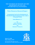
1
IMPROVING FLOW DISTRIBUTION IN SMALL-SCALE WATER-SUPPLY SYSTEMS THROUGH THE USE OF FLOW-REDUCING DISCS AND METHODS FOR ANALYZING THE EFFECTIVENESS OF SOLAR POWERED PUMPING FOR A DRINKING WATER SUPPLY IN RURAL PANAMA By Briana I. Drake A REPORT Submitted in partial fulfillment of the requirements for the degree of MASTER OF SCIENCE In Environmental Engineering MICHIGAN TECHNOLOGICAL UNIVERSITY 2015 ©2015 Briana I. Drake This report has been approved in partial fulfillment of the requirements for the Degree of MASTER OF SCIENCE in Environmental Engineering. Civil and Environmental Engineering Department: Report Advisor: John S. Gierke Committee Member: Brian D. Barkdoll Committee Member: Leonard J. Bohmann Department Chair: David W. Hand Table of Contents Table of Figures .................................................................................................................................... v Table of Tables ..................................................................................................................................... v Abstract.................................................................................................................................................. 1 1.0 Introduction .................................................................................................................................... 2 1.1 Project Motivation ..................................................................................................................... 3 1.2 Objectives ................................................................................................................................... 3 2.0 Project Site: Guayabo, Coclé, Panamá (8°50'35"N, 80°21'48"W) .......................................... 5 2.1 Rural Water Supply in Panama ................................................................................................ 6 2.2 Water in Guayabo ...................................................................................................................... 7 3.0 Methods: Solar Pumping System ................................................................................................. 8 3.1 Components of a solar pumping system ................................................................................ 8 Pump .............................................................................................................................................. 9 Solar Panels .................................................................................................................................10 Storage Tank ...............................................................................................................................10 Battery ..........................................................................................................................................11 Other considerations .................................................................................................................11 3.2 Evaluating the Efficiency of a Solar Powered Pumping System ......................................11 3.2a Solar Efficiency ......................................................................................................................13 3.2b Pump Test Data Collection .................................................................................................14 Pumping Head ............................................................................................................................15 Pump Efficiency.........................................................................................................................15 4.0 Methods: Flow-Reducing Discs .................................................................................................16 4.1 NeatWork Model Calibration ................................................................................................17 4.2 Evaluation of Loss Coefficient with Multiple Open Spigots ............................................19 4.3 Use of a Single Sized Flow-Reducing Disc ..........................................................................19 5.0 Results & Discussion ...................................................................................................................20 5.1 Solar Pump Test Analysis .......................................................................................................20 5.2 Modes of Failure of Solar Pumping Systems.......................................................................24 5.3 NeatWork Model Calibration ................................................................................................25 5.4 Use of a Single Sized Flow-Reducing Disc ..........................................................................28 6.0 Future Work .................................................................................................................................30 7.0 Conclusions...................................................................................................................................30 iii References ...........................................................................................................................................32 Appendix A: Construction of a Water Level Sounder..................................................................33 Appendix B: Fabrication of Flow-Reducing Discs .......................................................................35 Appendix C: Example Single Flow Reducer NeatWork Simulation Outputs...........................36 iv Table of Figures Figure 1: Location of Guayabo, Panama (Source: Google Maps) ................................................ 5 Figure 2: Location of Guayabo, Panama in relation to the Toabre and Tulu Rivers (Source: Google Maps) ....................................................................................................................................... 5 Figure 3: Sombrero Pintado made in Guayabo, Panama ............................................................... 6 Figure 4: Hand dug well in Guayabo, Panama................................................................................. 7 Figure 5: Flow-reducing discs ............................................................................................................. 8 Figure 6: Schematic of a solar pumping system ............................................................................... 9 Figure 7: Comparison of solar irradiance and pumping rate for a Grundfos 11SQF-2 helical rotor solar pump in Caimital, Panama over a 40 minute period. ................................................10 Figure 8: Installation options for flow-reducing discs before household connections............17 Figure 9: Pressure drop measurement setup ..................................................................................19 Figure 10: Solar pumping set-up at Gierke Blueberry Farm, September 2014 .........................21 Figure 11: Solar pumping drawdown not limited by solar intensity at Gierke Blueberry Farm ...............................................................................................................................................................21 Figure 12: Pumping test during variable sunlight intensity at Gierke Blueberry Farm ............22 Figure 13: Pump curve comparison with measured data. Partially recreated from (Grundfos Pumps Corporation, 2011)................................................................................................................24 Figure 14: Comparison of NeatWork modeled flow rates using an orifice coefficient of 0.59 and 0.68 to those measured in Guayabo, Panama.........................................................................27 Figure 15: Comparison of Modeled and Measured Flow Rates with Multiple Open Spigots 28 Figure 16: Frequency of average flow rates in the community of Limon as modeled in NeatWork with varying selections of flow-reducing discs ...........................................................29 Figure 17: Homemade water level sounder with detail of the circuit connection ....................34 Table of Tables Table 1: NeatWork inputs and outputs...........................................................................................16 Table 2: Weather station solar data for calculation of solar panel efficiency in Chassell, Michigan on September 26, 2014.....................................................................................................22 Table 3: Measured power draw for calculation of solar panel efficiency in Chassell, Michigan on September 26, 2014 ......................................................................................................................23 Table 4: Determination of the optimum NeatWork orifice loss coefficient (θ) .......................26 Table 5: Analysis of ideal single sized flow-reducing disc on a variety of water systems ........29 Table 6: Determination of ideal single-size FRD based on elevation variations on a single community...........................................................................................................................................30 v Abstract As continued global funding and coordination are allocated toward the improvement of access to safe sources of drinking water, alternative solutions may be necessary to expand implementation to remote communities. This report evaluates two technologies used in a small water distribution system in a mountainous region of Panama; solar powered pumping and flow-reducing discs. The two parts of the system function independently, but were both chosen for their ability to mitigate unique issues in the community. The design program NeatWork and flow-reducing discs were evaluated because they are tools taught to Peace Corps Volunteers in Panama. Even when ample water is available, mountainous terrains affect the pressure available throughout a water distribution system. Since the static head in the system only varies with the height of water in the tank, frictional losses from pipes and fittings must be exploited to balance out the inequalities caused by the uneven terrain. Reducing the maximum allowable flow to connections through the installation of flow-reducing discs can help to retain enough residual pressure in the main distribution lines to provide reliable service to all connections. NeatWork was calibrated to measured flow rates by changing the orifice coefficient (θ), resulting in a value of 0.68, which is 10-15% higher than typical values for manufactured flow-reducing discs. NeatWork was used to model various system configurations to determine if a single-sized flow-reducing disc could provide equitable flow rates throughout an entire system. There is a strong correlation between the optimum single-sized flowreducing disc and the average elevation change throughout a water distribution system; the larger the elevation change across the system, the smaller the recommended uniform orifice size. Renewable energy can jump the infrastructure gap and provide basic services at a fraction of the cost and time required to install transmission lines. Methods for the assessment of solar powered pumping systems as a means for rural water supply are presented and assessed. It was determined that manufacturer provided product specifications can be used to appropriately design a solar pumping system, but care must be taken to ensure that sufficient water can be provided to the system despite variations in solar intensity. 1 1.0 Introduction In 2000, the World Health Organization (WHO) set out to create a set of Millennium Development Goals (MDGs) to address health, equality, safety and human rights in some of the world's poorest regions. With the goal year 2015 upon us, it is an appropriate time to acknowledge the work completed and reassess strategies for moving forward with the work that still remains. The MDG target 7C addresses water and sanitation: to halve, between 1990 and 2015, "the proportion of the population without sustainable access to safe drinking water and basic sanitation" (Bartram et al., 2014). The WHO reports 89% worldwide access to an "improved" water source where "improved" is defined as access to a public tap, borehole, protected spring, rainwater collection system, bottled water from an "improved" source, or piped water into the dwelling (World Health Organization and United Nations Children's Fund, 2014). Panama has a bustling economy that has been steadily growing since the Panamanian government took control of the Panama Canal in 2000. The skyline in Panama City resembles something close to Miami with a smattering of skyscrapers lined up along the oceanfront. Though this wealth is not equally distributed throughout the country. Overall 37% of the country lives in poverty, including 54% of all rural residents and 98% of people living in indigenous regions (Oficina de Naciones Unidos de Panama, 2015). This economic disparity is exacerbated by the lack of public infrastructure connecting these rural communities. Often times there is no grid electricity and many only have access to seasonal roads. With a rainy season that lasts eight months, the only way to travel to these communities for the majority of the year is by foot or horse. Though the Ministry of Health is responsible for building and overseeing rural water systems, their staff is overworked, under trained, and financially strapped. Even when ample water is available, mountainous terrain significantly affects the pressure available throughout a water distribution system. Static pressure variances in a system will only fluctuate with the height of water in the tank. Frictional losses from pipes and fittings must be understood and controlled to balance flows and pressures at individual connections, or taps, across the uneven terrain. The use of distribution-system grids can increase flow equality in a system (Chandapillai, Sudheer, & Saseendran, 2012), but in many rural settings, houses are built far apart on slopes where a branching network is the most feasible choice. Reducing the maximum allowable flow to connections through the installation of flowreducing discs can help to retain enough residual pressure in the main distribution lines to provide reliable service to all connections. The use of renewable energy is growing throughout the world. Since the 1990s, development investors have increased international funding for off-grid applications (Biomass Users Network, 2002). In a development context, renewable energies can jump the infrastructure gap and provide basic services at a fraction of the cost and time required to install transmission lines. Just like many countries have seen the rapid expansion of cellular telephone networks reaching more remote areas without the infrastructure costs of installing many miles of telephone wires, people in even the most remote areas can use solar 2 panels to produce their own electricity which can be used for multiple purposes including, as in this context, the pumping of water for household consumption. This report evaluates two independently functioning parts of a water distribution system in rural Panama that includes the use of flow-reducing discs to mitigate flow inequalities. It also reviews methods for the assessment of solar powered pumping systems as a means for rural water supply. 1.1 Project Motivation While serving as an Environmental Health volunteer with the Peace Corps in Panama, I supported several communities with the analysis, construction and maintenance of their water systems. I lived and worked in a rural community where I experienced dry-season water shortages, struggled to facilitate community decisions regarding their water system, and joined with my neighbors to fix pipeline breaks. Peace Corps Panama trained me in the use of the NeatWork program for the design and analysis of water distribution systems. The community of Guayabo, in the province of Coclé, is accessed by a twice-daily 2-hour truck ride from the regional capital of Penonomé, followed by an hour hike. The mountainous region had limited access to materials, transportation, grid electricity, formal education and financial resources. More details on the project location are included in Section 3.0. Though the majority of rural water systems in Panama are gravity fed from natural springs (Suzuki, 2010), the community of Guayabo presented a unique challenge in that part of the community, including the church and school, was located above the highest spring in the area requiring community members to haul water out of a hand dug well and carry it to these locations. Like in many mountainous communities, flow equality throughout the water system proved troublesome. The need for an effective and affordable solution to this inequality drove me to investigate the effectiveness of a technique Peace Corps Panama uses, handmade flowreducing discs. Though separate technologies, I chose to look at both solar powered pumping and flow-reducing discs because of their applicability in the community of Guayabo. 1.2 Objectives As efforts are made to expand improved water sources to an increasing number of communities, technologies must be adapted to meet the unique needs of these settings. Flow-reducing discs and solar pumping are two examples of technologies that can be employed when conventional systems are not appropriate for small rural communities. Objective 1: Calibrate the NeatWork model and use it to determine the appropriate flow-reducing disc sizes that provide equitable flows across communities with varying elevation gradients. Elevation variations throughout small water systems can produce severe flow inequalities to individual connections. Regulating the system by decreasing frictional losses through the 3 installation of dramatically larger pipe sizes to trouble prone locations can be cost prohibitive, but flow-reducing discs present a cost effective solution to these inequalities. Although models are available to simulate branched distribution systems with flow-reducing discs, many practical applications in low-resource settings make sophisticated analyses problematic. This report aims to calibrate the NeatWork model to produce measured flows. A sub objective of this work is to ascertain the feasibility and effectiveness of using a singlesize of flow-reducing disc throughout an entire water system and if this size can be determined based solely on the elevation variation in the community. Objective 2: Evaluate solar-powered pumping performance relative to manufacturer specifications and engineering design principles. As countries and non-governmental organizations (NGOs) continue to expand water and sanitation infrastructure to the most remote reaches of their countries, they face larger issues of first providing the necessary infrastructure to support their projects. The use of solar technology allows water and sanitation projects to leapfrog more expensive and involved electrification and transportation projects. Data on in situ performance of solar-powered systems is not prevalent in water-supply development literature and water-system managers must rely only on manufacturers’ literature. This work will demonstrate approaches appropriate to measure performance and the observed performance compared to manufacturer performance specifications. 4 2.0 Project Site: Guayabo, Coclé, Panamá (8°50'35"N, 80°21'48"W) Guayabo is a small community of 200 people on the north side of Panama's central mountain range. The community is at the top of a river valley 75 kilometers north of Coclé's regional capital of Penonomé. Though relatively close geographically, a lack of adequate infrastructure leaves the community accessible only by foot or horse for the majority of the year. Figure 1: Location of Guayabo, Panama (Source: Google Maps) Figure 2: Location of Guayabo, Panama in relation to the Toabre and Tulu Rivers (Source: Google Maps) 5 The majority of families in Guayabo make a living as subsistence farmers who earn extra income by weaving sombreros pintados. These sombreros are a staple accompaniment to traditional Panamanian dress. Palm leaves are harvested, boiled, cut and dried before being weaved into long strips that are then stitched together using a natural fiber called pita. Each hat takes about two weeks to weave and is sold for between US$35 and US$70 depending on the quality. Figure 3: Sombrero Pintado made in Guayabo, Panama Rice is a staple of the Panamanian diet and is also a widely cultivated crop in the region. Other common crops include yucca, corn, bananas, and coffee. Crops are generally just grown for household consumption. The only full time paid positions in Guayabo are the elementary school teacher and health post assistant who is responsible for monitoring vaccinations, infant weight and providing general medical assistance for Guayabo and several surrounding communities. Many people take temporary positions outside of the community working construction, as nannies, hotel staff, and mining gold near Coclesito. Working family members typically leave for a week or two and then return to Guayabo for a few days before returning again to work. 2.1 Rural Water Supply in Panama Many rural communities in Panama depend on spring sources for their drinking water. Flowing freely from the ground, these springs are collected with a concrete damming structure and the collected water is then conveyed by gravity to the community storage tank. This type of system is economical to implement, totaling US$7000 for a standard system 6 serving about 500 people. These systems are relatively straightforward to maintain due to the lack of mechanical parts. When an adequate spring source is not available at an elevation higher than the community buildings, a pump must be used to elevate the water to a storage tank. Many rural communities are still not connected with a paved road or grid electricity which limits their options for affordable and accessible electricity. If there is a pump in place, it is typically powered by a gasoline generator. The travel time and expense to purchase and then transport gasoline for the system is typically cost prohibitive so they are generally run sporadically. Not only is fuel expensive and difficult to obtain, hydrocarbon combustion contributes to the production of green house gases. Renewable energy sources, though requiring a large initial investment, present a solution to the majority of these issues. Most importantly, they create energy from a locally available source. 2.2 Water in Guayabo The Toabre River provides strong flows throughout the year, but it is a 30-minute muddy hike downhill from the community center. Part of Guayabo receives water from a natural spring that fills a storage tank and is then piped to a few nearby homes. There is a section of town that was constructed at too high of an elevation to receive water from this system and has thus been pulling water from a hand dug well and carrying it to the church, school and multiple homes. Figure 4: Hand dug well in Guayabo, Panama 7 Through a grant from the Energy Climate and Partnership for the Americas, funding through the Peace Corps Partnership Program and coordination with a Panamanian solar contractor, a solar pumping system was installed in the existing hand-dug well to transfer water to two tanks installed at the school, the highest connection served by the system. The tanks ensure water availability throughout the day as the pump will only function during sunlight hours. The pumping system consists of four 85-Watt monocrystalline silicon solar panels (ET Solar Industry Limited, Taizhou, China) installed in series to provide a total of 380 Watts at 48 VDC to the controller box where the electricity is converted from DC to AC to run the Lorentz PS600-HR07 helical rotor pump (Henstedt-Ulzburg, Germany). The panels were installed horizontal, due to the near-equatorial latitude of the community. The pump is controlled by a level control float switch (Lorentz, Henstedt-Ulzburg, Germany) installed in the water storage tank eliminates tank overflow. The well’s large diameter allows room for the pump while still leaving space to draw water by hand with a rope-and-bucket in case the pump breaks or does not function for lack of sunlight. The distribution system uses minimally sized pipes to reduce the cost required for construction. Handmade flow-reducing discs from flattened PVC pipe are installed before individual connections to regulate pressure inequalities, caused by mountainous terrain. Figure 5: Flow-reducing discs 3.0 Methods: Solar Pumping System As the price of solar panels continually drops and the efficiency increases, solar becomes an increasingly more practical energy source for rural areas without grid electricity. Solar panels eliminate the monetary expense and logistical burden of purchasing fossil fuels as well as the environmental impacts of burning fossil fuels. With a demonstrated lifespan of 40 years and an average cost of US$1/Watt (Bazilian et al., 2013), solar panels are becoming an increasingly more viable energy source in developing communities. 3.1 Components of a solar pumping system A solar pumping system generally consists of the panels, a control box that may also be a DC/AC power inverter, and the pump. The design of a pumping system is a heuristic process. There are usually factors that limit availability, such as the lift height or the aquifer yield. System components are chosen to best meet the flow demands in accordance with the 8 limiting factors.. Limiting factors could include the quantity of water available in the well due to a slow recharge rge rate, community water demand, or the cost of the system. It is most ideal to design a system starting from the water demand of the community, but this is not always economically feasible. Figure 6: Schematic of a solar pumping system Pump Unlike conventional fixed--speed speed pumps with a constant energy source, solar pumps are required to work over a wide power-input range, dependent nt on variable solar intensity. Slight variations in sunlight ght intensity and cloud cover cause pumpin pumpingg rates to deviate from ideal conditions. Figure 7 shows the comparison between solar irradiance and pumping rate for a Grundfos 11SQF-22 helical rotor solar pump (Bjerringbro, Denmark). 9 7.0 6.5 6.0 5.5 Solar Irradiance Flowrate 5.0 4.5 Flowrate (gallons/minute) Solar Irradiance (W/m2) Grundfos 11SQF-2 Helical Rotor Solar Pump 900 800 700 600 500 400 300 200 100 0 11:40 AM 4.0 11:50 AM 12:00 PM Time 12:10 PM 12:20 PM Figure 7: Comparison of solar irradiance and pumping rate for a Grundfos 11SQF-2 helical rotor solar pump in Caimital, Panama over a 40 minute period. Solar pumps are generally either helical rotor (positive displacement) or multi-stage centrifugal styles. Helical rotor pumps can provide water at an increased head where centrifugal pumps can produce higher flow rates. Specific manufacturers will provide the power requirements, maximum achievable lift, and maximum flow rate specifications for each pump available. Grundfos (www.grundfos.com) and Lorentz (www.lorentz.de) are leading manufacturers of solar powered drinking water pumps. A standard pump curve compares the output as flow to the total dynamic head (TDH). The assumption is that the power supply can be met for the pump chosen and it is known how the pump will perform at a given TDH. With a solar pump, the power supply is the independent variable upon which the output is dependent for a given TDH. Solar Panels The solar array is designed to meet the pump's power requirements. System voltage varies depending on whether the panels are configured in series (voltage is additive) or parallel (voltage is uniform). Determining the solar array configuration will depend on the nominal voltage requirements of the pump. Electrical current (amperage) will vary with different configurations and pump speed (power draw). The input power is the product of the voltage and amperage. Panels are rated on their ability to produce Watts per hour (W) and their efficiency is accounted for in the manufacturer's listed rating. The cheapest and most effective way to increase pumping performance is to over design the solar array capacity. The electricity generation ratings are determined from optimal sunlight conditions which are unreasonable to expect on a daily basis. By over sizing the solar array, the minimum power required to run the pump is more likely to be achieved at times of weaker solar irradiance. Storage Tank The majority of water for a system is consumed during certain peak-demand hours of the day, mostly in the morning. In the morning, families use water to cook breakfast, bathe, and 10 wash laundry. However, little or no sunlight is available at this time to run the pump. In order to meet the morning demand, a system must also include either a water storage tank or a battery. The storage tank can be filled during peak sunlight hours and be consumed by households as needed. A battery stores excess energy, allowing the pump to be run at any time, day or night, that water is desired from the well. The size of the tank is dependent on the community water demand. For example, through household surveys in her community, a volunteer determined that her community of 50 people requires 1,100 gallons of water a day and they use about 52% of that water between 6-9 am. Thus the tank would be sized at a minimum of 600 gallons to provide the desired water in the morning before sustained solar pumping can occur. Information on the design and construction of the actual tank is outlined in Chapter 14 of the Field Guide to Environmental Engineering for Development Workers (Mihelcic et al., 2009). Battery Batteries increase the flexibility of the system by allowing the pump to run independent of sunlight but also increase the system cost. Generally, several batteries must be installed in series to achieve the same nominal voltage requirements of the pump. For example, if a pump has a nominal voltage requirement of about 48 VDC, four 12-VDC batteries connected in series would be required to obtain the minimum voltage. A housing structure must also be constructed near the panels and pump to keep the batteries dry, cool and protected. Batteries must be secured as valuable and vulnerable parts of the system. Other considerations A low water shut off sensor protects the pump from damage as the water source runs dry. Some pumps have this feature built in, but for other pumps it must be purchased separately and installed. The amount of water available in a well can be determined based on storage and recharge rate, and this can be used to predict the maximum production of the well. A level-controlled float switch is a sensor installed in the tank that stops the pump from running when the tank is full. This allows extra water to be stored in the well and eliminates overflow at the tank. Between the panels and the pump, the electricity passes through a controller box. This varies for every system, ranging from a simple switch box to a conduit to connect the above mentioned low water shut off sensor and level controlled float switch. It will also act as an inverter if the pump runs on AC electricity. Some pumps allow the maximum operating speed to be manually adjusted which will limit the pump speed from changing too dramatically as solar intensity varies. There are also a few models that can be connected to a diesel generator through the control box which can be a good alternative for low sunlight times such as the rainy season. 3.2 Evaluating the Efficiency of a Solar Powered Pumping System Solar powered pumping systems are designed based on the specific site needs and the pump manufacturer's listed specifications. Environmental conditions are a major factor in the 11 performance of a solar system as variances in solar intensity are directly correlated to the pumping rate and thus the amount of water available to the community. The following will provide a guide to assessing the performance of the well, solar panels, and pump in a given system. The following assessments are described in further detail in the subsequent subsections. Information to collect and consider includes: Several measurements taken in the field will be necessary to compile a complete analysis of the solar pumping system. 1. Depth of well and depth to water The depth to the water level in the well can be measured using a water level sounder or by simply lowering an object on a string and measuring the length of the string. It is important to measure depth to water throughout the year to account for seasonal variations in the water table. The depth of the well itself can be obtained from drilling logs. The depth of the pump can be determined from the length of pipe installed above the pump. Hand dug wells have limited depth below the water table due to the infeasibility of digging underwater. 2. Diameter of the well Knowing the depth of the well and the diameter, the storage in the well can be calculated and specifically the volume of water stored in the well above the pump. Depending on the recharge rate of the well, the water storage capacity of the well cavity itself may be significant to the amount of available water to the system. 3. Height above ground to the tank and distance of tubing Record the size, rating and length of all pipes installed between the pump and the tank. These measurements will be required to determine frictional losses as they contribute to the total dynamic head (TDH). The height difference between the well head and the tank inlet will also need to be measured. This can be done with an Abney level if available or a simple water level device. 4. Well Recharge Rate The productivity of a well is determined by running a pump test and measuring the level of water in the well in conjunction with the amount of water being removed from the well. After the water level draws down to an equilibrium depth, the pump can be shut off and then the depth to the water table is measured as a function of the time it takes for the water table to return to its original level. Section 4.2b provides more in depth information on the collection of data for a pumping test. 5. Well configuration The possibility of excessive sediment loading in a hand-dug well should be 12 considered as this may contribute to failure of the pump. Hand-dug wells often times do not allow for much more than 10 feet of standing water. This may become an issue depending on the net positive suction head requirements of your pump and how critical the borehole storage is if the aquifer has a slow recharge rate. 6. Daily water demand of the community The community water demand can be determined by conducting household water use surveys or is often times estimated by public health organizations. Panama's Ministry of Health recommends 30 gallons of water per person per day for communities using latrines for sanitation (Gobierno Nacional República de Panamá, 2010). This has been found in practice to be higher than actual water demands. 3.2a Solar Efficiency The efficiency of solar panels is a measure of how much electricity can be produced per square meter of panel. More efficient solar panels can produce the same amount of electricity from a smaller surface area. The most efficient commercially available solar panel modules are currently 25% efficient (National Renewable Energy Laboratory, 2014). Efficiency is traded off for cost, so more affordable panels do not reach this efficiency. Measure concurrently: a. Solar Irradiance (W/m2) b. Volts c. Amps Equipment used for data collection includes: • • DS-05A solar irradiance meter manufactured by Daystar, Inc. of New Mexico ($157). Measures solar irradiance in Watts per cubic meter (W/m2). The meter has ±3% accuracy from 0-1200 W/m2 (Daystar Inc., 2014). CM100 AC/DC Low Current Clamp Meter. Manufactured by General Technologies Corporation (GTC), Canada ($143). Measures the DC volts provided by the solar array and the AC current drawn by the pump. Data Collection Procedure The process for collecting solar system data is as follows: 1. Simultaneously measure solar irradiance with volts and then amps. 2. The Daystar solar irradiance meter will be held along the side of the array, facing the sky at the same angle as the panels. As the display varies rapidly, an average will be taken. Data will be recorded in Watts/m2. 3. Volts will be measured in DC by connecting the positive and negative probe ends to appropriate negative and positive wire connections within the control box. 13 4. Amps will be then be measured on the AC setting, as they are converted in the controller before being sent to run the pump, utilizing the clamp feature of the ammeter around one of the wires running to the pump. Efficiency is then calculated as the amount of electricity generated per area as compared to the solar potential available. = ݕ݂݂ܿ݊݁݅ܿ݅ܧ ݎ݁ݓ ݐݑݐݑሺܸ ∗ ܣሻ ܹ ݁ܿ݊ܽ݅݀ܽݎݎ݅ ݎ݈ܽݏቀ ଶ ቁ ∗ ܽ݁ݎܽ ݈݁݊ܽሺ݉ଶ ሻ ݉ (1) 3.2b Pump Test Data Collection A pump test will help to determine aquifer characteristics as well as pump function under varying solar conditions. Measuring the solar irradiance in line with the pumping rate can help to determine how solar variations affect the water available in the system. Measuring the well recharge rate, or how fast water from the surrounding aquifer enters the well, determines the available water during continued pumping. Equipment used for data collection includes: • • • • Homemade water level meter or sounder (Construction details in Appendix A: Construction of a Water Level Sounder(Government of Alberta, 2014)) Stopwatch 5-gallon bucket 15 PSI pressure gauge, WIKA with 1/4" NPT connection Data Collection Procedure These steps will be followed for the collection of drawdown and recharge measurements: 1. Let the well sit undisturbed for 12 hours prior to the pump test to allow the static water level to stabilize. 2. Measure the static water level with the sounder. 3. Turn the controller box on and pumping will begin when there is sufficient sunlight to start the pump (around 9:30am for the test site). 4. Flow rates will be measured at the tank by measuring the time to fill a 5 gallon bucket. They will be measured every 10 minutes. 5. The sounder will be raised up about 6 inches between readings and once every 10 minutes will be lowered down slowly until the circuit is connected, sounding the siren. The depth will be recorded to the closest tenth of an inch. 6. Extent of pumping will likely be dictated by the solar intensity and may have gaps due to cloud cover or need to be stopped early in the case of rain. 7. Depth to water will be measured with the sounder once every 10 minutes for the first hour once pumping has finished and recharge has begun. After the first hour, depth will be recorded once every 30 minutes. This frequency will increase for smaller diameter wells. 14 Pumping Head Pumping head or total dynamic head (TDH) is the amount of pressure the pump is required to overcome to get water from a well into a tank, as expressed as a height of water. This height includes the actual lift between the well and the tank, but also factors in frictional losses from the pipes and fittings. When choosing a pump, the TDH will be a necessary parameter to consider. The following equation can be used to determine frictional losses from the pipe walls (Mihelcic et al., 2009). ℎ = 16݂ ܳܮଶ 2݃ߨ ଶ ܦହ (2) Where hL is the frictional head loss (feet), L is the length of pipe (feet), Q is the flow rate (ft3/sec), g is gravity (32.8 ft/s2) and D is the diameter of the pipe (feet). The frictional factor, f=ks/D. ks for PVC = 3.3x10⁻⁷ and the diameter of tubing from the pump to the tank is 1.25" or 0.104 ft. This ks/D value corresponds to a friction factor of 0.008. Pump Efficiency Energy losses originate from inefficiencies in the panels, the current converter and the pump itself. These all contribute to the overall efficiency of the system. Solar pump efficiency is said to be between 40% and 60% and can be calculated using flow rates and solar power outputs and the following equation (LORENTZ, 2010): ݕ݂݂ܿ݊݁݅ܿ݅ܧሺ%ሻ = ܸ݁ ݐ݂݅ܮ ݈ܽܿ݅ݐݎሺ݂ݐሻ ∗ ݓ݈ܨሺܯܲܩሻ ∗ 18.8 ܲ ݎ݁ݓሺܹሻ Assuming: 1 Horsepower = 33,000 ft*lb/min 1 Horsepower = 750 Watts 1 ft3 = 7.48 gallons of water Unit weight of water = 0.000161 ft3/lb 15 (3) 4.0 Methods: Flow-Reducing Discs Water distribution systems in Panama's rural, mountainous communities present large static pressure inequalities at homes throughout the system from elevation variations of up to 100 meters. Homes at lower elevations generally receive adequate flow rates, but pressure losses from open or broken spigots and broken pipes cause those at higher elevations to suffer from a lack of residual pressure in the main line required to lift the water to their spigots. Water system design programs such as EPANET (Rossman, 2000) often mitigate these differences in flow inequality by raising the height of the tank to increase overall system pressure and increasing pipe diameters to reduce frictional losses. This can be replicated by creating artificially high head losses at the high flow houses in order to maintain more residual pressure in the system. Flow-reducing discs (FRD) cut from flattened PVC piping with a hole saw can cheaply and easily reproduce this extra frictional loss. The fabrication of flow-reducing discs is outlined in Appendix B. Flow-reducing discs sizes were designed using NeatWork (www.neatwork.ordecsys.com), a free software program created by the non-governmental organization Aqua para la Vida and the University of Geneva, specifically for the design of water distribution systems in rural areas (Agua Para la Vida, 2002). The program is used by the Environmental Health sector of Peace Corps Panama to design and analyze water systems where volunteers live and work. NeatWork optimizes performance while minimizing cost by regulating flow inequalities with flow-reducing discs as opposed to widely varying pipe sizes. NeatWork has a rougher user interface than EPANET as it is Java based and has no spatial mapping component. The program's required inputs and its outputs along with its capabilities are listed in Table 1. Table 1: NeatWork inputs and outputs Inputs Outputs • Nodes: All fittings, changes in pipe size and faucets are marked by a node that is defined by its height in meters below the tank which is a node itself at a height of 0 meters. • Arc Lengths: Arcs are the sections connecting all of the nodes. Their length is entered in meters. • Available Materials: Choose the size and rating of PVC pipes available for purchase and the size of FRDs available which may simply correlate to the size of drill bits. • Target flow rate at faucets in liters/second • Several other parameters can be customized including the coefficient used to calculate the headloss created by the FRD and the fraction of simultaneously open faucets. • Pipes Sizes: in meters for the entire system. • Orifice Sizes: for flow-reducing discs. Diameter in meters. • Simulations produce: Flow at nodes (liters/second) Speed in pipes (meters/second) Head pressure at nodes (meters) Percentiles of maximum flows • Ability to customize designs after they have been created and run simulations on new iterations. 16 NeatWork is capable of running Monte Carlo sampling for a user defined percentage of open faucets over the entire system. It also performs simulations for a single open faucet or a user-defined set of faucets simultaneously. Further explanation on the use of the program is provided in the user's manual (Agua Para la Vida, 2002). Economic Advantage The equalization of flow in a system through the installation of large-diameter pipe sizes can be cost prohibitive. For example, in the design for one rural community, NeatWork, designing without flow-reducing discs, suggested 4" PVC piping for a 50-foot uphill stretch to a home, which at US$50.00 per 20-foot section would cost US$125.00. If using flowreducing discs, the same house could be connected using a 3/4" pipe for US$18.50 (US$6.00 per 20 foot section). The installation of flow-reducing discs can, for just this one house, produce a savings in excess of US$100. In an area where the average monthly income is less than US$200 per family, cost differentials of that size can be cost prohibitive for the project. When the correct materials cannot be purchased for a project, flow inequalities will remain. Installation The FRDs were installed on the pipes after the main line that head to individual connections before the spigots, glued in place where two pipes connect or in this case, before a shut off valve for the individual connection. The ball valves were only in place to turn off water to a connection in the case of truant water payments or system maintenance. The valves were not used to regulate flow. from Mainline to Spigot Figure 8: Installation options for flow-reducing discs before household connections 4.1 NeatWork Model Calibration Simulations were conducted within NeatWork using a range of coefficients (ߠ) to determine which most closely reproduced the flow rates measured in the field. 17 NeatWork uses the following equation to calculate flow reducer size (Agua Para la Vida, 2002). ߲ℎ = −ߠ ܳଶ ݀ସ Where, ߲ℎ = the head loss across the orifice (m) ܳ = flow rate (m3/s) d = diameter of the orifice (m) ߠ = is the choice of the designer. (4) The coefficients (ߠ) will vary based on the construction of the discs. The original coefficients were determined in the lab using manufactured FRDs with a guaranteed diameter. The following procedure was used to measure flow rates that were used in the calibration process. Equipment Used: • Two 15 PSI pressure gauge, WIKA with 1/4" NPT connection • Various sizes of homemade flow-reducing discs • PVC ball valve to mimic the way the flow-reducing discs were installed in shutoff valves before each faucet • Stopwatch • 5-gallon bucket Data Collection Procedure: 1. Measuring setup, as depicted in Figure 9, was installed, with the desired flowreducing disc placed before the ball valve. 2. An initial pressure reading was recorded with the spigot closed if it was less than 15 psi. 3. With the spigot completely open, the time to fill a 5-gallon bucket was measured. 4. Pressure readings before and after the FRD were recorded while the spigot was open. The rest of the distribution system was completely closed except for the spigot being measured. 18 Figure 9: Pressure drop measurement setup 4.2 Evaluation of Loss Coefficient with Multiple Open Spigots The flow rate at a single open spigot is very predictable and easily calculated with data on the system characteristics. The system is less easy to predict when multiple spigots are open at the same time. Modeling the flow at concurrently open spigots produces results that are more likely to resemble real life situations within the system. Several flow rates were measured concurrently in the field to compare to modeled data. Data Collection Procedure: Simultaneous flow of 3 open spigots 1. A whistle was used to signal the measurers at each separate connection. The whistle was blown once and all spigots were opened. 2. The whistle was blown a second time and all 3 parties started measuring the time to fill a 5 gallon bucket. They hollered in when their bucket was full, but left their spigot open. 3. The whistle was blown once more and all spigots were closed and results were recorded. Concurrent flow data to match the measured data sets was modeled in NeatWork using the predetermined orifice coefficient value as well as the optimum coefficient as determined by the manipulation of the model with individual faucet flows. 4.3 Use of a Single Sized Flow-Reducing Disc Installing appropriately sized flow-reducing discs improves flow equality throughout a distribution system, but requires detailed elevation surveys and computer design experience in order to determine the appropriate FRD sizes. Determining if a single size of FRD can be used throughout an entire distribution system to equalize flow rates would enable communities, without the capability to conduct detailed surveys or use computer design programs, to employ FRDs in their distribution system. 19 A distribution system with flow-reducing discs is optimized when both the pipe sizes and flow-reducing discs are designed and installed from scratch. Once FRDs are installed, they cannot be removed without cutting the pipe around them. Installing a single-sized flowreducing disc throughout an entire system creates transparency for the assessment of the distribution system and increases the ease of connecting new houses to the system by requiring inventory of only one size of disc. When choosing a single size of FRD for a system, a smaller orifice will always reduce variability in flow rates found throughout the system, but can also unnecessarily restrict flows. The objective is to choose a FRD size that eliminates insufficient flows while keeping the average flow rate as high as possible. Methods: After calibrating the NeatWork model to simulate measured flows, multiple simulations were run on a variety of systems to determine the single size of FRD that produced the optimum flow equality throughout the entire system. This determination was made by eliminating FRDs that created flows of less than 1.6 gpm to any connection. If there are multiple single FRD sizes that achieve this for a given system, the system with the highest average flow rate is chosen to avoid unnecessarily constriction of water supply. 5.0 Results & Discussion As water enters the tank from the pump, the system resets to atmospheric pressure so the two halves of the system, pumping and distribution, operate independently of each other. The results are separated for the two systems. 5.1 Solar Pump Test Analysis Due to incomplete data sets from the project location, example data from Michigan was used to calculate all values and graphs as outlined in the Section 4. Pumping tests were conducted at Gierke Blueberry Farm in Chassell, Michigan in the fall of 2014 to produce example data. The farm utilizes a Grundfos 16 SQF-10 (Bjerringbro, Denmark) 10-stage centrifugal pump directly off of 1470 Watts of solar panels (6 X 245W in series) (Towards Excellence, Taizhou, China). The pump is set up for irrigation but for testing purposes, flow rates were measured at the well head. Slightly different equipment was used for data collection because of the location of the testing: • • • • Hobolink weather station - solar, temperature, barometric pressure (Data available at: https://www.hobolink.com/p/47316a1a1d140ad082139599206946ab) (Onset Computer Corporation, Bourne, MA) Solinst Levelogger - Model 3001 Edge (Georgetown, Ontario, Canada) 5 gallon bucket and stopwatch Solinst Water Level Sounder (Georgetown, Ontario, Canada) 20 Figure 10: Solar pumping set-up at Gierke Blueberry Farm, September 2014 As stated in Section 4.0, pumping rates are highly dependent on solar intensity. This means that pumping tests do not always mimic standard pumping tests with a clear drawdown to equilibrium and recovery period, especially during times of varying solar intensity. Solar Puming Test at Gierke Blueberry Farm September 26, 2014 Depth to Water Level (m) 8:00 AM 12 10:00 AM 12:00 PM Time 2:00 PM 4:00 PM 6:00 PM 14 16 18 20 22 24 26 28 30 Figure 11: Solar pumping drawdown not limited by solar intensity at Gierke Blueberry Farm Figure 11 is an example of a solar powered pumping test that is not limited by the solar intensity. In strong sunlight conditions, the pump can run consistently at its highest flow rate and is only limited by the recharge rate of the water source which dictates the water level. 21 Solar Puming Test at Gierke Blueberry Farm October 9, 2014 5:00 AM 12 7:00 AM 9:00 AM Time 11:00 AM 1:00 PM 3:00 PM Depth to WL (m) 14 16 18 20 22 24 26 28 30 Figure 12: Pumping test during variable sunlight intensity at Gierke Blueberry Farm Figure 12 shows a pumping test during a period of solar variance which is characterized by fluctuations in the pumping rate. These fluctuations are visible in the depth to water level. As the pumping rate becomes slower than the recharge rate of the aquifer, the water level begins to rise slightly and then lowers again as the solar irradiance increases and the pump speeds up. Solar Panel Efficiency Solar irradiance values were collected using the Silicon Pyranometer Smart Sensor for the HOBO weather station logger (Onset Computer Corporation, Bourne, MA). The solar irradiance meter was oriented directly vertical. Table 2: Weather station solar data for calculation of solar panel efficiency in Chassell, Michigan on September 26, 2014 Time Solar Radiance (W/m2) 9/26/2014 11:30 532 9/26/2014 11:45 9/26/2014 12:00 557 581 9/26/2014 12:15 602 An example solar panel efficiency calculation at 11:45am where the area of the solar panels is 9.43m2: = ݕ݂݂ܿ݊݁݅ܿ݅ܧ ݎ݁ݓ ݐݑݐݑሺܸ ∗ ܣሻ ܹ ݁ܿ݊ܽ݅݀ܽݎݎ݅ ݎ݈ܽݏቀ ଶ ቁ ∗ ܽ݁ݎܽ ݈݁݊ܽሺ݉ଶ ሻ ݉ 22 = ሺ160ܸܥܦሻ ∗ ሺ6ܥܦܣሻ 960ܹ = = 0.183 ܹ ቀ557 ଶ ቁ ∗ 9.43݉ଶ 5252ܹ ݉ = ݕ݂݂ܿ݊݁݅ܿ݅ܧ18.3% Table 3: Measured power draw for calculation of solar panel efficiency in Chassell, Michigan on September 26, 2014 Time Volts Amps Energy Production (W) Panel Efficiency (%) 11:29 170 5 850 16.9% 11:34 165 5.5 907.5 18.1% 11:38 160 6 960 18.3% 11:42 170 5.6 952 18.1% 11:47 160 6 960 18.3% 11:53 160 6 960 18.3% 12:07 160 6 960 17.5% The solar panel efficiencies measured in Chassell in September 2014 are consistent with the expected range of 15-20% efficiency. Pump Efficiency An example calculation at 12:10 pm when the pump had reached equilibrium, where the flow rate is 17.9 GPM and the TDH is 95.2 ft: ܲ ݕ݂݂ܿ݊݁݅ܿ݅ܧ ݉ݑሺ%ሻ = = ܸ݁ ݐ݂݅ܮ ݈ܽܿ݅ݐݎሺ݂ݐሻ ∗ ݓ݈ܨሺܯܲܩሻ ∗ 18.8 ܲ ݎ݁ݓሺܹሻ 95.2 ݂ ∗ ݐ17.9 ∗ ܯܲܩ18.8 ሺ160ܸܥܦሻ ∗ ሺ6ܥܦܣሻ = 32,000 = 33.4% 960 This pump efficiency of 33.4% is slightly lower than the projected pump efficiency of 40-60% outlined by Lorentz (2010). 23 Pump Curve Verification Flow rates were measured concurrently with the power input to the pumping system and compared to the manufacturer provided pump curve for the appropriate head in the system as shown in Figure 14. Grundfos 16SQF-10 Performance Curve 25 Flow (GPM) 20 15 Manufacturer 10 Measured - Direct Sunlight Measured - Variable Sunlight 5 0 0 200 400 600 800 Power (W) 1000 1200 1400 Figure 13: Pump curve comparison with measured data. Partially recreated from (Grundfos Pumps Corporation, 2011). During days of variable solar irradiation, the system was allowed to first stabilize to collect reliable measurements. The points collected after stabilization and those collected on a direct sunlight day show a strong correlation to the manufacturer provided pump curve for the appropriate lift of 100 feet. 5.2 Modes of Failure of Solar Pumping Systems There are several ways that solar pumping systems fail both in conditions found in Chassell, Michigan and in the rural communities utilizing solar pumps in Panama. It is important to identify the preventable failure pathways in order to avoid them or resolve a problem in the future. Seasonal and temporal variations in solar irradiance: The use of a storage tank can help to save extra water during time of high solar irradiance for use when insufficient sunlight is available. Some solar pumps can be fit with a special controller, such as the Lorentz Power Pack, that allows a diesel generator to be connected to the system to supplement power when needed. Inadequate financial support and maintenance: Education is required to explain the importance of financial savings for future repairs and replacements as well as for general 24 maintenance of the system. Not doing so can leave a community without the ability to replace components of their system as they age or require unplanned replacement. Sedimentation: Sediments present in the well can accumulate, obstruct flow, and stop the pump. Determining the size of particles present in the water source and implementing an appropriately sized well screen or screened pump cover in place can prevent pump failure due to sediments. Free sediments can also be mitigated by lining the walls and floor of the well with bricks or rocks to reduce the amount of sediment that enters the water. Low water shut off or lack of water: Defining the storage within the well and the recharge rate by conducting a pumping test will determine if there is enough available water to meet the community's needs and support the desired pump. System vandalism or damage: Building a fence around the system or installing the system in a well populated area can reduce the risk of theft or vandalism, especially in rural communities. Solar panels are constructed with a glass layer over the photovoltaic cells that can be easily broken by falling tree branches or debris. 5.3 NeatWork Model Calibration Flow rates measured at the study site were compared to those produced by running individual faucet simulations in NeatWork in order to determine the orifice coefficient (θ) that most closely reproduces the measured flow rates. This coefficient value is then used for the forward modeling related to single-sized FRDs presented in the following section. Error in Measurements Error in flow rate measurements was determined to be 16% based on error in the use of the stopwatch to record the time to fill a 5-gallon bucket and then also error in determining at what point the bucket is full. 0.5 ݅݊ܿℎ ݊݅ݐܽ݅ݎܽݒ = 3.45% ݁ݎݎݎ 14.5 ݅݊ܿℎ݁ݐ݁݀ ݈ܽݐݐ ݏℎ ݂5 − ݈݈݃ܽݐ݁݇ܿݑܾ ݊ 1 ݊݅ݐܽ݅ݎܽݒ ݀݊ܿ݁ݏ = 1.11% ݁ݎݎݎ 90 ݀݁ݎݑݏܽ݁݉ ݁݉݅ݐ ݁݃ܽݎ݁ݒܽ ݏ݀݊ܿ݁ݏ ܳ= ܸ 1 + 6.90% 1.0345 = = = 1.16 = 16% ݁ݎݎݎ ݐ1 − 1.11% 0.899 Calibration of orifice coefficient in NeatWork NeatWork uses the following equation to calculate the headloss created by orifice plates (Agua Para la Vida, 2002): ܳଶ ߲ℎ = −ߠ ସ ݀ 25 where - ሺ߲ℎሻ is the head loss across the orifice in meters, Q is the flow rate in m3/s and d is the diameter of the orifice in meters. The program's default was set to 0.59. Dr. Gilles Corocos of Agua para la Vida, a creator of the program, said in an e-mail that their most accurate assumption for theta is 0.62 based on tests done on orifices with guaranteed diameters (within 10 microns) (Corcos, 2014). Both of these theta values (0.59 and 0.62) were used to model flow rates to compare to measured data. A range of theta values were also modeled to determine if there was a coefficient that more closely matched measured values. The root mean square error (RMSE) was calculated to determine the best correlation between measured and modeled data sets to determine the most accurate value for theta in the orifice headloss equation. The RMSE was calculated using the following equation: 1 ܴ = ܧܵܯඩ ሺݕ − ݕො ሻଶ ݊ (5) ୀଵ Table 4: Determination of the optimum NeatWork orifice loss coefficient (θ) 0.59 RMSE (gpm) 0.699 Average Flow (gpm) 4.15 0.62 0.627 4.03 0.65 0.580 3.92 0.68 0.564 3.80 0.7 0.570 3.73 0.72 0.589 3.66 0.75 0.636 3.55 Coefficient (θ) Based on the analysis of modeled versus measured flow rates, using a θ of 0.68 in the model most accurately reproduces the flow rates measured in the field. This value may be higher than those suggested by the program designers because of irregularities in the manufacture of the discs. Goodness of Fit Goodness of fit was used to compare modeled flow rates to those measured in the field to determine if the NeatWork model produces reproducible results. As shown below in Figure 14, modeling flow rates using θ=0.68 produced an improved correlation with the measured data as compared to the default of θ=0.59. 26 Comparison of Modeled and Measured FRD Flow Rates Individual faucets open for θ=0.59 and 0.68 5 4.5 Q Measured (gal/min) 4 3.5 3 Fit Line 2.5 0.68 2 0.59 1.5 1 0.5 0 0 1 2 3 Q Modeled (gal/min) 4 5 Figure 14: Comparison of NeatWork modeled flow rates using an orifice coefficient of 0.59 and 0.68 to those measured in Guayabo, Panama Multiple Spigots Open at Once Frictional losses to a given tap can be calculated using water velocity, pipe size, distance and elevation changes. These calculations do not take into account how a system functions when multiple spigots are open at the same time which is a more realistic representation of the conditions under which a system will be expected to perform. Simulations projecting simultaneous flow rates at three different taps were conducted to match measurements collected in the field. The simulations were conducted using orifice coefficients of θ=0.59, the manufacturer default, and θ=0.68, the calibrated coefficient determined by comparing modeled versus measured flow rates. The results from all four simulations are combined below in Figure 15. 27 Multiple Open Spigots Modeled Flow Rate (gpm) 4.00 3.00 Default coefficient (0.59) 2.00 Calibrated coefficient (0.68) 1.00 Fit Line 0.00 0.00 1.00 2.00 3.00 Measured Flow Rate (gpm) 4.00 Figure 15: Comparison of Modeled and Measured Flow Rates with Multiple Open Spigots The coefficient of variation between modeled and measured flow rates improves when using a theta value of 0.68 which further verifies its validity as the optimum orifice coefficient for the use of these specific homemade FRDs in the NeatWork model. 5.4 Use of a Single Sized Flow-Reducing Disc Simulations were run to determine if a single sized FRD can be recommended for a community based on the number of connections and the elevation difference throughout the system. This would eliminate the necessity of communities having access to detailed survey data of their system and distribution system design software in order to improve their system function with flow-reducing discs. The installation of smaller diameter discs will produce more uniform flows throughout a system, but it will also unnecessarily restrict flow to homes. An orifice diameter that is too large will not do enough to fix flow inequalities. Each data set was simulated using the ideal variety of FRDs installed, no FRDs installed, 1/4" FRD at all connections, 3/16" FRD at all connections, and 1/8" FRD at all connections. The average flow rate at each of the spigots was compared to determine the variability within the system and to identify connections that did not receive sufficient supply. An example set of output data from NeatWork simulations for the community of Limon is found in Appendix C. 28 Frequency of Average Flow Rates in Limon 35 30 Frequency 25 20 Ideal FRD 15 No FRD 10 3/16" all 5 0 0 1 2 3 4 5 Flow Rate (gpm) 6 7 Figure 16: Frequency of average flow rates in the community of Limon as modeled in NeatWork with varying selections of flow-reducing discs Figure 16 shows the distribution of average flow rates for each of the 50 spigots in the community of Limon under the conditions of ideal FRDs, no FRDs, and the optimum single-sized FRD for this given system, a 3/16" orifice. Without flow-reducing discs, there are users who receive anywhere between 0.5 gpm to 7.5 gpm from their spigots. When the ideal FRDs are installed, the majority of users receive an average flow rate of 3.5 gpm and no one receives less than 3 gpm. When a single-sized FRD is installed, the variability in the system is reduced, eliminating extreme high and low flow rates while keeping the average flow rate around 3 gpm. Results for all of the systems are presented in Table 5. Table 5: Analysis of ideal single sized flow-reducing disc on a variety of water systems System Guayabo Limon Cerro Ceniza San Juanito Most Ideal Single FRD size 1/4" 3/16" 1/8" 1/8" Coefficient of Variation between all Flow Rates 0.25 0.17 Average Average Flow elevation below (gpm) tank (m) 3.27 15.2 3.07 38.1 0.24 0.23 2.52 2.93 Number of Connections 9 50 70.8 89.1 There is a strong correlation between the average elevation throughout a water system and the ideal single sized FRD; as the elevation change increases, the orifice size decreases. To determine the sensitivity of the size of FRD on the elevation and distance within a system, the elevation profile for a single system was manipulated by increasing and decreasing the elevations and distances by a varying percentage as shown in Table 6. 29 32 39 Table 6: Determination of ideal single-size FRD based on elevation variations on a single community System -30% Original +10% +20% Most Ideal Single FRD size 3/16" 3/16" 3/16" 3/16" Coefficient of Variation 0.17 0.17 0.18 0.19 Average Average Flow elevation below (gpm) tank (m) 2.91 27.2 3.07 38.1 3.15 42.7 3.16 46.6 The results produced from the assessment of the "stretched" system show that the size of flow-reducing disc is constant within minimal variations in elevation. This proves promising for the application of a single-size FRD in situations where highly accurate survey data is not available. 6.0 Future Work Future work should focus on collecting and analyzing more post-construction flow rate sets to determine if the flows predicted by NeatWork continue to be modeled accurately on a wide variety of systems. Flow reducers can provide much needed regulation of flow rates to communities located in mountainous terrains at a fraction of the cost of other technologies. They are cheap and simple to install, but further research should be done to determine the appropriateness of installing a single sized flow reducer throughout a given system especially looking at changes with varying numbers of houses connected to the system. Preliminary data shows that this has potential to be an effective solution when detailed community terrain surveys and indepth water-system design are not viable options. Community surveys should also be conducted to determine the barriers to acceptance of flow-reducing discs and evaluate the community perception of the discs before and after installation. Failure mechanisms of solar pumping systems should be investigated to increase the success and life of these systems. Maintenance and troubleshooting manuals should be developed to improve system lifespan. 7.0 Conclusions As countries all over the world focus on providing access to clean drinking water to all of their citizens, efforts need to be made to investigate options that are the most efficient in low resource settings; designs that are both functional and easy to maintain. As with all projects, the most important steps to implementation are community acceptance and education, which should be central themes throughout the planning, construction and maintenance phases of a project. 30 Under direct sunlight conditions, solar powered pumps can be expected to perform as outlined by the manufacturer, even at different latitudes. The variability of sunlight intensity will be the largest affecting factor for the performance of the pump and should be considered when selecting components for a system. The addition of extra solar panels to the solar array is the most cost effective way to increase production. A storage system, preferably a tank but also a battery, will be integral to providing water during peak demand hours. The NeatWork model was calibrated to measured flow rates for individually opened spigots as well as for multiple spigots open at the same time. The model produced the best corresponding results when changing the orifice coefficient (θ) from 0.59 to 0.68 to accommodate for variations in FRD production and characteristics. This value should be used for the design of water systems in NeatWork with homemade PVC flow-reducing discs to achieve the most accurate results. Flow-reducing discs are an effective and affordable technology to improve water system performance and flow equality in small scale branching water distribution systems. The use of a single-size flow-reducing disc, if chosen properly, can reduce community wide flow rate variability without unnecessarily restricting water supply. Optimum single-sized flowreducing discs show a strong correlation to the average elevation change throughout a distribution system; requiring smaller orifice sizes for larger elevation changes. Both of these technologies provide solutions to water supply issues not normally addressed by conventional water supply systems. If used correctly they can help to provide an appropriate, equitable and reliable water supply in remote, mountainous areas. 31 References Agua Para la Vida. (2002). NeatWork: A user guide. Bartram, J., Brocklehurst, C., Fisher, M. B., Luyendijk, R., Hossain, R., Wardlaw, T., & Gordon, B. (2014). Global Monitoring of Water Supply and Sanitation: History, Methods and Future Challenges. International Journal of Environmental Research and Public Health, 11(8), 8137-8165. Bazilian, M., Onyeji, I., Liebreich, M., MacGill, I., Chase, J., Shah, J., . . . Zhengrong, S. (2013). Re-considering the economics of photovoltaic power. Renewable Energy, 53, 329-338. doi: http://dx.doi.org/10.1016/j.renene.2012.11.029 Biomass Users Network. (2002). Manuales sobre energía renovable: Solar Fotovoltaica. San José, Costa Rica. Chandapillai, J., Sudheer, K. P., & Saseendran, S. (2012). Design of Water Distribution Network for Equitable Supply. Water Resources Management, 26(2), 391-406. doi: http://dx.doi.org/10.1007/s11269-011-9923-x Corcos, G. (2014). [NeatWork Orifice Plate Resources]. Daystar Inc. (2014). Daystar: Test equipment for photovoltaic systems. Retrieved November 12, 2014, from http://www.daystarpv.com/index.html Gobierno Nacional República de Panamá, F. p. e. L. d. l. O. (2010). Guía Metodológica en aspectos jurídicos, administrativos, técnicos y ambientales juntas administradoras de acueductos rurales. Government of Alberta. (2014). Making and Using an Electric Sounder to Monitor Water Wells. Agriculture and Rural Development. Retrieved from http://www1.agric.gov.ab.ca/$department/deptdocs.nsf/all/eng6021/$file/electric_ sounder_to_monitor-water_wells.pdf?OpenElement LORENTZ. (2010). PS200, PS600, PS1200, PS1800 Solar Water Pump Systems: Manual for Installation, Operation, Maintenance. Mihelcic, J. R., Fry, L. M., Myre, E. A., Phillips, L. D., Barkdoll, B. D., & Carter, J. (2009). Field Guide to Environmental Engineering for Development Workers: Water, Sanitation, and Indoor Air: American Society of Civil Engineers. National Renewable Energy Laboratory. (2014). Best Research-Cell Efficiency. In efficiency_chart.jpg (Ed.). Golden, CO. Oficina de Naciones Unidos de Panama. (2015). Erradicar la pobreza extrema y el hambre. from http://www.onu.org.pa/objetivos-desarrollo-milenio-ODM/erradicarpobreza-extrema-hambre Rossman, L. A. (2000). EPANET 2 Users Manual. Suzuki, R. (2010). Post-Project Assessment and Follow-Up Support for Community Managed Rural Water Systems in Panama. (Masters of Science), Michigan Technological University. World Health Organization and United Nations Children's Fund. (2014). Progress on Drinking Water and Sanitation: 2014 Update. Geneva, Switzerland and New York, NY, USA. 32 Appendix A: Construction of a Water Level Sounder Water level sounders are used to accurately measure the depth to water in a well. This information can be used to monitor seasonal changes in water levels or to monitor how water levels change during a pumping test to determine the recharge rate of an aquifer. Commercial water level sounders can be purchased from companies like Solinst and Global Water, but they cost in upwards of US$400 and can also be hard to even purchase in certain countries. This sounder can be constructed using items available at an electronics store or recycled from old electronics for about US$50. The sounder consists of a wire, a signaling device and a measuring tape. The signal device is connected to an open circuit wire and dropped down the well. When the end of the sounder reaches the water, the circuit is connected between the two separated ends of the wire. The buzzer goes off and the depth to water can be read on the measuring tape that accompanies the wire. Due to technical issues, the sounder used for this research had to be modified to create a stronger connection between the two open wires. A wooden block on a hinge was attached to the weight so that when the wood hit the water it would float up and the metal hinge would connect the circuit between the two wires causing the siren to go off. Materials: • • • • • Signaling device - Piezo siren or light to signal circuit connection Cable - 100 feet (or appropriate to well depth) of double wire or speaker wire Energy source - 9V battery clip and 9V battery - you can also connect two batteries in series Measuring Tape - 100ft fiberglass tape measure Cable reel 33 Figure 17: Homemade water level sounder with detail of the circuit connection Additional resources can be obtained from: • • Government of Alberta, Canada - Agriculture, Food and Rural Development Department (http://www.aqualliance.net/wpcontent/uploads/2012/02/well_sounder.pdf) University of Florida - Florida Cooperative Extension Office (http://infohouse.p2ric.org/ref/08/07643.pdf) 34 Appendix B: Fabrication of Flow-Reducing Discs Flow-reducing discs can be easily and cheaply fabricated with locally available materials in most rural settings. Thermoforming using cooking oil is often used to make new PVC connections, reductions, and end caps. This process, which used heated cooking oil, improves upon heating PVC pipes over a flame which leaves the affected areas brittle and misshapen. The same technique can be adapted to flatten PVC tubing into sheets to cut flow-reducing discs out of. Materials: • • • • • cooking oil empty tin can larger than 3" diameter stove or flame large-diameter PVC pipe (3") hacksaw blade • • • • • hand drill with various bits punch or hole saw file pliers wood, bricks, or flat surface Process: 1. Heat the cooking oil in the tin can over the stove or flame. 2. Saw off a piece of the PVC pipe that can be submerged in the hot oil. Cut the PVC lengthwise using the hacksaw blade. 3. Submerge the PVC in the hot oil with the pliers. If the oil is hot enough, it should only take a few seconds to soften the plastic. Be careful not to touch the PVC to the sides or bottom of the can or it will bubble up and burn. 4. Remove the PVC and use the pliers to lay it down between two pieces of wood where it will be pressed and flattened for 30 seconds. Pour cold water over the PVC to speed the hardening. 5. Let the piece cool and clean it with soap and water to remove the oil. 6. You will now have a flattened sheet of PVC. Cut 1/2" diameter circles out of the sheet using a hole saw or a punch. A punch can be made by sharpening the edge of a 1/2" diameter metal nipple and then using a hammer to pound out circles with the heated punch. 7. It is easiest to make a guide mark with the punch or hole saw and then use the drill to make the appropriate sized orifice holes before completely cutting out the discs. 8. Finish punching/drilling out the disc and use the file to clean up the edges. 9. Mark each disk with its orifice size. 35 Appendix C: Example Single Flow Reducer NeatWork Simulation Outputs Location NO FRD With FRD 1/4" ALL from FRD 3/16" ALL from FRD 1/8" ALL from FRD Average (gal/min) Average (gal/min) Average (gal/min) Average (gal/min) Average (gal/min) P1 4.38 3.06 4.03 3.58 2.36 P10 6.22 3.37 4.43 3.23 1.79 P11 0.34 3.05 3.43 3.04 1.98 P12 4.34 3.33 3.80 3.03 2.10 P13 3.06 3.14 2.54 2.70 1.94 P14 1.53 3.24 2.47 2.01 1.91 P15 4.37 2.97 4.10 3.34 2.65 P16 4.43 3.02 3.69 3.39 2.60 P17 0.77 3.39 1.83 1.91 1.33 P18 2.60 2.81 2.67 2.39 1.60 P19 3.00 2.97 2.83 2.52 1.67 P2 3.33 3.14 3.33 2.87 1.94 P20 2.31 3.32 2.40 2.26 1.57 P21 3.18 3.18 2.87 2.42 1.49 P22 5.27 3.26 4.11 3.19 1.92 P23 5.27 3.69 4.43 3.59 2.20 P24 2.11 2.87 2.49 2.45 1.71 P25 4.51 3.28 3.86 3.33 2.07 P26 5.13 3.58 4.37 3.51 2.21 P27 4.14 3.39 3.83 3.61 2.89 P28 4.49 2.85 4.24 4.10 3.31 P29_1 4.78 4.68 4.04 3.34 2.10 P29_2 4.47 4.05 3.88 3.27 2.09 P29_3 3.47 3.66 3.42 3.05 1.98 P29_4 3.23 3.34 3.10 2.87 1.91 P29_5 2.69 3.06 2.83 2.68 1.73 P29_6 2.26 2.72 2.67 2.59 2.02 P3 6.84 3.54 4.77 3.32 1.67 P30 5.32 3.59 4.33 3.57 2.24 P31 5.11 2.76 4.44 3.72 2.34 P32 4.63 2.83 4.27 3.70 2.42 P33 5.18 3.57 4.24 3.51 2.40 P34 2.92 3.06 2.80 2.86 2.15 P35 4.37 3.05 3.67 3.36 2.39 P36 2.18 3.64 2.53 2.60 2.13 P37 2.43 3.09 2.70 2.84 2.16 P38 4.46 3.24 3.97 3.23 2.09 P39 5.03 3.62 4.31 3.58 2.29 P4 4.50 3.31 3.89 2.84 1.61 P40 5.75 3.21 5.01 4.18 2.63 36 P41 3.17 2.86 3.02 3.02 2.18 P42 4.37 3.46 4.14 3.49 2.39 P43 4.53 3.42 4.23 3.51 2.47 P44 3.94 3.33 3.86 3.48 2.43 P45 0.53 3.49 1.49 2.23 1.77 P46 1.74 3.10 2.34 2.32 1.87 P47 2.35 3.55 2.49 2.46 1.92 P48 4.28 3.38 4.04 3.54 2.71 P49 3.35 3.39 3.35 2.97 2.46 P5 2.45 3.31 2.66 2.24 1.40 P50 2.20 3.33 2.69 2.81 2.32 P6 3.10 2.99 2.97 2.51 1.56 P7 3.71 3.17 3.39 2.82 1.80 P8 7.07 2.86 5.29 3.84 2.06 P9 6.59 3.71 4.88 3.52 1.90 Standard Deviation 1.52 0.34 0.85 0.53 0.39 Average Flow 3.84 3.27 3.52 3.07 2.10 Summary In the table above, the first two columns compare how the system would function without FRDs (Column 1) and how the system would function with the ideal sizes of FRDs installed throughout the system (Column 2). Red-colored cells represent insufficient water supply to a given connection and blue cells represent excessive water supply. Columns 3 through 5 show the resulting water supply to each connection if the same size FRD were installed before each connection for 1/4", 3/16" and 1/8" orifices. Simulation NO FRD With FRD 1/4" ALL from FRD 3/16" ALL from FRD 1/8" ALL from FRD Standard deviation 1.52 0.34 0.85 0.53 0.39 Average Flow (gal/min) 3.84 3.27 3.52 3.07 2.10 For this simulation, the single flow-reducer size of 3/16" was chosen because it eliminates insufficient flows and keeps the flows within a reasonable range of each other without unnecessarily restricting flow rates. 37