Download IRFFM2 v1.2 - Research School of Earth Sciences

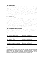
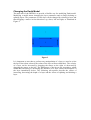
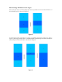
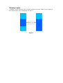
Interactive Receiver Function Forward Modeller-2
(IRFFM2 v1.2)
Hrvoje Tkalčić with contributions from Debdeep Banerjee, Jason Li and Chris Tarlowski Research School of Earth Sciences
The Australian National University
Canberra, Australia
October 2015
All rights reserved.
General Information & User Manual
Research School of Earth Sciences, The Australian National University e-­‐mail: [email protected] | tel. +061 (0)2 6125 3213 www: http://rses.anu.edu.au/~hrvoje/ A note to IRFFM2 users
The predecessor to IRFFM2 was IRFFM. The abbreviation stands for Interactive
Receiver Function Forward Modeller. It is a Java program written during 2008/09 for
interactive forward modelling of receiver functions (RFs) and it is featured for the
first time in Tkalčić et al. (2011) in a study of lithospheric structure of southeast
China. IRFFM2 is an extension of IRFFM – it enables a joint modelling of receiver
functions (RFs) and surface wave dispersion (SWD). It was presented and used in
Tkalčić et al. (2012) in a study on lithospheric structure of southeast Australia.
IRFFM2 is a useful complement to the inversion or a stand-alone tool. An easy-to-use
graphic interface is designed to enable the user to efficiently manipulate lithospheric
thicknesses and velocities, as well as Vp/Vs ratios in a 1D Earth model. It rapidly
displays the theoretical and observed RFs and SWD and provides insights, through
forward modelling, into how a 1D model has to be altered to reduce a misfit between
the observations and theoretical predictions. Input RFs are in a two-column ascii
format, while input SWD are in a three-column ascii format (containing errors in the
third column) and the package comes with an example. The input velocity models are
in ascii format, and the models provided with the package are ak135 (Kennett et al.,
1995) and PREM (Dziewonski et al., 1981). The users can use one of these two as a
starting model, construct their own model from other geophysical constraints, or
simply, guess an initial earth structure. Apart from global velocity models, we
typically start with a resulting model from a grid search, as described in Tkalčić et al.
(2006; 2011), with 3 or 4 layers in the crust and 1 layer in the mantle. It is possible to
save the current model at any time during the forward modelling for the future use, or
upload a new observed RF or SWD at any time.
The method used in IRFFM2 for the calculation of the theoretical RFs consists of the
synthetic seismogram algorithm by G. Randall (respknt), based on the method
developed by Kennett (1983). IRFFM2 v1.1 used a time domain iterative
deconvolution procedure (iterdecon) described by Ligorría and Ammon (1999) to
produce synthetic RFs (in the same manner it is done for the observed RFs).
Therefore, the program was closely tied to the package available from the web site of
Charles J. Ammon (http://eqseis.geosc.psu.edu/~cammon/). However, IRFFM v1.2
featured here uses its own version of iterdecon re-written in Java. Currently available
Gaussian filters are a=1.0, 2.5, 5.0 and 10.0.
Therefore, a remaining part of the IRFFM2 software that is still dependent on
Ammon’s original package is respknt. Another dependent executable is called
dispersion, which computes surface wave dispersion based on the program written by
Saito (1988). The third executable is called sac2asc: it converts sac to ascii files.
N.B. The users should make sure that they have respknt, dispersion and sac2asc
executables compiled and running independently on their Mac before they can
execute IRFFM2. The wrapper script used by IRFFM2 is called IRFFM_SCRIPT, and
all executables are called from that script. Therefore, if executables do not run
properly, IRFFM2 will not work either. All three executables are provided with the
package and should be working on your Mac. If for some reason they do not, their
source codes will be made available upon request.
IRFFM is a work in progress and we welcome and encourage your feedback. The
enquiries and feedback can be sent to [email protected].
REFERENCES
Dziewonski, A.M. & Anderson, D.L., 1981. Preliminary reference Earth model, Phys.
Earth Planet. Inter., 25, 297–356.
Kennett, B.L.N. (1983), Approximations to the response of the stratification, in
Seismic Wave Propagation in Stratified Media, chapter 9, Cambridge Univ. Press,
New York.
Kennett, B.L.N., Engdahl, B.E. & Buland, R., 1995. Constrains on the velocity
structure in the Earth from travel times, Geophys. J. Int., 122, 108–124.
Ligorría, J. P., and C. J. Ammon (1999), Iterative deconvolution and receiver function
estimation, Bull. Seismol. Soc. Am., 89, 1395 – 1400.
Saito,M., 1988. DISPER80: a subroutine package for the calculation of seismic
normal-model solutions, in Seismological Algorithms, pp. 294–319, ed. Doornbos,
D.J., Academic Press, New York.
Tkalčić, H., Pasyanos, M., Rodgers, A., Gök, R., Walter, W. & Al-Amri, A. (2006), A
multi-step approach in joint modeling of surface wave dispersion and teleseismic
receiver functions: Implications for lithospheric structure of the Arabian peninsula,
J. Geophys. Res. 111, B11311, doi:10.1029/2005JB004130.
Tkalčić, H., Y. Chen, R. Liu, Z. Huang, L. Sun and W. Chan, Multi-Step modelling of
teleseismic receiver functions combined with constraints from seismic
tomography: Crustal structure beneath southeast China, Geophys. J. Int., 187, doi:
10.1111/j.1365-246X.2011.05132.x, 303-326, 2011.
Tkalčić, H., N. Rawlinson, P. Arroucau, A. Kumar and B.L.N. Kennett, Multi-Step
modeling of receiver-based seismic and ambient noise data from WOMBAT array:
Crustal structure beneath southeast Australia, Geophys. J. Int., doi: 10.1111/j.1365246X.2012.05442.x, 189, 1681-1700, 2012.
Introduction
This document describes the functionalities of the IRFFM2 user interface. The
IRFFM2 helps constructing one-dimensional model of the earth that reduces the
misfit between the synthetic and observed receiver functions and surface wave
dispersion curves.
Figure 1: Screen Shot of IRFFM2
The user interface, as seen in Figure 1, consists of four main parts:
1.
2.
3.
4.
The model display section (left hand side)
The receiver function display section (upper right section)
The dispersion curves display section (middle section)
The control panel (bottom right section)
The Model Display
The earth model is displayed on the left-hand side of the main window. The model
display consists of two columns; the left one representing the shear wave speed (Vs)
and the right one representing the ratio of compressional and shear wave speeds
(Vp/Vs). The y-axis of each of these columns shows the depth in kilometres. Each
column is divided into layers of varying thicknesses so that the parameters of the
model are layer thickness, Vs speed, and the Vp/Vs ratio. The procedure for changing
these parameters is described in the sections that follow. Only the layers within the
first 220 kilometres are displayed. The default starting model is the ak135 model (the
file called ak135.mod), which can be modified or replaced later.
The IRFFM2 Display
The observed and the synthetic RFs and SWD curves are displayed at the right hand
corner of the main window. The thick grey line represents the observed RF and the
thin yellow line represents the synthetic RF, calculated from the current model
displayed on the left hand side of the screen. The default observed RF is read from a
file called “example_observed.sac.asc''. The default observed SWD curves are in the
following files provided with the distribution of IRFFM2: “data_disp_love_group”,
“data_disp_love_phase”, “data_disp_rayl_group” and “data_disp_rayl_phase”. These
are 3-column ascii files that contain the period (s) in the first column, the velocity
(m/s) in the second column and the error (m/s) in the third column.
The Dispersion Graphs Display
This section displays 4 pairs of graphs: Love Phase and Group, and Rayleigh Phase
and Group, one for observed and one for synthetic. The following table describes the
legends used in the display:
Legend
Data
Red Filled-Up-Triangle
Observed Love Group
Red Continuous Line
Synthetic Love Group
Red Hollow-Up-Triangle
Observed Love Phase
Red Dashed Line
Synthetic Love Phase
Orange Filled-Up-Triangle
Observed Rayl Group
Orange Continuous Line
Synthetic Rayl Group
Organe Hollow-Up-Triangle
Observed Rayl Phase
Orange Dashed Line
Synthetic Rayl Phase
The Control Panel
The control panel provides the buttons and input fields that enable the user to load
different model files and observed RF files, manipulate a model by deleting or
splitting a layer and execute the program that generates the synthetic RF from the
model data. Further description this functionality will be given at the end.
Changing the Earth Model
The main aim of the IRFFM is to provide a flexible way for modifying Earth model.
Modifying a model means changing the layer parameters and or simply deleting or
splitting layers. The parameters of each layer can be changed by selecting a layer and
then dragging a mouse in four directions: up, down, left and right, as illustrated in
Figure 2.
Figure 2
It is important to note that to perform any manipulation of a layer we need to select
the layer first (when selected, the colour of the layer will turn dark blue). The velocity
of a layer can be increased by dragging the mouse to the right, or decreased by
dragging the mouse to the left. The thicknesses of the layers are associative, which
means that increasing or decreasing the thickness of a layer effects the thickness of
the layer immediately below. The following sub-sections describe the effects of
increasing, decreasing the depth of a layer and the effects of splitting and deleting a
layer.
Increasing Thickness of a Layer
To increase the thickness of a layer, first select the layer and then drag the mouse
pointer downwards. The thickness of the selected layer will increase by the amount
proportional to the movement of the mouse. Figure 3 illustrates the process.
Figure 3
If the depth of the selected layer reached the bottom of the layer below, then the
selected layer will subsume the layer below. In other words, the bottom layer will be
deleted, as described in Figure 4.
Figure 4
Decreasing Thickness of a Layer
First select the layer, and then drag the mouse upwards to decrease the thickness of
the selected layer, as shown in Figure 5.
Figure 5
If the bottom of the selected layer (layer 2) reached the bottom of the layer above
(layer 1), the layer below (layer 3) will absorb the selected layer. In other words, the
selected layer will be deleted, as described in Figure 6.
Figure 6
“Splitting” Layers
There are two ways to divide a layer: 1) splitting a layer by half, and 2) dividing a
layer at a desired point.
1. Select a layer and press “Split Layer” button from the control panel. This will
split the current selected layer into two equal depth layers and the upper half
will be selected. This is illustrated in Figure 7.
Figure 7
2. Specify a position in km from where the selected layer will be split in the field
``Splitting Point'', and then press the “Split Layer'” button in the control panel.
The result of this operation is illustrated in Figure 8.
Figure 8
Deleting Layers
To delete a layer, select the layer to delete and then press the ”Delete Layer'' button in
the control panel. This is illustrated in Figure 9.
Figure 9
The Control Panel
The functions that can be performed from the control panel are described below.
Model Management
The current model file name is displayed in red.





To change the starting synthetic model, press the ”Change Starting Model''
button, and select a new model file. The corresponding synthetic receiver
function will be recalculated.
To save the current model, press “Save Current Model'' button.
To change the parameters of a selected layer, input the new thickness, Vs
speed and Vp/Vs ratio into the corresponding input fields and press the
“Apply'' button.
To split the selected layer, put the depth point form where you want to split
the layer and then press “Split Layer'' button.
To delete the selected layer, press the “Delete Layer'' button.
Receiver Function (RF) Management
The current receiver function file name and the slowness in s/km are displayed in red.



To change the observed receiver function, click on the “Change Observed RF''
button and select a new observed receiver function file. After selection, the
display will be updated.
Four different values of the Gaussian parameter can be selected: 1.0, 2.5, 5
and 10. To change the Gaussian parameter, select one of the parameters and
press the “Run'' button in Controls. At the start, 1.0 is default value of the
Gaussian parameter. Match the value of the Gaussian parameter with the value
you used to calculate the observed receiver function.
To change the slowness, press the “Change Slowness'' button and select a
value. Then press the “Run'' button in Controls. At the start, the default value
is 0.065 s/km. Match the value of the slowness with your best estimate for the
slowness of the observed receiver function.
Surface wave dispersion (SWD) Management
This part of the control panel allows users to selectively display the dispersion graphs.
Note that the default observed values are be read from the files: data_disp_X_Y,
where X can be 'love' and 'rayl', and Y can be 'group' and 'phase'. These 4 files must
be placed in the same location as the jar file (IRFFM2.jar). Initially, all 4 pairs of
graphs are displayed as described in the following figure.
To remove a pair of graph from the dispersion graph display, user must uncheck the
boxes against the type of graphs. The following figure describes the situation where
only two graphs are selected for display.
The source file for the observed dispersion graphs can be changed using the “Change
Obs. X Y” buttons, where X is either Love or Rayleigh and Y is either Phase or
Group.
Mouse Movement Control



Horizontal: The effect of mouse dragging is limited to the x-axis. This means
that only the velocity of a layer can be changed by dragging the mouse to the
left or right. This is the default setting.
Vertical: The effect of mouse dragging is limited to the y-axis. This means
that only the thickness of the layers can be changed by dragging the mouse up
or down.
Any: This option does not limit the effects of mouse-dragging, and both the
thicknesses and the velocities of the selected layers can be changed
simultaneously. This is often less convenient than it looks.
Controls






Run: When the ``Run'' button is pressed, a script is called and the output is
written in the file “outmodel.slowness-param.filter-value.eqr.asc''. For
example, if the slowness is 0.065 s/km, and the Gaussian parameter is 1.0,
then the generated file name will be outmodel.0.065.1.0.eqr.asc. This file will
be read and displayed in the display section.
Reset: Resets everything to the starting points with their default values.
Print to File: Prints a 'jpg' image file containing the Model and RF display
Print to Printer: Prints Model and RF display via selected printer. User
should choose Landscape mode of printing to get desired print.
Quit: Quits the application.
About: Information about the IRFFM2 program.