Download User Manual - Home | Nano | University of Pittsburgh

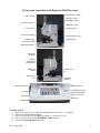
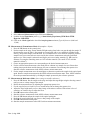
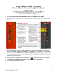
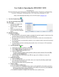
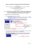
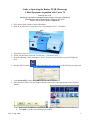
Guide to Operating the Bruker FT-IR Microscope
I. Basic Spectrum Acquisition with Vertex 70
Susheng Tan, Ph.D.
NanoScale Fabrication and Characterization Facility, University of Pittsburgh
M104 Benedum Hall, 3700 O’Hara St., Pittsburgh, PA 15261
Phone: (412) 383-5978, Email: [email protected]
1. Fill in the log-book with the required information.
2. Open the N2 inlet valve to purge the Vertex 70 spectrometer for 15 – 20 minutes
Status
Beam Spliter
Detectors
Specimen
3. Turn on the Vertex 70 spectrometer
4. fill LN2 into the Dewar of the MCT-A detector (~2 full funnels of LN2)
5. check the Humidity, Laser, and Status on Vertex 70 spectrometer and make sure the LED lights are
green
6. Start the OPUS software,
. In the Login dialog box, select your User ID and enter your password
7. on the About OPUS window click OK to open the OPUS interface
8. If the startup test failed, click the diagnosis button or the red dot at the right bottom corner of OPUS
interface
a. Double click the Failed as indicated and Run PQ test for Failed (skip the last Failed one)
b. Click Quit to exit the successful diagnosis window
Rev. 3, Aug. 2009
1
9. Spectrum Acquisition
a. From the menu, select Measure -->Routine Measurement or Advanced Measurement
b. Make necessary changes of the Measurement Parameters
i. On Basic tab: type your Sample description and Sample form
ii. On Advanced tab:
1) Load an appropriate Experiment ( e.g. c:\data\default_Experiment_XPM\
Basic-FT-IR-Transmission-MIR.XPM)
2) Type your File name, and select the correct data Path
3) Set Resolution: 4 cm-1
4) Sample scan time: 16 Scans
5) Background scan time: 16 Scans
6) Save data from 400 cm-1 to 4000 cm-1 (MCT-A detector: 12,000-600 cm-1;
DLATGS: 12,000-350 cm-1; FIR FLATGS: 700-10 cm-1. KBr broadband
splitter: 10,000-400cm-1; Multilayer splitter: 680-30 cm-1)
7) Result spectrum: Transmittance
8) Data blocks to be saved: Transmittance; Single Channel; Background
iii. Optics tab:
1) External synchronization: off
2) Source setting: MIR
3) Beamsplitter: KBr-Broadband
4) Optical Filter setting: Open
5) Aperture setting: 1.5 mm
6) Accessory: Any
7) Measurement channel: Sample Compartment
8) Background meas. Channel: Sample compartment
9) Detector setting: LN-MCT Mid [internal pos. 2]
10) Scanner velocity: 10 Hz
11) Sample signal gain: Automatic
12) Background gain: Automatic
13) Delay after device change: 0
14) Delay before measurement: 0
15) Optical bench ready: OFF
iv. Acquisition tab (usually do not have to be changed):
1) Wanted high frequency limit:
2) Wanted low frequency limit:
3) Laser wavenumber: 15798.30 (unchangeable)
4) High Pass filter: open
5) Low Pass filter: 10kHz
6) Acquisition mode: Double Sided, Forward-Backward
7) Correlation mode: OFF
8) External analog signal: No Analog Value
v. FT tab (usually can leave them unchanged):
1) Phase resolution: 100
2) Phase Correction mode: Mertz
3) Apodization function: Blackman-Harris 3-Term
4) Zerofilling factor: 2
vi. Beam Path tab: make sure the beam path is right for your
measurement
vii. Check Signal tab:
1) check the Interferogram option
2) move the scan range arrow buttons to find the peak
3) make sure the Amplitude is 20,000 – 30,000
4) click Save Peak Position
Rev. 3, Aug. 2009
2
c. Background and Sample Measurement
i. To start the background measurement, select the Basic tab and click on the Background
Single Channel button.
ii. After Background Measurement is done, load your sample into the Vertex 70 sample
chamber
iii. Click Sample Single Channel on the Basic tab
iv. On the basis of this single-channel spectrum and the background spectrum measured, a
resulting transmission spectrum will be calculated and displayed in the spectrum
window.
10. Baseline Correction (optional. The key is the sample preparation!):
icon
a. start either from the Manipulate menu or by clicking on the
b. drag-and-drop the spectrum block from the OPUS browser to the File to Correct field
c. click on the Select Method tab and define a particular baseline correction method (optional)
d. click on the Correct button to start the baseline correction
11. Peak Picking:
a. Open the FT-IR file you want to evaluate and make the optional manipulations
b. From the menu, select Evaluation > Peak Picking, or click the
button.
c. click Interactive Peak Picking button to start peak picking
d. Click on the Store button to save the currently displayed peak position values. Thereupon, a
PEAK data block is added to the spectrum file in the OPUS browser.
12. Save Spectra:
a. The original spectrum is automatically saved in the path which you have defined
b. The spectrum or modified spectrum can be saved as a different file using Save File As
command
c. The file is normally saved in OPUS format. However, the Mode and Data Point Table tabs
allow to save the file in JCAMP-DX format, as a plain X-Y data table, in Pirouette (DAT) or in
GALACTIC format (SPC)
13. Shut Down:
a. Exit the OPUS program
b. Turn off the power of the Vertex 70 spectrometer
c. Sign off the instrument by filling the log book
Rev. 3, Aug. 2009
3
II. Spectrum Acquisition with Hyperion 2000 Microscope
LCD illumination control
Video camera
LCD Color control
LCD ON/OFF switch
Binocular eyepiece
Visible light routing
LCD monitor
Aperture position
Turret with objectives
Kohler aperture control
Sample stage
Focusing knob
Main control panel
Visible light intensity
LN2 Dewar
filling port
Detector
compartment:
MCT detector
Visible light
sources
Spectrometer
port
Visible light intensity
Polarizer port
Alignment
aperture
Reflectance mode
Transmittance mode
IR button
VIS button
Detector temperature:
lights up is warning
Start button
VIS/IR button
I. Getting Started
1. Open the N2 inlet valve to purge the Vertex 70 spectrometer for 15 – 20 minutes
2. Turn on the Vertex 70 spectrometer
3. Fill LN2 into the Dewar of the MCT-A detector (~2 full funnels of LN2)
4. Fill LN2 into the Dewar of the HYPERION 2000 microscope
5. Turn on the Hyperion 2000 microscope
Rev. 3, Aug. 2009
4
6. Turn on the LCD video monitor
7. check the Humidity, Laser, and Status on Vertex 70 spectrometer and make sure the LED lights are
green
8. Start the OPUS software,
. In the Login dialog box, select your User ID and enter your password
9. on the About OPUS window click OK to open the OPUS interface
10. If the startup test failed, click the diagnosis button or the red dot at the right bottom corner of OPUS
interface
a. Click the Failed as indicated and Run PQ test for Failed (skip the last Failed one)
b. After a successful diagnosis, click Quit to exit
II. Checking the Signal Intensity
1. Put the pinhole on the stage. Ensure that the light coming from below passes through the pinhole.
2. Press the VIS button and the reflectance mode button on the control panel.
3. Adjust the stage height using the focusing control until you see a sharp image of the pinhole metal
surface.
4. While looking through the binocular eyepiece or observing the video image on the LCD move the
pinhole on the stage to align the hole with the crosshair.
5. Press the transmittance mode button on the main control panel. The result will be a bright and sharp
image with the light passing through the pinhole.
6. A blurred image can be caused by an incorrect stage height or an improper light intensity. Adjust the
stage height and optimize the light intensity.
Rev. 3, Aug. 2009
5
7. Press the IR button on the main control panel.
8. Select Advanced Measurement in the OPUS menu Measure.
9. Load the desired Experiment profile (e.g. c:\data\default_Experiment_XPM\ Basic-FTIRHyperion- MIR.XPM).
10. Click on the Check signal tab to check the interferogram maximum (Typically between 8,000 and
15,000).
III. Measurement in Transmittance Mode (thin samples < 50μm)
1. Press the VIS button on the control panel.
2. Put the sample on the stage. Ensure that the IR light coming from below can pass through the sample. If
the microtome cut or the fibre is big enough use a metal plate with a very small hole (included in the
delivery) and put the sample across the hole. It is recommend not to cover the hole completely with the
sample but to leave some hole area uncovered for the reference measurement using the predefined
aperture size. If the sample is minuscule and fragile put it on a window material (e.g. KBr) used as
substrate. For samples containing water use CaF2-window material. (The cutoff of CaF2-window
material is 900cm-1.)
3. Choose an appropriate aperture size corresponding to the desired measurement area.
4. For the reference measurement move the metal plate or substrate to a sample-free area. Ensure that
nothing intercepts the beam and the detector does not oversaturate. Do not change the aperture size.
Start the reference measurement in the OPUS software measurement menu.
5. For the sample measurement move the metal plate or substrate to position the sample in the optical path
again. Start the sample measurement in the OPUS software measurement menu. Then, OPUS calculates
the result spectrum automatically by dividing the sample spectrum by the reference spectrum.
IV. Measurement in Reflectance Mode (thin coatings on metallic substrates)
1. Press the VIS button. Put the sample on the stage and adjust the stage height using the focusing control
until you can see a sharp image of the sample.
2. Define the measurement area by adjusting the appropriate aperture size.
3. Use the supplied mirror for the reference measurement. Do not change the aperture size.
4. Adjust the stage height until you see a sharp image of the mirror scratches. If the mirror is free of
scratches, use a mirror edge to adjust the focus.
5. Press IR button on the control panel.
6. Start the reference measurement in the OPUS software measurement menu.
7. Press the VIS button and put the sample in the optical path again.
8. Readjust the stage height until you can see a sharp image of the sample.
9. Press IR button on the control panel.
10. Start the sample measurement in the OPUS software measurement menu.
Rev. 3, Aug. 2009
6