Download The Pennsylvania State University

The Pennsylvania State University
The Graduate School
Department of Mechanical and Nuclear Engineering
GPS/INS SENSING COORDINATION FOR VEHICLE STATE
IDENTIFICATION AND ROAD GRADE POSITIONING
A Thesis in
Mechanical Engineering
by
Ryan David Martini
© 2006 Ryan David Martini
Submitted in Partial Fulfillment
of the Requirements
for the Degree of
Master of Science
August 2006
I grant The Pennsylvania State University the nonexclusive right to use this work for the
University's own purposes and to make single copies of the work available to the public
on a not-for-profit basis if copies are not otherwise available.
Ryan Martini
The thesis of Ryan Martini was reviewed and approved* by the following:
Sean N. Brennan
Assistant Professor, Department of Mechanical and Nuclear Engineering
Thesis Advisor
H.J. Sommer III
Professor and Interim Head Department of Mechanical and Nuclear
Engineering
Thesis Reader
Stefan Thynell
Professor-In-Charge of Graduate Programs in Mechanical and Nuclear
Engineering
*Signatures are on file in the Graduate School
iii
ABSTRACT
This work demonstrates a methodology of estimating vehicle states through the use of a
GPS/INS based sensing architecture.
A sensing system has been developed and
implemented in a vehicle for real-time data acquisition and model based state prediction.
The experimental data is then used to modify existing dynamic models to improve their
accuracy. Modeling results are presented in both the time and frequency domain.
A novel method of longitudinal positioning has also been developed. The method uses
pitch angle measurements to estimate the disturbances input to the system from the road
surface. An estimation of road grade can then be made to increase the accuracy of the
longitudinal positioning solution.
A model inversion process is used to make this
positioning routine possible for any road vehicle. By utilizing a road grade map, the
measurements of commercial grade inertial sensors may achieve positioning accuracy
equivalent to that of a high end differential GPS system.
iv
TABLE OF CONTENTS
LIST OF FIGURES ..................................................................................................... viii
0H
LIST OF TABLES....................................................................................................... xiii
1H
ACKNOWLEDGEMENTS......................................................................................... xiv
2H
Chapter 1 Introduction ................................................................................................ 1
3H
1.1 Motivation....................................................................................................... 1
1.2 Outline of Remaining Chapters ...................................................................... 4
4H
5H
Chapter 2 Introduction to GPS and INS: History, Background and Basic
Functions............................................................................................................... 7
6H
2.1 GPS Background ............................................................................................ 7
2.1.1 Space Segment...................................................................................... 7
2.1.2 Control Segment................................................................................... 8
2.1.3 User Segment........................................................................................ 9
2.2 GPS Functionality........................................................................................... 9
2.2.1 Ideal Description .................................................................................. 10
2.2.2 Technical Description........................................................................... 11
2.2.2.1 Satellite Signals ................................................................................. 11
2.2.2.2 Calculating Position ................................................................... 13
2.2.2.3 Single and Dual Frequency Receivers........................................ 16
2.2.3 Differential GPS ................................................................................... 17
2.2.3.1 DGPS Issues............................................................................... 18
2.3 INS Background ............................................................................................. 18
2.4 INS Functionality............................................................................................ 19
2.5 GPS/INS Integration...................................................................................... 19
7H
8H
9H
10H
11H
12H
13H
14H
15H
16H
17H
18H
19H
20H
21H
Chapter 3 Two Degree-of-Freedom Model ................................................................ 22
22H
3.1 Bicycle Model Derivation............................................................................... 22
3.1.1 Derivation of Understeer Gradient ....................................................... 26
23H
24H
Chapter 4 Vehicle Systems and Integration................................................................ 31
25H
4.1 Vehicle System Layout................................................................................... 31
4.1.1 Part 1: Rover Station – GPS/INS system ............................................. 32
4.1.1.1 GPS/INS Integration .................................................................. 34
4.1.1.2 Rover Station Calibration........................................................... 35
4.1.2 Part 2: Base Station – GPS system ....................................................... 38
26H
27H
28H
29H
30H
v
4.1.2.1 Base Station Calibration............................................................. 39
4.1.3 Part 3: Steering Sensors........................................................................ 40
4.1.3.1 Steering Sensor Calibration........................................................ 41
4.1.4 Data Acquisition System ...................................................................... 43
4.1.4.1 DSP Operation............................................................................ 43
4.1.4.1.1 Interface DSP ................................................................... 44
4.1.4.1.2 Master DSP ...................................................................... 46
4.1.4.2 PC Operation .............................................................................. 47
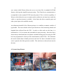
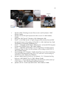
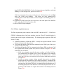
4.2 System Setup Pictures..................................................................................... 48
31H
32H
33H
34H
35H
36H
37H
38H
39H
Chapter 5 Vehicle Parameter and State Estimation – Measurements and Bicycle
Model Predictions................................................................................................. 50
40H
5.1 Vehicle Parameter Estimation ........................................................................ 50
5.1.1 Mass and Vehicle Dimensions..................................................................... 50
5.1.2 Understeer Gradient.............................................................................. 51
5.1.3 Cornering Stiffness Estimation............................................................. 54
5.2 Bicycle Model Simulation Results ................................................................. 57
5.2.1 Chirp Response..................................................................................... 57
5.2.2 Steady-State Circles.............................................................................. 59
5.2.3 Frequency Response............................................................................. 60
5.2.4 Bicycle Model Results Discussion ....................................................... 62
5.3 Bicycle Model – Cornering Stiffness Correction ........................................... 63
5.3.1 Bicycle Model DC Gain Derivations ................................................... 64
5.3.2 Alternate DC Gain Derivation.............................................................. 65
5.3.3 Cornering Stiffness Values from DC Gains ......................................... 67
5.4 Bicycle Model – Cornering Stiffness Correction Simulation Results ............ 70
5.4.1 Chirp Response..................................................................................... 71
5.4.2 Steady-state Circles .............................................................................. 72
5.4.3 Frequency Response............................................................................. 73
5.4.4 Bicycle Model – Cornering Stiffness Correction Results Discussion.. 74
5.4.4.1 Chirp Response .......................................................................... 74
5.4.4.2 Steady-state Circles .................................................................... 75
5.4.4.3 Frequency Response................................................................... 76
5.5 Conclusions..................................................................................................... 76
41H
42H
43H
44H
45H
46H
47H
48H
49H
50H
51H
52H
53H
54H
55H
56H
57H
58H
59H
60H
61H
62H
Chapter 6 Bicycle Model – Tire Lag .......................................................................... 78
63H
6.1 Bicycle Model with Tire Lag Derivation........................................................ 78
6.2 Tire Lag Model – Simulation Results............................................................. 80
6.2.1 Frequency Response............................................................................. 81
6.2.2 Chirp Response..................................................................................... 84
6.2.3 Steady State Circles.............................................................................. 85
6.3 Tire Lag Model – Results Discussion............................................................. 86
64H
65H
66H
67H
68H
69H
vi
6.3.1 Frequency Response............................................................................. 86
6.3.2 Chirp Response..................................................................................... 87
6.3.3 Steady State Circles.............................................................................. 89
6.4 Conclusions..................................................................................................... 90
70H
71H
72H
73H
Chapter 7 Bicycle Model – Camber Correction ......................................................... 92
74H
7.1 Camber Correction Derivation ....................................................................... 92
7.2 Camber Correction – Simulation Results ....................................................... 98
7.2.1 Steady-state Circles .............................................................................. 98
7.3 Conclusions..................................................................................................... 100
75H
76H
77H
78H
Chapter 8 Terrain Disturbances for Longitudinal Positioning.................................... 101
79H
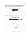
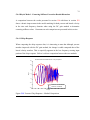
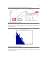
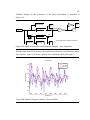
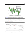
8.1 Initial Terrain Disturbance Observations........................................................ 101
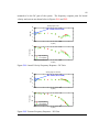
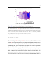
8.2 Road Grade Estimation................................................................................... 102
8.3 Road Grade Repeatability and Location Dependence .................................... 105
8.4 Road Grade Positioning.................................................................................. 107
8.5 Longitudinal Positioning ................................................................................ 113
8.6 Results Discussion .......................................................................................... 116
8.7 Conclusions..................................................................................................... 118
80H
81H
82H
83H
84H
85H
86H
Chapter 9 Pitch Model Derivations and Implementation ........................................... 120
87H
9.1 Free Body Diagram and Assumptions............................................................ 120
9.2 Model 1 – Kinematic Model........................................................................... 122
9.3 Model 2 – Identical Suspensions, No Rotational Inertia ................................ 128
9.4 Additional Suspension Models ....................................................................... 131
9.5 Suspension Parameter Estimation................................................................... 131
9.5.1 Spring Stiffness Estimation .................................................................. 132
9.5.2 Damping Coefficient Estimation .......................................................... 133
9.6 Effect of Forward Velocity on Pitch Measurements and Model Inversion .... 138
9.6.1 Model 1 - Kinematic Model ................................................................. 139
9.6.2 Model 2 - Identical Suspension Model................................................. 142
9.7 Model Inversion on Experimental Data.......................................................... 150
9.8 Conclusions..................................................................................................... 153
88H
89H
90H
91H
92H
93H
94H
95H
96H
97H
98H
99H
Chapter 10 Conclusions .............................................................................................. 155
100H
10.1 System Integration ........................................................................................ 155
10.2 Planar Model State Identification ................................................................. 156
10.3 Road Grade Positioning................................................................................ 157
10.4 Future Work.................................................................................................. 158
10.4.1 System Integration.............................................................................. 158
10.4.2 Planar Model State Identification....................................................... 159
101H
102H
103H
104H
105H
106H
vii
10.4.3 Road Grade Positioning...................................................................... 159
107H
Appendix A Pitch Model Derivation Details.............................................................. 162
108H
A.1 Padé Approximation Discussion.................................................................... 162
A.2 Model 2 – Identical Suspensions, No Rotational Inertia ............................... 164
A.3 Model 3 – Different Suspensions, No Rotational Inertia............................... 165
A.4 Model 4 – Full Pitch Plane Model ................................................................. 169
109H
110H
111H
112H
Appendix B Detailed Interface DSP Operation .......................................................... 174
113H
B.1 Data Retrieval from DL-4plus ....................................................................... 174
B.2 DL-4plus Log Parsing.................................................................................... 176
B.3 Data Read from Steering Sensors .................................................................. 179
114H
115H
116H
Appendix C GPS/INS Setup and Troubleshooting Guide .......................................... 181
117H
C.1 Current Setup Procedure ................................................................................ 181
C.1.1 Base Station Setup ............................................................................... 181
C.49.2 Rover Station Setup ........................................................................... 184
C.49.2.1 GPS/INS System...................................................................... 184
C.49.2.2 Data Acquisition System ......................................................... 186
C.49.2.3 Data Acquisition – Saving Data .............................................. 189
C.2 Troubleshooting ............................................................................................. 190
C.50.1 Reprogramming the Base Station ...................................................... 192
C.50.2 Reprogramming the Rover Station .................................................... 192
C.50.3 Reprogramming the Modems ............................................................ 193
C.50.3.1 Base Station Modem................................................................ 193
C.50.3.2 Rover Station Modem.............................................................. 195
C.50.3.3 Modem Loop Testing .............................................................. 195
C.50.4 Data Acquisition Troubleshooting..................................................... 196
118H
119H
120H
121H
122H
123H
124H
125H
126H
127H
128H
129H
130H
131H
viii
LIST OF FIGURES
Figure 2.1: Replica and Received Signal Comparison ................................................ 10
132H
Figure 2.2: Ideal GPS Positioning ............................................................................... 11
133H
Figure 2.3: Bi-phase Modulation of Carrier Wave ...................................................... 12
134H
Figure 3.1: Bicycle Model ........................................................................................... 22
135H
Figure 3.2: SAE Coordinate System Definition .......................................................... 23
136H
Figure 3.3: Wheel Velocity Vector Summation .......................................................... 25
137H
Figure 3.4: Bicycle Model - Steady State Turn ........................................................... 27
138H
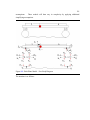
Figure 4.1: System Layout........................................................................................... 32
139H
Figure 4.2: NovAtel DL-4 Plus Receiver .................................................................... 33
140H
Figure 4.3: Honeywell HG1700 IMU – NovAtel Enclosure ....................................... 34
141H
Figure 4.4: Base Station Location................................................................................ 40
142H
Figure 4.5: Steering Sensor Calibration....................................................................... 42
143H
Figure 4.6: DAQ Overview.......................................................................................... 43
144H
Figure 4.7: Interface DSP Algorithm........................................................................... 45
145H
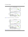
Figure 5.1: Understeer Gradient Calculation – 30.5 m Circle, Clockwise ................. 52
146H
Figure 5.2: Bicycle Model SS Turn – Sideslip View .................................................. 54
147H
Figure 5.3: Sideslip Measurements – Cornering Stiffness Estimation ........................ 56
148H
Figure 5.4: Yawrate Chirp Response – Kus Method ................................................... 58
149H
Figure 5.5: Lateral Velocity Chirp Response – Kus Method....................................... 58
150H
Figure 5.6: Yawrate Steady-State Circle Response – Kus Method ............................ 59
151H
Figure 5.7: Lateral Velocity Steady-State Circle Response – Kus Method................ 60
152H
Figure 5.8: Yawrate Frequency Response – Kus Method ........................................... 61
153H
ix
Figure 5.9: Lateral Velocity Frequency Response – Kus Method............................... 62
154H
Figure 5.10: Sideslip Vector ........................................................................................ 66
155H
Figure 5.11: Lateral Velocity Frequency Response – DC Gain .................................. 68
156H
Figure 5.12: Yawrate Frequency Response – DC Gain............................................... 68
157H
Figure 5.13: Yawrate Chirp Response – DC Gain Method ......................................... 71
158H
Figure 5.14: Lateral Velocity Chirp Response – DC Gain Method............................. 71
159H
Figure 5.15: Yawrate Steady-State Circle Response – DC Gain Method ................... 72
160H
Figure 5.16: Lateral Velocity Steady-State Circle Response – DC Gain Method....... 72
161H
Figure 5.17: Yawrate Frequency Response – DC Gain Method ................................. 73
162H
Figure 5.18: Lateral Velocity Frequency Response – DC Gain Method..................... 73
163H
Figure 5.19: Yawrate Chirp Response – Method Comparison .................................... 74
164H
Figure 5.20: Lateral Velocity Chirp Response – Method Comparison ....................... 75
165H
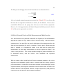
Figure 6.1: Yawrate – Frequency Response Varying Relaxation Length ................... 81
166H
Figure 6.2: Lateral Velocity – Frequency Response Varying Relaxation Length....... 82
167H
Figure 6.3: Yawrate – Frequency Response Best Fit Relaxation Lengths .................. 83
168H
Figure 6.4: Lateral Velocity – Frequency Response Best Fit Relaxation Lengths...... 83
169H
Figure 6.5: Yawrate – Chirp Response Lag Model ..................................................... 84
170H
Figure 6.6: Lateral Velocity – Chirp Response: Lag Model........................................ 84
171H
Figure 6.7: Yawrate – Steady State Circle: Lag Model ............................................... 85
172H
Figure 6.8: Lateral Velocity – Steady State Circle: Lag Model .................................. 85
173H
Figure 6.9: Yawrate – Lag Model and Bicycle Model Comparison – Freq Resp ....... 86
174H
Figure 6.10: Lateral Velocity – Lag Model and Bicycle Model Comparison – Freq
Resp ...................................................................................................................... 87
175H
Figure 6.11: Yawrate – Lag Model and Bicycle Model Comparison – Chirp............. 88
176H
x
Figure 6.12: Lateral Velocity – Lag Model and Bicycle Model Comparison Chirp ..................................................................................................................... 88
177H
Figure 6.13: Yawrate – Lag Model and Bicycle Model Comparison – SS Circle....... 89
178H
Figure 6.14: Lateral Velocity – Lag Model and Bicycle Model Comparison – SS
Circle..................................................................................................................... 90
179H
Figure 7.1: Vehicle Exhibiting Camber ....................................................................... 93
180H
Figure 7.2: Rotation Spring Suspension Model........................................................... 94
181H
Figure 7.3: Yawrate – Camber Model – SS Circle ...................................................... 99
182H
Figure 7.4: Lateral Velocity – Camber Model – SS Circle.......................................... 99
183H
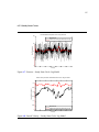
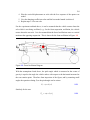
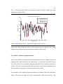
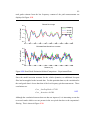
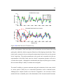
Figure 8.1: Initial Observation of Terrain Disturbance ............................................... 101
184H
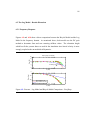
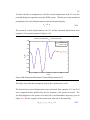
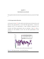
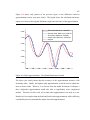
Figure 8.2: Pitch and Road Grade................................................................................ 102
185H
Figure 8.3: Road Grade Estimation – Method Comparison ........................................ 104
186H
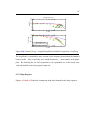
Figure 8.4: Road Grade Repeatability ......................................................................... 106
187H
Figure 8.5: Road Grade................................................................................................ 106
188H
Figure 8.6: View of Error Calculation ......................................................................... 109
189H
Figure 8.7: Road Grade Matches ................................................................................. 111
190H
Figure 8.8: Position Match – Sample 3........................................................................ 112
191H
Figure 8.9: Error Histogram – Sample 3...................................................................... 112
192H
Figure 8.10: Single Lane Experiment .......................................................................... 113
193H
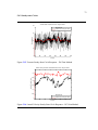
Figure 8.11: Road Grade Velocity Dependence .......................................................... 114
194H
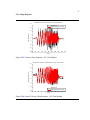
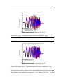
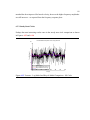
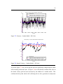
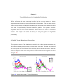
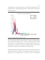
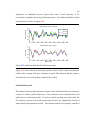
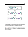
Figure 8.12: Unfiltered Pitch Measurement - FFT ...................................................... 115
195H
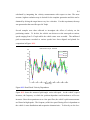
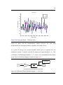
Figure 8.13: Unfiltered and Filtered Pitch Measurements........................................... 116
196H
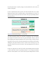
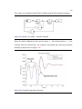
Figure 8.14: Implementation Diagram – Low Pass Filter............................................ 117
197H
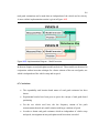
Figure 8.15: Implementation Diagram – Model Inversion .......................................... 118
198H
Figure 9.1: Pitch Plane Model – Free Body Diagram.................................................. 121
199H
xi
Figure 9.2: Kinematic Model – Block Diagram .......................................................... 123
200H
Figure 9.3: Kinematic Model – Frequency Response.................................................. 126
201H
Figure 9.4: Effect of Decreasing Wheelbase ............................................................... 127
202H
Figure 9.5: Identical Suspension Model – Block Diagram.......................................... 128
203H
Figure 9.6: Quarter Car Model – Free Body Diagram................................................. 129
204H
Figure 9.7: Identical Suspension Model – Frequency Response ................................. 130
205H
Figure 9.8: Spring Stiffness Fits .................................................................................. 133
206H
Figure 9.9: Front Oscillation Diagram......................................................................... 134
207H
Figure 9.10: Measured and Estimated Vertical Displacement at CG .......................... 135
208H
Figure 9.11: Quarter Car Model – Simulink Diagram................................................. 136
209H
Figure 9.12: Example Pitch-Plane Excitation.............................................................. 136
210H
Figure 9.13: Quarter Car Model Fits............................................................................ 137
211H
Figure 9.14: Kinematic Model Simulink Diagram - Pitch Generation........................ 139
212H
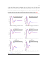
Figure 9.15: Kinematic Model Disturbance Plots........................................................ 140
213H
Figure 9.16: Kinematic Model – Generated Pitch ....................................................... 141
214H
Figure 9.17: Kinematic Model Simulink Diagram – Ur Recovery .............................. 141
215H
Figure 9.18: Kinematic Model – Original Rear Input and Recovered Ur .................... 142
216H
Figure 9.19: Identical Suspension Model Simulink Diagram – Pitch Generation....... 143
217H
Figure 9.20: Identical Suspension Model – Generated Pitch....................................... 143
218H
Figure 9.21: Simulated Pitch Measurements - FFT ..................................................... 144
219H
Figure 9.22: Identical Suspension Model – Low Frequency Pitch............................. 145
220H
Figure 9.23: Pitch Angle and Extracted Rear Road Disturbance................................. 146
221H
Figure 9.24: Identical Suspension Model – Extracted and Actual Rear Disturbance.. 147
222H
Figure 9.25: Road Grade from Road Disturbance Estimations Diagram .................... 147
223H
xii
Figure 9.26: Road Grade from Road Disturbance Estimations Plot............................ 148
224H
Figure 9.27: Model Inversion – Incorrect Model......................................................... 149
225H
Figure 9.28: Aligned Experimental Pitch Measurements ............................................ 150
226H
Figure 9.29: Road Grade Estimation Method Comparison – Experimental Data ....... 151
227H
Figure 9.30: Model Inversion Trend Recovery............................................................ 152
228H
Figure A.1: Padé Approximations – Rear Road Disturbance ...................................... 162
229H
Figure A.2: Padé Approximations – Rear Road Disturbance Zoomed........................ 163
230H
Figure A.3: Different Suspension Model – Frequency Response................................ 166
231H
Figure A.4: Different Suspension Model – Model Check ........................................... 167
232H
Figure A.5: Full Model – Frequency Response ........................................................... 171
233H
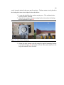
Figure C.1: Base Station Mounting ............................................................................. 182
234H
Figure C.2: Radio Antenna Mounting ......................................................................... 183
235H
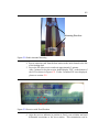
Figure C.3: Receiver with Fixed Position.................................................................... 183
236H
Figure C.4: IMU Mounting.......................................................................................... 184
237H
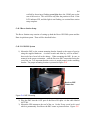
Figure C.5: GPS Antenna Mounting ........................................................................... 185
238H
Figure C.6: DSP-DSP Connections ............................................................................. 187
239H
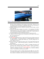
Figure C.7: Steering Sensor Connection ..................................................................... 188
240H
Figure C.8: Connecting to the Client........................................................................... 189
241H
Figure C.9: Saving Active Plots .................................................................................. 190
242H
Figure C.10: Base Station Modem Operation Mode ................................................... 194
243H
Figure C.11: Base Station Modem Baud Rate Settings............................................... 194
244H
xiii
LIST OF TABLES
Table 3.1: Bicycle Model Parameters.......................................................................... 23
245H
Table 4.1: Leverarm Estimate...................................................................................... 37
246H
Table 4.2: Calculated Leverarm................................................................................... 37
247H
Table 4.3: Vehicle Angular Offsets ............................................................................. 38
248H
Table 4.4: Base Station Position .................................................................................. 39
249H
Table 5.1: NHTSA and Measured Vehicle Parameters ............................................... 51
250H
Table 5.2: Understeer Gradient Calculation Results.................................................... 53
251H
Table 5.3: Calculated and Best Fit Ackerman Angles................................................. 53
252H
Table 5.4: Bicycle Model Parameters.......................................................................... 57
253H
Table 5.5: Measured DC Gains.................................................................................... 69
254H
Table 6.1: Best Fit Relaxation Lengths........................................................................ 82
255H
Table 8.1: Average Error Estimates and Correlation Values....................................... 110
256H
Table 9.1: Pitch Model Parameter Definitions ............................................................ 122
257H
Table 9.2: Spring Deflection Measurements ............................................................... 132
258H
Table B.1: Short Binary INS Message Header Structure ............................................ 175
259H
Table B.2: INSSPDSB Message Structure .................................................................. 177
260H
Table C.1: Troubleshooting Table............................................................................... 191
261H
xiv
ACKNOWLEDGEMENTS
I would first like to thank the National Science Foundation, the Department of
Mechanical Engineering and the Pennsylvania Transpiration Institute for providing me
with the funding and facilities to make my graduate education possible.
Thanks to my advisor, Dr. Brennan for his endless support and guidance throughout the
course of this work. He has taught me a tremendous amount about vehicle dynamics and
research in general; in particular the importance of a literature review. Dr. Brennan gave
me the opportunity to work on some very interesting projects which made my graduate
experience quite unique.
Also, big thanks to my lab group members - especially Vishi, Haftay and Bridget. Vishi
spent many hours helping me over the past two years -I believe every all-nighter I have
ever had was with him. His brilliance still amazes me. With Haftay I share the unique
experience of being both an NSF GK-12 fellow and a student in Dr. Brennan’s lab. He is
the only one who truly understands both sides of the story as we have vented many times
together. Bridget has been through the sometimes painful experience of sharing a test
vehicle with me. Our days in Blue Steel are not to be forgotten – I thank her for her help,
her patience and her ability to calm me down when nothing seems to be working.
I would also like to thank all of the great people I have met during my six year stay in
State College. In particular my undergraduate friends who I still keep in touch with. I
could not have asked for a better crew to spend my time with. You are the only ones who
can truly understand and appreciate my college experience.
And to my girlfriend, Kara – where would I be without you? Four perfect years with you
and my love for you grows stronger every day. Years ago I would have doubted a
relationship like this could have ever existed. Thank you for all of your love and support.
xv
And last but not least, I would like to thank my parents. Over the past six years you have
given me more support than I could have ever hoped for. In a time of crisis, you dropped
everything to be by my side. You helped me through the most difficult experience in my
life and I cannot thank you enough. Your love, hard work and dedication have made me
who I am today. I hope that one day I can be as good of a parent to my children as both of
you are to me. I love you both.
Chapter 1
Introduction
This thesis outlines the development, integration and implementation of a real-time data
acquisition system which utilizes the Global Positioning System and inertial sensors for
vehicle state identification. The system is capable of accurately estimating vehicle states
and supplying control efforts in real-time for modeling, control and guidance.
This work then uses the real-time data acquisition system to investigate the planar
dynamics of a passenger vehicle through the Bicycle Model.
Several methods of
estimating front and rear cornering stiffness values are presented and their effects on the
Bicycle Model are shown through model comparisons. The Bicycle Model is then
modified to account for higher-order phenomena such as tire lag and camber thrust to
increase the model’s accuracy. The effects of these changes are investigated in both the
time and frequency domains.
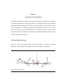
The data collection and modeling efforts of this work revealed very strong terrain
influences on vehicle state measurement. This dependence suggested a new method of
vehicle localization through the analysis of road input disturbances. Pitch-plane vehicle
models were derived and used in an inversion process to assist in this positioning routine
and made the generalization of this positioning methodology possible on any passenger
vehicle.
1.1 Motivation
Over the past several years vehicle research groups in the automotive industry and
academia have turned their focus to integrating computer-based systems into vehicles in
order to increase safety by assisting the driver in high-risk situations. Today, driver-
2
assist systems such the Anti-lock Brake System (ABS) and Electronic Stability Program
(ESP) come standard in many vehicle makes and models. These two systems use various
sensors to detect excessive wheel slip and automatically apply or adjust braking forces
when deemed appropriate. These systems are successful because the control actions can
be applied faster and more consistently by a computer than by the average driver.
As computer processing power increases and cost decreases, more advanced sensing
technology can be integrated into the vehicle. The increased computational power allows
for data processing in real-time and for the development of model-based predictive
algorithms. By continuously monitoring the vehicle states and using this data in vehicle
models running onboard the vehicle, advanced safety systems such as Rollover Detection
and Lane Detection become possible.
In order for these systems to be successful, accurate vehicle models must be developed.
It is critical that the models are sufficiently complex to accurately predict the vehicle’s
dynamics while still remaining as simple as possible to allow real-time implementation
onboard vehicle processors.
A large portion of this work was motivated by a previous study by John Cameron [1]. In
Cameron’s study, a sensing system architecture was developed and used in a vehicle
model comparison between several 3 Degree of Freedom (DOF) roll models found in
literature. The system was used to analyze rollover mitigation algorithms. The sensing
system was based on commercial grade rate sensors and accelerometers which were
inherently noisy and susceptible to drift. Therefore, an accurate estimation of vehicle
attitude (roll, pitch and yaw) was difficult to obtain through integration of these sensor
readings. At the conclusion of Cameron’s work, the quality of the test data was brought
into question as the system exhibited a poor Sensor-to-Noise ratio. It was determined
that a more accurate sensing architecture was needed for a more thorough model
comparison.
3
This thesis began with the development and integration of a military grade GPS/INSbased data acquisition system for vehicle dynamic studies. A detailed description of the
system components, functionality and capabilities is presented. GPS/INS based sensing
has been used extensively in literature with a vehicle dynamics focus [2-9].
Most
relevant to this work are those of Ryu and Bae [4, 9] of Chris Gerdes’ group at the
Dynamic Design Laboratory at Stanford University and the research group of Dave Bevly
[7] of the GPS and Vehicle Dynamics Laboratory at Auburn University. Although the
hardware components used in these other projects are not the same as used here, it must
be noted that these research groups laid important ground work on the subject and
therefore their work will be referenced extensively in this thesis.
With this new sensing system in place, it was necessary to re-perform all experimental
tests presented in Cameron’s work. This includes both frequency- and time-domain
analysis. As a parallel to Cameron’s work, [1], the planar Bicycle Model is revisited.
This work will show significant differences between the results presented in [1] and those
determined with the new sensing architecture. Perhaps the most important model-based
result presented here is a new method of cornering stiffness estimation. Common
methods of cornering stiffness estimation presented in [1] as well as in vehicle dynamics
texts such as [10, 11] were attempted first before a new method is developed. The
differences between the previous methods and the one developed for this work are
explained and discussed.
After the basic low-order planar model is established, higher-order dynamics such as tire
lag and camber effects are investigated and found to be necessary for adequate model fit.
These effects are most easily seen in the frequency domain. Results show that the
addition of these phenomena increases the model’s accuracy without greatly increasing
its complexity.
Throughout the analysis of the experimental data, the effects due to the non-uniform
terrain became apparent. These effects were determined to be highly repeatable and
4
location dependent. These two characteristics allow the terrain effects to be used to assist
in a positioning solution. The terrain influences have been studied previously in works
such as [6] where they were removed from the state estimates to improve state accuracy.
Also, the concept of Road Grade positioning was investigated in [12] where the terrain
effects were identified with commercial grade sensors; however, performance was
limited in positioning accuracy due to its inferior computing and sensing architecture – a
pressure sensor to measure changes in vehicle height – as well as its lack of vehicle
dynamic considerations. This work attempts to eliminate these shortcomings.
This work will also derive and compare multiple Pitch-plane models to help achieve
higher accuracy in a terrain-based positioning method. The goal of incorporating vehicle
dynamics into the correlation algorithm is to allow the terrain disturbance positioning
routine to be used on a wide range of passenger vehicles and speeds.
1.2 Outline of Remaining Chapters
The remaining chapters of this work will structured as follows:
Chapter 2 will present the basic concepts behind GPS and INS systems and their
integration into a vehicle data-acquisition system. Although the fine technicalities of
each of these sensors will not be presented, it is important for the users of the data
acquisition system to have a fundamental understanding of the principles of operation of
each component.
Chapter 3 will present the standard 2 DOF planar Bicycle Model which is used
extensively throughout this work. Its derivation will be given as well as an explanation
of the physics behind the model
5
Chapter 4 will describe the vehicle instrumentation that is used in this study. This
includes the GPS/INS system, the steering sensors and the custom real-time data
acquisition system.
Chapter 5 outlines a methodology of vehicle parameter estimation utilizing data
collection and the Bicycle Model. The experiments performed will be explained, and a
discussion will be given on how the data is post-processed for model comparison. A new
method of cornering stiffness estimation is explained, and it is compared to more
traditional methods that are common in literature.
Chapter 6 will present a modification to the Bicycle Model to incorporate tire lag while
Chpater 7 will add the effects of camber.
Chapter 8 introduces the concept of using Road Grade and road disturbances to help
assist in the positioning solution. The preliminary analysis used as a proof-of-concept is
described before the process is refined further in Chapter 9.
Chapter 9 includes the refinement of the road disturbance positioning routine as well as
the introduction and implementation to several Pitch-plane models. These models are
used in an inversion process to increase the accuracy of the positioning routine and to
generalize measurement of a single vehicle at a single velocity to any vehicle (with
known model) at any velocity. To identify pitch-model characteristics, a method of
estimating vehicle spring constants and damping coefficients is given and the effects of
the model inversion are demonstrated through simulation and experimental data.
Chapter 10 will present the thesis conclusions as well as the future work.
Appendix A consists of the detailed portions of the Pitch-plane model derivations from
Chapter 9.
6
Appendix B outlines a detailed example of the data acquisition code. This is necessary
for users who will follow this work and need to adjust the system to accommodate
additional system inputs.
Appendix C is a data acquisition system troubleshooting guide to be used as necessary.
1.
2.
3.
4.
5.
6.
7.
8.
9.
10.
11.
12.
Cameron, J.T., Vehicle Dynamic Modeling for the Prediction and Prevention of
Vehicle Rollover. 2005: The Pennsylvania State University.
Chen, G. and D.A. Grejner-Brzezinska. Land-Vehicle Navigation Using Multiple
Model Carrier Phase DGPS/INS. in Proceedings of the 2001 American Control
Conference. 2001. Arlington, Virginia.
Farrell, J., T. Givargis, and M. Barth. Differential Carrier Phase GPS-Aided INS
for Automotive Applications. in Proceedings of the 1999 American Control
Conference. 1999. San Diego, California.
Ryu, J., E.J. Rossetter, and J.C. Gerdes. Vehicle Sideslip and Roll Parameter
Estimation using GPS. in AVEC 2002: 6th International Symposium on Advanced
Vehicle Control. 2002. Hiroshima, Japan.
Yang, Y., J. Farrell, and H.-S. Tan. GPS-aided INS based Control State
Calculation for AHS. in Proceedings of the 2001 American Control Conference.
2001. Arlington, Virginia.
Ryu, J. and J.C. Gerdes. Estimation Of Vehicle Roll And Road Bank Angle. 2004.
Boston, Massachusetts.
Bevly, D.M., et al. The Use of GPS Based Velocity Measurements for Improved
Vehicle State Estimation. in Proceedings of the 2000 American Control
Conference. 2000. Chicago, Illinois.
Bevly, D.M., R. Sheridan, and J.C. Gerdes. Integrating INS Sensors with GPS
Velocity Measurements for Continuous Estimation of Vehicle Sideslip and Tire
Cornering Stiffness. in Proceedings of the 2001 American Control Conference.
2001. Arlington, Virginia.
Bae, H.S., J. Ryu, and J.C. Gerdes. Road Grade and Vehicle Parameter
Estimation for Longitudinal Control Using GPS. in Proceeings of IEEE
Conference on Intelligent Transportation Systems. 2001.
Gillespie, T.D., Fundamentals of Vehicle Dynamics. 1992: Society of Automotive
Engineers (SAE). 495.
Karnopp, D., Vehicle Stability. 2004, New York: Marcel Dekker, Inc.
Holzapfel, W., M. Sofsky, and U. Neuschefer-Rube, Road Profile Recognition for
Autonomous Car Navigation and Navstar GPS Support. IEEE Transactions on
Aerospace and Electronic Systems, 2003. 39(1): p. 2-12.
Chapter 2
Introduction to GPS and INS: History, Background and Basic Functions
This chapter will introduce the fundamentals of two major components of the vehicle
sensing system: the Global Positioning System (GPS) and the Inertial Navigation System
(INS). Although it is not necessary to know all theoretical details of these systems in
order to understand the use of GPS in passenger vehicle applications, a conceptual
understanding is necessary for proper implementation and troubleshooting. This chapter
provides an essential foundation for using these sensors in a vehicle dynamic study.
2.1 GPS Background
The Global Positioning System is a Department of Defense operated radio-based
navigation system consisting of 24 satellites orbiting approximately 11,000 miles above
the surface of the earth. The GPS of today has evolved from early radio navigation
systems such as MIT’s LORAN (Long Range Area Navigation) system of the 1940’s [1].
Initially developed for military use, the system was declared available to civilian use in
1983 and by 1984 the commercial GPS market began to take off though its use in
surveying. The Global Positioning System can best be described in three main segments:
Space Segment, Control Segment and User Segment. Below is a description of each,
followed by a description of their integration together.
2.1.1 Space Segment
The space segment consists of a constellation of 24 NAVSTAR (NAVigation Satellite
Timing and Ranging) Satellites which orbit the earth at 11,000 miles above the surface.
The present constellation consists of 24 operational satellites deployed in six evenly
8
spaced planes (A to F) with an inclination of 55 degrees and with four satellites per plane
[2]. This arrangement guarantees 4-8 visible satellites from any given point on the earth
assuming open sky visibility. These solar powered satellites orbit the earth once every 12
hours at a speed of 3.9 km/s. Each satellite is equipped with 4 atomic clocks accurate to a
billionth of a second.
The NAVSTAR’s accuracy is directly affected by the accuracy of each satellite’s
onboard atomic clocks. These clocks are used to synchronize all system processes and to
produce the fundamental L-band carrier frequency on which GPS data is modulated. The
two frequencies used by GPS are denoted L1 (1575.42 MHz) and L2 (1227.60 MHz).
Civilian GPS receivers use only the L1 frequency on which navigation data and Coarse
Acquisition (C/A) code for Standard Positioning Service (SPS) is transmitted. On the
other hand, the L2 frequency only carries P-Code (or encrypted P-Code, called Y code) to
be used by receivers designed for Precision Positioning Service (PPS) – namely military
grade receivers. The C/A code is purposely omitted from the L2 carrier which allows the
Joint Program Office (JPO) to control the information broadcast by the satellites and
allows them to deny full system accuracy to nonmilitary users [2].
2.1.2 Control Segment
The control segment consists of one Master Control Station (MCS) and five Monitoring
Stations (MS). The main operational tasks for the control segment are to track the
satellites for orbit, clock determination and prediction, to perform time synchronization
of the satellites, and to upload this information in a data message to the satellites to
ensure accurate position solutions [2]. One MS is located at the MCS, at the Falcon Air
Force Base in Colorado Springs, Colorado, and the remaining four are located on Hawaii,
Ascension, Diego Garcia and Kwajalein islands. These stations collect altitude, position,
speed and the health of the orbiting satellites for all satellites in view, and send this
information to the MCS for real-time data processing. This whole process is performed
twice a day by each of the Monitoring Stations. From the data collected, the MCS
9
calculates any position or clock errors for each satellite and sends these corrections back
to the satellites for more accurate solutions for the end-user.
2.1.3 User Segment
The user segment is the most well known portion of the entire GPS system. As one may
imagine, this segment is made up of all users who receive GPS satellite data. This
includes military, civilian and commercial users. The uses for GPS amongst these groups
are for the most part, common knowledge. This work will only investigate the use of
GPS in the user segment defined by civilian and commercial users – namely the
automotive industry, and the ability to use a GPS system as a sensor to measure vehicle
states. One must note that upon inception, the Global Positioning System was designed
as a two-tiered system in which military capability was far superior to commercial and
civilian ability. The DoD strictly regulated the accuracy of non-military users though
Selective Availability (SA). Today, the differences between these two sectors have
decreased tremendously as the commercial and civilian sector have researched ways
around SA to improve accuracy without military-grade equipment.
2.2 GPS Functionality
With the three segments outlined, the system can be explained in a straight forward
manner. First, the simple or ideal case can be described to demonstrate how a satellite’s
position in orbit can translate into precise position on the earth’s surface. After the ideal
case is explained, more technical content will be presented.
10
2.2.1 Ideal Description
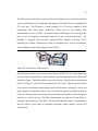
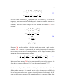
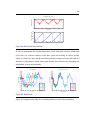
Each satellite transmits its own specific binary code which is modulated on a carrier
frequency. Although the code may appear to be noise, it is actually unique to each
satellite and completely predicable given the right algorithm. Because of this noise-like
appearance, the code is referred to as Pseudo-Random Noise (PRN). Each receiver on
earth has the ability to regenerate the carrier frequencies as well as the PRN codes for
each satellite. When the receiver locks onto a satellite, it can compare the code being
received with that it has stored.
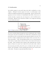
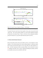
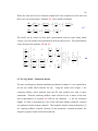
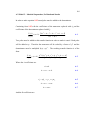
Figure 2.1: Replica and Received Signal Comparison
The receiver can then estimate the signal travel time by subtracting the time its internal
clock registers from the time indicated by the satellite when it transmitted the relevant
pulse (phase lag of the received signal from that generated within the receiver)[1]. The
travel time can then be multiplied by the speed of light to tell the receiver how far it is
from a given satellite – X miles. This then implies that the receiver is located somewhere
on the surface of a sphere that has a radius of X miles, and is centered at the location of
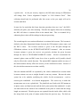
the satellite. When calculated for three satellites in three dimensional space, the three
spheres will intersect at 2 points. One of which will be on the earth’s surface, while the
other intersection point will be either off in space or well below the earth’s surface and
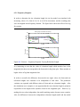
therefore can be disregarded. Thus the remaining point will be the user’s location on the
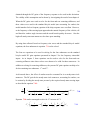
earth’s surface. This process is represented pictorially in Figure 2.2:
262H
11
Figure 2.2: Ideal GPS Positioning
The simple description of GPS operation presented above does not capture all of the
intricacies of GPS. Although many of these issues fall beyond the scope this work, it is
necessary to have a greater understanding than the ‘ideal’ case in order to implement a
GPS system in a vehicle environment. Because of this, a more descriptive, but not a
complete description of the details of GPS has been included below.
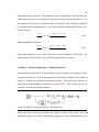
2.2.2 Technical Description
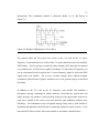
2.2.2.1 Satellite Signals
Each NAVSTAR Satellite transmits three codes in the form of Pseudo-Random Noise
(PRN) modulated on the two carrier frequencies – L1 and L2. There are two ranging
codes referred to as the Coarse Acquisition Code (C/A) and Precision code (P-Code) as
well as a Navigation message code which contains critical satellite information. All three
of these codes are modulated on the L1 frequency, and only the P-code is modulated on
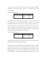
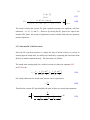
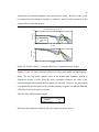
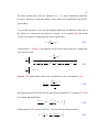
the L2 frequency. They are modulated on each carrier signal by a rarely used modulation
method called Bi-Phase Modulation (as opposed to the Amplitude Modulation (AM) and
Frequency Modulation (FM) of common radio signals). In Phase Modulation the carrier
signals phase reverses when data transmission starts and then re-syncs phase at the end of
12
transmission. This modulation method is discussed further in [2], and shown in
Figure 2.3:
263H
Figure 2.3: Bi-phase Modulation of Carrier Wave
The general public has been given free access to the C/A code on the L1 carrier
frequency. Each satellite has its version of the C/A code characterized by each satellites
PRN number. These messages are relatively short in length (1023 bits) and are repeated
every millisecond. A GPS receiver capable of reading C/A code on the L1 frequency can
use its own internal clock to replicate the L1 carrier frequency signal as well as the PRN
signals from each satellite. The receiver can then compare these replicated signals
(sometimes called reference signals) with those received to generate ranges as described
previously.
In addition to the C/A code on the L1 frequency, each satellite also transmits a
Navigation message containing its orbital elements, clock behavior, system time and
status messages. An almanac is also provided which gives the approximate location for
each active satellite so the receiver can track and lock onto additional satellites more
efficiently. The information in the Navigation message being sent by each satellite is
monitored and updated by the MCS and its monitoring stations to ensure accuracy. At all
times the MCS knows exactly where each satellite is, and where it should be next.
13
Until the year 2000, non-military users operating on the L1 frequency were affected by a
service called Selective Availability (SA). SA is the intentional degradation of GPS
messages on the L1 frequency. SA was put in place by the DoD to stop users from
having dangerously accurate systems.
During this time, when C/A messages were
decoded on a single receiver one could achieve accuracy on the order of 100 meters in the
horizontal direction. As the demand for a more accurate, non-military system increased,
users found ways around SA. This eventually led to the cancellation of SA in 2000 and
users gained access to the full accuracy of the C/A message – approximately 15 meters in
the horizontal direction on a single receiver. This system of receiving and processing
free C/A code on the L1 frequency is known as the Standard Positioning Service (SPS).
The DoD and people authorized by the government can have access to the P-code that is
modulated on both carrier frequencies. When necessary, this code can be further
encrypted to Y-code for added security through a method called anti-spoofing. The code
is much longer than the C/A code at 2e14 bits (37 weeks long). Each satellite transmits a
different 7 day segment of code before the code is reset. The pure length of this message
makes it nearly impossible for unauthorized users to gain access.
Advanced dual
frequency receivers use the C/A code on startup to help track and match the longer Pcode. When demodulated by the receiver, the P-code message gives accuracy to
approximately 5-8 meters. This is known as the Precision Positioning Service (PPS).
2.2.2.2 Calculating Position
Each GPS receiver uses its own internal clock (usually inexpensive quartz crystal
oscillators) to replicate the L-band carrier frequencies as well as the available PRN codes.
It then uses bi-phase modulation to combine the PRN codes with the carrier signal to
generate reference signals for each satellite. By aligning and comparing its reference
signals to those received from the satellites, the receiver can calculate the phase lags
between the two signals. This phase lag corresponds to the signal travel time from the
satellite to the phase center of the GPS antenna. This time multiplied by the speed of
14
light gives the receiver-satellite range. If the receiver’s onboard clock could exactly
match that of the satellite, a receiver would be able to precisely calculate its position from
only three satellite ranges. In practice this is not possible because the quartz clock has an
inherent time drift which creates a timing offset from true GPS time. Because of this
offset, the distance measured to the satellite is slightly longer or shorter than the “true”
range [2]. Thus, the calculated distance is not the true range, but a pseudorange. The
pseudorange measurement can typically be modeled as:
Pn = (t k − t n ) ⋅ c
2.1
Where Pn is the pseudorange between the receiver and satellite n; tk is the receiver clock
time, tn is the satellite transmit time and c is the speed of light.
Both the receiver and satellite have their own clock biases which create errors in the true
range calculation. The satellite clock bias can be modeled as a polynomial whose
coefficients are transmitted to the receiver in the Navigation message [2]. The satellite
bias can then be easily removed from the range calculation. The receiver can then
estimate its own clock bias by calculating pseudoranges for four satellites instead of
three. The four pseudorange equations will allow the receiver to solve for the four
unknowns – three position components and the receiver clock bias. The equation set can
be represented by equation 2.2
264H
( X n − U x ) 2 + (Yn − U y ) 2 + ( Z n − U z ) 2 = ( Pn − C R ) 2 n = 1,2,3,4
2.2
Where Ux, Uy and Uz are the receivers coordinates, Xn,Yn, and Zn are the position
coordinates of satellite n and CR is the receiver clock bias which is common for all four
ranging solutions [1].
The clock bias can then be removed from the pseudorange
calculations for a more accurate position solution.
Rn = Pn − c ⋅ C R
2.3
15
Where Rn is the true distance from satellite n, and Pn is the corresponding pseudorange
and CR is the receiver clock bias. The Code Pseudorange calculation and correction
above can result in approximately 3m accuracy on an L1 single frequency receiver, and
30cm on an L1,L2 dual phase receiver.
Users with very stringent accuracy requirements can utilize Carrier Phase (or Phase
Psedudoranging) GPS. This method of calculating distance measures the phase of the
GPS carrier wave and compares that to the replica carrier [3]. Compared to Code
Pseudorange algorithms, much more accurate position solutions can be achieved: carrierbased algorithms can achieve accuracies of 1-2 cm [4]. This method is typically used in
Real-Time Kinematic differential positioning solutions.
In order to perform this
measurement, the receiver removes the known PRN code from the received satellite
signal. After PRN removal, the received signal still contains the navigation message
which can be decoded and eliminated by high-pass filtering. The final result is the
Doppler-shifted carrier on which phase measurement can be performed [2].
The Carrier Phase to be measured is the difference between phase of receiver’s replica
signal and the signal received plus the number of cycles at the initial start of tracking.
This number will have an integer and fractional component, e.g. 123456789.871 cycles.
The fractional component, if known, can be used to provide additional time resolution
which therefore provides additional resolution in the position estimate.
The derivation of the carrier phase positioning technique is presented in [2] and its details
will not be presented here. The method is based off of electromagnetic wave propagation
and is beyond the scope of this work. The resulting equation however, has been rewritten to agree with previous notation and is presented in equation 2.4
265H
Φ=
1
λ
R+
c
λ
CR + N
2.4
16
Where Φ is the measurable phase, λ is the wavelength, CR is the receiver clock bias, c is
the speed of light, R is the true range and N is the initial number of cycles between the
satellite carrier wave and that replicated by the receiver upon initial signal tracking.
By multiplying the frequency equation, equation 2.4 (expressed in cycles) by the
266H
wavelength, λ, of the carrier a range equation is formed.
Pn = Rn + c ⋅ C R + Nλ
2.5
Rearranging equation 2.5 allows for direct comparison to the Code Pseudorange equation
267H
presented earlier.
Rn = Pn − c ⋅ C R − Nλ
2.6
Comparing equation 2.6 to equation 2.3 shows that the Carrier Phase measurement
268H
269H
differs from the Code Pseudorange measurement by only an integer number of
wavelengths. Hofmann-Wellenhof, [2], points out that the phase of a carrier can be
measured to 1% (0.01 cycles) of its wavelength which corresponds to millimeter
precision, assuming no other errors are introduced.
2.2.2.3 Single and Dual Frequency Receivers
The military-grade dual frequency receivers have several advantages over the single
frequency receivers. Their access to the coded messages on the L1 and L2 frequencies
give them superior accuracy for various reasons, two of which are presented here.
As discussed above, a receiver can calculate its position using Code Pseudoranging or
both Code Pseudoranging and Carrier Phase positioning. If only C/A code is available
for a given receiver, it may only use the above techniques on the messages transmitted on
the L1 frequency. However, if a receiver has access to both C/A and P(Y)-Code, it may
perform these calculations on both frequencies. By having access to the P(Y)-Code on
the L2 frequency, a receiver can directly remove the code from the L2 frequency and use
17
the underlying Doppler shifted carrier frequency for Carrier Phase positioning. Without
knowledge of the P(Y)-code, one has to use codeless or quasi-codeless techniques for
reconstruction of the unmodulated carrier wave from which the phase of the base carrier
is measured [1]. The codeless and quasi-codeless techniques are inherently less accurate
than the coded method.
Another advantage of dual frequency receivers are their ability to estimate ionospheric
and atmospheric delays. In the previous cases, it was assumed that the satellite signal
propagated at the speed of light. It must be noted that this is only true in a vacuum. In
practice, satellite signals see a delay while traveling though the ionosphere which is
approximately proportional to the amount of free electrons the signal encounters [1]. In
the dual frequency system, differences in the Ll and L2 observations are used directly
solve for the ionospheric delay thus reducing ionospheric effects [5].
2.2.3 Differential GPS
Differential GPS (DGPS) was initially developed to eliminate the errors introduced
through SA. It is a system which combines two GPS receivers to produce a position
solution accurate to 3-5 meters even when only standard L1 C/A code is used. One
receiver, referred to as the base station, is setup at a fixed, known location and remains
stationary at that point for its entire operation. This receiver’s job is to receive data from
the L-phase carriers, compute the position indicated by the received data as in ordinary
GPS operation, and then calculate the error between the computed solution and the
known location. The base station estimates the slowly varying error components of each
satellite range measurement and forms a correction for each GPS satellite in view [3].
These error and bias calculations are then broadcasted on a communication link to the
second GPS receiver known as the rover station[4]. The rover is free to move and
receives these corrections via radio, internet or other communication means. The rover
uses the base stations corrections for every satellite used in its position calculations.
18
DGPS operation drastically increases accuracy and almost entirely removes timing biases
due to satellite clock error, ionospheric and tropospheric, and ephemeris prediction errors.
2.2.3.1 DGPS Issues
When considering the use of DGPS as a sensor for vehicle state identification, there are
several issues which need to be resolved. Perhaps the most important issue is the
possibility of GPS outages when a direct line of sight to satellites is not available. A GPS
receiver is not capable of accurate positioning when less than 4 satellites are available for
its calculations. Tunnels, buildings, trees and other environmental factors make GPS
outages common in vehicle applications.
This lack of signal requires the use of
additional sensors to compliment the DGPS system.
Another issue with GPS is the relatively slow update rate of the sensor, only 5 to 20Hz at
best. The low update rate of GPS leads the system to high frequency errors which also
cause problems in vehicle applications.
Because of these shortcomings, alternate sensing configurations have been investigated
for many years. Due to their complimentary nature, much attention has been paid to the
integration of an Inertial Navigation System (INS) to existing GPS systems.
2.3 INS Background
Chatfield, [6], defines Inertial Navigation as the computation of current velocity and
position from initial velocity and position and the time history of the kinematic
acceleration. This definition is based on the concept that a vehicles current velocity is
equal to the initial velocity plus the integral of the vehicles acceleration with respect to
time. Similarly, the vehicles position is equal to its initial position plus the integral of the
vehicles velocity with respect to time.
Therefore if an initial velocity and position is
19
known, it is possible to position a vehicle by simply measuring accelerations and
performing the integration and addition described above.
Inertial Navigation Systems, which perform this type of positioning, were initially
developed in the late 1940’s for aircraft navigation. The systems have since been refined
for high accuracy and small size.
2.4 INS Functionality
INS systems use measurements captured from an Inertial Measurement Unit (IMU) to
calculate position of a vehicle in the inertial frame. The IMU is a sensor which uses three
accelerometers (X, Y, Z) and three rate gyros (roll, pitch and yaw) to measure how a
vehicle is moving and rotating in space.
The system uses these measurements to
integrate and solve differential equations to estimate vehicles position, velocity and
attitude relative to initially known states. These estimates can be made available as fast
as they system computer can calculate them.
Although the INS system can offer high speed, continuous estimates of position, velocity
and attitude, these estimates are subject to integration error over long periods of time.
Small errors in acceleration readings grow as they are integrated over time – this results
in large errors in velocity estimates and even larger errors in position calculations. These
errors make it necessary to restart or correct stand alone INS systems to ensure accurate
operation. Since INS calculates change in system orientation and acceleration, it needs
initial values for these parameters to be input from an external source.
2.5 GPS/INS Integration
The complimentary nature of GPS and inertial navigation has been well known since the
inception of GPS.
In theory, the continuity of the inertial system can both fill in
20
positioning gaps left by GPS satellite outages and reduce the effect of high frequency
GPS errors, while the unbiased nature of the GPS signals can limit the size of the low
frequency errors in the inertial system [7]. The integration of GPS/INS creates an
accurate, high speed positioning system that can continue to operate when satellite
visibility is limited. This integration of these sensors is system-specific but is usually
performed though a Kalman filtering process which corrects the INS positioning solution
with that of the GPS. This integration will be discussed in more detail in Chapter 4.
1.
2.
3.
4.
5.
6.
7.
Logsdon, T., Understanding the NAVSTAR: GPS, GIS and IVHS. Second ed.
1995, NY, NY: Van Nostrand Reinhold.
Hofmann-Wellenhof, B., H. Lichtenegger, and J. Collins, GPS: Theory and
Practice. Fourth, revised edition ed. 1997, Austria: Springer-Verlag Wien New
York.
Parkinson, B.W. and J.S.J. (eds), Global Positioning System: Theory and
Applications, Volume II. In: Progress in Astronautics and Aeronautics, Vol 164,
ed. P. Zarachan. 1996, Washington, D.C.: American Institute of Aeronautics and
Astronautics, Inc.
Novatel, OEM4 Family of Receivers User Manual - Vol. 1 Installation and
Operation, OM-20000046, Rev. 19. 2005: Alberta, Canada.
Janet Brown-Neumann, A.M., Thomas Ford, Orest Mulyk, Test Results from a
New 2 cm Real Time Kinematic GPS Positioning System. 1996: The Institute of
Navigation, Washington DC. p. 183.
Chatfield, A.B., Fundamentals of High Accuracy Inertital Navigation. Progress in
Astronautics and Aeronautics, Vol 174, ed. P. Zarchan. 1997, Washington, D.C.:
American Institute of Aeronautics and Astronautics, Inc.
Tom Ford, J.N., P. Fenton, M. Bobye, J. Hamilton. OEM4 Inertial: A Tightly
Integrated Decentralised Inertial/GPS Navigation System. 2001. Salt Lake City,
Utah.
Chapter 3
Two Degree-of-Freedom Model
The planar dynamics of a vehicle is often represented in the form of single track, 2 degree
of freedom model known as the Bicycle Model. This model has been used extensively
throughout literature because of its ability to accurately model a vehicle’s lateral velocity
and yaw dynamics. It is defined on a body fixed coordinate system which is centered at
the vehicle center of gravity and which rotates and translates with the vehicle. In this
chapter the derivation of the bicycle model and an important handling characteristic, the
understeer gradient, will be given.
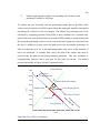
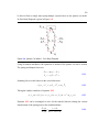
3.1 Bicycle Model Derivation
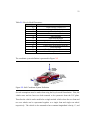
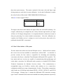
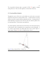
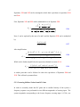
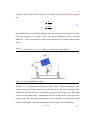
Figure 3.1 shows the Bicycle Model layout and Table 3.1 describes the model
270H
271H
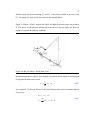
parameters. Note that the tire slip angles are shown to be negative in the figure.
Figure 3.1: Bicycle Model
23
Table 3.1: Bicycle Model Parameters
Symbol
Parameter Description
Vcg,t
U
V
r
β
δf
αf
Vf,t
Ff
αr
Vr,t
Fr
Total velocity vector at CG
Longitudinal velocity
Lateral velocity
Yaw rate about Z axis
Side slip angle
Front steering angle
Front slip angle
Total velocity vector at front tire
Lateral force generated at front tire
Rear slip angle
Total velocity vector at rear tire
Lateral force generated at rear tire
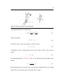
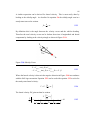
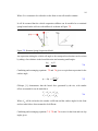
The coordinate system definition is presented in Figure 3.2
272H
Figure 3.2: SAE Coordinate System Definition
Several assumptions must be made when using the bicycle model formulation. First, the
vehicle mass and tire forces are both assumed to be symmetric about the X-Z plane.
Therefore the vehicle can be modeled as a single-tracked vehicle where the two front and
two rear wheels can be represented together as a single front and single rear wheel
respectively. The vehicle is also assumed to have constant longitudinal velocity, U, and
24
tires which roll without slipping in the longitudinal direction. This means there are no
acceleration or braking forces being applied. The front and rear tires are also assumed to
produce lateral forces which are linearly proportional to their respective cornering
stiffnesses. Finally, the model also assumes all angles are small, and therefore the
following simplifications can be applied:
cos(θ ) ≅ 1
sin(θ ) ≅ θ
The states, or variables required to fully describe the motion of the bicycle model are V,
the vehicles lateral velocity at the CG, and r, the angular velocity about the z-axis.
The equation of motion of the vehicle can be derived using Newtonian mechanics as
described below.
Summing forces in the lateral direction, summing moments about the Z axis and applying
the small angle approximation the following equations are obtained:
m ⋅ a y = ∑ Fy = F f cos(δ ) + Fr ≅ F f + Fr
I zz ⋅
dr
= ∑ M z = F f cos(δ ) ⋅ a − Fr ⋅ b ≅ F f ⋅ a − Fr ⋅ b
dt
3.1
Under the assumption that the front and rear tire lateral forces are linearly dependent on
their respective slip angles and cornering stiffnesses, and negative cornering stiffness
values are used
F f = C αf ⋅ α f
Fr = C α r ⋅ α r
3.2
The front and rear slip angles can be solved for by looking at the lateral and longitudinal
velocities at each tire as in Figure 3.3:
273H
25
Figure 3.3: Wheel Velocity Vector Summation
Assuming small angles, we can then write:
⎛ V f ,y ⎞ ⎛ V f ,y
⎟≅⎜
⎟ ⎜V
V
,
f
x
⎝
⎠ ⎝ f ,x
ξ = tan −1 ⎜⎜
⎞
⎟
⎟
⎠
3.3
And from geometry:
α f = ξ −δ f
3.4
The lateral velocity vector for the front tire can be written as:
V f ,y = V + a ⋅ r
3.5
Longitudinal velocity is approximately equal to the vehicles velocity at the center of
gravity:
V f ,x ≅ U
3.6
By combining equations. 3.5, 3.5 , 3.5, and 3.6 the equation for front slip angle can be
274H
275H
276H
277H
formed:
αf =
V + a⋅r
−δ f
U
3.7
By repeating the above procedure for the rear tire and recalling that there is no steering
input at the rear, the equation for rear slip angle can be written
26
αr =
V −b⋅r
U
3.8
Combining equations 3.2, 3.2, 3.7 and 3.8:
278H
279H
280H
281H
⎛V − b ⋅ r ⎞
⎞
⎛V + a ⋅ r
− δ f ⎟ + Cα r ⎜
m ⋅ a y = C αf ⎜
⎟
⎝ U ⎠
⎠
⎝ U
dr
⎛V + a ⋅ r
⎞
⎛V − b ⋅ r ⎞
I zz ⋅
= C αf ⎜
− δ f ⎟ ⋅ a − C αr ⎜
⎟⋅b
dt
⎝ U
⎠
⎝ U
⎠
3.9
3.10
Lateral acceleration in body-fixed coordinates can be expressed as:
ay =
dV
+U ⋅r
dt
3.11
Rearranging equations 3.9 , 3.11 expressions for lateral acceleration and the time rate of
282H
283H
change of the yaw rate can be written:
dV ⎛ Cαf + Cαr
=⎜
dt ⎜⎝ m ⋅ U
⎛ C a − C αr b
⎞
⎞
⎛ − Cαf ⎞
⎟⎟ ⋅ V + ⎜⎜ αf
⎟⎟ ⋅ δ f
− U ⎟⎟ ⋅ r + ⎜⎜
m ⋅U
⎝
⎠
⎠
⎝ m ⎠
⎛ C a 2 + C αr b 2 ⎞
⎛ − C αf a ⎞
dr ⎛ Cαf a − C αr b ⎞
⎟⋅r +⎜
⎟⎟ ⋅ V + ⎜ αf
= ⎜⎜
⎜ m ⎟⎟ ⋅ δ f
⎟
⎜
⋅
dt ⎝ I zz ⋅ U
I
U
zz
⎝
⎠
⎠
⎠
⎝
3.12
3.13
Equations. 3.12 and 3.13 can be represented in standard state space form as in
284H
285H
equation 3.14:
286H
⎡ dV
⎢ dt
⎢ dr
⎢
⎣ dt
⎤ ⎡ C αf + C αr
⎥ ⎢
m ⋅U
⎥ = ⎢C a − C b
αr
⎥ ⎢ αf
⎦ ⎢⎣ I zz ⋅ U
C αf a − C αr b
⎤
⎡ − C αf ⎤
−U ⎥
⎢
⎥
V
⎤
⎡
m ⋅U
m ⎥ ⋅δ
2
2 ⎥⋅⎢ ⎥ + ⎢
f
C αf a + C αr b ⎥ ⎣ r ⎦
⎢ − C αf a ⎥
⎥
⎢⎣ m ⎥⎦
I zz ⋅ U
⎦
3.14
3.1.1 Derivation of Understeer Gradient
A vehicle’s handling behavior can be characterized by a parameter known as the
understeer gradient. In this study, the understeer gradient will be used for its ability to
relate a vehicles weight distribution to its tires’ force generating abilities. The understeer
gradient is a widely used parameter in vehicle dynamics, and its full derivation can be
27
found in many text books including [1], and [2]. It was also presented in previous work,
[3]. For simplicity, only a brief derivation has been included here.
Figure 3.4 shows a 2 DOF, single track vehicle in a high speed steady state turn of radius
287H
R. The forces are shown in the positive direction; however the slip angles are shown as
negative in agreement with SAE standards.
Figure 3.4: Bicycle Model - Steady State Turn
By summing the interior angles of the triangle, an equation for the required steering input
to negotiate the turn can be solved:
δf =
L
−α f +αr
R
3.15
As in equation 3.1 the sum of forces in the lateral direction the sum of moments about he
288H
Z axis gives:
m ⋅ a y = F f + Fr
I zz ⋅
dr
= F f ⋅ a − Fr ⋅ b
dt
3.16
28
In a steady state turn the acceleration in the lateral direction is exactly equal to the
centripetal acceleration:
U2
ay =
R
3.17
In order for the vehicle to be at steady state, it must be in equilibrium about its center of
gravity, and therefore the sum of moments about the z axis must be zero. By combining
equations 3.16, 3.17 and setting the sum of moments to zero gives:
289H
290H
U2
= F f + Fr
R
F f ⋅ a = Fr ⋅ b
m
3.18
3.19
In the standard bicycle model derivation, the lateral force generated by the tires was
assumed to be proportional to each tires’ cornering stiffness. Therefore equations 3.18
291H
and 3.19 can be rearranged and combined with equation 3.2:
292H
293H
b⋅m U 2
⋅
= C αf α f
Ff =
L
R
a⋅m U 2
a
⋅
= Cα r α r
Fr = ⋅ F f =
L
R
b
3.20
Where the cornering stiffness vales are negative quantities. To simplify, recognize that
the weight on the front and rear axle can be written:
m⋅ g
⋅b
L
m⋅ g
Wr =
⋅a
L
Wf =
3.21
Equation 3.20 can then be re-written in terms of vehicle axle weights and solved for the
294H
front and rear slip angles:
αf =
Wf U 2
⋅
Cαf gR
Wr U 2
αr =
⋅
Cαr gR
3.22
29
Combining 3.22 with 3.15 gives:
295H
296H
δf =
L U 2 ⎛⎜ Wr W f ⎞⎟
+
⋅
−
R gR ⎜⎝ Cαr Cαf ⎟⎠
3.23
Again the cornering stiffness values are negative quantities.
Equation 3.23 is used extensively in literature for its ability to correlate parameters
297H
which are easy to measure (steer angle, velocity, turn radius, vehicle length and axle
weights) to quantities which are difficult to measure (front and rear cornering stiffnesses).
From equation 3.23 the understeer gradient, Kus, is defined.
298H
⎛W
Wf ⎞
⎟
K us = ⎜ r −
⎜C
⎟
C
αf ⎠
⎝ αr
3.24
Once again it must be noted that the cornering stiffness values used in equation 3.24 are
299H
negative values.
The understeer gradient derived in this section is important in characterizing the steering
characteristics of a vehicle. A vehicle with a positive understeer gradient will be referred
to as an understeer vehicle. The steering input required for an understeer vehicle to
negotiate a steady state turn increases as the speed of the vehicle increases. On the other
hand, a vehicle with a negative understeer gradient is known as an oversteer vehicle. An
oversteer vehicle actually requires decreasing steering inputs to negotiate a turn for
increasing speeds. Production vehicles are predominately understeer since oversteer
vehicles become unstable in certain turning maneuvers. Further discussion of this topic
can be found in many vehicle dynamics text books, [1, 2], or in previous work [3], and
will not be presented here.
30
1.
2.
3.
Gillespie, T.D., Fundamentals of Vehicle Dynamics. 1992: Society of Automotive
Engineers (SAE). 495.
Karnopp, D., Vehicle Stability. 2004, New York: Marcel Dekker, Inc.
Cameron, J.T., Vehicle Dynamic Modeling for the Prediction and Prevention of
Vehicle Rollover. 2005: The Pennsylvania State University.
Chapter 4
Vehicle Systems and Integration
This chapter will outline the sensing system layout and then present each component of
the system. Pictures of the system are presented at the end of the chapter. A 1992 five
door Mercury Tracer has been selected as the test vehicle for this study. The vehicle is
equipped with a military grade GPS/INS system, linear string potentiometer steering
sensors and an onboard DSP based data acquisition system. The integrated system
currently measures roll, pitch, yaw, velocity magnitude, velocity direction, latitude,
longitude, altitude and steering angle in real time at a rate of 50Hz. If necessary the
system can also output accelerations, angular rates and various other measurements at
100Hz. This system has significant advantages over systems used in previous studies.
4.1 Vehicle System Layout
The current vehicle system can most easily be described in four parts: the Rover Station,
the Base Station, the Steering Sensors and the Data Acquisition system. The Rover
Station, steering sensors and Data Acquisition system are installed in the vehicle while
the Base Station remains outside the vehicle in a fixed location. Each of these parts will
be descried in the subsequent sections of this chapter. Figure 4.1 below shows a general
300H
block diagram of the entire setup:
32
Figure 4.1: System Layout
4.1.1 Part 1: Rover Station – GPS/INS system
The Rover GPS/INS sensing system being used is the NovAtel SPAN (Synchronized
Position Attitude Navigation) system based off two OEM4 dual frequency GPS receivers
and the Honeywell HG1700 military tactical-grade IMU. This GPS/INS combination can
provide estimates of position, velocity and attitude at rates up to 100Hz. In differential
carrier phase fixed-integer mode and with continuous presence of GPS data, the system
achieves a position solution with an accuracy of 2 cm (one sigma). Attitude can be
estimated with an accuracy of 0.013 degrees for roll and pitch and 0.04 degrees for yaw
while velocity error is a mere 0.007 m/s (one sigma) [1].
33
The GPS portion of the Rover system is a NovAtel DL4plus receiver which has modified
software and hardware to accommodate interfacing with the HG1700 over a standard RS232 serial port. The DL4plus is a dual frequency (L1/L2) receiver capable of both
pseudorange and carrier phase positioning. These receivers can transmit GPS
measurements at a rate of 20 Hz. In situations where GPS outages occur, they typically
have L1 and L2 frequency reacquisition times of 0.5 and 1 second respectively. The
DL4plus is equipped with NovAtel’s patented Pulse Aperture Correlator (PAC)
technology to virtually eliminate the effects of multipath errors seen in environments
where buildings or other signal obstacles may exist [2].
Figure 4.2: NovAtel DL-4 Plus Receiver
The INS portion of the system consists of the Honeywell HG1700 AG17 strap-down ring
laser gyro IMU used primarily in missile guidance systems, unmanned aerial vehicles and
standoff weapons. This IMU exhibits a gyro bias of only 10 deg/hr and an acceleration
bias of 3 milli-g [3]. The HG1700 is mounted in a 160 x 160 x 100mm case from which
it can measure accelerations and rotational rates in all directions. Internally, velocity and
angle changes are sampled at 600 Hz. NovAtel’s firmware applies non-linear corrections
to the raw measurements which makes these measurements available in their navigation
software at a 100 Hz rate [4]. The IMU measurements are taken in its body frame as
defined by the sensor axis of the IMU. The measurements then require a transformation
into the vehicle’s body frame to accurately determine vehicle attitude, velocity and
accelerations.
34
Figure 4.3: Honeywell HG1700 IMU – NovAtel Enclosure
4.1.1.1 GPS/INS Integration
The SPAN system integrates the GPS and INS systems through two separate, but
interacting filters in a decentralized Kalman filtering process. A Kalman filter is a
procedure that broadly consists of two steps used to optimally estimate a series of
parameters that describe the behavior of a system [5]. In Real-Time operation, the SPAN
systems decentralized Kalman filter has 15 states: Earth Centered Earth Fixed (ECEF)
position, velocity, attitude Euler angles with respect to the ECEF frame and gyro and
accelerometer biases with respect to the IMU body frame [4]. The filter system collects
IMU’s measurements and time-tags them with the GPS time. It then uses a decentralized
approach to generate a blended GPS/INS solution.
The filtering process of the SPAN system has been referred to as decentralized because
the GPS and inertial processing occur in two separate filters.
The advantages and
disadvantages of using such a process have been discussed in great detail in [4, 5] and
will not be discussed here. The two filters interact by sharing position and position
covariance information. The GPS filter assists the inertial filter by supplying it with GPS
position measurements to be used to control the error growth in the inertial filter. The
inertial filter assists the GPS filter by supplying it with inertial position measurements to
expedite satellite reacquisition times incase of signal interference or blockage.
This
integration process allows the system to be much more accurate than either GPS or INS
35
alone. Further details of the Kalman filtering process, including the exact methodology
of the propagation and update steps of the filter can be found in [5].
4.1.1.2 Rover Station Calibration
The Rover Station’s GPS/INS system required several calibration steps in order to
achieve centimeter level accuracy. The calibration procedure consists of three main steps
which are described below.
The first step of calibration is performed automatically by the DL-4plus and IMU on
startup. When it is initially powered, the IMU has no information regarding its mounting
orientation. Although the IMU is labeled with its own body coordinates, X,Y,Z, it does
not assume that Z is always inline with the gravity vector. In order to resolve its
orientation, a calibration known as frame detection takes place on system startup.
The alignment of the inertial system to the vehicle’s body frame is derived
with a combination of the measured accelerations of the IMU compared to
the gravity vector, and the angular rate measured by the IMU compared to
the earth rate. The alignment computation requires that the system does
not experience any specific forces except gravity, is not physically rotating
except from earth rotation, and that gyro bias in the unit is small compared
to the earth rate [6].
The DL-4plus automatically completes this inertial system alignment after it locks onto
four satellites and an initial position can be calculated from GPS. During this stationary
calibration, the IMU’s roll and pitch alignment is 0.18 degrees while it is only 45 degrees
for yaw. The yaw is particularly inaccurate because of the system is using the latitude
and the earths rotational rate to resolve the yaw angle. This calculation is therefore
skewed by the high gyro drift to earth rate ratio [5]. However, over time the stationary
system will resolve the yaw heading to within a few degrees (approximately 5 degree
accuracy after 300 seconds at 40 degree latitude). In order to expedite the process, the
system should be put in motion after the frame detection and coarse alignment and is
complete. This will make the yaw angle observable and therefore increase its accuracy at
36
a quicker rate.
As the yaw accuracy improves, the INS status message in GPSolution
will change from “Coarse Alignment Complete” to “INS Solution Good.”
Data
collection should only be performed after this occurs as the yaw angle will not be
accurate until then.
It must also be noted that this frame detection procedure does not “zero” the IMU’s
attitudes (roll, pitch, yaw) after mounting. Therefore the angular offsets due to mounting
the IMU will show as constant offsets in the attitude data. This is accounted for by
subtracting these values off the readings in data post processing.
The second stage the rover station calibration is to estimate the leverarm. The leverarm is
defined as the three dimensional distance between the GPS antenna’s phase center, and
the IMU’s center.
The leverarm estimate is given to the DL-4plus through the
GPSolution software via the SETIMUTOANTOFFSET command. After an accurate
leverarm estimate is given, the receiver can precisely calculate the given leverarm
through the built in LEVERARMCALIBRATE routine.
NovAtel recommends the
antenna’s phase center and IMU center be as close as possible, and if possible, should
only be offset in the vertical direction. The antenna/IMU alignment and the accuracy of
the initial estimate directly affect the accuracy of the calculated leverarm. Because of
this, the initial measurement was taken carefully.
Since the antenna and IMU are separated by the vehicle windshield, an accurate initial
leverarm estimate was not as straight forward as one may assume. Because the entire
system has to be modular, modifying the vehicle for this measurement – such as
removing the windshield - was deemed inappropriate. The easiest way to make this
measurement was to use a plumb bob. The plumb bob was fixed to the GPS antenna at
its phase center, and then lowered until the bob’s point touched the windshield. A mark
was then made on the outside of the windshield at the point of contact and the strings
length was measured. Then the process was repeated from the inside of the vehicle with
the string fixed at the point of contact marked from the previous step. The bob was
37
lowered to the center of the IMU, and once again the string length was measured.
Although this is not an exact distance calculation, it was appropriate for an initial
leverarm estimate.
Table 4.1: Leverarm Estimate
Inertial Frame Coordinate
Offset (m)
Uncertainty (m)
X
-0.02
-0.09
0.99
+/- 0.03
Y
Z
+/- 0.03
+/- 0.03
After the initial leverarm estimate was measured, and its X,Y and Z offsets were given to
the
DL4plus
via
the
SETIMUTOANTOFFSET
command,
the
receivers
LEVERARMCALIBRATE routine could be run. During this built in calibration routine,
the vehicle was driven in several maneuvers such as circles and figure eights. The
routine runs until the user specified uncertainty is met (minimum 0.02 m) for all three
offsets. After approximately 2 minutes, the calibration returned the calculated lever arm
and the settings were automatically saved in system memory.
Table 4.2: Calculated Leverarm
Inertial Frame Coordinate
Offset (m)
Uncertainty (m)
X
-0.01
-0.13
1.04
+/- .002
Y
Z
+/- .003
+/- .02
Since the leverarm has been saved to memory, the leverarm calibration only needs to be
performed if either the IMU or antenna is remounted.
The final stage of the rover calibration requires aligning the IMU body frame coordinate
system with that of the vehicle. This routine allows the system to align itself while in
motion if necessary and gives the user exact coordinate system rotational offsets to use in
data post-processing.
Once again, the DL4plus had a built in calibration routine,
RVBCALIBRATE, which computed the coordinate system angular offsets and saved
38
them into system memory. The routine consisted of the same circle and figure eight
driving maneuvers used in the leverarm calibration. At the end of calibration, it returns
the values for these offsets in the VEHICLEBODYROTATION log as:
Table 4.3: Vehicle Angular Offsets
Inertial Frame Coordinate
Offset (deg)
Pitch
-9.273
-0.071
0.204
Roll
Yaw
The angles in the above table indicate the angles offsets due to the IMU mounting. For
example, while driving in a straight line, the velocity direction angle and the yaw angle
will have a 0.204 degree disagreement. It is important that this is taken into account in
data post processing for accurate attitude measurements.
After this calibration was
complete, the DL4plus receiver’s settings are saved so the process only needs to be
performed when the IMU is remounted.
4.1.2 Part 2: Base Station – GPS system
The base station also utilizes the NovAtel DL4plus receiver. Unlike the Rover station,
this receiver has not been modified to communicate with the IMU. As described in
previous sections, the base station is responsible for calculating and transmitting
corrections to the Rover so that Real Time Kinematic differential GPS is possible. The
base station and rover receivers are capable of communicating both pseudorange and
carrier phase corrections for differential mode operation in standard RTCM (Radio
Technical Commission for Maritime Services) format.
This communication is
accomplished using two FreeWave wireless radio modems set in a master/slave
configuration which have a range of approximately 10 miles. The modems communicate
with a baud rate of 56,200 bps and transmit RTCM 1, RTCM 3, RTCM 22, and RTCM
18/19 messages. Message type 1 contains the differential GPS corrections, message
types 3 and 22 contain the base station and extended base station parameters respectively
39
to be used in the Real Time Kinematic solution and message types 18 and 19 contain raw
carrier phase and pseudorange measurement information [7], [8]. After the base station is
powered on and calibrated, it automatically transmits the RTCM corrections to the Rover.
4.1.2.1 Base Station Calibration
In order for the base station to transmit proper corrections, it must compare its calculated
position from satellite signals to its known position. According to NovAtel, a single
stationary DL4plus receiver is capable of calculating its position accurate enough for base
station operation in approximately 1 hour, however to ensure accuracy the position
calculation was allotted 24 hours. After the calculation was complete, a FIXPOSITION
command was given to the DL4plus to save its current position into system memory.
Table 4.4 summarizes the calibrated base station position.
301H
Table 4.4: Base Station Position
WGS84 Coordinate
Latitude (degrees)
Longitude (degrees)
Ellipsoid Height (m)
40.86313783175
-77.83490273560
367.353
The base station location was chosen by allowing it to send RTCM corrections to the
rover, and then monitoring this communication as the vehicle was driven around the PTI
test track. It was confirmed that the FreeWave wireless radio modems could successfully
communicate the RTCM corrections for the vehicle’s entire route, so the base station
location was deemed appropriate. The current position is located on the loading dock on
the left side of the skid pad as shown in Figure 4.4
302H
40
Figure 4.4: Base Station Location
4.1.3 Part 3: Steering Sensors
As in [9], the sensors used to determine the steering angle of the vehicle were linear
string potentiometers. These sensors work well with this application because they are
simple to use, and can be read on system startup or after momentary power outages
without having to be returned to a zero or home position.
As with any standard
potentiometer, the linear string potentiometer returns a voltage proportional to the applied
reference voltage and the position of the sensors wiper with respect to one of the end
terminals. In the case of the string potentiometer, the output voltage is linearly dependent
on the wiper position which is linearly dependent on the string’s extension length.
In previous work [9], two of these potentiometers were mounted to the vehicle for
redundancy purposes. The base of each sensor was mounted to the undercarriage of the
vehicle via a custom mounting bracket with one sensor’s cable mounted to the driver’s
side steering arm and the other on the passenger’s side steering arm. In [9] and at the
beginning of this study a constant 5V differential (0-5V) reference voltage was applied to
41
each potentiometer. After several data sets were collected, it was determined that a 5V
differential reference was not sufficient to supply angle readings with the necessary
accuracy. Because of this, the reference voltage was increased to a 30V differential (15V to 15V) via custom circuit based on the Autodyne SB1R5-515D regulator chip.
Due to the limited number of analog inputs available, previous studies, [9], only used one
of the two potentiometers for steer angle readings. In this study this was determined to
be inappropriate. In practice, a vehicles steering angle on each side of a vehicle will be
different in order to optimize tire wear and performance. The exact difference is dictated
by the vehicles Ackerman geometry and is a function of the vehicle’s physical
dimensions. Because of this, in this study both steering sensors were calibrated and the
average angle recorded from both sensors was used as the true steering angle. This
method is in agreement with the bicycle model which assumes the forces (and hence
steering angles) on either side of a vehicle are symmetric and treats the four-tire model as
a two-tire, single track vehicle.
4.1.3.1 Steering Sensor Calibration
The calibration routine in [9] was repeated in this work for each of the steering sensors.
The vehicle was first driven in a straight line for 30 seconds, and the steering sensor
output voltages were recorded. The vehicle was then driven in the opposite direction over
the same path and once again the output voltage was recorded. The average reading for
each sensor was taken, and this voltage was used as the sensors reading for zero steer
angles.
Slip plates were then used to record the voltages of each steering sensor at 5 degree
increments. Theses voltage readings were plotted with their corresponding angles, and
best fit lines applied to each data set. Figure 4.5 shows the results of both sensor
303H
calibrations, and their best fit lines.
42
Steering Calibration
40
Measured Steer Angle (deg)
y = -12.043x - 80.932
R2 = 0.9963
y = 10.918x - 74.181
R2 = 0.9979
30
20
Steering Sensor 1
10
Steering Sensor 2
0
-10
-8
-6
-4
-2
0
2
-10
4
6
8
10
Linear (Steering
Sensor 1)
Linear (Steering
Sensor 2)
-20
-30
-40
Steering Sensor Reading (V)
Figure 4.5: Steering Sensor Calibration
Figure 4.5 shows that voltage-angle relationships are linear with R2 values of 0.9979 and
304H
0.9963 respectively.
Therefore the equations for the best fit lines were deemed
appropriate for the voltage-angle conversion. As discussed earlier, the steer angles are
computed for both steering sensors and their average reading is used for model-fits.
As pointed out in [9], the zero angle voltage of the string potentiometers tends to drift
with over time when the system is not in operation. To account for this, before each data
collection session the vehicle was driven along a laser aligned guide rail and the steering
sensor voltages were recorded. This was then repeated with the vehicle heading the
opposite direction. The (non-zero) angles calculated from the steering sensor voltage
conversion for this straight line data were then subtracted from the angle readings for all
data sets recorded during that session. This simple calibration routine improves the
consistency of the system by eliminating any constant angle offset that may occur.
43
4.1.4 Data Acquisition System
The DL4plus comes with the ability to record data to an onboard compact flash card for
post processing. This data acquisition routine would be sufficient for general vehicle
dynamic studies and model matching. However, since the vehicle in this study will
eventually require real-time control capabilities, it was necessary to setup a real-time data
acquisition system capable of regulating control efforts for future use. The data
acquisition system installed in the Tracer consists of two Texas Instruments
TMS320C6713 Digital Signal Processor (DSP) Developer’s Kits operating on a CAN
bus, and a remotely accessible and programmable standard PC platform consisting of two
windows-based PC’s. The DSP and PC platform functionality are described below.
Figure 4.6: DAQ Overview
4.1.4.1 DSP Operation
The dual Texas Instrument DSP’s are the heart of the current data acquisition system.
Interfacing with the DSP chips is accomplished through standard address and data-bus
pin headers. The pin headers allow for expansion via custom designed daughter cards
such as the Digital I/O and CAN boards used in this project. The TI DSP’s allow for the
44
boards to be programmed via Code Composer Studio (CCS) – a standard C-code
programming suite included with the developer’s kit.
4.1.4.1.1 Interface DSP
In the current configuration, one DSP is responsible for data collection off of the rover
DL4plus as well as reading the analog steering sensors. In order to accomplish this, this
“Interface DSP” has been fitted with a custom daughter card developed by Dan Block at
the Control Systems Instructional Laboratory at the University of Illinois at UrbanaChampaign. This I/O board gives the Interface DSP 4 analog I/O’s, 8 Digital I/O, 2 RS232 Serial Ports and an I2C Data bus.
Interfacing with the rover DL4plus is accomplished through standard serial RS-232
communication. When programmed, the DL4plus outputs its data logs in either ASCII or
binary format. Since the system was designed for real time processing, the fastest
possible communication was required – therefore binary format messages are transmitted.
NovAtel’s SPAN and OEM4 manuals present each log’s header and message format
which can be used to decode these logs on the processor side. The algorithm used to
process the incoming messages on the Interface DSP has been outlined in the form of a
flow chart in Figure 4.7 and will be explained in the paragraphs which follow.
305H
45
Figure 4.7: Interface DSP Algorithm
Using the CCS programming environment, the interface DSP was programmed with the
above algorithm. A brief description of the algorithm described here and a detailed
example of this code has been included in Appendix B.
46
The DSP continually monitors the serial ports of the Digital I/O board for incoming
messages in the Message Receive Task. When specific sync characters (specified by
NovAtel) are detected, this Task fills arrays with the message header and content. When
the message is ready, Message Receive Task calls the Message Processing Task. In this
second task, the DSP can identify the message content from the ID number extracted
from the 9 byte header. Then variables such as roll, pitch and yaw can be extracted from
their respective logs by their individual bytes according to the log format specified by
NovAtel. In the current setup, the interface board decodes the receivers messages,
extracts the desired variables and then transmits the ones needed for post processing over
a CAN bus to the second DSP.
The Interface DSP also reads the two steering sensor string potentiometers through its
analog I/O channels. The DSP is setup to perform the analog to digital conversion and
read the converted value off of the ADC7864 chip at 50 Hz. Since the highest input
frequency used in this work was approximately 4-5 Hz, the 50 Hz sampling rate is fast
enough to capture all data without aliasing according to the Nyquist-Shannon Sampling
Theorem. Sample rates above 50Hz were observed to cause system delays for unknown
reasons and therefore were not used. The I/O channels on the DSP used to read the ADC
data are limited to -10 to 10V. Since in the systems current configuration the string
potentiometers only operate in a small portion of their maximum range, a 30V differential
was applied to each potentiometer to give high resolution readings which still remained
in the -10 to 10V range.
A more detailed description of the DSP programming, including sections of the code
included in Appendix B.
4.1.4.1.2 Master DSP
After messages are decoded on the Interface DSP, they are transmitted to a second DSP
referred to as the Master DSP via custom Controller Area Network (CAN) daughter cards
47
designed by Vishisht Gupta of The Pennsylvania State University. The Master DSP has
been programmed to run a continuous loop which prepares and sends the data received on
the CAN bus over a parallel port to the Server PC. It was necessary to include this
second DSP in the data acquisition system to ensure enough processing power was
available for future vision and control integration.
Also, the parallel port transmission
requires continuous processor time which is not available on the Interface DSP due to the
interrupts required to run the steering sensor ADC process. The master DSP’s CAN
processing code was developed by Vishisht Gupta and needed not modification for this
project. It’s details will not be presented here.
4.1.4.2 PC Operation
The data acquisition system’s PC platform is used to monitor and record data in real-time
after it has been processed by the DPS’s. It also supplies the user a graphical interface
via MATLAB’s Simulink from which the user can adjust parameters such as controller
gains, for real-time system modification and tuning. The PC platform is divided between
a Client PC and a Server PC. This division allows the user to monitor data from outside
the vehicle. The PC platforms functionality is described below.
After the dual DSPs acquire, process and re-send the GPS and steering sensor data over
the parallel port, the data is received by the first half of the PC platform – the client PC.
The client PC has a 400 Mhz Pentium III processor which runs the client portion the
Wincon software package. Wincon allows Simulink models to be run in real time and
ensures that the real-time process is afforded the highest CPU priority and is not preempted by any competing tasks other than the core operating systems functions [10]. The
data received on the Client PC is then immediately transmitted to the Server PC.
The Server PC runs MATLAB’s Simulink along with the Wincon server to supply the
user with a graphical interface for data monitoring and recording. Custom S-Functions
48
were written which Wincon allows the user to save data files in standard MATLAB
formats, which greatly simplifies post-processing. The Client-Server communication is
accomplished via the standard TCP/IP network protocol. This is a built in capability of
Wincon, which allows the users to monitor and record data in real-time from outside the
vehicle, or anywhere internet is available. In the future this allows controller gains and
other system inputs to be modified remotely.
An unfortunate downfall of the Wincon package is its inability to transmit variables of
type double. This issue with the software prevents the user from monitoring latitude and
longitude data collected from the GPS. In order to collect and save this data, it is
transmitted as 4, 16 bit sections and reassembled in post processing. Since this data is
almost always transformed into local planar coordinates during post processing, the DSP
has been programmed to directly do this transformation in Real-Time. This eliminates
the need to transfer data of double precision as the local X,Y data is calculated in meters
can be captured with a float precision variable. This code however has not been tested at
this time.
4.2 System Setup Pictures
49
1.
2.
3.
4.
5.
6.
7.
8.
9.
10.
NovAtel, SPAN Technology System Characteristics and Performance. 2005:
Alberta, Canada.
NovAtel, NovAtel DL-4plus Specification Sheet version 2.0. 2004: Alberta,
Canada.
Honeywell, HG1700 AG17 Datasheet. 2005: Minneapolis, MN.
Ford, T., et al. OEM4 Inertial: A Tightly Integrated Decentralised Inertial/GPS
Navigation System. in Proceedings of ION GPS ‘01,. 2001. Salt Lake City, Utah.:
The Institute of Navigation, Washington, D.C.
Ford, T., J. Neumann, and M. Bobye. OEM4 Inertial: An Inertial/GPS Navigation
System on the OEM4 Receiver. 2001. Banff, Alberta.
Ford, T., J. Hamilton, and M. Bobye. Injected Alignment for an INS System for
Trackmodel Data in a Race Car Environment. in Proceedings of ION GPS ‘03.
2003. Portland, Oregon.
Janet Neumann, J.Z., G. Beutler, J. Kouba. Real-Time Carrier Phase Positioning
Using the RTCM Standard Message Types 20/21 and 18/19. in Proceedings of
ION GPS '97. 1997. Kansas City, Missouri.
NovAtel, OEM4 Family of Receivers User Manual - Vol. 2 Command and Log
Reference, OM-20000047, Rev 18. 2005: Alberta, Canada.
Cameron, J.T., Vehicle Dynamic Modeling for the Prediction and Prevention of
Vehicle Rollover. 2005: The Pennsylvania State University.
Quanser, Wincon: Product Information Sheet. 2004: Ontario, Canada.
Chapter 5
Vehicle Parameter and State Estimation – Measurements and Bicycle Model
Predictions
The GPS/INS sensing and data acquisition system described in the previous chapter was
used to measure vehicle roll, pitch, yaw, velocity direction, velocity magnitude and
position in order to verify various models. This chapter will first present methods of
vehicle parameter estimation based on bicycle model theory and the results of an
investigation into the bicycle models accuracy. An alternate way of estimating cornering
stiffness is then presented and the new method is tested. A comparison between two
cornering stiffness estimation methods is given, followed by the chapter conclusions.
5.1 Vehicle Parameter Estimation
5.1.1 Mass and Vehicle Dimensions
The 1992 Mercury Tracer used in this study has been used in previous research, [1], for
which several of the vehicles parameters were estimated. Many of these parameters have
been confirmed against the NHTSA database of a 1998 Tracer and therefore they will be
assumed accurate for this study.
In particular, easily measured parameters such as
vehicle mass, length, track width and CG location will be used from the previous study.
These parameters have been repeated from [1] in table 5.1
306H
51
Table 5.1: NHTSA and Measured Vehicle Parameters
Parameter
m (kg)
NHTSA Value
1224
Measured Value
1106
Deviation from NHTSA Value (%)
9.64
L (m)
2.494
2.49
0.2
a (m)
b (m)
t (m)
Wf (N)
Wr (N)
0.927
1.567
1.43
N/A
N/A
0.93
1.56
1.4
6339
3781
0.32
0.51
2.1
N/A
N/A
5.1.2 Understeer Gradient
With a more accurate sensing system in place, it was necessary to recalculate important
vehicle dynamic properties such as the understeer gradient. In order to estimate the
understeer gradient data was collected from several steady-state turning maneuvers. The
Constant Radius Method as described in [1] and [2] was used. The methodology is
repeated below.
According to the bicycle model derivation in Chapter 3, the required steering input to
negotiate a steady-state turn was derived to be:
δf =
L
U2
+ K us
R
gR
5.1
with
U2
ay =
gR
5.2
Where ay is the lateral acceleration in a steady-state turn. Taking the derivative of 5.1
307H
with respect to lateral acceleration gives:
d
d
δf =
da y
da y
d
⎛L⎞
ay
⎜ ⎟ + K us
da y
⎝R⎠
5.3
52
Since the turn radius is assumed to be constant and vehicle length does not change,
equation 5.3 reduces to:
308H
K us =
dδ f
5.4
da y
Equation 5.4 shows that the understeer gradient is simply the slope of the plot of steering
309H
angle versus lateral acceleration.
This relationship described by equation 5.4 was used to determine the understeer
310H
gradient by measuring steering angle and lateral acceleration around a steady-state turn.
These measurements were recorded while driving around a 30.5 meter radius circle at 6
different speeds in both the clockwise and counterclockwise direction. Equation 5.1 was
311H
used to determine the lateral acceleration and the steering angles were measured directly
from the string potentiometers. The exact turning radius for each pass was calculated by
averaging GPS data readings for each completed circle. The results were complied and a
best-fit line was added to the linear region of the data. The slope of the best-fit line
corresponds to the calculated understeer gradient using the bicycle model. Figure 5.1
312H
shows the results of the 30.5m radius as well as a 36.5m radius turn. Figure 5.1
313H
Figure 5.1: Understeer Gradient Calculation – 30.5 m Circle, Clockwise
53
Each of the best-fit lines has the same slope, 0.01605, regardless of the radius of the
turning circle, as expected. This corresponds to the average understeer gradient. It is
important to note that the understeer gradient is no longer linear at accelerations above
0.3-0.4g’s, again in agreement with what others have noted in the past [3]. The exact
slopes of each of the data sets (in the linear region) are presented in the table below:
Table 5.2: Understeer Gradient Calculation Results
Data Set
Kus (rad/g)
30.5 m circle
CW
CCW
36.5 m Circle
CW
CCW
0.0125
0.0189
0.0113
0.0215
Average
0.01605
Table Table 5.2 shows the vehicle understeer gradient value to be between 0.013 and
314H
0.0215 rad/g. For simulation and model matching purposes, the average of the four
measured understeer gradients was used ~ 0.01605 rad/g.
Another important feature of Figure 5.1 is the non-zero Y intercept of each of the best-fit
315H
lines. This steering angle, which occurs at zero lateral acceleration during a steady-state
turn, is defined as the Ackerman angle. This angle is a function of vehicle length and the
turn radius of the circle and is defined in [2] as:
δ ack =
L
R
5.5
Table 5.2 summarizes the calculated and measured Ackerman Angles.
316H
Table 5.3: Calculated and Best Fit Ackerman Angles
Calculated Ackerman (deg)
Best-fit Ackerman (deg)
Error (deg)
Small Circles
4.58
4.95
0.37
Large Circles
3.75
4.11
0.36
54
The over-predicted Ackerman angle as presented in Table 5.2 suggests a constant
317H
steering offset error. This error can be applied as a correction later if necessary.
5.1.3 Cornering Stiffness Estimation
Throughout the course of this work, several methods were used in order to accurately
determine the front and rear cornering stiffness values. An initial estimate of cornering
stiffness was made by using the understeer gradient derived above. By using the bicycle
model formulation an expression can be derived to relate the understeer gradient to the
rear cornering stiffness. This derivation is presented below:
As a vehicle negotiates a steady-state turn, its total velocity vector at the center of gravity
is offset from the vehicle’s longitudinal axis by an angle known as the sideslip angle – β.
As a vehicle’s speed increases, the sideslip angle moves from a positive angle to a
negative angle. In Figure 5.2 a vehicle in a high speed turn is shown:
318H
Figure 5.2: Bicycle Model SS Turn – Sideslip View
55
By summing the interior angles of the triangle, an expression for sideslip in a steady-state
turn can be written:
β=
b
+αr
R
5.6
The expression for rear slip angle derived in equation 3.8 can be substituted into equation
5.6:
319H
β=
WU2
1 ⎛
⋅ ⎜⎜ b + r
R ⎝
C αr g
⎞
⎟⎟
⎠
5.7
At the speed at which a vehicle’s sideslip angle transitions from positive (low speed) to
negative (high speed), the above equation can be solved for rear cornering stiffness:
Cα r
Wr U 2
=−
gb
5.8
Where the sideslip angle was set equal to zero and the cornering stiffness value is a
negative quantity with units N/rad.
By definition, sideslip is the angle between the direction of velocity and vehicle body.
Therefore, by measuring velocity direction and yaw angle, the current sensing system can
directly measure sideslip by:
β = VelocityDirection − Yaw
5.9
By measuring sideslip and velocity and using the measurements in equation 5.8, the rear
320H
cornering stiffness can be determined experimentally. To do this, the Tracer was put into
a steady-state turning maneuver and vehicle’s speed was slowly increased in an attempt to
keep approximate steady-state behavior.
The speed continued to increase until the
sideslip changed signs to a negative value.
The data was then post-processed to
determine the speed at which the zero-crossing occurred. Figure 5.3 shows the plot of
321H
sideslip versus time as vehicle speed was increased:
56
Figure 5.3: Sideslip Measurements – Cornering Stiffness Estimation
Since there is a timeframe where the sideslip measurements were approximately zero, the
average velocity during that timeframe was used as the zero sideslip velocity. This
procedure was repeated for three data collection sets where the same experiment was
performed. The average zero sideslip velocity was determined to be 14.12 m/s.
The measured zero sideslip velocity, vehicle weight on the rear axle and dimension b
were used in conjunction with Equation 5.8 to determine the rear cornering stiffness
322H
value.
Cα r = −
2
m⎞
N
⎛
⋅ ⎜14.12 ⎟ = −49258
m ⎝
s⎠
rad
1.56m ⋅ 9.81
s
3781N
5.10
The understeer gradient from equation 3.24 was used to determine the front cornering
stiffness:
Cαf =
W f Cαr
Wr − Cαr K us
= −68338
N
rad
5.11
The table below shows a summary of values to be used in the bicycle model simulations:
57
Table 5.4: Bicycle Model Parameters
Parameter
m (kg)
a (m)
b (m)
Cαf (N/rad)
Cαr (N/rad)
Value
1106
0.93
1.56
-68338
-49258
5.2 Bicycle Model Simulation Results
In simulation, the parameters presented in table 5.4 were used in the state space
323H
representation of the Bicycle Model given in equation 3.14. The model’s ability to
predict lateral velocity and yawrate was investigated in both the time and frequency
domain. In the time domain steady-state circles and chirp response maneuvers were
used. The inputs to the state space model were the vehicle velocity and steering angle.
The results are presented in subsections below:
5.2.1 Chirp Response
A frequency sweeping sinusoidal steering input, or chirp input, was given to the tracer at
various speeds to investigate the bicycle model’s accuracy in predicting lateral velocity
and yawrate. This type of input is helpful in examining model accuracy in the time
domain and also gives insight into the frequency domain. The frequency of the input was
varied from 0.15 Hz to the fastest frequency the driver could input – approximately 4 Hz.
Figure 5.4 shows the predicted and measured yawrate while Figure 5.5 displays the
324H
lateral velocity measurements and predictions.
325H
58
Yaw Rate Prediction and Measurement - Chirp, Using Kus
20
Measurement
Predicted from Bicycle Model
15
10
deg/s
5
0
-5
-10
-15
-20
6
8
10
12
14
16
time (s)
18
20
22
24
26
Figure 5.4: Yawrate Chirp Response – Kus Method
Lateral Velocity Prediction and Measurement - Chirp, Using Kus
0.25
0.2
0.15
0.1
m/s
0.05
0
-0.05
-0.1
-0.15
-0.2
-0.25
Measurement
Predicted from Bicycle Model
6
8
10
12
14
16
time (s)
18
20
22
24
26
Figure 5.5: Lateral Velocity Chirp Response – Kus Method
Investigation of these plots shows some interesting results. With the current model
parameters, the bicycle model predicts yawrate well for low frequencies; however it is
unable to match at higher frequencies. Figure 5.5 clearly shows a disagreement of phase
326H
59
in the low frequencies for lateral velocity, and poor matching in both phase and
amplitude at high frequencies.
5.2.2 Steady-State Circles
The bicycle model was then used to fit steady-state circle data at 25 miles per hour. The
results are below:
Yawrate Model Comparison-Circle, Using Kus
25
Measurement
Predicted from Bicycle Model
deg/s
20
15
10
5
5
10
15
20
25
30
35
time (s)
Figure 5.6: Yawrate Steady-State Circle Response – Kus Method
40
60
Lateral Velocity Prediction and Measurement-Circle, Using Kus
0.3
0.25
m/s
0.2
0.15
0.1
0.05
Measurement
Predicted from Bicycle Model
0
5
10
15
20
25
30
35
40
time (s)
Figure 5.7: Lateral Velocity Steady-State Circle Response – Kus Method
Once again there is poor model matching for both yawrate and lateral velocity. Both
model predictions are offset from the measured value and show some disagreement in
transient regions. As with the chirp response, the yawrate shows better matching than
lateral velocity.
5.2.3 Frequency Response
A frequency response routine was successfully developed and implemented in [1], and a
similar procedure was followed here.
Fifteen evenly spaced (on logarithmic scale)
frequencies of sinusoidal steering inputs were given to the vehicle ranging from 0.15 Hz
to 3.5 Hz. The steering inputs were synchronized with a digital metronome and their
magnitudes were managed by using witness marks on the steering wheel. These inputs
were given at two different amplitudes at a speed of 25mph.
61
Since it is impossible for a drivers input to exactly match the metronome (especially at
high frequencies), a non linear fitting routine was used to extract the input magnitude and
phase during post processing. As in [1], the routine consisted of minimizing the sum-ofsquares error between the steering input data and a best-fit sine wave.
The same
procedure was performed on the output data (yawrate and lateral velocity), but the
frequency of the best-fit sine wave was fixed at the input frequency. The input and
output amplitudes and frequencies were used to determine the frequency responses for
both yawrate and lateral velocity. It is important to note that the current sensor suite
allows the frequency response to be performed on lateral velocity and yawrate which
allow for a direct comparison to the bicycle model. This is a considerable improvement
over the yawrate and lateral acceleration states used in [1].
Steering Angle to Yaw Rate
20
Mag (dB)
15
10
5
0
0
1
10
10
w (rad/s)
Phase (deg)
0
-50
High Amplitude
Low Amplitude
Bicycle Model Kus Method
-100
0
1
10
10
w (rad/s)
Figure 5.8: Yawrate Frequency Response – Kus Method
62
Steering Angle to Vlat
20
Mag (dB)
15
10
5
0
0
1
10
10
w (rad/s)
Phase (deg)
0
-50
High Amplitude
Low Amplitude
Bicycle Model Kus Method
-100
0
1
10
10
w (rad/s)
Figure 5.9: Lateral Velocity Frequency Response – Kus Method
Yet again, the bicycle model shows better matches to the yawrate data than the lateral
velocity data. The yawrate prediction matches very well for both magnitude and phase
for frequencies lower than 10 rad/s. However, the lateral velocity magnitude and phase
plots do not match at all. This will be further discussed in the next section.
5.2.4 Bicycle Model Results Discussion
In the previous three sections, the bicycle model’s accuracy was investigated in various
situations. The overall poor data fits for each time domain maneuver, and the poor match
in the frequency domain both suggests an error in the mode, the model parameters, or
both. An initial comparison between cornering stiffness values determined in section
5.1, and those used other works [1],[4],[5], suggest that although the numbers used here
327H
are reasonable, they may be lower than the actual value.
63
Further investigation into the cornering stiffness method used in section 5.1 uncovered
328H
some interesting issues. This method is highly dependent on the understeer gradient
determined in section 5.1.2 and although this value was the average of four data sets, the
329H
initial assumption of steady-state was violated. At the current testing facility, the skid
pad used for both the understeer gradient calculation and zero sidelslip velocity
measurement is not perfectly level. In fact, the elevation of varies 0.84 meters while
traveling
around
the
circle.
This
super-elevation
leads
to
constant
acceleration/deceleration of the vehicle in both the lateral and longitudinal directions as it
travels around the path.
These accelerations invalidate the steady-state assumption.
Although this superelevation may seem small, it plays a large effect in the understeer
gradient value which is only on the order of 10-2. By simply increasing the magnitude of
the cornering stiffness values an improvement can be seen in all of the plots presented in
section 5.1. Because of this, an alternative method of determining cornering stiffness
330H
was developed.
5.3 Bicycle Model – Cornering Stiffness Correction
As demonstrated in [1], the effect of cornering stiffness variation can most easily be seen
in the frequency domain. The figures presented in section 5.2.3 clearly show that the
331H
bicycle model with the current parameter values mismatches the data at nearly all
frequencies. At the vehicles natural frequency and above, higher order dynamics which
are not modeled by the planar bicycle model such as tire lag, roll and camber effects, will
greatly affect the model matching. However at low frequencies, in particular at steadystate when higher-order model effects can be neglected, the bicycle model still does not
match the data. In order to force a match at low frequencies, the bicycle model DC gain
equations were investigated. The DC gain of the model was forced to match that of the
data and this relationship was used to calculate front and rear cornering stiffness values
which would be necessary for such a match.
The frequency response method is
particularly useful because the inherent averaging of the response tends to eliminate the
64
undesired effects of super elevation and non-steady-state behavior. The DC gain method
of determining cornering stiffness values is presented in the following sections.
5.3.1 Bicycle Model DC Gain Derivations
The bicycle model can be represented in standard state space form:
⋅
X = AX + BU
5.12
Y = CX + DU
5.13
Where equation 5.12 was presented for the bicycle model previously in Chapter 3 as
332H
equation 3.14. Equation 5.13 will vary depending on which state (lateral velocity or
333H
yawrate) is desired as an output.
By presenting the bicycle model in state space form, the DC gain equations for yawrate
or lateral velocity are easily written by:
G = D − CA−1B
5.14
The lateral velocity DC gain is computed with the A and B matrices presented in
equation equation 3.14 and the following C and D matrices:
C = [1 0]
D=0
5.15
The lateral velocity DC gain is then directly written:
GV =
U ⋅ ((Cαf Cαr ) ⋅ (b 2 + ab) + Cαf (a ⋅ m ⋅ U 2 ) )
Cαf Cαr ⋅ (b + a + 2ab) + m ⋅ U (Cαf a − Cαr b)
2
2
The same procedure follows for yawrate:
2
=
V
δf
5.16
SteadyState
65
Gr =
C = [0 1]
D=0
U ⋅ (C α f C α r ) ⋅ (b + a )
5.17
Cαf Cαr ⋅ (b + a + 2ab) + m ⋅ U (Cαf a − Cαr b)
2
2
2
=
r
δf
5.18
SteadyState
The lateral velocity and yawrate DC gain equations represent two equations, with four
unknowns – Gv, Gr, Cαf and Cαr. However by forcing the DC gains to be equal to the
measured DC gains, the system of equations becomes solvable with only two equations
and two unknowns.
5.3.2 Alternate DC Gain Derivation
Since the DC gain derived above is simply the ratio of lateral velocity or yawrate to
steering input at steady-state, its validity was checked by computing this exact ratio from
the bicycle model equations directly. The derivation is as follows:
The steady-state steering angle for a vehicle in a turn was shown in equations 3.15
and 3.20 to be:
δf =
1 ⎛ b mU 2
L
⎜ ⋅
−
R Cαf ⎜⎝ L R
⎞ 1
⎟⎟ +
⎠ Cα r
⎛ a mU 2
⎜⎜ ⋅
⎝L R
⎞
⎟⎟
⎠
5.19
For a large radius turn, the steady-state yawrate can be expressed as:
r=
U
R
5.20
Therefore the yawrate DC gain should be the ratio of these two steady-state equations:
r
δf
ss
U
R
=
2
1 ⎛ b mU ⎞ 1
L
⎜ ⋅
⎟+
−
R Cαf ⎜⎝ L R ⎟⎠ Cαr
⎛ a mU 2
⎜⎜ ⋅
⎝L R
⎞
⎟⎟
⎠
= Gr
5.21
66
A similar expression can be derived for lateral velocity. This is most easily done by
looking at the sideslip angle. As described in equation 5.6 the sideslip angle seen in a
334H
steady-state turn can be written:
β=
b
+αr
R
5.22
By definition this is the angle between the velocity vector and the vehicles heading.
Therefore the total velocity vector can be broken down into it longitudinal and lateral
components by looking at the velocity triangle as shown in Figure 5.10:
335H
Figure 5.10: Sideslip Vector
U = Vtotal ,cg cos(− β ) ≅ Vtotal ,cg
5.23
− V = Vtotal ,cg sin( − β ) ≅ −Vtotal ,cg β ≅ −U ⋅ β
Where the lateral velocity is shown in the negative direction in Figure 5.10 in accordance
336H
with the SAE sign convention. Equation 5.23 can be used with equation 5.22 to solve for
337H
338H
the steady-state lateral velocity:
⎛b
⎞
V = U ⋅⎜ +αr ⎟
⎝R
⎠
5.24
The lateral velocity DC gain can then be written:
V
δf
ss
⎛b
⎞
U ⋅⎜ +αr ⎟
⎝R
⎠
=
2
⎛
⎞
1 b mU
1
L
⎜⎜ ⋅
⎟⎟ +
−
R Cαf ⎝ L R ⎠ Cαr
⎛ a mU 2
⎜⎜ ⋅
⎝L R
⎞
⎟⎟
⎠
= GV
5.25
67
Equations 5.21 and 5.25 can be rearranged to check their equivalence to equations 5.18
339H
340H
341H
and 5.16.
342H
First, Equations 3.21 and 3.22 can be substituted for αr in Equation 5.25:
343H
⎛ b m⋅ g ⋅a U 2 ⎞
⎟
U ⋅ ⎜⎜ +
⋅
R L ⋅ Cαr gR ⎟⎠
⎝
GV =
L
1 ⎛ b mU 2 ⎞ 1 ⎛ a mU 2
⎜ ⋅
⎟+
⎜ ⋅
−
R Cαf ⎜⎝ L R ⎟⎠ Cαr ⎜⎝ L R
5.26
⎞
⎟⎟
⎠
Next, L can be replaced by the sum of a and b and the Equation 5.25 can be multiplied
344H
by:
Cαf C ar (a + b )
Cαf C ar (a + b )
5.27
After simplification:
⎛ b ⋅ (a + b )2 ⋅ Cαr 2 C af ⋅ g + a ⋅ (a + b) ⋅ mgU 2 ⋅ Cαr C af
U ⋅⎜
⎜
( a + b ) ⋅ C αr g
⎝
GV =
Cαr C af ⋅ (a + b) 2 − Cαr mU 2 b + Cαf mU 2 a
⎞
⎟
⎟
⎠
5.28
Which can be further simplified to the expression obtained in section 5.3.1:
345H
GV =
U ⋅ ((Cαf Cαr ) ⋅ (b 2 + ab) + Cαf (a ⋅ m ⋅ U 2 ) )
5.29
Cαf Cαr ⋅ (b 2 + a 2 + 2ab) + m ⋅ U 2 (Cαf a − Cαr b)
A similar procedure can be followed to show the equivalence of Equations 5.18 and
346H
5.21. This will not be presented here.
347H
5.3.3 Cornering Stiffness Values from DC Gains
In order to accurately model the DC gains and to confirm linearity of the system, a
frequency response was performed for two different magnitudes of steering input. The
system magnitude corresponding to the lowest frequency steering input, 0.15 Hz, was
68
assumed to be the DC gain of the system. The frequency response plots for lateral
velocity and yawrate are shown below in Figures 5.11 and 5.12.
348H
349H
Steering Angle to Vlat
20
DC Gain (shown in dB)
Mag (dB)
15
10
5
0
0
1
10
10
w (rad/s)
Phase (deg)
0
-50
-100
High Amplitude
Low Amplitude
0
1
10
10
w (rad/s)
Figure 5.11: Lateral Velocity Frequency Response – DC Gain
Steering Angle to Yaw Rate
20
DC Gain (shown in dB)
Mag (dB)
15
10
5
0
0
1
10
10
w (rad/s)
Phase (deg)
0
-50
-100
High Amplitude
Low Amplitude
0
1
10
10
w (rad/s)
Figure 5.12: Yawrate Frequency Response – DC Gain
69
Since the DC gain varied for the low amplitude and high amplitude frequency responses,
the values were averaged. Table 5.5 below summarizes the measured results:
350H
Table 5.5: Measured DC Gains
Gain
Gr
Gv
Average Value
3.599 (rad/s)/rad
3.804 (m/s)/rad
The DC gain value for yawrate, Gr, shows that for one radian of steady-state steering
input, vehicle’s yawrate will be 3.599 rad/s. Similarly, Gv shows that for one radian of
steady-state steering input, the vehicles lateral velocity will be 3.804 m/s. With the DC
gains measured, equations 5.16 and 5.18 can be rearranged to solve for rear and front
351H
352H
cornering stiffness values respectively:
C αr
Cα f =
(a ⋅ m ⋅U 2 ⋅ G r )
N
=
= -89,411
rad
(G v − b ⋅ G r ) ⋅ (a + b)
(−U 2 ⋅ m ⋅ Gr Cαr b)
N
= -82,450
2
2
rad
(CαrU ⋅ (a + b) − Gr Cαr ⋅ (a + b) − U mGr a )
5.30
5.31
As expected, these values are significantly different than those obtained using the
understeer gradient method. One should note that not only are the magnitudes of each
cornering stiffness value different, but also that the rear cornering stiffness is now higher
in magnitude than the front cornering stiffness. Using equation 3.24 with the cornering
stiffness values solved for using the DC gain method, the understeer gradient can be
solved to be:
K us = 0.0345
rad
g
5.32
This value is the same order of magnitude that calculated from the steady-state turning
maneuvers; however it results in very different cornering stiffness values.
The effect of these new cornering stiffness values on the model matching is investigated
in the next section.
70
5.4 Bicycle Model – Cornering Stiffness Correction Simulation Results
The time and frequency domain simulations were completed again with the only change
being the cornering stiffness values. The results are plotted in the next three sections, and
a discussion of the results is presented afterwards:
71
5.4.1 Chirp Response
Yaw Rate Prediction and Measurement - Chirp, Using DC Gains
20
Measurement
Predicted from Bicycle Model
15
Yaw Rate (deg/s)
10
5
0
-5
-10
-15
-20
6
8
10
12
14
16
time (s)
18
20
22
24
26
Figure 5.13: Yawrate Chirp Response – DC Gain Method
Lateral Velocity Prediction and Measurement - Chirp, Using DC Gains
0.3
0.2
Lateral Velocity (m/s)
0.1
0
-0.1
-0.2
-0.3
Measurement
Predicted from Bicycle Model
-0.4
6
8
10
12
14
16
time (s)
18
20
22
24
Figure 5.14: Lateral Velocity Chirp Response – DC Gain Method
26
72
5.4.2 Steady-state Circles
Yawrate Model Comparison-Circle, Using DC Gains
25
Measurement
Predicted from Bicycle Model
Yawrate(deg/s)
20
15
10
5
5
10
15
20
25
30
35
40
time (s)
Figure 5.15: Yawrate Steady-State Circle Response – DC Gain Method
Lateral Velocity Prediction and Measurement-Circle, Using DC Gains
0.3
Lateral Velocity (m/s)
0.25
0.2
0.15
0.1
0.05
Measurement
Predicted from Bicycle Model
0
5
10
15
20
25
30
35
40
time (s)
Figure 5.16: Lateral Velocity Steady-State Circle Response – DC Gain Method
73
5.4.3 Frequency Response
Steering Angle to Yaw Rate
20
Mag (dB)
15
10
5
0
0
1
10
10
w (rad/s)
Phase (deg)
0
-50
High Amplitude
Low Amplitude
Bicycle Model DC Gain Method
-100
0
1
10
10
w (rad/s)
Figure 5.17: Yawrate Frequency Response – DC Gain Method
Steering Angle to Vlat
20
Mag (dB)
15
10
5
0
0
1
10
10
w (rad/s)
Phase (deg)
0
-50
High Amplitude
Low Amplitude
Bicycle Model DC Gain Method
-100
0
1
10
10
w (rad/s)
Figure 5.18: Lateral Velocity Frequency Response – DC Gain Method
74
5.4.4 Bicycle Model – Cornering Stiffness Correction Results Discussion
A comparison between the results presented in section 5.4 with those in section 5.2
353H
354H
shows a drastic improvement in the model matching for both yawrate and lateral velocity
in the time and frequency domains when using the DC gain method to determine
cornering stiffness values. Comments on each comparison are presented in this section
5.4.4.1 Chirp Response
When comparing the chirp response data, it is interesting to note that although yawrate
matches improved with the DC gain method, the change is subtle compared that of the
lateral velocity matches. This is especially apparent in the low frequency steering input
portion of the chirp response. Below is a direct comparison between the two methods:
Yaw Rate Prediction and Measurement - Chirp, Comparison
15
10
deg/s
5
0
-5
-10
Predicted - DC Gain Method
Predicted - Kus Method
-15
6
8
10
12
14
16
time (s)
18
20
22
Figure 5.19: Yawrate Chirp Response – Method Comparison
24
26
75
Lateral Velocity Prediction and Measurement - Chirp, Comparison
0.3
0.2
0.1
m/s
0
-0.1
-0.2
-0.3
Predicted - DC Gain Method
Predicted - Kus Method
-0.4
6
8
10
12
14
16
time (s)
18
20
22
24
26
Figure 5.20: Lateral Velocity Chirp Response – Method Comparison
The circled area of Figure 5.19 suggests that time domain yawrate plots consisting of low
355H
frequency steering inputs should not be used to fine tune cornering stiffness values as the
results of cornering stiffness variation cannot be seen. This is an interesting result that
may not be apparent upon inspection of the model’s equations.
5.4.4.2 Steady-state Circles
By comparing Figure 5.7 with Figure 5.16, the understeer gradient method presented in
356H
357H
section 5.2 may seem better than the DC gain method when matching the lateral velocity
358H
measurements for the steady-state circle data. However by looking at the transient
portions of the plots, one can see that the DC gain method more accurately represents the
dynamics of the vehicle – even though it is offset by a constant value. The accurate
match for low frequencies of the frequency response and chirp response data, and poor
match for the steady-state circle maneuver suggests that there is a significant tire force
generation mechanism that is dependent on whether or not the vehicle is in a steady turn.
A possible explanation for this is that the tire model may be dependent on the vehicle roll
76
angle – which is significantly greater in a steady-state turn than during low frequency
sinusoidal steering inputs. The effects of roll angle and tire camber will be investigated
later in chapter 7.
5.4.4.3 Frequency Response
By using the DC gain method, the bicycle model was forced to match yawrate and lateral
velocity plots in the low frequency region of the frequency response. As expected both
lateral velocity and yawrate frequency response magnitudes are now accurate at low
frequencies. However, at frequencies of 6 rad/s and above the bicycle model is not able
to accurately predict these states. Also, the frequency response phases contradict the data
for both lateral velocity and yawrate for these frequencies. This mismatch is partially the
result of tire lag, which will be introduced in chapter 6.
5.5 Conclusions
• The DC gain method should be used to determine front and rear cornering
stiffness values
• Lateral velocity is more strongly coupled to cornering stiffness values than is
yawrate
• Time domain yawrate plots are ill-suited to show the effects of varying cornering
stiffness variation
• Model mismatch for steady-state circles using DC gain method must be
investigated further
• High frequency dynamics and phase mismatch as seen in the frequency response
plots should be examined in detail
1.
2.
3.
4.
5.
Cameron, J.T., Vehicle Dynamic Modeling for the Prediction and Prevention of
Vehicle Rollover. 2005: The Pennsylvania State University.
Gillespie, T.D., Fundamentals of Vehicle Dynamics. 1992: Society of Automotive
Engineers (SAE). 495.
Mitschke, M., Dynamik der Kraftfahrzeuge. Vol. A, B, C. 1995, Berlin: Springer
Verlag.
Bevly, D.M., R. Sheridan, and J.C. Gerdes. Integrating INS Sensors with GPS
Velocity Measurements for Continuous Estimation of Vehicle Sideslip and Tire
Cornering Stiffness. in Proceedings of the 2001 American Control Conference.
2001. Arlington, Virginia.
Borner, M., et al. Detection of Lateral Vehicle Driving Conditions Based on the
Characteristic Velocity. in Proceedings of the 15th Triennial World Congress of
the Internation Federation of Automatic Control (IFAC). 2002. Ann Arbor,
Michigan.
Chapter 6
Bicycle Model – Tire Lag
This chapter further investigates the high frequency mismatch of the bicycle model
presented in chapter 5. It is known that there is a time lag between a sudden change in
slip angles of a pneumatic tire and the build up of lateral force. This has been modeled
through the use of the concept of a relaxation length, σ [1]. The relaxation length concept
assumes that the force generated by a tire gradually approaches its steady state value as a
first-order differential equation. In the sections to follow, the bicycle model is re-derived
to incorporate tire lag due to the tire’s relaxation length. The model is then simulated in
the time and frequency domain to investigate its validity.
6.1 Bicycle Model with Tire Lag Derivation
The tire lag model is often represented as a first order system with zero DC gain [2].
In previous work [3], a first-order tire lag model was introduced only on the front steering
input. After consultation with the authors of [4] and reviewing [5],[6], the following
model of tire lag was used which considers tire lag as a function of tire slip on the front
and rear tires.
The fundamental bicycle model equations as written in chapter 3 do not change:
m ⋅ a y = ∑ F y = F f cos(δ ) + Fr ≅ F f + Fr
I zz ⋅
dr
= ∑ M z = F f cos(δ ) ⋅ a − Fr ⋅ b ≅ F f ⋅ a − Fr ⋅ b
dt
6.1
Referring back to chapter 3, equation 3.11 can be combined with equation 6.1:
359H
79
dV ⎛ 1 ⎞
⎛1⎞
= ⎜ ⎟ ⋅ F f + ⎜ ⎟ ⋅ Fr − U ⋅ r
dt ⎝ m ⎠
⎝m⎠
dr ⎛ a
=⎜
dt ⎜⎝ I zz
6.2
⎞
⎛ b ⎞
⎟⎟ ⋅ F f + ⎜⎜ −
⎟⎟ ⋅ Fr
⎠
⎝ I zz ⎠
The lateral tire forces, Ff and Fr must be modeled differently in this derivation to
incorporate tire lag. The force generated by the tire can be modeled as a first order
differential equation increase to its steady state value. Therefore the force as a function
of time can be written as:
−Ut
F (t ) = Fss (1 − e
σ
6.3
)
Where Fss is the force the tire will generate at steady state and σ is the tire’s relaxation
length.
Karnopp, [6], describes the differential equation relating the force generated by the tires,
F, and the steady state force, Fss, based on the time behavior in equation 6.3 as:
360H
⎛ σ ⎞ dF
F = Fss − ⎜ ⎟ ⋅
⎝ U ⎠ dt
6.4
Also, the steady state force, Fss has been described previously as:
⎛V + a ⋅ r
⎞
F f , ss = C αf α f , ss = C αf ⋅ ⎜
−δ f ⎟
⎠
⎝ U
⎛V − b ⋅ r ⎞
Fr , ss = C αr α r , ss = Cαr ⋅ ⎜
⎟
⎝ U
⎠
6.5
Combining equations 6.4 with 6.5 and rearranging for the time rate of change of the
361H
362H
force generated:
dF f
dt
=
U ⎛⎛
⎛V + a ⋅ r
⋅ ⎜⎜ ⎜⎜ Cαf ⋅ ⎜
−δ f
σ f ⎝⎝
⎝ U
U ⎛⎛
=
⋅ ⎜ ⎜ Cα r
dt
σ f ⎜⎝ ⎜⎝
dF f
⎞⎞
⎟ ⎟⎟ − F f
⎠⎠
⎞
⎛V − b ⋅ r ⎞⎞
⋅⎜
⎟ ⎟⎟ − Fr ⎟⎟
⎝ U ⎠⎠
⎠
⎞
⎟
⎟
⎠
6.6
80
Where the front and rear tire relaxation lengths have been assumed to be the same and
there is no rear steering input. Equation 6.6 can be further rearranged:
363H
⎛ C αf ⎞
⎛C a⎞
⎛ C U
U
⎟⎟ ⋅ V + ⎜⎜ αf ⎟⎟ ⋅ r + ⎛⎜ − ⎞⎟ ⋅ F f + ⎜⎜ − αf
= ⎜⎜
dt
σ
⎝ σ ⎠
⎝ σ ⎠
⎝ σ ⎠
⎝
dFr ⎛ C αr ⎞
⎛ C b⎞
⎛ U⎞
=⎜
⎟ ⋅ V + ⎜ − αr ⎟ ⋅ r + ⎜ − ⎟ ⋅ Fr
dt
σ ⎠
⎝ σ ⎠
⎝ σ ⎠
⎝
dF f
⎞
⎟⎟ ⋅ δ f
⎠
6.7
The model can be written in state space representation with the states being lateral
velocity, yaw rate and the forces generated by the front and rear tires. This representation
comes directly from equations 6.2 and 6.7:
364H
⎡ dV
⎢ dt
⎢ dr
⎢
⎢ dt
⎢ dF f
⎢ dt
⎢ dF
⎢ r
⎣ dt
365H
⎡
⎛1⎞
−U
⎜ ⎟
⎤ ⎢ 0
⎝m⎠
⎥ ⎢
⎥ ⎢
⎛ a ⎞
⎜⎜
⎟⎟
0
⎥ ⎢ 0
I
zz
⎝
⎠
⎥=⎢
⎥ ⎢⎛ C α f ⎞ ⎛ C α f a ⎞ ⎛ U ⎞
⎟⎟ ⎜ − ⎟
⎟⎟ ⎜⎜
⎥ ⎢⎜⎜
σ
σ
⎠ ⎝ σ ⎠
⎠ ⎝
⎥ ⎢⎝
⎥ ⎢⎛ C αr ⎞ ⎛ C αr b ⎞
0
⎟ ⎜−
⎟
⎦ ⎢⎜
σ ⎠
⎣⎝ σ ⎠ ⎝
⎛1⎞ ⎤
⎜ ⎟ ⎥
⎝m⎠ ⎥
0
⎛ b ⎞⎥ ⎡ V ⎤ ⎡
⎜⎜ −
⎟⎟ ⎥ ⎢ ⎥ ⎢
0
⎝ I zz ⎠ ⎥ ⋅ ⎢ r ⎥ + ⎢⎛ C U
αf
⎢
⎥ ⎢ F f ⎥ ⎢⎜⎜ −
0 ⎥ ⎢ ⎥ ⎝
σ
Fr ⎦ ⎢
⎣
0
⎥
⎣
⎛ U ⎞⎥
⎜− ⎟ ⎥
⎝ σ ⎠⎦
⎤
⎥
⎥
⎞⎥ ⋅ δ f
⎟⎟
⎠⎥
⎥
⎦
6.8
6.2 Tire Lag Model – Simulation Results
The time and frequency domain simulations performed in chapter 3 were repeated here
for the new model which includes tire lag.
Using the results from chapter 5, the
cornering stiffness values obtained from the DC gain method were used in these
simulations. With the cornering stiffness values solved for, the A matrix of the state
space representation of equation 6.8 still has one unknown – σ, the tire relaxation
366H
lengths. In order to determine the value of the relaxation lengths, parametric variation
was performed in the frequency domain. This method is similar to that performed in [3]
for cornering stiffness variation. Because of this, parametric variation procedure, the
frequency response results will be discussed first.
81
6.2.1 Frequency Response
In order to determine the tire relaxation length, the tire lag model was simulated with
increasing values of σ, from 0.4 to 1.6 m in 0.15m increments, and the resulting plots
were investigated in the frequency domain. The figure below shows the effect of tire lag
for yawrate:
Steering Angle to Yaw Rate with Tire Lag
20
Mag (dB)
15
10
High Amplitude
Low Amplitude
Model
5
0
Increasing Lag
0
1
10
10
w (rad/s)
Phase (deg)
0
-50
-100
0
1
10
10
w (rad/s)
Figure 6.1: Yawrate – Frequency Response Varying Relaxation Length
It is interesting to note that the value of relaxation length which matches best in the
magnitude plot does not correspond to the best match in the phase plot. Phase matches at
higher values of lag than magnitude does.
In order to reconcile the differences between the two sigma values, the front and rear
relaxation lengths were assumed to be independent of each other.
The parametric
variation was repeated with different values of front and rear relaxation lengths. After
the simulations were complete, it was apparent that the rear relaxation length is primarily
responsible for the higher-order dynamics found in the magnitude plot. However, by
making the two values independent, the model matching routine becomes more complex.
Also, the differences between the independent relaxation length model and the model
82
which treats the relaxation length as one parameter were minor. Because of this, it will
be assumed that the relaxation lengths are identical, and the model presented in this
section will be used in the analysis.
Steering Angle to Vlat with Tire Lag
20
Mag (dB)
15
10
High Amplitude
Low Amplitude
Model
5
0
Increasing
Lag
0
1
10
10
w (rad/s)
Phase (deg)
0
-50
-100
0
1
10
10
w (rad/s)
Figure 6.2: Lateral Velocity – Frequency Response Varying Relaxation Length
Figures 6.1 and 6.2 clearly show the effects of tire lag; most notably on high frequency
367H
368H
inputs. The tire lag model captures some of the higher-order dynamics present at
frequencies around 10 rad/s. After the above parametric variation, the value of the
relaxation length which created the best match was extracted. However, the value which
corresponded to the best match for the yawrate frequency response was different than that
of the lateral velocity frequency response.
Table 6.1: Best Fit Relaxation Lengths
Freq Response
Yawrate
Lateral Velocity
Sigma (m)
0.7
1.2
Plots showing simulations with only these two values are shown below:
83
Steering Angle to Yaw Rate with Tire Lag
20
Mag (dB)
15
10
5
0
Model Lag .7
Model Lag 1.2
Increasing Lag
0
1
10
10
w (rad/s)
Phase (deg)
0
-50
-100
0
1
10
10
w (rad/s)
Figure 6.3: Yawrate – Frequency Response Best Fit Relaxation Lengths
Steering Angle to Vlat with Tire Lag
20
Mag (dB)
15
10
5
0
Model Lag .7
Model Lag 1.2
Increasing
Lag
0
1
10
10
w (rad/s)
Phase (deg)
0
-50
-100
0
1
10
10
w (rad/s)
Figure 6.4: Lateral Velocity – Frequency Response Best Fit Relaxation Lengths
Since it is known the coupling between lateral velocity and roll is greater than that of
yawrate and roll [7], and the bicycle model does not account for roll, it was decided that
the relaxation length which corresponded to the best match of the yawrate frequency
84
response would be used for further analysis – σ = 0.7m. With the relaxation length
estimated from the frequency response, the time domain responses were repeated.
6.2.2 Chirp Response
Yaw Rate Prediction and Measurement - Chirp, Using DC Gains
20
Measurement
Predicted from Bicycle Model with Tire Lag
15
Yaw Rate (deg/s)
10
5
0
-5
-10
-15
-20
6
8
10
12
14
16
time (s)
18
20
22
24
26
Figure 6.5: Yawrate – Chirp Response Lag Model
Lateral Velocity Prediction and Measurement - Chirp, Using DC Gains
0.25
0.2
0.15
Lateral Velocity (m/s)
0.1
0.05
0
-0.05
-0.1
-0.15
-0.2
-0.25
Measurement
Predicted from Bicycle Model with Tire Lag
6
8
10
12
14
16
time (s)
18
20
Figure 6.6: Lateral Velocity – Chirp Response: Lag Model
22
24
26
85
6.2.3 Steady State Circles
Yaw Rate Model Comparison-Circle, Using DC Gains
25
Measurement
Predicted from Bicycle Model with Tire Lag
Yaw Rate (deg/s)
20
15
10
5
5
10
15
20
25
30
35
40
time (s)
Figure 6.7: Yawrate – Steady State Circle: Lag Model
Lateral Velocity Prediction and Measurement-Circle, Using DC Gains
0.3
Lateral Velocity (m/s)
0.25
0.2
0.15
0.1
0.05
Measurement
Predicted from Bicycle Model with Tire Lag
0
5
10
15
20
25
30
time (s)
Figure 6.8: Lateral Velocity – Steady State Circle: Lag Model
35
40
86
6.3 Tire Lag Model – Results Discussion
6.3.1 Frequency Response
Figures 6.9 and 6.10 show a direct comparison between the Bicycle Model and the Lag
369H
370H
Model in the frequency domain. As mentioned above, both models use the DC gain
method to determine front and rear cornering stiffness values. The relaxation length
which best fit the yawrate data was used for the simulation since lateral velocity is more
strongly coupled to the un-modeled roll dynamics.
Steering Angle to Yaw Rate
20
Mag (dB)
15
10
5
0
Increasing Lag
0
1
10
10
w (rad/s)
Phase (deg)
0
-50
-100
Bicycle Model - Lag
Bicycle Model - No Lag
0
1
10
10
w (rad/s)
Figure 6.9: Yawrate – Lag Model and Bicycle Model Comparison – Freq Resp
87
Steering Angle to Vlat
20
Mag (dB)
15
10
5
Increasing Lag
0
0
1
10
10
w (rad/s)
Phase (deg)
0
-50
-100
Bicycle Model - Lag
Bicycle Model - No Lag
0
1
10
10
w (rad/s)
Figure 6.10: Lateral Velocity – Lag Model and Bicycle Model Comparison – Freq Resp
The Lag Model is considerably more accurate in the frequency domain than the standard
bicycle model. This is especially true at high frequencies – most notably in the phase
plots. By modeling the tire force generation as an exponential rise to the steady state
value, the models accuracy has greatly improved.
6.3.2 Chirp Response
Figures 6.11 and 6.12 show the comparison in the time domain for the chirp response:
371H
372H
88
Yaw Rate Prediction and Measurement - Chirp, Using DC Gains
20
15
Yaw Rate (deg/s)
10
5
0
-5
-10
Measurement
Bicycle Model with Tire Lag
Bicycle Model no Tire Lag
-15
-20
6
8
10
12
14
16
time (s)
18
20
22
24
26
Figure 6.11: Yawrate – Lag Model and Bicycle Model Comparison – Chirp
Lateral Velocity Prediction and Measurement - Chirp, Using DC Gains
0.3
0.2
Lateral Velocity (m/s)
0.1
0
-0.1
-0.2
Measurement
Bicycle Model with Tire Lag
Bicycle Model no Tire Lag
-0.3
-0.4
6
8
10
12
14
16
time (s)
18
20
22
24
26
Figure 6.12: Lateral Velocity – Lag Model and Bicycle Model Comparison - Chirp
Once again the most drastic improvement is at the higher frequencies of the yawrate data.
Both frequency and amplitude has improved by the addition of tire lag. The phase
89
matched has been improved for lateral velocity; however the higher frequency amplitudes
are still incorrect – as expected from the frequency response plots.
6.3.3 Steady State Circles
Perhaps the most interesting results come in the steady state circle comparison as shown
in Figures 6.13 and 6.14:
373H
374H
Yaw Rate Model Comparison-Circle, Using DC Gains
25
Yaw Rate (deg/s)
20
15
10
Measurement
Bicycle Model with Tire Lag
Bicycle Model no Tire Lag
5
5
10
15
20
25
30
35
40
time (s)
Figure 6.13: Yawrate – Lag Model and Bicycle Model Comparison – SS Circle
90
Lateral Velocity Prediction and Measurement-Circle, Using DC Gains
0.3
Lateral Velocity (m/s)
0.25
0.2
0.15
0.1
Measurement
Bicycle Model with Tire Lag
Bicycle Model no Tire Lag
0.05
0
5
10
15
20
25
30
35
40
time (s)
Figure 6.14: Lateral Velocity – Lag Model and Bicycle Model Comparison – SS Circle
It is nearly impossible to tell the two models apart in these cases. The Lag Model shows
no real improvement over the standard bicycle model, and both still show poor model
matching in the lateral velocity plots. There still exists a somewhat constant offset in the
lateral velocity data in the steady state circle maneuver which is not present in the chirp
or frequency response plots. As mentioned in chapter 5, this offset is believed to be due
to the significant amount of body roll the vehicle sees in a steady state circle maneuver.
The effect of vehicle roll angle on tire force generation has been supported and
investigated by others, [8], and will be presented in detail in the next chapter.
6.4 Conclusions
•
While tire relaxation length for the front and rear tires can be modeled
independently, this significantly increases parametric variation difficulty and
only has a minor effect on the model matching.
91
•
The addition of rear relaxation length captures the higher order dynamics present
at high frequencies. This was not apparent in previous work, [3],where the first
order lag model was only introduced on the front steering input.
•
Since lateral velocity is more strongly coupled with roll than yawrate, and the
bicycle model does not model roll effects, the model is expected to fit yawrate
data better than lateral velocity.
•
The Lag Model does not improve the fit of steady state circle data. The constant
offset on the lateral velocity plots should be investigated.
1.
2.
3.
4.
5.
6.
7.
8.
Gillespie, T.D., Fundamentals of Vehicle Dynamics. 1992: Society of Automotive
Engineers (SAE). 495.
Heydinger, G.J., et al., Dynamic Effects of Tire Lag on Simulation Yaw
Predictions. Journal of Dynamic Systems, Measurement and Control,
Transactions of the ASME, 1994. 116(2): p. 249-256.
Cameron, J.T., Vehicle Dynamic Modeling for the Prediction and Prevention of
Vehicle Rollover. 2005: The Pennsylvania State University.
Carlson, C.R. and J.C. Gerdes. Optimal Rollover Prevention with Steer-by-Wire
and Differential Braking. in Proceedings of IMECHE. 2003. Washington D.C.
Pacejka, H.B., Tire and Vehicle Dynamics. 2002, Warrendale, PA: SAE Press.
Karnopp, D., Vehicle Stability. 2004, New York: Marcel Dekker, Inc.
Laws, S. and J.C. Gerdes. High-Frequency Vehicle Characteristics: Modeling
and Experimental Validation of Yaw, Sideslip and Roll Modes. To be presented
at: AVEC 2006 - 8th International Symposium on Advanced Vehicle Control.
2006. Taipei, Taiwan.
Kim, H.-J. and Y.-P. Park, Investigation of robust roll motion control considering
varying speed and actuator dynamics. Mechatronics, 2003.
Chapter 7
Bicycle Model – Camber Correction
In order to correct the model-data discrepancy in steady-state turns, a correction for roll
camber was added into the two degree-of-freedom planar bicycle model. In a steadystate-state turn, a vehicle exhibits a significant amount of roll due to suspension
dynamics. The roll of the vehicle can affect the forces generated by the tires through an
effect known as camber thrust. Camber thrust represents the tilt induced on the tire due to
the suspension. In the standard bicycle model these suspension effects are neglected
which may result in poor model fits in high roll situations.
This chapter will present a camber correction for the bicycle model which is applicable
for steady-state turns only. Simulations results and conclusions will then be presented.
7.1 Camber Correction Derivation
Camber is the inclination of a wheel outward from the vehicle body [1]. The effects of
roll and tire camber on a tire’s force generating abilities have been supported by the work
of others. Kim and Park, [2], introduce an incremental change in force on the tire model
in the form of:
∂α f
∂φ
φ
7.1
This effect is commonly known as “roll steer” and is usually assumed to be a constant
value when the amount of tire slip is small. According to [2], the magnitude of the
coefficient for the front tires was 0.2, and -0.2 for the rear tires.
In chapter 3 the equations of motion for a vehicle in a steady-state turn were used to
derive the understeer gradient. The necessary front and rear lateral tire forces necessary to
93
negotiate a turn or radius R at steady-state were written in equation 3.20 and are repeated
here:
b mU 2
⋅
L R
a mU 2
Fr = ⋅
L R
Ff =
7.2
In the standard bicycle model derivation, the front and rear lateral forces produced by the
tires were assumed to be equal to their slip angles multiplied by their cornering
stiffnesses. In this derivation, the lateral forces produced also include camber thrust
effect.
Figure 7.1 shows the rear view of a vehicle in a steady-state right hand turn.
375H
Figure 7.1: Vehicle Exhibiting Camber
In Figure 7.1 ms represents the sprung mass of the vehicle. When negotiating the turn,
376H
suspension dynamics will cause the mass will roll about its roll axis by an angle of Φv.
At the same time, the wheels will roll from the vertical axis by an angle of Φw. This angle
is known as the camber angle. Although the roll angle of the vehicle is not equal to the
camber angle, the relationship between them can be assumed to be linear for small
amounts of roll angle. Under this assumption the wheel angles can be modeled as:
φ w = Sφ v
7.3
94
Where S is a constant to be referred to as the front or rear roll transfer constant.
It will be assumed that the vehicle suspension stiffness can be modeled as a rotational
spring located on the roll axis with stiffness ks as shown in Figure 7.2.
377H
Figure 7.2: Rotation Spring Suspension Model
An expression relating the vehicle roll angle to the centripetal acceleration can be written
by taking a force balance in the lateral direction and assuming small angles:
k r φ v m sU 2
=
h
R
7.4
Combining and rearranging equations. 7.3 and 7.4 gives an equivalent expression for the
378H
379H
camber angle:
φ w = Sφ v = S
ms h 2
U
kr R
7.5
Gillespie, [1], demonstrates that the lateral force generated by the tire, with camber
effects accounted for can be modeled as
F f = Cαf α f + Cφf φ w f
Fr = Cαr α r + Cφr φ wr
7.6
Where CΦ will be referred to the camber coefficient and the camber angles for the front
and rear wheels have been assumed to be different.
Combining and rearranging equations 7.2, 7.5 and 7.6 to solve for the front and rear slip
380H
angles gives:
381H
382H
95
1 ⎡ b mU 2 Cφf ms h U 2 ⎤
−
Sf
αf =
⎢ ⋅
⎥
Cα f ⎣ L R
kr
R ⎦
1 ⎡ a mU 2 Cφr ms h U 2 ⎤
Sr
αr =
−
⎢ ⋅
⎥
Cαr ⎣ L R
kr
R ⎦
7.7
Since the camber coefficient (CΦ), sprung mass (ms), roll stiffness (kr), CG to roll axis
height (h), and camber transfer constant (S) are constant for both the front and rear
equations, these terms can be lumped into new constants and equation 7.7 can be
383H
rewritten:
αf =
αr =
2
1 ⎡ b mU 2
* U ⎤
⋅
−
C
f
⎢
⎥
C αf ⎣ L R
R ⎦
2
⎡ a mU 2
* U ⎤
⋅
−
C
r
⎢
⎥
R ⎦
⎣L R
with
Cφf ms h
C *f =
Sf
ks
1
C αr
Cr* =
Cφr ms h
ks
7.8
Sr
Equations 7.8 can be combined with the steady-state steering angle equation,
384H
equation. 3.15, to generate an expression for the steering input required to negotiate a
turn at steady-state in terms of cornering stiffnesses and the lumped constants (which
include the unknown camber transfer constants).
δf =
2
L
1 ⎡ b mU 2
1
* U ⎤
C
−
⋅
−
f
⎢
⎥+
R C αf ⎣ L R
R ⎦ C αr
2
⎡ a mU 2
*U ⎤
C
⋅
−
r
⎢
⎥
R ⎦
⎣L R
7.9
In its present form, equation. 7.9 has four parameters which are not easily measured – the
385H
front and rear cornering stiffnesses (Cαf ,Cαr) and the lumped constants (C*f, C*r).
In order to quantify the effects of roll steer, the bicycle model needs to be modified. To
fit the camber parameters, it is assumed that the effects of camber are negligible with
low-roll maneuvers such as low frequency sinusoidal inputs used to determine the DC
gains for the frequency responses. This assumption allows the cornering stiffness values
96
obtained through the DC gains of the frequency response to be used in this derivation.
The validity of this assumption can be shown by investigating the results from chapter 6.
When the DC gains were used to solve for the front and rear cornering stiffnesses, and
these values were used in the standard bicycle model (not accounting for camber) the
model matches for low frequency portion of the chirp response were excellent. However,
as the frequency of the steering input approaches the natural frequency of the vehicle, roll
and therefore camber angle increases and the model match quality decreases. Also the
high-roll steady-state turn maneuvers also show poor matching.
By using data collected from low frequency sine waves and the standard bicycle model
equations, the four unknowns in equation. 7.9 can be solved.
386H
The first two equations to be used in solving for the four unknowns are the standard
bicycle model DC gain equations presented in chapter 5 for low frequency sinusoidal
inputs. As in chapter 5, these equations can be used to solve for the front and rear
cornering stiffnesses since these values were shown to be valid for these maneuvers. In
addition to solving for cornering stiffnesses, the yawrate DC gain equation can help solve
for the remaining two unknowns: C*f and C*r.
As discussed above, the effect of camber must be accounted for in a steady-state circle
maneuver. The DC gain for the steady-state circle maneuver, accounting for camber, can
be written by dividing the steady-state yawrate by the required steady-state steering input
as described in equation 7.10 :
387H
r
δf
circle
U
R
=
2
2
L
U ⎤
1 ⎡ b mU
1
−
− C *f
⎢ ⋅
⎥+
R C αf ⎣ L R
R ⎦ Cαr
2
⎡ a mU 2
*U ⎤
− Cr
⎢ ⋅
⎥
R ⎦
⎣L R
= Gr ,cricle
7.10
Equation 7.10 can be rearranged to solve for C*f in terms of C*r
388H
⎛
⎛ a
1
b
− m⋅⎜
−
C =⎜
⎜
⎜ Gr ,circle ⋅ U
⎝ L ⋅ C ar L ⋅ C af
⎝
*
f
⎞ L
C r* ⎞⎟
⎟−
+
⋅C
⎟ U 2 C ⎟ αf
αr ⎠
⎠
7.11
97
The above equation has only two unknowns (C*f, C*r), three measurable parameters
(U,a,b,m), and the two cornering stiffness values which were determined using the DC
gain method.
To get a final equation to solve for the remaining unknowns, the behavior of the rear of
the vehicle in a steady-state turn must be revisited. As in equation 5.24, the lateral
velocity of a vehicle in a high speed turn can be expressed as:
⎛b
⎞
V = U⎜ +αr ⎟
⎝R
⎠
7.12
Using equation 7.12 and 7.9 the equation for the lateral velocity gain for a steady-state
389H
390H
circle can be written:
V
δf
circle
V
δf
⎛b
⎞
U ⋅⎜ +αr ⎟
⎝R
⎠
=
2
2
2
1 ⎡ b mU
1 ⎡ a mU 2
L
* U ⎤
*U ⎤
−
⋅
−
+
⋅
−
C
C
f
r
⎢
⎥
⎢
⎥
R C αf ⎣ L R
R ⎦ C αr ⎣ L R
R ⎦
7.13
= Gv ,circle
circle
Equation 7.13 is particularly useful when it combined in a ratio with equation 7.10
391H
392H
Gv ,circle
Gr ,circle
⎛b
⎞
U⎜ +αr ⎟
R
⎠
= ⎝
U
R
7.14
By using the expression for the rear slip angle derived in equation 7.8, equation 7.14 can
393H
394H
be rewritten and simplified to:
G v , circle
G r , circle
⎛
U2 ⎛a
⎞⎞
⎜
= ⎜b +
⎜ ⋅ m − C r* ⎟ ⎟⎟
C αr ⎝ L
⎠⎠
⎝
7.15
Finally equation 7.15 can be solved for C*r in terms of measurable parameters:
395H
C r* =
C
a
⋅ m − α2r
L
U
⎞
⎛ Gv ,circle
⋅ ⎜⎜
− b ⎟⎟
⎠
⎝ Gr ,circle
7.16
98
Below is a summary of the four equations used to solve for the four
unknowns Cαf , C ar , C *f , C r* :
Cα r =
C af =
(C
(G
(a ⋅ m ⋅ U
v ,sin e
⋅ Gr ,sin e
)
− b ⋅ Gr ,sin e ) ⋅ (a + b)
(− b ⋅ m ⋅ U
αr
2
2
⋅ Gr ,sin e ⋅ Cαr
)
⋅ U ⋅ (a + b) − G r ,sin e ⋅ Cαr ⋅ (a + b) 2
C r* =
C
a
⋅ m − α2r
L
U
⎛
⎛ a
1
− m⋅⎜
C *f = ⎜
⎜ L ⋅C
⎜ Gr ,circle ⋅ U
ar
⎝
⎝
7.17
)
7.18
⎞
⎛ G v ,circle
⋅ ⎜⎜
− b ⎟⎟
⎠
⎝ G r ,circle
C* ⎞
b ⎞⎟ L
− 2 + r ⎟ ⋅ Cαf
−
L ⋅ C af ⎟⎠ U
Cαr ⎟⎠
7.19
7.20
Where equations 7.17 and 7.18 are repeated from chapter 5 equations 5.30 and 5.2
396H
397H
respectively and equations 7.19
398H
and 7.20 are repeats of equations 7.15 and
399H
400H
7.11 respectively.
401H
7.2 Camber Correction – Simulation Results
Since the relationship shown in equation 7.4 utilizes the centripetal force seen by a
402H
vehicle as it negotiates a steady-state turn, this derivation is only valid for steady-state
turns. In order to incorporate all maneuvers, a full roll model must be derived however,
such a model is not needed in this work, and therefore will not be presented. The impact
of the roll steer derived above will therefore only be investigated in the steady-state
turning maneuver.
7.2.1 Steady-state Circles
Figures 7.3 and 7.4 show the time domain model matching for steady-state circles for
403H
404H
the model with and without the roll/camber correction:
99
Yawrate - SS Circle, With and Without Camber effects
25
Measurement
Predicted from Bicycle Model with Tire Lag & Roll
Predicted from Bicycle Model with Tire Lag Only
deg/s
20
15
10
5
5
10
15
20
25
30
35
40
time (s)
Figure 7.3: Yawrate – Camber Model – SS Circle
Lateral Velocity - SS Circle, With and Without Camber effects
0.3
0.25
m/s
0.2
0.15
0.1
Measurement
Predicted from Bicycle Model with Tire Lag & Roll
Predicted from Bicycle Model with Tire Lag only
0.05
0
5
10
15
20
25
30
35
40
time (s)
Figure 7.4: Lateral Velocity – Camber Model – SS Circle
As seen in Figure 7.3, the yawrate plot has not been significantly changed and the model
405H
still accurately predicts this state. In Figure 7.4 it is clear that the constant offset value in
406H
the lateral velocity plot has been decreased by the addition of a camber model. This
confirms the theory that vehicle roll is affecting the tire force generation in steady-state
100
turns. A full roll model can be used to further investigate the roll/camber effects in other
driving situations.
7.3 Conclusions
•
A method of incorporating roll steer/camber effects into the bicycle model
has been presented
•
Roll steer is clearly affecting the lateral velocity measurements in high roll
maneuvers such as the steady-state turn.
1.
2.
Gillespie, T.D., Fundamentals of Vehicle Dynamics. 1992: Society of Automotive
Engineers (SAE). 495.
Kim, H.-J. and Y.-P. Park, Investigation of robust roll motion control considering
varying speed and actuator dynamics. Mechatronics, 2003.
Chapter 8
Terrain Disturbances for Longitudinal Positioning
While performing the state estimation described in the previous chapters, it became
apparent that the terrain was greatly affecting the collected data. This was most obvious
when viewing sideslip, roll and pitch data during the steady-state circle maneuvers which
were used to experimentally determine understeer gradient. The repetitive, locationdependent nature of these terrain disturbances allows them to be used in a localization
routine.
This chapter will outline the theory of using road grade for longitudinal
positioning.
8.1 Initial Terrain Disturbance Observations
The repetitive nature of the disturbances caused by the vehicle-terrain interaction was
first observed during post-processing of steady-state circle data. This data was collected
at various speeds, for two different circles traveling in two different directions. When the
data was aligned to start at the same position, common trends became apparent as shown
in Figure 8.1:
407H
SideSlip - Large Circle CCW
Roll - Large Circle CCW
0.02
6
35mph
30mph
25mph
20mph
15mph
0.01
5
0
4
Roll (deg)
SideSlip(rad)
-0.01
-0.02
3
-0.03
2
35mph
30mph
25mph
20mph
15mph
-0.04
-0.05
-0.06
0
10
20
30
time (sec)
40
50
1
60
0
0
Figure 8.1: Initial Observation of Terrain Disturbance
10
20
30
time (sec)
40
50
60
Ideally the roll and sideslip angles for each constant velocity, steady-state circle would be
constant. However, it is obvious that the measurements have been skewed by the terrain.
This has also been observed elsewhere in literature, where attempts have been made to
remove terrain effects from readings in order to improve their accuracy [1, 2].
This chapter will examine how to quantify and utilize these repetitive, location-dependent
disturbances to obtain accurate position estimations by correlating current disturbances
with those of a disturbance map.
8.2 Road Grade Estimation
For the purposes of this work, road grade is defined as the angle of the road with respect
to the horizontal plane in the longitudinal direction. Road grade estimation has been
performed extensively for heavy-vehicle applications to ensure safety and to
appropriately distribute engine power to overcome steep inclines [3-5]. Two simple
GPS-based methods of road grade estimation, presented by Bae et al, [5], were
investigated in this work. A schematic showing the road grade angle is presented in
Figure 8.2:
408H
Figure 8.2: Pitch and Road Grade
Where W is the vehicle’s vertical velocity, U is its longitudinal velocity, θ is the pitch
angle and λ is the road grade.
103
In [5], a two-antenna GPS system mounted to the roof of the vehicle is used to measure
the orientation of the vehicle in the X-Z plane at a 5 Hz rate. The angle measured is the
sum of the pitch and road grade angle. It is influenced by the vehicle’s acceleration as
well as high-frequency road irregularities and will likely include a constant angle offset
due to sensor mounting. Bae points out that since the road grade usually changes slower
than the pitch motion of the vehicle, the low frequency portion of the pitch measurement
can be used to estimate the road grade. In Bae’s work, a 0.5 Hz low-pass filter is applied
to the pitch signal to approximate road grade. One must note that in his work, the road
grade was not used to assist with positioning, but to approximate the engine torque
required to overcome an uphill climb. Therefore the distance resolution of the
measurement was not critical and a low sampling frequency was sufficient.
In order to achieve an accurate position estimate from road grade, the road grade
estimates must have high spatial resolution. In this work, the angle corresponding to the
sum of the pitch and road grade is directly measured by the IMU at a 50 Hz rate with the
capability of sampling at 100 Hz. The constant angle offset due to IMU mounting can
then be subtracted out of the measurement in real-time since this offset was determined
using the IMU calibration techniques outlined in section 4.1.1.2.
The resulting
measurement can then be low-pass filtered as in [5] to estimate the road grade.
A second method discussed by Bae, [5], uses GPS vertical and horizontal velocities to
estimate road grade. In this work, the vertical and horizontal velocities are measured by
the IMU at the CG. Therefore road grade can be estimated as:
⎛W ⎞
⎟
⎝U ⎠
λ = tan −1 ⎜
8.1
Once again a low-pass filter can be applied to the road grade estimation to help remove
the higher frequency vehicle dynamics and road irregularities.
Bae’s, [5], investigation into the differences between these two methods revealed that the
pitch-based estimate shows oscillation during periods of rapid acceleration or
104
deceleration, while the velocity-based estimation is less sensitive to accelerations.
However outside the periods of acceleration, the velocity-based measurements show
more variability and oscillation.
For comparison, both methods of estimation were compared in their approximation of
road grade. Both methods were tested on a steady-state turn maneuver with a low-pass
cutoff filter frequency of 1.5 Hz. This is shown in Figure 8.3.
409H
road grade
1
calculated from Vvert/Vlong
low frequency pitch
0.5
degrees
0
-0.5
-1
-1.5
0
20
40
60
80
100
120
140
time(s)
Figure 8.3: Road Grade Estimation – Method Comparison
It is obvious that the two methods give similar road grade estimates for the steady-state
turning maneuver shown above.
For an initial investigation into using road grade for positioning, the low-frequency pitch
method was used instead of the velocity-based method. Since the pitch measurement is
already computed in real-time no extra computation is necessary. The oscillation effects
of acceleration pointed out by Bae are eliminated from the pitch-method by assuming
constant longitudinal velocity. The IMU mounting offset error is accounted for by
utilizing the calibration routine as described previously. Utilizing the pitch method above
also allows for a GPS-free positioning system which can use commercial grade sensors to
105
measure pitch angle. If necessary, a more accurate solution may be obtained by applying
a Kalman filter to blend the two estimation methods. This however will not be done here.
It should also be noted that the disturbances in other states such as roll, sideslip and yaw
rate can also be analyzed.
However these states are more dependent on vehicle
parameters and road conditions which would make identifying disturbances in these
measurements difficult. Therefore only the pitch-plane disturbances will be considered in
this work.
8.3 Road Grade Repeatability and Location Dependence
In order to use the road grade estimation in a positioning routine, it must be highly
repeatable as a function of position. This repeatability is most easily tested by driving
over the same terrain and comparing road-grade measurements. The results of this
experiment are shown below using steady-state circle data. Figure 8.4 shows the road
410H
grade estimate for several passes around the skid-pad turning circle. Plotted below the
road grade is the yaw angle, measured in degrees from north to show the vehicle heading.
Note that the skid pad is one of the flattest portions of the test rack and it is therefore
likely that public roads would provide a much better signal-to-noise ratio.
106
Road Grade - SS Circle
Road Grade (deg)
1
0
-1
-2
0
20
40
60
80
100
120
140
80
100
120
140
time(s)
Yaw (deg from north)
400
300
200
100
0
0
20
40
60
time (s)
Figure 8.4: Road Grade Repeatability
In order to demonstrate the location dependence of the road grade estimate, steady-state
circle data was collected starting at the same point but traveling at various speeds.
Figure 8.5 shows two plots for the same data plotted as a function of time (left) and as a
411H
function of path distance (right) where path distance was calculated by integrating the
longitudinal velocity measurements.
Road Grade vs Path Distance
1
0.8
0.8
0.6
0.6
0.4
0.4
Road Grade (deg)
Road Grade (deg)
Road Grade vs Time
1
0.2
0
-0.2
12mph
15mph
18mph
20mph
25mph
30mph
-0.4
-0.6
-0.8
-1
0
5
10
15
20
25
time(s)
30
35
40
45
0.2
0
-0.2
12mph
15mph
18mph
20mph
25mph
30mph
-0.4
-0.6
-0.8
50
-1
0
50
100
150
200
250
300
Path Distance (m)
350
400
450
Figure 8.5: Road Grade
Figure 8.5 emphasizes not only the location dependence, but also the repeatability.
412H
500
107
These results clearly show that the road grade measurement can be used for longitudinal
positioning. If a road grade map template is created for a given path, a vehicle’s position
along that path can easily be determined by fitting onboard road grade measurements to
those of the mapped template. This theory was tested by mapping the inside travel lane
of the test track at the Pennsylvania Transportation Institute, with results described in the
next section.
8.4 Road Grade Positioning
A road grade template of the entire inside travel lane of the test track at the Pennsylvania
Transportation Institute was made by recording the vehicle’s pitch, velocity and position
while it was driven around the path. After the template data was recorded, the vehicle
was driven around the same path and data was recorded over five random sections of
track in 10-15 second intervals.
In post-processing, the sample and template pitch measurements were transformed to be a
function of path length instead of time by integrating the vehicle velocity measurements
with respect to time. In order to get an approximation of the positioning routine’s error,
the vehicle path and road grade measurements were decimated and interpolated to occur
at 25 cm intervals to allow for a direct path-dependent comparison between the road
grade estimates. The 25 cm interval was selected since the highest average velocity of
any of the data sets was 12.5 m/s and the sampling frequency was 50 Hz.
This
corresponds to 25 cm between samples at the highest speed. The data was then passed
through a 2 pole low-pass Butterworth filter to estimate road grade. It is important to
note that the cutoff frequency of the filter was constant among each data set in the spatial
(distance) domain as opposed to the time domain. This transformation to distancedependent filtering is desirable because the data sets were collected at different speeds.
With data at different speeds, a filter in with a cutoff frequency of fc applied in the time
domain will result in different levels of spatial smoothing for each data set when they are
taken to the spatial domain. Therefore it is important to decimate and interpolate the data
108
at specific and uniform distance increments before applying a constant cutoff frequency
filter.
In order to compare the road grade estimates, the Pearson Product-Moment Correlation
Coefficient was calculated for the sample road grade estimates and sections of the road
grade template. The correlation coefficient is calculated by:
_
_
E[(Y1 ( x) − Y 1 ( x)) ⋅ (Y2 ( x) − Y2 ( x)]
Cor =
N ⋅σ Y1 ⋅σ Y 2
8.2
Where: Y1 (x), Y2 (x) are the road grade as a function of path distance covered for the
template and the sample respectively.
_
_
Y1 , Y2 are the mean of Y1 and Y2 respectively
σ Y 1 , σ Y 2 are the standard deviations of Y1 and Y2 respectively, and
E [ ] indicates the expected value, or mean.
This correlation coefficient is a measure of the strength of the relationship or association
of two independent variables. Its value varies from -1 to 1 where -1 indicates variables
which are opposites, and 1 indicates exact matches.
A fast MATLAB function to
calculate the Pearson correlation, prcorr2, is used for this application.
The steps used to position the vehicle along the template path using the Correlation
Coefficient are described below. It should be noted that this method is used to position
the vehicle offline; therefore these steps would have to be modified to work in a real-time
routine.
1)
2)
3)
4)
5)
6)
Determine the approximate path distance covered by the sample data by
integrating the vehicle’s velocity with respect to time.
Section the track template to cover the same path distance as that covered by
the sample data
Calculate the correlation coefficient between the road grade measurements of
the sample data and the sectioned template
Shift the template section by one decimation length.
Repeat steps 2-4 until the end of the template has been reached
Determine maximum Correlation Coefficient calculated for the entire template
109
7)
Find the path along the template corresponding to the location of the
maximum Correlation Coefficient
To estimate the error associated with this positioning routine, the true positions of the
vehicle were recorded by the DGPS system during the road-grade template construction
and during the collection of the test samples. This allows the positioning error to be
calculated by comparing positions from DGPS to those calculated via correlated roadgrade. If the error were calculated directly from the DGPS readings, it would include both
the road grade positioning routine’s error as well as the lane keeping error associated with
the driver’s inability to exactly repeat the path traveled for the template generation. In
order to isolate the error due to the positioning routine only errors in the direction of
travel are considered. To estimate these errors, the path of the sample data must be
projected onto the path traveled during template generation. This error estimation is
computationally intensive and is only used for this proof of concept.
The method
presented pictorially in Figure 8.6 and is explained below:
413H
Position Matching
-76.2
-76.25
Matched
Template Path
2 Position from Correlation
-76.3
Y (m)
-76.35
Sample Path
Lane Keeping Error
-76.4
Direction of Travel
-76.45
Path Error
-76.5
True Position
-76.55
1
-158.4 -158.35 -158.3 -158.25 -158.2 -158.15 -158.1 -158.05 -158 -157.95
X (m)
Figure 8.6: View of Error Calculation
110
First the road grade correlation is performed and the section of the template which best
matches that of the sample data is extracted from the template. This section is the
“Matched Template Path” in Figure 8.6 and it contains the same number of points as the
414H
“Sample Path.” After the correlation, each data point along the “Sample Path” will have
a corresponding data point on the “Matched Template Path”. According to the road
grade positioning routine, the point labeled 1 on the “Sample Path” corresponds to the
point labeled 2 on the “Matched Template Path.” Tangent lines are then drawn on both
the “Sample Path” and the “Matched Template Path” at points 1 and 2 respectively. A
line perpendicular to the “Track Tangent” is then drawn to intersect the “Sample Path.”
The error along the direction of travel is then determined to be the distance from point 1
on the “Sample Path” and the intersection of the “Sample Tangent” and “Track
Perpendicular.”
As mentioned previously, this error calculation is elementary and is not fit for real-time
data processing; however it is sufficient as an initial estimate of the path error associated
with the road grade positioning routine.
This error calculation was performed for every Template-Sample pair of points and the
average error across all pairs was calculated. This was then repeated for all five data sets
which were collected. This initial error estimate shows promising results. All but one
data sample set collected show an average error of less than one meter. Table 8.1 below
415H
summarized the correlation values and average error estimates for the five samples:
Table 8.1: Average Error Estimates and Correlation Values
Sample
1
2
3
4
5
Average
|Error|
134 cm
15 cm
9 cm
66 cm
13 cm
Standard
Deviation
27 cm
12 cm
5 cm
14 cm
14 cm
Average |Lane Keeping
Error|
48.6 cm
11.5 cm
9.7 cm
16.7 cm
9.1 cm
Correlation
0.9105
0.9898
0.9893
0.9610
0.9889
111
The road grade matches corresponding to the highest correlation values for each of the
five sample sets are shown below.
Road Grade Correlation Sample 1
Road Grade Correlation Sample 2
0.2
1.5
map
data
Max Correlation = 0.9105
0
map
data
Max Correlation = 0.9898
1
-0.2
0.5
Road Grade (deg)
Road Grade (deg)
-0.4
-0.6
-0.8
-1
-1.2
0
-0.5
-1.4
-1
-1.6
-1.8
0
50
100
150
Distance (m)
200
250
-1.5
300
0
50
Road Grade Correlation Sample 3
100
150
200
Distance (m)
250
300
350
Road Grade Correlation Sample 4
1
1
map
data
Max Correlation = 0.9893
0.5
map
data
Max Correlation = 0.961
0.5
Road Grade (deg)
Road Grade (deg)
0
-0.5
-1
0
-0.5
-1.5
-1
-2
-2.5
0
20
40
60
80
100
Distance (m)
120
140
160
180
-1.5
0
20
40
60
Distance (m)
Road Grade Correlation Sample 5
2
map
data
Max Correlation = 0.9889
1.5
1
Road Grade (deg)
0.5
0
-0.5
-1
-1.5
-2
-2.5
0
50
Figure 8.7: Road Grade Matches
100
150
200
Distance (m)
250
300
350
80
100
120
112
The position match for the third sample is presented in Figure 8.8:
416H
Position Matching
Position Matching - Zoomed
350
-80
Y (m)
300
-70
Error = 9 cm
250
-110
150
Y (m)
-90
-100
200
-160
-140
-120
-80
-60
-40
X (m)
Position Matching - Zoomed More
100
-100
-20
0
50
-80.3
Y (m)
0
-50
track data set
actual
positioned track
-100
-150
-300
-200
-100
0
100
200
300
2
-80.4
1
-80.5
-80.6
400
X (m)
-17.5 -17.45 -17.4 -17.35 -17.3 -17.25 -17.2 -17.15 -17.1 -17.05
X (m)
-17
Figure 8.8: Position Match – Sample 3
The path error for each Template-Sample pair for the third sample is presented in the
error histogram below:
Error Histogram for Sample 3
12
Number of Samples
10
8
6
4
2
0
0
0.05
0.1
0.15
0.2
0.25
0.3
|Error (m)|
0.35
0.4
0.45
0.5
Figure 8.9: Error Histogram – Sample 3
As reported in Table 8.1 , the mean error for Sample 3 was calculated to be 9 cm, with a
417H
standard deviation of 5 cm.
113
It is interesting to note, that Sample 1 had both the highest path error and the highest lane
keeping error.
This shows that accuracy of this method of positioning is highly
dependent on the vehicle’s ability to keep the mapped path.
Although an improved method of error calculation is needed, the results obtained with
this elementary method were sufficient enough to prove the validity of the road grade
positioning concept.
8.5 Longitudinal Positioning
The first step in implementing this road grade positioning routine in practice is to
accurately position a vehicle driving in a straight line. This would best represent a daily
drive to work, where drivers are often driving on long stretches of interstate at relatively
constant velocities. In order to emulate this scenario, a stretch of the test track was
sectioned off with cones to simulate a highway lane. An image from the in-vehicle video
camera system is shown below:
Figure 8.10: Single Lane Experiment
To increase the spatial resolution for this experiment, the pitch and velocity samples are
taken at a 100Hz rate. An estimate of the path distance covered by the vehicle is
114
calculated by integrating the velocity measurements with respect to time. The most
accurate, highest resolution map is desired for the template generation and this can be
obtained by driving the target lane at very low velocities. For this experiment, the map
was generated at the near-idle speed of 5mph.
Several samples were then collected to investigate the effect of velocity on the
positioning routine. To do this, the vehicle was driven over the same path at various
speeds ranging from 5-65 mph while the vehicle states were recorded. The unfiltered
pitch measurements recorded at various speeds have been aligned and plotted for
comparison in Figure 8.11:
418H
Measured Pitch Angle - Unfiltered
0.5
5 mph
40 mph
65 mph
0.4
0.3
Pitch Angle (deg)
0.2
0.1
0
-0.1
-0.2
-0.3
-0.4
20
40
60
80
100
Distance (m)
120
140
160
180
Figure 8.11: Road Grade Velocity Dependence
Figure 8.11 shows the measured pitch angle varies with speed. As the vehicle’s speed
419H
increases, the frequency at which the position-dependent road disturbances will occur
increases. Since the suspension acts as a low-pass filter, the vehicle’s pitch measurements
are filtered at high speeds. The frequency of this low-pass filtering effect is dependent on
the vehicle’s mass distribution and suspension characteristics. To directly see the low-
115
pass filtering effect of the vehicles suspension, a Fourier Fast Transform (FFT) can be
performed on the raw, unfiltered pitch measurements. The data used for the FFT must be
a function of distance:
Frequency Content of Pitch Measurements
0.45
5 mph
40 mph
65 mph
0.4
0.35
0.3
0.25
0.2
0.15
0.1
0.05
0
0
0.05
0.1
0.15
0.2
0.25
Frequency (cycles/meter)
0.3
0.35
Figure 8.12: Unfiltered Pitch Measurement - FFT
The above figure shows that the low-speed data has a higher power density at high
frequency than does the high-speed data. Conversely, the high speed data has higher
power density at low frequencies than the low speed data. This division occurs at
approximately 0.1 cycles/meter. This is shift in the signal’s frequency content directly
demonstrates the suspension’s speed dependent low-pass filtering effects.
Another interesting observation from the above FFT is the obvious similarity between the
low-frequency content of the signals. This low-frequency content is precisely what is
sought after for the correlation routine.
In order to remove the unwanted high
116
frequencies, an additional low-pass spatial filter with a cutoff frequency of 0.1
cycles/meter is applied to the to the pitch measurements. The unfiltered and filtered pitch
measurements are shown in Figure 8.13:
420H
Measured Pitch Angle - Unfiltered
Pitch Angle (deg)
0.4
5 mph
40 mph
65 mph
0.2
0
-0.2
-0.4
0
20
40
60
80
100
120
140
160
180
140
160
180
Measured Pitch Angle - Filtered
0.4
Pitch (deg)
0.2
0
-0.2
-0.4
0
20
40
60
80
100
Distance (m)
120
Figure 8.13: Unfiltered and Filtered Pitch Measurements
Figure 8.13 shows that the low-frequency portion of the vehicle’s pitch measurements
421H
exhibits little variation with large variations of speed. This indicates that this signal is
well suited for use in a localization routine for this vehicle.
8.6 Results Discussion
This chapter has shown that road grade estimates can be obtained from the low-frequency
content of a vehicle’s pitch measurement. These estimates can be correlated with a road
grade map as a localization routine. For the test vehicle and data used in this study, the
low-frequency portion of the pitch measurements did not vary significantly with speed
when plotted against distance traveled. This indicates that the low-frequency content of
117
the pitch measurements is caused by changes in terrain and therefore can be used as an
estimate of road grade.
In order to implement this routine in practice, all vehicles should be able to use a single
high-precision map for their correlation routines so that manufacturers do not have to
generate a map for all major roads and for all vehicles. This type of positioning routine is
demonstrated below:
Figure 8.14: Implementation Diagram – Low Pass Filter
The routine presented in Figure 8.14 would only be appropriate if the low-frequency
422H
pitch content of all vehicles was the same for a given road profile. However, since the
mass distribution and suspension parameters will vary from vehicle to vehicle, the same
road profile will not cause the same pitch measurements across different vehicle models.
Although the road grade estimates for the test vehicle in this work did not vary with
speed, this will not be the case for all vehicles. In the next chapter this will be shown in
simulation.
In order for a single map to be used for all vehicles, this positioning routine must include
a vehicle model that accounts for pitch-plane dynamics. By inverting the pitch-plane
model, the vehicle dynamics can be removed from the pitch readings and more accurate
118
road grade estimations can be made that are independent of the vehicle and its velocity.
A more realistic implementation routine is given in Figure 8.15.
423H
Figure 8.15: Implementation Diagram – Model Inversion
In the next chapter several pitch-plane models are derived. These models are then used in
conjunction with an inversion technique for a better estimate of the true road grade, one
which is independent of the vehicle setup and its speed.
8.7 Conclusions
•
The repeatability and location based nature of road grade estimates has been
shown
•
Experimental results have been given to prove the concept of road grade based
positioning
•
For the test vehicle used here, the low frequency content of the pitch
measurements showed only small variation with large variations of speed.
•
In order to obtain road grade estimates which are independent of vehicle setup
and speed, investigation an into pitch-plane model inversions is needed.
119
1.
2.
3.
4.
5.
6.
Ryu, J., E.J. Rossetter, and J.C. Gerdes. Vehicle Sideslip and Roll Parameter
Estimation using GPS. in AVEC 2002: 6th International Symposium on Advanced
Vehicle Control. 2002. Hiroshima, Japan.
Ryu, J. and J.C. Gerdes. Estimation Of Vehicle Roll And Road Bank Angle. 2004.
Boston, Massachusetts.
Vahidi, A., A. Stefanopoulou, and H. Peng. Experiments for Online Estimation of
Heavy Vehicle's Mass and Time-Varying Road Grade. in Proceeding sof IMECE
DSCD 2003. 2003.
Vahidi, A., A. Stefanopoulou, and H. Peng, Recursive Least Squares with
Forgetting for Online Estimatoin of Vehicle Mass and Road Grade:Theory and
Experiments. Journal of Vehicle System Dynamics, 2005(43): p. 31-57.
Bae, H.S., J. Ryu, and J.C. Gerdes. Road Grade and Vehicle Parameter
Estimation for Longitudinal Control Using GPS. in Proceeings of IEEE
Conference on Intelligent Transportation Systems. 2001.
Sharp, R.S., Wheelbase filtering and Automobiel Suspension Tuning for
Minimising Motions in Pitch. Journal of Automobiel Engineering, 2002. 216(6):
p. 933-946.
Chapter 9
Pitch Model Derivations and Implementation
In chapter 8, the concept of using road grade measurements for longitudinal positioning
was introduced. The road grade was estimated by looking at the low frequency portion of
the vehicle’s pitch measurements. These measurements, however, will be dependent on
the vehicle suspension characteristics and the vehicle’s velocity. In order to extract the
true road grade from the pitch measurements, a vehicle model must be included. If the
model accurately represents the dynamics of the vehicle, then the calculated road grade
measurements should be independent of both the vehicle speed as well as the vehicle
recording the pitch measurements.
In this chapter several pitch plane models are developed. The models vary in complexity
from a simple kinematic model to a full pitch-plane dynamic model. In order to test these
models, vehicle parameters such as the front and rear spring stiffnesses and damping
coefficients must be estimated. A method to perform this estimation is presented in this
chapter.
The differences between these models are then investigated and an attempt is made to use
each of these models to extract the true road grade from the pitch measurements. These
are compared across different velocities to determine repeatability of the road grade
estimate as a function of speed.
9.1 Free Body Diagram and Assumptions
Figure 9.1 shows the free-body-diagram of the pitch-plane model used in this chapter.
424H
Each version of model presented in this chapter will utilize the same base set of
121
assumptions.
These models will then vary in complexity by applying additional
simplifying assumptions.
Figure 9.1: Pitch Plane Model – Free Body Diagram
The notation is as follows:
122
Table 9.1: Pitch Model Parameter Definitions
Symbol
Zsf
Zsr
Zc
θ
Uf
Ur
kf
kr
cf
cr
Parameter
Vertical Displacement of Front Sprung
Mass
Vertical Displacement of Rear Sprung
Mass
Vertical Displacement of Center of
Gravity
Vehicle Pitch Angle
Front Road Disturbance Input
Rear Road Disturbance Input
Front Spring Stiffness
Rear Spring Stiffness
Front Damping Coefficient
Rear Damping Coefficient
Symbol
Fkr
Parameter
Force Due to Front Spring
Deflection
Force Due to Rear Spring
Deflection
Fcf
Fcr
a
b
Front Damping Force
Rear Damping Force
CG to Front Axle Distance
CG to Rear Axle Distance
Fkf
Each model in this chapter will be derived with the following assumptions:
•
•
•
•
The un-sprung mass (wheels, tires, etc) is neglected
The vehicle pitch angle is measured at the center of gravity
The suspension forces generated are due to the front and rear road disturbances Uf
and Ur
The front and rear suspension forces act on the vehicle body at locations a and b
respectively Figure 9.1
The road disturbance at the rear of the vehicle, Ur, is a time-delayed version of the
disturbance acting at the front of the vehicle, Uf
425H
•
9.2 Model 1 – Kinematic Model
The simplest version of pitch plane model neglects suspension forces altogether. The
result is a kinematic model which implies that the road disturbance directly acts on the
vehicle chassis. This system can be represented pictorially with the following block
diagram:
123
Figure 9.2: Kinematic Model – Block Diagram
As indicted in the figure, the front and rear sprung mass vertical displacements are equal
to their respective road inputs.
Z sr = U r
Z sf = U f
9.1
Expressions relating the front and rear sprung mass vertical displacements to the vertical
displacement at the center of gravity can be written directly from the kinematics of the
free-body-diagram of Figure 9.1.
426H
Z sf = Z c + aθ y
Z sr = Z c − bθ y
9.2
Solving for Zc and rearranging these two equations leads to:
Z sf − Z sr = θ y ⋅ (a + b)
9.3
Combining Equations 9.3 and 9.1:
427H
428H
U f − U r = θ y ⋅ ( a + b)
9.4
During forward motion, the sensor measuring the pitch angle is located behind the
vehicle’s front axle. Therefore the front road disturbance, Uf occurs before (in time) the
sensor reaches the location of that disturbance. Since the initial rear disturbance is
unknown, it is not possible to predict the road disturbance at the front with only the pitch
measurement. The user can, however, measure and predict the rear road disturbance
inputs because the same disturbance has acted on the front tires in an earlier time interval.
Therefore, the goal of this mathematical analysis will be to extract an estimate of the rear
displacement using current and past pitch measurements.
124
The base assumptions state that the rear input, Ur, is a time-delayed version of the front
disturbance Uf, therefore:
U r (t ) = U f (t + τ )
9.5
where τ is the time delay between front and rear inputs that can be estimated using the
vehicle’s length and assumption of constant velocity:
τ≈
( a + b)
U
9.6
In the Laplace domain, equation 9.4 can be expressed as:
429H
U r ( s ) = U f ( s) ⋅ e − sτ
9.7
For simulation purposes, it is convenient to replace the e-sτ in the above equation with a
rational polynomial which estimates the same time delay. This can be done through the
Padé approximation. The nth order Padé approximation is shown in [1] as:
e
−τs
N ( s)
≈ Pd ( s ) = d
=
Dd ( s )
∑
n
k =0
∑
(−1) k c k h k s k
n
k =0
ck h k s k
9.8
Where the coefficients are:
ck =
(2n − k )!⋅n!
, k = 0,1,..., n
2n!⋅k!⋅(n − k )!
9.9
For this work, a second order Padé approximation was used. The justification for this can
be found in Appendix A. This approximation is given as:
Pd ( s ) =
(τ ⋅ s) 2 − 6τ ⋅ s + 12
(τ ⋅ s) 2 + 6τ ⋅ s + 12
9.10
To simplify the algebra, equation 9.10 will be replaced with:
430H
Pd ( s ) =
n1 s 2 − n 2 s + n 3
n1 s 2 + n 2 s + n 3
Equation 9.7 can be solved for Uf and combined with 9.10:
431H
432H
9.11
125
−1
U f ( s) = U r ( s) ⋅ Pd ( s)
9.12
Taking the Laplace transform of equation 9.4 and combining it with equation 9.12:
433H
434H
−1
U r ( s ) ⋅ Pd ( s ) − U r ( s ) = θ y ( s) ⋅ (a + b)
9.13
Equation 9.13 can then be solved for the transfer function between θy and Ur:
435H
θ y ( s)
( Pd −1 ( s ) − 1)
=
U r (s)
( a + b)
9.14
Combining equation 9.14 with equation 9.11 and simplifying leads to:
436H
437H
θ y ( s)
U r (s)
=
2 ⋅ n2 s
( a + b ) ⋅ n1s 2 − n2 s + n3
(
)
9.15
Equation 9.15 is the transfer function which relates the pitch angle measured at the center
438H
of gravity to the road disturbance input at the rear wheels for the Kinematic model.
In order to compare each of the models derived in this chapter once can look at each
model’s frequency response. The frequency response for the Kinematic Model given by
equation 9.15 for a vehicle moving at 25 mph is shown below:
439H
126
Pitch Model Frequency Response - Pitch Angle/Rear Disturbance Input
0
Mag (dB)
-10
-20
-30
-40
-50
-1
10
0
1
10
2
10
10
w (rad/s)
300
Phase (deg)
250
Kinematic Model
200
150
100
50
-1
10
0
1
10
2
10
10
w (rad/s)
Figure 9.3: Kinematic Model – Frequency Response
Further insight into the inversion problem can be shown through inspection of equation
9.15. At low frequencies, the denominator of equation 9.15 will be dominated by the n3
440H
441H
term. The resulting expression becomes:
θ y ( s)
U r (s)
≈
2 ⋅ n2 s
( a + b ) ⋅ n3
9.16
This shows that that θy is related to Ur through a derivative function. Intuitively this
makes sense because in the limiting case where vehicle’s wheel base decreases to zero,
the pitch angle measured at the center of gravity converges to the angle of the line tangent
to the road profile below the center of gravity.
Figure 9.4:
442H
This is represented pictorially in
127
Figure 9.4: Effect of Decreasing Wheelbase
The slope of the angle of the tangent line below the CG, η cg , is simply ratio of the change
in profile height over distance covered:
ηcg =
U r (t + τ ) − U r (t ) dU r
=
≈ θy
x(t + τ ) − x(t )
dx
9.17
Since this angle is simply the derivative of the road disturbance with respect to distance,
one would expect a similar derivative relationship to appear in the transfer function
between the pitch angle and rear road disturbance.
In order to extract the rear road disturbance input from the vehicle’s pitch measurements,
equation 9.15 can be inverted:
443H
(
2
U r ( s) ( a + b ) ⋅ n1s − n2 s + n3
=
2 ⋅ n2 s
θ y ( s)
)
9.18
This transfer function is not causal, and therefore its behavior cannot be simulated in
standard software such as MATLAB’s Simulink. In order to correct this, a pole can be
128
added to the transfer function. The added pole must be considerably faster than the poles
of the current system so its dynamics will not greatly influence the system behavior. For
this equation, only one pole is needed to make the function causal. This pole is added at
p1 by multiplying the denominator by (s+p1) and rescaling the numerator by a factor of p1
as shown below:
(
p ⋅ n s 2 − n 2 s + n3
U r ( s)
= (a + b ) ⋅ 1 1
(s + p1 ) ⋅ (2 ⋅ n2 s )
θ y ( s)
)
9.19
When expanded this becomes:
p n s 2 − p n s + p1n3
U r ( s)
= (a + b ) ⋅ 1 1 2 1 2
θ y ( s)
2 ⋅ n2 s + 2 ⋅ p1n2 s
9.20
This transfer function is now causal, and can be easily simulated in MATLAB. Care
must be taken to ensure the pole at p1 does not greatly affect the response.
9.3 Model 2 – Identical Suspensions, No Rotational Inertia
As an initial approximation of suspension behavior, the front and rear suspensions can be
assumed to be identical. If the rotational inertia of the vehicle is neglected, the model in
Figure 9.1 reduces to two identical quarter-car models. The pitch angle can then be
444H
calculated from the kinematic formulation in equation 9.15. This system can be seen
445H
pictorially in the following block diagram:
Figure 9.5: Identical Suspension Model – Block Diagram
Where the blocks labeled S represent the transfer function which relates the road
disturbance to the vertical displacement of the sprung mass. These transfer functions can
129
be derived from a simple mass-spring-damper system known as the quarter-car model.
Its Free Body Diagram is given in Figure 9.6:
446H
Figure 9.6: Quarter Car Model – Free Body Diagram
Using Newtonian mechanics, the equations of motion of the quarter car can be written.
The spring and damper forces are:
Fkr = − k r ( z sr − U r )
•
9.21
•
Fcr = −c r ( z sr − U r )
Summing forces on the chassis in the vertical direction:
•
•
••
− k r ( z sr − U r ) − c r ( z sr − U r ) = mcr z sr
9.22
Taking the Laplace transform of equation 9.22
447H
− k r z sr ( s ) + k r U r ( s ) − s ⋅ c r z sr ( s ) + s ⋅ c r U r ( s ) = s 2 ⋅ m cr z sr ( s )
9.23
Equation 9.23 can be rearranged to solve for the transfer function relating the vertical
448H
displacement of the sprung mass to the road disturbance:
Z sr ( s)
cr s + k r
=
U r ( s ) mcr s 2 + c r s + k r
9.24
130
Equation 9.24 can be combined with the results of the Kinematic model to relate the
449H
pitch angle to the rear road disturbance for the Identical Suspension model:
θ y (s)
U r (s)
=
θ y ( s ) Z sr ( s )
=
⋅
Z sr ( s ) U r ( s )
=
2 ⋅ n2 s
cr s + kr
⋅
2
( a + b ) ⋅ n1s − n2 s + n3 mcr s 2 + cr s + kr
(
)
2 ⋅ n2c f s 2 + 2 ⋅ n2 kr s
(
(a + b) ⋅ (n1mcr ) ⋅ s 4 + ( n1cr − n2 mcr ) ⋅ s 3 + (n1kr − n2 cr + n3mcr ) ⋅ s 2 + (n3cr − n2 kr ) ⋅ s + n3kr
9.25
)
Again, a comparison between models can be made by looking at the frequency response
of each system. For a vehicle traveling at 25 mph, the frequency response is as follows:
Pitch Model Frequency Response - Pitch Angle/Rear Disturbance Input
20
Mag (dB)
0
-20
-40
-60
-1
10
0
1
10
10
2
10
w (rad/s)
300
Kinematic Model
Identical Suspension Model
Phase (deg)
250
200
150
100
50
-1
10
0
1
10
10
2
10
w (rad/s)
Figure 9.7: Identical Suspension Model – Frequency Response
(NOTE: To generate this frequency response an estimation of the vehicle’s suspension
parameters was made. This is discussed further in section 9.5.)
450H
By examining Figure 9.7, it can be seen that at very low frequencies, the Identical
451H
Suspension Model reduces to the Kinematic Model. At frequencies higher than 3 rad/s,
the effects of suspension dynamics become apparent.
As before equation 9.25 can be inverted to extract Ur from θy:
452H
131
(
)
4
3
U r ( s ) (a + b) ⋅ (n1mcr ) ⋅ s + ( n1cr − n2 mcr ) ⋅ s
+
=
θ y (s)
2 ⋅ n2 c f s 2 + 2 ⋅ n2 kr s
(
(a + b) ⋅ (n1kr − n2 cr + n3mcr ) ⋅ s 2 + (n3cr − n2 kr ) ⋅ s + n3 kr
)
9.26
2 ⋅ n2 c f s 2 + 2 ⋅ n2 kr s
Once again the transfer function is not causal. In the single suspension model, two poles
must be added. The details of this will not be presented here, but can be found in
Appendix A.
9.4 Additional Suspension Models
In addition to Models 1 and 2 presented in the previous two sections, two more complex
suspension models have also been derived for this work. The third model, Model 3, is
similar to Model 2 in that treats the vehicle as two quarter car models, however Model 3
allows each of the front and rear suspensions to have different parameters. The fourth
model is a “Full Pitch Plane” model. This model accounts for different suspension
dynamics in the front and rear, and also considers the rotational inertia of the vehicle.
After the suspension parameters were determined, it was found that the inverted versions
of Model 3 and 4 had unstable poles in the denominator. Because of this, they were not
used in simulation, and therefore will not be presented in this chapter. However, the full
derivations of each of these models along with discussions of each are given in Appendix
A.
9.5 Suspension Parameter Estimation
In order to test the models presented in the previous sections, the vehicle’s suspension
characteristics must be determined. Since the Tracer’s spring stiffnesses and damping
132
coefficients are not readily available in literature, a method of estimating these
parameters is presented here.
9.5.1 Spring Stiffness Estimation
In order to estimate the spring stiffnesses, the following procedure was followed:
1.
2.
3.
4.
5.
6.
Place a scale under each of the front tires
Position a floor jack to the center of the front axle
Raise the vehicle until the scales read 100 lbs less than the current reading
Measure and record the distance from the hub center to the fender
Repeat Steps 3-4 until a sufficient number of data points have been collected
Plot the additional force (from the initial value at rest) versus the spring
displacement from rest.
7. The slope of the best fit line of the force versus displacement curve corresponds to
the spring stiffness constant.
The measurements have been summarized in Table 9.2.
453H
Table 9.2: Spring Deflection Measurements
Drivers Front
Force (N)
3113
2669
2224
1668
889
Drivers Rear
Force (N)
2002
1334
667
0
Distance (m)
0.371
0.385
0.403
0.423
0.441
Distance (m)
0.349
0.368
0.408
0.424
Passenger Front
Force (N) Distance (m)
3114
0.362
2669
0.379
2224
0.397
1779
0.414
890
0.438
Passenger Rear
Force (N) Distance (m)
2002
0.351
1446
0.368
778
0.403
0
0.425
With the hub center to fender distances and the corresponding force readings of the
scales, the spring constants can be determined by:
k =−
F
dx
9.27
133
Where k is the spring constant and dx is the spring deflection. This process was
performed for both the front and rear springs. Figure 9.8 shows the resulting plots of the
454H
additional force (from the initial value at rest) versus the spring displacement from rest.
Front Spring Stiffness Estimation
Rear Spring Stiffness Estimation
0
0
Driver Front
Passenger Front
Fit
-500
Additional Force (N)
Additional Force (N)
-500
-1000
-1500
Kf = -28024 N/m
-2000
-2500
Driver Rear
Passenger Rear
Fit
-1000
-1500
Kf = -27765 N/m
-2000
0
0.01
0.02
0.03
0.04
0.05
Displacement (m)
0.06
0.07
0.08
-2500
0
0.01
0.02
0.03
0.04
0.05
Displacement (m)
0.06
0.07
0.08
Figure 9.8: Spring Stiffness Fits
The average per-axle spring stiffness values were determined to be:
N
m
N
k r = −55530
m
k f = −56048
9.28
9.5.2 Damping Coefficient Estimation
The front and rear spring stiffness values determined in the previous section were then
used in a model fitting routine to determine the front and rear damping coefficients. The
procedure was similar to that used in [2] to determine the roll stiffness and damping. The
procedure is outlined here:
1. Start the vehicle on a flat surface with the GPS/INS system measuring pitch angle
2. Forcibly oscillate the vehicle in the vertical direction at the front axle. Continue
the forced oscillation until the system reaches an approximate steady state
response to the sinusoidal input.
3. Terminate force input and allow the vehicle to come to rest.
134
4. Plot the vertical displacements at axle with the free response of the quarter car
model.
5. Vary the damping coefficient value until the best model match is achieved
6. Repeat steps 1-4 for rear axle.
For the experiment outlined above, it can be assumed that the vehicle rotates about the
axle which is not being oscillated, e.g. for the front suspension oscillation, the vehicle
rotates about the rear axle. It is also assumed that the forced oscillations cause no vertical
motion at the opposing suspension. This is shown for the front oscillation in Figure 9.9
455H
Figure 9.9: Front Oscillation Diagram
With the assumptions listed above, the pitch angle which is measured at the center of
gravity is equal to the angle the vehicle makes with respect to the horizontal measured at
the rear rotation point. Therefore from inspection of the figure, and by assuming small
angles the equation relating Zsf to the pitch angle can be written
Z sf = ( a + b) ⋅ θ y
9.29
Z sr = −(a + b) ⋅ θ y
9.30
Similarly for the rear:
135
To ensure the above assumptions are valid, the vertical displacement at the CG was also
recorded during the experiment using the DGPS system. With the previously mentioned
assumptions, this vertical displacement is related to the pitch angle by:
Z cg = b ⋅θ y
9.31
The measured vertical displacement at the CG and the estimated displacement from
equation 9.31 are plotted together in Figure 9.10:
456H
457H
Measured and Estimated Zcg - Front Oscillation Part 1
0.03
Measured Zcg
0.02
b*Pitch Angle
0.01
Zcg (m)
0
-0.01
-0.02
-0.03
-0.04
-0.05
0
0.5
1
1.5
time(s)
2
2.5
3
Figure 9.10: Measured and Estimated Vertical Displacement at CG
This figure shows that the assumptions used for this experiment are valid.
The front and rear vertical displacement values calculated from equations 9.29 and 9.30
458H
459H
were compared to those predicted by the free response of the quarter car model. The
free-body-diagram for the quarter car model with a road disturbance input was given in
Figure 9.6. The free response of the system at the front axle is determined by:
460H
mcf &z&sf + c f z& sf + k f z sf = 0
9.32
136
This system was simulated in MATLAB’s Simlink using the following block diagram:
Figure 9.11: Quarter Car Model – Simulink Diagram
Where the initial conditions for the vertical velocity, z& sf , and vertical position, zsf , were
extracted from the collected data. An example of the sample data collection and model
matching is shown below in Figure 9.12
461H
Figure 9.12: Example Pitch-Plane Excitation
137
In the model fitting routine the damping value was allowed to vary while the spring
stiffness values remained constant. The fit which minimized the root-mean-square error
between the simulated and measured displacements was chosen to be the best fit. The
best model fits for the three data sets for the front and rear are shown in Figure 9.13
462H
Front Suspension Fit Data Set 1
Rear Suspension Fit Data Set 1
0.04
0.04
Measured
Fit with Measured kf = 56048 and c f = 4670
0.03
Measured
Fit with Measured k r = 55530 and c r = 2810
0.03
RearDeflection (m)
FrontDeflection (m)
0.02
0.01
0
-0.01
0.02
0.01
0
-0.02
-0.01
-0.03
-0.04
0
0.2
0.4
0.6
0.8
1
Time (s)
1.2
1.4
1.6
-0.02
1.8
0
0.2
0.4
Front Suspension Fit Data Set 2
1.2
1.4
1.6
1.8
0.04
Measured
Fit with Measured kf = 56048 and c f = 3390
Measured
Fit with Measured k r = 55530 and c r = 2600
0.02
0.02
0
0
RearDeflection (m)
FrontDeflection (m)
0.8
1
Time (s)
Rear Suspension Fit Data Set 2
0.04
-0.02
-0.04
-0.06
-0.08
0.6
-0.02
-0.04
-0.06
0
0.5
1
1.5
Time (s)
2
2.5
-0.08
3
0
0.2
0.4
Front Suspension Fit Data Set 3
0.6
0.8
Time (s)
1
1.2
1.4
1.6
Rear Suspension Fit Data Set 3
0.05
0.06
Measured
Fit with Measured kf = 56048 and c f = 3110
0.04
Measured
Fit with Measured k r = 55530 and c r = 2350
0.04
RearDeflection (m)
FrontDeflection (m)
0.03
0.02
0.01
0
0.02
0
-0.02
-0.01
-0.04
-0.02
-0.03
0
0.5
1
1.5
2
Time (s)
Figure 9.13: Quarter Car Model Fits
2.5
-0.06
0
0.5
1
1.5
Time (s)
2
2.5
138
The final per-axle damping values for the front and rear were determined to be:
N ⋅s
m
N ⋅s
cr = 2586
m
c f = 3723
9.33
After reviewing the suspension parameters presented in 9.28 and 9.33, it can be seen that
463H
464H
the front and rear suspension coefficients are similar, but not identical. There is also a
considerable difference in the sprung mass that rests on each of these suspensions.
However, for a first approximation, the Identical Suspension Model presented in Section
9.3 will be used to represent the test vehicle.
465H
9.6 Effect of Forward Velocity on Pitch Measurements and Model Inversion
As a vehicle travels over a particular road profile, the frequency of the road disturbance
input into the system will vary with the vehicle’s forward velocity. Since the vehicle’s
suspension acts a low-pass filter, the vertical displacement of the sprung mass above the
front and rear suspensions will also be a function of vehicle speed. Because the pitch
angle is assumed to be kinematically related to the front and rear sprung mass
displacements, the pitch angle measurements can also be expected to change as the
vehicle velocity increases. This velocity-dependent change in pitch measurements will
be determined directly from the vehicle’s mass distribution and suspension
characteristics.
With an accurate vehicle model and well known suspension parameters, the velocity
independent road disturbance profile could be extracted from the velocity dependent
pitch measurements. It should also be noted that if multiple vehicles had highly accurate
suspension models, their road grade estimations would be identical after extraction of the
dynamic influence of the suspension. Therefore, a single, high-accuracy road grade map
could be used for all vehicles in their localization estimation.
139
These effects can easily be seen through simulation, shown in the next section.
9.6.1 Model 1 - Kinematic Model
Since the Kinematic Model does not account for the vehicle’s suspension dynamics and
the road disturbance is directly acting on the sprung mass, the pitch measurements should
not vary as vehicle speed increases.
To simulate this, a signal was used as an example road profile which covered 200 meters
with a spacing of 2.5 cm. This signal was then added to a time delayed version of itself
where the time delay was proportional to the vehicle speed. By multiplying the resulting
signal by 1/(a+b) a pitch angle measurement was generated for a vehicle with no
suspension. The block diagram for this can be seen in the figure below:
180/pi
FrontDisturbance
Uf
Uf = Zsf
road_input
Ur
Theta
Zsf
Zsf
Ur=Zsr
Zsf-Zsr
1/(a+b)
[A]
Theta
Zsr
Time Delay
RoadInputSim
RearDisturbance
Theta Generation from Road Disturbance
Zsr
Figure 9.14: Kinematic Model Simulink Diagram - Pitch Generation
The simulated pitch angle can be viewed at different speeds by adjusting the simulation
time parameters, step size and delay size. Figure 9.15 is a plot of the simulated road
466H
disturbance and sprung mass displacements for speeds of 5, 45 and 80 mph plotted
against time.
140
Disturbance (m)
Disturbance (m)
5 mph
0.06
Front Disturbance
Rear Disturbance
Zsf
Zsr
0.04
0.02
0
-0.02
0
10
20
30
40
50
Time (s)
45 mph
60
70
80
0.06
0.04
0.02
0
-0.02
0
2
4
6
8
Disturbance (m)
Time (s)
80 mph
0.06
0.04
0.02
0
-0.02
0
1
2
3
Time (s)
4
5
Figure 9.15: Kinematic Model Disturbance Plots
As expected, since there is no suspension the road disturbances in the front and rear are
identical to the vertical displacement of the sprung mass at the front and rear.
Figure 9.16 is the plot of the resulting pitch angles as a function of distance traveled
467H
where the distance traveled was approximated by integrating the vehicle longitudinal
velocity as a function of time.
141
Pitch Angle
1
5
45
80
0.8
Pitch Angle (deg)
0.6
0.4
0.2
0
-0.2
-0.4
-0.6
0
20
40
60
80
100
120
Distance (m)
140
160
180
200
Figure 9.16: Kinematic Model – Generated Pitch
Figure 9.16 shows that the suspension-less vehicle will have the same pitch
468H
measurements (as a function of distance) regardless of forward velocity.
As a proof of concept, the inverted kinematic model given in equation 9.25 was
469H
simulated to ensure it correctly extracted the known rear input disturbance, Ur. The
coefficients of the Padé approximation, n1, n2, and n3, were calculated for each vehicle
speed. The inversion block diagram is shown in Figure 9.17:
470H
Ur_Extracted
[A]
Theta
(a+b)
num(s)
Ur
den(s)
Inversion
Rear Road Disturbance Extraction from Theta
Figure 9.17: Kinematic Model Simulink Diagram – Ur Recovery
[B]
142
The Ur values recovered from the inversion are plotted with the original rear input
disturbances in Figure 9.18:
471H
Input Disturbance and Recovered Ur
0.06
Orignal Rear Input
Recovered 5 mph
Recovered 45 mph
Recovered 80 mph
0.05
Disturbance (m)
0.04
0.03
0.02
0.01
0
0
20
40
60
80
100
120
Distance (m)
140
160
180
Figure 9.18: Kinematic Model – Original Rear Input and Recovered Ur
Figure 9.18 clearly shows the success of the inversion process; however, this simple
472H
kinematic inversion does not represent the true behavior of the vehicle.
9.6.2 Model 2 - Identical Suspension Model
In the second model, the suspensions have been included; however, identical suspension
parameters have been assumed for the front and rear. As discussed at the end of section
9.5.2, this seems to be a reasonable initial approximation for the suspension current test
473H
vehicle. However it must be noted that the test vehicle’s uneven mass distribution over
the front and rear suspensions is in disagreement with this model.
The simulation of the Identical Suspension Model was similar to that of the Kinematic
model. The same road input was used in the Kinematic model was used here. The
143
Simulink diagram for the generation of the pitch measurement is presented in
Figure 9.19
474H
FrontDisturbance
180/pi
Theta
Zsf
Uf
cf.s+kf
mcf.s2 +cf.s+kf
road_input
Zsf
Zsf-Zsr
1/(a+b)
[A]
Theta
Suspension
Ur
cf.s+kf
mcf.s2 +cf.s+kf
Transport
Delay
Suspension
RoadInputSim
RearDisturbance
Zsr
Theta Generation from Road Disturbance
Zsr
Figure 9.19: Identical Suspension Model Simulink Diagram – Pitch Generation
With the suspension blocks in place, the simulations performed for the Kinematic Model
were repeated. Figure 9.20 shows a portion of the simulated vehicle pitch angles.
475H
Pitch Angle
5 mph
45 mph
80 mph
0.6
Pitch Angle (deg)
0.4
0.2
0
-0.2
-0.4
-0.6
60
70
80
90
100
distance (m)
110
Figure 9.20: Identical Suspension Model – Generated Pitch
120
130
144
The previous plot shows that the vehicle’s pitch angle for a given road profile will vary
with speed. As the vehicle speed increases, the frequency of the input disturbance signal
also increases. Since the suspension acts as a low-pass filter, the high frequencies of the
road disturbance are filtered out which results in changes in the vehicle’s pitch angle.
In Chapter 8, a low-pass spatial filter was applied to the raw pitch measurements to
remove high frequency content of the signal. The cutoff frequency was chosen by
looking at the FFT of the vehicle’s pitch measurements. On the experimental data used
in that chapter, there was a relatively obvious distinction between the high and low
frequency content, and the cutoff frequency was chosen accordingly. When the FFT of
the simulated pitch measurements is performed, the results are quite different:
Frequency Content of Pitch Measurements
11
5 mph
45 mph
80 mph
10
9
8
7
6
5
4
3
2
1
0
0.05
0.1
0.15
0.2
0.25
0.3
0.35
Frequency (cycles/meter)
Figure 9.21: Simulated Pitch Measurements - FFT
0.4
0.45
0.5
145
In Figure 9.21 there no obvious frequency that can be used in a low-pass filter to make
476H
the low pitch measurements at different speeds fit for correlation. Because of this, the
cutoff frequency was varied to see its effect on the data:
Filtered Pitch: fc = 0.1 cycles/meter
Pitch (deg)
Pitch (deg)
Pitch (deg)
1
5 mph
45 mph
80 mph
0
-1
0
20
40
0
20
40
0
20
40
60
80
100
120
140
160
Distance (m)
Filtered Pitch: fc = 0.05 cycles/meter
180
200
60
180
200
180
200
0.5
0
-0.5
80
100
120
140
160
Distance (m)
Filtered Pitch: fc = 0.03 cycles/meter
0.5
0
-0.5
60
80
100
120
Distance (m)
140
160
Figure 9.22: Identical Suspension Model – Low Frequency Pitch
The plot above shows that the filtering frequency required to successfully remove the
vehicle’s suspension dynamics from the pitch measurements also removes a large portion
of the information contained within the signal. Also, it can be seen that the filtered signal
in Figure 9.22 does not match the known road disturbances shown in Figure 9.15.
477H
478H
Therefore it cannot be assumed that this method will correctly estimate the road profile
for all vehicles. This also suggests that this method of road grade estimation is ill-suited
for an accurate correlation routine.
146
However, it can be shown that true road profile can be extracted from the velocity
dependent pitch measurements through the use of model inversion. This inversion results
in an accurate, velocity independent measurement without excessive filtering. To show
this, the Identical Suspension Model inversion is used. The block diagram is identical to
that given for the Kinematic Inversion in Figure 9.17, however, the equation within the
479H
inversion block is replaced with that of the given in equation 9.25. Figure 9.23 shows a
480H
481H
plot of the pitch angles and road disturbances extracted from the pitch angles at various
speeds.
Pitch Angle and Extracted Road Disturbance
Pitch Angle (deg)
2
5 mph
45 mph
80 mph
1
0
-1
0
20
40
60
80
100
120
Distance (m)
140
160
180
0
20
40
60
80
100
120
Distance (m)
140
160
180
200
Extracted Ur (m)
0.06
0.04
0.02
0
Figure 9.23: Pitch Angle and Extracted Rear Road Disturbance
Figure 9.23 clearly shows that the extracted rear road disturbance remains relatively
482H
constant over a wide range of vehicle speeds. In contrast to the low-frequency pitch
method presented earlier; this disturbance estimation requires no additional filtering.
Therefore this signal will allow for a better correlation than the low frequency content of
the pitch measurement. It is also important to note that the extracted road disturbance,
Ur, matches the actual sample disturbance input. This is shown in Figure 9.24
483H
147
0.06
Recovered 5 mph
Recovered 45 mph
Recovered 80 mph
Original Disturbance
0.05
Extracted Ur (m)
0.04
0.03
0.02
0.01
0
0
20
40
60
80
100
120
Distance (m)
140
160
180
Figure 9.24: Identical Suspension Model – Extracted and Actual Rear Disturbance
From the road disturbance measurements, it is also possible to generate a road grade
angle, λ, as defined in Chapter 8. This is done combining the Ur measurements at the
current time with those of a future time and taking into account the vehicle length. The
diagram in Figure 9.25 clarifies this:
484H
Figure 9.25: Road Grade from Road Disturbance Estimations Diagram
From geometry using the small angle approximation:
148
sin(λ ) =
U r (t + τ ) − U r (t )
≅λ
( a + b)
9.34
The resulting Road Grade, λ, from the extracted road disturbance, Ur, is presented in
Figure 9.26:
485H
Pitch Angle and Recovered Road Grade
Pitch Angle (deg)
2
1
0
-1
Recovered Road Grade (deg)
5 mph
45 mph
80 mph
0
20
40
60
80
100
120
Distance (m)
140
160
180
200
20
40
60
80
100
120
Distance (m)
140
160
180
200
0.5
0
-0.5
Figure 9.26: Road Grade from Road Disturbance Estimations Plot
Once again, no additional filtering was required for this road grade estimate.
The simulations presented in this section show that, with a proper model inversion,
accurate road disturbance and road grade estimations can be made independent of vehicle
velocity. The accuracy of the inversion is dependent on several factors such as the
accuracy of the time delay estimate and how accurately the pitch-plane model can predict
the vehicle’s behavior. In the above simulations, these parameters were known exactly
so the best possible inversion was achieved.
A brief simulation was performed to investigate the quality of the inversion process when
the model does not exactly match that of the vehicle. To do this, the Identical Suspension
149
inversion was performed on pitch measurements that were generated using different
suspension parameters in the front and rear. The results are show in Figure 9.27:
486H
Pitch Angle (deg)
Pitch Angle and Recovered Road Grade
5 mph
45 mph
80 mph
0.5
0
-0.5
Recovered Road Grade (deg)
0
20
40
60
20
40
60
80
100
120
Distance (m)
140
160
180
200
0.5
0
-0.5
80
100
120
Distance (m)
140
160
180
200
Figure 9.27: Model Inversion – Incorrect Model
The above figure shows that even though the model did not exactly match that of the
vehicle, the extracted road grade is still more consistent with varying velocities than the
pitch measurements. It should be noted that the parameters used in this simulation were
the estimates of test vehicle parameters. As mentioned previously, for this car the
estimated spring stiffness and damping values for the front and rear suspensions are very
close, however the sprung mass over each suspension is considerably different.
In the next section, this process is repeated with experimental data and estimated
suspension parameters.
150
9.7 Model Inversion on Experimental Data
In this section, the inversions described earlier are applied to in-vehicle pitch
measurements. To perform this test, the vehicle was driven over the same straight line
path for speeds varying from 5 to 65 mph as discussed in chapter 8.
To view
measurements over this velocity range, the pitch measurements were aligned using the
GPS data recorded during the experiment. The experimental data was then decimated in
30 cm increments. As in chapter 8, the vehicle’s suspension dynamics are removed from
the pitch measurement by applying a low-pass filter with a cutoff frequency of 0.1
cycles/meter.
The resulting raw and filtered pitch measurements are displayed in
Figure 9.28
487H
Measured Pitch Angle - Unfiltered
Pitch Angle (deg)
0.4
5 mph
40 mph
65 mph
0.2
0
-0.2
-0.4
0
20
40
60
80
100
120
140
160
180
140
160
180
Measured Pitch Angle - Filtered
0.4
Pitch (deg)
0.2
0
-0.2
-0.4
0
20
40
60
80
100
Distance (m)
120
Figure 9.28: Aligned Experimental Pitch Measurements
As discussed previously, the road grade estimation from the low-frequency pitch
measurements on this particular vehicle does not change drastically with increasing
speed. Therefore the inclusion of a model on this vehicle would not be as beneficial as
the one shown in simulation. Regardless, the Identical Suspension Model was used in an
inversion process. The resulting road grade estimate from the model inversion and the
151
road grade estimate from the low frequency content of the pitch measurements are
displayed in Figure 9.29
488H
Filtered Pitch Angle
Pitch Angle (deg)
0.4
5 mph
40 mph
65 mph
0.2
0
-0.2
-0.4
0
20
40
60
80
100
120
140
160
180
160
180
Estimated Road Grade from Inversion
Road Grade (deg)
0.4
0.2
0
-0.2
-0.4
0
20
40
60
80
100
Distance (m)
120
140
Figure 9.29: Road Grade Estimation Method Comparison – Experimental Data
Since the model inversion accounts for the vehicle dynamics, no additional low-pass
filter has been applied to the inverted data. For this particular data set, the correlation for
the road grade data is lower than that of the low-frequency pitch measurements. These
correlations are:
Corr _ LowFreqPitch = 0.7150
Corr _ Inversion = 0.6349
9.35
Although the correlation between data sets has not improved, it is interesting to note the
recovered trends which were not present in the raw pitch data due to the suspension’s
filtering. This is shown in Figure 9.30
489H
152
Unfiltered Pitch Angle
Pitch Angle (deg)
0.4
5 mph
40 mph
65 mph
0.2
0
-0.2
-0.4
0
20
40
60
80
100
120
140
160
180
160
180
Estimated Road Grade from Inversion
Road Grade (deg)
0.4
0.2
0
-0.2
-0.4
0
20
40
60
80
100
Distance (m)
120
140
Figure 9.30: Model Inversion Trend Recovery
In the circled portion of the lower figure, the inversion has recovered some of the road
grade peaks which the vehicle suspension filtered out of the high speed pitch data. These
peaks can be assumed to be true road grade measurements because they are also present
in the 5 mph data. The pitch measurements at low speed can be assumed to be the true
representation of the Road Grade since the vehicle’s suspension dynamics will not be
excited at these speeds. Although the correlation has not improved, this figure re-iterates
the inversion technique’s ability to estimate true road grade.
The model’s inability to generate consistent road grade estimations for the same vehicle
at various speeds is likely due to it un-modeled parameters such as rotational inertia.
Although more complex models were derived in Appendix A, the inversion of these
models fails due to unstable poles in the denominator of the inverted transfer functions.
153
These inversions can only be used for vehicles with specific suspension configurations
and mass distributions.
Even though it has not been shown with experimental data, simulations have shown that
with a more accurate model and model parameters, the inversion method can accurately
estimate road profile when the low-frequency pitch method cannot. The model inversion
method results in velocity and vehicle independent estimations of road grade.
9.8 Conclusions
•
Several pitch-plane models were derived and inverted to estimate road grade from
vehicle pitch measurements
•
A method of estimating vehicle suspension parameters such as spring stiffness
and damping has been presented
•
Simulation results show that the low frequency portion of the pitch angle
measurements will not always be consistent with increasing vehicle speed
•
The model inversion process successfully recovers known road disturbances in
simulation where the model parameters are exactly known
•
The model inversion was not completely successful in experiment. This failure is
likely due to model uncertainties and un-modeled parameters.
154
1.
2.
Ozbay, H., Introduction to Feedback Control Theory. 1999, Boca Raton, FL:
CRC Press, Inc. 232.
Cameron, J.T., Vehicle Dynamic Modeling for the Prediction and Prevention of
Vehicle Rollover. 2005: The Pennsylvania State University.
Chapter 10
Conclusions
The conclusions of this thesis will be separated into three sections: Systems Integration,
Planar Model State Identification and Road Grade Positioning. Following a discussion of
the conclusions, the future work will be presented.
10.1 System Integration
In this study a military grade DGPS/INS sensing system was integrated into a DSP-based
real-time data acquisition system for vehicle state identification. The system is capabable
of collecting centimeter level accurate data at 100 Hz. It has a user friendly interface to
allow users to capture data directly into MATLAB and to run simulations in teal-time for
model matching in the field. The system can also be expanded to allow for actuation
control and future automation requirements.
When the system used in this work is compared to that used in previous works, [1],
several conclusions can be made. First, the measurements of the current military grade
system can be considered much more accurate than that of the previous comercial grade
system. Also, the system used in this work give the user the important ability to directly
measure vehicle attitude angles. This not only allows the user directly analzye things like
vehicle roll, pitch, yaw and sideslip, but also allows the user to accurately account for
constant angle offsets due to sensor mounting.
At the end of Cameron’s work, the signal-to-noise ratio was brought into question. This
is a non-issue with the current system because of both the sensor quality and the built-in
15 state Kalman filter which to smooth the IMU readings – resulting in virtually noisefree measurements.
156
10.2 Planar Model State Identification
A series of experiments were described which allow a user to accurately estimate vehicle
states and hard-to-measure parameters such as cornering stiffness and tire lag. A new
method of cornering stiffness estimation was developed which combines the DC gains of
experimental data with equations derived from the Bicycle Model. This new method was
shown to be more accurate than previous methods for model-matching responses
produced by low-frequency steering inputs in both the time and frequency domain.
Another interesting result of this work, is that large variations in cornering stiffness
values result in only small variations in the time-domain yaw rate plots. This indicates
that time-domain yaw rate plots should not be used to fine-tune cornering stiffness
estimations.
High-frequency model matches were obtained by incorporating tire lag into the bicycle
model. It was noted that while tire relaxation length for the front and rear tires can be
modeled independently, this significantly increases difficulty in parametric matching and
only has a minor effect on the model output. This work also showed that the most
accurate matches for yaw rate occurred with different tire lag values than the most
accurate matches of lateral velocity. Since lateral velocity is more strongly coupled with
roll, and roll was left un-modeled in the planar model, the tire lag value which
corresponded to the best yaw rate match was assumed to be the most accurate estimation
to the true value.
Although the addition of tire lag improved the model matches at high frequencies, it did
not improve the fit of steady state circle data. Analysis of the steady state circle data
indicated that an additional tire force generation mechanism was present for these
maneuvers. A hypothesis was made that the additional force generation was due to
camber effects. By assuming camber effects were only present in high roll maneuvers,
such as steady state circles, an estimation of these effects was made. An improvement in
157
the steady-state circle lateral velocity model matches was shown by accounting for these
effects.
10.3 Road Grade Positioning
Throughout the analysis of the experimental data it became apparent that the terrain was
greatly affecting the integrity of the data. An investigation into the nature of these terrain
disturbances showed that they were both repeatable and location dependent. These two
characteristics allow the terrain disturbances to be used in a localization routine.
Depending on the vehicle, it has been shown that the road grade can be estimated by
observing the low-frequency content of the vehicle’s pitch measurements. In order for
this localization routine to be consistent between vehicles, a pitch plane model must be
used to remove the vehicle’s suspension dynamics and velocity effects from the pitch
measurements. Four pitch plane models of varying complexity were derived in this
work.
A method of estimating suspension parameters such as spring stiffness and
damping was also presented. In simulation it has been shown that with an accurate model
in place, the inversion method extracts consistent road grade estimations over a wide
range of speeds when the pitch measurements vary greatly.
When the inversion technique was performed on experimental data it was not as
successful as in the simulation. Although it recovered portions of the signal which were
lost due to suspension filtering, the resulting road grade estimation showed lower
correlations than the low frequency pitch measurements. It is believed that the inversion
would be more successful when implemented on a vehicle which measures varying pitch
measurements with increasing speed as was the case in the simulation.
As mentioned previously, the model inversion is also dependent on how accurately the
model represents the actual vehicle.
The Identical Suspension Model used in the
inversions neglects rotational inertia and treats the vehicle as two separate, but identical
158
quarter car models. Although the vehicle in this study had suspension parameters which
were approximately equal, there was a significant difference in the mass distribution
above the front and rear suspensions. The uneven mass distribution combined with the
rotational inertia make the actual vehicle considerably different from that used in the
inversion.
Even though more complex vehicle models were derived in this work, they were not used
due to the presence of unstable poles in the denominators of each of the model inversions.
These unstable poles will appear with certain combinations of suspension and mass
distribution parameters. Additional modeling efforts are needed to find a model which
accounts for rotational inertia but does not have unstable poles.
10.4 Future Work
There are several parts of this thesis which require further investigation. These are
presented below
10.4.1 System Integration
During system development, many precautions were taken to increase the sytems
resistance to the vehicles electrical noise. Although care was taken, the current system is
still susceptible noise. On occasion during data collection the Interface DSP needs to be
restarted. It is believed that this problem is due to noise which interferes with the
transmission on the CAN bus.
One possible solution is to optically isolate the
tranmission chips on this board. Another easily implemented solution would be to
program a simple microprocessor such as the PIC or ATOM to constantly monitor the
DSP and to strobe the reset pin when necessary. Either solution would greatly improve
the reliability of the system.
159
The current programming on the both the Master and Interface DSP does not include any
error checking. Although certain error messages are transmitted from the reciever to the
DSP, these messages are not decoded and therefore are not processed. The Interface DSP
should be programmed to accept these messages, and to warn the user if any problems
occur. The DSP can be programmed to warn the user of dropped communication with
the base station or of insufficient satellite observations. These simple code additions will
help make the system fail-safe.
10.4.2 Planar Model State Identification
The planar model presented in this work shows excellent matches in yaw rate with
experimental data. There is, however, room for improvement on the lateral velocity
matches. As discussed previously, lateral velocity is strongly coulped with roll, so the
planar models ability to match lateral velocity may be limited.
One possible way to improve the matching of lateral velocity would be to account for the
sprung mass. In the planar model, the lateral velocity is defined for the vehicle chassis –
the unsprung mass. In the current vehicle system, the IMU is mounted in the vehicle
cabin which is a sprung mass. Therefore the lateral velocity match may improve if this
difference is taken into account. To do this a full roll model would be necessary. This is
currently be investigated by other students in the research group.
10.4.3 Road Grade Positioning
The next step needed in the investigation of road grade positioning would be to repeat the
correlation algorithm on several new vehicles. If each vehicle measures the same lowfrequency pitch measurements, then it can be assumed that this method is sufficient to
determine road grade. This would be the ideal case and would make this positioning
routine relatively simple to implement since no model inversion would be necessary.
160
However, it is the belief of the author that each vehicle will show considerably different
low-frequency pitch measurements. In this case, accurate models of each of the vehicles
would be needed. After each of the models were inverted a comparison between the
extracted road grade estimates would be needed. The model inversion method would be
deemed appropriate if each of the vehicles’ extracted road grade estimates show higher
correlation than the low-frequency pitch measurements.
After the proper road grade estimation method is determined, a routine for implementing
this localization method must be written.
This must include a recursive, real-time
correlation method which correlates past and current road grade estimations with those of
a road grade map. The structure of this algorithm would depend on whether this routine
was being used to assist a commercial grade GPS system, or to replace the GPS system.
Finally, this routine must be tested and debugged.
In order to achieve additional accuracy in the positioning routine the terrain effects seen
in the roll measurements may also be investigated. The position obtained through roll
disturbance analysis can then be blended with that of the road grade analysis through a
Kalman filter to achieve an optimal solution.
1.
Cameron, J.T., Vehicle Dynamic Modeling for the Prediction and Prevention of
Vehicle Rollover. 2005: The Pennsylvania State University.
Appendix A
Pitch Model Derivation Details
This appendix includes the details of the pitch model derivations not presented in Chapter
9.
A.1 Padé Approximation Discussion
As discussed in Section 9.2, in this work the time delay between the front and rear road
inputs has been approximated by a second order Padé approximation. To choose the
appropriate order of this approximation, a simple simulation comparing the error
associated with different approximation orders was performed. Figure A.1 shows a
490H
simulated rear road disturbance and the first four Padé approximations of this
disturbance.
0.08
First order, RMS error: 0.0057078
Seconds order, RMS error: 0.002718
Third order, RMS error: 0.001827
Fourth order, RMS error: 0.0015703
Original
0.07
0.06
0.05
0.04
0.03
0.02
0.01
0
0
20
40
60
80
100
120
140
160
Figure A.1: Padé Approximations – Rear Road Disturbance
180
200
163
Figure A.2 shows only portion of the previous figure so the differences between
491H
approximations can be seen more clearly. The legend shows the calculated root-meansquare error between the original disturbance input and each order of the approximation.
First order, RMS error: 0.0057078
Seconds order, RMS error: 0.002718
Third order, RMS error: 0.001827
Fourth order, RMS error: 0.0015703
Original
0.045
0.04
0.035
0.03
0.025
0.02
108
110
112
114
116
118
120
122
Figure A.2: Padé Approximations – Rear Road Disturbance Zoomed
The above plot clearly shows that the accuracy of the approximation increases with
increasing order. Ideally, the highest order approximation would be used to obtain the
most accurate results. However, it is obvious from the model derivations in Chapter 9
that a high-order approximation would also lead to significantly more complicated
models. Therefore for this work, the second order approximation was used as it was
found to be less complex than the third and fourth order approximations while still being
considerably more accurate than the simple first order approximation.
164
A.2 Model 2 – Identical Suspensions, No Rotational Inertia
In order to make equation 9.25 causal poles must be added to the denominator.
Continuing from 9.25 with the coefficients of the numerator replaced with An and the
coefficients of the denominator replaced with Bn:
(
A s 4 + A3 ⋅ s 3 + A2 ⋅ s 2 + A1 ⋅ s + A
U r ( s)
= ( a + b) ⋅ 4
θ y ( s)
B2 s 2 + B1 r s
)
A.1
Two poles must be added to this transfer function in order to make it causal. Both poles
will be added at p1. Therefore the numerator will be scaled by a factor of p 21 and the
denominator must be multiplied by ( s + p 1 ) 2 . The resulting transfer function is of the
form:
(
p 2 ⋅ A4 s 4 + A3 ⋅ s 3 + A2 ⋅ s 2 + A1 ⋅ s + A
U r ( s)
= ( a + b) ⋅ 1
θ y ( s)
B4 s 4 + B3 s 3 + B2 s 2 + B1 r s
)
A.2
Where the A coefficients are:
And the B coefficients are:
A = n3kr
A.3
A1 = n3 c r − n2 k r
A.4
A2 = n1 k r − n 2 c r + n3 mcr
A.5
A3 = n1c r − n2 mcr
A.6
A4 = n1 mcr
A.7
165
B1 = 2 ⋅ k r n2 p12
B2 = 4 ⋅ k r n 2 ⋅ p1 + 2 ⋅ c r n 2 p1
A.8
2
A.9
B.3 = 2 ⋅ k r n2 + 4 ⋅ c r n2 p1
A.10
B4 = 2 ⋅ c r n 2
A.11
A.3 Model 3 – Different Suspensions, No Rotational Inertia
The next level of difficulty is the model which allows the front and rear suspensions and
mass distributions to be different. In this case, the kinematics derived section 9.2 will no
longer hold since it treats the rear sprung mass vertical displacement to be a delayed
version of the front sprung mass vertical displacement. This derivation starts from
equation 9.3:
Z sf − Z sr = θ y ⋅ (a + b)
A.12
The front and rear sprung mass displacements can be written in terms of their respective
road input disturbances as in equation 9.24
Z sr ( s)
cr s + k r
=
= H r ( s)
U r ( s ) mcr s 2 + c r s + k r
Z sf ( s )
cf s + kf
=
= H f (s)
U f ( s) mcf s 2 + c f s + k f
A.13
U f ( s ) ⋅ H f ( s ) − U r ( s ) ⋅ H r ( s ) = θ y ( s ) ⋅ ( a + b)
A.14
Which gives:
Once again utilizing the expressions in equations 9.12 and 9.13:
(
)
U r ( s) ⋅ Pd−1 ⋅ H f − H r = θ y ( s ) ⋅ (a + b )
A.15
166
Substituting equations A.13 and 9.11 into equation equation A.15:
492H
(a + b ) ⋅
493H
⎛⎛ n s2 + n s + n ⎞ ⎛
cf s + kf
2
3
⎟⎟ ⋅ ⎜
= ⎜ ⎜⎜ 1 2
⎜
U r ( s ) ⎜⎝ ⎝ n1 s − n2 s + n3 ⎠ ⎝ mcf s 2 + c f s + k f
θ y (s)
⎞ ⎛
cr s + k r
⎟−⎜
⎟ ⎜ m s2 + c s + k
r
r
⎠ ⎝ cr
⎞ ⎞⎟
⎟⎟
⎠ ⎟⎠
A.16
As with the previous models, the frequency response of this transfer function can be
viewed for a direct comparison.
Pitch Model Frequency Response - Pitch Angle/Rear Disturbance Input
20
Mag (dB)
0
-20
-40
-60
-1
10
0
1
10
10
2
10
w (rad/s)
300
Phase (deg)
250
200
Kinematic Model
Identical Suspension Model
Different Suspension Model
150
100
50
-1
10
0
1
10
10
2
10
w (rad/s)
Figure A.3: Different Suspension Model – Frequency Response
As expected, the Different Suspension Model exhibits the same low-frequency behavior
as the previous two models. This model only changes slightly in phase and magnitude at
high frequencies. This is expected since the front and rear suspension parameters of the
vehicle are similar.
As a check, it necessary to confirm that the Different Susepension Model reduces to the
Identical Suspension Model when the suspension paramters are the same. This can be
easily confirmed by looking at the frequency response:
167
Pitch Model Frequency Response - Model Check
20
Mag (dB)
0
-20
-40
-60
-1
10
0
1
10
10
2
10
w (rad/s)
300
Phase (deg)
250
200
Kinematic Model
Identical Suspension Model
Different Suspension Model
150
100
50
-1
10
0
1
10
10
2
10
w (rad/s)
Figure A.4: Different Suspension Model – Model Check
This expression given in A.16 can be expanded and inverted to obtain the transfer
494H
function from Ur to θy. The result is a lengthy, non-causal transfer function of power s6
in the numerator and s5 in the denominator. A single pole must be added for this to be
simulated.
Expanding and inverting equation equation A.16 gives the following:
495H
C s 6 + C5 s 5 + C4 s 4 + C3 s 3 + C2 s 2 + C1s + C
U r (s)
= ( a + b) ⋅ 6
D5 s 5 + D4 s 4 + D3 s 3 + D2 s 2 + D1s
θ y ( s)
Where the C coefficients are:
A.17
168
C = (k f kr n3 )
A.18
C1 = (-k f kr n2 + cr k f n3 + c f kr n3 )
A.19
C2 = (k f kr n1 - cr k f n2 - c f kr n2 + c f cr n3 + k r m f n3 + k f mr n3 )
A.20
C3 = (cr k f n1 + c f kr n1 - c f cr n2 - k r m f n2 - k f mr n2 + cr m f n3 + c f mr n3 )
A.21
C4 = (c f cr n1 + kr m f n1 + k f mr n1 - cr m f n2 - c f mr n2 + m f mr n3 )
A.22
C5 = (cr m f n1 + c f mr n1 - m f mr n2 )
A.23
C6 = (m f mr n1 )
A.24
D1 = ( 2 ⋅ k f kr n2 )
A.25
D2 = ( 2 ⋅ cr k f n2 + 2 ⋅ c f kr n2 - kr m f n3 + k f mr n3 )
A.26
D3 = ( 2 ⋅ c f cr n2 + kr m f n2 + k f m r n2 - cr m f n3 + c f mr n3 )
A.27
D4 = (-kr m f n1 + k f mr n1 + cr m f n2 + c f mr n2 )
A.28
D5 = (-cr m f n1 + c f mr n1 )
A.29
And the D coefficients are:
Equation A.17 is not causal, so as before a pole will be added at p1:
496H
(
p1 ⋅ C6 s 6 + C5 s 5 + C4 s 4 + C3 s 3 + C2 s 2 + C1s + C
U r ( s)
= ( a + b) ⋅
θ y ( s)
( s + p1 ) ⋅ D5 s 5 + D4 s 4 + D3 s 3 + D2 s 2 + D1s
(
)
)
A.30
Which results in:
(
(
p1 ⋅ C6 s 6 + C5 s 5 + C4 s 4 + C3 s 3 + C2 s 2 + C1s + C
U r ( s)
= ( a + b) ⋅
θ y ( s)
D6 s 6 + D5 s 5 + D4 s 4 + D3 s 3 + D2 s 2 + D1s
)
)
A.31
Where the D coefficients remain the same as before and the C coefficients are as follows:
169
D1 = ( 2 ⋅ k f kr n2 p1 )
A.32
D2 = ( 2 ⋅ k f k r n2 + 2 ⋅ cr k f n2 p1 + 2 ⋅ c f k r n2 p1 - k r m f n3 p1 + k f mr n3 p1 )
A.33
D3 = ( 2 ⋅ cr k f n2 + 2 ⋅ c f kr n2 - kr m f n3 + k f mr n3 + ...
+ 2 ⋅ c f c r n2 p1 + k r m f n2 p1 + k f mr n2 p1 - cr m f n3 p1 + c f mr n3 p1 )
D4 = ( 2 ⋅ c f cr n2 + kr m f n2 + k f mr n2 − cr m f n3 + c f mr n3 + ...
A.34
− k r m f n1 p1 + k f mr n1 p1 + c r m f n 2 p1 + c f mr n 2 p1 )
A.35
D5 = (-k r m f n1 + k f mr n1 + cr m f n2 + c f mr n2 - cr m f n1 p1 + c f mr n1 p1 )
A.36
D6 = ( −cr m f n1 + c f mr n1 )
A.37
A.4 Model 4 – Full Pitch Plane Model
The most complex model derived in this work will be referred to as the “Full Pitch Plane
Model”. This model allows for different suspension dynamics in the front and rear, and
also accounts for the roational inertia of the vehicle. No additional assumptions are made
beyond the base assumptions presented in Section 9.1.
The derivation will use
Newtonian mechanics similar to Models 2 and 3.
The front and rear spring and damper forces can be written as in equation 9.21 and the
kinematic expressions presented in equation 9.2 can be substituted into each equation:
Fkf = − k f ( z sf − U f ) = − k f ( z c + aθ y − U f )
A.38
Fkr = − k r ( z sr − U r ) = − k r ( z c − bθ y − U r )
A.39
•
•
•
•
•
•
•
Fcr = −c r ( z sr − U r ) = −c r ( z c − b θ y − U r )
•
•
•
Fcf = −c f ( z sf − U f ) = −c f ( z c + a θ y − U f )
Then by summing moments about the center of gravity:
A.40
A.41
170
••
( Fkf + Fcf )a − ( Fkr + Fcr )b = J y θ y
•
•
•
⎛
⎞
⎜ (− k f ( zc + aθ y − U f ) − c f ( z c + a θ y − U f ) ⎟ ⋅ a −
⎝
⎠
A.42
•
•
•
••
⎛
⎞
⎜ − kr ( zc − bθ y − U r ) − cr ( z c − b θ y − U r ) ⎟ ⋅ b = J y θ y
⎝
⎠
Where Jy is the rotational inertia in the pitch plane. For the Tracer this paramter is given
by NHTSA as
J y = 1705 ⋅ kg ⋅ m 2
A.43
The forces in the vertical direction can be summed:
••
( Fkf + Fcf ) + ( Fkr + Fcf ) = mc z c
•
•
•
⎛
⎞
⎜ − k f ( zc + aθ y − U f ) − c f ( z c + a θ y − U f ) ⎟ +
⎝
⎠
•
•
•
••
⎛
⎞
k
(
z
b
θ
U
)
c
(
z
b
θ
U
)
m
−
−
−
−
−
−
=
c
y
r
⎜ r c
⎟
y
r
r
c zc
⎝
⎠
A.44
Taking the Laplace transforms of equations A.42 and A.44:
497H
498H
z c (− k f a + k r b) + sz c (−c f a + c r b) + θ y (− k f a 2 − k r b 2 ) +
sθ y (−c f a 2 − c r b 2 ) + (k f aU f + c f asU f − k r bU r − c r bsU r ) = J y s 2θ y
z c (− k f − k r ) + sz c (−c f − c r ) + θ y (− k f a + k r b) +
sθ y (−c f a + c r b) + (k f U f + c f sU f + k rU r + c r sU r ) = mc s 2 z c
A.45
A.46
Equation. A.46 can be rearranged to solve for the vertical displacement at the center of
499H
gravity Zc:
zc =
e st k f U r + k rU r + crU r s + c f U r e st − ak f θ + bk rθ − ac f sθ + bcr sθ
k f + k r + c f s + c r s + mc s 2
A.47
Equation A.47 is then substituted into equation A.46. This can then be rearranged to
500H
solve for the ratio θy/Ur:
501H
171
( ( a + b ) Y + am s ) − Y ( ( a + b ) X + bm s )
=
2abXY + b Y ( X + s m ) + aX (Y + s m ) + J s ( X + Y + m s )
Xe st
θy
Ur
2
2
c
2
c
2
2
c
2
c
2
y
c
A.48
with
X = kf + cf s
Y = k r + cr s
The frequency response of the system is shown in Figure A.5
502H
Pitch Model Frequency Response - Pitch Angle/Rear Disturbance Input
20
Mag (dB)
0
-20
-40
-60
-1
10
0
1
10
2
10
10
w (rad/s)
Phase (deg)
300
200
Kinematic Model
Identical Suspension Model
Different Suspension Model
Full Model
100
0
-1
10
0
1
10
2
10
10
w (rad/s)
Figure A.5: Full Model – Frequency Response
This can then be inverted to solve for that ratio Ur/θy:
Ur
θy
=
(
) (
)
(
((a + b)Y + am s ) − Y ((a + b)X + bm s )
2abXY + b 2Y X + s 2 mc + aX Y + s 2 mc + J y s 2 X + Y + mc s 2
Xe
st
2
c
2
)
A.49
c
As in the previous derivations, the Padé approximation is used to estimate the time delay
with a rational function.
172
The inverse Padé approximation can be substituted into the above equation for est. This
algebra was performed in Wolfram’s Mathematica and the resulting equation is of the
form:
U r ( s ) E6 s 6 + E5 s 5 + E4 s 4 + E3 s 3 + E2 s 2 + E1s + E
=
F5 s 5 + F4 s 4 + F3 s 3 + F2 s 2 + F1s
θ y ( s)
A.50
Where the E coefficients are:
E = k f kr n3 ⋅ (a + b) 2
A.51
E1 = -k f k r n2 ⋅ ( a + b) 2 + cr k f n3 ⋅ ( a + b) 2 + c f kr n3 ⋅ ( a + b) 2
A.52
E2 = k f kr n1 ⋅ (a + b) 2 - cr k f n2 ⋅ ( a + b) 2 - c f kr n2 ⋅ ( a + b) 2 + c f cr n3 ⋅ (a + b) 2
+ J y k f n3 + J y kr n3 + a 2 k f mc n3 + b 2 kr mc n3
A.53
E3 = cr k f n1 (a + b) 2 + c f kr n1 (a + b) 2 - c f cr n2 (a + b) 2 - J y k f n2
- J y kr n2 - a 2 k f mc n2 - b 2 kr mc n2 + c f J y n3 + cr J y n3 +
A.54
a c f mc n3 + b cr mc n3
2
2
E4 = p1⋅ (c f cr n1 ⋅ (a + b)2 + J y k f n1 + J y kr n1 + a 2 k f mc n1
+ b 2 kr mc n1 - c f J y n2 - cr J y n2 - a 2c f mc n2 - b 2cr mc n2
A.55
+ J y mc n3 )
E5 = c f J y n1 + cr J y n1 + a 2c f mc n1 + b 2cr mc n1 - J y mc n2
A.56
E6 = J y mc n1
A.57
F1 = 2ak f kr n2 + 2bk f kr n2
A.58
F2 = 2acr k f n2 + 2bcr k f n2 + 2ac f kr n2 + 2bc f kr n2 + ak f mc n3 - bkr mc n3
A.59
F3 = 2ac f cr n2 + 2bc f cr n2 + ak f mc n2 + bkr mc n2 + ac f mc n3 - bcr mc n3
A.60
F4 = ak f mc n1 - bkr mc n1 + ac f mc n2 + bcr mc n2
A.61
F5 = ac f mc n1 - bcr mc n1
A.62
And the F coefficients are:
When a pole is added to A.50 at p1 each E coefficient is scaled by p1 and the
503H
denominator is multiplied by (s+p1). The resulting equation is of the form:
173
(
6
5
4
3
2
U r ( s ) p1 ⋅ E6 s + E5 s + E4 s + E3 s + E2 s + E1s + E
=
F6 s 6 + F5 s 5 + F4 s 4 + F3 s 3 + F2 s 2 + F1s
θ y ( s)
)
A.63
Where the E coefficients are the same as before and the F coefficients are:
F1 = 2ak f kr n2 p1 + 2bk f kr n2 p1
F2 = 2ak f kr n2 + 2bk f kr n2 + 2acr k f n2 p1 + 2bcr k f n2 p1 +
2ac f kr n2 p1 + 2bc f kr n2 p1 + ak f mc n3 p1 - bkr mc n3 p1
F3 = 2acr k f n2 + 2bcr k f n2 + 2ac f kr n2 + 2bc f kr n2 + ak f mc n3 bkr mc n3 + 2ac f cr n2 p1 + 2bc f cr n2 p1 + ak f mc n2 p1 + bkr mc n2 p1
A.64
A.65
A.66
+ ac f mc n3 p1 - bcr mc n3 p1
F4 = 2ac f cr n2 + 2bc f cr n2 + ak f mc n2 + bkr mc n2 + ac f mc n3 bcr mc n3 + ak f mc n1 p1 - bkr mc n1 p1 + ac f mc n2 p1 + bcr mc n2 p1
A.67
F5 = ak f mc n1 - bkr mc n1 + ac f mc n2 + bcr mc n2 + ac f mc n1 p1 - bcr mc n1 p1
A.68
F6 = ac f mc n1 - bcr mc n1
A.69
Appendix B
Detailed Interface DSP Operation
This appendix gives a detailed example of the Interface DSP operation which was
introduced in Section 4.1.4.1.1. This will show how a standard NovAtel data log is
decoded, processed and sent to the Mater DSP. This is meant to be used by anyone who
follows this work and needs to change the systems current data logging configuration.
This should be read simultaneously with the commented code in order to gain a complete
understanding of how it works. Once again, this section is only an outline of the overall
DSP code.
B.1 Data Retrieval from DL-4plus
The Interface DSP communicates with the DL-4plus receiver over standard RS-232 serial
protocol. To do this the DSP utilized the serial port on the Digi-I/O board designed by
Dan Block at the Control Systems Instructional Laboratory at the University of Illinois at
Urbana-Champaign. The DSP is programmed with a high priority Task function to
continuously monitor the serial port for incoming data.
void UART1ReceiveCharTask(void) {
while(1) //Wait forever for new character
{ …
The UART1ReceiveCharTask task first looks for three new characters on the serial port.
If three characters can be read in a row, it stores these characters into variables called
sync1, sync2 and sync3 and sets a flag to indicate that three characters have been read.
if(syncflag == 0)
{
checkfornewcharUART1(&sync1,SYS_FOREVER);
checkfornewcharUART1(&sync2,SYS_FOREVER);
175
checkfornewcharUART1(&sync3,SYS_FOREVER);
syncflag = 1;
}
NovAtel specifies that each log type has its own three specific sync characters. In this
example, the log to be decoded is INSSPDSB which is a short binary INS log. NovAtel
provides the following information about this logs header structure [1, 2]:
Table B.1: Short Binary INS Message Header Structure
After the three bytes have been read from the serial port, they are compared to the sync
bytes 0xAA, 0x44 and 0x13 (integer values 170, 68 and 19 respectively). If these sync
characters do not match, they are shifted and a new byte is read:
else //sync bytes do not match
{
//Store last 2 sync bytes, and read in a new 3rd one to check again.
sync1 = sync2;
sync2 = sync3;
checkfornewcharUART1(&sync3,SYS_FOREVER);
}
If the specified bytes do match, then the program proceeds to read the remainder of the
message. First an array is filled with the rest of the short header – 9 bytes:
while(UART1headercollect < 9) //Fill header with 9 bytes - short header logs
{
checkfornewcharUART1(&UART1receivechar,SYS_FOREVER);
UART1HeaderArray[UART1headercollect].IntValue = (char)UART1receivechar &
0xFF;
UART1headercollect++;
176
}
After the header array has been filled, the message ID can be extracted:
MessageIDByte1 = UART1HeaderArray[1].IntValue;
MessageIDByte2 = UART1HeaderArray[2].IntValue;
MessageIDByte2 = MessageIDByte2 << 8; //Shifts bits over 8
MessageID = MessageIDByte2 | MessageIDByte1;
The last two lines of the above code combines the two bytes corresponding to the
message ID by bit-shifting the second byte and then performing a bitwise “OR” between
the two values.
The header also gives the message length which is specific to each log and has stored in
the first element of the UART1HeaderArray array:
MessageLength = UART1HeaderArray[0].IntValue;
With the message length and ID known, the log content can be read. This is done in the
function UART1MessageCollection in the same manner as reading the message header:
void UART1MessageCollection(void)
{
UART1messagecollect = 0;
while ((UART1messagecollect < MessageLength))
{
checkfornewcharUART1(&UART1receivechar,SYS_FOREVER);
UART1MessageArray[UART1messagecollect].IntValue = (char)UART1receivechar &
0xFF;
UART1messagecollect++;
}
} //end of function UART1MessageCollection
After the message collection is complete, the task UART1ReceiveCharTask posts a
semaphore
SEM_UART1MessageReady
to
initiate
a
second
task
NetReceiveMessageTask which is used parses the messages and send them over the CAN
bus.
B.2 DL-4plus Log Parsing
For each available log, NovAtel supplies a table indicating the breakdown of all of its
contents [1, 2]. Since binary messages have been used for speed purposes, the data
parsing is not as straight forward as one may assume. In order to accomplish the
177
processing in binary format, Structs and Unions were used extensively throughout the
code to allow access to a variable in memory through both its double/integer value, or
one byte at a time. This parsing process is described in this section for the INSSPDSB
log.
After the entire message is received and stored in the UART1MessageArray array, the
NetReceiveMessageTask is activated. This task identifies the message from its message
ID – which was extracted from the header, and sends the message contents to the
appropriate sub-function for parsing. In the case of the INSSPDSB log, the message ID
and contents are given by NovAtel as [1, 2]:
Table B.2: INSSPDSB Message Structure
From this log, the current system utilizes the Trk gnd (velocity direction), Horizontal
Speed and Vertical speed and disregards the remaining information. It is important that
only the needed values are extracted from the messages so that the traffic over the CAN
bus can be kept to a minimum.
As indicated in table B.2 the three values to be used are of type double and are 8 bytes
504H
long. Since the message was read into an array one byte at a time, it is necessary to
178
reconstruct these double values from their one byte sections. This is most easily done by
declaring these variables as Structs and making them part of a Union as demonstrated
below:
struct DoubleBits{
unsigned sb0: 8;
unsigned sb1: 8;
unsigned sb2: 8;
unsigned sb3: 8;
unsigned sb4: 8;
unsigned sb5: 8;
unsigned sb6: 8;
unsigned sb7: 8;
};
union DoubleBitsType{
double DoubleValue;
struct DoubleBits bits;
};
volatile union DoubleBitsType horSpd, trkGnd, vertSpd;
The above code allows easy access to each of the 8 bytes of the double variables horSpd,
trkGnd and vertSpd. In the case of trkGnd, the 8 bytes have been read and stored in
elements 13 through 20 of the UART1MessageArray array. These bytes are recombined
into the double value in the parseINSSPDS functions as follows:
trkGnd.bits.sb0 = UART1MessageArray[12].bits.sb0;
trkGnd.bits.sb1 = UART1MessageArray[13].bits.sb0;
trkGnd.bits.sb2 = UART1MessageArray[14].bits.sb0;
trkGnd.bits.sb3 = UART1MessageArray[15].bits.sb0;
trkGnd.bits.sb4 = UART1MessageArray[16].bits.sb0;
trkGnd.bits.sb5 = UART1MessageArray[17].bits.sb0;
trkGnd.bits.sb6 = UART1MessageArray[18].bits.sb0;
trkGnd.bits.sb7 = UART1MessageArray[19].bits.sb0;
Where UART1MessageArray’s first element has an index of 0. Each byte of the trkGnd
variable can be access as shown above or the full double value can be accessed calling
trkGnd.DoubleValue.
This process is performed for each of the variables that need to be transmitted. After they
have been processed the SendToCan function is called which sends them over the CAN
bus to the Master DSP. At the systems current state, Float values are transmitted over
CAN. Because of this, each variable of type double (except latitude and longitude) is
truncated into type float since the extra precision is not necessary. The SendToCan
179
function formats each of the values to agree with the current CAN protocol and transmits
them to the Master DSP. This was done in previous work by Vishisht Gupta and will not
be explained here.
B.3 Data Read from Steering Sensors
As discussed in chapter 4, the interface DSP is also responsible for processing the outputs
of the steering sensors. The sensors which are installed are linear string potentiometers.
In order to read these analog devices, an Analog-to-Digital Conversion (ADC) needs to
take place. This is performed by the AD7864 chip on the custom CAN boards designed
by Vishisht Gupta of The Pennsylvania State University. The code needed to perform
this task is briefly described in this section.
The Interface DSP has been programmed with a period function, ADCStart which runs
once at 50Hz. This function only has one line:
void ADCStart()
{
ADC7864_Start();
}
The ADC7864_Start function has been written in the include file ad7864.c. This function
is used to pulse a signal to the CONVST pin on the ADC chip. The CONVST pin
initiates the analog to digital conversion on all four tracks of the ADC chip. This
ADC7864_Start function also consists of only one line of code:
*(volatile int *)(0xA03C0080) = 0;
This line of code is a write command that pulls the CONVST pin low through several pin
transitions. The ADC portion of the CAN board will not be described here as it is beyond
the scope of this work. However, it is important to note that when the ADC chip has
finished converting all of its tracks, the ADC sets its BUSY pin to low. The BUSY pin is
directly connected to the external interrupt pin (EXT_INT7) on the DSP so that its value
also becomes 0. When the eternal interrupt is triggered, the DSP goes into the Interrupt
180
Service Routine that is set for this interrupt pin. For this work, the hardware interrupt
triggers the function ADC_Interrupt_Func which has been copied below:
void ADC_Interrupt_Func()
{
ADC1_CAN_Read(&adc1, &adc2, &adc3, &adc4);
analog1.data = adc1;
analog2.data = adc2;
analog3.data = adc3;
analog4.data = adc4;
}
This function reads the data from the ADC chip through the function ADC1_CAN_Read
which is also written in the include file ad7864.c. Each of the ADC channel values are
saved in the variables adc1 – adc4. The details of this data read will not be discussed
here.
After the analog data has been read, it is sent over the CAN bus to the Master DSP by
using the SendToCan function just as the DL-4plus data logs were sent.
1.
2.
NovAtel, OEM4 Family of Receivers User Manual - Vol. 2 Command and Log
Reference, OM-20000047, Rev 18. 2005: Alberta, Canada.
Novatel, SPAN Technology User Manual, OM-20000062, Rev. 7. 2005: Alberta,
Canada.
Appendix C
GPS/INS Setup and Troubleshooting Guide
This appendix will present a detailed outline for implementing the DGPS/INS and data
acquisition systems on a vehicle. This is meant to be used by researchers who will follow
up this work. There are several minor problems with the system which will also be
addressed and their temporary solution is given.
For completeness, this guide will assume no prior knowledge of the system that has not
been presented elsewhere in this thesis and therefore includes more steps than necessary.
It will be presented in two sections – the first demonstrates what to do with the current
state of the system and the second addresses some possible problems.
C.1 Current Setup Procedure
The subsequent three sections describe the setup of the Base station, Rover station and
the Data Acquisition system. It is possible to set up these systems simultaneously if the
user chooses to do so. The order presented here represents the easiest, most logical way
to start the system.
C.1.1 Base Station Setup
All of the base station components have been packaged into a locked carrying case for
convenience. The Receiver’s software settings have been saved into memory so no
programming should be necessary at this state.
The modems are also properly
programmed at this time so the base station is easy to setup. Since the position has been
182
saved, it must be placed in the same spot for each use. The base station is to be placed on
the loading dock next to the skidpad as described below:
1. Locate and unlock the base station carrying case – The combination has
been left with Dr. Brennan.
2. Align the base station with the mounting brackets located on the loading
dock as pictured in Figure C.1
505H
Mounting
Brackets
Figure C.1: Base Station Mounting
3. Mount the radio antenna vertically using the supplied mounting brackets
as pictured in Figure C.2 and connect it to the base station modem via the
long cable labeled GPS-C006 0002.
506H
183
Mounting Brackets
Figure C.2: Radio Antenna Mounting
4. Run an extension cord from the base station to the outlet located to the left
of the loading dock
5. Power the DL-4plus receiver and wait approximately 5 minutes
After 5 minutes or less the receiver should display “FIX” on the bottom of
the LCD as shown in Figure C.3. If after 5 minutes FIX is not displayed,
please see section C.2
507H
508H
Figure C.3: Receiver with Fixed Position
6. After the receiver indicates its position is fixed, it can calculate and send
differential corrections to the rover station. This transmission can be
184
verified by observing a flashing green light above the COM2 port on the
rear of the receiver. This will occur only after the position is fixed. If the
LCD indicates FIX, and this light is not flashing, see section Base station
setup complete.
C.49.2 Rover Station Setup
The Rover Station setup consists of setting up both the Rover GPS/INS system and the
Data Acquisition system. These will be described below.
C.49.2.1 GPS/INS System
1) Mount the IMU to the custom mounting bracket located at the center of gravity
using the supplied hardware. A socket wrench and allen key will be needed –
these tools have been left in the ashtray. When mounting the IMU, be sure to
mount it in the proper orientation – with the Receiver-IMU connection facing the
rear of the car. It is important that the receiver is seated properly in the mounting
bracket. The proper mounting location is pictured in Figure C.4
509H
Receiver-IMU
Connection
Figure C.4: IMU Mounting
2) Plug the IMU into the AUX port of the Rover DL-4plus via the cable labeled
01017384.
3) Mount the GPS antenna to the roof of the car. On the Tracer a roof rack is used
which is permanently fixed above the IMU center as pictured below. Figure C.5
510H
185
Figure C.5: GPS Antenna Mounting
Because of this, recalibration of the leverarm is not necessary. However if you
are using the ChaseCam mounts, re-calibration of the lever arm is necessary as
outlined in Chapter 4 of this thesis and in the SPAN Manual.
4) Plug the GPS antenna into the ANTENNA connection of the DL-4plus via cable
GPS-C006 0002
5) Mount the small Radio antenna to the vehicle. The mounting of the Radio
antenna need not be exact. Just be sure that it is in the upright position on the top
of the vehicle (not obstructed by anything). On the Tracer a custom bracket is
used, but in the future a ChaseCam mount can be used.
6) Connect the Radio antenna to the FreeWave modem via the antenna cable
7) Connect the FreeWave modem to the COM2 port of the DL-4plus via the brown
RS-232 cable labeled “ST.”
8) Turn the vehicle on.
9) With nothing plugged into the AC outlet of the DC Inverter, plug the inverter into
the cigarette lighter. It is important that there is nothing plugged into the Inverter
on startup because of voltage spikes which occur. This has damaged the PC
power supplies in the past.
10) After the inverter has started up, plug the APC UPS Surge Protector into the
inverters AC outlet. When the surge protector is powered on, the Client PC
should start up.
11) Power on the Rover DL-4plus receiver. NOTE: On startup, the receiver will
perform the IMU alignment routine outlined in Chapter 4 and the SPAN Manual.
During this time, the vehicle should remain stationary. If the vehicle is put in
motion, the calibration will stop – thus resulting in an in-motion calibration
routine. This should be avoided whenever possible.
When the calibration routine is finished, only the green light above the COM1
port should begin flashing. This indicates that the receiver has acquired four or
more satellites, calibrated the IMU and started to transmit the pre-programmed
186
logs (INSPVASB, INSSPDSB). If after 10 minutes the green light does not begin
flashing, or if the red light is lit, please see section C.2
511H
If the base station has been setup, at this time you will also observe the red light
above the COM2 port blinking.
This shows the base station/receiver
communication via the radio modems. If this red light is not flashing, please see
section C.2.
12) Connect the COM1 port of the rover receiver to the serial input of the Interface
DSP via the black serial null modem cable.
13) Rover GPS/INS setup complete.
512H
C.49.2.2 Data Acquisition System
The Data Acquisition system consists of the two DSP’s and the two PC’s. If the Rover
GPS/INS calibration above has been complete, then the Client PC should already be
powered on and will require no further setup. The following steps explain the DSP and
Server PC setup.
1) Connect the batteries of both the DPS’s – usually the negative terminal of each
battery is disconnected after each use.
2) Verify that the interface DSP has been connected to the COM1 port of the rover
receiver via the serial cable.
3) Verify that the Interface DSP is connected to the Master DSP via the two CAN
wires (purple/blue) and the ground wire (brown) as shown in Figure C.6. These
connections are as follows:
a. CAN wire orientation must be the same on either end of the CAN bus.
This means that if the purple wire is next to the jumper on the Interface
board, it must also be next to the jumper on the Master board. In both
cases, the CAN wire is set on the top row of pins on both boards as shown
in Figure C.6.
b. In order to ensure a proper voltage potential between the two boards,
ground pins on each board have been connected together. Presumably this
can be done at the battery terminals, but this has not been verified. In the
current setup, the brown GND wire is connected from the bottom row of
the analog input pins on the Interface CAN board (all pins on this row are
grounds), to the bottom row of pins on the Master CAN board pictured in
Figure C.6.
513H
514H
515H
187
GND Interface DSP
CAN Interface DSP
CAN Master DSP
GND Master DSP
Figure C.6: DSP-DSP Connections
4) Verify that the steering sensors are properly connected to the Inteface DSP. The
steering sensors have three connections – power, ground and output voltage. The
power and ground are connected to the 15V and -15V lines of the Astrodyne
circuit while the output voltage is connected to the analog input pins of the
Interface CAN board. This can be seen in Figure C.7 as well as in the GND
Interface DSP section of Figure C.6. Further clarification is given below
a. Figure C.7 shows the steering sensors connected to analog input channels
3 and 4 of the CAN board. The pins used are the rightmost pins on the
tops row of the analog input section.
516H
517H
518H
188
Digi I/O Connections
Steering
Sensor Cables
Astrodyne Chip
+/-15V Connections
Figure C.7: Steering Sensor Connection
5) Verify that the Master DSP is connected to the Client PC via the parallel port.
6) If all the connections above have been made, turn on the two DSP’s by switching
the external switch on each enclosure DOWN.
7) Plug the laptop power cord into the power inverter and power on the Laptop.
8) Plug the laptop into the Client PC via the blue crossover Ethernet cable located on
the passenger side of the vehicle.
9) Start MATLAB on Laptop (Server PC).
10) Change the MATLAB Directory to: C:\MartiniGPSFiles\GPS_Wincon
11) Start Simulink
12) Open the Simulink model named: gps_data_rd
13) At the top of the model click on Wincon->Build Model
14) When the model is built you will get 3 error messages about not being connected
to a client – click OK to all.
15) In the Wincon dialog box, click Client->Recent Clients and select the IP Address
of the client. To verify that the Client-Server connection has been made, click
Client in the Wincon box and see if the Disconnect option is available. If so, you
have been successfully connected. This step is shown in Figure C.8 where the
server has already connected to the client.
519H
189
Figure C.8: Connecting to the Client
16) With the Client now connected, build the model again: Wincon->Build Model
17) When the model is done building, the green Start button will become available.
18) You can now select what you would like to plot by checking the options under the
Plot dialog and clicking OK. Click the start button and the data will be viewable
in real time. You may have to set the plot axes to make the data viewable in the
given window. If the data is not accurate (e.g. you shake the car and the data does
not show it) please see
C.49.2.3 Data Acquisition – Saving Data
A script has been written to automatically save each of the variables that are currently
available for plotting. The script is located in the GPS_Wincon directory and is named
script_saving_routine.m. In order to save your open plots complete the following steps
which have been illustrated in Figure C.9:
520H
1) In any open plot, click Update->Freeze All Plots and WAIT for them all to
freeze – this will be dependent on how many seconds of data you have
saved. In general this is about 3-4 seconds, this process is NOT instant.
2) Go to the MATLAB command prompt, be sure you are in the
C:\MartiniGPSFiles\GPS_Wincon folder, and type script_saving_routine.
This will save all the variables to the GPS_Wincon folder as *.mat files.
You can then select the files and move them to an appropriately named
folder. NOTE: If the files are left in the GPS_Wincon folder, they will be
overwritten on the next saving command!
3) Go back to the plots and click Update->Real-Time to resume Real-Time
data Acquisition.
190
3. Files Saved
in GPS
Wincon Folder
1. Freeze All
Plots Option
2. script_saving_routine command
in GPS_Wincon Folder
Figure C.9: Saving Active Plots
C.2 Troubleshooting
If all the steps described in the previous section are followed, the system should be up
and running in approximately 10 minutes. However, it is necessary to include a trouble
shooting section incase something does not go as planned. Table C.1 and the subsequent
521H
troubleshooting sections can be used if necessary.
191
Table C.1: Troubleshooting Table
192
C.50.1 Reprogramming the Base Station
On occasion the memory of the Base Station receiver will be cleared. A common
symptom is the receiver’s inability to automatically fix its position and therefore transmit
differential corrections. In this situation, the Base Station should be reprogrammed by
doing the following:
1) Connect the COM1 serial port to that of the PC which will be used to program
the receiver.
2) Open the GPSolution4 software on the PC and select Device->Open->New
and enter a name e.g. “BASE Station”
3) Press Settings, select COM1 from the PC Port Dropdown
4) Set the Baud Rate to 115200 and uncheck the “Use Hardware Handshaking”
5) Select OK, and then OK and OPEN to open the new device.
6) If GPSolution4 connects to the receiver, skip to step 8
7) Navigate though the receiver’s menus via the onboard LCD to the COM Port
settings. Make sure that COM1 has been set to a baud rate of 115200, and
COM2 has been set to a baud rate of 57600.
8) In the command window of GPSolution4 (with no other windows open), enter
the following commands
unlogall
Interfacemode com2 none rtcm off
log com2 rtcm1 ontime 5
log com2 rtcm3 ontime 10
log com2 rtcm22 ontime 10,1
log com2 rtcm1819 ontime 1
fix positon 40.86313783175 -77.834902735600 367.3535
saveconfig
9) When the receiver has located four satellites, it will display “FIX” on the LCD
and begin to transmit the corrections as seen by the flashing green light above
the COM2 port.
C.50.2 Reprogramming the Rover Station
As with the base station, the rover station may need to be reprogrammed. A symptom of
this would be if after 10 minutes the receiver has not yet begun to transmit logs to the
193
Interface DSP (no flashing green light above the COM1 port). To reprogram the Rover
do the following
1) Perform steps 1-7 of section C.50.1 with the rover receiver.
2) Enter the following commands (with all other windows closed)
unlogall
interfacemode com2 rtcm none off
setimutype IMU_HG1700_AG17
interfacemode aux imu imu OFF
interfacemode com2 rtcm none off
log insspdsb ontime 0.02
log inspvasb ontime 0.02
saveconfig
522H
3) When the receiver has located four satellites and the IMU has been aligned,
the receiver will transmit data logs to the Inteface DSP indicated by the
flashing green light above the COM1 port. Also the red light above the
COM2 port will be flashing, indicating that the receiver is communicating
with the base station.
C.50.3 Reprogramming the Modems
Although it has not yet been necessary, in the future it may be necessary to reprogram the
modems responsible for the receiver-receiver communication. This procedure will be
outlined here:
C.50.3.1 Base Station Modem
1) Power the Base Station modem and plug it into the computer via the Serial
cable, DO NOT use a NULL MODEM cable. The radio will not be able to
communicate with the PC. You need a straight RS-232 cable.
2) Insert freewave software cd and start EZ-setup 2.0. If you do not have the CD,
download the software from the freewave website under the Software Tools
tab. I suggest against using the Hyper Terminal method mentioned in the
book.
3) Select the com port you will be working from (should be 1 by default)
4) Use the settings displayed in the figures below:
194
Figure C.10: Base Station Modem Operation Mode
Figure C.11: Base Station Modem Baud Rate Settings
5) Under the Call Book tab, enter the serial number of the ROVER’s modem in
the Entry To Call 0 field in the Number Tab. This should be the only number
listed.
195
6) Click the Program Radio button
7) Press the black setup button on the back of the modem and wait for
programming to complete.
C.50.3.2 Rover Station Modem
The procedure for programming the Rover Station modem is nearly identical to that of
the Base station with only two changes:
1) Under the “Set Operation Mode” tab, change the Modem Mode to Point to Point
Slave.
2) When programming the Call book, you have to enter the serial number for the
BASE STATION’s modem.
NOTE: If you are planning to use the radios short range, or to bench test them, you may
want to lower the “Transmit Power” on the “Transmission Characteristics” tab to a
number like 1-2 instead of 10. This will stop the radios from “screaming” at each other.
C.50.3.3 Modem Loop Testing
There is a simple bench test you can do to determine if the radio communication has been
successful. This method was suggested by the FreeWave customer support. With the
radio transmission powers set to appropriate levels, do the following:
1) Connect the Base Station modem to the PC via the serial port.
2) Start Hyper Terminal:
Start/Programs/Accessories/Communications/Hyperterminal
3) Create a new connection name called FreeWave and press OK
4) Change the Connect Using pulldown to COM1 and press OK
5) Change the COM1 Properties to the following and press OK:
a. Baud Rate: 57600
b. Data bits: 8
c. Partity: None
d. Stop bits: 1
e. Flow control: None
196
6) Plug the power into the Rover’s radio, and connect a serial cable to it as usual.
Instead of plugging the Slave into the computer, short out Pins 2 and 3 on the
other end of the serial cable using a jumper wire or a paper clip. (These are the
transmit and receive lines)
7) On the PC which is connected to the Base Station, start typing in the
Hyperterminal program. If what you type shows up on the screen, the radios are
successfully communicating with each other. If nothing shows up, go back and
check your settings. If what shows up is gibberish, then your baud rates are mismatched.
C.50.4 Data Acquisition Troubleshooting
The majority of the errors regarding the data acquisition system are usually solved by
simply reviewing the connections. Missing parallel, serial or ethernet connections are the
primary sources.
However, there has been an instance where these were not the
problems. On occasion, Wincon will display values of infinity for all of the variables
being recorded 99% of the time this indicates a missing parallel port connection, or a
dead Master DSP battery. It has been seen that noise has also played a part in this error.
An easy way to check for this is to do the following:
1) With the Rover receiver powered, calibrated and sending data logs, disconnect it
from the Interface DSP at the DSP end (The serial cable should remain connected
to the Rover receiver). Since this receiver is only sending messages on the COM1
port, only the green light should be lit. On occasion, when you disconnect the
interface DSP the red light will illuminate as well.
2) If the red light is illuminated, move the serial connector on the receiver-side left
or right until the red light turns off.
3) Reconnect to the Interface DSP and see if issue is resolved