Download Land use and cover classification using airborne MASTER and

Land use and cover classification using airborne MASTER
and spaceborne GeoEye-1 sensors: Focus on coffee-banana
agroforestry systems near Turrialba, Costa Rica.
by
Marina Martignoni
A thesis submitted in partial fulfillment for
the degree of Master of Science in
Sustainable forest and Nature management
at the
Fakultät für Forstwissenschaften und Waldökologie
Chair of Forest inventory and Remote sensing
Georg-August Universität Göettingen, Germany
~ September 2011~
Supervisor: Prof. Dr. Christoph Kleinn
________________________
Co-supervisor: Prof. Dr. Martin Worbes
________________________
Acknowledgments
None of the achievements would have been possible without the constant, supportive
and inspiring guidance of my supervisor, Dr. Hans Fuchs. His attention, hard work,
prompt replies and proactive nature have set an example I hope to match some day. I am
deeply indebted for what I could learn and appreciate during this experience and I shall
never forget his contribution for my development.
For the completion of this thesis special thanks to:
Prof. Dr. Christoph Kleinn, for the opportunity, enlightened expertise and inspiring
advice
Prof. Dr. Martin Worbes, for having being an excellent teacher and correcting this thesis
Dr. Charles Staver, for the granted financial contribution and chance to work for
Bioversity
GIZ, for the funding
Dr. Lutz Fehrmann and Dr. Yang Haijun, for the statistical support and guidance
MSc. Henning Aberle, for kindly translating the abstract and sincere aid
MSc. Paul Magdon, for the inspiring discussion on sampling and classification
the whole AWF department, in particular Basanti Bharad, Beckschäfer Philip,
Buschmann Axel, Dockter Ulrike, Fischer Christoph, Heydecke Hendrik, Kywe Tin Zar,
Malla Rajesh, Schlote Reinhard, Vega-Araya Mauricio, for the amazing availability,
kindness and good advice
Sabine Schreiner, for having being a wonderful mentor and example
Prof. Dr. Niels Stange and the whole SUFONAMA team, for allowing this great
experience
the truly inspiring teachers I had in the last year, especially Dr. Stergios Adamopoulos,
Dr. Gehrard Büttner, Prof. Dr. Hanns Höfle, Dr. Ronald Kühne, Prof. Dr. Bo Larsen,
Prof. Dr. Ralph Mitlöhner, Dr. Carsten Schröder.
Among the Costa Rican partners:
Dr. Miguel Dita, por el apoyo excepcional y disponibilidad
Dr. Pablo Siles and Dr. Oscar Bustamante, para las observaciones siempre constructivas
y la ayuda incondicional en el trabajo de campo
Dr. Ana Tapia, por las ideas
MSc Nancy Chaves, por hacerme sentir como en casa y por la experiencia inolvidable!
Dr. Christian Brennez and MSc. David Brown, por la gentil ayuda y cooperativas
Ligia Quezada and Karol Araya, para la inmensa disponibilidad y asistencia
And last but not least:
mamma e Serena, per avermi insegnato la cura e l'amore
‫مظفر‬
‫جس کے ڶۑے مۑں بھتڒ بننا چاهتى هوں جس نے ميرا ساتھ د يا‬
all the friends met in Italy, Copenhagen, Göttingen and Costa Rica, for being just so
great.
I am very thankful to you all!
Table of content
List of Figures.....................................................................................................................i
List of Tables......................................................................................................................ii
List of Abbreviations.........................................................................................................iii
Physical constants...............................................................................................................v
File formats........................................................................................................................vi
Abstract.............................................................................................................................vii
Zusammenfassung...........................................................................................................viii
1 Introduction.....................................................................................................................1
2 Study site.........................................................................................................................5
2.1 Location..................................................................................................................5
2.2 Climate...................................................................................................................5
2.3 Geomorphology......................................................................................................5
2.4 Land use..................................................................................................................6
3 Material...........................................................................................................................7
3.1 MASTER images...................................................................................................7
3.1.1 Instrument and data description.....................................................................7
3.1.2 CARTA mission.............................................................................................9
3.2 GeoEye-1 images..................................................................................................11
3.3 OpenStreetMap....................................................................................................12
3.4 Digital elevation model.........................................................................................12
3.5 Software programs................................................................................................12
4 Land use and cover (LUC) classes................................................................................13
5 Methodology.................................................................................................................19
5.1 Sampling design....................................................................................................19
5.1.1 Population.....................................................................................................19
5.1.2 Sampling frame.............................................................................................20
5.1.3 Sampling plot and unit.................................................................................23
5.2 Data collection......................................................................................................24
5.3 Image processing...................................................................................................25
5.3.1 Georeferencing and subsetting the image.....................................................25
5.3.2 Atmospheric correction.................................................................................26
5.3.3 Feature selection............................................................................................27
Orthogonal transformations with PCA and MNF............................................28
Feature selection in R.........................................................................................28
Feature selection with EnMAP Toolbox............................................................29
5.4 Image analysis.......................................................................................................29
5.4.1 Unsupervised classification...........................................................................29
Gaussian Mixture...............................................................................................30
5.4.2 Supervised classification................................................................................30
Maximum Likelihood........................................................................................30
Support Vector Machine....................................................................................31
SVM with EnMAP Toolbox..............................................................................32
ML and SVM by Canty.....................................................................................32
5.4.3 Accuracy assessment.....................................................................................33
5.5 Post-classification processing................................................................................34
6 Results...........................................................................................................................35
6.1 Sampling design....................................................................................................35
6.2 Data collection......................................................................................................35
6.3 Image processing...................................................................................................35
6.3.1 Georeferencing..............................................................................................35
6.3.2 Atmospheric correction.................................................................................36
6.3.3 Feature selection............................................................................................37
6.4 Image analysis.......................................................................................................39
6.4.1 Results of unsupervised classification...........................................................39
6.4.2 Supervised classification................................................................................40
6.5 Post-classification processing................................................................................43
7 Discussion......................................................................................................................47
7.1 Sampling design....................................................................................................47
7.2 Data collection......................................................................................................49
7.3 Image processing...................................................................................................50
7.4 Image analysis.......................................................................................................53
8 Conclusion.....................................................................................................................57
9 Outlooks........................................................................................................................58
10 Appendices.................................................................................................................60
10.1 Appendix A: FRA legend..................................................................................60
10.2 Appendix B: Raunkiaer's life form classification................................................62
10.3 Appendix C: Sampling plot digitization............................................................63
10.4 Appendix D: Field form.....................................................................................66
10.5 Appendix E: Georeferencing MASTER tiles....................................................67
10.6 Appendix F: FLAASH atmospheric correction.................................................71
10.7 Appendix G: Feature selection with R...............................................................74
10.8 Appendix H: Feature selection with EnMAP Toolbox......................................77
10.9 Appendix I: Field manual...................................................................................79
11 References....................................................................................................................82
List of Figures
Fig. 1: MASTER camera..................................................................................................7
Fig. 2: Channels and wavelength regions of MODIS, ASTER and MASTER..............8
Fig. 3: Study site over georectified MASTER tile..........................................................10
Fig. 4: LCCS used by the FAO.......................................................................................14
Fig. 5: Legend used in the IGBP LCCS........................................................................14
Fig. 6: LUC classification scheme applied in this study..................................................16
Fig. 7: Digitized sampling polygons................................................................................23
Fig. 8: Example of confusion matrix...............................................................................33
Fig. 9: MASTER and GeoEye-1 images overlaid with OSM.......................................36
Fig. 10: Radiance and reflectance MASTER images......................................................36
Fig. 11: Feature selection using R randomForest package..............................................37
Fig. 12: Feature selection using EnMAP Toolbox..........................................................38
Fig. 13: ML and SVM classification maps......................................................................40
Fig. 14: LUC class spectra of MASTER radiance-at-sensor image...............................42
Fig. 15: LUC class spectra of MASTER reflectance image...........................................42
Fig. 16: Confusion matrix of sieved & clumped MASTER...........................................44
Fig. 17: Examples of rule images resulting from ML classification................................45
Fig. 18: Confusion matrix of combined class MASTER................................................46
Fig. 19: Sampling grid.....................................................................................................80
i
List of Tables
Table 1: Agroforestry extend estimates.............................................................................2
Table 2: Spectral characteristics of MASTER channels..................................................8
Table 3: MASTER sensor characteristics.........................................................................9
Table 4: Legend of land use and cover (LUC) classes applied in this study...................17
Table 5: Overall accuracies and Kappa coefficients obtained from Gaussian Mixture
classification.....................................................................................................................39
Table 6: Overall accuracies and Kappa coefficients from ML and SVM classification. .41
Table 7: Overall accuracies and Kappa coefficients of 3 post-classification processed
images..............................................................................................................................43
ii
List of Abbreviations
6S : Second Simulation of a Satellite Signal in the Solar Spectrum
ACORN : Atmospheric CORrection Now
ASTER : Advanced Spaceborne Thermal Emission and Reflection Radiometer
ATREM : ATmospheric REMoval
CARTA : Costa Rican Airborne Research and Technology Application
CATIE : Centro Agronómico Tropical de Investigación y Enseñanza.
CENAT : Centro Nacional de Alta Tecnología
DEM : Digital Elevation Model
DLR : Deutsches Zentrum für Luft- und Raumfahrt
DN : Digital Number
ERSDAC : Earth Remote Sensing Data Analysis Center
FAO : Food and Agriculture Organization
FLAASH : Fast Line-of-sight Atmospheric Analysis of Spectral Hypercubes
FOC : Fusarium oxysporum formae specialis (f.sp) cubense
GDEM : Global Digital Elevation Model
GIS : Geographic Information System
GIZ : Gesellschaft für Internationale Zusammenarbeit
GSD : Ground Sample Distance
ICRAF : International Centre for Research in Agroforestry
IDL : Interface Description Language
IGM : Input GeoMetry
LCCS : Land Cover Classification Scheme
LP DAAC : Land Processes Distributed Active Archive Center
LUC : Land use / cover
MASTER : MODIS / ASTER airborne simulator
MDA : Mean Decrease Accuracy
MDG : Mean Decrease Gini
iii
ML : Maximum Likelihood
MNF : Minimum Noise Fraction
MODIS : Moderate Resolution Imaging Spectroradiometer
MODTRAN : MODerate resolution atmospheric TRANsmission
NASA : National Aeronautics and Space Administration
OSM : OpenSteetMap
PCA : Principal Component Analysis
RGB : Red Green Blue
ROI : Region Of Interest
SGL : Super Geometry Lookup
SVM : Support Vector Machine
SWIR : Short Wave InfraRed
TIR : Thermal InfraRed
ToA : Top Of Atmosphere
VNIR : Visible Near InfraRed
iv
Physical constants
km : kilometer
m : meter
msl : meter above sea level
µW : micro Watt
sr : steradian
W : Watt
v
File formats
CSV : Comma Separated Values
HDF : Hierarchical Data Format
HDR : High Dynamic Range
ODS : OpenDocument Spreadsheet
SLI : Spectral LIbrary
TIF : Tagged Image Format
TXT : TeXT
vi
Abstract
Agroforestry is an old practice. Despite the increasing attention paid in the last decades
to its ecological and economical benefits, little is known so far on the actual spatial
extend. One major problem for spectral identification of agroforestry systems through
remote sensing is the wide range of species and structure composition. The focus of this
thesis is limited to coffee-banana mixed cropping due to the work frame constrain. This
is a particularly common though threatened agroforestry system in Central America, the
main reasons being intensive production and specific disease spread. The objective is to
find an efficient methodology for identification of coffee-banana agroforestry in the
context of land use and cover (LUC) classification. The pilot study site is located near
Turrialba, Costa Rica; nevertheless a further goal is to discuss the methodology for
larger areas as well. Hyperspectral visible-near and short wave infrared MASTER and
spaceborne high spatial resolution GeoEye-1 data will be used as basis for image
processing and analysis. A number of feature selection techniques including orthogonal
transformations, FLAASH atmospheric correction and classification algorithms are
tested. The results show that Maximum Likelihood (ML) algorithm lead to the best
LUC classification overall accuracy (77%) as compared to Gaussian Mixture and
Support Vector Machine (SVM) for the selected study site. Shade coffee agroforestry
systems were classified with similar degree of confidence though it was still not possible
to detect with certainty the presence of bananas and plantains.
Key words: land use/cover classification, agroforestry, MASTER, Maximum Likelihood,
SVM.
vii
Zusammenfassung
Agroforstwirtschaft ist eine alte Praxis. Trotz der zunehmenden Aufmerksamkeit, die in
den letzten Jahrzehnten deren ökologische und ökonomische Vorteile zuteilwurde, ist
bisher wenig über die tatsächliche räumliche Verteilung bekannt. Ein großes Problem
für die spektrale Identifizierung von Agroforstsystemen durch Fernerkundung ist die
breite Palette der Arten und der Strukturzusammensetzung. Aufgrund des gestellten
Rahmens dieser Arbeit beschränkt sich der Fokus auf Kaffee-Bananen-Mischkulturen.
Diese ist ein besonders häufiges obwohl bedrohtes Agroforstsystem in Zentralamerika.
Die Hauptgründe hierfür sind intensive Produktion und die Verbreitung spezifischer
Krankheiten. Das Ziel ist eine effiziente Methode zur Identifizierung von KaffeeBananen-Agroforstwirtschaft in dem Kontext der Klassifikation von Landnutzung und
Landbedeckung zu finden. Die Pilotstudie liegt in der Nähe von Turrialba, Costa Rica.
Dennoch ist ein weiteres Ziel, die Methodik auch für größere Flächen zu diskutieren.
Hyperspektrale MASTER und räumlich hoch aufgelöste GeoEye-1 Satellitendaten
werden als Grundlage für die Bildverarbeitung und -analyse verwendet. Eine Reihe von
Feature-Auswahl Techniken einschließlich orthogonaler Transformationen, FLAASH
atmosphärischer Korrektur und Klassifikationsalgorithmen werden getestet. Die
Ergebnisse zeigen, dass der Maximum Likelihood (ML) Algorithmus zu der besten
Genauigkeit der Klassifizierung führt (77%); im Vergleich zu Gaussian Mixture und
Support Vector Machine (SVM) für das ausgewählte Untersuchungsgebiet. SchattenKaffee-Agroforstsysteme wurden mit einem ähnlichen Grad an Vertrauen klassifiziert,
obwohl es noch nicht mit Sicherheit möglich war die Anwesenheit von Bananen und
Kochbananen zu ermitteln.
Stichworte: Landnutzung / -bedeckung und Klassifizierung, Agroforstwirtschaft,
MASTER, Maximum Likelihood, SVM.
viii
Chapter 1 Introduction
1
1 Introduction
Agroforestry is in short the integration of forestry and agriculture. A more precise
definition by ICRAF [1993] regards it as 'systems and practices where woody perennials are
deliberately integrated with crops or animals in the same land-management unit, either at the
same time or in sequence with each other'. Following this, agroforestry systems can occur in
different forms, from shifting cultivation to complex vegetation structures [Nair, 1985].
In his definition, Nair [1993] also mentions about the usual presence of two or more
plant species, the production of at least two outputs and the significant interactions
among them. Whereas most studies focused on the ecological [ Jose, 2009; Palma et al.,
2007; Tornquist et al., 1999], economic [Alavalapati et al., 2004; Olschewski et al., 2006;
van Asten et al., 2011] and social [Cole, 2010; Isaac, 2009; Dahlquist et al., 2007]
benefits of agroforestry systems, little is known on their actual spatial extend [Unruh and
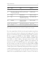
Lefebvre, 1995; Zomer et al., 2009]. Some of the figures present in the literature are
summarized in Table 1. The approach used by Zomer et al. [2009] appears to be the
most comprehensive attempt to estimate global agroforestry cover. Using 1 km resolution
data, they conclude that agroforestry involves 46% of all agricultural land. One
highlighted problem is that agroforestry systems are difficult to classify through remote
sensing because they are composed by different plant species and have different
vegetation structures, which in turn leads to very different spectral reflectance values. In
spite of this, their spatial importance cannot be neglected.
Chapter 1 Introduction
2
Mln ha
Region
Notes
Reference
8
South and South-East Asia
Homegardens
[Kumar, 2006]
45
India, Indonesia, Mali, Niger, Different agroforestry types
[IAASTD, 2008]
45
Europe
Silvoarable land
[Reisner et al., 2007]
235
USA
Alleycropping, silvo-pasture,
[Nair and Nair, 2003]
823
worldwide
Silvopasture (516 ha)+
[Nair et al., 2009]
585-1215 Africa, Asia, Americas
Agrosilvopastoral +agroforestry
[Dixon, 1995]
1000
Tree cover >10% agricultural land [Zomer et al., 2009]
C. America, Spain, Portugal
worldwide
windbreaks and riparian buffers
agroforestry (307 ha)
Table 1: Agroforestry extend estimates found in the literature for different regions of the globe.
Due to the conceptual frame of this thesis versus the spectral complexity of agroforestry,
the focus of this research is limited to coffee-banana mixed cropping systems. The main
objective is to classify land use and cover (LUC) paying special attention to agroforestry.
We will use imagery from MASTER, the airborne MODIS / ASTER simulator
developed by NASA for calibration of the spaceborne MODIS and ASTER satellite
sensors [Hook et al., 2001]. In addition, a high spatial resolution GeoEye-1 satellite
scene will serve as complement for calibration, validation, visual interpretation and
orientation in the field. As the MASTER images have a spatial resolution of approx.
10m and 25 bands in the visible near and short wave infrared (VNIR and SWIR)
spectral range of the electromagnetic solar spectrum, a second objective is to test whether
a medium spatial resolution complemented with high spectral resolution imaging sensor
is capable to identify agroforestry systems. In fact, whereas high spatial resolution sensors
are very powerful in identifying land cover and single objects on the ground, low and
medium sensors may potentially allow best inference on land use as they take into
Chapter 1 Introduction
3
account spectral information from a larger surface [Clevers et al., 2004; Franklin and
Wulder, 2002].
The pilot study site is located near Turrialba, Costa Rica. Coffee (Coffea spp.) and
bananas (Musa spp.) are respectively the first and the third cash crops in the country for
land use and production value [FAO, 2003]. In addition bananas and plantains represent
important stable food for locals and are commonly integrated in home gardens
[Montagnini, 2006; Pocasangre et al., 2011]. The association of trees to small and
medium scale coffee-banana farms is common, as it provides additional income to the
producers, relieves the exposure of crops to pest diseases and contributes to maintain soil
fertility [Lagemann and Heuveldop, 1983].
However along with these facts small and medium scale coffee-banana producers face
several challenges, namely fluctuating market prices, competition and diseases which
particularly affect indigenous cultivars. One dramatic example is the so called Panama
disease (Fusarium oxysporum cubense, FOC), a fungi which spread in the first half of 20 th
century across Central America and swept away entire banana plantations of the 'Gros
Michel' cultivar [Ploetz et al., 1999 & 2009; Blomme et al., 2011]. Export-oriented
farms rapidly switched to banana cultivars not affected by FOC, like Cavendish. But
among locals Gros Michel is still highly preferred for paid price, taste and storage quality
[Pocasangre et al., 2009]. As the fungi affects mainly production rather than plant
survival, many small-medium scale producers maintain Gros Michel in their farms
mixed with other crops in the hope of a near future eradication of the problem.
To promote conservation, profitability and development of coffee-banana agroforestry
systems in Latin America, a project called “Mejorando la producción y mercadeo de bananos
en cafetales con árboles de pequeños productores”1 was initiated in March 2009. The project,
coordinated by Bioversity International and funded by GIZ (Deutsche Gesellschaft für
1 “Improving small farm production and marketing of bananas under trees”.
Chapter 1 Introduction
4
Internationale Zusammenarbeit), has study sites in Costa Rica, Honduras, Nicaragua
and Peru. In the specific case of Costa Rica the partners can also benefit from the
facilities and support of CATIE (Centro Agronómico Tropical de Investigación y
Enseñanza) research centre.
Within this international project the Chair of Forest Inventory and Remote Sensing,
University of Göttingen was contacted with the goal of mapping FOC distribution in
the 4 study sites. As small contribution, this thesis aims at delineating an efficient
methodology to identify coffee-banana agroforestry systems using available remotely
sensed images. Though this has to be considered just a pilot study, we hope that the
blazed trails will serve as backbone and inspiration for further study developments in
land cover and FOC mapping.
In detail the objectives of this thesis are:
•
Find an effective methodology for agroforestry and LUC classification for the
study site around Turrialba with the given resources;
•
test the suitability of a MASTER scene at 10 m spatial resolution and 25 visiblenear infrared (VNIR) and short wave infrared (SWIR) spectral bands to classify
agroforestry and other land uses;
•
develop a simple and concise protocol for field data collection of reference areas;
•
profiling an applicable classification scheme and legend;
•
evaluate the accuracy and handiness of several unsupervised and supervised
classification algorithms (namely Gaussian Mixture, Maximum Likelihood and
Support Vector Machine) in the context of this study;
•
evaluate the advantage of atmospheric correction and feature selection for the
purpose of classification.
Chapter 2 Study site
5
2 Study site
2.1 Location
The study area is located in the central highlands of Costa Rica, approximately 50 km
East of San José (Fig. 3 on page 10). The frame of 7 x 7 km includes the city of Turrialba
and the research institute of CATIE.
2.2 Climate
The annual precipitation in Turrialba is about 2600 mm, prevalently concentrated
between June and December. March is the driest month with <100 mm rainfall.
Precipitation usually exceeds evapotranspiration and relative humidity is above 85%
throughout the year. The mean annual temperature is 21.5°C with limited excursion
[Kass et al., 1995; FAOCLIM data from Fuchs et al., 2010]. Because of these
characteristics the area is classified in the Köppen-Geiger eco-climate scale as equatorial
rainforest, fully humid [updated version for the second half of 20 th century by Kottek et
al., 2006]. Like in other parts of Costa Rica, movements of air masses are influenced by
land topography, which is briefly outlined below.
2.3 Geomorphology
The geological origin of Costa Rica is rather recent, being until 3 millions years ago just
a volcanic archipelago [Coates et al., 1992]. Specifically, the Turrialba valley was formed
by the Rio Reventazón which eroded the substrate formed by the volcanoes Turrialba
and Irazú [Kass et al.,1995]. The predominant soil types are Eutric Cambisol and
Umbric Andosol2 (from alluvial and volcanic origin respectively). Both substrates are
2 Nomenclature according to the World Reference Base for Soil Resources [FAO, 2006]. In soil
taxonomy they are called Andic Eutropept and Acrudoxic Melanudand respectively. Eutric Cambisol is
very deep, moderately well to well drained dark brown gravelly clay loam with larger stones in the
subsoil. Umbric Andosol is very deep, well drained dark brown clay soil, usually located on slopes
>25%. The thick A and BC layers are influenced by volcanic ashes and are highly acidic.
Chapter 2 Study site
6
fertile and can be cropped easily with small addition of P and N. Lime is sometimes
required for Andosols [Kass et al.,1995].
The study site altitude lays between 475 msl and 1225 msl, with an average of 768 msl
(data obtained from DEM, chapter 3.4). Slopes are pronounced in some areas, though
the average inclination is just 11° (20%).
2.4 Land use
The area has a good range of land cover types, which span from urban areas to forest.
Agriculture is the leading activity and this provides several examples of cropping land
use for spectral detection.
Little to none original vegetation is left due to slash and burn activities practiced since
3000 years. Maize, cultivated under shifting rotation, constituted the staple crop of
indigenous populations; wheat, sugar cane, plantains and cattle were introduced after the
Spanish reached Cartago in 1563. In the 19 th century coffee became the dominant crop
and, together with sugar cane, is still at the top of Turrialba agricultural production [Kass
et al.,1995].
Coffee is usually grown under shade trees like laurel (Cordia alliodora) and/or poró
(Erythrina poeppigiana) and mixed with Musa spp.. Laurel is native to Costa Rica and its
wood is highly appreciated on the market [Butterfield and Mariano, 1995]. Poró has
been introduced in the 19th-20th century from South America and is mainly used to
supplement nitrogen fixation in the soil [Russo and Budowski, 1986]. These mixed
agroforestry systems are reported in Costa Rica since the early 20 th century [Cook,
1901], although we would like to stress the fact that agroforestry system as defined above
are virtually impossible to date precisely back in time [Miller and Nair, 2006].
Chapter 3 Material
7
3 Material
3.1 MASTER images
3.1.1 Instrument and data description
The data used in this study to perform the LUC classification were acquired by the
MASTER imaging sensor (Fig. 1). MASTER is the MODIS/ASTER airborne
simulator developed from the joint effort of the NASA Ames Research Center, the Jet
Propulsion Laboratory and the EROS Data Center. The main objectives of this
cooperation were the elaboration of algorithms, calibration and validation of data for
MODIS3 and ASTER4, spaceborne sensors flying on the Terra platform [NASA, 2008].
MASTER
scanning
radiometer
records
radiance data in 50 spectral bands , from the
5
VNIR (visible near infrared) to the TIR
(thermal
infrared)
regions
of
the
electromagnetic spectrum (Table 2). The
channel position has been designed to
simulate at best both ASTER and MODIS
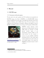
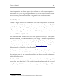
Fig. 1: MASTER camera. Image from
http://asapdata.arc.nasa.gov/Image.htm. A full
description of the optical and electronic systems
is provided by Hook et al. [2001].
measurements (Fig. 2). The ground spatial
resolution depends on the terrain surface and
on the flying altitude of the aircraft. For
MASTER it normally lies between 5 and 50
m (Table 3).
3 MODIS: Moderate Resolution Imaging Spectroradiometer.
4 ASTER: Advanced Spaceborne Thermal Emission and Reflection Radiometer.
5 Stored at 16-bits resolution.
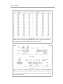
Chapter 3 Material
Table 2: Spectral characteristics of MASTER channels. On the left (channels 1-25):
VNIR and short-wavelength infrared (SWIR) band definition. On the right (channel 2650): mid-thermal infrared (mid-TIR). Table from Hook et al.[2001].
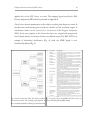
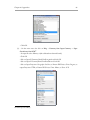
Fig. 2: Channels and wavelength regions of the MODIS, ASTER and MASTER
radiometers. (a) reflective channels, (b) thermal channels. Boxes represent the bandwidth
for each sensor channel. The numbers refer to the band numbers for each sensor. Image
from Li and Moon [2004].
8
Chapter 3 Material
9
A full description of MASTER
optical and electronic devices is given
by Hook et al. [2001]. They also
provide specific information about inflight calibration depending on the
utilized aircraft platform. Spectral
and
radiometric
calibration
of
channels is performed on a regular
basis pre- and postflight (see Arnold
et al. [1996] for procedure details).
Examples for MASTER data can be
ordered free of charge from the
NASA Jet Propulsion Laboratory
website
<http://masterweb.jpl.nasa.gov/>, at a
Table 3: Summary of MASTER sensor characteristics.
B200, DC-8 and ER-2 refer to different aircraft models
used by NASA. Table from Hook et al. [2001].
maximum of 5 scenes per order. They are compiled as Level-1B product, which means
that data are already available in radiance-at-sensor values and contain ancillary
information about geo-location, navigation and calibration [Eurimage, 2011]. MASTER
data are stored in the Hierarchical Data Format (HDF4).
3.1.2 CARTA mission
Costa Rican Airborne Research and Technology Applications (CARTA) missions are a
cooperation between the Centro Nacional de Alta Tecnologia (CENAT) and NASA.
The main objectives are the acquisition of airborne images of Costa Rica for national use
and scientific research. Until now there have been two CARTA missions, one in 2003
and one in 2005. In both these occasions four sensors have been used to collect digital
scanner data and and analogue airphotos: MASTER airborne simulator, Leica RC-30
metric camera, Cirrus Digital Camera System (DCS) and HyMap hyperspectral scanner
[ISDA, 2011]. These information about the CARTA mission are provided here as
Chapter 3 Material
10
context background and as sparkle for further sensor comparison studies.
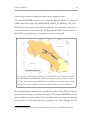
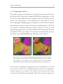
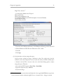
The selected MASTER image for this research was taken on March 11 th during the
CARTA 2005 mission (tile code: MASTERL1B_0500311_04_20050307_1516_1543_
V01) (Fig. 3). As the study site was fully covered by this scene and without cloud cover it
was not necessary to mosaic several tiles. The High Altitude WB-57 aircraft used flew at
8438-84596 m height allowing a 10 m spatial resolution on the ground.
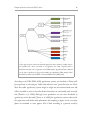
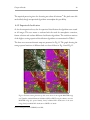
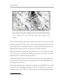
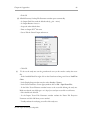
Fig. 3: Study site indicated by the red frame (7× 7 km) around the city of Turrialba, Costa Rica.
The MASTER tile (MASTERL1B_0500311_04_20050307_1516_1543_V01) from March
11th, 2005 was georectified using ENVI. Tile swath width: 14.2 km; scanline length: 200 km.
Grid projection system: UTM Zone 17N, Datum: WGS-84. Map produced in ArcMap 10.0.
Seasonal phenological variation can be a problem for remote sensing LUC classification,
especially when focusing on natural environments. The selected MASTER scene was
taken in March, the driest month of the year, which lowers the chances of cloud and
haze presence but could also mean lower vegetation cover. Thus, although for LUC
6 Data measured with a GPS device on the aircraft and retrieved from the MASTER Header File.
Chapter 3 Material
11
visual interpretation we do not expect major problems as rarely evapotranspiration >
precipitation for a period long enough for plants to dry out in a tropical rainforest region
[Eva et al., 2004], some underestimations of vegetation cover should be accounted.
3.2 GeoEye-1 images
GeoEye-1 images were used to complement LUC visual interpretation and facilitate
orientation in the field. GeoEye-1 is a satellite launched in orbit on September 8 th, 2008
by GeoEye. It is designed and equipped with very advanced technology which allows the
highest resolution among commercial satellites. It records spectral data in one
panchromatic band (ground sampling distance, GSD=0.41m 7), one near infrared and
three visual RGB bands (GSD=1.65m).
The study site around Turrialba belongs to a scene acquired on February 5 th, 2010 (order
identifier: 20100205_16072001603031604257). This image is available for private and
unpublished works without concession through the GoogleEarth™ platform, as long as
any reproduction carries the disclaimer attributes. Alternatively the raw image in 5 bands
can be purchased through the GeoEye website (http://www.geoeye.com : GeoFuse →
Advanced search → Upload file → Open Permalink).
As the purposes of this thesis did not involve any GeoEye image analysis, simple screenshots were taken from GoogleEarth. Only at the very end a standard product covering
the considered study site was ordered for evaluation and further research developments
within the funding project.
To facilitate LUC classification a raster file was created based on the GeoEye image. 432
screen-shots were taken from 1.15 km zenith distance from the ground and mosaiced
using Photoshop CS4. This mosaic was then manually georeferenced in Quantum GIS.
7 Rounded to 0.5 m due to US Government restrictions on civilian imaging.
Chapter 3 Material
12
3.3 OpenStreetMap
OpenStreetMap (OSM) is an open source, geospatial project where geographic data are
collected and shared. The aim is to create freely editable and accessible maps of the
whole world licensed under the Creative Common Attribution-ShareAlike 2.0. This
means that it is possible for example to download spatial references such as street maps
which have been traced with in situ GPS records without the burden of legal or technical
restrictions. A very handy plug-in allows to invoke and download target OSM layers
directly from the QuantumGIS working project. The OSM layers are considered to have
generally a good degree of spatial accuracy [Haklay and Weber, 2008; Mooney et al.,
2010].
3.4 Digital elevation model
A digital elevation model (DEM) of Costa Rica with 30 m spatial resolution was
available and used to retrieve basic information such as elevation and slope when not
directly possible from the MASTER image. This DEM was produced from the ASTER
scene archive during the ASTER Global DEM (GDEM) mission [ASTER GDEM
validation team, 2009]. The GDEMs are available for download from the Earth Remote
Sensing Data Analysis Center (ERSDAC) of Japan or the NASA’s Land Processes
Distributed Active Archive Center (LP DAAC) websites.
3.5 Software programs
To perform the study the following software programs were used:
Licensed
Open source
• Adobe Photoshop CS4
• DNRGarmin 5.4.1
• ESRI ArcGIS Desktop 10.0
• EnMAP Box 1.1 (64-bit operating systems)
• ITT ENVI 4.8
• JabRef 2.6
• OpenOffice 3.1
• QuantumGIS 1.7
• R 2.13
Chapter 4 Land use and cover (LUC) classes
13
4 Land use and cover (LUC) classes
The LUC classes used in this study are a modified version of the FAO 8 land cover
classification systems (LCCSs) and IGBP9 legend. The applied modifications mainly
aim at reducing the number of classes while highlighting the prominent land features of
the study area. Before proceeding with describing the classes used, it is important to
clarify the meaning of the following terms:
Land cover: “the bio-physical cover on the Earth surface” [Di Gregorio and Jansen,
1998]. E.g.: tree, mixed shrub-tree stand, water body, bare soil.
Land use: “the arrangements, activities and inputs people undertake in a certain land
cover type to produce, change or maintain it” [Di Gregorio and Jansen, 1998]. E.g.: tree
plantation, agroforestry system, swimming pool, pit.
Legend: the list of classes resulting from the classification of a specific area, using a
defined mapping scale and data set [Di Gregorio and Jansen, 1998]. All classes should be
mutually exclusive10 and total exhaustive11 [Congalton, 1991]. Both the FAO and IGPB
use discrete classes to arrange continuous variables (such as vegetation cover) in nominal
scale [Di Gregorio and Jansen, 1998], which are suitable for discussion and comparison.
There are however also examples of legend based on continuous gradients such as the
MODIS Vegetation Continuous Fields (VCF) or AVHRR CF datasets [Schwarz and
Zimmermann, 2005; Zomer et al., 2009], which are arguably closer to reality but can be
8 FAO: Food and Agriculture Organization.
9 IGBP: International Geosphere-Biosphere Programme. Their land cover legend and map [Loveland et
al., 2000] are one of the eight used for the Global Land Cover Characteristics (GLCC) database
generated by the U.S. Geological Survey's (USGS) National Center for Earth Resources Observation
and Science (EROS), the University of Nebraska-Lincoln (UNL) and the Joint Research Center of the
European Commission.
10 Each pixel should be classified unambiguously as belonging either to one or to the other class.
11 All pixels of the study area should fall into one of the classes.
Chapter 4 Land use and cover (LUC) classes
14
applied only to few LUC classes at a time. The mapping legend used by the FAO
Forestry department [FRA, 2010] is presented in Appendix A.
Classification: abstract representation of the reality as resulting from diagnostic criteria. It
describes both the discerning rules used by the classifier and the associated outputs. A
classification scheme can be hierarchical or non-hierarchical [Di Gregorio and Jansen,
1998]. As the term explains, in the former the classes are assigned with progressively
level of detail, whereas in the latter all classes are defined at once. The FAO LCCS is an
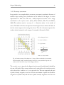
example of hierarchical classification (Fig. 4), while the IGBP legend is nonhierarchically defined (Fig. 5).
Fig. 4: LCCS used by the FAO. The scheme resembles Fig. 5: Legend used in the IGBP LCCS. The classes are
the hierarchical order. The resulting legend depends on non-hierarchically defined [FRA, 2000a].
the accomplished detail level [DiGregorio &Jansen,1998]
Chapter 4 Land use and cover (LUC) classes
15
Now that the terms land cover/use became familiar and these two officially recognized
classification schemes were briefly introduced, it is possible to speculate that the FAO
distinction between 'cultivated/managed areas' and 'natural vegetation' or the IGPB
definition of 'cropland' do involve some sort of land use knowledge. However, far from
debating here this choice, in this thesis we will keep on referring to their schemes as
LCCS. We prefer anyway to include the term 'use' for our classification scheme and
legend.
Because of the objectives and smaller scale of this study, the global scale FAO and IGBP
LCCSs had to be reduced or slightly modified. The principles to design the LUC
classification scheme were:
- adhere as much as possible to the FAO and IGBP LCCSs;
- be hierarchical, in order to be easily implemented in Decision Trees12 and larger areas.
We wanted the resulting legend to be:
- applicable at the given spatial resolution;
- meaningful to fulfill the objectives (thus irrelevant classes excluded);
- site adapted (thus unobserved classes excluded).
A visual representation of the adopted classification scheme and legend are presented in
Fig. 6 and Table 4.
The distinction between tree/shrub/herbaceous life forms follows a simplified version of
Raunkiær's classification (Appendix B). The aim was to shape artificial class delineations
in a way that better resembles natural breaks. The class threshold values are inspired
either by the FAO Forest Resource Assessment report [FRA, 2010] or by the IGBP
definitions, depending on the context and objectives. Agricultural land is separated from
non-agricultural land on the basis of produced good (crop vs. wood respectively) [FRA
2000b].
12 Decision Trees are a branch of classification algorithms based on the mapping of decision rules and
relative outputs in a tree-like format, normally dichotomous.
Chapter 4 Land use and cover (LUC) classes
16
Fig. 6: LUC classification scheme applied in this study. The underlined LUC class names
on the right are those selected for the final legend; the others written in smaller font are
just possible LUC classes not found or not applied in this study. 'Vegetated land' is
defined as land with ≥10 % vegetation cover [FRA, 2000b]. 'Agricultural land' is defined
on the basis of produced crop type and excludes tree plantations [FRA, 2000a]. Other
thresholds are taken from the FAO or from the IGBP LCCSs [FRA, 2010].
According to the FAO [FRA, 2010] agroforestry systems are classified as 'Other land'
(more precisely as sub-category 'Other land with tree cover' given that trees are >10%).
Note that coffee agroforestry systems might or might not be associated with trees and
still be classified as such, as the coffee bushes themselves are occasionally used as woody
fuel [Thacher et al., 1996]. Although more speculations on tree cover thresholds in
agroforestry can be discussed [Zomer et al., 2009], the agroforestry systems observed in
the region were only shade coffee plantations, thus implying a degree of tree cover (tree
plants are estimated to cover approx. 50% of land according to a previous work by
Chapter 4 Land use and cover (LUC) classes
17
Lichtemberg [2010] on agroforestry systems at ≥3 strata in the same region)13.
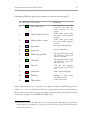
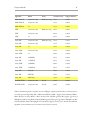
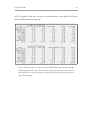
No. ID Color Class name
Definition
1
Tree crown cover
Non-agricultural area >60%
covered by the nadir tree
crown projection on the
ground.
2
Shade coffee at ≥3 strata
3
Shade coffee at 2 strata
4
Sun coffee
Sun-grown coffee plantation.
5
Sugar cane
Sugar cane plantation.
6
Mixed tree-grassland
Non-agricultural land covered
with herbaceous species and
10%≤tree cover≤60%.
7
Grassland
8
Bare soil
9
Paved road
Roads covered with asphalt.
10
Building
Buildings or other similar
man-made structures.
11
Water bodies
Coffee shrubs grown under
trees with ≥3 strata vegetation
structure.
Coffee shrubs grown under
trees with 2 strata vegetation
structure.
Non-agricultural land covered
with herbaceous species and
<10% tree cover.
Land with <10% vegetation
cover and exposed soil, sand or
rocks.
Visible surface water.
Table 4: Legend of land use and cover (LUC) classes applied to classify the MASTER image over the
study site of 7 × 7 km near Turrialba (Costa Rica) at a spatial resolution of 10 m. Agricultural land is
defined on the basis of produced crop type and excludes tree plantations [FAO, 2000b]. Other thresholds
are taken from the FAO or from the IGBP LCCSs [FRA, 2010].
13 Silvopastoral systems are included in the class 'mixed tree-grassland'. Although they are agroforestry
systems they are not considered in a separate class in this thesis due to the spectral similarity with, for
example, urban greenery.
Chapter 4 Land use and cover (LUC) classes
18
Musa spp. are often integrated in these shade coffee cropping systems. However, due to
the reduced sample size and resolution of the MASTER scene it was not possible to
infer on the presence or absence of banana and plantains in shade coffee plantations only
from remote sensing. Thus we will limit the agroforestry class definition to shade coffee
at 2 or at more vegetation strata, implying that in a 2 strata agroforestry systems there are
usually 2 species (coffee and one tree species) whereas in a system at ≥3 strata they are
usually more (coffee and several tree species and/or Musa spp.).
Cloud and shadow classes are absent in the legend. This was clear from simple visual
inspection of the MASTER image, though the decision became definitive after
evaluating the results of preliminary unsupervised classifications.
Burned land (usually sugar cane fields) could also not be detected from visual inspection
of the MASTER and GeoEye-1 images, even if likely present on the ground. Other
potential land use classes (e.g. mixed shrubs-grassland, forest clear cuts) were excluded as
no matching data were observed.
A draft of LUC classification was drawn before going to the field, though the most
suitable classes were delineated only after data collection. The FAO [Di Gregorio et al.,
1998] regards this classification scheme as a posteriori approach, like the Braun-Blanquet
system. The disadvantages of this approach are the limited application scale of the legend
on wider landscapes, site-specificity and the risk of incurring in ambiguous field notes.
However for the identification of agroforestry systems in the selected area and of specific
land use types not recognizable from the MASTER image, a posteriori classification
proved to be the most suitable. For example distinction between 'cropping land with
trees at 2' and 'at ≥3 strata' could be defined only during data collection.
Chapter 5 Methodology
19
5 Methodology
In this chapter the methodological theory applied to process and classify the MASTER
image is outlined. When needed, more technical references on the procedures are
available in the appendices.
5.1 Sampling design
When performing any classification with remote sensed resources, it is indispensable to
ensure references for the output accuracy. The references can be already validated
thematic maps, interpreted space- or airborne images, ground truth collection or a
combination of both [Plourde and Congalton, 2003; Stehman and Czaplewski, 1998]. In
this study we opted for a visual interpretation of the MASTER and GeoEye-1 image
accompanied by field data collection. The choice of the population size and sampling
design was conceived to be as efficient as possible in terms of logistic, time and financial
resources. At the same time the aim was to maintain a scientifically sound and
statistically valid approach.
The sampling design is the protocol adopted to select the observation units [Stehman
and Czaplewski, 1998]. As the majority of land use and forest inventories, the applied
sampling technique in this study is systematic sampling. This means that the location of
the observation plots follows a systematic pattern [Kleinn, 2007]. Drafting a sampling
protocol requires delineations of the population, sampling frame, sampling plot and
sampling unit, hereinafter defined.
5.1.1 Population
As mentioned in 2.1, a study area of 7 x 7 km has been selected. Having a spatial
resolution of 10 m, it is equivalent to about 490 000 pixels. This can be considered our
population, better defined as the the interest domain of the study [Kleinn, 2007].
Chapter 5 Methodology
5.1.2
20
Sampling frame
The sampling frame delimits and identifies the sample population [Stehman and
Czaplewski, 1998]. In the case of a map, a sampling frame can be areal boundaries which
include all the sampling plots.
The question on how large should the sample population be in order to fulfill a certain
accuracy confidence interval does not have an easy answer. This is why a summarized
literature review on the topic is introduced before presenting the chosen sample size for
this study.
Short literature review on sample size for remote sensed data
The following selections are mainly based on Foody et al. [2006], Tso and Mather
[2009], and Van Genderen et al. [1978]. It emerges that:
•
the sampled data must adequately represent the temporal state of the observed
phenomena, especially if the target classes are of a temporally changing nature
[Tso and Mather, 2009];
•
several authors [Atkinson, 1996; Curran, 1988; Van der Meer et al., 1999; Wang
et al. 2005; Woodcock et al., 1988] recommend the use of geostatistical methods
to choose the most appropriate sampling scheme in remote sensing because since
sampling sites have fixed locations in space their attributes are correlated and
must therefore be handled differently than standard statistical rules;
•
sample size is related to the observation scale, as the scale determines the
sampling units and thus the variability within them. For being adequate the
sample size should account for variance between classes [Tso and Mather, 2009];
•
researchers dealing with multi- and hyperspectral data should bear in mind that
the higher the number of features, the larger sample size should be in order to
maintain same accuracy degree (Hughes phenomenon [Hughes, 1968]);
•
Mather [2004] advises to equal the minimum sample size per each class to the
Chapter 5 Methodology
21
number of features multiplied by 30. He bases this figure on the notion that in
univariate statistics a sample size >30 is considered large;
•
Congalton [1991] experienced that 50 is a reasonable sample size for each
vegetation class (increased to 75-100 if the area is >1 mln acres or considering
>12 classes);
•
Van Genderen et al. [1978] propose some tables in their article to estimate the
required sample size depending on different confidence probabilities: for example
20 and 30 should be respectively the class sample size for 85% and 90% accuracy.
•
Congalton and Green [1999] propose a formula to estimate the minimum
sample size for specific confidence intervals that reflects the class multinomial
distributions14;
•
another possible approach is to base the decision on the class variance with
n=t²s²/A² where n is the sample size, t is the t-distribution, s is the standard error
and A is the confidence interval width [Foody et al., 2006; Kleinn, 2007]. This is
in line with the consideration that the model of data distribution is crucial: for
example a classifier such as Maximum Likelihood (5.4.2) requires values for the
mean vector and the variance-covariance matrix per each class to operate
effectively [Tso and Mather, 2009];
•
other statistic formulas accounting for the data distribution are discussed by
Fitzpatrick-Lins [1981] and Congalton [1991];
•
generalizing this concept, Foody et al. [2006] state that the for supervised
classification the training set size is not fixed but can vary considerably
depending on the properties of the chosen classification algorithm 15;
•
the estimations mentioned above might be severely influenced by erroneous or
unrepresentative samples included in the training set. Though the effect of
14 n = B∏i(1 - ∏i) /bi² where: n is the sample size; B the upper (α/k) × 100th percentile of the chi-square
distribution; α the required confidence lever; k the number of classes; ∏i the percentage of land covered
by class i; and b the required precision in percentage.
Chapter 5 Methodology
22
outliers should be limited for large samples, Mather [2004] presents a supportive
method to weight the observations.
Applied sample size
In spite of all these considerations, usually costs, access to sampling sites and resource
availability constrain data collection. In addition in our case no estimations on land use
could be exploited prior the actual data collection. Thus, being a pilot study, it is
acceptable to base the decision of the sample size simply on the objectives and context
constrains, postponing the evaluation of sample size adequacy to the Discussion and
Outlooks chapters.
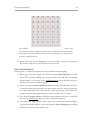
The sampling plots were distributed into 36 quadrants, each of 200 × 200 m (4 ha) and
all the surface within these quadrants was scheduled to be surveyed. The above seemed
in fact reasonable figures to cover the highest number (possibly all) land use types and
limit time and travel costs.
The systematic sampling frame was drawn as follows:
- overlay of a square grid of quadrants to the 7 x 7 km study site using a
geographical information system (GIS) software. Quadrant (grid cell) size: 200
x 200 m. Grid orientation: North-South.
- Random selection of one quadrant by the GIS software16.
- Systematic selecting other 35 quadrants at 1200 m distance17.
No slope correction was applied to these quadrants since the object of interest was the
number of pixels (which are our sampling units, see below) and not the surface area.
15 For example in the case of Maximum Likelihood (ML) supervised algorithm the mean vector and the
variance-covariance matrix per each class necessary to perform the classification influence the sample
size. For Support Vector Machine (SVM) classifier 4 very interesting strategies are proposed by Foody
et al. [2006] for improving accuracy and reducing considerably sample size.
16 In Quantum GIS©: Vector → Research Tools → Random selection.
17 Distance between any point in a quadrant and its equivalent in the adjacent quadrant =
√
49000000
36
=
√ 1361111.1111 ≈
1200m
Chapter 5 Methodology
23
5.1.3 Sampling plot and unit
Theoretically, a systematic grid should be seen as a large cluster plot made of several subplots [Kleinn, 2007]. Stehman and Czaplewski [1998] define sampling plots as all the
sites that are actually sampled. However for simplicity in this thesis we will use the terms
quadrants and sampling polygons to refer respectively to the grid sub-plots and to the
actual sampling plots. Sampling polygons were digitized on-screen within each quadrant
by partitioning the image into regions of homogeneous neighboring pixels. A LUC label
was assigned to each polygon following the legend on page 17; by doing so all the
polygon belonging pixels were also automatically labeled. For a full procedure description
see Appendix C. This process called visual interpretation was performed by one person
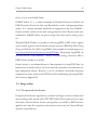
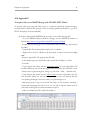
only using the georectified MASTER image and GeoEye-1 mosaic (Fig. 7).
Fig. 7: Left: one of the 36 selected sampling quadrants (red frame), whose land use classes
have been digitized and visually interpreted over MASTER-1B georectified product (RGB:
5;3;1). Right: the same quadrant over the GeoEye-1 mosaic. The colored polygons
represent different land use classes (legend on page 17). Spatial offset is discussed in 6.3.1.
Care was taken to avoid polygon overlapping. At the end of the digitization, a vector file
was created for each LUC class. The digitized polygons represent our sampling plots.
Contrary, sampling units are defined as the reference units upon which the accuracy
assessment is based [Stehman and Czaplewski, 1998]. Thus the ultimate sampling units
Chapter 5 Methodology
24
of this study are the image pixels and should not be confused with the sampling plots. If
preferred, sampling plots can be thought as spatial pixel clusters. In order to be
considered 'ground truths' the polygons need field validation [Congalton, 1991]. Due to
unavoidable human error, they will be hereinafter referred to as reference areas and not
exactly as ground truths.
5.2 Data collection
The response design defines the methodology to collect information on the LUC
reference sites [Stehman and Czaplewski, 1998]. Though in this sub-chapter only a brief
overview on the methodology is provided, a more detailed description is listed in the
field manual (Appendix I).
To validate the polygon land use on the field the followed procedure involved:
- location of the quadrant(s) position using GPS device and hard/soft maps;
- identification of the virtual boundaries of the sampling polygons;
- checking the polygon shape and assigned class value;
- registration of GPS coordinates and acquisition of digital photos from the
observation point, useful in case of doubt or as a record for future comparison.
Due to the broad class definition in the legend, it is possible to assess the class
belonging by simple visual survey of the area. If any land use change occurred between
the MASTER (2005) or the GeoEye-1 (2010) image acquisition and the field survey
(2011), we attempted to trace back to the land use in 2005 and annotate the
inconsistency.
To help data collection the used field form template is shown in Appendix D. Once the
field data collection is concluded, it is necessary to upload the land use information and
GPS points into vector layers. The digitized and field validated polygons become in this
way the regions of interest (ROIs) used as reference areas for accuracy assessment and to
train the supervised classifiers (chapter 5.4.2).
Chapter 5 Methodology
25
Data collection designed in this way can be preformed by one operator alone, though
two is the recommended number. Other equipment details are present in the field
manual. The average sampling speed, with the given location, resources and conditions,
was 4 quadrants per day. Data collection for this study was carried out in May. This field
procedure is rather economic in terms of time and money, with transportation being the
main factor to be considered.
5.3 Image processing
5.3.1 Georeferencing and subsetting the image
Once received the MASTER-1B tile in HDF format it is necessary to assign precise
coordinates to the image (georeferencing18) and subset the study area. The ENVI tutorial:
Geo-referencing images using Input Geometry provided a suitable backbone scheme for
geo-rectification, though some modifications were required (Appendix E). Note that to
follow these steps platform geometry information are necessary. In case of MASTER
products they are incorporated into the HDF file, specifically under the datasets
'PixelLatitude' and 'PixelLongitude'. After georeferencing, the MASTER image will be
overlapped with both the GeoEye-1 mosaic manually georectified and layers from
OpenStreetMap (OSM) to test the accuracy of geometric correction.
Subsetting the image was performed by overlapping the study area vector file to the
georeferenced MASTER tile. Alternatively, the exact geographic extension of the study
area can be used. The MASTER image was also spectrally subset, selecting only the first
25 visible-near infrared and short wave infrared (VNIR-SWIR) bands and excluding the
remaining 25 thermal infrared (TIR) ones. This choice was driven by the preference of
reducing data size and by the lower spatial resolution of TIR channels [Gelli and Poggi,
1999; Tso and Mather, 2009]. In addition TIR bands requires different calibration
methodologies and handling, as they record emissivity and not reflectance.
18 In this thesis the terms georeferencing and georectification will be used interchangeably.
Chapter 5 Methodology
26
5.3.2 Atmospheric correction
As indicated in Table 3, MASTER-1B products are already dispatched as 'radiance-atsensor' values; this means that digital numbers (DNs) have already been translated into
radiance values using the offset and gain metadata of instrument calibration. Radiance is
the radiant energy emitted from a particular area per unit time at a given solid angle in a
specified direction [ Jensen, 2000]. It is measured in W/(m²×sr¹). On the way to the
space, this radiant flux interacts with various atmospheric gases and particles. Thus
radiance-at-sensor indicates the radiant energy recorded by the sensor which is affected
by atmospheric scattering, absorption, reflection and refraction.
The task left to the user is to convert the radiance-at-sensor data first into true radiance
and then to reflectance. True radiance is free from atmospheric distortions which affect
radiant fluxes from the surface to the sensor. Reflectance is the dimensionless ratio
between the radiant flux emitted by a surface and the radiant flux incident to it (the sun
light) [ Jensen, 2000]. We want to evaluate if reflectance is more effective in land use
spectra characterization than radiance-at-sensor as it does not carry atmospheric
distortions and accounts for the intensity of the incoming radiating energy.
Unfortunately, measurements of atmospheric parameters are rarely associated with
remote sensed data. It is therefore necessary to retrieve their imprint on multispectral
data through the data themselves and some other known parameters. Atmospheric
correction models are able to retrieve indirectly these information and use them to
estimate the surface reflectance.
The atmospheric correction model used in this study is FLAASH (Fast Line-of-sight
Atmospheric Analysis of Spectral Hypercubes) by ITT-ENVI. FLAASH estimates
directly also the reflectance value. Its prominent features are [ITT-ENVI Atmospheric
correction module; Mattew et al., 2003]:
- wavelength correction from the visible to the SWIR (short wave infrared)
region (up to 3 µm);
Chapter 5 Methodology
27
- incorporation of MODTRAN419 radiation transfer code (this avoids using a
pre-calculated database of modeling results);
- correction of spectral mixing;
- adjustable spectral polishing parameters;
- correction of images taken from both nadir or slant positions.
The ancillary information that need to be retrieved from the Header file are the exact
day and time of flight, plane and mean ground elevation, coordinates of the scene centre,
pixel size and some climatic and geographic descriptions (tropical, rural area, etc). For a
step-by-step technical guide of the followed procedure see Appendix F. After performing
atmospheric correction with FLAASH the noisy bands will be automatically excluded
from the reflectance image.
5.3.3 Feature selection
Alternatively (or complementary) to atmospheric correction, it is possible to select the
spectral bands that are most relevant for land use class determination. Normally, noisy
bands will be discarded in this process, which is useful for reducing the size and
processing time of large spectral data sets. Two are the selection approaches taken in this
study: orthogonal transformation (PCA and MNF) and out-to-out band selection (with
R and EnMAP Toolbox). Before proceeding in describing them, few definitions are
clarified.
Spectral bands can be regarded as features, as features describe an object. Each pixel (the
objects) can thus be represented as a point in a k-dimensional plot, called feature space,
with k being the number of features [Tso and Mather, 2009]. Orthogonal transformations
transform the feature space into a new set of axes with lower correlation. These axes are
orthogonal to the originals and start at the data mean. The new number of axes can be
19 MODTRAN is a highly accurate program developed by Spectral Sciences, Inc. which models the
electromagnetic propagation of atmospheric radiation [Berk et al., 1998]. Currently, the latest available
version is MODTRAN5.
Chapter 5 Methodology
28
lower or equal to the original data set; however, since the first axes display the highest
decorrelation, it is often preferred to reduce the number of features. Orthogonally
transformed images usually appear more colorful than color composites from spectral
images because features are less correlated [Richards and Jia, 1999]. Feature selection on
the other hand does not transform the feature space but simply ranks the bands
according to their importance in determining the land use class.
Orthogonal transformations with PCA and MNF
The Principal Component Analysis (PCA) is a common technique to orthogonalize
data sets. It ranks and transforms features according to the highest variance [Richards
and Jia, 1999]. However, this does not imply that noisy bands are excluded. The
Minimum Noise Fraction (MNF) transformation overcomes this problem by generating
feature spaces that maximize the signal-to-noise ratio [Canty, 2010]. It is actually a
double Principal Component transformation where first noise is isolated and rescaled
and in the second step the remaining bands are regularly processed as in a PCA [ITTENVI, 2001].
Performing PCA and MNF transformations is a rather automatized process in ENVI
and easy to perform. In both cases it is possible to select each time a different number of
features (bands) to describe the final image. For more theoretical background on PCA
and MNF see respectively Landgrebe [1998] and Green et al. [1988].
Feature selection in R
The package used in this study from the statistical program R is randomForest™
developed by Leo Breiman and Adele Cutler [Breiman, 2001]. A technical record of the
steps follows in Appendix G. The two indexes used by randomForest to rank feature
importance are the Mean Decrease Accuracy (MDA) and the Mean Decrease Gini
(MDG). MDA ranks variables according to their difference in prediction accuracy.
MDG is the normalized sum of all Gini decreasing impurities along a tree over the total
number of trees [Calle and Urrea, 2011]. It is implicitly assumed that noisier bands will
score low in the list.
Chapter 5 Methodology
29
Feature selection with EnMAP Toolbox
EnMAP Toolbox 1.1 is a software developed by Humbold University of Berlin and
DLR (Deutsches Zentrum für Luft- und Raumfahrt) for multi- and hyperspectral data
analysis. It is currently developed specifically for hyperspectral data from EnMAP, a
German scientific satellite mission with envisaged launch in 2013. However with some
modifications EnMAP Toolbox can process images from other remote sensing sources
too.
Through EnMAP Toolbox it is possible to invoke imageSVM, an IDL tool for support
vector machine regression and classification analysis based on LIBSVM by Chih-Chung
Chang and Chih-Jen Lin [2011]. imageSVM is freely available for scientific purposes at:
http://www2.hu-berlin.de/hurs/projects/imageSVM.php. Alternatively, imageSVM can
run from the IDL Virtual Machine™ without necessarily owning a license for IDL or
ENVI [Van der Linden et al., 2010a].
Feature selection is an indispensable part of data preparation in imageSVM. Since the
band selection is mainly based on visual assessment, this method has some limitations for
large hyperspectral datasets. However, it can be considered a potentially interesting
complement to feature selection with ENVI and R. For familiarizing with imageSVM in
this context see Appendix H.
5.4 Image analysis
5.4.1 Unsupervised classification
Unsupervised classification algorithms use statistical techniques to cluster k-dimensional
data according to their spectral values [ITT-ENVI, 2001]. They require the user to input
the number of desired clusters. Several such algorithms are available in ENVI and were
applied in this study. For compactness and relevance reasons only the Gaussian Mixture
algorithm is presented here.
Chapter 5 Methodology
30
Gaussian Mixture
The Gaussian Mixture is an iterative algorithm somehow superior to other unsupervised
classification methods because it uses multivariate normal probability densities, thus
allowing higher clustering flexibility [Canty, 2010]. This classification tool is only
available in ENVI with the IDL extension. The algorithm used in this study is actually
Canty's modified version of Expectation Maximization (EM) applied to a Gaussian
Mixture model. Unfortunately this extension is not suited for large or high-dimensional
data sets because it does not exploit the ENVI tiling facility; it allows though a more
flexible algorithm parametrization.
5.4.2 Supervised classification
Contrary, supervised classification requires the user to select and input training areas,
which are used to train the classifier. Though the procedure might be tedious, the results
are ofter more satisfactory than those from unsupervised classification [Tso and Mather,
2009]. The disadvantage is that for defining the classes some prior knowledge on the
study site is necessary.
Like for unsupervised classification, ENVI offers several options as algorithms. The two
that gave the most promising results in this study are the Maximum Likelihood (ML)
and the Support Vector Machine (SVM), which were implemented into 5 variants:
standard ML and SVM in ENVI, ML and SVM with accuracy assessment modified by
Canty [Canty, 2010] and SVM in EnMAP Toolbox.
Maximum Likelihood
The Maximum Likelihood classifier ranks the pixel belonging probability to each class
and assigns the pixel to the class with the highest probability [Tso and Mather, 2009].
This assignation is based on the reflectance value or digital number per each band. ML
classifier assumes that all classes have a normal probability distribution prior band
analysis. However, developments of this algorithm not applied in this study proved that
there is the potential to use expected class distribution or pixel context to improve the
final ML classification accuracy [Strahler, 1980; Hubert-Moy et al., 2001].
Chapter 5 Methodology
31
The decision rule used by ENVI ML classifier is [Canty, 2010; Richards and Jia, 1999]:
pixel g is in class i provided di(g) ≥ dj(g) for all j = 1 ... I
given that the discriminant function is:
di(g) = -log|
The moments
−1
∑i | - (g – µi)t ∑i (g – µi)
∑i and µi are directly estimated from the training data.
Due to the limited number of parameters estimations, the computational time is also
limited [Canty, 2010]. Being a parametric model, ML strongly relies on the prior
assumption of data structure. If the normal distribution assumption is correct, parametric
models show stronger results as compared to non-parametric ones [Whitley and Ball,
2002].
ML classification in ENVI outputs also a gray-scale rule image consisting of the
discriminant functions for each class and training observation [Canty, 2010]. In the case
of ML the rule image values are the probability of pixel belonging to class. This rule
image can be used to evaluate the classification and possibly to modify the discriminant
thresholds [ITT-ENVI Tutorial: Classification methods; ITT-ENVI, 1999].
Support Vector Machine
Support Vector Machine (SVM) classifiers are state-of-the-art machine learning
algorithms [Tso and Mather, 2010]. Like in ML methods, the structural
misclassification error is minimized by accounting for data variance. But whereas in ML
the variance is empirically estimated, SVM partitions the feature space by taking a subset
of the training data (the support vectors) without invoking their distribution [Canty,
2010]. Being a non-parametric model, SVM has the advantage to fit well most data sets
[Whitley and Ball, 2002]. Though SVMs were originally conceived for binary
classification, a number of multiclass applications have been investigated [Hsu and Lin,
2002; Huang et al., 2002; Foody and Mathur, 2004]. The multiclass approach used in
ENVI to determine the membership class is regarded as a 'one-to-one' voting scheme
[Canty, 2010].
Chapter 5 Methodology
32
SVM with EnMAP Toolbox
With EnMAP Toolbox-imageSVM described on page 29 is possible to classify an image
using the SVM algorithm. Though the results should be very similar to SVMs applied in
ENVI, in reality different adjustable model parameters can originate different outputs. In
particular the user can modify the width of the Gaussian kernel function (parameter g in
K(x, xi) = exp(-g |x-xi|²) used to separate class distribution and control the training data
individual influence (C) on classification [van der Linden et al., 2010a].
ML and SVM by Canty
In addition to standard ML and SVM classification methods, also a modified version of
both was applied. Canty [2010] in fact developed some ENVI/IDL extensions for
standard classifications with a smart consideration for accuracy assessment.
Normally, the confusion matrix (chapter 5.4.3) is used to evaluate the classified map
accuracy. ENVI built-in procedure:
•
uses pixels from all training areas to calculate average band values per each class;
•
these averages are used to classify the whole image (note: it can be that the final
classification of some training pixels differs from the original assigned class);
•
the confusion matrix is calculated by taking pixels from these training areas and
compare them with the final classification.
Whereas Canty's variants:
•
separate the pixels of all training areas into training and testing sets (in
proportion 2:1);
•
take the average band values of the training set to classify the whole image;
•
the confusion matrix is calculated by comparing the testing pixels with the final
classification.
Clearly the advantage of Canty's variant lays in the fact the testing pixels are completely
independent from the training one, therefore the assessment is less bias.
Canty's ENVI/IDL extensions can be downloaded for free from his webpage
(http://mcanty.homepage.t-online.de/software.html ).
Chapter 5 Methodology
33
5.4.3 Accuracy assessment
Image analysis is not complete before an accuracy assessment is performed. Accuracy of
thematic maps resulting from classification can be defined as the degree of correct
representation of land cover. The most
widely accepted assessment tool in image
classification is the confusion matrix [Canty, 2010; Stehman, 1992; Tso and Mather,
2009]. The confusion matrix is an array of i × i dimension where i is the number of
classes. The labels in the first row represent the training data classes whereas the labels in
the first column represent the testing data classes. The cells in between represent the
number of pixels assigned to each category. An example is illustrated in Fig. 8.
OA = Σ diagonal / total
Pi = (i, i) / Σ column i
Ui = (i, i) / Σ row i
5
κ=
(OA−∑ P i ×U i )
i=1
5
∑ ( P i ×U i )
i=1
where i is a class number
Fig. 8: Confusion matrix of classification at 5 classes. Cells are indicated as: (row number,
column number). P and U stand for Producer's and User's accuracy with the respective class
number, OA for Overall Accuracy. K is the Kappa coefficient.
The overall accuracy is given by the diagonal sum (correctly classified pixels) divided by
the sum of all pixels. Other accuracy indexes can be retrieved from the confusion matrix,
such as the producer's and the user's accuracy per each class. These are respectively the ratio
of pixels correctly assigned to one class over the total number of pixels that should be
assigned to it (column sum) and the ratio of pixels correctly assigned to one class over
Chapter 5 Methodology
34
the total number of pixels that were assigned to it (row sum) [Tso and Mather, 2009].
Last but not least, from the confusion matrix it is possible to calculate the Kappa
coefficient. Contrary to the producer's and user's accuracy, the Kappa coefficient κ takes
into consideration all the information contained in the confusion matrix and corrects the
classification rate for the probability of classifying pixels correctly by chance [Canty,
2010]. Alternatively to the equation given in Fig. 8 κ can be defined as:
κ=
Pr (correct classification)−Pr (chance classification)
1−Pr (chance classification)
where Pr stands for probability [Tso and Mather, 2009]. κ is considered somehow more
accurate than other indexes because provides two statistical tests of significance into one.
It indicates in fact
the degree of significant difference between the result of the
classification and a random classification. Second, it can be used as reference for
comparing two matrices, as in the case of classification algorithm evaluation. Although
Stehman [1992] points that κ could slightly lose its assessing power when used in
context other than simple random sampling, other authors [Congalton and Green, 1999;
Foody, 2000; Li and Moon, 2004] used it for accuracy assessment also in systematic
sampling. The confusion matrix accuracy assessment can be applied to both supervised
and unsupervised classifications. Instead of the confusion matrix, it is possible to obtain
an accuracy assessment also by reiteratively repeat the 'leave-one-out' test [Gretton et al.,
2001; Kearns and Ron, 1999] (not applied in this study, though).
5.5 Post-classification processing
Some post-classification tools in ENVI can be used to improve the accuracy. These
functions are named Sieve, Clump and Combine Classes. Sieve smooths the image by
removing isolated pixels, after a minimum cluster size has been input. Clump merges
similarity classified areas. Combine classes allows the user to join classes with very similar
spectra into a more generalized one [ITT-ENVI Tutorial: Classification methods].
When appropriate, all three tools were tested over the classification results.
Chapter 6 Results
35
6 Results
6.1 Sampling design
A total of 207 sampling plots were digitized, belonging to 12 land use and cover classes.
The number of selected reference pixels was 14 842 over a population of 490 000.
6.2 Data collection
198 polygons were actually field validated as the remaining 9 sites could not be accessed,
leaving a total of 13 744 pixels to be used as reference areas. During field data collection
the LUC labeling of 38 polygons and the shape of 17 ones was modified due to visual
misinterpretation of the remote sensed images. The most commonly misattributed LUC
classes from visual interpretation compared with field survey were: mixed tree-grassland
(15), shade coffee at ≥3 strata (13), shade coffee at 2 strata (7). The LUC type changed in
only in two sites between 2005 and 2011; it was anyway possible to trace back to the
original land use, being mainly agricultural fields under crop or fallow rotation.
All GPS point and digital pictures acquired during data collection were incorporated
into vector files using the QuantumGIS-eVis plugin (Appendix C).
6.3 Image processing
6.3.1 Georeferencing
The maximum observed spatial offsets between the georectified MASTER against the
OpenStreetMap (OSM) layer and GeoEye1 mosaic were ±3 and ±4 pixels (30 and 40 m)
respectively (Fig. 9). Surprisingly, the spatial offset between the GeoEye-1 manually
georeferenced mosaic and the OSM layer was 10-15 m, lower than the dispatched
original 5 band GeoEye-1 image (~20 m offset against OSM). On the other hand
orthorectification of the GeoEye-1 standard product with the available DEM using
ENVI 4.8 improved the spatial accuracy to ± 5-7 m.
Chapter 6 Results
36
Fig. 9: MASTER image (left) and GeoEye-1 mosaic (right) overlayed with
OpenStreetMap (OSM) layer.
6.3.2 Atmospheric correction
From FLAASH one reflectance image was created and scaled for a factor of 10 000
(Appendix F). A sample spectra profile of the reflectance image compared to the original
radiance-at-sensor is shown in Fig. 10. The 3 bands automatically excluded by
FLAASH because classified as noisy were band 16, 17 and 18 (1.78 to 1.98 µm).
Fig. 10: Radiance (left) and FLAASH-reflectance (right) images of MASTER scene over
Turrialba. The associated spectral profile refer to the same pixel. Index = band number.
Chapter 6 Results
37
6.3.3 Feature selection
From PCA and MNF analysis three images have been created: one PCA at 4 bands and
two MNF at 6 and 25 bands respectively. The number of bands is subjectively chosen by
the operator. However the aim was to condensate spectral information while preserving
essential traits for classification.
The R-randomForest MDA and MDG ranking results are shown in Fig. 11.
Fig. 11: Feature selection using the Mean Decrease Accuracy (MDA) and the Mean Decrease
Gini (MDG) indexes available in R randomForest package. The bands (B) are ranked top-tobottom according to the importance in determining the LUC class. Only 22 bands appear in
each list, as the other 3 (23 to 25 in both cases) were considered less influential thus excluded.
This forest was obtained using the first 25 bands of MASTER data, set seed= 4543, trees = 1000.
Chapter 6 Results
38
From these rankings the first 16 (MDA > 0.38) and 17 (MDG > 450) bands were
selected. This means that the bands used for further processing from MDA index were
all except 13 to 15, 18 to 20 and 23 to 25; and for the MDG index all except 16, 18 to 20
and 22 to 25.
Last, as mentioned in 5.3.3, EnMAP Toolbox does not provide a statistical comparison
among bands. However EnMAP Toolbox (like ENVI on the other hand) offers the
possibility of identify noisy bands by visual interpretation. A screen-shot with one
significant band and the three noisy ones is presented in Fig. 12.
Fig. 12: Screen shot of 4 MASTER spectral bands displayed in EnMAP Toolbox.
Clockwise from top left corner: band 3, 16, 17 and 18. The image is MASTER-1B (March,
11th 2005) over the study site in Turrialba, Costa Rica.
Only these 3 bands (16, 17 and 18) were classified as noisy in EnMAP Toolbox .
Chapter 6 Results
39
6.4 Image analysis
6.4.1 Results of unsupervised classification
The Gaussian Mixture algorithm could be applied only to images with reduced number
of features. Therefore the algorithm was only tested on: PCA at 4 bands, MNF at 6
bands, first 5 bands of the radiance-at-sensor image and first 5 bands of the reflectance
image20. The used parameters were: initial number of classes = 11; min threshold = 0 max
threshold = 2. The output clusters were visually analyzed and confronted with the true
color composite MASTER image and other thematic from supervised classification
maps to facilitate interpretation; a land use label was assigned to the clusters, which in
some cases were merged. The results were then tested in a confusion matrix against the
reference ROIs created in 5.1.3. Note that only the identified LUC classes could be
tested in the confusion matrix; this mean that each time a different number of test pixels
was considered. The overall accuracies of these 4 Gaussian Mixture classifications and
the relative Kappa coefficients are listed in Table 5.
Image
No. bands
No. classes
No. tested pixels
OA
Kappa coeff.
PCA
4
8
13339
46.4%
0.3732
MNF
6
8
12951
54.2%
0.4578
Radiance-at-sensor
5
7
12728
53.5%
0.4111
Reflectance
5
9
13562
42.8%
0.3210
Table 5: Overall accuracies (OA) and Kappa coefficients obtained from confusion matrices of 4 images
classified with the Canty's modified version of Gaussian Mixture algorithm. No. classes indicates the total
number of classes after merging and labeling tested in the confusion matrix. No. tested pixels indicates the
total number of pixels from the reference ROIs which were used in the comparison. Initial parameters:
number of classes = 11; min threshold = 0 max threshold = 2.
20 The algorithm can be applied only to floating-point images and not to the 2-byte integer scaled
reflectance.
Chapter 6 Results
40
The required processing time for clustering was above 60 minutes 21. No pixels were left
unclassified, though unsupervised algorithms contemplate this possibility.
6.4.2 Supervised classification
As for the unsupervised case, also for supervised classification the algorithms were tested
on all images. This was meant to evaluate both the need for atmospheric correction,
feature selection and evaluate different classification algorithms. The confusion matrices
of the highest scoring supervised classification algorithms are summarized in Table 6.
The three most accurate thematic maps are presented in Fig. 13. The graph showing the
average spectral emission of different land use classes follows in Fig. 14 and Fig. 15.
Fig. 13: Clockwise starting from the top left corner subset of: the original MASTER image
over Turrialba; standard Maximum Likelihood (ML) in ENVI using the radiance-at-sensor
MASTER image (25 spectral bands); Canty's modified ML classification of the same
image; Canty's modified ML classification of MNF at 25 bands.
21 In a 32-bit processor, 2 GB RAM, 2.16 GHz.
Chapter 6 Results
41
Algorithm
Bands
Notes
Overall accuracy
Kappa coefficient
MaxLikelihood
22 (no 16 to 18)
Reflectance img
70.0%
0.6432
MaxLikelihood
22 (no 16 to 18)
71.7%
0.6638
MaxLikelihood
25
73.5%
0.6841
SVM
22 (no 16 to 18)
68.0%
0.6085
SVM
22 (no 16 to 18)
68.3%
0.6109
SVM
25
68.5%
0.6144
Canty ML
22 (no 16 to 18)
71.1%
0.6558
Canty ML
22 (no 16 to 18)
71.3%
0.6588
Canty ML
25
73.1%
0.6794
Canty SVM
22 (no 16 to 18)
67.5%
0.6016
Canty SVM
25
67.6%
0.6024
Canty ML
16 (MDA)
67.7%
0.6182
Canty ML
17 (MDG)
69.3%
0.6364
Canty SVM
16 (MDA)
66.6%
0.5906
Canty SVM
17 (MDG)
66.3%
0.5872
Canty ML
PCA (4)
48.8%
0.4199
Canty ML
MNF (6)
59.0%
0.5223
Canty ML
MNF (25)
73.1%
0.6789
En-MAP SVM
22 (no 16 to 18)
See (a)
71.1%
0.6790
En-MAP SVM
22 (no 16 to 18)
See (b)
64.6%
0.6069
Reflectance img
Reflectance img
Table 6: Summarizing table of overall accuracies and Kappa coefficients obtained from confusion matrices
of several supervised algorithms. ML = Maximum Likelihood, SVM = Support Vector Machine, MDA =
Mean Decrease Accuracy, MDG = Mean decrease Gini. (a) Min (g)=0.01; Max (g)=10; (g) and (C)
Multipliers=2; Min (C)=1; Max(C)=10000. (b) Min (g)=0.01; Max (g)=1; (g) and (C) Multipliers=2; Min
(C)=100; Max(C)=10000. The highlight rows indicates the highest accuracy scores. Results from different
algorithm / band combination are not shown because of lower accuracies.
Chapter 6 Results
Fig. 14: Average land use class spectra of reference ROIs associated with MASTER
radiance-at-sensor image (25 bands). Line colors correspond to the legend on page 17.
Unit of the x-axis: wavelength (µm); y-axis: radiance (W m-2 sr-1).
Fig. 15: Average land use class spectra of reference ROIs associated with MASTER
FLAASH-reflectance image (22 bands). Line colors correspond to the legend defined
on page 17. Unit of the x-axis: wavelength (µm); y-axis: reflectance ratio.
42
Chapter 6 Results
43
If we consider the computational effort PCA at 4 bands, MNF at 6 and 25 bands
transformed images took in general slightly less time for classification processing as
compared to the MASTER image at 22 and 25 bands in all classification algorithms.
Time difference was more pronounced among algorithm types, with SVM classification
being the slowest (approximately 30 minutes in ENVI vs about 1-2 minutes for ML)22.
However SVM processing time in EnMAP Toolbox highly varied depending on the
input parameters (especially sampling type, g and C). For the tested combinations it was
in the range of 3 to 200 minutes23.
6.5 Post-classification processing
The 3 most accurate classification images were first sieved and then clumped. The
respective accuracy assessment results are presented in Table 7.
Algorithm
Image
Tool
Overall acc.
Kappa coef.
ML
MASTER 25 bands
sieve
72.7%
0.6765
clump
74.8%
0.7002
sieve
72.3%
0.6712
clump
73.8%
0.6889
sieve
72.2%
0.6706
clump
73.8%
0.6887
Canty ML
MNF 25 bands
Table 7: Overall accuracies and Kappa coefficients of 3 post-classified images. ML stands for Maximum
Likelihood. MNF 25 for Minimum Noise Fraction at 25 bands. Clump was performed on the sieved
image. Sieving parameters: 2 min. threshold, 8 number of neighbors. Clumping parameters: 3 operator size
row, 3 cols. The highlight row shows the best combination in terms of accuracy.
22 In a 32-bit processor, 2 GB RAM, 2.16 GHz.
23 In a 64-bit processor, 16 GB RAM, 4 double processors.
Chapter 6 Results
44
Clumping was performed on the sieved image. In these case if clumping was performed
prior sieving directly on the MASTER classified image the final accuracy would have
been lower (results not shown). Sieving leaves some pixels unclassified; their number
decreases after clumping but does not disappear.
At last we performed Combine Classes for the best sieved and clumped output (sieving
and clumping of MASTER image classified with the standard ML algorithm). We
started by analyzing carefully the confusion matrix (Fig. 16) and rule images (Fig. 17).
Fig. 16: Confusion matrix of sieved & clumped MASTER radiance-at-sensor image (25
spectral bands) classified with ENVI ML algorithm using 11 LUC classes. The shown part
of the confusion matrix indicates the matches between the testing (column) and the training
(row) areas expressed in percentage. Overall accuracy: 74.8%; Kappa Coefficient: 0.7002.
Chapter 6 Results
45
Fig. 17: Examples of rule images resulting from ML classification of MASTER reflectance
scene. On the left: rule image of class 2 (shade coffee at ≥3 strata). On the right: rule image
of class 3 (shade coffee at 2 strata). Dark pixels indicate higher probability of class
belonging.
The class matches with less than 74.8% overall accuracy value are: tree crown cover and
mixed tree-grassland. Tree crown cover is often confused with: shade coffee at ≥3 strata
(11%), shade coffee at 2 strata (8%) and mixed tree-grassland (7%). Because the aim is to
distinguish these categories, the class tree crown cover was left untouched.
Mixed tree-grassland is misclassified with: shade coffee at 2 strata (12%), tree crown
cover (8%), sugar cane (8%) and building (6%). Since these classes have little
management use in common they were preserved too.
To reduce the number of classes the two shade coffee classes were merged together into
one class called shade coffee; and the class paved road was merged with building into a
new category called settlement.
The comparison between the combined class image and the merged ROIs 24 gives overall
accuracy of 76.7% and Kappa coefficient of 0.7127. For specific class accuracy in
percentage refer to Fig. 18. The class shade coffee was classified respectively with 86%
24 See Discussion 7.4 for details.
Chapter 6 Results
46
and 71% producer's and user's accuracy. As mentioned before, some pixels (1.4%) were
left unclassified after the sieving step.
Fig. 18: Confusion matrix of sieved and clumped MASTER image classified with ML
modified algorithm after 2 LUC classes have been merged. The shown part of the confusion
matrix indicates the matches between the testing (column) and the training (row) areas
expressed in percentage.
Chapter 7 Discussion
47
7 Discussion
7.1 Sampling design
Implementing a systematic sampling scheme has several advantages: it requires no prior
knowledge on the area; it is simple to explain to the field crew and to the reader; the
observation units are spread homogeneously over the area and thus less autocorrelated;
all parts of the population are covered, assuming that there is no cyclic land use
distribution [Kleinn, 2007]. There is however the risk of under or over-represent some
classes: for example too few reference pixels belonging to rare classes are collected to
train properly the classifier or too many energies are invested in digitizing the umpteenth
polygon which does not contribute in increasing information on that land type [Plourde
and Congalton, 2003].
Thus considering the purpose of LUC classification and the drawbacks of systematic
sampling, it could be possible to apply a stratified sampling scheme in further studies, as
it would guarantee that all land use classes are represented equally. In stratified sampling
homogeneous objects on the ground are isolated and visually classified. Object isolation
can be performed through segmentation, followed by semi-automatic classification (best
suitable for high spatial resolution images); alternatively, unsupervised classification can
also work to identify land cover with similar spectra in lower resolution products. The
selection of the objects to be sampled can be random or follow a(n) (un-)aligned scheme
[Fitzpatrick-Lins, 1981].
One disadvantage of stratified sampling is that transport logistic, plot location and
permission to access the sites might balanced out the time savings from manual polygon
digitization of the whole quadrants. In addition in the case of unsupervised clusters
labeling it is possible to perpetrate systematic observer bias if the operator is not familiar
with the study scene, thus leading again to an unbalanced number of samples per class.
However a successful implementation of stratified random sampling scheme was done
for example by Foody et al. [2006], who also suggest 4 interesting tricks to reduce sample
Chapter 7 Discussion
48
size when the focus is on one class only.
The population size of this study was not random, as 49 km² is the minimum required
area for ordered GeoEye-1 or IKONOS satellite imagery. This is an important factor to
consider if the research is extended using different sensors or sites.
The sampling grid orientation was North-South and this could be arguably objected as
user bias choice. However, if there is not a cyclic pattern in the landscape (e.g. systematic
arrangements of sugar cane fields at 1200 m distance in the North-South direction), the
error variance of the land use classes should not be much higher than from a sampling
grid randomly oriented [Kleinn, 2007]. Moreover, it is easier to visualize and explain a
systematic grid with cells oriented North-South rather than one oriented at different
azimuths. Therefore, from the trade-off between increased error variance and higher
practicality, we decided to apply a North-South orientation.
From a practical point of view the grid cell size (200 × 200 m) appeared to be suitable for
the objective of land use observation around Turrialba, as each quadrant could be easily
surveyed. However, the spectral variance among polygons of the same LUC class but
belonging to different quadrants could be statistically studied using the intracluster
correlation coefficient. This information should help in finding unconsidered spatial
autocorrelation and be potentially incorporated into a stratified sampling scheme.
A way to increase statistic accuracy might be to switch the square systematic grid to a
triangular one (this leads to a systematic unalignment of plots). Though the precision
increases as the observation points are scattered even more homogeneously over the area,
the square grid is just slightly less precise [Kleinn, 2007]. Therefore for simplicity a
square grid is often preferred.
As referred in the methodology, several are the formulas proposed in the literature to
estimate the sample size for remote sensed data within a certain confidence level. For
Mather [2004] rule of thumb 30 × 25 bands = 750 pixels should be sampled per class;
this gives a total of 8250 pixels (750 × 11 classes), below our sample size of 13 744.
Before data collection other formulas were not possible to apply as no variance
Chapter 7 Discussion
49
estimations were available. After classification it is possible to obtain statistical
information on the processed data, in particular the class standard deviation, covariance
and correlation per each band (using ENVI Class Statistics). However, due to handling
complexity of considering 25 spectral bands, spectral autocorrelation of neighboring
pixels, feature space correlation, class distribution, definition and separability and lack of
literature on the topic it was not possible to evaluate the chosen sample size or infer on
the appropriate one within this study. It would be extremely fascinating to read in the
future of studies on the topic.
Once the sampling scheme and sample size have been selected, for classification
purposes it is also important to consider the sample placement and cluster size. Plourde
and Congalton [2003] suggest to create training samples in homogeneous areas rather
than selecting larger clusters which include many mixed pixels. Testing this effect on
accuracy would be interesting by comparing our classification results with those from
new digitized sampling polygons where all the edge pixels have been discarded. When
evaluating these results it is however important to consider possible sample size
differences, as the quadrants might no longer be wholly classified.
Congalton [1988] moreover showed that the size of each training areas should not be
larger than 10 pixels, as no information is added by extra contiguous pixels. This is due to
spectral correlation and reinforces the suggestion to digitize smaller plots within the
original ones.
7.2 Data collection
The major issues faced in the field by applying the response protocol were in order: (i)
plot access and (ii) location of the sampling plot in the ground. For the former it is very
important to consider legal and security issues, as access to private land is not always
possible. Distinctive signs such as an official car or a disclaimer document should help in
most cases.
To locate more easily the plot an idea is to follow the path to reach it on a topographic
map or a digital support such as Google Earth™. It was in fact experienced during the
Chapter 7 Discussion
50
field work that access to the Google Earth platform is possible even without internet
connection, given that the program was preliminary opened roughly on the area of
interest. In this way also the zooming in/out tool remains active.
Recording the camera height as described in the field manual (Appendix I) can be time
demanding when the plots are numerous and superfluous for the objectives, so it can be
omitted in similar studies.
No error assessment [Van Genderen et al., 1978] was conceived for evaluating the
accuracy of field data, the main reason being the simplicity of the legend applied.
However it is recommended to employ at least two operators for the field data collection
in order to reduce even more chances of error in plot location and/or class attribution.
Time gap between the sensed image and the field data collection is an issue to be taken
into account. In our case, though the gap was 6 years, the land use management had not
changed much. Only one site (consisting of 2 digitized plots) was converted from
presumed pasture to tree plantation and was thus not possible to validate. In all other
instances it was mainly a seasonal change rather than a change in land use (e.g. sugar
cane fields were harvested when in the MASTER image they resulted still green or
viceversa). In such cases it is important to adhere to the image interpretation as it is the
image which will be processed.
When there is the need of assessing the usefulness of data collection, digitizing land use
polygons before going to the field could provide a valuable basis for comparison with the
field data. Considering the proportion of changed land use class (about 1 out of 5) and
polygon shape (1 out of 12), it appears clear the need for field sampling in this study.
7.3 Image processing
It is very hard if not virtually impossible to achieve 100% geospatial accuracy in a map.
Even the used OpenStreetMap (OSM) layers which were taken as spatial reference
might contain geometric inaccuracies. These can be due to the GPS receiver positional
error and/or low density of recorded points. However we assume these errors to be
Chapter 7 Discussion
51
limited as compared to automatized georectification of large images (such as the
MASTER tile) or manually georeferenced images (as in the case of the GeoEye-1
mosaic). In addition it has to be mentioned that the latter carries small overlapping
errors occurred during mosaicing. Thus the best available spatial reference were the
OSM layers.
30 and 40 m spatial offset between the MASTER and respectively the OSM layer and
GeoEye-1 mosaic indicate that there is room for geospatial improvements. On the other
hand for the purposes of this study it is possible to accept this misregistration as the only
images that were actually compared were the georeferenced MASTER image and the
deriving thematic maps (which obviously match exactly). In future studies, if land use
changes have to be detected over time, it is important to keep in mind the positional
accuracy and matching of the analyzed maps. For ideas how to improve it see chapter 9
Outlooks.
When considering larger study areas, cloud cover and haze might require tile mosaicing.
It is possible to conduct this operation with ENVI, however care should be taken when
analyzing and processing the resulting mosaic. In fact different illumination conditions
can affect further processing outputs. Therefore, in mountainous terrain with steep slopes
topographic normalization should be applied. Also, to create a more homogeneous image
it is recommended to atmospherically correct the mosaic (for example with the ENVI
extension IR-MAD25 [Canty and Nielsen, 2008] or with FLAASH model in ENVI),
with one manual method (like Empirical Line Calibration or Flat Field) and/or by
matching the image histograms using for example ERDAS-Imagine. The 'feathering'
option in ENVI [ENVI Tutorial: Mosaicking] seems in fact too simplistic and does not
solve the problem throughout but just in the overlapping area.
The described atmospheric correction models assume the Earth surface being flat and
having a Lambertian reflectance behavior [Tso and Mather, 2009]. In this way the
radiance pixel values are homogeneously corrected throughout the image, without taking
25 Interatively Re-weighted Multivariate Alteration Detection.
Chapter 7 Discussion
52
into account that different elevations and roughness of the landscape cause different
solar incident and radiance angles. Though not applied in this study, two top methods
for topographic correction are suggested: band ratioing and the Minnaert method
[Colby, 1991; Law and Nichol, 2004; Tso and Mather, 2009]. Both take into account the
satellite position as well.
Despite the promising results by Matthew et al. [2003], the reflectance image
atmospherically corrected using FLAASH did not perform better than the radiance-at-
sensor image (Table 6) and was therefore abandoned during classification. The need for
atmospheric correction of a satellite scene of one acquisition date can be called in
question if no accuracy benefits arise from it. However, a deeper analysis of the
methodology applied could reveal involuntary misuse of the model. For suggestions how
to improve the application of FLAASH see Outlooks.
In addition, other atmospheric modeling techniques could be tested, like Atmospheric
CORrection Now (ACORN) and ATmospheric REMoval (ATREM). ACORN uses
MODTRAN4 radiative transfer code like FLAASH for estimating atmospheric
parameters, but contrary to the latter it retrieves water vapor concentration using bands
0.94 and/or 1.15 µm [Kruse, 2004]. ATREM26 on the other hand is based on a 6-S
atmospheric correction code, improved by Vermote et al. [1997] and briefly discussed in
Tso and Mather [2009]. A comparison of these 3 atmospheric modeling techniques is
given by Kruse [2004].
There are some proves that empirical methods such as DOS (Dark Object Subtraction)
and ELC (Empirical Line Calibration) could perform better than theoretically superior
but generalized models in calibrating remote sensed images [for DOS see Lu et al., 2002;
for ELC see Karpouzli and Malthus, 2002], though the issue is still debated [Smith and
Milton, 1999; Mahiny and Turner, 2007]. Empirical techniques require some knowledge
of ground conditions, which have to be retrieved either from the image itself (in DOS)
or by ground measurements (also subsequent, in ELC) [Tso and Mather, 2009].
As last remark for atmospheric correction we can conclude that FLAASH model was
26 ATREM is not available in ENVI, but see ITT-ENVI [2001].
Chapter 7 Discussion
53
superfluous in this study, the main two reasons being the poorer performance in
classification and the fact that actually no comparison among different time scenes was
required.
In feature selection both FLAASH-ENVI and EnMAP Toolox pointed as bands 16, 17
and 18 as noisy (1.803 to 1.953 µm). This is conform to the knowledge that water is
absorbed by the atmosphere of electromagnetic wavelength of channels that span around
1.45, 1.95 and 2.50 µm [ Jensen, 2000].
The R-package randomForest proved to be somehow less effective in identifying noisy
bands in this study. The Mean Decrease Accuracy and Mean Gini Accuracy indexes
showed no accordance (Fig. 11) and no apparent accuracy benefit arose from choosing
the best appointed bands for classification (Table 6).
7.4 Image analysis
As mentioned in chapter 4, the legend applied it is clearly suited for the considered study
site and should require modifications if extended to a different area. The classification
scheme suggested on page 16 should provide the backbone for modifications. It has been
shown that by reducing the number of classes the classification accuracy increases:
therefore we suggest to keep the legend as condensed as the objectives allow or,
alternatively, to merge some classes at the end of the classification.
The most prominent classification misattributions arising from the confusion matrices
belong to the classes tree crown cover and mixed tree-grassland. This might be imputed
to the legend and scale of observation: polygons were in fact defined as pixel spatial
clusters irrespectively of their size provided that the LUC was homogeneous. This means
that if there were trees in a grassland field (e.g. pasture), the area was classified in one
polygon as mixed tree-grassland. In the case of MASTER medium spatial resolution
images with many mixed pixels this can be accepted, as long as within the digitized
polygon no pixel cluster larger than a certain size (e.g. 3×3) could fall into a different
class. If this is the case, it would be appropriate to re-shape the polygon or revise the
Chapter 7 Discussion
54
legend. Thus in future studies we recommend: first of all to digitize only pure pixels or
pixels whose LUC is unambiguous. Second, to clearly define the size of the legend unit,
as this is crucial both for the classification accuracy and for the class definition.
Alternatively, if the spatial resolution allows, 'in-between' classes (such as mixed tree-
grassland or shade coffee) can be omitted and eventually only at the end created by
merging neighboring pixel clusters (e.g. tree crown cover pixels merged with grassland or
coffee clusters within a specified spatial distance into a new class).
Generally, all supervised classifications led to higher accuracies than the unsupervised
Gaussian Mixture. This result agrees with similar findings in literature [Richards and Jia,
1999; Tso and Mather, 2009]. Conceptually, unsupervised classification is a rigorous
method because classifies pixels purely according to their spectra and is not subject to the
user's interaction. However since in our case different classes have little spectra variations
(Fig. 14), training the classifier with reference areas in supervised classification outputs
the best results. In terms of processing time ML was above all the fastest, making the
Gaussian Mixture and SVM more demanding to implement.
Among supervised algorithms the one that performed best was Maximum Likelihood
(Table 6). It has to be considered on the other hand that the accuracy indexes in a
confusion matrix only refer to that specific thematic map and cannot be generalized.
Most scientific efforts focus nowadays on machine learning algorithms, like SVM or
artificial neural network, for their promising potentials [Erbek et al., 2004; Huang et al.,
2002]. In addition some authors [Malinverni et al., 2011; Walter, 2004; Yu et al., 2006]
embraced object-based classifications (rather than based on single pixels) with positive
results.
Canty's modified accuracy assessment lead to slightly lower results than the ENVI
standard accuracy tests. The modified Canty's algorithms were repeated a number of
times and the accuracy indexes kept on being lower than when all reference pixels were
used as training set. Probably the 1/3 reference data excluded in Canty's variant from the
training set did contribute to better train the classifiers. One possible explaination could
be the high spectral variance within each LUC class. This needs further investigations,
Chapter 7 Discussion
55
targeting both the minimum sample size, the reference area selection and the legend.
Very interesting would also be to analyze the spectral variability and overlapping between
LUC classes in order to evaluate their separability. In the case of vegetation classification
special relevance might take in this context a NDVI 27 band composite. One possible way
to investigate and minimize class variance could be through the 'bootstrap' method
[Efron and Tibshirani, 1986; McRoberts and Meneguzzo, 2007].
PCA and MNF did not perform better than the raw image in none of the classifications
in terms of accuracy. However, the orthogonal transformations at 4 and 6 bands did
require less processing time as expected. Considering the aim of the study, the size of the
study area and the limited number of visible-near and short wave infrared (VNIRSWIR) bands, we would not recommend to manipulate the feature space.
There is not yet clear consensus in the literature on the thresholds above which to
consider a classification map accurate. Thomlinson et al. [1999] proposes 85% as Overall
Accuracy and no class less than 70%. The considered MASTER image with 10 m spatial
resolution showed to have high potential in this regard for shade coffee agroforestry
systems detection in the region (classified respectively with 86% and 71% producer's and
user's accuracy). The possible reasons why 86% of the shade coffee pixels were correctly
detected whereas only 71% of the pixels classified as shade coffee were actually belonging
to that class, is probably linked with the mistake mentioned at the beginning of this subchapter (alias the existence of class mixed tree-grassland).
Interestingly was the fact that not always sieving and clumping different classification
results improved the accuracy. Sometimes both were useful, others clumping would
increase the accuracy only if applied on the sieved image (pg. 43), others it would do it
only when applied directly on the original classification and other times both decreased
the accuracy. No particular pattern could be identified which linked the first classified
27 Normalized Difference Vegetation Index. It is given by the reflectance value ratio:
NIR−VIS
NIR+VIS
were
NIR is the near infrared and VIS is the red visible region of electromagnetic spectrum. In MASTER
they would be channel 7 to 11 and 5 respectively [see also Li and Moon, 2004].
Chapter 7 Discussion
56
image and the post-processing results. We recommend therefore to test each time the
accuracy through the confusion matrix when undertaking sieving and clumping.
Combine classes on the other hand proved to have more tangibly effects in all
circumstances (+1.9% and +0.0125 overall accuracy and Kappa coefficient respectively).
This follows the knowledge that decreasing the number of classes increases the overall
accuracy. When ENVI merges two classes it operates on the classified image, not on the
ROIs. To calculate the confusion matrix of the image with combined classes is therefore
necessary to merge the ROIs. Note that a new ML classification based on the merged
ROIs would output a different classification map from the combined class image, not
only in accuracy terms but also in pixel class attribution. No unclassified pixels would
result taking this approach since no sieving is contemplated.
Chapter 8 Conclusion
57
8 Conclusion
The aim of this work was to test the potentials of LUC classification using MASTER
airborne imagery. Special attention was paid to the class coffee-banana agroforestry
systems. The results are very promising with 77% overall accuracy and 86% (producer's)
and 71% (user's) accuracy for the shade coffee agroforestry class.
As sampling frame for reference data collection a systematic square grid was applied; all
land within the selected sampling quadrants was manually digitized by visual
interpretation using the MASTER and high spatial resolution GeoEye-1 image
published in GoogleEarth. The classification key discussed and described in the legend
could be applied to all sampled plots. However it was realized that defining the size of
the areas to label is crucial. The sample size for this pilot study is discussed and referred
to further analysis. The data collection methodology proposed is rather economical in
terms of resources and easy to implement by one/two operators. Stratified sampling is
suggested as alternative approach.
Among the tested classification algorithms supervised methods performed better than
unsupervised ones in terms of accuracy and in some cases also processing time. Among
the former the standard ENVI ML lead to the highest accuracy, followed (in order) by
Canty's modified accuracy assessment for ML, SVM in EnMAP Toolbox, standard
SVM and Canty's modified accuracy assessment for SVM.
In order to reduce data size the most relevant bands for spectral land use determination
were researched. In particular, two orthogonal transformations (PCA and MNF), two
out-to-out feature selections (with R and EnMAP Toolbox) and FLAASH atmospheric
correction model were applied. Surprisingly, none of these attempts performed better
than the full MASTER image at 25 bands, calling for further investigations.
Accuracy was mainly improved by post-processing operations, particularly sieving &
clumping (+1.3%) and class combining (+1.9%). Ideas for possible study developments
are referred to the Outlooks chapter.
Chapter 9 Outlooks
58
9 Outlooks
•
Analysis of MASTER TIR bands for land use classification [French et al., 2000;
Keuchel et al., 2003; Nemani and Running, 1997];
•
comparison of classification algorithms and outputs with images taken from
other sensors [see for example Xie et al., 2008];
•
comparison of MASTER classification performance using other CARTA
mission sensors;
•
georectification of MASTER image using the available DEM and topographic
correction;
•
for atmospheric correction with FLAASH: change of atmospheric parameters,
possibly retrieved from other sources;
•
other atmospheric correction options: ATREM, ACOR, Dark Object
Subtraction, use of EFFORT, Empirical Line Calibration, Flat Field correction,
IARR (Internal Average Relative reflectance calibration), Multivariate Alteration
Detection (MAD), QUAAC, Temporally Invariant Cluster (TIC, Chen et al.
[2005]), modules is ERDAS-IMAGINE, buy a Lever-3A product;
•
investigate on sample size of multispectral geospatial data;
•
improve polygon digitization by excluding ambiguous pixels. No pixel spatial
sub-cluster within each polygon should be able to fall into another LUC class;
•
object-based classification: segmentation, object extraction module in ENVI-EX
(called feature extraction module);
•
apply a stratified sampling scheme;
•
feature selection: n-D Visualizer, create new bands e.g. NDVI or other ratios
[Plourde and Congalton, 2003], perform band correlation analysis;
•
extract endmembers: Pixel Purity Index (PPI), SMAAC;
Chapter 9 Outlooks
•
59
investigate potential spatial correlation between classes, e.g. through the
bootstrap method [McRoberts and Meneguzzo, 2007];
•
for classification: try Spectral Angle Mapper (SAM), Artificial Neural Networks,
fuzzy methods, Decision Trees, un-/supervised mixed classifications, Gomez et
al., [2010];
•
combine soil data for land use potentials and correlation finding. In addition, soil,
agroforestry and FOC mapping should go arm-in-arm as the fungi propagates
through the soil;
•
extend the study to areas with pure coffee and pure banana plantations and larger
agroforestry range for comparison;
•
test of Canty's CT_RUN accuracy assessment against ENVI confusion matrix.
Chapter 10 Appendices
10 Appendices
10.1 Appendix A
FAO Forest Resource Assessment (FRA) legend [FRA, 2010]
60
Chapter 10 Appendices
61
Chapter 10 Appendices
62
10.2 Appendix B
Simplified version of Raunkiær's life form classification
The following appendix is meant to be consulted in case of doubt when classifying life forms or for
the interested reader. In the present work we distinguished vegetation types in the following three
main categories: trees, shrubs and herbs/grasses. With simplifications, these categories can fall
respectively in Raunkiær's classes: Phanerophytae, Chamaephyte and (Hemi-) Cryptophytes [Raunkiær
et al., 1937]. A simplified graphic representation of Raunkiær's life form classification is:
where:
1. Phanerophyte
2-3. Chamaephyte
4. Hemicryptophyte
5-9. Cryptophyte
The underling assumption behind Raukiær's life form distinction is the position of the buds in the
plant during the resting season (highlighted in the drawing).
Banana trees and plantains can be considered a Herbaceous subgroup of Phanerophyte. For this and
other subdivisions see Ellenberg et al. [1967].
Chapter 10 Appendices
63
10.3 Appendix C
Digitizing sampling polygons, update shape / LUC values and link digital photos with
eVis plugin in QuantumGIS
(a) Create a vector file
- Start QuantumGIS.
- Load your remote sensed image(s) (e.g. the
MASTER subset and the GeoEye-1 mosaic)
by clicking on the Open Raster Layer icon
- If you wish to change the image color composite right click on the name in the left list and
choose: Properties → Style and modify the RGB bands (e.g. for MASTER you can choose
the true color composite RGB: 5-3-1). Tick Use Standard Deviation and select 2 as factor.
Under Contrast enhancement → Current select: Stretch To MinMax.
- Click OK.
- In case of systematic sampling, load the grid vector file or create it by clicking on the main
menu bar Vector → Research tools → Vector grid. Select randomly one quadrant by clicking:
Vector → Research tools → Random selection and select the other grid cells accordingly. Save
the so created selected grid cell vector file.
- From the main menu bar: Layer → New → New Shapefile Layer... .
- In the New Vector Layer window: tick Polygon, specify the Coordinate Reference System
(CRS) by browsing to the appropriate set and add a new attribute named for example LUC
Class, type Whole number, width e.g. 10. You can also remove the default ID attribute
present in the list.
- Click OK.
- Save the vector layer (5 files) where preferred.
(b) Digitize polygons
- Click on Settings → Snapping options... .
- Tick the newly created, the cell grid vector layers, the field Enable topological editing and all
the vector layers whose polygons you do not want to overlap (Avoid Overlapping).
- Click OK.
- Highlight the vector layer name in the left list if not already highlighted.
- Click on the Toggle editing icon on the main menu bar
Chapter 10 Appendices
64
- Zoom in to the area you want to digitize. You may help LUC interpretation by overlapping a
higher resolution image (e.g. the GeoEye-1 mosaic).
- Once you are sure which pixels to include in the sampling polygon, click on the Capture
polygon icon.
- Start drawing the verteces of your target polygon by left clicking on the image.
- Terminate digitizing and close the polygon shape by right clicking.
- Type in the LUC class value correspondent to your legend.
- You can continue in this way to digitize the other polygons. To facilitate drawing: play with
the Snapping options Mode and Tolerance values.
- Every once in a while click again on the Toggle editing icon to save your work.
- Once you have digitized all target polygons you can separate them in different vector files
according to the LUC class by opening the Attribute Table and select the polygons with the
same attribute field.
Note: when a pixel cluster lays inside another land use cluster (e.g. a building in the middle of a
forest), draw the larger polygon around the smaller one. It is important in fact to maintain active the
option 'Avoid overlapping' the vector layers in order to avoid pixel miscounting.
(c) Update polygon shape / LUC value
- Start a new Quantum GIS project.
- Open the SHP file with the quadrants and the digitized land cover polygons.
- Go to File → Save as... and type in a new file name. In this way you create a copy of the
original SHP file without altering the latter.
- Modify the shape of the wrong polygon(s) using the Move feature(s) and Node tool from the
main menu bar. If interested, annotate of the number of changes.
- Modify the LUC by adding a column to the attribute table and insert the correct value (the
Toggle editing mode should be active).
- Remember to save your work regularly.
(d) Upload GPS points into vector file
- Connect the GPS receiver to the computer.
- Open DNR Garmin.
- Click File → Load from → File...
- Browse to the .GPX file with the recorded waypoints: make sure that the file extension is set
to .GPX.
Chapter 10 Appendices
65
- Select the file and click Open.
- As Feature Type chose Waypoint.
- The waypoints and their associated metadata are uploaded in the Data Table.
- To save the data chose File → Save To → File... and select the desired folder path. Here you can
also chose the file extension (e.g. .SHP, .KML etc.).
(e) Link digital photos to GPS points in vector file
- Open both vector layers with the digitized land cover polygons and with the recorded
waypoints in Quantum GIS.
- Open the Attribute Table of the waypoint layer.
- Click on Toggle editing mode and then on New column.
- Name the new column for example 'picture'. Type: Text. Width: e.g. 30.
- Click again on New column and name it 'height'. Type: Whole number. Width: 3.
- Click again on New column and name it 'compass'. Type: Whole number. Width: 3.
- For each GPS point type in the relative path and picture number (e.g. \pictures\1937.jpg)
under the column 'picture'.
- In the column 'height' you can type in the camera height and in 'compass' the bearing.
- Close the Toggle editing mode and save your changes.
- Make sure that the layer with the GPS waypoints is selected in the legend window.
- Click on Plugins → eVis → eVis Event ID tool.
- Click on one of the waypoints displayed on the map.
- In the tab Options: Attribute containing path to file → chose picture. Tick also Path is
relative and Remember this.
- In the same tab: Compass bearing → compass. Tick Display compass bearing.
- In the same tab: Base path → chose the full path where you saved your pictures. Tick
Remember this.
- Click Save.
- Now by clicking with the eVis Event ID tool on each GPS point that has an associated
picture should display the photo.
- Save the project and all layers used. Especially when sharing the document, remember that all
files (pictures, vector layers associated files like .SHP, .SHX, .QPJ, .PRJ, .DBF etc.) must be
located in the same folder.
Chapter 10 Appendices
66
10.4 Appendix D
Field form
QUADRANT ______
Date:______________
Sequence number: ________
PICTURES
Polygon ID ______
GPS point: ___________
Pic. No.: ___________________
Direction (º):___________
Camera height (cm):__________
Notes:____________________________________________________________________
_________________________________________________________________________
Polygon ID ______
GPS point: ___________
Pic. No.: ___________________
Direction (º):___________
Camera height (cm):__________
Notes:____________________________________________________________________
__________________________________________________________________________
Polygon ID ______
GPS point: ___________
Pic. No.: ___________________
Direction (º):___________
Camera height (cm):___________
Notes:____________________________________________________________________
__________________________________________________________________________
...
(add an appropriate number of similar sections to survey all polygons)
Chapter 10 Appendices
67
10.5 Appendix E
Georeferencing and subsetting MASTER-1B products
The following is an adjusted version of the ENVI© tutorial: Geo-referencing images using Input
Geometry [ENVI© Tutorial: Georeferencing] to suit the specific case of MASTER-1B images.
Required files: MASTER-1B product (*.HDF file);
vector file with study area to be subset.
Required softwares: ITT-ENVI.
(a) - Start ENVI.
- Click on File → Open External File → Thermal → MASTER .
- Browse to the MASTER-1B .hdf file.
- On the main menu bar click on Basic Tools → Resize Data (Spectral/Spatial).
- Click on the loaded MASTER data set which appears in the list of Select Input File.
- In Spectral Subset highlight the non-thermal bands (1-25).
- Click OK.
- In the Resize Data Parameters window maintain the default values and set Output to
Memory (if the output exceeds the available memory save to File).
(b) - On the main menu bar click on File → Open External File → Generic Formats → HDF.
- Select the same MASTER-1B product and click OK.
- In the HDF Dataset Selection highlight the PixelLatitude and PixelLongitude datasets.
Chapter 10 Appendices
68
- Click OK.
(c) - On the main menu bar click on Map → Geometry from Input Geometry → Super
Georeference from IGM28 .
- As input file select: Memory 1 (the calibrated non-thermal bands).
- Click OK.
- Select as Input X Geometry Band: PixelLongitude and click OK.
- Select as Input Y Geometry Band: PixelLatitude and click OK.
- Select as Input Projection: Geographic Lat/Lon; as Datum: WGS-84; as Units: Degrees; as
output Projection: UTM; as Datum: WGS-84; as Units: Meters; as Zone: 17 N.
28 IGM: Input GeoMetry
Chapter 10 Appendices
69
- Click OK
(d) A Build Geometry Lookup File Parameters window opens automatically.
- As Output Pixel Size round the default value (e.g. 9.6 → 10 m).
- As Output Rotation choose 0.
- Accept the other default values.
- Enter an Output SGL29 file name.
- Save to File the Georef Output and name it.
- Click OK.
(e)
To sub-set the study area over the georeferenced scene you first need to overlay the vector
file:
- In the Available Band List right click on the Georeferenced image and choose Load True
Color.
- In the Display Image window menu bar select Overlay → Vectors...
- In the Vector Parameters: Cursor Query window click on File → Open Vector File...
- In the Select Vector Filenames window browse to the vector file defining the study site.
Make sure that the search file type is on *.shp if you saved your vector file in such format.
- Select the file and click OK.
- In the Import Vector Files Parameters window evaluate the Native File Projection
Parameters and click OK when you are satisfied.
- Visually evaluate the overlaying vector file of the study area.
29 SGL: Super Geometry Lookup table.
Chapter 10 Appendices
(f )
70
Scene subsetting:
- In the Vector Parameter window click on File → Export Active Layer to ROI30...
- In the Export EVF Layers to ROI window choose Convert all records of an EVF layer to
one ROI and click OK.
- In the Spatial Subset via ROI Action window select the geoeferenced image produced in
(d).
- In the Spatial Subset via ROI Parameters window select the ROI file name corresponding
to the study area vector file.
- Select Mask Pixels Outside ROI.
- Enter the Subset Output file name and click OK.
30 ROI: Region Of Interest.
Chapter 10 Appendices
71
10.6 Appendix F
Atmospherically correct MASTER image with FLAASH-ENVI Module
To perform similar processing with other images or as reference material the interested reader is
recommended to consult also the Atmospheric Correction Module: QUAC and FLAAS User's gui [ITTENVI© Atmospheric Correction Module].
(a) Before running the FLAASH Module you need to create a Filter Function file:
- Go to the MODIS Airborne Simulator webpage, were the MASTER channels are
defined (http://mas.arc.nasa.gov/data/srf_html/TC4_master_srf.html).
- Towards the end of the page click on 'Download the SRFs for all bands (*.zip)' and save
the folder.
- Unzip the files. The resulting folder contains a list of *.c## files.
- Right click on the first *.c## file on the list (named msr0807a.c01) and choose Open
with... .
- Browse to OpenOffice Calc program and click OK.
- A Text window pops up automatically: make sure that the field 'Space' is ticked.
- Click OK.
- Copy and paste the column with the wavelengths values into a new OpenOffice Calc
document. Make sure that in both the original and new document the cell format is set to
contain at least 5 significant digits (to change it go to Format → Cells... → Numbers tab).
- Copy and paste the column with the radiance values from the original file to the new
Calc document. Make sure that transmittance response values are matched with the
corresponding wavelength. Correct the number of significant digits to 6.
- Repeat the previous 2 steps for each band. The result is a Calc document containing a
column with wavelength values from 0.4 to 2.55 µm and 25 adjacent columns (one for
each band) containing the associated transmittance response.
- Add a 0 in all blank cells. The results looks similar to:
Chapter 10 Appendices
72
- Save the document both in *.ods format and as ASCII file (e.g. *.txt).
- Start ENVI.
- Go to Spectral → Spectral Libraries → Spectral Library Builder.
- Choose ASCII file as Input Spectral Wavelength and click OK.
- Browse to the filter function file saved in *.txt.
- An Input ASCII File window opens automatically. Make sure that the wavelength
column number is correct (e.g. 1 if you placed it in the first column). You can leave the
FWHM column blank. Set Micrometers as Wavelength Unit. Leave 1 as Y Scale Factor.
- Click OK.
- In the Spectral Library Builder window click Import → From ASCII file...
- Browse to the same *.txt filter function file and click Open.
- In the Input ASCII File window make sure that all 25 Bands are selected in the Select Y
Axis Columns. Set the Wavelength Units to Micrometers.
- Click OK.
- In the Spectral Library Builder window now all 25 bands should appear. Click on Select
all and then Plot to view a graph of the transmittance responses of the different bands.
- Save the plot as Image. Save the filer function as Spectral Library file (*.sli).
(b) Run FLAASH Model:
- Open ENVI if you haven't done yet so.
- Go to Spectral → FLAASH.
- In the FLAASH Atmospheric correction Model Input Parameters window:
Select as Input Radiance Image the MASTER georeferenced and subset image. In the
Radiance Scale Factor windows that opens type in 10.0 as single scale factor for all bands
(this is because of the scale conversion from W/(µm × sr × m2) to µW/(nm × sr × cm2)).
Choose a name for the Output Reflectance File.
Choose an Output Directory for FLAASH Files.
Choose a Rootname for FLAASH Files (e.g. flaash_).
- In the same window convert the Scene Center Location to DD and type:
Lat 9.89692700
Lon -83.68173500
Sensor Type: UNKNOWN-MSI
Sensor Altitude: 8.457 Km
Ground Elevation: 0.770 Km
Pixel Size: 10 m
Flight Date: March 7th, 2005
Chapter 10 Appendices
73
Flight Time: 15:16:52 31
- As Atmospheric Model choose: Tropical
Water retrieval: No
Water Column Multiplier: 1.00
Aerosol Model: Maritime (see ENVI Atmospheric Correction Module)
Aerosol Retrieval: None
Initial visibility: 40.0 Km
- Then click on the Multispectral button: in the Multispectral Settings window leave GUI
as Channel Definer. As Filter Function File browse to the *.sli file.
- Click OK.
- Click Apply.
(c) Scale the values to 2-bytes integer data space.
In (b) you have created an image in reflectance values. You might notice that the
reflectance unit in the Z-Spectrum is above 1 (the ratio value you would normally expect
is between 0 and 1). This is because it has to be scaled from floating-point to 2-bytes
integer data space. Therefore:
- Go to the main ENVI menu bar: Basic Tools → Band Math.
- Type in the expression: (b1) / 10000.00.
- Save the new image.
31 These information can be retrieved from the Header file of the original MASTER file (except for the
Scene Center that should be calculated in QGIS: Vector → Geometry Tools → Polygon centroid).
Chapter 10 Appendices
74
10.7 Appendix G
Feature selection in R-Random Forest™ package
Required files: one vector file (e.g. *.shp) for each land use class with all sampling polygons
(a) Export land use ROI to ASCII format readable by R©:
- Start ENVI.
- On the main menu bar: File → Open Image file and browse to the MASTER32 image.
- Click OK.
- In the Available Bands List window right click on the image name and choose Load
True Color.
- In the Image Display window click Overlay → Vectors... .
- In the Vector Parameters: Cursor Query window click on File → Open vector file... and
browse to the vector files with the land use polygons. Remember to set the file extension
to the appropriate format in the search menu (e.g. *.shp).
- An Import Vector File window opens. This is because to read *.shp format files ENVI
needs to convert them first into *.evf. Check the default parameters and fill in the blank
fields.
- Click OK.
- In the Vector Parameters: Cursor Query window highlight the first click layer name on
the list and then on File → Export Active Layer to ROI... .
- In the Export EVF Layers to ROI window choose Convert all records of an EVF layer
to one ROI... .
- Repeat the previous two steps for all the vector layers.
- Once completed, go to the Image Display menu bar and click Overlay → Region of
Interest... .
- In the ROI Tool windows which opens automatically you should see all the vector layers
exported as ROI. Adjust the class names and colors to your preference.
- Click on Select All. Then on the menu bar File → Save ROIs... → Select All Items and
choose a suitable name and path. Click OK.
- With the files still selected click on File → Output ROIs to ASCII... .
- In the Select Input File for ROI data highlight the MASTER image file name. Make
32 You can use both the raw and the atmospherically corrected MASTER image.
Chapter 10 Appendices
75
sure that all 25 bands are selected in the Spectral subset and then click OK.
- In the Output ROIs to ASCII Parameters window select the first item form the list and
choose a suitable name and path to save the *.txt file.
- Click on Edit Output ASCII Form... .
- In the windows that opens untick 'Geo Location'. Increase the precision of 'Band Values'
to 10. Check the other attributes and precision. When satisfied click OK.
- Click OK in the Output ROIs to ASCII Parameters window.
- Repeat the last 3 steps for all ROI layers of the list.
- Go to the folder where the new *.txt files has been saved. Copy and paste them.
- Rename the copies with *.csv extension. Accept the pop up window warning for possible
changes in the file.
- Open the first *.csv file with OpenOffice Calc. In the Text Import window under the
Separator option section tick: Comma, Semicolon, Space and Merge delimiters. Have a
quick look at the preview at the bottom and click OK.
- In the Calc document delete the extra header rows, leaving just one row which should
display the titles: 'ID', 'X', 'Y', 'LAT', 'LON', 'B1', 'B2', 'B3', ... 'B22'. Delete also the extra
columns and make sure that all values are aligned in the right place.
- Go to File → Save as... and tick Filter options. You can overwrite the modified document
on the original *.csv file if you like.
- Repeat the last 5 steps for all ASCII files.
(b) Prepare the R environment for feature selection:
- Start R.
- Load the Rcmdr package by clicking on the main menu bar Packages → Install
packages... . Choose Germany (Goettingen) as CRAN Mirror. Then scroll down the list
until Rcmdr and click OK. The Rcmdr window is useful to save the input commands for
records and future developments. Alternatively to the Rcmdr interface you can use
TINN-R (downloadable for free).
- Load the Random Forest package by clicking on the menu bar Packages → Load
packge... . Scroll down the list until randomForest, select it and click OK. To save this
step type in the the R-Commander window:
> install.packages("randomForest", dependencies=TRUE)
Chapter 10 Appendices
76
- Then type:
> library(randomForest)
- Assign an internal name to each ASCII file created in (a) by typing:
> name <- read.csv("full path and name of the *.csv file",
header=TRUE, sep=",")
e.g.
>
class1
<read.csv("c:/Users/Marina/Documents/Thesis/MASTER_CSV_classe
s/class 1", header=TRUE, sep=",")
- Create an internal new column by typing:
> name$column name <- as.factor(land use number)
e.g. > class1$class_key <- as.integer(1)
- Make sure you repeat the last step for all classes.
- Combine all these internal files using:
> new_name <- rbind(name file1, name file 2, …)
- Convert the newly created data frame into a ranked data frame by:
> new_name$column name <- as.factor(new_name$column name)
e.g. bind_all$class_key <- as.factor(bind_all$class_key)
(c) Create a plot which highlights the band importance in determining the land use class:
> set.seed(4543)
- Create a random forest:
> new_name.rf
<-
randomForest(column
name
~
column1
+
column2 + ..., data=new_name, ntree=1000, keep.forest=FALSE,
importance=TRUE)
e.g.> bind_all.rf <- randomForest(class_key ~ B1 + B2 + B3 +
B4 + B5 + B6 + B7 + B8 + B9 + B10 + B11 + B12 + B13 + B14 +
B15 + B16 + B17 + B18 + B19 + B20 + B21 + B22,
data=bind_all,
ntree=1000,
keep.forest=FALSE,
importance=TRUE)
- Display two plots calculated with two different accuracy indices:
> varImpPlot(new_name.rf)
e.g. > varImpPlot(bind_all.rf)
Chapter 10 Appendices
77
10.8 Appendix H
Feature selection and SVM with EnMAP Toolbox
EnMAP Toolbox is a software developed by Umbold University of Berlin and DLR for image
processing and analysis [Suess et al., 2010; Van den Linden et al., 2010 a&b]. Though the overall
executing potentials are limited when compared to ITT-ENVI or ERDAS-IMAGINE, some
operations are extensively developed. One example is the Support Vector Machine (SVM) algorithm
which in EnMAP Toolbox allows to easily evaluate and modify some SVM parameters. A short
description of these parameters is provided along this appendix. However for further details and
investigations please refer to the EnMAP Box tutorials and manuals.
Data preparation
Before starting with SVM classification you need to format your remote sensed image and reference
areas in a way suitable for automatic parametrization of the SVM. For doing this:
1. Open your image in ENVI33 and from the main menu bar: File → Save file as... → ENVI
Standard. In this way two files should appear in the chosen directory. It corresponds to the so
called boa_060722 image of the En-MAP Alpine_foreland tutorials.
2. If you have saved the sampling polygons as ROIs overlay them to the MASTER image
opened into the Display window and jump to step 6. Otherwise from ENVI main menu bar
choose File → Open Vector File and browse to the vector files with sampling polygons. Open
all of them and eventually save them in *.evf format if you haven't done so yet.
3. In the Available Vector List window choose Select All Layers → File → Export Active Layers
to ROIs... . As image file to associate choose the MASTER orthorectified and spatially
subset image. In the Export EVF Layers to ROI choose: Convert all records of an EVF
Layer to one ROI... .
4. In the Available Bands List right click on the MASTER image and choose Load True
Color.
5. In the main menu bar: Basic Tools → Region of Interest → ROI Tools . You can now change
33 Currently En-MAP is able to read files with an ENVI-type header. For more info see the
Classification Manual [van der Linden et al., 2010a].
Chapter 10 Appendices
78
the colors of the classes by right clicking on the color names.
6. From the main menu bar: Classification → Create Class Image form ROI . Select the
MASTER image. Select all ROIs. Finally choose an appropriate path and file name. This
corresponds to the so called lc file of the Alpine_foreland En-MAP tutorials.
Feature selection
With the just created image file you can now proceed to feature selection. Please follow chapter 2 of
the EnMAP Box Regression Tutorial [Suess et al., 2010]. You will create in this way a spectrally
subset and scaled image to use for SVM classification. Band selection is based on mainly visual
assessment, therefore not very practical for hyperspectral data without prior knowledge on likely
atmospheric and spectral windows.
SVM classification
Generate now reference data for SVM analysis by following the steps in chapter 2 of the
Classification tutorial [van der Linden et al., 2010b]. You can play with the sampling methodology for
reference pixels (Random, Equalized/ Proportional or Disproportional Stratified random) as well as
with the number of pixels to consider. Note and appreciate that the pixels used for validation (testing
areas) are different from the training set.
Follow now chapter 3 of the Classification Tutorial to parametrize and execute the SVM algorithm.
Chapter 4 will guide through a fast accuracy assessment evaluation. Repeat the steps by changing the
parameters if necessary. Once you are satisfied proceed with Chapter 5: Apply SVM model to image.
Chapter 10 Appendices
10.9
79
Appendix I
Field manual
INTRODUCTION
The purpose of this study is to develop an easy and economical methodology for land use and cover
(LUC) classification using remote sensed imagery, with particular focus on identification of bananacoffee agroforestry systems.
The expected outcome of this pilot study is to provide useful background material to a team of
scientists working on the mapping of a fungi (Fusarium oxysporum cubense, FOC) that is severely
affecting one important banana cultivar in Central America. This research plan is part of a larger
project named “Mejorando la producción y mercadeo de bananos en cafetales con árboles de pequeños
productores: Utilización de los recursos, salud de los suelos, selección de cultivares y estrategias de mercado”
which runs in Costa Rica, Honduras, Nicaragua and Peru.
Due to time and budget restrictions, the procedures proposed in this manual are minimized to an
effective workload. The chapter on SAMPLING DESIGN gives a brief overview on the
methodology used for indirect land cover classification and preliminary work. FIELD
MESUREMENTS and DATA UPLOADING instead provide a complete description of the work
to be carried out in the field and the successive data handling.
SAMPLING DESIGN
This section summarizes the procedure followed to select and pre-classify the land cover type within
some sample quadrants inside our area of interest before the actual field sampling.
1) Selection of an area 7 x 7 km around Turrialba, CATIE and San Juan Norte. This area of
interest is part of 'Site 1' of the project mapping FOC.
2) Drawing of square grid over the selected area → primary quadrants of 200 x 200 m each.
3) Systematic selection of 36 quadrants (distance between selected quadrants 1200 m). The first
quadrant has been chosen randomly by the software, the other 35 accordingly (Fig. 19).
4) Preliminary classification of the land cover within these 36 quadrants. With the help of the
underlying GeoEye-1 mosaic and MASTER airborne image, the borders of each LUC
polygon are digitized with a suitable software (Appendix C). The result is a SHP vector layer
of polygons.
Chapter 10 Appendices
80
Fig. 19: Grid overlaid to the selected area of 7 x 7 km; each quadrant is 200 x 200 m (real
scale). Once the grid was created 36 quadrants were systematically selected (in red). The
first quadrant was chosen randomly by the software, the remaining 35 accordingly; this is
to ensure an unbiased selection.
5) At the end of each on-screen digitization, a class key number is assigned to the polygons.
This number corresponds to one of the land cover classes listed
FIELD MEASUREMENTS
Following there is a complete description of the steps required for the field sampling.
1) Before going to the field, upload some relevant and easy-to-find GPS points on a GPS
device. These will help identifying the target quadrant in the field. The corresponding
waypoint number can be written on the quadrant hard map that you will bring along (you
can take a print from the available imagery).
2) Choose one system to name the quadrants and therefore facilitate the field work. One idea is
to name them with decimal numbers: the whole number before the comma represents the
row number, while the decimal number after the comma represents the column number. For
example, 6.3 identify the quadrant which lies on the 6th row and on the 3rd column.
3) Go to the field; navigate the area and find the selected quadrants with the use of the GPS
device and the overview maps (again, remember to take a print with you).
4) Once reached the target quadrant, make a rapid survey to verify that all drawn polygons
correspond to the real boundaries. If necessary change the shape of the polygons by manually
drawing the new version on the quadrant map.
Chapter 10 Appendices
81
5) Assign a number to each land cover polygon. The suggestion is to assign a decimal number,
where the whole part corresponds to the class key number and the decimal part to the
sequence number. For example, assign the number 5.3 to the 3 rd shrub plantation (class key
5) that you encounter in that quadrant. Write the number on the quadrant map with
digitized polygons. This will be the record for later land cover data comparison.
6) For all accessible or visible polygons take a picture. Use a tripod to maintain the camera in
straight position. Automatic camera settings should be used for all photos. Try to capture a
good overview of the area you want to photograph but do not alter the camera inclination.
7) Record the picture number, camera height, compass bearing and GPS point of the location
where the photo is taken from on the field form. Do not forget to write the box and the
polygon number on each page. If possible add some notes about the vegetation type, the
species and structure. For example: coffee, low Erythrina, tall Laurel.
DATA UPLOADING
At this point, data collected in the field can be transferred to digital format. There are mainly 2 sets of
data that need to be uploaded: the land cover information of each polygon and the GPS waypoints
with associated pictures. A GIS software such as ArcGIS or Quantum GIS is required to complete
this step. See Appendix C for procedure details.
EQUIPMENT
- GPS device (+ reserve batteries)
- compass;
- measurement tape;
- digital camera;
- tripod;
- writing board clip with pencils (+ reserves);
- suitable pens to write on the maps;
- one printed copy of the field sampling chapter;
- one printed copy of the classification key;
- several copies of the field form;
- one printed map of each quadrant with digitized polygons (in scale suitable for writing);
- printed overview maps of the area with the quadrant (in scale suitable for navigating to the
target quadrant);
- if possible bring some maps of the area;
- a satellite navigator would obviously help.
Chapter 11 References
11
82
References
Alavalapati J, Shrestha R, Stainback G, Matta J, 2004. Agroforestry development: An environmental
economic perspective. Agroforestry systems 61 (1): 299-310.
Arnold G, Fitzgerald M, Grant P, Platnick S, Tsay S, Myers J, King M, Green R, Remer L, 1996. MODIS
Airborne Simulator radiometric calibration. Paper presented at the meeting of the Proceedings of SPIE.
ASTER GDEM Validation Team: METI/ERSDAC, NASA/LPDAAC, USGS/EROS, 2009. ASTER
Global DEM Validation: Summary report. NASA and METI.
Atkinson P, 1996. Optimal sampling strategies for raster-based geographical information systems. Global
Ecology and Biogeography Letters 5: 271-280.
Berk A, Bernstein L, Anderson G, Acharya P, Robertson D, Chetwynd J, Adler-Golden S, 1998.
MODTRAN cloud and multiple scattering upgrades with application to AVIRIS. Remote Sensing of
Environment 65 (3): 367-375.
Blomme G, Eden-Green S, Mustaffa M, Nwauzoma B, Thangavelu R, 2011. Major diseases of banana. In
Banana breeding - progress and challenges, ed. M. Pillay and A. Tenkouano, 85-120. Boca Raton, FL: CRC
Press - Taylor & Francis Group.
Breiman L, 2001. Random forests. Machine learning 45 (1): 5-32.
Butterfield R and Mariano E, 1995. Screening trial of 14 tropical hardwoods with an emphasis on species
native to Costa Rica: fourth year results. New Forests 9 (2): 135-145.
Calle M and Urrea V, 2011. Letter to the Editor: Stability of Random Forest importance measures.
Briefings in bioinformatics 12 (1): 86.
Canty M, 2010. Image analysis, classification and change detection in remote sensing - With algorithms for
ENVI / IDL. Second ed.: CRC Press - Taylor & Francis Group.
Canty M and Nielsen A, 2008. Automatic radiometric normalization of multitemporal satellite imagery
with the iteratively re-weighted MAD transformation. Remote Sensing of Environment 112 (3): 1025-1036.
Chang C and Lin C, 2011. LIBSVM: a library for support vector machines. ACM Transactions on
Intelligent Systems and Technology (TIST) 2 (3): 27.
Chapter 11 References
83
Chen X, Vierling L, Deering D, 2005. A simple and effective radiometric correction method to improve
landscape change detection across sensors and across time. Remote sensing of environment 98 (1): 63-79.
Clevers J, Bartholomeus H, Mücher S, De Wit A, 2004. Land cover classification with the medium
resolution imaging spectrometer (MERIS). EARSeL eProceedings 3 (3): 2004.
Coates A, Jackson J, Collins L, Cronin T, Dowsett H, Bybell L, Jung P, Obando J, 1992. Closure of the
Isthmus of Panama: the near-shore marine record of Costa Rica and western Panama. Geological Society of
America Bulletin 104 (7): 814-828.
Colby J, 1991. Topographic normalization in rugged terrain. Photogrammetric Engineering and Remote
Sensing 57: 531-537.
Cole R, 2010. Social and environmental impacts of payments for environmental services for agroforestry
on small-scale farms in southern Costa Rica. International Journal of Sustainable Development & World
Ecology 17 (3): 208-216.
Congalton R, 1991. A review of assessing the accuracy of classifications of remotely sensed data. Remote
sensing of environment 37 (1): 35-46.
Congalton R, 1988. A comparison of sampling schemes used in generating error matrices for assessing the
accuracy of maps generated from remotely sensed data. Photogrammetric engineering and remote sensing
(USA) 54: 593-600.
Congalton R and Green K, 1999. Assessing the accuracy of remotely sensed data. CRC Press - Taylor&Francis
Group.
Cook OF, 1901. Shade in coffee culture. Issue 25 of bulletin. U.S. Dept. of Agriculture, Division of Botany.
Curran P, 1988. The semivariogram in remote sensing: an introduction. Remote Sensing of Environment 24
(3): 493-507.
Dahlquist R, Whelan M, Winowiecki L, Polidoro B, Candela S, Harvey C, Wulfhorst J, McDaniel P,
Bosque-Pérez N, 2007. Incorporating livelihoods in biodiversity conservation: a case study of cacao
agroforestry systems in Talamanca, Costa Rica. Biodiversity and conservation 16 (8): 2311-2333.
Di Gregorio A and Jansen LJM, 1998. Land cover classification system (LCCS): classification concepts
and user manual. FAO Publications.
Dixon R, 1995. Agroforestry systems: sources of sinks of greenhouse gases? Agroforestry systems 31 (2): 99116.
Chapter 11 References
84
Efron B and Tibshirani R, 1986. Bootstrap methods for standard errors, confidence intervals, and other
measures of statistical accuracy. Statistical science: 54-75.
Ellenberg H, Mueller Dombois D, 1967. A key to Raunkiaer plant life forms with revised subdivisions.
Ber. geobot. Inst. eidg. tech. Hochschule Rubel 37: 56-73.
Erbek S, Ozkan C, Taberner M, 2004. Comparison of maximum likelihood classification method with
supervised artificial neural network algorithms for land use activities. International Journal of Remote
Sensing 25 (9): 1733-1748.
Eurimage, 2011. Product level: description. [online] available at <www.eurimage.it/products/products.html >
accessed on 15th August 2011.
Eva H, Belward A, De Miranda A, Di Bella C, Gond V, Huber O, Jones S, Sgrenzaroli M, Fritz S, 2004. A
land cover map of South America. Global Change Biology 10 (5): 731-744.
FAO, 2003. WTO agreement on agriculture: the implementation experience - Developing countries case
studies.
FAO, 2006. World Soil Resources World reference base for soil resources. IUSS Working Group WRB
(World Reference Base)(103). ISBN 92-5-105511-4.
Fitzpatrick-Lins K, 1981. Comparison of sampling procedures and data analysis for a land-use and landcover map. Photogrammetric Engineering and Remote Sensing 47 (3): 343-351.
Foody G, 2000. Accuracy of thematic maps derived by remote sensing. Paper presented at the meeting of
the Proceedings of the accuracy 200 conference, Amsterdam.
Foody G and Mathur A, 2004. Toward intelligent training of supervised image classifications: directing
training data acquisition for SVM classification. Remote Sensing of Environment 93 (1-2): 107-117.
Foody G, Mathur A, Sanchez-Hernandez C, Boyd D, 2006. Training set size requirements for the
classification of a specific class. Remote Sensing of Environment 104 (1): 1-14.
FRA, 2000a. Forest cover mapping & monitoring using NOAA-AVHRR & other coarse-resolution
sensors. Working Paper 29, FAO Rome.
FRA, 2000b. On definitions of forest and forest change. FAO, Rome.
FRA, 2010. Global forest resources assessment: terms and definitions. Working paper 144/E, FAO Rome.
Chapter 11 References
85
Franklin S, Wulder M, 2002. Remote sensing methods in medium spatial resolution satellite data land
cover classification of large areas. Progress in Physical Geography 26 (2): 173.
French A, Schmugge T, Kustas W, 2000. Discrimination of senescent vegetation using thermal emissivity
contrast. Remote sensing of environment 74 (2): 249-254.
Fuchs HJ, Kleinn C, Zamora S, Aberle H, 2010. BP- TechReport1. AWF Göttingen University.
Unpublished technical report.
Gelli G and Poggi G, 1999. Compression of multispectral images by spectral classification and transform
coding. Image Processing, IEEE Transactions on 8 (4): 476-489.
Gomez C, Mangeas M, Petit M, Corbane C, Hamon P, Hamon S, De Kochko A, Le Pierres D, Poncet V,
Despinoy M, 2010. Use of high-resolution satellite imagery in an integrated model to predict the
distribution of shade coffee tree hybrid zones. Remote Sensing of Environment 114 (11): 2731-2744.
Green A, Berman M, Switzer P, Craig M, 1988. A transformation for ordering multispectral data in terms
of image quality with implications for noise removal. Geoscience and Remote Sensing, IEEE Transactions on
26 (1): 65-74.
Gretton A, Herbrich R, Chapelle O, Rayner PJW, 2001. Estimating the Leave-One-Out Error for
Classification Learning with SVMs. Citeseer.
Haklay M and Weber P, 2008. OpenStreetMap: User-generated street maps. Pervasive Computing, IEEE 7
(4): 12-18.
Hook S, Myers J, Thome K, Fitzgerald M, Kahle A, 2001. The MODIS/ASTER airborne simulator
(MASTER)–a new instrument for earth science studies. Remote Sensing of Environment 76 (1): 93-102.
Hsu C and Lin C, 2002. A comparison of methods for multiclass support vector machines. Neural
Networks, IEEE Transactions on 13 (2): 415-425.
Huang C, Davis L, Townshend J, 2002. An assessment of support vector machines for land cover
classification. International Journal of Remote Sensing 23 (4): 725-749.
Hubert-Moy L, Cotonnec A, Le Du L, Chardin A, Perez P, 2001. A comparison of parametric
classification procedures of remotely sensed data applied on different landscape units. Remote Sensing of
Environment 75 (2): 174-187.
Hughes G, 1968. On the mean accuracy of statistical pattern recognizers. Information Theory, IEEE
Transactions on 14 (1): 55-63.
Chapter 11 References
86
IAAST, 2008. Agriculture at a crossroads: Global report. International Assessment of Agricultural
Knowledge, Science and Technology for Development, Washington DC - Island Press.
ICRAF, 1993. Annual report 1993. International Centre for Research in Agroforestry, Nairobi.
Isaac M, 2009. Ecological and social interactions in sustainable agroforestry management: Cocoa in
Ghana. PhD diss. University of Toronto.
ISDA, 2011. Project: Large geospacial datasets - Costa Rica 2050. Image Spatial Analysis Group.
http://isda.ncsa.uiuc.edu/Costarica
ITT-ENVI
Atmospheric
Correction
Module:
QUAC
http://www.ittvis.com/portals/0/pdfs/envi/Flaash_Module.pdf.
ITT-ENVI
ENVI
Tutorial:
and
FLAASH
User's
Classification
methods.
http://www.ittvis.com/portals/0/tutorials/envi/Classification_Methods.pdf.
ITT-ENVI
ENVI
Tutorial:
Georeferncing
Images
Tutorial:
Mosaicking
using
http://www.ittvis.com/portals/0/tutorials/envi/Georef_Input_Geometry.pdf.
ITT-ENVI
ENVI
http://www.ittvis.com/portals/0/tutorials/envi/Mosaicking.pdf.
guide.
Input
in
Geometry.
ENVI.
ITT-ENVI, 2001. ENVI Tutorials. Research systems ed, 620 pg.
Jensen JR, 2000. Remote sensing of the environment - An Earth resource perspective. Prentice Hall.
Jose S, 2009. Agroforestry for ecosystem services and environmental benefits: an overview. Agroforestry
Systems 76 (1): 1-10.
Karpouzli E and Malthus T, 2003. The empirical line method for the atmospheric correction of IKONOS
imagery. International Journal of Remote Sensing 24 (5): 1143-1150.
Kass D, Jimenez M, Kauffman J, Herrera-Reyes C, 1995. Reference soils of the Turrialba valley and slopes
of the Irazu volcano. In Soil Brief Costa Rica. ISRIC.
Kearns M and Ron D, 1999. Algorithmic stability and sanity-check bounds for leave-one-out crossvalidation. Neural Computation 11 (6): 1427-1453.
Keuchel J, Naumann S, Heiler M, Siegmund A, 2003. Automatic land cover analysis for Tenerife by
supervised classification using remotely sensed data. Remote Sensing of Environment 86 (4): 530-541.
Chapter 11 References
87
Kleinn C, 2007. Lecture notes for the teaching module Forest Inventory. 1st revised ed.
Kottek M, Grieser J, Beck C, Rudolf B, Rubel F, 2006. World Map of the Koppen-Geiger climate
classification updated. Meteorologische Zeitschrift 15 (3): 259-263.
Kruse F, 2004. Comparison of ATREM, ACORN, and FLAASH atmospheric corrections using lowaltitude AVIRIS data of Boulder, CO. Paper presented at the meeting of the 13th JPL Airborne
Geoscience Workshop.
Kumar BM, 2006. Carbon sequestration potential of tropical homegardens. In Kumar BM and Nair PKR:
Tropical Homegardens: A Time-Tested Example of Sustainable Agroforestry, 185–204. Dordrecht, the
Netherlands. Springer.
Lagemann J and Heuveldop J, 1983. Characterization and evaluation of agroforestry systems: the case of
Acosta-Puriscal, Costa Rica. Agroforestry systems 1 (2): 101-115.
Landgrebe D, 1999. Information extraction principles and methods for multispectral and hyperspectral
image data. Information processing for remote sensing 82: 3-38.
Law K and Nichol J, 2004. Topographic correction for differential illumination effects on IKONOS
satellite imagery. International Archives of Photogrammetry Remote Sensing and Spatial Information: 641-646.
Li P and Moon W, 2004. Land cover classification using MODIS-ASTER airborne simulator
(MASTER) data and NDVI: a case study of the Kochang area, Korea. Canadian Journal of Remote Sensing
30 (2): 123-136.
Lichtemberg PdSF, 2010. Occurrence, incidence and grower perception of Fusarium oxysporum f.sp.
cubense in banana intercropped with coffee and trees in Costa Rica and Nicaragua smallholders. Masters
thesis, Universität Bonn, Germany.
Loveland T, Reed B, Brown J, Ohlen D, Zhu Z, Yang L, Merchant J, 2000. Development of a global land
cover characteristics database and IGBP DISCover from 1 km AVHRR data. International Journal of
Remote Sensing 21 (6/7): 1303-1330.
Lu D, Mausel P, Brondizio E, Moran E, 2002. Assessment of atmospheric correction methods for Landsat
TM data applicable to Amazon basin LBA research. International Journal of Remote Sensing 23 (13): 26512671.
Mahiny A and Turner B, 2007. A comparison of four common atmospheric correction methods.
Photogrammetric engineering and remote sensing 73 (4): 361.
Chapter 11 References
88
Malinverni E, Tassetti A, Mancini A, Zingaretti P, Frontoni E, Bernardini A, 2011. Hybrid object-based
approach for land use/land cover mapping using high spatial resolution imagery. International Journal of
Geographical Information Science 25 (6): 1025-1043.
Mather P, 2004. Computer processing of remotely-sensed images. Wiley Online Library.
Matthew M, Adler-Golden S, Berk A, Felde G, Anderson G, Gorodetzky D, Paswaters S, Shippert M,
2003. Atmospheric correction of spectral imagery- Evaluation of the FLAASH algorithm with AVIRIS
data. Paper presented at the meeting of the Proceedings of SPIE.
McRoberts RE and Meneguzzo DA, 2007. Estimating tree species richness from forest inventory plot
data. Notes from the 2005 Proceedings of the Seventh Annual Forest Inventory and Analysis Symposium,
275-279.
Miller R and Nair P 2006. Indigenous agroforestry systems in Amazonia: from prehistory to today.
Agroforestry systems 66 (2): 151-164.
Montagnini F, 2006. Homegardens of Mesoamerica: biodiversity, food security, and nutrient management.
Springer.
Mooney P, Corcoran P, Winstanley A, 2010. Towards quality metrics for OpenStreetMap. Paper presented
at the meeting of the Proceedings of the 18th SIGSPATIAL International Conference on Advances in
Geographic Information Systems.
Nair P, Kumar B, Nair V, 2009. Agroforestry as a strategy for carbon sequestration. Journal of Plant
Nutrition and Soil Science 172 (1): 10-23.
Nair PKR, 1993. An introduction to agroforestry. Klgwer Academic Publishers.
Nair PKR, 1985. Classification of agroforestry systems. Agroforestry systems 3 (2): 97-128.
Nair PKR and Nair VD, 2003. Carbon Storage in North American Agroforestry Systems. In Kimble J,
Heath LS, Birdsey RA and Lal R. (eds). The Potential of U.S. Forest Soils to Sequester Carbon and Mitigate the
Greenhouse Effect. Boca Raton, FL: CRC Press LLC.
NASA 2008. MASTER. Jet Propulsion Laboratory. http://masterweb.jpl.nasa.gov/.
NASA, 2005. CARTA, 2005 Final - Flight Summary Report., Airborne sensor facility - NASA Ames
Research Center.
Chapter 11 References
89
Nemani R, Running S, 1997. Land cover characterization using multitemporal red, near-IR, and thermalIR data from NOAA/AVHRR. Ecological Applications 7 (1): 79-90.
Olschewski R, Tscharntke T, Benitez P, Schwarze S, Klein A 2006. Economic evaluation of pollination
services comparing coffee landscapes in Ecuador and Indonesia. Ecology and Society 11 (1): 7.
Palma J, Graves A, Bunce R, Burgess P, De Filippi R, Keesman K, Van Keulen H, Liagre F, Mayus M,
Moreno G, others, 2007. Modeling environmental benefits of silvoarable agroforestry in Europe.
Agriculture, ecosystems & environment 119 (3-4): 320-334.
Ploetz R and Churchill A, 2009. Fusarium wilt: the banana disease that refuses to go away. Paper
presented at the meeting of the Proceedings of International ISHS/ProMusa Banana Symposium.
Ploetz RC, Pehh KG, Jones DR, Stover RH, Lomerio EO, Tessera M, Quimio AJ, 1999. Fungal diseases
of the root, corm and pseudostem. In Disease of banana, abaca and enset. CABI Publishing.
Plourde L and Congalton R, 2003. Sampling method and sample placement: How do they affect the
accuracy of remotely sensed maps? Photogrammetric engineering and remote sensing 69 (3): 289-297.
Pocasangre L, Ploetz R, Molina A, Vicente LP, 2011. Raising awareness of the threat of Fusarium wilt
tropical race 4 in Latin America and the Carribean. Paper presented at the meeting of the ISHS Acta
Horticulturae 897: International ISHS-ProMusa Symposium on Global Perspectives on Asian Challenges.
Pocasangre L and Pérez-Vincente L, 2009. Impacto potencial de la entrada de raza tropical 4 del mal de
Panamà (Fusarium oxysporum f.sp. cubense) en la industria bananera y platanera de América Latina y el
Caribe. In Taller de entrenamiento sobre diagnòstico y caracterizaciòn de la marchitez por Fusarium o Mal de
Panamà. Bioversity International.
Raunkiaer C and Gilbert-Carter H, 1937. Plant life forms. The Clarendon Press.
Reisner Y, De Filippi R, Herzog F, Palma J, 2007. Target regions for silvoarable agroforestry in Europe.
Ecological engineering 29 (4): 401-418.
Richards JA and Jia X, 1999. Remote Sensing Digital Image Analysis: An Introduction. 3rd Edited by Ricken
DE and Gessner W. Secaucus, NJ, USA: Springer-Verlag New York, Inc.
Russo R and Budowski G, 1986. Effect of pollarding frequency on biomass of Erythrina poeppigiana as a
coffee shade tree. Agroforestry systems 4 (2): 145-162.
Schwarz M and Zimmermann N, 2005. A new GLM-based method for mapping tree cover continuous
fields using regional MODIS reflectance data. Remote Sensing of Environment 95 (4): 428-443.
Chapter 11 References
90
Smith GM and Milton EJ, 1999. The use of the empirical line method to calibrate remotely sensed data to
reflectance. International Journal of Remote Sensing 20 (13): 2653-2662.
Stehman S, 1992. Comparison of systematic and random sampling for estimating the accuracy of maps
generated from remotely sensed data. Photogrammetric Engineering and Remote Sensing 58 (9): 1343-1350.
Stehman S and Czaplewski R, 1998. Design and Analysis for Thematic Map Accuracy Assessment:
Fundamental Principles. Remote Sensing of Environment 64 (3): 331-344.
Strahler A, 1980. The use of prior probabilities in maximum likelihood classification of remotely sensed
data. Remote Sensing of Environment 10 (2): 135-163.
Suess S, van der Linden S, Leitão PJ, Rabe A, Wirth F, Okujeni A, Hostert P, 2010. En-MAP Box
Tutorial: SVM regression. Humboldt-Universität zu Berlin, Germany.
Thacher T, Lee D, Schelhas J, 1996. Farmer participation in reforestation incentive programs in Costa
Rica. Agroforestry Systems 35 (3): 269-289.
Thomlinson J, Bolstad P, Cohen W, 1999. Coordinating methodologies for scaling landcover
classifications from site-specific to global: Steps toward validating global map products. Remote Sensing of
Environment 70 (1): 16-28.
Tornquist C, Hons FM, Feagley SE, Haggar J, 1999. Agroforestry system effects on soil characteristics of
the Sarapiqui region of Costa Rica. Agriculture, ecosystems & environment 73 (1): 19-28.
Tso B and Mather P, 2009. Classification methods for remotely sensed data. Second Boca Raton, FL: CRC
Press - Taylor & Francis Group.
Unruh J and Lefebvre P, 1995. A spatial database approach for estimating areas suitable for agroforestry in
subSaharan Africa: aggregation and use of agroforestry case studies. Agroforestry systems 32 (1): 81-96.
Van Asten P, Wairegi L, Mukasa D, Uringi N, 2011. Agronomic and economic benefits of coffee-banana
intercropping in Uganda's smallholder farming systems. Agricultural Systems 104 (4): 326-334.
Van der Linden S, Rabe A, Wirth F, Suess S, Okujeni A, Hostert P, 2010a. imageSVM Classification
Manual for Application: imageSVM (2.1). Humboldt-Universität zu Berlin, Germany.
Van der Linden S, Wirth F, Leitão P, Rabe A, Suess S, Okujeni A, Hostert P, 2010b. En-MAP Box
Application Tutorial: SVM Classification. Humboldt-Universität zu Berlin, Germany.
Chapter 11 References
91
Van der Meer F, 1999. Geostatistical approaches for image classification and assessment of uncertainty in
geologic processing. In Advances in remote sensing and GIS analysis, ed. P. Atkinson and N. Tate, 147-166.
Chichester: John Wiley and Sons.
Van Genderen J, Lock B, Vass P, 1978. Remote sensing: statistical testing of thematic map accuracy.
Remote Sensing of Environment 7 (1): 3-14.
Vermote E, Tanré D, Deuze J, Herman M, Morcette J, 1997. Second simulation of the satellite signal in
the solar spectrum, 6S: An overview. Geoscience and Remote Sensing, IEEE Transactions on 35 (3): 675-686.
Walter V, 2004. Object-based classification of remote sensing data for change detection. ISPRS Journal of
Photogrammetry and Remote Sensing 58 (3-4): 22--238.
Wang G, Gertner G, Anderson A, 2005. Sampling design and uncertainty based on spatial variability of
spectral variables for mapping vegetation cover. International Journal of Remote Sensing 26 (15): 3255-3274.
Whitley E and Ball J, 2002. Statistics review 6: Nonparametric methods. Critical care London 6(6): 509513.
Woodcock C, Strahler A, Jupp D, 1988. The use of variograms in remote sensing: II. Real digital images.
Remote Sensing of Environment 25 (3): 349-379.
Xie Y, Sha Z, Yu M, 2008. Remote sensing imagery in vegetation mapping: a review. Journal of Plant
Ecology 1 (1): 9.
Yu Q, Gong P, Clinton N, Biging G, Kelly M, Schirokauer D, 2006. Object-based detailed vegetation
classification with airborne high spatial resolution remote sensing imagery. Photogrammetric Engineering
and Remote Sensing 72 (7): 799.
Zomer RJ, Tabucco A, Coe R, Place F, 2009. Trees on farm: analysis of global extend and geographical
patterns of agroforestry. ICRAF - working paper no.89, World Agroforestry Centre, Nairobi, Kenya.
Declaration of authorship
Hiermit versichere ich gemäß § 9 Abs. 5 der Master-Prüfungsordung vom 22.07.2005,
dass ich die vorliegende Arbeit selbständig verfasst und keine anderen als die
angegebenen Quellen und Hilfsmittel benutzt habe.
22/September/2011
Marina Martignoni