1
Gross Beta Analysis SOP_1259_r12 September 8, 2009 Page 2 of 65 Annual Document Reviews: Changes made, if any: 1st Review: Made some minor changes throughout the document.________________________________________________________________ 2nd Review: 8/6/08 – Major changes made regarding upgrading instrument to computer operating software (Eclipse LB software) ________________________________________________________________ 3rd Review: 10/6/08 – Changes made to incorporate second source, run time for samples/LSC changed and appendix for spreadsheets ________________________________________________________________ 4th Review – 9/8/09 – Minor changes made throughout the document ________________________________________________________________ Changes Reviewed and Approved by: Analyst: Supervisor: Manager QAO Date: 1st ___________ ___________ ___________ ___________ ___________ 2nd ___________ ___________ ___________ ___________ ___________ 3rd ___________ ___________ ___________ ___________ ___________ 4th ___________ ___________ ___________ ___________ ___________ Gross Beta Analysis SOP_1259_r12 September 8, 2009 Page 3 of 65 Table of Contents Link to Table of Appendices Section Description Page 1.0 Identification of Test Method 6 2.0 Applicable Matrices 6 3.0 Detection And Quantitation Limits 6 4.0 Scope And Application 6 5.0 Summary Of Method 6 6.0 Definition Of Terms 7 7.0 Interferences and Pretreatments 7 8.0 Safety 8 9.0 Equipment And Supplies 8 10.0 Reagents And Standards 8 11.0 Sample Collection, Preservation, Shipment, Storage, and Sample Rejection Policy 9 12.0 Quality Control 10 13.0 Calibration 12 14.0 Procedure 12 15.0 Evaluation of Data, Reporting Results and Calculations 20 16.0 Method Performance 25 17.0 Pollution Prevention 26 18.0 Data Assessment and Acceptance Criteria 26 Gross Beta Analysis SOP_1259_r12 September 8, 2009 Page 4 of 65 Section Description Page 19.0 Corrective Action for Out of Control Data 27 20.0 Contingencies for Handling Unacceptable Data 27 21.0 Waste Management 27 22.0 Data and Records Management 27 23.0 Tables, Diagrams, Flowcharts, and Validation Data 28 24.0 References 28 Link to Table of Appendices 5 Gross Beta Analysis SOP_1259_r12 September 8, 2009 Page 5 of 65 Table of Appendices Link to Table of Contents Appendix Description A Batching Samples Into LIMS and Entering Data Page 29 B Air Particulate Filter Gross Beta Data Sheet 45 C Alpha / Beta Quality Control Worksheet 46 D Alpha / Beta Quality Control Data Sheet 47 E Reports 48 F Control Charts and QC Profiles 53 G How to extract data from Eclipse to an Excel Spreadsheet 59 H Excel Spreadsheet Calculations 62 Gross Beta Analysis SOP_1259_r12 September 8, 2009 Page 6 of 65 1.0 Identification of Test Method The procedure described in this SOP has been developed by the LDEQ Environmental Radiation Laboratory in accordance with the requirements of the Louisiana Department of Environmental Quality. This SOP describes in detail the essential elements of the procedure for performing Gross Beta analysis for Air Particulate Filters (APF) using the Canberra Tennelec XLB Gas-Proportional Counter. 2.0 Applicable Matrices 2.1 3.0 4.0 Air Particulate Filters Detection and Quantitation Limits 3.1 The Limit of Detection (LOD) for this procedure is calculated as two standard deviations above the mean value for the beta background counts divided by the average %beta efficiency for the set of measurements used to calculate the current QC acceptance criteria for the method. See Section 16.1. The current LOD is 4.79 DPM (2.16 pCi) per filter. The LOD per unit volume is obtained by dividing the LOD per filter by the sample volume. 3.2 The Limit of Quantitation (LOQ, reporting limit) for this procedure is defined being equal to the LOD. 3.3 The LOD and acceptance criteria shall be recalculated on an annual basis. Scope and Application This SOP describes in detail the essential elements of the procedure for performing Gross Beta analysis for Air Particulate Filters (APF) using the Canberra Tennelec XLB Gas-Proportional Counter. 5.0 Summary of Method 5.1 Airborne particulate matter is collected on air particulate filters using RADeCO Model No. HD-28A Air Samplers, over a period of one or two weeks. These samples are collected concurrently with charcoal cartridge samples for gamma analysis of Iodine-131. Prior to analysis, the filters are stored for at least one week to allow the decay of shortlived radon daughters. 5.2 Samples are analyzed for Gross Beta using a Canberra Tennelec XLB Gas-Proportional Counter with Eclipse LB software. The instrument is Gross Beta Analysis SOP_1259_r12 September 8, 2009 Page 7 of 65 calibrated less than 24 hours prior to analysis of each sample batch, and a Laboratory Control Standard (LCS) Beta Count is performed immediately before and after each sample batch. 6.0 5.3 Each air particulate filter is counted for three consecutive 50-minute counts to measure the Gross Beta activity of each sample. 5.4 After gross beta analysis has been completed, the air particulate filters are composited by site and location, and saved for quarterly gamma analysis. Definition of Terms 6.1 Duplicate Measurement – A second measurement made on the same (or identical) sample of material to assist in the evaluation of measurement variance. 6.2 Minimum Detectable Activity (MDA) – The minimum level of activity that can be measured (counted) with a defined level of confidence that the measurement is not the result of random fluctuations in the background count (i.e. “noise”). 6.3 7.0 6.2.1 The DEQ Environmental Radiation Laboratory defines the level of confidence for the MDA at 95%. This means that for an observed sample count that appears to indicate that the sample activity is equal to the MDA, there is only a 5% probability that the sample might actually be free of activity. 6.2.2 The MDA is also referred to as the detection limit or lower limit of detection. The counting rate from a sample at the MDA is called the determination level. 6.2.3 Radon Daughters – Elements produced by the radioactive decay of radon gas. These include a number of radioactive isotopes. Radon is a gas, but radon daughters are all solids at ambient temperatures, and so may be trapped on particulate filters. See QA Manual, Appendix B for additional definitions. Interferences and Pretreatments 7.1 Beta emissions from short-lived radon daughters may cause the sample count to be artificially high. Radon and its decay products are not produced by nuclear reactors, and so should not be included in the beta count. Because they decay rapidly, radioactive isotopes with short halflives exhibit a high level of activity relative to their concentration. For this reason, samples are aged for a minimum of four days to allow any short-lived radon daughters to decay to negligible levels. Gross Beta Analysis SOP_1259_r12 September 8, 2009 Page 8 of 65 8.0 9.0 10.0 Safety 8.1 Standard laboratory clothing (lab coat or apron), eye covering (safety glasses or goggles) and radiation badges shall be worn. 8.2 Care should be taken when working around the sample changer while the changer is in motion. Possible finger injuries can occur. Fingers should remain clear of sample changer while XLB is in use. 8.3 Material safety data sheets (MSDS) of all chemicals used in the DEQ Environmental Radiation Laboratory are kept in a yellow binder in Room R-02. Additionally, MSDS are available at a web site maintained by Cornell University. The link is: http://hazard.com\msds\index.php. NOTE: Radioactive materials are not included in the notification requirements of the OSHA Hazard Communication Standard (29CFR1910.1200). Equipment and Supplies 9.1 Canberra Tennelec XLB Gas-Proportional Counter, Serial No. 67455. 9.2 Dell Computer, Model GX270, running Windows XP Professional. 9.3 Canberra Eclipse LB v 3.1.2b interface software for Tennelec Series 5 and LB550 Gas-Proportional Counters. 9.4 RADeCO Model No. HD-28A Air Samplers 9.5 P-10 counting gas (10% methane, 90% argon), supplied by AirGas. 9.6 Stainless steel planchet sample holders. 9.7 2-inch Air Particulate Filters, Model No. FP2.0, purchased from Specialty Products, Inc., P.O. Box 2888, Ocala, FL 34478-2888. 9.8 Glassine envelopes and small ziplock bags with labels Reagents and Standards 10.1 All standard information shall be entered into an appropriate logbook. All standards are traceable to the National Institute of Standards and Technology (NIST). Calibration standards must be low-level, but with sufficient activity (in the range of 10,000 – 40,000 DPM) so as to make measurement count times for the QC procedure is less than five minutes per count. 10.2 Beta Standard (Cs-137) - supplied by Analytics, Inc. of Atlanta, Georgia. Serial No. 73654-65, Assay Date 09/15/2006 11:00 AM CT, Activity 20298.00 dpm ± 3.3% (95% conf. interval; sigma = 33.49 dpm). Gross Beta Analysis SOP_1259_r12 September 8, 2009 Page 9 of 65 11.0 10.3 Alpha Standard (Th-230) - supplied by Eberline Instruments, Santa Fe, New Mexico (now Thermo Electron Corporation). Serial No. 11889, Assay Date 04/21/2008, Activity 22900 ± 687 dpm (99% conf. interval; sigma = 229 dpm). 10.4 Laboratory Control Standard (Cs-137) - supplied by Analytics, Inc. of Atlanta, Georgia. Serial No. 78248A-65, Assay Date 09/24/2008 11:00 AM CT, Activity 6720 dpm (112.0 Bq) ± 3.3% (95% conf. interval; sigma = 111 dpm). 10.5 Background Sample – One Air Particulate Filter, Model No. FP2.0. Sample Collection, Preservation, Shipment, Storage, and Sample Rejection Policy 11.1 The procedure for air sample collection is described in Section 11 of ERL SOP 1023, “Preparation of Samples for Gamma Spectroscopy and Gross Beta Analysis.” 11.2 Air filter samples received by the DEQ Environmental Radiation Laboratory must meet the following acceptance criteria: 11.2.1 The filters must be intact, dry, and contained in a labeled glassine envelope. 11.2.2 The envelope containing the filters must be labeled with identification of the collection site, identification of the sample collector, and the beginning and ending dates and time of collection. 11.2.3 The filters must be accompanied by a completed chain of custody form. 11.3 Samples received by Laboratory Services Division must be logged into the LIMS. The procedure for logging in samples is described in Appendix A of ERL SOP 1023, “Preparation of Samples for Gamma Spectroscopy and Gross Beta Analysis.” 11.4 After samples have been properly logged in, they must be stored in the designated location for a minimum of four days to allow the decay of Radon daughters. 11.5 In case of samples with incomplete chain of custody, contact the person(s) submitting the sample to obtain the missing information. Document the contact and how the information was obtained in the comment section of the chain of custody form. 11.6 For policy on chain of custody usage, see Section 11.5 of the QAM. Gross Beta Analysis SOP_1259_r12 September 8, 2009 Page 10 of 65 12.0 Quality Control 12.1 A quality control program is required for this method. The requirements of this program consist of demonstration of capability and the continuing analysis of a NIST-traceable standard of known activity as an ongoing demonstration of performance. All Demonstrations of Capability (DOCs) must be documented using the appropriate Certification Statement Form. The analyst shall maintain performance records that define the quality of the data that are generated. 12.2 Demonstration of Capability 12.2.1 A demonstration of capability for this method requires the acceptable performance of four (4) Instrument Calibration and Laboratory Control Standard (LCS) Beta Count procedures. Acceptable performance is attained when the results meet the acceptance criteria defined in Section 15.2 of this SOP. Additionally, the standard deviation of the four measurements must be within the designated control limits. 12.2.2 Calibration requirements are described in Section 13.0 of this SOP. Step-by-step descriptions of the calibration and sample count procedures are found in Section 14.0 of this SOP. 12.3 During the calibration procedure, the following counts are performed: 12.3.1 Background Count – Planchet carrier No. 50 (background filter) is counted for five (5) consecutive 40-minute counts to determine the system alpha and beta backgrounds. Acceptance Criteria for alpha and beta background counts are given in Section 15.2. Values outside of the acceptable range would indicate problems with the detector and actions must be taken to correct any problem(s) before continuing with sample analysis. 12.3.2 Alpha Efficiency Calibration Count– Planchet carrier No. 48 (Th-230 Alpha standard) is counted for 21 consecutive one minute counts to determine the system alpha efficiency. 12.3.3 Beta Efficiency Calibration Count – Planchet carrier No. 49 (Cs137 Beta standard) is counted for 21 consecutive one-minute counts to determine the system beta efficiency. Acceptance Criteria for beta efficiency are given in Section 15.2. Values outside of the acceptable range would indicate problems with the detector and actions must be taken to correct any problem(s) before continuing sample analysis. 12.4 An LCS beta count is performed immediately before and after the analysis of a sample batch. Gross Beta Analysis SOP_1259_r12 September 8, 2009 Page 11 of 65 12.4.1 Pre-Analysis LCS beta count: 12.4.1.1 Planchet No.47 (Cs-137 Laboratory Control Standard) is counted for five (5) consecutive 20-minute counts. The summary beta count of the standard is compared to the expected value of the count calculated from the initial calibration value and date of the standard. These calculations are performed using the Alpha/Beta Quality Control Data Sheet (See Appendix D). 12.4.2 Post-Analysis LCS beta count: 12.4.2.1 Planchet No.47 (Cs-137 Laboratory Control Standard) is counted for five (5) consecutive 20-minute counts. The summary beta count is compared to the previous count obtained from the same standard immediately prior to analysis of the sample batch. This calculation is performed automatically by the LIMS when the count values are entered. A decay correction is not necessary because the elapsed time between counts is negligible relative to the halflife of the standard. 12.4.3 The relative percent difference between the pre- and post-analysis LCS beta counts (as calculated by LIMS) must fall within the range of ±3.3%. This parameter is an indicator of the precision of the method. 12.4.3.1 Acceptance criteria for the “+/- % Error” of LCS beta counts are given in Section 15.2. Values outside of the acceptable range would indicate problems with the detector and actions must be taken to correct any problem(s) before continuing sample analysis. 12.5 The background count is performed as a negative control. The postanalysis efficiency check serves as a positive control. Because these are not aqueous samples and no chemical separation occurs, a matrix spike is not required or performed. 12.6 Precision is evaluated by the pre- and post-analysis LCS beta counts. Duplicate sample analysis is not performed because only one air particulate filter sample is collected in each sampling event. Additionally, because the vast majority of the samples tested exhibit a very low level of activity (near or below the MDA) repeated analysis of a single sample would not give a reliable estimate of precision. 12.7 Control charts for alpha and beta background counts and efficiencies shall be generated monthly. The procedure for generating control charts is described in detail in Appendix F. Gross Beta Analysis SOP_1259_r12 September 8, 2009 Page 12 of 65 13.0 Calibration 13.1 Instrument Calibration and LCS beta counts of the Canberra Tennelec XLB are performed on Monday, Wednesday, and Friday of each week, except when one of those days falls on a holiday. 13.2 Instrument Calibration and an LCS beta count shall be performed less than 24 hours prior to sample analysis. Additionally, an LCS beta count shall be performed immediately after sample analysis. 13.3 The calibration procedure takes approximately 5.75 hours to complete. An LCS beta count takes approximately one hour. 13.4 The instrument is programmed to perform specific functions by reading a Group label on the side of the planchet holder. The following labels are currently in use: 13.4.1 CAL/QC – Performs the Calibration and QC functions. 13.4.2 Group A – Performs an Alpha Efficiency Calibration Count. 13.4.3 Group B – Performs a Beta Efficiency Calibration Count. 13.4.4 Group C – Performs a Background Calibration Count. 13.4.5 Group J – Performs an LCS beta count 13.4.6 Group G – Performs a sample analysis. 13.4.7 END – Completes analysis sequence and return all planchet holders to their initial position. If the “END” carrier is not placed at the top of the stack, the sample program will run continuously until manually stopped. NOTE: The XLB is designed to have a planchet carrier labeled “END” at the beginning and end of the system’s sample changer. One “END” planchet carrier must always remain in the counting system, while the second “END” planchet carrier must be positioned at the top of any sample stack. There are also two empty planchet holders that always remain in the instrument; these function solely as place holders. 14.0 Procedure 14.1 Air Particulate Filter (APF) data sheet preparation 14.1.1 Each APF will be in a glassine envelope with the collection date, LIMS Sample ID and Sample Volume (volume of air that had passed through the filter) written on the label. The filters are batched by the week in which the filters were collected. Samples are scheduled to be analyzed on the second Friday after collection. Gross Beta Analysis SOP_1259_r12 September 8, 2009 Page 13 of 65 14.1.2 Open the spreadsheet “Air Particulate Filters Worksheet.xls.” The spreadsheet is located in the network folder \\labshares\Radfiles. This folder is mapped as the “Q:\” drive on the computers in Room R02. The spreadsheet is a protected spreadsheet that includes the necessary formulas to calculate the sample results from the raw data. The format is shown in Appendix B. 14.1.3 Record the LIMS Sample ID, Sample Date (collection date), and Sample Volume in the appropriate fields. The worksheet is divided into groups of six rows. By convention, the rows within a group are assigned to specific sites as shown in the following table. Air Sample Collection Sites Row Number Site Location Code 1 RBS METOW 2 RBS ZACRY 3 W-3 APF01 4 W-3 APE30 5 GGNS STJOE 6 GGNS NEWLT 14.1.4 If in a given week there are no samples from a specific site, leave the rows for that site blank on the worksheet. 14.1.5 After the sample information has been filled in, use the “Save As” function to save the spreadsheet with a new filename in the format “Air Particulate Filters Worksheet ddMONyy.xls”, where “ddMONyy” represent the day, month and year of the sample count. Ignore the last two columns (activity and uncertainty) for the time being. 14.1.6 Print the air sample data work sheet to use as a work sheet until results are obtained. 14.1.7 Prepare the APF’s for Gross Beta analysis. 14.1.7.1 With a Sharpie (or similar permanent marker), put the LIMS sample ID, sample location code and sample date on the bottom of each planchet. 14.1.7.2 Put a small piece of double-stick cellophane tape in the planchet. Use about 0.5" or less of tape; any more will make it hard to remove the APF later. Gross Beta Analysis SOP_1259_r12 September 8, 2009 Page 14 of 65 14.1.7.3 With tweezers, grasp the APF by the edge, and carefully remove it from the glassine envelope. Do not touch the particulate matter (the gray area on the APF). 14.1.7.4 Place the APF onto the planchet, gray side up. Use the glassine envelope to lightly press the APF onto the tape inside the planchet. Use just enough pressure to make the tape stick. Be careful not to remove any particulate matter. 14.1.7.5 When the APF is in the properly numbered planchet, discard the glassine envelope. 14.1.7.6 Place each planchet into the planchet carrier of the same number. 14.1.7.7 Batch samples to be run in LIMS, according to the procedure described in Appendix A. 14.2 Operation of the Canberra Tennelec XLB Gas-Proportional Counter. 14.2.1 The Canberra Tennelec XLB Gas-Proportional Counter is a computer-driven instrument, operated by Eclipse LB software. 14.2.2 Double-click the Eclipse Icon on the Desktop. 14.2.3 Login as “Administrator”, no password. Gross Beta Analysis SOP_1259_r12 September 8, 2009 Page 15 of 65 14.2.4 The Eclipse main screen will appear. The Main screen includes a Title bar, a Menu bar, a Tool bar and, at the bottom of the screen, the Status bar. The Eclipse LB Menu bar and Tool bar control all of the functions of the Canberra Tennelec XLB GasProportional Counter. 14.3 Pre-Analysis Background, Efficiency, and LCS Beta Counts. 14.3.1 Before beginning a count, confirm that the printer has been loaded with paper. 14.3.2 Make a stack of planchets in holders as shown in the diagram below. End No. 47 (LCS) Planchet Stack Diagram Group J No. 49 (beta std.) Group B No. 48 (alpha std.) Group A No. 50 (blank sample) Group C CAL/QC 14.3.3 Load the stack of planchet holders onto the sample tower on the right-hand side of the instrument. The upright prongs on the tower fit into the indents on the sides of the planchet holders. 14.3.4 Click on the “Go” icon on the Eclipse LB Tool bar. The Go button has a picture of a green hand, pointing to the right. Gross Beta Analysis SOP_1259_r12 September 8, 2009 Page 16 of 65 14.3.5 The “Start a Count” window will appear. Check the two pull-down menus to ensure that XLB is selected for “Device:”, and “C” is selected for “Group:” Select “AB BKG” and click “OK” to start the alpha/beta background count. 14.3.6 As soon as the “Start a Count” window closes, click the “Go” button on the Eclipse LB Tool bar again. The “Start a Count” window will reappear. This time, Select “ALPHA EFFICIENCY”, with Group “A”, and click “OK”. This will put the Alpha Efficiency count in the queue to start as soon as the alpha/beta background count is completed. Gross Beta Analysis SOP_1259_r12 September 8, 2009 Page 17 of 65 14.3.7 When the “Start a Count” window closes, click the “Go” button for the third time. When the “Start a Count” window reappears, select “BETA EFFICIENCY”, with Group “B”, and click “OK”. This will put the Beta Efficiency count in the queue to start as soon as the other two counts have completed. 14.3.8 When the “Start a Count” window closes, click the “Go” button for the fourth time. When the “Start a Count” window reappears, select “Laboratory Control Standard”, with Group “J”, and click “OK”. This will put the LCS beta count in the queue to start as soon as the other counts have completed. 14.3.9 The Background and Efficiency calibration counts will take a total of approximately 5.5 hours to complete. The LCS beta Gross Beta Analysis SOP_1259_r12 September 8, 2009 Page 18 of 65 count will take 100 minutes. A one-page report will print for each count. After all counts have completed, the planchets will restack on the right-hand side of the instrument. 14.4 See Section 15.2 of this SOP for a description of how the PreAnalysis Background counts, Efficiency counts, and the LCS beta count results are documented and evaluated. 14.5 Sample Counting 14.5.1 Before beginning a count, confirm that the printer has been loaded with paper. 14.5.2 Place each sample on a planchet in a numbered planchet carrier, according to the procedure described in Section 14.1. 14.5.3 Carefully load sample planchet carriers onto the right side tower beginning with the Group G planchet carrier followed by the lowest number at the bottom and progressing to the highest number at the top. Once all sample planchet carriers have been loaded into the system, place the planchet carrier labeled Group J, 47, and END at the top of the sample stack. 14.5.4 The complete planchet stack for a sample run will resemble the diagram below. End Planchet Stack Diagram No. 47 (LCS) Group J Sample 6 Sample 5 Sample 4 Sample 3 Sample 2 Sample 1 Group G 14.5.1 After the planchet stack has been loaded into the sample changer mechanism, click on the “Go” button (the green hand) on the Eclipse LB Tool bar. 14.5.2 The “Start a Count” window will appear. Select “Air Filters.” Check the two pull-down menus to ensure that XLB is selected Gross Beta Analysis SOP_1259_r12 September 8, 2009 Page 19 of 65 for “Device:”, and “G” is selected for “Group:” Click “OK” to start the sample count. 14.5.3 As soon as the “Start a Count” window closes, click the “Go” button on the Eclipse LB Tool bar again. The “Start a Count” window will reappear. This time, Select “Laboratory Control Standard”, with Group “J”, and click “OK”. This will put the LCS beta count in the queue to start as soon as the sample run is completed. 14.5.4 Each test sample will be counted for five (5) consecutive 20minute counts. The Laboratory Control Standard will also be counted for five (5) consecutive 20-minute counts. Gross Beta Analysis SOP_1259_r12 September 8, 2009 Page 20 of 65 14.5.5 At the conclusion of the counts, two one-page reports will print out: a report for the test samples and a report for the LCS beta count. 14.5.6 Perform the necessary calculations and enter the data into the LIMS according to the procedures described in Section 15 and Appendix A of this SOP. 15.0 Evaluation of Data, Reporting Results and Calculations 15.1 All data must be evaluated before reporting. All quality control samples must be within designated control limits. Quality control acceptance criteria for this method were established by a statistical analysis of 55 one-hour background counts and 231 one-minute alpha and beta efficiency counts performed over a two-week period from 07/09/2008 through 07/23/2008. Acceptance criteria shall be recalculated annually in the same manner, from data collected during the first quarter of the calendar year. 15.2 Procedure for Recording and Evaluating Calibration Data 15.2.1 The Eclipse LB software produces a one-page report for each procedure it performs. Examples of the different report formats are shown in Appendix E. There are three report formats that are used: 15.2.1.1 Background Report – used for background counts 15.2.1.2 Efficiency Report – used for alpha and beta efficiency counts 15.2.1.3 Sample Report – used for test sample counts and LCS beta counts. 15.2.2 A summary of the data is recorded by the analyst on the Alpha/Beta Quality Control Worksheet (Appendix C). The Beta Efficiency is evaluated using the Alpha/Beta Quality Control Spreadsheet (Appendix D). This spreadsheet is a protected spreadsheet that includes the formulas necessary to compare the beta activity measured by the LCS beta count to the decaycorrected activity calculated from the initial activity and calibration date of the beta standard. 15.2.3 The electronic copy of the Alpha/Beta Quality Control Spreadsheet (Appendix D) is saved in the folder for the current year in the network folder \\Labshares\Radfiles\Alpha-Beta. The spreadsheet is linked to the associated sample batch in the LIMS. See Appendix A3.8 for a description of how the spreadsheet is linked. Gross Beta Analysis SOP_1259_r12 September 8, 2009 Page 21 of 65 15.2.4 The fields for data entry on the Alpha/Beta Quality Control Worksheet (Appendix C) and the Alpha/Beta Quality Control Spreadsheet (Appendix D) are the same. The analyst shall enter the data from the instrument printout for alpha and beta background counts, the reduced chi-square of the beta efficiency counts, the beta % efficiency, and the average LCS beta count activity on the paper worksheet, then enter the same data in the electronic spreadsheet. 15.2.5 The reduced chi-square and the average LCS beta count activity must be calculated manually by the analyst. Write the reduced chi-square of the beta efficiency counts on the Beta Efficiency report. Write the average LCS beta count activity on the LCS Sample Report. The other data are calculated automatically by the Eclipse LB software. 15.2.6 Values for the column labeled “+/- % Error” are calculated automatically by the spreadsheet. Write those values on the worksheet and initial. 15.2.7 The relevant data for completion of the worksheet are described in the table below. Except where noted, this information is printed on the Sample Report, Immediately below the page header. Canberra Tennelec Calibration/QC Printout Data Parameter Location on printout α++ Bkgd, cpm Alpha Background (cpm) β– Bkgd, cpm Beta Background (cpm) Chi-Square Value Calculated from the data in the “Beta (ncpm)” column on the Beta Efficiency Report, using the formula in Section 15.4. β– % Eff. Beta Efficiency (%) – β Count Activity +/- % Error The average value of the data in the “Beta (pCi)” column of the LCS Sample Report. The difference between the measured beta count activity of the standard and the calculated decaycorrected activity of the standard, calculated as a percentage of the calculated decay-corrected activity. This value is calculated by the Alpha/Beta Quality Control Spreadsheet, using the formula in Section 15.4. Gross Beta Analysis SOP_1259_r12 September 8, 2009 Page 22 of 65 15.2.8 The alpha background count must fall within the range of 0.2871.013 counts per minute (sigma=0.121). Warning limits are 0.4080.892 cpm. 15.2.9 The beta background count must fall within the range of 1.3312.409 counts per minute (sigma=0.180). Warning limits are 1.5112.229 cpm. 15.2.10 The Chi-square value must be less than 37.6. The warning limit is 31.4. This parameter is an indicator of the reproducibility of the method. 15.2.11 The beta efficiency must fall within the range of 45.062-48.054% (sigma=0.499). Warning limits are 45.561-47.555. 15.2.12 The measured beta count activity of the standard relative to the calculated decay-corrected activity shall be within ±3.3% of the decay corrected activity. This parameter is an indicator of the accuracy of the method. 15.3 Decay corrected activity of the standard is calculated by this formula in the Alpha/Beta Quality Control Spreadsheet (Appendix D). t A Ae 0 Where: A = Decay corrected activity A0 = Standard activity at the time of calibration ln 2 T 1 2 T½ = Half life of Cs-137, in days t : time from the calibration date to the date of activity calculation in days 15.4 The chi-square value for Beta Efficiency is calculated by the formula shown below. The Chi-square must be less than 37.6. The warning limit for Chi-square is 31.4. Where: χ2 is the chi-square value. is the average value of n beta counts. Gross Beta Analysis SOP_1259_r12 September 8, 2009 Page 23 of 65 n is the number of measurements, i.e., the number of times the standard was counted. In this case, n = 21. xi is the 15.5 measurement. The reduced chi-square value is the chi-square value divided by the degrees of freedom, as shown below. The number of degrees of freedom is the number of measurements taken, minus one. 2 Reduced chi-square = (n 1) Where: χ2 is the chi-square value. n is the number of measurements, i.e., the number of times the standard was counted. For Efficiency Counts, n = 21. 15.6 The average values of the Sample and LCS beta counts are calculated by the following formula: Where: is the average value of n beta counts. n is the number of measurements, i.e., the number of times the sample or standard was counted. samples, n = 5. xi is the 15.7 For the LCS and test measurement. The standard deviation of the test sample counts is calculated by the following formula: Where: s is the standard deviation is the average value of n beta counts Gross Beta Analysis SOP_1259_r12 September 8, 2009 Page 24 of 65 n is the number of measurements, i.e., the number of times the sample or standard was counted. For test samples, n = 5. xi is the 15.8 The Alpha/Beta Quality Control Spreadsheet calculates the +/– % error by the formula: % Error 15.9 measurement. Beta Count Net Activity Decay Corrected Activity 100 Decay Corrected Activity Procedure for Calculating Sample Results 15.9.1 The Eclipse LB software produces a single-page printout of results for the count of a sample batch. The first column on the report, labeled “Sample ID,” gives a code for each sample count performed. The code is a 14-digit number representing the date and time, followed by a letter and a number representing the sample group and the planchet ID number. 15.9.2 A second page is produced by the post-analysis LCS beta count. 15.9.3 Open the Excel spreadsheet “Air Particulate Filters Worksheet ddMONyy.xls” that you created when the samples were batched (See Section 14.1 and Appendix B). 15.9.4 The results of the sample counts are listed in the 6th column on the sample report. The column is labeled “Beta (pCi).” There are three results for each sample, one result for each of the three counts. Calculate the average and standard deviation of the three counts for each sample, and write the results of your calculations on the Sample Report printout. For each sample, copy the calculated average results for each sample to the column labeled “ACTIVITY pico-Curies” on the spreadsheet. Copy the calculated standard deviation for each sample to the column labeled “ERROR +/– 1S” on the spreadsheet. 15.9.5 As you enter results into the Air Particulate Filter Gross Beta Data spreadsheet, the spread sheet will calculate the sample activities per unit volume and sample statistics (± 2 sigma error) in picoCurie/m3. See Appendix B. Sample Activity Measurement Activity ( pCi) TotalVolume (m 3 ) Gross Beta Analysis SOP_1259_r12 September 8, 2009 Page 25 of 65 2 Sigma Error ( 2s ) 1 Sigma Error ( pCi) 2 Total Volume (m3 ) Where: Sample Activity = Calculated Activity in pCi/m3 Measurement Activity = Activity measured from the instrument in pCi. 2 Sigma Error = ± 2 Sigma Calculated Activity uncertainty 1Sigma Error = ± 1 Sigma Error from the instrument Total Volume ( m 3 ) = Total Volume of sample in m3. 15.10 The post-analysis LCS beta count serves as ending QC for the batch. The relative percent difference (RPD%) between the pre- and postanalysis LCS beta counts must be less than 1%. 15.10.1 The LIMS calculates the relative percent difference between the pre- and post-analysis LCS beta counts by the following formula: Where: Abefore = Pre-Analysis LCS Beta Count Aafter = Post-Analysis LCS Beta Count 15.11 Results will be reported to two decimal places. 15.12 Data will be entered into LIMS. See Appendix A. 16.0 Method Performance 16.1 Quality control acceptance criteria for this method were established by a statistical analysis of 55 one-hour background counts and 231 oneminute alpha and beta efficiency counts performed over a two-week period from 07/09/2008 through 07/23/2008. Acceptance criteria shall be recalculated annually in the same manner, from data collected during the first quarter of the calendar year. 16.2 All demonstrations of capability (accuracy and precision) must be determined at least annually or whenever there is a significant change in background or instrument response or when a new operator begins work. 16.3 Determination of Accuracy and Precision Gross Beta Analysis SOP_1259_r12 September 8, 2009 Page 26 of 65 16.3.1 The accuracy of this method is evaluated as the difference between the measured beta count activity of the standard and the calculated decay-corrected activity of the standard (+/- % Error), calculated as a percentage of the calculated decay-corrected activity, as shown in Sections 15.2 and 15.8. 16.3.2 The precision of this method is evaluated as the relative percent difference between the pre- and post-analysis LCS beta counts (calculated by LIMS), as described in Sections 12.4 and 15.10. 16.4 Documentation of the initial DOC must be kept in the analyst’s training file. Training files are kept by the section supervisor. 16.5 Continuing Demonstration of Capability 16.5.1 Once initial laboratory and analyst capability are verified and established, a program of continued verification of data quality must be maintained. This requires: 16.5.1.1 Ongoing analysis of LCS beta counts as described in Section 12. 16.5.1.2 Regular calibration and maintenance of laboratory instrumentation. 16.5.1.3 Maintenance of quality control records. 16.5.2 Annual performance of at least one of the following is required: 16.5.2.1 Performance of four consecutive of LCS beta counts with acceptable recovery and precision, or 16.5.2.2 An initial DOC study. 17.0 Pollution Prevention 17.1 18.0 Pollution prevention encompasses any technique that reduces or eliminates the quantity or toxicity of waste at the point of generation. There is no waste associated with this method other than the samples collected. See Section 21.0 of this SOP. Data Assessment and Acceptance Criteria 18.1 All data collected in the XLB Quality Control procedure are reviewed by the analyst to ensure that all acceptance criteria have been met. Refer to Section 15 for acceptance criteria. Instrument printouts are initialed and dated by the analyst, and kept in designated files in reverse chronological order. Spreadsheets used for calculations are printed out, initialed and dated, and kept in designated binders. LIMS entries Gross Beta Analysis SOP_1259_r12 September 8, 2009 Page 27 of 65 are reviewed by the analyst for accuracy, and are reviewed by the Manager. 19.0 20.0 Corrective Action for Out of Control Data 19.1 If the QC data is out of acceptance criteria, QC procedure will be repeated once. 19.2 If the QC fails for a second time, the instrument must not be used until diagnostics have been completed and the problem resolved. The assistance of Canberra Tennelec System Service Engineer(s) shall be utilized to determine the cause of out of control data. Contingencies for Handling Unacceptable Data 20.1 21.0 Data will be considered unacceptable if the acceptance criteria for Quality Control measures are not met. Continual or persistent QC failures will result in the XLB counting system being unavailable for use until the cause of the failures has been identified and corrected. Waste Management 21.1 Samples with an exposure rate less than or equal to 200 μR/h, or that upon analysis are shown to have activity equivalent to background or control samples can be disposed of in the same manner as ordinary waste. After a sample has been analyzed, if it is determined that the total sample activity is lower than 200 pCi, the sample can be handled and disposed of as non-radioactive material. 21.1.1 Solid samples and leftovers are put into a trash can that has been lined with a plastic bag. If necessary, put the sample in a plastic bag and then secure the bag before discarding. 21.2 22.0 Samples that are determined to have radioactive levels unsuitable for regular disposal will be disposed in a safe way and by an NRC approved method. Data and Records Management 22.1 Procedures for data and records management must adhere to the Quality Manual and subordinate documents covering record keeping and the document control plan. Records documenting all laboratory activities shall be retained permanently. All records shall be stored in such a way as to be secure and accessible. 22.2 All data entries must be initialed and dated by the analyst. Gross Beta Analysis SOP_1259_r12 September 8, 2009 Page 28 of 65 23.0 22.3 Certificates of analysis for standards used are kept in the designated binder by the analyst. 22.4 A file with all Calibration and Quality Control data must be kept to document the performance of the instrument. Also, all ongoing maintenance and preventative maintenance must be documented in the Maintenance log for the Canberra Tennelec instrument. 22.5 Permanent electronic records are stored on the LIMS Server. 22.6 Raw data for samples and quality controls are stored in binders. 22.7 Data generated during sample analysis must be reviewed by the laboratory. When the data is approved as acceptable, the analysis data must then be filed in the designated location. Data generated on the nuclear power plants must be included in the laboratory’s report data file for the respective power plant. 22.8 The analyst shall maintain performance records that define the quality of the data that are generated. Tables, Diagrams, Flowcharts, and Validation Data 23.1 24.0 Data is validated after it has been entered into the LIMS system. References 24.1 S550 Eclipse LB User’s Manual V3.1.2, 2004, Canberra Industries, Inc., 800 Research Parkway, Meriden, CT, 06450 24.2 S550 Eclipse LB Technical Manual V3.1.2, 2004, Canberra Industries, Inc., 800 Research Parkway, Meriden, CT, 06450 Gross Beta Analysis SOP_1259_r12 September 8, 2009 Page 29 of 65 Appendix A. Batching Samples into LIMS and Entering Data A1.0 Logging on to the System A1.1 Click on Labworks icon on the desktop A1.2 Enter user name and password. A2.0 QA/QC Batching for Gross Beta analysis A2.1 Access QA Batching from QA/QC option of file menu. A2.2 Click the second icon which is selecting batches by analysis. Gross Beta Analysis SOP_1259_r12 September 8, 2009 Page 30 of 65 A2.3 By default, the option Unbatched samples with selected analysis pending is selected. Type GBETA test code in the blank field to select GBETA analyses, then click OK. A2.4 If all samples are to be batched, click Ok to continue. If not, unclick the arrow in the top cell next to Batch which will then remove the check marks from all samples. Click the individual samples to put check marks on the samples to be batched. Gross Beta Analysis SOP_1259_r12 September 8, 2009 Page 31 of 65 A2.5 At the next screen, click Ok to accept the batch size and continue. By default, LIMS is setup to have a maximum batch size of ten. If there are more than ten samples, type the number of actual samples into the cell under batch size to keep all samples together as a single analytical batch. A2.6 The Batch QA Sample Specification window will appear. Gross Beta Analysis SOP_1259_r12 September 8, 2009 Page 32 of 65 A2.7 By right click on Batch Name, choose Clone GBETA-######. A2.8 Right click on the empty cell designated Special Sample in the first column, and choose Login special QA sample. Gross Beta Analysis SOP_1259_r12 September 8, 2009 Page 33 of 65 A2.9 LABWORKS QA Batching screen will show up with available Location codes. Highlight QAGBETA and click OK. A2.10 The Batch QA Sample Specification window will reappear, and there will be a LIMS Sample ID for the QA Sample in the “Special Sample” cell. Write the “Special Sample” LIMS ID number on the air sample data work sheet that you had previously printed out for this sample batch (See Section 14.1 of this SOP). A2.11 Right click on Special Sample on second batch column and repeat steps A2.8 and A2.9 for the second column. Write the “Special Sample” LIMS ID number from the second column on the air sample data work sheet A2.12 Right next to the field for “QA Tests Added,” click on number 4 in the first batch. Gross Beta Analysis SOP_1259_r12 September 8, 2009 Page 34 of 65 A2.13 The “Analyses to Add” screen will appear. A2.14 Uncheck the last 3 analyses and click OK. A2.15 Repeat Step A2.12 on the second batch. Uncheck the first analysis and click OK. Gross Beta Analysis SOP_1259_r12 September 8, 2009 Page 35 of 65 A2.16 At the QA Batch Sample specification screen, select the instrument on which the tests will be run by right-clicking next to the cell Assigned Instrument. Click on Assign instrument for batch GBETA-######. A2.17 Type Tennelec into the blank. Select Tennelec and click OK. A2.18 Repeat Step A2.16 on the second batch. Gross Beta Analysis SOP_1259_r12 September 8, 2009 Page 36 of 65 A2.19 After adding the Special Samples and selecting the Assigned Instrument, the Batch QA Sample Specification screen will show all the information. Click OK. A2.18 The “Batch QA Sample Specification” window will appear. Click OK. A2.19 The program will return to the LABWORKS QA Analysis Batching Screen. Gross Beta Analysis SOP_1259_r12 September 8, 2009 Page 37 of 65 A.3 Result data entry and linking QA Excel file. A.3.1 To link the QA Excel spreadsheet to the new GBETACAL test code, go to Results Entry. A3.2 At the Results entry screen, choose the Batched Analyses under QA/QC Batches folder under Search for samples by:, Check GBETA under select one or more batched analyses:. Click Find button. Gross Beta Analysis SOP_1259_r12 September 8, 2009 Page 38 of 65 A3.3 Check the batches for which you want to enter results. You can identify the batch by the date in the “Date Created” column. There will be two Batch Names for each set of samples – the original and the cloned batch that you created (See Section A2.7 of this SOP). Check both Batch Names and click View Selections. A3.4 List of samples will show up. Confirm that the sample numbers and the “QAGBETA” sample numbers match the numbers on the Air Particulate Filters Worksheet for the results you want to enter, then click Enter Selection. Gross Beta Analysis SOP_1259_r12 September 8, 2009 Page 39 of 65 A3.5 The Results Entry screen will appear. Right click on the cell for GBETACAL to bring up the menu. Choose Detailed Edit. A3.6 Type the Start and End dates and times in the appropriate fields, and make sure analyst initials are correct. Also, type the start date into the field labeled “Result.” When all fields are correct, click “Save.” Gross Beta Analysis SOP_1259_r12 September 8, 2009 Page 40 of 65 A3.7 At the resulting screen, right click on the cell for GBETACAL to bring up the menu. Choose Load\View analysis objects. A3.8 Select the \\Labshares\Radfiles\ network drive from the “Drives:” pull-down menu and select the folder “Alpha-Beta.” Select the subfolder for the current year. Gross Beta Analysis SOP_1259_r12 September 8, 2009 Page 41 of 65 A3.9 Choose the current Alpha/Beta Quality Control Spreadsheet (See Section 15.2) and click Link. A3.10 The “Description for Analysis Object” box appears. Click Ok to accept the file description. Gross Beta Analysis SOP_1259_r12 September 8, 2009 Page 42 of 65 A3.11 Once file has been linked, the name will appear in the “Previously stored objects” box. Click Close to finish. The Results Entry screen will reappear. A3.12 Type in the results for L1GBETA and L2GBETA. L1GBETA is the average value of the Beta activity (pCi) for the pre-analysis LCS beta counts. L2GBETA is the average value of the Beta activity (pCi) for the post-analysis LCS beta counts. LPGBETA is calculated automatically by the LIMS when the other two values are entered. Gross Beta Analysis SOP_1259_r12 September 8, 2009 Page 43 of 65 A3.13 Enter the calculated sample results from the sixth and seventh columns of the Air Particulate Filter Gross Beta Data Sheet into the LIMS column labeled GBETA. There are two results for each sample. The first result is the “Activity in picoCuries/m3.” The second result (result2) is the “Error +/- 2S”. Note: The LIMS sample numbers may not be listed in the same order as they appear on the Air Particulate Filter Gross Beta Data Sheet. Check and compare the order of the LIMS sample numbers before entering data. A3.14 After all the results have been entered, check to ensure that the data has been entered correctly, then click Print and click Save. A3.15 The abbreviated LABWORKS Result Entry screen appears and the data has been saved in LIMS. Gross Beta Analysis SOP_1259_r12 September 8, 2009 Page 44 of 65 A3.16 Click on the file menu for further options. If you need to enter results for other samples, select “Reselect samples” to return to the full Results Entry menu as shown in Section A3.2. If you are finished, select “Exit.” A3.17 The program will return to the LABWORKS ES Desktop window. Close the window and exit LABWORKS Gross Beta Analysis SOP_1259_r12 September 8, 2009 Page 45 of 65 Appendix B - Air Particulate Filter Gross Beta Data Sheet Gross Beta Analysis SOP_1259_r12 September 8, 2009 Page 46 of 65 Appendix C – Alpha / Beta Quality Control Worksheet Gross Beta Analysis SOP_1259_r12 September 8, 2009 Page 47 of 65 Appendix D – Alpha / Beta Quality Control Data Spreadsheet Gross Beta Analysis SOP_1259_r12 September 8, 2009 Page 48 of 65 Appendix E – Reports Gross Beta Analysis SOP_1259_r12 September 8, 2009 Page 49 of 65 Gross Beta Analysis SOP_1259_r12 September 8, 2009 Page 50 of 65 Gross Beta Analysis SOP_1259_r12 September 8, 2009 Page 51 of 65 Gross Beta Analysis SOP_1259_r12 September 8, 2009 Page 52 of 65 Gross Beta Analysis SOP_1259_r12 September 8, 2009 Page 53 of 65 Appendix F – Control Charts and QC Profiles F1.0 Control Charts F1.1 Control charts for alpha and beta background counts and efficiency counts shall be generated monthly. Printed copies of the charts shall be kept in the same folder as the Background and Efficiency Report printouts. F1.2 To generate a control chart, first click on the “QC” icon on the Eclipse LB Tool bar. The “QC” icon has a picture of a graph, and is located immediately to the left of the “Go” Icon. F1.3 The “QC Chart” menu will appear. Select “Create a QC Chart” and click the “OK” button. F1.4 The “Create a QC Chart” menu will appear. Select a date range for the chart. In the “Select a QC Profile” panel on the right, select one or more parameters. Gross Beta Analysis SOP_1259_r12 September 8, 2009 Page 54 of 65 F1.5 A QC chart will appear for the date range and parameter you selected. Click the “Print” button to print the control chart. F1.6 If you selected more than one parameter on the Create a QC Chart” menu (Section F1.3), click the “Next” button to see the next chart. F1.7 Generate and print a control chart for each of the four QC Parameters: Th-230 Efficiency (alpha efficiency), Cs-137 Efficiency (beta efficiency), Alpha Background, and Beta Background. Initial and date and store the charts in the designated folder. Gross Beta Analysis SOP_1259_r12 September 8, 2009 Page 55 of 65 F1.8 Example of Alpha Background control chart. F1.9 Example of Beta Background control chart. Gross Beta Analysis SOP_1259_r12 September 8, 2009 Page 56 of 65 F2.0 QC Profiles F2.1 The Eclipse LB software uses QC Profiles to determine and store Quality Control limits. Quality control limits are redetermined by selecting a new date range for the Sample-Driven test. To edit a QC Profile, first click on the “QC” icon on the Eclipse LB Tool bar. The “QC Chart” menu will appear. Select “Create/Edit a QC Profile” and click the “OK” button. F2.2 The QC Profile menu will appear. Gross Beta Analysis SOP_1259_r12 September 8, 2009 Page 57 of 65 F2.3 Select the Profile that you wish to edit from the pull down menu. F2.4 The Data Parameters (left panel) shall be set according to the following table: QC Profile Data Parameters QC Profile Name: Data Channel/Count Mode: Data Type: Th-230 Efficiency Alpha Data in Simultaneous Efficiency Cs-137 Efficiency Beta Data in Simultaneous Efficiency Alpha Background Alpha Data in Simultaneous Background Beta Background Beta Data in Simultaneous Background F2.5 Set the new date range for the Sample Driven test using the pulldown menus for the start and end dates. After you select a new date range, the mean and sigma values for the control limits will Gross Beta Analysis SOP_1259_r12 September 8, 2009 Page 58 of 65 not change automatically. In order to reset the control limits to the new range, do the following: F2.5.1 Click to change the Data Channel/Count Mode in the left panel to one of the alternate options. This will clear out the old control limits. F2.5.2 Click again to change the Data Channel/Count Mode back to the correct mode as shown in the table above. Be sure all of the Data Parameters have been returned to the correct settings. This will reset the control limits to the new date range. F2.6 The upper and lower control limits shall be set to 3-sigma. F2.7 Click the “Save” button to save the new settings, then click the “OK” button to exit. Gross Beta Analysis SOP_1259_r12 September 8, 2009 Page 59 of 65 Appendix G – How to extract data from Eclipse to an Excel Spreadsheet G1.0 Click on the “Recall Batch” icon on the Eclipse task bar. The icon is a picture of an open folder, and is the first icon on the left side of the task bar. G2.0 A list of previously run batches will appear. The batches you will need to extract are the Beta Efficiency , the Laboratory Control Standard, and Air Filters. You can only extract one batch at a time, so you will have to choose one to extract, then go back and extract the other. G3.0 Select the batch that you want to extract and click OK. Data from the selected batch will appear on the screen. G4.0 Click “File” on the menu bar, and select “Print Preview” from the pop-up menu. G5.0 A list of Report Templates will appear. Report Templates are files with the extension “*rpt.” (NOTE: If the batch selected is same as the most recent batch previously displayed, the Eclipse program automatically uses the report template previously used and goes directly from Step G3.0 to step G8.0.) G6.0 The following report template types are used: G6.1 Background Report (Used for background counts) G6.2 Efficiency Report (Used for efficiency counts) G6.3 Sample Report (Used for Air Filter samples and Laboratory Control Samples) G7.0 Select the report template that corresponds to the type of sample batch that you are opening, and click Open to open the Eclipse Report Server. G8.0 The Eclipse Report Server will open to display a *.pdf file of the selected batch in the center of the screen. NOTE: The report server sometimes does not display, but instead appears as an orange rectangle at the bottom of the display screen. If this happen, click on the orange rectangle to display the *.pdf file in the center of the screen. G9.0 In the task bar of the Eclipse Report Server, click on the “Export Report” icon. This is the third icon from the left, with a picture of an open envelope with an arrow pointing into it. G10.0 The “Export” window will appear, with pull-down menus labeled “Format” and “Destination.” Gross Beta Analysis SOP_1259_r12 September 8, 2009 Page 60 of 65 G11.0 For “Format”, select “MS Excel 97-2000 (data only).” For “Destination”, select “Disk File.” Click “OK.” G12.0 The “Excel Format Options” window will appear. Don’t change any of the format options, just click “OK” to continue. G12.1 The “Excel Format Options” window for the “MS Excel 97-2000 (data only)” format always opens with the following settings. These are the default settings. Don’t change them. G12.1.1 Column Width (in points) = 36.0 G12.1.2 Export Page Header and Footer (box checked) G12.1.3 Simplify Page Footers (box checked) G13.0 After you click “OK”, the “Select Export File “ window will appear with a default name for saving the file. G14.0 In order to uniquely identify the file, it is necessary to modify the default name before saving the file. G15.0 The default name for saving the export file is the same as the name of the report template used. G16.0 In the header of the *.pdf report file, there is a number with the label “Batch Key.” The batch key is a unique sequential number that is assigned to each run by the Eclipse software. Append that number on the end of the default name for the export file, as described below G17.0 For example: G17.1 The default name for an efficiency report is “Efficiency Report.” To save an efficiency report that had a batch key number of 221, you would change the file name to “Efficiency Report 221.” G17.2 For an LCS Sample Report, the default file name would be “Sample Report.” To save a sample report that had a batch key number of 122, you would change the file name to “Sample Report 122.” G17.3 For an “Air Filters” Sample Report, the default file name would also be “Sample Report.” In order to distinguish Air Filters data files from Data files for the LCS, name these files with the format “Sample Run Report ###”, where “###” is the batch key number. To save an Air Filters sample report that had a batch key number Gross Beta Analysis SOP_1259_r12 September 8, 2009 Page 61 of 65 of 131, you would change the file name to “Sample Run Report 131.” G18.0 After you have entered the file name, save the data file in the folder “C:\000 Reports.” Gross Beta Analysis SOP_1259_r12 September 8, 2009 Page 62 of 65 Appendix H – Excel Spreadsheet Calculations H1.0 Average sample activities and chi-square values are calculated using the data in the Excel spreadsheet files created by data export. The formulas are different for each type of file. H2.0 LCS Sample Report data file. H2.1 Go to Microsoft Excel and open the file you created using the procedure described in Appendix G for the Laboratory Control Standard Sample Report. If you followed Appendix G correctly, the file will be located in the folder “C:\000 Reports,” with the file name “sample report ###.xls”, where ### is the Batch Key number for the report. H2.2 The data file and sample printout for an LCS Sample Report shows the results of five counts, with the result of each count on a separate row. The analyst must calculate the average and standard deviation for the LCS Sample Counts. H2.3 Copy or type the following formula into cell f8 of the excel spreadsheet. Be sure that the formula is entered exactly as shown below, then press “Enter.” The average value of the sample activity for 5 LCS sample counts will appear in the cell. =average(f3..f7) H2.4 Copy or type the following formula into cell i8 of the excel spreadsheet. Be sure that the formula is entered exactly as shown below, then press “Enter.”, then press “Enter.” The standard deviation of the sample activity for 20 LCS sample counts will appear in the cell. =stdev(f3..f7) H2.5 Copy or type the word “Average” into cell e8 of the spreadsheet, then press “Enter.” Copy or type the letters “SD:” into cell h8 of the spreadsheet, then press “Enter.” Save the spreadsheet. H2.6 Write the Average and Standard Deviation (rounded off to two decimal places) on the printout for the batch, immediately below the column labeled “Beta (pCi).” Write the words “Average” and “Std. Dev” next to the corresponding numbers. H2.7 If this calculation has been performed for the Pre-Analysis LCS beta count, enter the Average sample count in the designated fields on the Alpha/Beta Quality Control Worksheet (Appendix C) and the Alpha/Beta Quality Control Data Spreadsheet (Appendix D). Gross Beta Analysis SOP_1259_r12 September 8, 2009 Page 63 of 65 H3.0 Beta Efficiency Report data file. H3.1 Go to Microsoft Excel and open the file you created using the procedure described in Appendix G for the Beta Efficiency Report. If you followed Appendix G correctly, the file will be located in the folder “C:\000 Reports,” with the file name “efficiency report ###.xls”, where ### is the Batch Key number for the report. H3.2 The data file and sample printout for a Beta Efficiency Report shows the results of 21 counts, with the result of each count on a separate row. The analyst must calculate the Average of the counts, and from that result the analyst must calculate the ChiSquare and Reduced Chi-square values. H3.3 Copy or type the following formula into cell b24 of the excel spreadsheet. Be sure that the formula is entered exactly as shown below, then press “Enter.” The average value of the 21 beta efficiency counts will appear in the cell. =average(b3..b23) H3.4 Select Cell b24 and click “copy”. Then highlight the cells i3..i23. Click the down arrow at the bottom of the “Paste” icon and then click “Paste Values” on the pull-down menu. The same number from Cell b24 will appear in each cell from i3 through i23. H3.5 Copy or type the following formula into Cell j3 of the excel spreadsheet. Be sure that the formula is entered exactly as shown below, then press “Enter.” =((i3-b3)^2)/i3 H3.6 Copy cell j3 and paste the formula into cells j4 through j23. This formula gives the square of the difference between each individual 3-minute beta count and the average value of twenty-one beta counts, divided by the average value of the beta counts. H3.7 Copy or type the following formula into Cell j24 of the excel spreadsheet. Be sure that the formula is entered exactly as shown below, then press “Enter.”. The chi-square value for the 21 efficiency counts will appear in the cell. =sum(j3..j23) H3.8 Enter or copy the following formula into Cell k24 of the excel spreadsheet. Be sure that the formula is entered exactly as shown below, then press “Enter.”. The reduced Chi-Square value for the 21 efficiency counts will appear in the cell. =j24/20 Gross Beta Analysis SOP_1259_r12 September 8, 2009 Page 64 of 65 H3.9 Copy or type the word “Average” into cell a24 of the spreadsheet, then press “Enter.” Copy or type the letters “chi-sq” into cell j25 of the spreadsheet, then press “Enter.” Copy or type the letters “red. chi-sq” into cell k25 of the spreadsheet, then press “Enter.” Save the spreadsheet. H3.10 Write the Average, the Chi-Square value, and the Reduced ChiSquare value (rounded off to two decimal places) on the printout for the batch, immediately below the “Beta Counts” column. Write the words “Average”, “Chi-Square”, and “Reduced Chi-Square” next to the corresponding numbers. H3.11 Enter the Chi-square value in the designated fields on the Alpha/Beta Quality Control Worksheet (Appendix C) and the Alpha/Beta Quality Control Data Spreadsheet (Appendix D). H4.0 Air Filters Sample Report data file. H4.1 Go to Microsoft Excel and open the file you created using the procedure described in Appendix G for the Air Filters Sample Report. If you followed Appendix G correctly, the file will be located in the folder “C:\000 Reports,” with the file name “sample run report ###.xls”, where ### is the Batch Key number for the report. H4.2 The data file and sample printout for an Air Filters Sample Report shows the results of five counts for each sample, with the result of each count on a separate row. The analyst must calculate the average and standard deviation for each sample. H4.3 Copy or type the following formula into cell j3 of the excel spreadsheet. Be sure that the formula is entered exactly as shown below, then press “Enter.” The average value of the sample activity for 3 sample counts will appear in the cell. =average(f3..f7) H4.4 Copy or type the following formula into cell k3 of the excel spreadsheet. Be sure that the formula is entered exactly as shown below, then press “Enter.” The average value of the sample activity for 3 sample counts will appear in the cell. =stdev(f3..f7) H4.5 If the sample batch contains 4 samples: H4.5.1 Copy cell j3 and paste into cells j8, j13, and j18 H4.5.2 Copy cell k3 and paste into cells k8, k13, and k18 H4.6 If the sample batch contains 6 samples: Gross Beta Analysis SOP_1259_r12 September 8, 2009 Page 65 of 65 H4.6.1 Copy cell j3 and paste into cells j8, j13, j18, j23, and j28 H4.6.2 Copy cell k3 and paste into cells k8, k13, k18, k23, and k28 H4.7 After you have done the above, the cells that you pasted in column J will show the average values for the sample counts. The cells you have pasted in column K will show the standard deviations for the sample counts. H4.8 Copy or type the word “Average” into cell j2 of the spreadsheet, then press “Enter.” Copy or type the letters “stdev” into cell k2 of the spreadsheet, then press “Enter.” Save the spreadsheet. H4.9 On the printout for the Air Filters Sample Report, label two columns on the right hand side of the page, next to the printed results. Label one column “Average Beta pCi”. Label the second column “Std. Dev.” Write the average values and standard deviations from the spreadsheet (rounded off to two decimal places) on the printout in the designated columns next to the sample results. H4.10 Enter the Average Beta pCi and Std. Dev. values in the designated fields on the Air Particulate Filter Gross Beta Data Sheet (See Appendix B).