Download NONMEM USERS GUIDE INTRODUCTION TO NONMEM 7.3.0

NONMEM USERS GUIDE
INTRODUCTION TO NONMEM 7.3.0
Robert J. Bauer
ICON Development Solutions
Hanover, Maryland
September 18, 2014
Copyright of
ICON Development Solutions
Hanover, MD 21076
2013
All rights reserved.
NONMEM Users Guide: Introduction to NONMEM 7.3.0
TABLE OF CONTENTS
I.1 What is new in NONMEM Version 7.3.0 versus NONMEM 7.2.0 ........................... 9
I.2 What is new in NONMEM Version 7.2.0 versus NONMEM 7.1.2 ......................... 16
I.3 Introduction to NONMEM 7 and higher ................................................................ 18
I.4 Expansions on Abbreviated and Verbatim Code (NM72,NM73) ......................... 19
FORTRAN 95 Considerations ............................................................................................... 19
Continuation indicator is allowed in abbreviated code (non-verbatim) lines (NM73) ..... 21
Alternative Inputs for $OMEGA and $SIGMA Values: VARIANCE/ CORRELATION/
CHOLESKY (NM72) .............................................................................................................. 21
Repeated SAME BLOCK for $OMEGA and $SIGMA Records (NM73) ......................... 22
Repeated Value Inputs for $THETA, $OMEGA, and $SIGMA (NM73) .......................... 22
$ABBR DECLARE feature for abbreviated code (NM73) ................................................. 23
$ABBR REPLACE feature for abbreviated code (NM73) .................................................. 23
Easier Inter-occasion variability modeling (NM73) ............................................................. 24
DO WHILE enhancement (NM73) ........................................................................................ 24
Subscripted Variables Enhancement (NM73) ...................................................................... 25
Autocorrelation (CORRL2) (NM73) ..................................................................................... 25
MOD Function (NM73) .......................................................................................................... 25
MIN,MAX Functions (NM73) ................................................................................................ 26
GAMLN Function (NM73) ..................................................................................................... 26
Declaring Reserved Variables (NM73) .................................................................................. 26
Numerical Equality Comparison for IGNORE option in $DATA Record (NM73) ......... 28
I.5 Invoking NONMEM ................................................................................................. 28
I.6 Dynamic Memory Allocation (NM72) .................................................................... 30
I.7 Changing the Size of NONMEM Buffers ............................................................... 35
I.8 Multiple Runs .......................................................................................................... 39
I.9 Improvements in Control Stream File input limits............................................... 39
I.10 Issuing Multiple Estimations within a Single Problem ...................................... 39
I.11 Interactive Control of a NONMEM batch Program ............................................ 40
I.12 $COV: Unconditional Evaluation ........................................................................ 42
I.13 $TABLE: Additional Statistical Diagnostics, Associated Parameters, and
Output Format ............................................................................................................. 42
Requesting a Range of Etas to be Outputted: Etas(x:y) (NM73) ........................................ 42
OBJI.......................................................................................................................................... 43
NPRED, NRES, NWRES ........................................................................................................ 43
PREDI, RESI, WRESI ............................................................................................................ 43
CPRED, CRES, CWRES ........................................................................................................ 43
CPREDI, CRESI, CWRESI ................................................................................................... 44
EPRED, ERES, EWRES ........................................................................................................ 44
ECWRES.................................................................................................................................. 45
NPDE ........................................................................................................................................ 45
NPD........................................................................................................................................... 46
CIWRES, CIPRED,CIRES, CIWRESI (NM73) .................................................................. 46
MDVRES=0 (NM73) (default) ............................................................................................... 47
ESAMPLE=300 ....................................................................................................................... 48
nm730.doc
2 of 210
NONMEM Users Guide: Introduction to NONMEM 7.3.0
WRESCHOL (NM73) ............................................................................................................. 48
SEED ........................................................................................................................................ 49
RANMETHOD=[n|S|m|P] (NM72) (default n=3) ................................................................. 49
NOLABEL (NM73) ................................................................................................................. 49
NOTITLE (NM73) .................................................................................................................. 49
FORMAT=,1PG13.6 ............................................................................................................... 50
LFORMAT, RFORMAT (NM72) ......................................................................................... 51
I.14 $SUBROUTINES: New Differential Equation Solving Method .......................... 52
ATOL (NM72) ......................................................................................................................... 53
MXSTEP (NM73) .................................................................................................................... 53
I.15 $EST: Improvement in Estimation of Classical NONMEM Methods ................ 54
I.16 Controlling the Accuracy of the Gradient Evaluation and individual objective
function evaluation ..................................................................................................... 54
I.17 The SIGLO level (NM72) ....................................................................................... 57
I.18 Alternative convergence criterion for FO/FOCE/Laplace (NM72)..................... 58
I.19 Additional Control for $MSFI record (NM73) ...................................................... 58
I.20 Options for $ESTIMATION Record for alternative MAP (eta optimization)
methods and evaluating individual variances by numerical derivative methods for
FOCE/Laplace (NM73). ................................................................................................ 58
OPTMAP=0 (default) (NM73) ............................................................................................... 58
ETADER=0 (default) (NM73) ................................................................................................ 59
NUMDER=0 (default) (NM73)............................................................................................... 59
MCETA=0 (Default) (NM73) ................................................................................................. 59
NONINFETA=0 (default) (NM73)......................................................................................... 60
FNLETA=1 (default) (NM72) ................................................................................................ 60
I.21 Bootstrap, Selecting a Random Method, and Other Options for Simulation
(NM73) .......................................................................................................................... 61
BOOTSTRAP (NM73) ............................................................................................................ 61
NOREPLACE (NM73) ........................................................................................................... 61
STRAT (NM73) ....................................................................................................................... 62
STRATF (NM73) ..................................................................................................................... 62
RANMETHOD=[n|S|m|P] (NM73) ........................................................................................ 62
I.22 Some Improvements in Nonparametric Methods (NM73) ................................. 63
EXPAND (NM73) .................................................................................................................... 63
NPSUPP (NM73) ..................................................................................................................... 63
NPSUPPE (NM73)................................................................................................................... 63
BOOTSTRAP (NM73) ............................................................................................................ 63
STRAT,STRATF (NM73) ...................................................................................................... 64
I.23 Introduction to EM and Monte Carlo Methods ................................................... 65
I.24 Iterative Two Stage (ITS) Method ........................................................................ 65
$EST METHOD=ITS INTERACTION NITER=50 ............................................................ 65
I.25 Monte Carlo Importance Sampling EM ............................................................... 66
$EST METHOD=IMP INTERACTION .............................................................................. 66
NITER/NSAMPLE=50 ........................................................................................................... 66
ISAMPLE=300 ........................................................................................................................ 66
ISAMPEND=n, STDOBJ=d (NM73) ..................................................................................... 66
nm730.doc
3 of 210
NONMEM Users Guide: Introduction to NONMEM 7.3.0
IACCEPT=0.4.......................................................................................................................... 67
IACCEPT=0.0 (NM7.3) .......................................................................................................... 67
ISCALE_MIN=0.1 (defaults for IMP, NM72) ..................................................................... 67
ISCALE_MAX=10.0 (NM72) ................................................................................................. 67
EONLY=1 ................................................................................................................................ 67
SEED=14456 (default) ............................................................................................................ 67
MAPITER=1 (default) (NM72) .............................................................................................. 67
MAPINTER=0 (default) (NM72) ........................................................................................... 68
DF=4 ......................................................................................................................................... 68
RANMETHOD=[n|S|m|P] (NM72) (default n=3) ................................................................. 68
Note on the t-Distribution Sampling Density (DF>0), and its Use With Sobol Method
(RANMETHOD=S) ................................................................................................................. 70
I.26 Monte Carlo Importance Sampling EM Assisted by Mode a Posteriori (MAP)
estimation .................................................................................................................... 70
$EST METHOD=IMPMAP INTERACTION ..................................................................... 70
$EST METHOD=IMP INTERACTION MAPITER=1 MAPINTER=1 ........................... 70
I.27 Stochastic Approximation Expectation Maximization (SAEM) Method ........... 70
$EST METHOD=SAEM INTERACTION........................................................................... 71
NBURN=2000 .......................................................................................................................... 71
NSAMPLE/NITER=1000 ....................................................................................................... 71
ISAMPLE=2
(defaults listed) ....................................................................................... 71
ISAMPLE_M1=2..................................................................................................................... 71
ISAMPLE_M1A=0 (NM72) ................................................................................................... 71
ISAMPLE_M2=2..................................................................................................................... 71
ISAMPLE_M3=2..................................................................................................................... 71
IACCEPT=0.4.......................................................................................................................... 71
ISAMPEND=n (NM73) ........................................................................................................... 72
ISCALE_MIN=1.0E-06 (defaults for SAEM, BAYES, NM72)........................................... 72
ISCALE_MAX=1.0E+06 (NM72) .......................................................................................... 72
NOCOV=[0,1] (nm73) ............................................................................................................. 73
DERCONT=[0,1] (NM73)....................................................................................................... 73
CONSTRAIN=1 (NM72) ........................................................................................................ 73
Obtaining the Objective Function for Hypothesis Testing After an SAEM Analysis ...... 74
I.28 Full Markov Chain Monte Carlo (MCMC) Bayesian Analysis Method .............. 75
$EST METHOD=BAYES INTERACTION ......................................................................... 76
NBURN=4000 .......................................................................................................................... 76
NSAMPLE/NITER=10000 ..................................................................................................... 76
ISAMPLE_M1=2 (defaults listed) ......................................................................................... 76
ISAMPLE_M1A=0 (NM72) ................................................................................................... 76
ISAMPLE_M2=2..................................................................................................................... 76
ISAMPLE_M3=2..................................................................................................................... 76
IACCEPT=0.4.......................................................................................................................... 76
ISCALE_MIN=1.0E-06 (defaults for SAEM, BAYES, NM72)........................................... 77
ISCALE_MAX=1.0E+06 (NM72) .......................................................................................... 77
PSAMPLE_M1=1 (defaults listed) ....................................................................................... 77
PSAMPLE_M2=-1 .................................................................................................................. 77
nm730.doc
4 of 210
NONMEM Users Guide: Introduction to NONMEM 7.3.0
PSAMPLE_M3=1 .................................................................................................................... 77
PACCEPT=0.5 ......................................................................................................................... 77
PSCALE_MIN=0.01 (NM73) ................................................................................................. 78
PSCALE_MAX=1000 (NM73) ............................................................................................... 78
OSAMPLE_M1=-1 (defaults listed) ...................................................................................... 78
OSAMPLE_M2=-1 .................................................................................................................. 78
OACCEPT=0.5 ........................................................................................................................ 78
NOPRIOR=[0,1] ...................................................................................................................... 78
I.29 A Note on Setting up Prior Information .............................................................. 78
I.30 Monte Carlo Direct Sampling (NM72) ................................................................. 83
$EST METHOD=DIRECT INTERACTION ISAMPLE=10000 NITER=50 ................... 83
I.31 Some General Options and Notes Regarding EM and Monte Carlo Methods . 83
AUTO=0 (default) (NM73) ..................................................................................................... 83
I.32 MU Referencing .................................................................................................... 85
MUM=MMNNMD .................................................................................................................. 91
GRD=GNGNNND ................................................................................................................... 92
GRD=DDDDDDSSN ............................................................................................................... 93
I.33 Termination testing .............................................................................................. 93
CTYPE ..................................................................................................................................... 93
CINTERVAL ........................................................................................................................... 94
CITER or CNSAMP ............................................................................................................... 94
CALPHA .................................................................................................................................. 94
I.34 Use of SIGL and NSIG with the new methods.................................................... 95
I.35 List of $EST Options and Their Relevance to Various Methods ...................... 95
I.36 When to use each method ................................................................................... 97
I.37 Composite methods ............................................................................................. 98
I.38 $THETAI ($THI) AND $THETAR ($THR) Records for Transforming Initial
Thetas and Reporting Thetas (NM73) ........................................................................ 99
I.39 A note on Analyzing BLQ Data (NM73) ............................................................. 101
I.40 $ANNEAL to facilitate EM search methods (NM73) ......................................... 103
I.41 $COV: Additional Parameters and Behavior .................................................... 105
TOL, SIGL, SIGLO (NM72) ................................................................................................ 105
ATOL (NM72) ....................................................................................................................... 106
NOFCOV (NM72) ................................................................................................................. 106
RESUME (NM73) ................................................................................................................. 106
I.42 A Note on Covariance Diagnostics ................................................................... 106
I.43 Adding Nested Random Levels Above Subject ID (NM73) ............................. 107
I.44 Model parameters as log t-Distributed in the Population (NM73) .................. 112
I.45 Format of NONMEM Report File ........................................................................ 115
#PARA: (NM72) .................................................................................................................... 115
#TBLN: (NM72) .................................................................................................................... 115
#METH: ................................................................................................................................. 115
#TERM:.................................................................................................................................. 115
#TERE:................................................................................................................................... 116
#OBJT: ................................................................................................................................... 116
#OBJV: ................................................................................................................................... 116
nm730.doc
5 of 210
NONMEM Users Guide: Introduction to NONMEM 7.3.0
#OBJS:.................................................................................................................................... 116
#OBJN: (nm73)...................................................................................................................... 116
#CPUT: (nm73) ..................................................................................................................... 116
Shrinkage and ETASTYPE (NM73) ................................................................................... 116
I.46 $EST: Format of Raw Output File ..................................................................... 118
FILE=my_example.ext.......................................................................................................... 119
DELIM=s or FORMAT=t or FORMAT=, ......................................................................... 119
DELIM=s1PE15.8 or FORMAT=s1PG15.8 or FORMAT=tF8.3 ..................................... 119
NOTITLE=[0,1] ..................................................................................................................... 120
NOLABEL=[0,1] ................................................................................................................... 120
ORDER (NM72) .................................................................................................................... 120
I.47 $EST: Additional Output Files Produced ......................................................... 121
root.cov ................................................................................................................................... 121
root.cor ................................................................................................................................... 121
root.coi .................................................................................................................................... 121
root.phi ................................................................................................................................... 121
root.phm (NM72) ................................................................................................................... 121
root.shk (NM72) .................................................................................................................... 122
root.shm (NM73) ................................................................................................................... 122
root.grd (NM72) .................................................................................................................... 123
root.xml (NM72) .................................................................................................................... 123
root.cnv (NM72) .................................................................................................................... 123
root.smt (NM72) .................................................................................................................... 124
root.rmt (NM72) .................................................................................................................... 124
root.imp (NM73) .................................................................................................................... 124
root.npd (NM73) .................................................................................................................... 124
root.npe (NM73) .................................................................................................................... 124
root.npi (NM73) ..................................................................................................................... 124
root.fgh (NM73) ..................................................................................................................... 125
root.agh (NM73) .................................................................................................................... 125
root.cpu (NM73) .................................................................................................................... 125
I.48 Method for creating several instances for a problem starting at different
randomized initial positions: $EST METHOD=CHAIN and $CHAIN Records ....... 125
DFS=-1 (DEFAULT, NM73) ................................................................................................ 128
$CHAIN Record .................................................................................................................... 128
SELECT=0 (DEFAULT, NM73) ......................................................................................... 130
I.49 $ETAS and $PHIS Record For Inputting Specific Eta or Phi values (NM73) . 130
I.50 Obtaining individual predicted values and individual parameters during
MCMC Bayesian Analysis ......................................................................................... 132
I.51 Imposing Thetas, Omegas, and Sigmas by Algebraic Relationships:
Simulated Annealing Example ................................................................................. 133
I.52 Stable Model Development for Monte Carlo Methods ..................................... 133
I.53 Parallel Computing (NM72) ................................................................................ 135
File Passing Interface (FPI) Method.................................................................................... 136
Message Passing Interface (MPI) method ........................................................................... 136
The PARAFILE ..................................................................................................................... 136
nm730.doc
6 of 210
NONMEM Users Guide: Introduction to NONMEM 7.3.0
Substitution Variables in the parafile.................................................................................. 139
Easy to Use Parafiles ............................................................................................................. 142
Setting up a network drive on Windows for multiple Computers: .................................. 143
Setting up FPI on Windows: ................................................................................................ 143
Installing MPI on Windows.................................................................................................. 146
Setting up share directory, and ssh on a Linux System ..................................................... 149
Setting up FPI on Linux ....................................................................................................... 152
Running Parallel Processes in a Mixed Platform Environment. ...................................... 154
Installing MPI on Linux ....................................................................................................... 154
Some Advanced Technics For Defining the PARAFILE for an MPI System. ................ 158
Special Considerations for MAC OS X ............................................................................... 159
Mounting file systems on MAC OS X.................................................................................. 159
Enabling ssh with no password on MAC OS X .................................................................. 160
Disabling Open MPI commands on MAC OS X ................................................................ 160
Installing MPICH2 on MAC OS X ...................................................................................... 160
I.54 Repeated Observation Records(NM72) ............................................................ 161
I.55 Stochastic Differential Equation Plug-In(NM72) .............................................. 163
I.56 Turning on First Derivative Assessments for EM/Bayes Analysis(NM72) .... 166
I.57 Ignoring Non-Impact Records During Estimation (NM73) .............................. 167
I.58 table_compare Utility Program(NM72) ............................................................. 167
I.59 table_to_xml Utility Program(NM72) ................................................................. 168
I.60 xml_compare Utility Program and its Use for Installation Qualification (NM72)
.................................................................................................................................... 169
I.61 finedata Utility Program(NM73) ......................................................................... 172
I.62 nmtemplate Utility Program (NM73) .................................................................. 177
I.63 Single-Subject Analysis using Population with Unconstrained ETAs (nm73)
.................................................................................................................................... 180
I.64 References .......................................................................................................... 184
I.65 Example 1: Two compartment Model, Using ADVAN3, TRANS4. .................. 186
I.66 Example 2: 2 Compartment model with Clearance and central volume
modeled with covariates age and gender ............................................................... 189
I.67 Example 3: Population Mixture Problem in 1 Compartment model, with
Volume and rate constant parameters and their inter-subject variances modeled
from two sub-populations ........................................................................................ 191
I.68 Example 4: Population Mixture Problem in 1 Compartment model, with rate
constant parameter and its inter-subject variances modeled as coming from two
sub-populations ........................................................................................................ 193
I.69 Example 5: Population Mixture Problem in 1 Compartment model, with rate
constant parameter mean modeled for two sub-populations, but its inter-subject
variance is the same in both sub-populations........................................................ 195
I.70 Example 6: Receptor Mediated Clearance model with Dynamic Change in
Receptors................................................................................................................... 196
I.71 Example 7: Inter-occasion Variability .............................................................. 198
I.72 Example 8: Sample History of Individual Values in MCMC Bayesian Analysis
.................................................................................................................................... 199
I.73 Example 9: Simulated Annealing For Saem using Constraint Subroutine .. 203
nm730.doc
7 of 210
NONMEM Users Guide: Introduction to NONMEM 7.3.0
I.74 Example 10: One Compartment First Order Absorption Pharmaokinetics with
Categorical Data ........................................................................................................ 205
I.75 Description of FCON file. ................................................................................... 207
nm730.doc
8 of 210
NONMEM Users Guide: Introduction to NONMEM 7.3.0
I.1 What is new in NONMEM Version 7.3.0 versus NONMEM 7.2.0
The main new features of NONMEM 7.3 compared to NONMEM 7.2.0 are as follows:
Execution script (nmfe73) offers more control in discerning location of compiler and mpi
system. This option can facilitate execution of NONMEM in which there can be potential
conflict with other software that may use alternative compilers and mpi systems. See section I.5
Invoking NONMEM, and the –locfile option.
Increased number of mixed effects levels. Random effects across groups of individuals, such
as clinical site, can be modeled in NONMEM. Sites themselves may be additionally grouped,
such as by country, etc. See section I.43 Adding Nested Random Levels Above Subject ID
(NM73).
Easy to code inter-occasion variability. ETA’s to be referenced by an index variable related to
the inter-occasion data item. See section I.4 Expansions on Abbreviated and Verbatim
Code (NM72,NM73)
Symbolic reference to thetas, etas, and epsilons.
Abbreviated and Verbatim Code (NM72,NM73)
See section I.4 Expansions on
Priors for SIGMA matrix. A SIGMA prior matrix may be added (assumes inverse Wishart
distributed) to provide prior information for SIGMAs. See section I.29 A Note on Setting up
Prior Information.
Optimizing settings for some options in SAEM and Importance Sampling. User may request
an optimal ISAMPLE setting be determined for each subject by NONMEM for SAEM and IMP,
rather than relying on a pre-specified value. Similarly, user may request IACCEPT and DF
settings be optimized for each subject by NONMEM when performing IMP. For BAYES and
SAEM, user may request that most appropriate CINTERVAL be determined based on the degree
of Markov chain correlation across iterations, rather than the user having to assess appropriate
CINTERVAL by trial and error. See section I.25 Monte Carlo Importance Sampling EM and
I.27 Stochastic Approximation Expectation Maximization (SAEM) Method
An AUTO option to allow NONMEM to determine the best options for Monte Carlo
Expectation-Maximization (EM) and Bayesian Markov Chain Monte Carlo methods, instead of
the user having to determine these settings for each problem. See section I.31 Some General
Options and Notes Regarding EM and Monte Carlo Methods.
Perform a Monte Carlo search or select from a pre-existing list of initial thetas, omegas and
sigmas that provide the lowest starting objective function for estimation. See section I.48
Method for creating several instances for a problem starting at different randomized
initial positions: $EST METHOD=CHAIN and $CHAIN Records.
Perform a Monte Carlo search for initial best estimates of etas for each subject. Together
with a Monte Carlo search of best initial thetas, omegas, and sigmas, this provides a global
search technique for the traditional, deterministic estimation methods, with less reliance on
starting position for incidence of success. See MCETA in section I.20 Options for
$ESTIMATION Record for alternative MAP (eta optimization) methods and evaluating
individual variances by numerical derivative methods for FOCE/Laplace (NM73).
nm730.doc
9 of 210
NONMEM Users Guide: Introduction to NONMEM 7.3.0
FOCE/Laplace and ITS to be assessed using only numerical eta derivatives for search of
best etas and/or eta Hessian matrix assessment. This feature relaxes the requirement that
analytic derivatives be computed for FOCE and Laplace by either NMTRAN or the user, which
makes it easier to write user-supplied subroutines. Particularly useful for general stochastic
differential equation analysis. See OPTMAP and ETADER in section I.20 Options for
$ESTIMATION Record for alternative MAP (eta optimization) methods and evaluating
individual variances by numerical derivative methods for FOCE/Laplace (NM73).
Conditional Individual Weighted Residual (CIWRES) added to residual variance
diagnostics. While CIWRES for uncorrelated data is readily evaluated as (DV-iPRED)/W,
CIWRES provides a proper individual weighted residual for L2 correlated data as well, which
requires more extensive linear algebraic calculation. Furthermore, individual predicted and
individual residual values, what are typically designated as IPRED and IRES and has often been
inserted by hand into the control stream by users, is now assessed by NONMEM (called
CIPRED, and CIRES, respectively) and can be requested in the $TABLES record. See section
I.13 $TABLE: Additional Statistical Diagnostics, Associated Parameters, and Output
Format.
A range of Etas may be requested to be outputted. Instead of requesting for each eta to be
outputted in a $TABLE record as ETA1, ETA2, ETA3, etc., a range of etas using the format of
ETAS(x:y) may be requested. See I.13 $TABLE: Additional Statistical Diagnostics,
Associated Parameters, and Output Format.
Boot-strap simulations to be performed in NONMEM. See section I.21 Bootstrap,
Selecting a Random Method, and Other Options for Simulation (NM73).
Example control stream files demonstrating how to model population densities of
individual parameters that are t-distributed. See section I.44 Model parameters as log tDistributed in the Population (NM73).
Option to use Nelder-Mead optimization for obtaining best fit individual etas, particularly
useful to improve robustness for importance sampling. See OPTMAP in section I.20
Options for $ESTIMATION Record for alternative MAP (eta optimization) methods and
evaluating individual variances by numerical derivative methods for FOCE/Laplace
(NM73).
Option to use either eigenvalue square root or Cholesky square root algorithms for
assessing weighted residual diagnostics. See WRESCHOL in section I.13 $TABLE:
Additional Statistical Diagnostics, Associated Parameters, and Output Format.
Option to have etabar and eta shrinkage information include only subjects which influence
the etas. Furthermore, you may specify certain etas of particular subjects to be excluded, or
specify certain etas of certain subjects to be included from the average eta shrinkage assessment
by using a reserved variable (ETASXI) in the $PK or $PRED section. An alternative eta
shrinkage evaluation using empirical Bayes variances (EBVs, or conditional mean variances) are
now also reported. See information on shrinkage in section I.45 Format of NONMEM Report
File, and information on the .shk and .shm files in I.47 $EST: Additional Output Files
Produced.
nm730.doc
10 of 210
NONMEM Users Guide: Introduction to NONMEM 7.3.0
Subscripted variables may be used in abbreviated code, with fewer restrictions on
DOWHILE.
See section
I.4 Expansions on Abbreviated and Verbatim Code
(NM72,NM73) for and example on residual variance correlation, and see section I.43 Adding
Nested Random Levels Above Subject ID (NM73) for another use.
Additional reserved variables may be declared in the control stream file not natively
recognized by NMTRAN. Some useful but not often needed global variables may be accessed
by listing them in an NMTRAN include file referenced in a control stream file, which can also be
used in abbreviated code. See section I.4 Expansions on Abbreviated and Verbatim Code
(NM72,NM73).
Enhanced non-parametric analysis methods, such as extended grid of support points, use of
an outsize inter-subject variance to obtain support points that fit outlier subjects better, and builtin bootstrap analysis methods for obtaining empirical confidence ranges to non-parametric
probability parameters. See I.22 Some Improvements in Nonparametric Methods (NM73).
The TRANSLATE option of the $DATA record has been expanded. Now any value may be
given for dividing time and II values, and any precision may be requested. Examples are:
TIME/1.0000
or
TIME/1/4
for formatting times in FDATA with 4 digits to the right of the decimal. Or
II/0.01/6
which divides II values by 0.01, and writes 6 digits to the right of the decimal for the II data
item. See Help guide for more details.
Times may be optionally encoded as hh:mm:ss instead of just hh:mm. For example,
8:45:29
will be acceptable, and incorporates the seconds values.
The $ANNEAL record provides a means of SAEM simulated annealing to provide global
search techniques for thetas that do not have Omegas associated with them. See I.40
$ANNEAL to facilitate EM search methods (NM73) for this additional annealing technique.
Population weighted residual diagnostic values can be calculated for normally distributed
data even though there are also non-normally distributed data values in the same subject.
See the MDVRES option in I.13 $TABLE: Additional Statistical Diagnostics, Associated
Parameters, and Output Format.
nm730.doc
11 of 210
NONMEM Users Guide: Introduction to NONMEM 7.3.0
When $TABLE values exceed 0.3E+39, a warning is issued, but the table is still produced.
A utility program to fill in extra records with small time increments, to provide smooth
plots. This utility program can also fill in by various interpolation techniques missing covariate
values for original records. Also, if an MDV is set to a value greater than or equal to 100, it is
converted to that value minus 100 upon input, but will also not be used at all during estimation,
only for table outputting. This option allows you to use a data file that was enhanced with extra
records for both estimation as well as Table outputs, without significantly slowing down the
estimation. See I.61 finedata Utility Program(NM73). See also the examples section of on-line
help and guide VIII on using the INFN routine to create interpolated values. The infn1 example
has been completely rewritten. The infn2 and fine1 examples are new.
A utility program to fill in substitution variables in template control stream files. See I.62
nmtemplate Utility Program (NM73)
New command line options, -tprdefault, and -maxlim, are provided for more dynamic
assessment of needed memory allocation. Furthermore, the dynamic memory allocation has
been made even more efficient in assessing memory requirements. See I.6 Dynamic Memory
Allocation (NM72) and I.7 Changing the Size of NONMEM Buffers.
The various random number generating techniques, including Sobol quasi-random
sampling with scrambling have been expanded for use with SAEM, BAYES, simulations,
and Monte Carlo assessed population diagnostics. See the descriptions on RANMETHOD in
I.13 $TABLE: Additional Statistical Diagnostics, Associated Parameters, and Output
Format, I.25 Monte Carlo Importance Sampling EM, and Error! Reference source not
found.. In addition, an option to have each subject retain their own seed path is available, so that
near identical estimation results are obtained for Monte Carlo methods in single process or
parallelized process problems. See the RANMETHOD item and the P descriptor in I.25 Monte
Carlo Importance Sampling EM.
Initial etas may be introduced in the control stream file or from an external source. See
I.49 $ETAS and $PHIS Record For Inputting Specific Eta or Phi values (NM73).
For the $DATA record, .EQN. may be used in the IGNORE/ACCEPT option to indicate a
numerical comparison rather than a literal comparison as is done for .EQ. and .NE.. See
Numerical Equality Comparison for IGNORE option in $DATA Record (NM73)in section I.4
Expansions on Abbreviated and Verbatim Code (NM72,NM73)
Informative record names for prior information of thetas/omegas/sigmas provide easier
entry of NWPRI prior information. See I.29 A Note on Setting up Prior Information.
Maximal number of numerical integration steps is now easy to modify for ADVAN9 and
ADVAN13. See discussion on MXSTEP in I.14 $SUBROUTINES: New Differential
Equation Solving Method.
nm730.doc
12 of 210
NONMEM Users Guide: Introduction to NONMEM 7.3.0
Mu model checking by NMTRAN can be turned off. If you wish to turn this off (checking
mu statements can take a long time for very large control stream files), then include the
NOCHECKMU option on the $ABBR record:
$ABBR NOCHECKMU
NMTRAN will allow & as a continuation marker on abbreviated code lines. Furthermore,
the total length of a control stream record, whether on a single line or continued on several lines
using &, may be up to 67000 characters long. See Continuation indicator is allowed in
abbreviated code (non-verbatim) lines (NM73) in section I.4 Expansions on Abbreviated and
Verbatim Code (NM72,NM73)
More user functions for use in abbreviated code may be defined, using FUNCA through
FUNCI. See Guide VIII.
Additional functions MIN, MAX, MOD, and GAMLN may be used in abbreviated code.
See MIN,MAX Functions (NM73), MOD Function (NM73), and GAMLN Function (NM73) in
section I.4 Expansions on Abbreviated and Verbatim Code (NM72,NM73).
ATOL now also acts on ADVAN9’s differential equation solver, where by default absolute
significant digits accuracy (absolute tolerance) is 12.
Enhanced selection methods from CHAIN records for use in multiple sub-problems. For
each sub-problem, population parameters may be randomly (with or without replacement) or
sequentially selected from a chain file. See SELECT option in I.48 Method for creating
several instances for a problem starting at different randomized initial positions: $EST
METHOD=CHAIN and $CHAIN Records.
Total CPU time is reported in the NONMEM report file (Tag #CPUT:) and in the root.cpu
file. See #CPUT: (nm73) in section I.45 Format of NONMEM Report File and root.cpu
(NM73) in section I.47 $EST: Additional Output Files Produced
Analytical and numerical derivatives of predicted and residual variance values with respect
to eta may be outputted. See NUMDER=0 (default) (NM73) in I.20 Options for
$ESTIMATION Record for alternative MAP (eta optimization) methods and evaluating
individual variances by numerical derivative methods for FOCE/Laplace (NM73).
The SUBP option in $SIML may be greater than 9999 (new limit is 231-1).
All EM/Bayes methods are now estimated with the INTERACTION option on by default,
unless NOINTERACTION is specified.
When NOPRIOR=1 is set, the estimation will not use TNPRI prior information (TNPRI
should only be used with FO/FOCE/Laplace estimations). In previous versions of NONMEM,
NOPRIOR=1 did not act on TNPRI priors.
nm730.doc
13 of 210
NONMEM Users Guide: Introduction to NONMEM 7.3.0
New elements are available in the NONMEM report xml file: termination_nfuncevals,
termination_sigdigits, termination_txtmsgs which catalog termination text messages by number,
which can be mapped to ..\source\txtmsgs.f90, etabarn, ebvshrink, np_objective_function, and
total_cputime.
If inputted omega or sigma elements are not positive definite because of rounding errors, a
value to the diagonal elements will be added to make it positive definite. A message in the
NONMEM report file will indicate if this was done.
In root.ext, Iteration -100000006 indicates 1 if parameter was fixed in estimation, 0 otherwise.
See I.46 $EST: Format of Raw Output File.
Thetas may be inputted and reported in their natural domain, even when linear MU referencing.
See I.38 $THETAI ($THI) AND $THETAR ($THR) Records for Transforming Initial
Thetas and Reporting Thetas (NM73).
Covariance assessment may be turned off for a particular estimation. See NOCOV=[0,1]
(nm73)in section I.27 Stochastic Approximation Expectation Maximization (SAEM)
Method.
If an interruption occurred during FOCEI/Laplace/FO during the $COV step, covariance
analysis may be resumed where it left off. See RESUME (NM73) in section I.41 $COV:
Additional Parameters and Behavior.
In addition, the following bugs have been fixed that were in NONMEM 7.2.0:
1) Some operating systems do not like the word ‘nul’ for a file name for FNULL. Workaround for earlier versions of NONMEM: change ‘nul’ to ‘JUNK’ in
..\resource\nmdata.f90, rebuild NONMEM by running SETUP72 or SETUP72.bat in the
installed NONMEM directory. For example, for Windows gfortran, if c:\nm72g is your
installed NONMEM directory, then from c:\nm72g execute the following command in
the command window:
setup72 c:\nm72g c:\nm72g gfortran y ar same rec n
2) In parallelization, Windows 64, gfortran compiled, using population mixture model, a
variable is not initialized and causes parallelization failure. Work-around for earlier
versions of NONMEM is to add the gfortran compiler switch -finit-integer=0. To do this,
edit setup72.bat (line 247) or setup72 (362), adding -finit-integer=0 just before –ffastmath (do not place it as the last optimizing option). Then, rebuild NONMEM. For
example, if c:\nm72g is your installed NONMEM directory, then from c:\nm72g execute
the following command in the command window:
setup72 c:\nm72g c:\nm72g gfortran y ar same rec n
3) “BY USER INTERUPT” is misspelled.
4) SAEM terminates on some problems. Cause is access violation when CONSTRAIN is
called. Work-around for earlier versions of NONMEM is to set CONSTRAIN=0. Or, set
MAXOMEG using $SIZES such that they are at least (NEPS+1)*NEPS/2.
5) When defining compartments in $MODEL, NMTRAN does not always terminate DATA
CMOD code lines properly with respect to continuation markers, resulting in a failed
nm730.doc
14 of 210
NONMEM Users Guide: Introduction to NONMEM 7.3.0
compilation of FSUBS. Work-around is to have more than an integer multiple of 6
compartments named (for example, if you have 24 compartments, define a 25th
compartment).
6) When $CHAIN record is used, ISAMPLE may not be less than 1. Work-around for
earlier versions of NONMEM is to change the index number (iteration number for a raw
output file of a previous analysis) of the desired record in the file to a positive number.
7) When a simulation is desired using the results of a previous estimation using $MSFI,
NONMEM sometimes prevents its use because of a flag indicating it was not properly
estimated. Work-around for earlier versions of NONMEM: use the record $CHAIN
FILE=file.ext ISAMPLE=xxxx, where file.ext is the name of the raw output file of the
previous analysis, and xxxx is the iteration number, typically the last iteration.
8) During an estimation with FO or FOCE, and the last subject in the data set has noninfluential etas (for example, with interoccasion variability, if the last subject had no data
during the last inter-occasion, the eta for that last inter-occasion is non-influential), the
estimation may become inefficient due to incorrect gradient assessments. This has been
corrected for some types of problems, but this may still persist in other problems, which
may be remedied with the SLOW option. For earlier versions of NONMEM another
work-around, when possible, is to reorder the subjects so that the last subject does not
have one or more non-influential ETA's.
9) When only thetas are in a problem, and there are single-subject data, then standard errors
are printed out, but covariance, inverse covariance, and correlation matrices are reported
as 0. Work-around for earlier versions of NONMEM: If possible, pose the problem as
multi-subject, insert one eta as $OMEGA 0.0 FIXED
10) When using DOWHILE(DATA) in abbreviated NMTRAN code, there should be no
comment on that line, such as DOWHILE(DATA) ; start of dowhile.
11) In abbreviated code, recursion code and $INFN DOWHILE(DATA) cannot both be
present in the same control stream. The error message is MUST BE "DO WHILE
(CONDITION) ...ENDDO" Workarounds for earlier versions of NONMEM: (1) avoid
unnecessary recursive variables by defining them as COM(1), COM(2), etc. (2) use
$MSF to put the $INFN block in another problem.
12) With large numbers of thetas and or omegas, the xml file may incorrectly print out the
various variance matrices of estimates (covariance, correlation, inverse covariance, etc.).
This has been corrected
13) When a series of $TABLE statements without FILE= specification is followed by
$TABLE statements with FILE= specification, not all tables print out, and an error is
issued in the NONMEM report file: “0ERROR IN WRITING FILE : TABLE FILE;
USER FORMAT ERROR IN FORMAT_SWRITE”.
Work-around is to set
LFORMAT=NONE and RFORMAT=NONE on the first $TABLE record with a FILE=
option.
14) Problems with temporally over-lapping dosing records and with $EST and $COV records
may fail during a parallelization run at the $COV step. Work-around is to perform the
$COV step without parallelization.
15) Repetition variables and data items (RPTI, RPTO, RPT_) useful for repeated records for
convolution problems did not work properly for estimation methods other than FO. This
has been corrected in NONMEM 7.3.
nm730.doc
15 of 210
NONMEM Users Guide: Introduction to NONMEM 7.3.0
16) If the partial derivative of MTIME with respect to any eta is negative (such as
MTIME(1)=THETA(5)-ETA(5)), then the predicted value of F and its derivatives will
probably be incorrect. The bug exists in all versions of PREDPP from NONMEM VI to
NONMEM 7.2. IT is corrected for NONMEM 7.3. A work-around is to use ALAG's in
place of MTIME's, but this is somewhat complicated. A fix is to edit the file PRED.f90
(or PRED.f for older versions) in the pr directory. Locate the characters
DSUM=DSUM+GG(IMTGG(MTPTR),K+1)
Change to
DSUM=DSUM+ABS(GG(IMTGG(MTPTR),K+1))
I.2 What is new in NONMEM Version 7.2.0 versus NONMEM 7.1.2
The main new features of NONMEM 7.2 compared to NONMEM 7.1.2 are as follows:
Dynamic Memory Allocation: No need to modify SIZES for unusually large problems.
Memory is automatically sized according to the number of parameters and number of subjects.
User may override computer generated values using a $SIZES statement as the first executed line
of the control stream. Often for moderate sized problems, this results in much smaller memory
usage, compared to the standard memory usage in NONMEM 7.1. Particularly helpful for
parallel computing when using multiple cores on a single computer. Please see section I.6
Dynamic Memory Allocation (NM72) and I.7 Changing the Size of NONMEM Buffers.
Parallel Computing: The computation of a single problem that can take many hours or days
may be distributed over two or more cores and/or computers to complete in a shorter time. After
the primary installation of standard NONMEM described below, parallel computing may require
additional setup in order to implement, which can be very specific to the operating system and
Fortran compiler used. In addition, you may need assistance from your IT administrator. Please
read the installation notes below, and Section I.53 Parallel Computing (NM72).
MSF file system fully expanded to Monte Carlo Methods: Seamless resumption of
expectation-maximization and Bayesian methods in case of sudden interruption, since the last
print iteration.
XML Formatted Output: An XML markup version of the standard results output file is
automatically produced.
Control Stream Files may be written in mixed case. User defined data labels and file names
retain their case designation.
Stochastic Differential Equations (SDE): Additional data items have been added to facilitate
SDE problems. Specialized data labels allow repeated PRED and ERROR calls for a single
record, but with different EVID values (XVID1, XVID2, XVID3, XVID4, XVID5). In addition,
a plug in routine (“OTHER=SDE.f90”) is available for Monte Carlo methods (but not for FOCE
methods), that evaluates the stochastic differential equations, without requiring coding of these
equations in the control stream file by the user. See sections I.54 Repeated Observation
Records(NM72) and I.55 Stochastic Differential Equation Plug-In(NM72).
nm730.doc
16 of 210
NONMEM Users Guide: Introduction to NONMEM 7.3.0
$CHAIN statement that is applicable to the entire $PROB, that allows incorporation of initial
parameters from raw output files or randomization, and serves as parameters for simulations.
The $EST METHOD=CHAIN supplies initial parameters from raw output files or
randomizations only for the estimation method. See section I.48 Method for creating several
instances for a problem starting at different randomized initial positions: $EST
METHOD=CHAIN and $CHAIN Records.
Both covariance and correlation matrices to OMEGAs and SIGMAs are now printed in the
NONMEM report file. Also, all correlation matrices, whether to OMEGAS and SIGMAS, or
pertaining to the correlation matrix of estimates, are printed out with diagonal elements equal to
the square root of diagonal element of covariance matrix (standard error)
Allow user to input OMEGAs and SIGMAs as standard deviations and/or correlations, or
Cholesky format. See Alternative Inputs for $OMEGA and $SIGMA Values: VARIANCE/
CORRELATION/ CHOLESKY (NM72) in section I.4 Expansions on Abbreviated and
Verbatim Code (NM72,NM73).
New options for $EST: SIGLO, MAPINTER, MAPITER, NOHABORT, ORDER,
METHOD=DIRECT, ISCALE_MIN, ISCALE_MAX, CONSTRAIN, FNLETA, ATOL. See
the following sections:
I.16 Controlling the Accuracy of the Gradient Evaluation and individual objective
function evaluation
I.17 The SIGLO level (NM72)
I.25 Monte Carlo Importance Sampling EM
I.26 Monte Carlo Importance Sampling EM Assisted by Mode a Posteriori (MAP)
estimation
I.27 Stochastic Approximation Expectation Maximization (SAEM) Method
I.28 Full Markov Chain Monte Carlo (MCMC) Bayesian Analysis Method
I.30 Monte Carlo Direct Sampling (NM72)
I.32 MU Referencing
I.33 Termination testing
I.34 Use of SIGL and NSIG with the new methods
New options for $COV: SIGLO, ATOL, NOFCOV. See section I.41 $COV: Additional
Parameters and Behavior.
$TABLE has two new special output variables, OBJI and NPD OBJI is individual objective
function (same as given in the root.phi file). NPD is the correlated (or non-decorrelated) NPDE
value. Also, whole record format options are now available, LFORMAT and RFORMAT. See
section I.13 $TABLE: Additional Statistical Diagnostics, Associated Parameters, and
Output Format.
Native parameters are intermediately printed to the console during classical estimation,
along with scaled parameters and gradients.
nm730.doc
17 of 210
NONMEM Users Guide: Introduction to NONMEM 7.3.0
Alternative convergence criterion for FO/FOCE/Laplace: See Section I.18 Alternative
convergence criterion for FO/FOCE/Laplace (NM72).
S Matrix evaluation of Variance-covariance Allowed when NOPRIOR=1
If $EST NOPRIOR=1 is set and $COV MATRIX=S is set, NONMEM will evaluate the
variance-covariance matrix, unlike in earlier versions of NONMEM 7.
Three digit limitation indexed Variables. The limitation of number of digits expressing the
index to thetas, etas, Omegas, Mus, and Sigmas has been increased from 2 (1-99) to 3 (1-999).
In addition, the following bugs have been fixed that were in NONMEM 7.1.2:
1) With very large problems of more than to 180 estimated parameters (thetas, omegas, and
sigmas), the eigenvalues list with two sets of column labels.
2) When the number of records in a subject exceeds 250, a "stack overflow" in the Intel version
of NONMEM may occur.
3) On occasion after an analysis with SAEM with a very complex problem, estimation of
objective function with IMP or IMPMAP results in ever increasing objective function values
without stabilization, even though the SAEM result is reasonable. The usual adjustment of
options in nm 7.1.2 fails to correct the problem. In NONMEM 7.2, some internal scaling
parameters have been adjusted. Also, the user can further adjust these scaling parameters.
4) For certain estimation problems, ADVAN 5 and ADVAN7 provide inaccurate prediction
values, which are sensitive to the initial thetas. The work-around for earlier releases is to use
ADVAN6 or ADVAN9.
5) During a simulation problem, if symmetric band matrix patterns are used in the OMEGA,
including a block matrix which has all covariances of 0, the first simulated data set will be
correct, but subsequent data sets will be incorrect. This occurs because the banding information
is re-initialized after the first sub-problem simulation. This is corrected in NONMEM 7.2. As a
work-around for earlier releases, during simulations, replace the 0 valued covariances with very
small values of covariances (such as 1.0e-05).
6) During an estimation with FO or FOCE, and the last subject in the data set has non-influential
etas (for example, with interoccasion variability, if the last subject had no data during the last
inter-occasion, the eta for that last inter-occasion is non-influential), the estimation may become
inefficient due to incorrect gradient assessments.
7) If DROP is used in $INPUT to not include a data item in any problem, this DROP attribute
continues to the next problem. This is corrected in NONMEM 7.2. As a work-around with
earlier releases, do not use DROP in control streams with more than one problem unless the
same items are dropped in all problems.
I.3 Introduction to NONMEM 7 and higher
Many changes and enhancements have been made from NONMEM VI release 2.0 to NONMEM
7. In addition to code modification and centralization of common variables for easier access and
revision, the program has been expanded to allow a larger range of inputs for data items, initial
model parameters, and formatting of outputs. The choice of estimation methods has been
expanded to include iterative two-stage, Monte Carlo expectation-maximization (EM) and Monte
nm730.doc
18 of 210
NONMEM Users Guide: Introduction to NONMEM 7.3.0
Carlo Bayesian methods, greater control of performance for the classical NONMEM methods
such as FOCE and Laplace, and additional post-analysis diagnostic statistics.
Attention:
NONMEM 7 and higher produces a series of additional output files which may interfere with
files specified by the user in legacy control stream files. The additional files are as follows:
root.ext
root.cov
root.coi
root.cor
root.phi
root.phm
root.shk
root.shm
root.xml
root.smt
root.rmt
root.agh
root.fgh
Where root is the root name (not including extension) of the control stream file given at the
NONMEM command line, or root=”nmbayes” if the control stream file name is not given at the
NONMEM command line.
Modernized Code
All code has been modernized from Fortran 77 to Fortran 90/95. The IMSL routines have also
been updated to Fortran 90/95. Furthermore, machine constants are evaluated by intrinsic
functions in FORTRAN, which allows greater portability between platforms. All REAL
variables are now DOUBLE PRECISION (15 significant digits). Error processing is more
centralized.
I.4 Expansions on Abbreviated and Verbatim Code (NM72,NM73)
FORTRAN 95 Considerations
The greatest changes as of NONMEM 7.1 are the renaming of many of the internal variables,
and their repackaging from COMMON blocks to Modules. Whereas formerly, a variable in a
common block may have been referenced using verbatim code as:
COMMON/PROCM2/DOSTIM,DDOST(30),D2DOST(30,30)
Now, you would reference a variable as follows:
USE PROCM_REAL,ONLY: DOSTIM
And you may reference only that variable that you need, without being concerned with order.
In addition, FORTRAN 95 allows you to use these alternative symbols for logical operators:
Example:
Fortran 77:
nm730.doc
19 of 210
NONMEM Users Guide: Introduction to NONMEM 7.3.0
IF(ICALL.EQ.3) THEN
WRITE(50,*) CL,V
ENDIF
Fortran 95:
IF(ICALL==3) THEN
WRITE(50,*) CL,V
ENDIF
The list of operators are
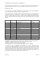
Name of logical operator
Equal to
Not equal to
Greater than
Greater than or equal to
Less than
Less than or equal to
Fortran 77
.EQ.
.NE.
.GT.
.GE.
.LT.
.LE.
Fortran 95
==
/=
>
>=
<
<=
In FORTRAN 95, the continuation marker & must be on the line to be continued, rather than at
the sixth position of the continued line:
Fortran 77:
CL=THETA(6)*GENDER+
xTHETA(7)**AGE
Fortran 95:
CL=THETA(6)*GENDER+
THETA(7)**AGE
&
This affects verbatim code and user-written subroutines. For example, an NMVI version of
CCONTR would be written as follows:
SUBROUTINE CCONTR (I,CNT,P1,P2,IER1,IER2)
PARAMETER (LTH=40,LVR=30,NO=50)
COMMON /ROCM0/ THETA (LTH)
COMMON /ROCM4/ Y
DOUBLE PRECISION CNT,P1,P2,THETA,Y,W,ONE,TWO
DIMENSION P1(*),P2(LVR,*)
DATA ONE,TWO/1.0D+00,2.D+00/
IF (I.LE.1) RETURN
W=Y
Y=(Y**THETA(3)-ONE)/THETA(3)
CALL CELS (CNT,P1,P2,IER1,IER2)
Y=W
CNT=CNT-TWO*(THETA(3)-ONE)*LOG(Y)
RETURN
END
nm730.doc
20 of 210
NONMEM Users Guide: Introduction to NONMEM 7.3.0
Whereas in NM7, it would be written as:
SUBROUTINE CCONTR(I,CNT,P1,P2,IER1,IER2)
USE SIZES, ONLY: ISIZE,DPSIZE
USE ROCM_REAL,
ONLY: THETA=>THETAC,Y=>DV_ITM2
USE NM_INTERFACE,ONLY: CELS
IMPLICIT NONE
INTEGER(KIND=ISIZE), INTENT(IN OUT) :: I,IER1,IER2
REAL(KIND=DPSIZE),
INTENT(IN OUT) :: CNT,P1(:),P2(:,:)
REAL(KIND=DPSIZE) :: ONE,TWO,W
DATA ONE,TWO/1.00D+00,2.00D+00/
SAVE
IF (I.LE.1) RETURN
W=Y(1)
Y(1)=(Y(1)**THETA(3)-ONE)/THETA(3)
CALL CELS (CNT,P1,P2,IER1,IER2)
Y(1)=W
CNT=CNT-TWO*(THETA(3)-ONE)*LOG(Y(1))
RETURN
END
Continuation indicator is allowed in abbreviated code (non-verbatim) lines (NM73)
In NONMEM 7.3.0, extra long lines may be continued using an & at the end of the line:
CL=EXP(THETA(1)*WERT &
+EPS(1))
The total number of characters in the resulting concatenated line may not exceed FSD (default
set to 67000 in sizes.f90). In fact, the continuation marker & may be used on record lines as
well. If the ampersand at the end of a line is not to be interpreted as a continuation marker, but
as a part of the record, then, place a ; after it. For example,
FORMAT=s1PE15.8:160& ;
Alternative Inputs for $OMEGA and $SIGMA Values: VARIANCE/ CORRELATION/
CHOLESKY (NM72)
In NONMEM 7.2.0, OMEGA and SIGMA elements may be entered in forms other than the
default variance diagonal elements and covariance off-diagonal elements. Diagonal elements
may also be entered as standard deviation, and off-diagonal elements may be entered as
correlation values. Options are
VARIANCE/STANDARD to indicate form of diagonal elements
COVARIANCE/CORRELATION to indicate form of off-diagonal elements
CHOLESKY for inputting blocks of OMEGAS or SIGMAS in their Cholesky form.
Examples:
$OMEGA BLOCK(2) ; or $OMEGA VARIANCE COVARIANCE BLOCK(2)
0.64
-0.2402 0.58
$OMEGA STANDARD BLOCK(2)
nm730.doc
21 of 210
NONMEM Users Guide: Introduction to NONMEM 7.3.0
0.8
-0.24 0.762
$OMEGA STANDARD CORRELATION BLOCK(2)
0.8
-0.394 0.762
$OMEGA VARIANCE CORRELATION BLOCK(2)
0.64
-0.394 0.58
$OMEGA CHOLESKY BLOCK(2)
0.8
-0.3 0.7
$SIGMA 0.3 STANDARD 0.8 STANDARD 0.3 VARIANCE
These input options do not affect how estimated OMEGAs and SIGMAs are outputted.
With NONMEM 7.3.0, there are new features for abbreviated code and the $ABBR record.
Each is discussed in greater detail in the on-line help and Guide VIII:
Repeated SAME BLOCK for $OMEGA and $SIGMA Records (NM73)
No need to repeat multiple SAME block segments:
$OMEGA BLOCK(2) SAME(3)
Is equivalent to
$OMEGA BLOCK(2) SAME
$OMEGA BLOCK(2) SAME
$OMEGA BLOCK(2) SAME
The SAME(m) feature is also available for $SIGMA.
$SIGMA BLOCK(2) SAME(3)
Repeated Value Inputs for $THETA, $OMEGA, and $SIGMA (NM73)
As of NM73, repeated inputs of $THETA be entered as follows:
Long-hand:
$THETA 2 2 2 2 (0.001,0.1,1000) (0.001,0.1,1000) (0.001,0.1,1000)
(0.5 FIXED) (0.5 FIXED)
Short-hand:
$THETA (2)x4 (0.001,0.1,1000)x3 (0.5 FIXED)x2
Where xn means to replicate n times. The item to be repeated must always be in parentheses,
and the xn must always be immediately after the item, not before it (4x(0.2) is not permitted).
Repeated inputs of $OMEGA or $SIGMA may be entered as follows:
$OMEGA BLOCK(6)
0.1
0.01 0.1
(0.01)x2 0.1
(0.01)x3 0.1
(0.01)x4 0.1
(0.01)x5 0.1
nm730.doc
22 of 210
NONMEM Users Guide: Introduction to NONMEM 7.3.0
The VALUES(diag,odiag) feature allows one to set up initial values with diagonals diag and offdiagonals odiag. The above example could have been entered as
$OMEGA BLOCK(6) VALUES(0.1,0.01)
For fixed block (such as for omega priors):
$OMEGA BLOCK(6) FIX VALUES(0.15,0.0)
$ABBR DECLARE feature for abbreviated code (NM73)
Integers and arrays may be declared and used in abbreviated code:
$ABBR DECLARE DOSE(100),DOSETIME(100)
$ABBR DECLARE INTEGER I
$ABBR REPLACE feature for abbreviated code (NM73)
Any character string may be replaced. In particular, this allows for symbolic labeling to thetas,
etas, and epsilons. As an example, subscripts to THETAS and ETAS can be given symbolic
names:
$ABBR REPLACE THETA(CL)=THETA(4)
$ABBR REPLACE ETA(CL)=ETA(5)
CL=THETA(CL)*EXP(ETA(CL))
Replacement with selection by data item and parameter is permitted:
$ABBR REPLACE THETA(OCC)=THETA(4,7,10)
$PK
KA=THETA(OCC)
which is equivalent to
$PK
IF (OCC==1) KA=THETA(4)
IF (OCC==2) KA=THETA(7)
IF (OCC==3) KA=THETA(10)
Another Example:
$ABBR REPLACE THETA(SID_KA)=THETA(4,6)
$ABBR REPLACE THETA(SID_CL)=THETA(5,7)
$PK
KA=THETA(SID_KA)
CL=THETA(SID_CL)
which is equivalent to
$PK
IF (SID==1)
IF (SID==2)
IF (SID==1)
IF (SID==2)
KA=THETA(4)
KA=THETA(6)
CL=THETA(5)
CL=THETA(7)
A list of numbers may be given as:
$ABBR REPLACE THETA(SID_KA)=THETA(4,7,10,13)
or by the short-hand
$ABBR REPLACE THETA(SID_KA)=THETA(,4 to 13 by 3)
nm730.doc
23 of 210
NONMEM Users Guide: Introduction to NONMEM 7.3.0
At least one comma must appear, so NMTRAN knows it is a number list, not a variable name.
Another example:
Long-hand:
$ABBR REPLACE THETA(SID_KA)=THETA(4,7,10,13,25,29,33,37)
Short-hand:
$ABBR REPLACE THETA(SID_KA)=THETA(,4 to 13 by 3,25 to 37 by 4)
Easier Inter-occasion variability modeling (NM73)
Abbreviated code Replacement Feature and Repeated Feature of $OMEGA may be combined for
easier Inter-occasion variability modeling. For example,
$ABBR REPLACE ETA(OCC_CL)=ETA(4,7,10)
;when OCC=1, eta(4) to be used: when OCC=2, eta(7) to be used, etc.
$ABBR REPLACE ETA(OCC_V) =ETA(5,8,11)
$ABBR REPLACE ETA(OCC_KA)=ETA(6,9,12)
$PK
CL=TVCL*EXP(ETA(1)+ETA(OCC_CL))
V =TVV *EXP(ETA(2)+ETA(OCC_V))
KA=TVKA*EXP(ETA(3)+ETA(OCC_KA))
$OMEGA BLOCK(3) 0.1 0.01 0.1 0.01 0.01 0.1
$OMEGA BLOCK(3) 0.03 0.001 0.03 0.001 0.001 0.03
$OMEGA BLOCK(3) SAME(2); Repeat OMEGA BLOCK(3) SAME twice
In the above example, the NMTRAN parses the variable name OCC_CL at the underscore, and
determines that there is a data item called OCC with which to associate the variable with the etas
listed.
DO WHILE enhancement (NM73)
DOWHILE may now be used in all blocks of abbreviated code. If a variable is used as a
DOWHILE loop variable, it must be declared:
$ABBR DECLARE DOWHILE I
Recursive random variables ("dowhile recursive variables") may be computed in DOWHILE
blocks, as well as in ordinary abbreviated code. A new example (..\examples\sumdosetn.ctl) uses
DOWHILE for dose super-imposition in a transit compartment, and includes the following:
...
$abbr declare dosetime(100),dose(100)
$abbr declare dowhile i
$abbr declare dowhile ndose
$PK
CALLFL=-2
IF (NEWIND < 2) NDOSE=0
IF (AMT > 0 .and. cmt==1) THEN
NDOSE=NDOSE+1
dosetime(NDOSE)=TIME
DOSE(NDOSE)=AMT
ENDIF
...
$DES
INPT=0
nm730.doc
24 of 210
NONMEM Users Guide: Introduction to NONMEM 7.3.0
I=1
DOWHILE (I<=NDOSE)
IPT=0
IF (T>=dosetime(I)) IPT=DOSE(I)*(T-dosetime(I))**NN*EXP(-KTR*(T-dosetime(I)))
INPT=INPT+IPT
I=I+1
ENDDO
See also ssaddl.ctl, ssonedose.ctl, and ssmultidose.ctl for additional examples.
Subscripted Variables Enhancement (NM73)
Subscripts may be used with user-defined variables that are declared to be arrays using the
$ABBR DECLARE record, and also with certain reserved variables such as THETA. Subscripts
may be integer variables and expressions. For example,
$ABBR DECLARE INTEGER IND
$ABBR DECLARE X(10)
$PK
IND=1
X(IND)=THETA(IND+1)
Autocorrelation (CORRL2) (NM73)
Correlation of residual variables using CORRL2 may now be written in abbreviated code.
For example ( ..\examples\ar1mod.ctl):
$ABBR DECLARE T(NO)
$ABBR DECLARE DOWHILE J
$ABBR DECLARE INTEGER I
…
$ERROR
IF(NEWIND.NE.2)I=0
IF(MDV.EQ.0)THEN
I=I+1
T(I)=TIME
J=1
DOWHILE (J<=I)
CORRL2(J,1)=EXP(-THETA(4)*(TIME-T(J)))
J=J+1
ENDDO
ENDIF
Simulation with autocorrelation is
(..\examples\ar1newsim.ctl).
also
possible.
A
new example is
provided
MOD Function (NM73)
The Fortran intrinsic function MOD may now be used in abbreviated code:
k=MOD(i,j)
MOD returns the remainder when i is divided by j. The variables i and j must be either both
integer or both real. However, this function should not be involved in evaluation of the objective
function.
nm730.doc
25 of 210
NONMEM Users Guide: Introduction to NONMEM 7.3.0
MIN,MAX Functions (NM73)
The Fortran intrinsic functions MIN and MAX may now be used in abbreviated code:
DVALUE=MAX(VAL1,VAL2,VAL3…)
However, this function should not be involved in evaluation of the objective function. IF THEN
statements should be used for those, for example:
DVALUE=VAL1
IF(VAL2>DVALUE) DVALUE=VAL2
IF(VAL3>DVALUE) DVALUE=VAL3
GAMLN Function (NM73)
The GAMLN function returns an accurate evaluation of the logarithm of the gamma function. It
can be used in the evaluation the factorial:
FAC=exp(gamln(x+1.0))
Where
FAC=X!=X*(X-1)*(X-2)…*1
It is more accurate that the Stirling’s approximation, and may be used in abbreviated code in the
evaluation of the objective function.
Declaring Reserved Variables (NM73)
Some useful reserved variables are explicitly recognized by NMTRAN that can be used by the
user. There are however many other variables that are generally internal to NONMEM, and
often are not needed by users except occasionally, which are not explicitly recognized by
NMTRAN, and so cannot be used in abbreviated code, but must be used with verbatim code (“ at
beginning of line). For example the variable ITER_REPORT is available that contains the
present iteration number as reported to the console or NONMEM report file, that may be useful
to be accessed within the $PK, $ERROR, or $PRED code. A convenient means of accessing this
variable, as well as letting NMTRAN allow you to use that variable in abbreviated code is to
place its MODULE definition in an include file that begins with the name
NONMEM_RESERVED (case insensitive) at the beginning of the section you want to use it.
For example, NONMEM_RESERVED_GENERAL in the ..\util directory has many quite useful
variables listed, including ITER_REPORT, in the form of:
"C ITER_REPORT: Iteration number that is reported to output
"C (can be negative, if during a burn period).
"C BAYES_EXTRA, BAYES_EXTRA_REQUEST, used in example 8
" USE NMBAYES_REAL, ONLY: OBJI
" USE NMBAYES_INT, ONLY: ITER_REPORT,BAYES_EXTRA_REQUEST,BAYES_EXTRA
" USE PNM_CONFIG, ONLY: PNM_NODE_NUMBER
“ USE NM_INTERFACE, ONLY: TFI,TFD
The user may use any one of these variables, such as shown in example 8:
$PK
include nonmem_reserved_general
BAYES_EXTRA_REQUEST=1
MU_1=THETA(1)
MU_2=THETA(2)
MU_3=THETA(3)
MU_4=THETA(4)
CL=DEXP(MU_1+ETA(1))
nm730.doc
26 of 210
NONMEM Users Guide: Introduction to NONMEM 7.3.0
V1=DEXP(MU_2+ETA(2))
Q=DEXP(MU_3+ETA(3))
V2=DEXP(MU_4+ETA(4))
S1=V1
IF(BAYES_EXTRA==1 .AND. ITER_REPORT>=0 .AND. TIME==0.0) THEN
WRITE(50,*) ITER_REPORT,ID,CL,V1,Q,V2
ENDIF
Note the lack of needing to begin a line with “ when using ITER_REPORT,
BAYES_EXTRA_REQUEST, or BAYES_EXTRA, because NMTRAN “read” the
nonmem_reserved_general file, and listed the variables declared in there as acceptable to use. A
copy of the nonmem_reserved_general file is in the ..\util directory. It needs to be placed in the
present run directory so NMTRAN has access to it. You could opt to copy only part of the list
in nonmem_reserved_general according to need into any file with name starting with
nonmem_reserved…
A list of useful variables and their meanings are listed in ..\guides\useful_variables.pdf. Be
careful in its use, as you have the ability to change the values of these reserved variables, and this
could crash the system if you change the wrong thing.
Note also that the nonmem_reserved_general file may contain function declarations, such as TFI
and TFD, which are convenient functions to easily convert an integer to text (“text from integer”
TFI) or double precision value to text (“text from double” TFD) . This is quite useful so that the
compiler can catch a misuse of that function’s arguments.
If you wish to define your own function, and have the information about its proper use of
arguments be conveyed upon its execution, so the compiler may detect errors, then one method is
to package the definition of the function in a USE module, such as is done in the following
example:
Myfuncmodule.f90 defines the functions mymin and mymax:
MODULE MYFUNCS
contains
function mymin(a,b,c,d,e)
integer mymin
integer a,b,c,d,e
mymin=min(a,b,c,d,e)
end function
function mymax(a,b,c,d,e)
integer mymax
integer a,b,c,d,e
mymax=max(a,b,c,d,e)
end function
END MODULE MYFUNCS
Nonmem_reserved_myfunc is the include file that declares its use:
" USE myfuncs, only: mymin,mymax
and the following control stream file uses the function:
nm730.doc
27 of 210
NONMEM Users Guide: Introduction to NONMEM 7.3.0
$PROB THEOPHYLLINE
POPULATION DATA
$INPUT
ID DOSE=AMT TIME CP=DV WT
$DATA
THEOPP
$SUBROUTINES
ADVAN2 OTHER=myfuncmodule
$PK
;THETA(1)=MEAN ABSORPTION RATE CONSTANT (1/HR)
;THETA(2)=MEAN ELIMINATION RATE CONSTANT (1/HR)
;THETA(3)=SLOPE OF CLEARANCE VS WEIGHT RELATIONSHIP (LITERS/HR/KG)
;SCALING PARAMETER=VOLUME/WT SINCE DOSE IS WEIGHT-ADJUSTED
include "nonmem_reserved_myfunc"
CALLFL=1
KA=THETA(1)+ETA(1)
K=THETA(2)+ETA(2)
CL=THETA(3)*WT+ETA(3)
SC=CL/K/WT
I=mymin(1,2,3,4,5.0)
print *,'I ',I
$THETA (.1,3,5) (.008,.08,.5) (.004,.04,.9)
$OMEGA BLOCK(3) 6 .005 .0002 .3 .006 .4
$ERROR
Y=F+EPS(1)
$SIGMA
.4
If you use the wrong argument type (real instead of integer), or perhaps use the wrong number of
arguments, the compiler will readily flag this.
Numerical Equality Comparison for IGNORE option in $DATA Record (NM73)
When the IGNORE option is used to filter records from the input file, the .EQ., =, .NE., and /=
symbols perform literal string comparisons. To provide a numerical equality comparison, use
.EQN. for numerical equals, and .NEN. for numerical not equals. For example
$DATA FILE=myfile.txt IGNORE=(OCC.EQN.1)
Will filter out all records for which the data item OCC is equal numerically to 1, even if it is
stored as 1.0, or 1.00e+00, etc.
$DATA FILE=myfile.txt IGNORE=(OCC.EQ.1)
only filters out records for which OCC is literally ‘1’.
I.5 Invoking NONMEM
NONMEM 7.3 can be invoked using one of the supplied scripts:
nmfe73.bat for Windows
nmfe73 for Linux/Unix
nm730.doc
28 of 210
NONMEM Users Guide: Introduction to NONMEM 7.3.0
These script files take at least two arguments, the control stream file name, and the main report
file name, such as:
Windows:
nmfe73 mycontrol.ctl myresults.res
Unix:
./nmfe73 mycontrol.ctl myresults.res
The control stream file name is passed to NONMEM as its first argument. Write and print
statements supplied by the user in verbatim code will be routed as follows:
Unit * prints to console
Unit 6 prints to report file
WRITE(*,… or PRINT *,… : to console
WRITE(6,… to report file.
If you wish to reroute all console output to a file, the execution statement could have a
redirection added to it:
Windows:
nmfe73 mycontrol.ctl myresults.res >console.txt
Linux:
./nmfe73 mycontrol.ctl myresults.res >console.txt
To prevent NONMEM from polling the standard input for ctrl key characters (a new feature
described later):
Windows:
nmfe73 mycontrol.ctl myresults.res -background>console.txt
Linux:
./nmfe73 mycontrol.ctl myresults.res -background>console.txt
In Unix/Linux, you can additionally append & to the command to execute it in the background
(you must also use –background option when using &):
./nmfe73 mycontrol.ctl myresults.res –background >& console.txt &
And periodically monitor the rerouted file:
tail –f
console.txt
For the more adventurous user, you may modify the nmfe73 scripts for alternative behaviors.
Additional options are available to make execution of the nmfe73 script more flexible. From the
nmfe73 command line, the user may enter a run directory that is different from the directory in
which the nmfe73 script is launched:
-rundir=c:\my_favorite_dir
Where rundir is the run directory if it is different from the present working directory (you must
make sure all user dependent input files, control stream file, msf files, and data files, are
available in that run directory).
The user may also enter an alternative name for the constructed executable:
nm730.doc
29 of 210
NONMEM Users Guide: Introduction to NONMEM 7.3.0
-nmexec=nonmem2
specifies an alternative executable name, than the default nonmem.exe (windows) or nonmem
(Linux).
To turn off production of the XML output file root.xml, where root is the root name of the
control stream file, use the option –xmloff.
Beginning in NM73, an additional feature of the execution script file is that the path to the
fortran compiler system and MPI system that is appropriate for NONMEM may be retrieved
from a script file that could have the following environment variables defined:
compilerpath
mpibinpath
mpilibpath
mpilibname
Comments in these files are provided for instructions about each of these environment variables.
These paths will be temporarily added to the front of the PATH environment variable, so that the
appropriate compiler or MPI system is called to service NONMEM. In the past, conflicts with
other installed fortran compilers from other applications would prevent the appropriate compiler
from being used for the NONMEM system. This location file method allows NONMEM to be
forced to look in a particular location.
The location file should be called nmloc.bat or nmloc by convention. It may be specified at the
nmfe73 command line by the -locfile option, for example:
nmfe73 myfile.ctl myfile.res -locfile=nmloc.bat
If –locfile is not specified, the nmfe73 script looks in the present working directory for nmloc.bat
(windows) or nmloc (linux). If this file is not found, it looks in the top directory of the
NONMEM installed directory. Thus, the file nmloc.bat (Windows) or nmloc (Linux) in the top
nonmem installed directory serves as the default location file, and may be modified, or used as a
template and placed in the working directory or specified in the –locfile option on the command
line. If a particular environment variable in the above list is not found or is not defined, then
nmfe73 will behave as in earlier versions, and rely on the presently existing PATH for finding
the compiler and MPI system. The nmfe73 script will display a statement as to what path it will
use.
I.6 Dynamic Memory Allocation (NM72)
With NONMEM 7.2.0 and higher versions, the user need no longer specify “big” or “reg” when
using SETUP72 (or SETUP73) to install NONMEM. (The reg/big/same choice is ignored. It is in
effect always “same” and is shown as “same” in all examples. However, some constants in
SIZES are not dynamically allocated, for example, LSTEXT or PNM_MAXNODES. See help
entry for sizes, or see comments regarding the various parameters in resource\SIZES.f90).
NMTRAN sizes each NONMEM executable only as large as it needs to be for the specific
control stream run. NONMEM 7.2.0 has the ability to dynamically size the main arrays in
NONMEM, according to the number of subjects, and number of parameters described in the
nm730.doc
30 of 210
NONMEM Users Guide: Introduction to NONMEM 7.3.0
control stream file, etc. To do this, NMTRAN determines the appropriate sizes for arrays, and
puts this information in a subroutine called FSIZESR in the FSUBS file. NONMEM
dynamically allocates the sizes of arrays at run-time, based on the values in FSIZESR. Although
unnecessary for most problems, the user may over-ride the size that NMTRAN assesses for a
select number of arrays, by including a $SIZES statement as the first non-comment line of the
control stream file. For example:
$SIZES MAXIDS=230 NO=300 LTH=50 LVR=30
The following is an example of FSIZESR information from a run with CONTROL5. All
parameters can be changed with $SIZES (see resource/sizes.f90 for descriptions and default
values), except NTT, NOMEG, NSIGM, PPDT, which are always evaluated properly by
NMTRAN and should not be over-ridden.
LTH
LVR
LVR2
LPAR
LPAR3
NO
MMX
LNP4
LSUPP
LIM7
LWS3
MAXIDS
LIM1
LIM2
LIM3
LIM4
LIM5
LIM6
LIM8
LIM11
LIM13
LIM15
LIM16
MAXRECID
PC
PCT
PIR
PD
PAL
MAXFCN
MAXIC
PG
NPOPMIXMAX
nm730.doc
3
4
0
10
0
0
1
0
1
0
0
12
0
0
0
0
0
0
0
0
0
0
0
0
0
1
1
7
0
0
0
0
0
31 of 210
NONMEM Users Guide: Introduction to NONMEM 7.3.0
MAXOMEG
MAXPTHETA
MAXITER
ISAMPLEMAX
DIMTMP
DIMCNS
DIMNEW
PDT
LADD_MAX
MAXSIDL
NTT
NOMEG
NSIGM
PPDT
3
4
20
0
0
0
0
4
0
0
3
3
1
3
The file FSIZES is also produced that contains the same contents as the FSIZESR routine in
FSUBS. The FSIZES file is produced for easy reading for the user, and is not used by the
NONMEM system. Those parameters with a 0 cannot be determined or are not given by
NMTRAN and will default to the values hard-coded in resource\SIZES.f90. See the file
SIZES.f90 itself, or on-line help entry for sizes, for these values. On occasion, NMTRAN misinterprets the true scope of the run, and NONMEM may stop the run because one of the sizing
parameters was too low. The user should then insert a $SIZES record in the control stream file,
set the offending sizing parameter to the appropriate value, and run the problem again.
SIZES.f90 no longer contains parameters DIMPKS and DIMRHS and DIMRV for NMTRAN.
The arrays sized by these parameters are dynamically allocated to whatever size is necessary for
the abbreviated code in the current control stream. All other arrays for NMTRAN can be
increased in size if necessary with $SIZES.
As of NM73, NMTRAN determines the maximum number of observation records (MDV=0) that
occur in any subject, among all data files used in the entire control stream file. If this value is
greater than the NO value listed in SIZES.f90, it will set NO to this larger size. Thus, users no
longer have to be conscientious of sizing the NO parameter. However, there is no guarantee that
NMTRAN will correctly assess NO for the entire scope of the control stream file for all types of
problems. Should this occur, NONMEM may issue an error, and the user will need to set the NO
value with a $SIZES record.
When PREDPP ($PK, $ERROR, $INFN, etc.) is used, NMTRAN also creates a sizes file called
prsizes.f90. This file contains sizing and other parameters needed by PREDPP.
Some
parameters (PD, LVR which sets the prsizes parameter PE) are the same as in FSIZES and have
the same values. Some (PC, PCT, PIR, PAL, MAXFCN, MAXRECID) are unique to PREDPP
and prsizes.f90. All may be changed with $SIZES. For example, $SIZES MAXFCN=9000000
might be used with General Non-Linear models ADVAN6, ADVAN8, ADVAN9, ADVAN13)
to request more function evaluations than the default value in resource\SIZES.f90, which is
MAXFCN=1000000. As of NM73, PCT and PIR are assessed by NMTRAN and submitted to
NONMEM, if –prdefault is not used.
nm730.doc
32 of 210
NONMEM Users Guide: Introduction to NONMEM 7.3.0
Usually a parameter value needs to be specified in $SIZES when the problem is bigger than what
is specified in sizes.f90. For example, if LTH=40 in sizes.f90, and your problem needs only 35
thetas, then NONMEM executable will be built to size for 35 thetas, and $SIZES was not
needed. If, however, the problem requires 45 thetas, then
$SIZES LTH=45
or greater needs to be specified, and then NONMEM will be set to a size of LTH=45 as well.
For the following parameters LTH, LVR, PD, PC, DIMTMP, MMX, DIMCNS, and/or PDT,
NMTRAN must anticipate a maximum size, because it needs to set up internal arrays that stores
the information it will gather from the control stream file. It will get this maximum size from the
values in sizes.f90, or from the user specifying the required size in $SIZES. If the user does not
specify in $SIZES, then NMTRAN will determine the best size for the problem and construct the
NONMEM executable accordingly. But if the user specifies a size in $SIZES, then this is also
the size by which the NONMEM executable will be constructed.
To anticipate large sizes without needing to specify values in $SIZES, then set LTH, LVR, PD,
PC, DIMTMP, MMX, DIMCNS, and/or PDT in sizes.f90 to the maximum you think you will
ever need. NTMRAN will still create a NONMEN executable that is sized to fit the problem.
Be aware, however, that if parameter values are set too large, NMTRAN may not run, as it uses
sizes.90 to set its array sizes at the beginning, before it knows the actual size of the problem.
As of NM73, as an alternative to modifying sizes.f90 to very large maximum sizes, you can tell
NMTRAN the maximum size that may be needed by specifying a $SIZES parameter as a
negative value. Thus, a user can give NMTRAN permission to deal with all problems that have
data input files that have up to 1000 data items, and up to 150 omegas, and up to 200 thetas, by
the following:
$SIZES PD=-1000 LVR=-150 LTH=-200
but the size of these parameters when the NONMEM executable is constructed will be only what
is needed for the particular problem. In contrast,
$SIZES PD=1000 LVR=150 LTH=200
will result in sizing the NONMEM executable with these values, and won’t make a “tailor fit”.
This would result in a very large executable regardless of the model size. Thus, $SIZES PD=1000 tells NMTRAN that you may need as many as 1000 data items in a data file, whereas
$SIZES PD=1000 tells NMTRAN that you need exactly that size.
With nonmem 7.1.2 and earlier releases, only FSUBS is compiled at run time. With nmfe72
(NONMEM 7.2.0), or nmfe73 (NONMEM 7.3.0) certain of the PREDPP files in the ..\pr
directory are also compiled at run time, with the sizes and values given in prsizes.f90. Thus,
arrays internal to PREDPP are statically allocated. In contrast, the NONMEM source code in
..\nm are precompiled and the main NONMEM arrays are allocated dynamically. PREDPP
source code is not pre-compiled and dynamically allocated due to significant increase in run
times. Many compilers produce a much more elaborate binary code in order to deal with
variables that are dynamically shaped, which occurs with dynamically sized variables that have
nm730.doc
33 of 210
NONMEM Users Guide: Introduction to NONMEM 7.3.0
more than one dimension to them, and this slows down execution considerably with routines that
are accessed very frequently, such as PREDPP routines.
The nmfe73 script file copies the required PREDPP routines from the nonmem ..\pr directory
into a temporary folder (called temp_dir) under the user’s run directory, and compiles the
routines there. The resulting object files are then linked with NONMEM, and the nonmem
executable is created. The compilation of the PREDPP routines may take some time (about 10 to
50 seconds). If you are repeatedly running the same problem, by default the nmfe73 script will
skip the PREDPP recompilation. It does this by testing that all of the PREDPP files listed in the
file LINK.LNK from the previous run are appropriate for the present run, and testing that the
present prsizes.f90 is not different from the present run.
Typically, you can expect that the nmfe73 script will do a PREDPP recompile when any of the
following sizes change LVR,PD, PC, PCT, PIR, PAL, MAXFCN. This could happen if the user
changes the values via $SIZES. Also, NMTRAN will resize LVR if the number of $OMEGA
entries changes, and it will resize PD if the number of data items listed in $DATA changes. Size
changes are all listed in prsizes.f90 in the PREDPP temporary recompile directory. The
PREDPP files selected for linking (listed in LINK.LNK) can change if the $SUBROUTINES
statement, which specifies ADVAN/TRAN, is changed.
You may force PREDPP recompilation, in case the run does not appear to execute properly when
no recompilation occurs, by setting the –prcompile switch:
nmfe73 mycontrol.ctl myresults.res -prcompile
On the other hand, if the nmfe73 script for some reason believes there is a change in the previous
run from the present run, but you are convinced there is not a change, you may force the skipping
of the PREDPP compilation step and use the compiled files from the previous run by adding the
argument –prsame, at the end of the command line. For example,
nmfe73 mycontrol.ctl myresults.res -prsame
If you are repeatedly going between two or more problems, so that often they need to be
PREDPP recompiled, and you want to save time, you can specify a unique temporary directory
for the PREDPP compilation for a given problem, by using –runpdir option at the nmfe73
command line. For example,
You may run problem A as
nmfe73 mycontrolA.ctl myresults.res -runpdir=mycontrolA
and then follow with problem B as
nmfe73 mycontrolB.ctl myresults.res -runpdir=mycontrolB
When you return to rerunning problem A at some later time:
nm730.doc
34 of 210
NONMEM Users Guide: Introduction to NONMEM 7.3.0
nmfe73 mycontrolA.ctl myresults.res -runpdir=mycontrolA
it won’t need to recompile (assuming your PREDPP sizings and PREDPP model did not change
for problem A), as its PREDPP recompile directory was not overwritten by the intervening call
to problem B.
Finally, if you feel that it is sufficient to use default sizes in sizes.f90 for the various PREDPP
parameters, and therefore use the precompiled routines in ..\pr of the NONMEM installed
directory, you may use the –prdefault option:
nmfe73 mycontrol.ctl myresults.res –prdefault
As of nm73, you may also use the –tprdefault option , which tests if –prdefault is acceptable, and
if so, will use it, otherwise, it will perform a PREDPP recompile:
nmfe73 mycontrol.ctl myresults.res –tprdefault
If you enter
nmfe73 mycontrol.ctl myresults.res –tprdefault –prcompile
then if –prdefault is not acceptable, and will act on the –prcompile option.
If you enter
nmfe73 mycontrol.ctl myresults.res –tprdefault –prsame
then if –prdefault is not acceptable, and will act on the –prsame option.
You may skip the NMTRAN step using the –trskip switch:
nmfe73 mycontrol.ctl myresults.res –background -trskip
The –trskip option is useful if you wish to modify FSUBS created by a previous run, and insert
extra debug lines into FSUBS, and prevent your modified FSUBS from being over-written by
NMTRAN (it will still be compiled). The trskip and any one of prsame, prcompile, or prdefault
switches may be used together.
I.7 Changing the Size of NONMEM Buffers
The entire data set is not necessarily stored in memory at one time. It may be stored in a
temporary disk file, and parts of it are brought into a memory buffer as needed. Some other large
arrays are also stored on disk files. Of course, memory-file swapping of data set information
leads to increased computer run-time. So the bigger the buffer size, the shorter may be the run
time. The sizes of the NONMEM buffers are set by constants LIM1 to LIM16. The default
settings of these constants are set in SIZES.f90. If these constants are not adequate, NONMEM
will produce error messages such as the following.
TOT NO. OF DATA RECS IN BUFFER 1 IS LESS THAN
NO. OF DATA RECS IN INDIVIDUAL REC NO. 1 (IN INDIVIDUAL REC ORDERING)
Unlike most of the other dynamically changeable parameters, NMTRAN does not determine the
most appropriate LIM value for the problem, but instructs NONMEM to use the default value
specified in resource\SIZES.f90 by default. For many problems, the default LIM values are high
enough that all of the data may reside in memory without resorting to the buffer files. For large
nm730.doc
35 of 210
NONMEM Users Guide: Introduction to NONMEM 7.3.0
data sets, buffer files are likely to be used. The user may, however, select a LIM value that is
different from that specified in sizes.f90, via the $SIZES record in the control stream file, e.g.:
$SIZES LIM1=20000
It is not necessary to recompile NONMEM, just rerun the nmfe73 script, and the appropriate
arrays will be allocated according to the user specified LIM value.
It is most desirable to set the LIM value that is the proper size for the run, so that the buffer file
does not have to be used. With today’s very large memory computers, this should usually be
alright to do without running out of memory. Below is a table describing the minimal allowable
value for each LIM, and the value needed to prevent using the buffer file for a particular
problem:
LIM
Minimum
Maximum Value needed to prevent
Buffer files used
Value
buffer file usage
(FILExx)
1
MAXDREC
TOTDREC
10,13,20,33
2
MAXDREC
TOTDREC
39,14
3
2
MAXIDS
12
4
2
MAXIDS
15,16
5
2
MAXIDS
17,18
6
MAXDREC
TOTDREC
7,19
7
2
MAXDREC
21,22
8
2
MAXIDS
23,24
9
NOT USED
10
NOT USED
11
2
NPROB
31,32
12
NOT USED
13
2
MAXIDS
11
14
NOT USED
15
2
MAXIDS
26,27
16
MAXDREC
TOTDREC
26,27
MAXIDS=Largest total number of individual records (subjects) in a data set used in the run
MAXDREC= Largest number of data records in any one individual record (in any one subject)
TOTDREC=total number of data records (lines) in largest data set to be used.
NPROB=Total number of problems in the control stream.
LVR=Largest number of etas in any problem (including those listed in $PRIOR)
As of NM73, the values for MAXDREC and TOTDREC are assessed by NMTRAN, and the
user may take advantage of NMTRAN’s evaluation by using the –maxlim option to the nmfe73
script (see below). But NMTRAN may not always correctly assess these values. Thus, it is best
if the user ascertains these values ahead of time by inspection of his largest data set among all of
the problems to be used by the control stream file, and the largest number of parameters to be
used. Then set the LIM values accordingly via the $SIZES record.
nm730.doc
36 of 210
NONMEM Users Guide: Introduction to NONMEM 7.3.0
One can alternatively assess empirically whether file buffers are used, by beginning the run,
allowing perhaps one iteration to transpire, then from another command window do a directory
search for FILE*, (or WK* for worker files in parallelization problems, section I.53 Parallel
Computing (NM72)). If any of the FILExx do not have 0 size, then they are being used.
Interrupt the analysis, then increase the appropriate LIM value with the $SIZES record, delete
the FILE* in case some remain due to a ctrl-C interrupt, rerun the problem, and look again for
any non-zero sized FILE* again. Repeat as needed.
By default (-maxlim=0), NMTRAN will set the LIM values to those listed in sizes.f90, or to the
minimum required, whichever is larger. As of NM73, if you set –maxlim=1 on the command
line, then LIM1, LIM3, LIM4, LIM13, and LIM15 (those used during estimation, and therefore
by workers in a parallelization problem), will be set to the size needed to assure no buffer files
are used, and everything is stored in memory, for the particular prolem. If you set –maxlim=2,
then LIM1, LIM2, LIM3, LIM4, LIM5, LIM6, LIM7, LIM8, LIM11, LIM13, LIM15, and
LIM16 are also sized to what is needed to assure that buffer files are not needed.
If you set -maxlim=3, then MAXRECID will also be sized, to MAXDREC, the largest number
of records in any individual. MAXRECID sizes arrays involved in storing state variables during
partial derivative estimates of sigmas and sigma like thetas, to improve efficiency of the EM and
Monte Carlo methods. When setting -maxlim=3, it is preferred to also use –tprdefault, or –
prcompile, but not –prdefault, as NMTRAN’s optional resizing of the PREDPP size parameter
MAXRECID may conflict with the –prdefault option.
To specify only a subset of LIM’s to be sized by NMTRAN, set –maxlim to a number list
enclosed within parantheses, such as –maxlim=(1,2,3,11-16), which will have NMTRAN find
size requirements for LIM1, LIM2, LIM3, LIM11, LIM13, LIM15, and LIM16 (LIM12 and
LIM14 are not used). Enclosing the option in quotes “–maxlim=(1,2,3,11-16)” is required for
some operating systems. For sizing MAXRECID, use the number 17. Setting maxlim=(1-17) is
equivalent to –maxlim=3, whereas –maxlim=(3) means to have NMTRAN size only LIM3.
Description of Buffers
A number of contiguous data records are stored in memory at any one time in buffers. If a large
enough memory area can be made available for this purpose, then the entire data set can be
stored in memory throughout the NONMEM run, and computing costs can be decreased. The
following discussion of NONMEM buffers should not be confused with I/O buffers which are
used by the operating system.
The size of buffer 1 is related to the number, LIM1, of data records stored in memory at any one
time. A large proportion of data sets will consist of no more than 10000 data records.
Consequently, the size of buffer 1 has been set to allow LIM1=10000 data records. The least
number of data records allowable must exceed the largest number of data records used with any
one subject, which rarely will be as large as 10000. Each data record consists of PD 8 byte
double precision computer words, and the allocation of memory for buffer 1 is PD*(LIM1+3)*8
bytes.
nm730.doc
37 of 210
NONMEM Users Guide: Introduction to NONMEM 7.3.0
Buffer 2 holds a number of contiguous residual records. For each data record, NONMEM
generates prediction, residual and weighted residual data items, NPDE, EWRES, etc.; these data
items comprise the residual record. The default size of buffer 2 is related to the number, LIM2,
of residual records, stored in memory at any one time. The size of buffer 2 has been set to allow
LIM2=100,000 residual records, for up to 100,000 data records. The least number of residual
records allowable must exceed the largest number of data records used with any one subject.
Each residual data record consists of 19 eight byte double precision computer words. The
allocation of memory for buffer 2 is 19*(LIM2+3)*8 bytes.
Buffer 3 holds a number of contiguous subject header records for input data. The size of buffer
3 is related to the number, LIM3, of subject header records stored in memory at any one time.
The default size of buffer 3 has been set to allow LIM3=1000 subject header records. Each
subject header record consists of four 8 byte computer words. The allocation of memory for
buffer 3 is 4*(LIM3+1)*8 bytes.
Buffer 4 holds a number of contiguous ETA records. For each subject, NONMEM generates
values for ETA variables. The size of buffer 4 is related to the number, LIM4, of ETA records
stored in memory at any one time. The size of buffer 4 has been set to allow LIM4=1000 ETA
records. Each ETA record consists of MMX*LVR 8 byte double precision computer words. The
allocation of memory for buffer 4 is MMX*LVR*(LIM4+3)*8.
Buffer 5 holds a number of contiguous mixture model records. For each subject record,
NONMEM generates information about the component models of a mixture model; this
information constitutes the mixture model record. The size of buffer 5 is related to the number,
LIM5, of mixture model records stored in memory at any one time. The default size of buffer 5
has been set to allow LIM5=200 mixture model records. Each mixture model record consists of
five 8 byte single precision computer words. The allocation of memory for buffer 5 is
(MMX+1)*(LIM5+3)*8 bytes.
Buffer 6 holds a number of contiguous PRED-defined records. For each data record of a given
subject record, NONMEM stores the values found in module NMPRD4; these values comprise
the NMPRD4 record. The size of buffer 6 is related to the number, LIM6, of PRED-defined
records stored in memory at any one time. The size of buffer 6 has been set to allow LIM6=400
PRED-defined records. The least number of PRED-defined records allowable must exceed the
largest number of data records used with any one subject, which rarely will be as large as 400.
Each PRED-defined record consists of PDT 8 byte double precision computer words. The
allocation of memory for buffer 6 is PDT*(LIM6+3)*8 bytes.
Buffer 7 holds a number of contiguous NMPRD4 records for a single individual only. For each
problem in a NONMEM run, NONMEM generates information about the problem; this
constitutes the problem header record. The size of buffer 7 is related to the number, LIM7, of
NMPRD4 records stored in memory at any one time. The size of buffer 7 has been set to allow
LIM7=2 NMPRD4 records, which is generally fewer than the number of NMPRD4 records
existing for any given subject. Each NMPRD4 record consists of (LIM7+2)*LNP4 8 byte double
precision computer words. The default allocation of memory for buffer 7 is 4*LNP4*8 bytes.
nm730.doc
38 of 210
NONMEM Users Guide: Introduction to NONMEM 7.3.0
The memory allocation of Buffer 8 is (LVR+1)*(LIM8+3) double precision values.
Buffer 11 holds a number of contiguous problem header records. The size of buffer 11 is related
to the number, LIM11, of problem header records stored in memory at any one time. The size of
buffer 11 has been set to allow LIM11=25 problem header records. Each problem header record
consists of forty-two 8 byte integer computer words. The allocation of memory for buffer 11 is
42*(LIM11+3)*8= 9408 bytes.
The memory allocation of Buffer 13 is 404*(LIM13+3) double precision values.
After NONMEM VI, there are also buffers 15 and 16. The sizes of these buffers are related
to constants LIM15 and LIM16. These buffers are used in DAT15 and DAT16. If
LIM16 is , not adequate, NONMEM will produce error messages such as the following.
TOT NO. OF RESIDUAL RECS IN BUFFER 16 IS LESS THAN
NO. OF DATA RECS WITH SOME INDIVIDUAL
The memory allocation of Buffer 15 is LCM110*(LIM15+3) double precision values.
The memory allocation of Buffer 16 is MMX*4*(LIM16+3) double precision values.
Buffers 1, 3, 4, 13, and 15 are used during an estimation step. To obtain the fastest analysis,
even when the estimation is parallelized, you may want to optimize their LIM sizes.
I.8 Multiple Runs
As of NONMEM 7, there is decreased likelihood of early termination of runs using multiple
problems and/or the “Super Problem” feature.
I.9 Improvements in Control Stream File input limits
1. By default, there may be up to 50 data items per data record. In NM72, set PD in $SIZES
record to change this.
2. Data labels may be up to 20 characters long
3. Numerical values in the data file may now be up to 24 characters long.
4. ID values in the data file may be up to 14 digits long.
5. The numerical values in $THETA, $OMEGA, and $SIGMA may be each up to 30 characters
long, and may be described in E field notation.
6) By default, you may have up to 50 items printed in tables. In NM72, set PDT in $SIZES
record to change this.
I.10 Issuing Multiple Estimations within a Single Problem
A sequence of two or more $EST statements within a given problem will result in the sequential
execution of separate estimations. This behavior differs from NONMEM VI, where two
sequential $EST statements acts as the continuation of defining additional options to a single
estimation. For example:
nm730.doc
39 of 210
NONMEM Users Guide: Introduction to NONMEM 7.3.0
$THETA 0.3 0.5 6.0
$OMEGA 0.2 0.2 0.2
$SIGMA 0.2
; First estimation step
$EST METHOD=0 MAXEVAL=9999
PRINT=5 NSIG=3
; Second estimation step
$EST METHOD=CONDTIONAL
NSIG=4
will first result in estimation of the problem by the first order method, using as initial parameters
those defined by the $THETA, $OMEGA, and $SIGMA statements. Next, the first order
conditional estimation method will be implemented, using as initial parameters the final
estimates of THETA, OMEGA, and SIGMA from the previous analysis. Up to 20 estimations
may be performed within a problem. For all intermediate estimation steps, their final parameter
values and objective function will be printed to the raw output file.
Many settings to options specified in a $EST method will by default carry over to the next $EST
method, unless a new option setting is specified. Thus, in the example above, PRINT will
remain 5 and MAXEVAL will remain 9999 for the second $EST statement, whereas NSIG will
be changed to 4 and METHOD becomes conditional. An exception to this rule are
NOTHETABOUND, NOOMEGABOUND, and NOSIGMABOUND, in which these options
pertain to all of the estimations in the series within a $PROB. In NM710, NM712, and NM720,
these options must be given with the very first $EST record in the problem. With NM73, these
options may be placed with any of the $EST records, but will still apply to all $EST records in
the problem.
The EM and Monte Carlo estimation methods particularly benefit from performing them in
sequence for a given problem. Even the classical NONMEM methods can be facilitated using an
EM method by first having a rapid EM method such as iterative two stage be performed first,
with the resulting parameters being passed on to the FOCE method, to speed up the analysis:
$EST METHOD=ITS INTERACTION
$EST METHOD=CONDITIONAL INTERACTION
More information on this is described in the Composite Methods section.
I.11 Interactive Control of a NONMEM batch Program
A NONMEM run can now be controlled to some extent from the console by issuing certain
control characters.
Console iteration printing on/off during any Estimation analysis (ctrl-J from console NONMEM,
Iterations button from PDx-POP).
Exit analysis at any time, which completes its output, and goes on to next mode or estimation
method (ctrl-K from console, or Next button in PDx-POP).
Exit program gracefully at any time (ctrl-E or Stop button).
nm730.doc
40 of 210
NONMEM Users Guide: Introduction to NONMEM 7.3.0
Monitor the progress of each individual during an estimation by toggling ctrl-T. Wait 15
seconds or more to observe a subject’s ID, and individual objective function value. It is also
good to test that the problem did not hang if a console output had not been observed for a long
while.
If you run NONMEM from PDx-POP, you can get graphical view of objective function or any
model parameter progress during the run. The parameter and objective function progress is
written in a root.ext file (where root is base name of control stream file), which may also be
monitored by a text editor during the run.
If you run NONMEM from PDx-POP, Bayesian sample histories of the population parameters
can be viewed after analysis is done. The sample history file is written to that specified by the
$EST FILE= option, which can be also monitored by a text editor during or after the run.
Sometimes NONMEM does not respond to user input. This may occur during a parallel
distribution run using MPI, or if the user began NONMEM with the –background switch. The
user may open another console window, copy the program sig.exe from the NONMEM installed
..\util directory to your run directory, then enter any one of these commands:
Print toggle (monitor estimation progress):
Sig J
Sig R
Sig P
Paraprint toggle (monitor parallel processing traffic):
Sig B
Sig A
Sig PA
Sig PP
Next (move on to next estimation mode or next estimation):
sig K
sig N
Stop (end the present run cleanly):
Sig E
Sig S
Subject print toggle:
sig T
sig U
sig SU
Alternatively, you may execute the sig program from another directory if you specify the run
directory in which you want the signal file created:
nm730.doc
41 of 210
NONMEM Users Guide: Introduction to NONMEM 7.3.0
sig next \nonmem\run\
Make sure you terminate the directory name with a directory parse symbol appropriate for the
operating system.
I.12 $COV: Unconditional Evaluation
The covariance step can be performed unconditionally even when an estimation terminates
abnormally, by specifying:
$COV UNCONDITIONAL
I.13 $TABLE: Additional Statistical Diagnostics, Associated Parameters, and
Output Format
Requesting a Range of Etas to be Outputted: Etas(x:y) (NM73)
Instead of requesting each ETA specifically in a $TABLE item list, a range of etas may be
requested:
ETAS(2:4)
is equivalent to requesting ETA2, ETA3, and ETA4.
ETAS(5)
or
ETAS(5:LAST)
is equivalent to requesting ETA(5), ETA(6), … to ETA(NETAS).
The $SCAT will also interpret this syntax, for example,
$SCAT ETAS(1:2) VS ETA3
is equivalent to
$SCAT ETA1 ETA2 VS ETA3
However, unlike $TABLE, $SCAT will ignore implied endings, such as
$SCAT ETAS(1:LAST) VS ETA3
And just interpret it as
$SCAT ETA1 VS ETA3
New diagnostic items
Additional types of pred, res, and wres values may be requested than the usual set available in
NONMEM VI. They may be specified at any $TABLE command or $SCATTER command, as
one would request PRED, RES, or WRES items. If $TABLE statements succeed multiple $EST
nm730.doc
42 of 210
NONMEM Users Guide: Introduction to NONMEM 7.3.0
statements within a run, the table results (as well as scatter plots if requested via $SCATTER)
will pertain to the last analysis.
OBJI
These are objective function values for each individual. The sum of the individual objective
function values is equal to the total objective function.
NPRED, NRES, NWRES
These are non-conditional, no eta-epsilon interaction, pred, res, and wres values. These are
identical to those issued by NONMEM V as PRED, RES, and WRES.
PREDI, RESI, WRESI
These are non-conditional, with eta-epsilon interaction, pred, res, and wres values. These are
identical to those issued by NONMEM VI as PRED, RES, and WRES. The WRESI will not
differ from NWRES if INTERACTION was not selected in the previous $EST command.
CPRED, CRES, CWRES
These are conditional, no eta-epsilon interaction, pred, res, and wres values as described in [1].
The conditional mode etas (from FOCE or ITS, also known as conditional parametric etas (CPE),
empirical bayes estimates (EBE), posthoc estimates of etas, or mode a posteriori (MAP)
estimates) or conditional mean etas (from Monte Carlo EM methods) will be referred to as η̂
(eta hat), must be available from a previous $EST MAXEVAL>0 command. The conditional
weighted residuals are estimated based on a linear Taylor series approximation that is
extrapolated from the conditional mean or mode (or posthoc) eta estimates, rather than about
eta=0:
ˆ   gij (η
ˆ )η
ˆ
CPREDij  fij (η
using the nomenclature of Guide I, Section E2. Then
CRESij  yij  CPREDij
The population variance covariance of observed data described in Guide I, E.2 is also evaluated
at eta_hat: Ci ( ηˆ ) :
ˆ )i1/2 (y i  CPREDi (η
ˆ ))
CWRESi= C(η
Because of the linear back extrapolation, it is possible for some CPRED values to be negative.
Users may prefer to request NPRED CRES CWRES, or NPRED RES CWRES. The conditional
weighted residual will not differ from the non-conditional weighted residual if FO was selected
in the previous $EST command.
In NM72, if $EST INTERACTION was not specified prior to requesting $TABLE CWRES,
then the population variance-covariance is evaluated at eta=0: Ci ( η  0) . In NONMEM 7.1.0
and 7.1.2, regardless of INTERACTION setting in a previous $EST statement, Ci ( ηˆ ) is used.
nm730.doc
43 of 210
NONMEM Users Guide: Introduction to NONMEM 7.3.0
CPREDI, CRESI, CWRESI
These are conditional, with eta-epsilon interaction, pred, res, and wres values. The conditional
mode or conditional mean etas must be available from a previous $EST MAXEVAL>0
command.
EPRED, ERES, EWRES
The EPRED, ERES, EWRES are Monte-Carlo generated (expected, or exact) pred, res, and wres
values, and are not linearized approximations like the other diagnostic types.
The expected diagnostic items are evaluated using predicted function and residual variances
evaluated over a Monte Carlo sampled range of etas with population variance Omega. Define
EPREDij  


fij ( η p( η   Ωdη
is the expected predicted value for data point j of subject i for a given subject, evaluated by
Monte Carlo sampling, overall possible eta. The probability density of eta:
p(η   Ωdη
is a multivariate normal distribution with eta variance Ω. The 1xni vector of EPRED for a given
subject, where ni is the number of data points to that subject, is then:

EPREDi   fi ( η p( η   Ωdη

Then the corresponding residual vector for observed values yi is
ERESi=yi-EPREDi
The residual (epsilon) variance matrix using the nomenclature in Guide I, Sections E.2 may be
Vi (η  diag (hi (ηΣhi (η))
or it may be the more complicated form described in section of E.4 in the case of L2 data items.
Then, the expected residual (epsilon) variance (assessed by Monte Carlo sampling) is

EVi   Vi ( η p( η | 0, Ωdη

The full variance-covariance matrix of size nixni, that includes residual error (epsilon) and intersubject (eta) variance contributions is:

ECi  EVi   (fi (η)  EPREDi )(fi ( η)  EPREDi ) p( η | 0, Ωdη

And is the expected population variance, Monte Carlo averaged over all possible eta. Then,
following the Guide I, section E nomenclature, the population weighted residual vector for
subject i is:
EWRESi  ECi1/2ERESi
where the square root of a matrix is defined here by default as evaluated by diagonalizing the
matrix, and multiplying its eigenvector matrices by the square roots of the eigenvalues.
Selecting the WRESCHOL option obtains the square root of the matrix by Cholesky
decomposition.
nm730.doc
44 of 210
NONMEM Users Guide: Introduction to NONMEM 7.3.0
ECWRES
ECWRES is a Monte Carlo assessed expected weighted residual evaluated with only the
predicted function evaluated over a Monte Carlo sampled range of etas with population variance
Omega, while residual variance V is always evaluated at conditional mode (from the most recent
FOCE/ITS estimation) or conditional mean (from the most recent IMP/IMPMAP/SAEM
analysis) eta ( η̂ ), so that

ˆ    (fi (η)  EPREDi )(fi ( η)  EPREDi ) p( η | 0, Ωdη
ECCi  Vi (η

and
ECWRESi  ECCi1/2ERESi
As with CWRES, the eta_hat (conditional mode or mean) values must be available from a
previous $EST MAXEVAL>0 command.
Thus, ECWRES is the Monte Carlo version of CWRES, while EWRES is the Monte Carlo
version of CWRESI.
In NM72, if $EST INTERACTION was not specified prior to requesting $TABLE CWRES,
then the residual variance is evaluated at eta=0: Vi ( η  0 . In NONMEM 7.1.0 and 7.1.2,
regardless of INTERACTION setting in a previous $EST statement, Vi ( ηˆ  is used.
NPDE
The NPDE is the normalized prediction distribution error (reference [2]: takes into account
within-subject correlations), also a Monte Carlo assessed diagnostic item. For each simulated
vector of data yki:
ESRESki=yki-EPREDi
its decorrelated residual vector is calculated:
ESWRESki  ECi1/2ESRESki
and compared against the decorrelated residual vector of observed values EWRESi such that
1 K
  EWRESi  ESWRESki )
K k 1
For K random samples, where
  x)  1 for x  0
 0 for x  0
For each element in the vector. Then, an inverse normal distribution transformation is
performed:
pdei 
npdei  1 (pdei )
nm730.doc
45 of 210
NONMEM Users Guide: Introduction to NONMEM 7.3.0
NPD
The NPD is the correlated normalized prediction distribution error (reference [3]: does not take
into account within-subject correlations), also a Monte Carlo assessed diagnostic item. For each
simulated vector of data yki:
IWRESki= V(ηk )i1/2 (y ki  fi (ηk )
These are then averaged over all the random samples;
1 K
pdi   (IWRES ki )
K k 1
Then, an inverse normal distribution transformation is performed:
npdi  1 (pdi )
The default PRED, RES, and WRES will be given the same values as PREDI, RESI, and
WRESI, when INTERACTION in $EST is specified, or NPRED, NRES, and NWRES when
INTERACTION in $EST is not specified.
As the PRED, RES, and WRES, may be referenced in a user-supplied $INFN routine, or in $PK
or $PRED (when ICALL=3) as PRED_, RES_, WRES_, so the additional parameters may be
referenced by their names followed by _ (for example EWRES_).
CIWRES, CIPRED,CIRES, CIWRESI (NM73)
The CIWRES is the conditional individual weighted residual as evaluated during the estimation,
equivalent to (DV-F)/(F*SQRT(SIGMA(1,1))) for simple problems with proportional residual
error. With L2 data or CORRL2 data, the individual weighted residuals are in their decorrelated
forms:
ˆ )i1/2 (y i  fi ( η
ˆ ))
CIWRESi= V(η
when INTERACTION in the previous $EST record is set, and a conditional analysis (non-FO)
was performed. For individual i, where individual residual variance matrix Vi and individual
predicted vector fi ( ηˆ ) are evaluated at the conditional mode or mean eta (designated as eta hat).
The square root of the matrix Vi may be evaluated by using the square root of the eigenvalues, or
by Cholesky decomposition when WRESCHOL option is used (see below). Similarly, the
CIPRED is the individual predicted value fi ( ηˆ ) at the conditional mode or mean eta, and
CIRES=DV- fi ( ηˆ ) .
When INTERACTION is not set, then
ˆ ))
CIWRESi= V(η  0)i1/2 (y i  fi ( η
is evaluated, that is, the variance portion is evaluated using fi ( η  0) . However CIWRESI
(conditional individual weighted residual with interaction) is always evaluated as (except for FO,
see below)
ˆ )i1/2 (y i  fi ( η
ˆ ))
CIWRESIi= V(η
regardless of the INTERACTION setting.
nm730.doc
46 of 210
NONMEM Users Guide: Introduction to NONMEM 7.3.0
For FO, the conditional individual weighted residual will not differ from the non-conditional
weighted residual. That is, for FO, the CIWRES and CIPRED are evaluated using F(eta=0) for
numerator and denominator terms, since this is what is done during estimation, and no EBE (etahat) is evaluated:
CIWRESi= V(η  0)i1/2 (yi  fi (η  0)) =CIWRESIi
Even for FO with interaction, the predicted function (numerator) and residual variance
(denominator) is still evaluated at eta=0, so CIWRESI=CIWRES. The interaction contribution
is accounted for with additional first-order Taylor terms to make a linear projection of the
contribution of eta-eps interaction. While it would be inappropriate to add these Taylor terms to
CIWRESI, these Taylor terms are added to the population residual assessment WRESI, hence
WRESI will differ from NWRESI with FO INTERACTION.
There are other individual residual values available, mostly as place holders in the system, but
these have no additional statistical value. They are:
NIPRED=IPREDI=NPRED=IPRD
CIPREDI=CIPRED
EIPRED=EPRED
NIRES=IRESI=NRES=IRS
CIRESI=CIRES
EIRES=ERES
NIWRESi= V(η  0)i1/2 (yi  fi (η  0))
IWRESI=NIWRES=IWRS

EIWRESi=  V( η)i1/2 (y i  fi ( η)) p( η | 0, Ωdη

MDVRES=0 (NM73) (default)
Set MDVRES to 1 in the $ERROR or $PRED routine if you do not want to include a particular
value for weighted residual assessment. This may be useful when, for example, this data point is
assessed by a non-normal distribution likelihood such as the PHI() function for below detection
limit values, in which F_FLAG is set. By default, if at least one data value of a given subject is
fitted with a non-normal distribution likelihood, then population weighted residual diagnostics
are not assessed for any of the data for that subject. By setting MDVRES=1 to these particular
below detection values, the weighted residual algorithm can assess the remaining normally
distributed values for that subject. For example,
$ERROR
SD = THETA(5)
IPRED = LOG(F)
DUM = (LOQ - IPRED) / SD
CUMD = PHI(DUM)
IF (TYPE .EQ. 1) THEN
F_FLAG = 0
nm730.doc
47 of 210
NONMEM Users Guide: Introduction to NONMEM 7.3.0
Y = IPRED + SD * ERR(1)
ENDIF
IF (TYPE .EQ. 2) THEN
F_FLAG = 1
Y = CUMD
MDVRES=1
ENDIF
MDVRES stands for missing data value (MDV) for residual (RES) assessment. Setting
MDVRES to 1 is equivalent to temporarily declaring that data point as missing during the
weighted residual assessments.
To incorporate LOQ data into NPDE assessments [4], use the following method (as an example):
Here, TYPE and LOQ are user-defined in previous code, or data item.
$ERROR
SD = THETA(5)
IPRED = LOG(F)
DUM = (LOQ - IPRED) / SD
CUMD = PHI(DUM)
IF (TYPE .EQ. 1.OR.NPDE_MODE.EQ.1) THEN
F_FLAG = 0
Y = IPRED + SD * ERR(1)
ENDIF
IF (TYPE .EQ. 2.AND.NPDE_MODE.EQ.0) THEN
F_FLAG = 1
Y = CUMD
MDVRES=1
ENDIF
IF(TYPE.EQ.2) DV_LOQ=LOQ
By default, DV_LOQ is set to -1.0d-300 by the NONMEM routine that calls ERROR/PRED. If
the user’s ERROR/PRED sets DV_LOQ to some other value and NPDE_MODE=1, then the
NPDE is being evaluated during that time, and this censored value is to be treated as if it is a
non-censored datum with value of LOQ (DV_LOQ=LOQ), in accordance with [4], utilizing a
standard F_FLAG=0 definition for Y. Note that during estimation of the objective function
(when NPDE_MODE=0), NPDE is not being evaluated, and censored values should be treated
using F_FLAG=1, and Y must be defined as the integral of the normal density from –inf to LOQ.
ESAMPLE=300
Number of random samples to be used to generate a Monte-Carlo based set of EPRED, ERES,
ECWRES, NPDE, and EWRES. ESAMPLE should be specified only on the first $TABLE
command. By default, ESAMPLE=300.
WRESCHOL (NM73)
Normally, population and individual weighted residuals are evaluated by square root of the
eigenvalues of the population or individual residual variance. However, an alternative method is
to Cholesky decompose the residual variance (suggested by France Mentre, personal
nm730.doc
48 of 210
NONMEM Users Guide: Introduction to NONMEM 7.3.0
communication), by entering the WRESCHOL option. This should be specified only on the first
$TABLE command. The Cholesky form has the property of sequentially decorrelating each
additional data point in the order of the data set.
SEED
Specify starting seed for Monte Carlo evaluations of EPRED, ERES, EWRES, ECWRES, and
NPDE. The default seed is 11456. SEED should be specified only on the first $TABLE
command.
RANMETHOD=[n|S|m|P] (NM72) (default n=3)
By default, the random number generator used for Monte Carlo simulations of weighted residual
items is ran3 of reference [5]. We feel this is the best random number generator for many
purposes. However, you may choose alternative random number generators as follows:
0: ran0 of reference [5], minimal standard generator
1: ran1 of reference [5], Bays and Durham.
2: ran2 of reference [5].
3: ran3 of reference [5], Knuth.
4: NONMEM’s traditional random number generator used in $SIMULATION
RANMETHOD should be specified only on the first $TABLE command. The RANMETHOD
set in the $TABLE command does not propagate to $EST or $CHAIN.
As of NM73, the Sobol sequences with scrambling may be requested:
RANMETHOD=[n|S|m|P]
where n is the random number generator type, S is Sobol sequence, and m is the Sobol
scrambler, and P may be specified to retain separate seed patterns for each subject, so that the
random pattern is retained regardless of single or parallel processing. See the description of
RANMETHOD under I.25 Monte Carlo Importance Sampling EM.
Among the Sobol sequence methods, the S2 method appears to provide the least biased random
samples, that is nearly uniform distribution, with good mixing in multi-dimensional spaces.
NOLABEL (NM73)
Do not print column labels. It may be combined with ONEHEADER to print only the title at the
beginning of each table.
NOTITLE (NM73)
Do not print table titles. It may be combined with ONEHEADER to print only the column labels
at the beginning of each table. NOLABEL NOTITLE is equivalent to NOHEADER.
nm730.doc
49 of 210
NONMEM Users Guide: Introduction to NONMEM 7.3.0
FORMAT=,1PG13.6
This parameter defines the delimiter and number format for the present table, and subsequent
tables, until a new FORMAT is specified. The first character defines the delimiter, which may
be s for space, t for tab, or the comma. The default format is
s1PE11.4
The syntax for the number format is Fortran based, as follows:
For E field:
xPEw.d
indicates w total characters to be occupied by the number (including decimal point, sign, digits,
E specifier, and 2 digit magnitude), d digits to the right of the decimal point, and x digits to the
left of the decimal point.
Examples:
E12.5: -0.12345E+02
2PE13.6: -12.12345E+02
If you are outputting numbers that are less than 1.0E-99, such as 1.22345E-102, there will be one
less significant digit displayed to make room for the extra digit in the exponent. To make room
for a three digit exponent, you may set the format as follows:
xPEw.dEe
where e is the number of digits to be provided for the exponent. For example
1PE12.4E3: -2.3456E+002
For F field:
Fw.d
indicates w total characters to be occupied by the number (including decimal point, sign and
digits), d digits to the right of the decimal point.
Examples:
F10.3: -0.012, 234567.123
For G field:
xPGw.d
For numbers >=0.1, will print an F field number if the value fits into w places showing d digits,
otherwise will resort to xPEw.d format. For numbers <0.1, will always use xPEw.d format.
If the user-defined format is inappropriate for a particular number, then the default format will be
used for that number.
An example $TABLE record could be:
nm730.doc
50 of 210
NONMEM Users Guide: Introduction to NONMEM 7.3.0
$TABLE ID CMT EVID TIME NPRED NRES PREDI RESI WRESI CPRED CRES CWRES CPREDI
CRESI CWRESI=ZABF EPRED ERES EWRES PRED RES WRES NPDE=PDERR ECWRES
NOPRINT NOAPPEND FILE=myfile.tab ESAMPLE=1000 SEED=1233344
LFORMAT, RFORMAT (NM72)
An alternative format description to FORMAT is RFORMAT and LFORMAT. RFORMAT
(where R=real numbers) describes the full numeric record of a table, so that formats for specific
columns may be specified. LFORMAT (where L=label) specifies the format of the full label
record of a table. The formats must be enclosed in double quotes, and (), and have valid Fortran
format specifiers. The RFORMAT and LFORMAT options can be repeated if the format
specification is longer than 80 characters. Multiple RFORMAT and LFORMAT entries will be
concatenated to form a single format record specification. For example,
LFORMAT="(4X,A4,4(',',4X,A8))"
RFORMAT="(F8.0,"
RFORMAT="4(',',1PE12.5))"
Will result in the following formats submitted to a Fortran write statement:
LFORMAT=(4X,A4,4(',',4X,A8))
for the table’s label record, and
RFORMAT=(F8.0,4(',',1PE12.5))
For the table’s numeric records. If RFORMAT and LFORMAT are given, then the FORMAT
option will be ignored. By default, FORMAT, RFORMAT, LFORMAT specifications will be
passed on to the next $TABLE record in a given problem unless new ones are given. To turn
off an RFORMAT/LFORMAT specification in a subsequent table (and therefore use FORMAT
instead), set
LFORMAT="NONE"
RFORMAT="NONE"
Here is an example of $TABLE statements designated in a control stream file:
$TABLE ID TIME PRED RES WRES CPRED CWRES EPRED ERES EWRES NOAPPEND ONEHEADER
FILE=tabstuff.TAB NOPRINT,FORMAT=,1PE15.8
$TABLE ID CL V1 Q V2 FIRSTONLY NOAPPEND NOPRINT FILE=tabstuff.PAR
LFORMAT="(4X,A4,4(',',4X,A8))"
RFORMAT="(F8.0,"
RFORMAT="4(',',1PE12.5))"
$TABLE ID ETA1 ETA2 ETA3 ETA4 FIRSTONLY NOAPPEND NOPRINT
FILE=tabstuff.ETA,FORMAT=";F12.4"
LFORMAT="NONE"
RFORMAT="NONE"
There is no NMTRAN error checking on the RFORMAT and LFORMAT records, so the user
must engage in trial and error to obtain a satisfactory table output (you should set MAXEVAL=0
or MAXEVAL=1 for the $EST step to do a quick check, so you don’t spend hours on estimation
only to find the RFORMAT/LFORMAT were not appropriate).
nm730.doc
51 of 210
NONMEM Users Guide: Introduction to NONMEM 7.3.0
A word of caution. The FORMAT descriptor 1P, which means move the decimal point to the
left by 1, will be in effect for all remaining FORMAT components. For example, in
RFORMAT="(F8.0,37(',',1PE13.6),24(',',F7.2))"
the F field format that follows an E field format, in which 1P was used, will also have the
decimal placed to the left, and a 1.00 would appear as a 10.00. To prevent this from occurring,
revert to no decimal shift with 0P:
RFORMAT="(F8.0,37(',',1PE13.6),24(',',0PF7.2))"
I.14 $SUBROUTINES: New Differential Equation Solving Method
As of NM7, A differential equation solver has been introduced, called LSODA, and is accessed
using ADVAN=13 or ADVAN13. This routine is useful for stiff and non-stiff equations. This is
similar to the LSODI routine used by ADVAN9, except that ADVAN13 can at times execute
more quickly than ADVAN9. The ADVAN 13 differential equation solver has been shown to
solve problems more quickly with the new estimation methods, whereas for classical NONMEM
methods, selecting ADVAN 6 or 9 may still be of greater advantage.
Example:
$SUBROUTINES ADVAN13 TRANS1 TOL=5
Where TOL is the number of digits accuracy desired to integrate the differential equations
(accuracy to within 10-TOL). The code to the differential equation solver is found in
..\source\LSODA.f90. On occasion, coded errors will be displayed if the algorithm is having
trouble integrating the equations. These errors may usually be ignored, unless the error shows up
frequently, and ultimately results in failure for the problem to complete. Typically the remedy is
to increase or decrease TOL, but for those who desire to understand what the error codes mean,
there are well documented comments on these at the beginning of LSODA.f90. They are printed
here for convenience:
! ISTATE=An index used for input and output to specify the the state of the calculation.
!
!
On input,the values of istate are as follows.
!
1 Means this is the first call for the problem (initializations will be done).
!
See note below.
!
2 Means this is not the first call,and the calculation is to continue
!
normally, with no change in any input parameters except possibly TOUT
!
and ITASK. (If ITOL,RTOL,and/or ATOL are changed between calls with
!
ISTATE=2,the new values will be used but not tested for legality.)
!
3 Means this is not the first call,and the calculation is to continue
!
normally,but with a change in input parameters other than TOUT and ITASK.
!
changes are allowed in NEQ,ITOL,RTOL,ATOL,IOPT,LRW,LIW,JT,ML,MU and any
!
optional inputs except H0,MXORDN,AND MXORDS.
!
(see IWORK description for ML and MU.)
!
Note: A preliminary call with TOUT=T is not counted as a first call here,as
!
no initialization or checking of input is done. (Such a call is sometimes
!
useful for the purpose of outputting the initial conditions.) Thus the first
!
call for which TOUT /= T requires ISTATE=1 on input.
!
!
On output,istate has the following values and meanings.
!
1 Means nothing was done; TOUT=T and ISTATE=1 on input.
!
2 Means the integration was performed successfully.
!
-1 Means an excessive amount of work (more than MXSTEP steps) was done on
nm730.doc
52 of 210
NONMEM Users Guide: Introduction to NONMEM 7.3.0
!
!
!
!
!
!
!
!
!
!
!
!
!
!
!
!
!
!
!
!
!
!
!
!
!
!
!
!
!
!
!
!
!
!
!
-2
-3
-4
-5
-6
-7
this call,before completing the requested task,but the integration was
otherwise successful as far as T. (MXSTEP is an optional input and is
normally 500.) TO continue,the user may simply reset ISTATE to a value > 1
and call again (the excess work step counter will be reset to 0).
In addition,the user may increase MXSTEP to avoid this error return
(see below on optional inputs).
Means too much accuracy was requested for the precision of the machine
being used. This was detected before completing the requested task,but
the integration was successful as far as T. To continue,the tolerance
parameters must be reset,and ISTATE must be set to 3. The optional output
TOLSF may be used for this purpose. (Note: If this condition is detected
before taking any steps,then an illegal input return (ISTATE=-3) occurs
instead.)
Means illegal input was detected,before taking any integration steps.
See written message for details.
Note: If the solver detects an infinite loop of calls to the solver with
illegal input,it will cause the run to stop.
Means there were repeated error test failures on one attempted step,before
completing the requested task,but the integration was successful as far as T.
The problem may have a singularity,or the input may be inappropriate.
Means there were repeated convergence test failures on one attempted step,
before completing the requested task,but the integration was successful as
far as T. This may be caused by an inaccurate jacobian matrix, if one is
being used.
Means EWT(I) became zero for some I during the integration. Pure relative
error control (ATOL(I)=0.0) was requested on a variable which has now
vanished. The integration was successful as far as T.
Means the length of RWORK and/or IWORK was too small to proceed,but the
integration was successful as far as T. This happens when DLSODA chooses
to switch methods but LRW and/or LIw is too small for the new method.
Note: Since the normal output value of ISTATE is 2, it does not need to be
reset for normal continuation. Also,since a negative input value of ISTATE
will be regarded as illegal, a negative output value requires the user to
change it, and possibly other inputs,before calling the solver again.
ATOL (NM72)
An option when using ADVAN13 is the absolute tolerance. The ATOL for ADVAN13 by
default is 12 (that is, precision is 10-12). Usually the problem runs quickly when using
ADVAN13 with this setting. On occasion, however, you may want to reduce ATOL (usually set
it equal to that of TOL), and improve speeds of up to 3 to 4 fold. ATOL may be set at the $EST
or $COV command. The absolute tolerance is set to the same ATOL for all compartments.
As of NM73, ATOL also acts on ADVAN9’s differential equation solver, where by default
absolute significant digits accuracy (absolute tolerance) is 12.
The relative tolerance for ADVAN13 is still set by TOL by the $SUBROUTINES, $COV, or
$TOL record, just as it is for the other differential equation solver ADVAN’s.
MXSTEP (NM73)
Additional control may be obtained by setting the maximum number of integration steps (default
is 10000)
$PK
MXSTEP=5000
ADVAN9’s maximum integration steps can also be controlled by this variable.
nm730.doc
53 of 210
NONMEM Users Guide: Introduction to NONMEM 7.3.0
I.15 $EST: Improvement in Estimation of Classical NONMEM Methods
In pre-NM7 NONMEM installations, the classical first order conditional estimation methods
tended to be particularly sensitive to the formation of a non-positive definite Hessian matrix
during the estimate of etas. In NONMEM 7, if the user selects NOABORT as a $EST option,
most Hessian matrices will be forced to be positive definite if not already, allowing the program
to continue, and abnormal termination of an estimation will occur less often. The occasional
occurrence and correction of non-positive definite Hessian matrices during the intermediate steps
does not typically result in erroneous results. Even with the NOABORT option, there is one
remaining component in the NONMEM algorithm for which positive definite correction is not
performed, which can still cause problems at the beginning of an estimation. It remains so the
user may diagnose a serious problem in the setup of the estimation. Should this still be a
nuisance, in NONMEM 7.2.0 the user may select the NOHABORT option, which will perform
positive definite correction at all levels of the estimation, but it can hide a serious ill-posed
problem, so use with care.
I.16 Controlling the Accuracy of the Gradient Evaluation and individual objective
function evaluation
In classical NONMEM methods (First order, First order conditional, Laplace), the user specifies
SIGDIGIT or NSIG to indicate the number of significant digits that population parameters are to
be evaluated at the maximum likelihood. If NSIG=3 (the default), then the problem would be
optimized until all of the parameters varied by less than 3 significant digits. This same NSIG
value would also be used to specify relative step size (h) to each THETA, SIGMA, and
OMEGA, for evaluating the partial derivative of the objective function with respect to the
parameter. Such partial derivative evaluations are needed to set up gradients to determine the
direction the search algorithm must travel to approach the minimum of the objective function.
The forward finite difference of the partial derivative of O (the objective function) with theta(1)
would be evaluated as
O(1 (1  h))  O(1 )
1h
Numerical analysis of forward finite difference methods [6] recommends that the ideal relative
step size h for the parameter theta(1) should be no greater than SIGL/2, where SIGL is the
significant digits to which the objective function is evaluated. If h is set to a precision of SIGL/2
(which for the present discussion we mean it is set to 10-SIGL/2), then the resulting derivative itself
will have approximately SIGL/2 precision as well.
In the main search algorithm, finite central difference methods are also used. These are
evaluated as:
O(1 (1  h))  O(1 (1  h))
21h
Numerical analysis of central finite difference methods recommend that the ideal relative step
size h for the parameter theta(1) should be no greater than SIGL/3. If h is set to SIGL/3, then the
resulting finite difference value itself will have approximately 2*SIGL/3 precision.
nm730.doc
54 of 210
NONMEM Users Guide: Introduction to NONMEM 7.3.0
The main search algorithm also utilizes pseudo-second derivative type evaluations using forward
difference methods. For these calculations, an ideal h would be 10-SIGL/3, resulting in precision of
second derivative constructs of about SIGL/3. Thus, it is safest to set the step size h, as specified
by NSIG, to be no more than SIGL/3.
An internal SIGL in NONMEM specifies the precision to which the objective function itself
(actually, the individual subject objective functions, which sum to the total objective function) is
to be evaluated. This internal SIGL is set to 10. As long as NSIG was set to a value less then or
equal to 10/2 or 10/3, then the gradients would be evaluated to an appropriate precision to make
the gradient search algorithm work efficiently. With many subjects, if SIGL=10 is the precision
to which each individual objective function is evaluated, and they are all of the same sign, then
the sum objective function could have a resulting precision of log10(N)+SIGL, where N is the
number of subjects, for a maximum of 15, the limiting precision of double precision. Thus with
100 subjects, the actual precision that the total objective function is evaluated could be 12. One
should not necessarily rely on this, so it is safest to suppose the more conservative precision of
10, for which a suitable NSIG would be 3.
For analytical problems, those which do not utilize $DES, one can usually expect a reasonably
efficient convergence to the minimum of the objective function with NSIG=3. However, with
differential equation problems (those used for ADVAN 6, 8, 9, or the new ADVAN method, 13),
the limiting precision that objective function values may be evaluated is not based on the internal
SIGL of 10, but rather, on the TOL level set by the user (where TOL represents the relative
significant digits precision to which differential equations are to be integrated, so the precision is
10-TOL), which is used by PREDPP when differential equations are integrated. The relationship
between the predicted value and the individual subject’s maximized objective function is
complex, but one can use the rule of thumb that the individual’s objective function is evaluated
to a precision of the smaller of TOL and the internal SIGL. Thus, when a user specifies a
TOL=4, then it may well be that the sum objective function has no greater precision than 4. If
the user then specifies NSIG=3, then the main search algorithm evaluates finite gradients using
step size h that varies theta at the 3rd significant digit. This results in 1 significant digit precision
remaining in evaluating the finite difference gradients. The search algorithm is now attempting
to maximize the objective function to 3 significant digits, when it is working with gradients that
are accurate to only 1-2 significant digits. This results in inefficient advancement of the
objective function, causing NONMEM to make repeated evaluations within an iteration, as well
as iterations for which the objective function is barely moving. NONMEM can then spend many
hours trying to obtain precision in its parameters which are impossible to obtain. Eventually it
may stop because the maximum iterations were used up, or when it realizes that it could not
reach the desired precision.
With this understanding of the search algorithm process, and recognizing the complex
relationship between the step size needed for each parameter and the finite difference method
used in each part of the algorithm, the optimization algorithm was changed to allow the user to
specify SIGL, and for the algorithm to set up the appropriate step size for a given finite
difference method, based on the user-supplied SIGL. While some trial and error may still be
required by the user for a given problem, certain general rules may be considered.
nm730.doc
55 of 210
NONMEM Users Guide: Introduction to NONMEM 7.3.0
1) Set SIGL, NSIG, and TOL such that:
SIGL<=TOL
NSIG<=SIGL/3
With these options, the algorithm sets up the following:
For forward finite difference, h is set to SIGL/2 precision
For central finite difference, h is set to SIGL/3 precision
For forward second order difference, h is set to SIGL/3 precision
The individual fits for evaluating optimal eta values will be maximized to a precision of the usersupplied SIGL value
Optimization of population parameters occurs until none of the parameters change by more than
NSIG significant digits.
For the $COV step, the step size for evaluating the R matrix (central difference second
derivative) is set to SIGL/4, which according to numerical analysis, yields the optimal precision
of SIGL/2 for the second derivative terms. If only the S matrix is evaluated (central difference
first derivative), then the step size for it is set to SIGL/3. (But see $COV: Additional Options
and Behavior for a way to set SIGL and TOL for $COV, distinct from the option for the $EST
command).
If the user sets NSIG>SIGL/3, and specifies SIGL, then the optimization algorithm will do the
following, which is a less than optimal setup:
For forward finite difference, h is set to NSIG precision
For central finite difference, h is set to NSIG precision
For forward second order difference, h is set to NSIG precision
The individual fits for evaluating optimal eta values will be maximized to a precision of the usersupplied SIGL value
Optimization of population parameters occurs until none of the parameters change by more than
NSIG significant digits.
For the $COV step, the step size for evaluating the R matrix (central difference second
derivative) is set to SIGL/4, which according to numerical analysis, yields the optimal precision
of SIGL/2 for the second derivative terms. If only the S matrix is evaluated (central difference
first derivative), then the step size for it is set to SIGL/3.
If the user does not specify SIGL, or sets SIGL=100, then the optimization algorithm will
perform the traditional NONMEM VI optimization, which as discussed above, may not be ideal:
For forward finite difference, h is set to NSIG precision
For central finite difference, h is set to NSIG precision
For forward second order difference, h is set to NSIG precision
The individual fits for evaluating optimal eta values will be maximized to a precision of
SIGL=10
nm730.doc
56 of 210
NONMEM Users Guide: Introduction to NONMEM 7.3.0
Optimization of population parameters occurs until none of the parameters change by more than
NSIG significant digits.
For the $COV step, the step size for evaluating the R and S matrix is set to NSIG, as is done in
NONMEM VI. This is far from optimal, particularly for analyses requiring numerical
integration, and is often the cause of the inability to evaluate the R matrix.
Command syntax:
Example:
$EST METHOD=1 INTERACTION SIGL=9 NSIG=3
To see the advantage of properly setting NSIG, TOL , and SIGL, consider the following
problem, which is example 6 at the end of this document. Data were simulated with 17 PK and
18 PD observations for each of 50 subjects receiving a bolus of drug, followed by short infusion
a week later. The PK model has 2 compartments (Vc, k12, k21) with first-order (k10) and
receptor-mediated clearance (Vmax, Kmc). The PD model is indirect response, with receptors
generated by zero order process (k03), and removed by first order process (k30) or via drugreceptor complex (Vmax, Kmc). There are 46 population parameters, variances/covariances, and
intra-subject error coefficients, and thee differential equations. In the table below are listed the
estimation times (not including a $COV step) using various SIGL, NSIG, and TOL values. Note
that when not setting SIGL (NM 6 method), the problem would take a very long time. When
SIGL, NSIG, and TOL were set properly, estimation times were much less, with successful
completions. Of course, as they say in the weight-loss commercials, individual results may
vary, and such great differences in execution times will not occur for all problems.
Advan method
NSIG=3
NSIG=2
TOL=6
TOL=6
SIGL=100 (NM6 style) SIGL=6
NSIG=1
TOL=4
SIGL=3
9 >30
22
10
6 >24
17
3
13 (new) >20
8.5
2
I.17 The SIGLO level (NM72)
As of NONMEM 7.2.0, the user may obtain even greater control of the precision at which
various parts of the estimation are performed by using the SIGLO option. If used, the SIGLO
option is the precision to which the individual etas are estimated. The SIGL level set by the user
continues to be the precision (or delta ) setting for the finite difference algorithms in the higher
level estimation process for THETAS, OMEGAS, and SIGMAS. By default, if SIGLO is not
specified, then SIGLO is set to the same value as SIGL, and everything is evaluated in
accordance with the previous paragraph. Should SIGLO be used, the recommended setting
would be:
nm730.doc
57 of 210
NONMEM Users Guide: Introduction to NONMEM 7.3.0
SIGLO<=TOL
SIGL<=SIGLO
NSIG<=SIGL/3
I.18 Alternative convergence criterion for FO/FOCE/Laplace (NM72)
Sometimes many iterations will occur with very little change in the objective function, even with
SIGL/TOL adjustment. This may occur because a parameter may oscillate at the 2nd significant
digit, for example, and NSIG was set to 3. The parameter may never settle down to a value that
fluctuates at less than NSIG significant digits if its contribution to the objective function is very
small. Thus, a minimum objective function is achieved, but NONMEM’s traditional
convergence test, based on all parameters changing by less then NSIG significant digits, is never
satisfied. An alternative convergence test is to set CTYPE=4 in the $EST statement. NONMEM
will then additionally test if the objective function has not changed by more then NSIG digits
beyond the decimal point over 10 iterations. If this condition is satisfied, the estimation will
terminate successfully.
I.19 Additional Control for $MSFI record (NM73)
Sometimes the MSFI error check is too strict, and prevents an MSF file from being utilized in a
subsequent control stream file or problem. This occurs particularly when using classical
NONMEM methods. To turn off MSFI error checking, set NOMSFTEST (default is
MSFTEST):
$MSFI myfilename NOMSFTEST
I.20 Options for $ESTIMATION Record for alternative MAP (eta optimization)
methods and evaluating individual variances by numerical derivative methods for
FOCE/Laplace (NM73).
OPTMAP=0 (default) (NM73)
0: Standard variable metric (Broyden, Fletcher, Goldfarb, and Shanno (BFGS)) optimization
method used by NONMEM to find optimal eta values (aka EBE, CPE, MAP, or conditional
mode estimates, referred to symbolically ˆ , or eta hat) for each subject at the mode of their
posterior densities, using analytical derivatives of F with respect to etas, and analytical
derivatives of H with respect to etas, that were supplied by NMTRAN or by the user.
1: Variable metric method, using numerical finite difference methods for first derivatives of F
with respect to etas. Necessary when not all code used in evaluating F, G and H for observation
event records is abbreviated code (some may be in verbatim code), and/or some portions of the
computation of F, G and H are evaluated in a hidden subroutine specified by "$SUBROUTINES
OTHER=" and the user-written code does not compute the eta derivatives. When OPTMAP=1 is
present, values of G and H are ignored during eta optimization. This may be used to test usercoded derivatives, because two runs, one with OPTMAP=1 and one without it, should give very
similar values for the OBJV, WRES, etc. if the user-coded derivatives are correct. That is, the
nm730.doc
58 of 210
NONMEM Users Guide: Introduction to NONMEM 7.3.0
analytic derivatives in G and H are ignored, and this option may be used when analytic
derivatives are difficult to compute (e.g., user supplied code such as SDE).
2: Nelder Mead method, which uses a secant method, rather than relying on derivatives.
ETADER=0 (default) (NM73)
In evaluating the MAP objective function, the term log(Det(V)) must be evaluated to obtained
the marginal or integrated posterior density, where V is the eta Variance matrix based on the
subject’s posterior density.
0: Expected value V, using analytical first derivatives
1: Expected value V, using forward finite difference numerical first derivatives. Needed if not
all code evaluating F and Y derivatives with respect to eta are available for processing by NMTRAN or in user supplied code.
2: Expected value V, using central finite difference numerical first derivatives. Needed if not all
code evaluating F and Y derivatives with respect to eta are available for processing by NMTRAN or in user supplied code. That is, the analytic derivatives in G and H are ignored, and
this option may be used when analytic derivatives are difficult to compute (e.g., user supplied
code such as SDE).
3: 2nd derivative method of evaluating V, using numerical second derivatives of -log(L) with
respect to etas. This is equivalent to using the “Laplace NUMERICAL method, even though
FOCE may be selected.
When relying on numerical derivatives by using OPTMAP>0 or ETADER>0, you may need to
set the SLOW option for proper estimation of FOCE or Laplace (SLOW is not utilized by
EM/BAYES methods). Note also that non Monte Carlo weighted residual diagnostics (such as
NWRES, NWRESI, CWRES, CWRESI) use first derivatives of F with respect to eta, and the
appropriate numerical derivatives will be used to assess them if ETADER>=1.
NUMDER=0 (default) (NM73)
The file root.fgh is produced if the user selects $EST NUMDER=1.
numerically evaluated derivatives of Y or F with respect to eta, where
G(I,1)=partial F with respect to eta(i))
G(I,J+1)=Second derivatives of F with respect to eta(i),eta(j)
H(I,1)=partial Y with respect to eps(i)
H(i,j+1)=partial Y with respect to eps(i),eta(j))
The file lists the
This option is useful for comparing with and checking analytic derivatives values.
The analytical derivatives values are stored in root.agh, if NUMDER=2 is selected. If you want
both, set NUMDER=3.
MCETA=0 (Default) (NM73)
0: Eta=0 is initial setting for MAP estimation
FOCE/LAPLACE/ITS/IMPMAP, and sometimes IMP.
nm730.doc
(eta
optimization)
during
59 of 210
NONMEM Users Guide: Introduction to NONMEM 7.3.0
1: ETA=values of previous iteration is initial setting for MAP estimation, or ETA=0, whichever
gives lower objective function.
>1: MCETA-1 Random samples of ETA, using normal random distribution with variance
OMEGA, are tested. Plus previous ETA is tested, and ETA=0 is tested. The test is, whichever
supplies the lowest objective function is the eta set used as initial parameters for the MAP
optimization.
NONINFETA=0 (default) (NM73)
NONMEM has traditionally not assessed post-hoc eta hat (also known as empirical Bayes
Estimates, EBE’s, conditional mode etas, or conditional parametric etas (CPE)), if the derivative
of the data likelihood with respect to that eta is zero for a given subject, and simply specified that
eta as zero. This eta is called a non-influential eta. The true EBE is zero anyway, if this eta is not
correlated by an off-diagonal omega element with an eta that is influential. If the non-influential
eta is correlated with an influential eta, then the true EBE of the non-influential eta will in
general not be 0. When NONINFETA=0, the default, then this traditional algorithm is in effect,
so that all non-influential etas, even those correlated with influential etas, will be reported as 0
when outputted with $TABLE. However, if NONINFETA=1, then all etas are involved in the
MAP estimation, regardless of their influence. This will result in non-influential etas reported as
a non-zero value, if it is correlated with influential etas. From a pure statistical stand-point, this
is the true EBE, although intuitively it may be puzzling for some users. Whether
NONINFETA=1 or 0, the individual’s objective function will change very little if at all, because
NONMEM provides a corrective algorithm to assess the correct objective function. But for
purposes of post-hoc evaluated etas, one may wish to set NONINFETA depending on the desired
interpretation. The NONINFETA option applies only to FO/FOCE/Laplace. The Monte Carlo
and EM methods have always used (even with earlier versions of NONMEM 7) the pure
statistical option (NONINFETA=1).
FNLETA=1 (default) (NM72)
Set FNLETA to 0 if you do not want it to spend time performing the end FNLMOD (which
evaluates final mixture proportions for each subject in mixture models) and FNLETA (which
evaluates final etas) routines using the original algorithm after the estimation and covariance
steps are completed. You may want to turn this off if each objective function call takes a long
time, with very complex problems or large data sets. NONMEM will use instead a more
efficient means, which has not been thoroughly vetted. Be aware, that certain $TABLE outputs,
such as the traditional WRES, RESI, and PRED, may or may not be properly evaluated if the
FNLMOD and FNLETA steps are omitted.
Normally, when you do not set FNLETA, or when you set FNLETA to 1, regardless of the
method that was used (classical or EM/Monte Carlo) to obtain the thetas, omegas and sigmas in
the last $EST step, $TABLE parameters are estimated based on a “post-hoc” evaluation of the
etas at the mode of the posterior density position (eta hat). These eta hat values are identical to
those evaluated during the estimation for ITS/FOCE/Laplace methods, but differ from the
conditional mean values estimated during an IMP, SAEM analysis. Setting FNLETA=0
prevents the post-hoc analysis, so that $TABLE parameters are evaluated based on the eta values
generated by the last iteration of the last $EST method implemented, which are mode of
nm730.doc
60 of 210
NONMEM Users Guide: Introduction to NONMEM 7.3.0
posterior values for ITS/FOCE/Laplace, and conditional means for IMP/SAEM. The etas after a
BAYES analysis yields single sample position values of the very last iteration, and have limited
use.
Regardless of the FNLETA setting, the .phi and .phm tables (see I.47 $EST: Additional Output
Files Produced) always output the phi/eta values used for the particular method (mode of
posterior, and approximate Fisher information based variances for ITS/FOCE/Laplace methods,
Monte Carlo assessed conditional means and conditional variances for SAEM/IMP methods).
If you set FNLETA=2 (NM73), then the estimation step is not done, and whatever etas are stored
in memory at the time are used in any subsequent $TABLE’s. This has value if you loaded the
individual etas from an MSF file, or from a $PHIS/$ETAS record, and you want to calculate
$TABLE items based on those etas, rather than from a new estimation. For example:
$PROB
$INPUT C ID GRP AMT TIME DV1 DV CMTS EVID MDV
$DATA mydata.csv IGNORE=C
…
$MSFI=myresults.MSF
…
$EST METHOD=1 FNLETA=2
$TABLE ID TIME DV IPRED CMTS MDV EVID NOAPPEND NOPRINT FILE=mytable.tab
I.21 Bootstrap, Selecting a Random Method, and Other Options for Simulation
(NM73)
BOOTSTRAP (NM73)
$SIML BOOTSTRAP=-1 SUBP=100
$EST METHOD=1 INTERACTION
The above example requests a bootstrap rearrangement (with replacement) of an existing data
set, followed by analysis of that data set. The BOOTSTRAP number refers to how many subjects
are to be randomly selected from the data set. Setting -1 or to a value larger than the number of
subjects in the data set means to randomly select as many subjects as are in the data set. For
example, if 400 subjects are in the simulation template data set, then 400 subjects are randomly
selected (with replacement, so some are selected more than once, others not at all). In this case,
NONMEM’s simulator does not perform the usual activity of randomly creating DV values for a
new data set, but rather selects a random set of subjects of an existing data set (which must
already have legitimate DV values), uniformly selected (using seed1) with replacement. This
results in some subjects not being selected at all, and some subjects selected more than once.
NOREPLACE (NM73)
$SIML BOOTSTRAP=50 SUBP=100 NOREPLACE
$EST METHOD=1 INTERACTION
In the above example, 50 unique subjects are to be randomly selected from the simulation
template data set. The NOREPLACE feature is reasonable if there are many more than 50
subjects to choose from template set (for example, 1000 subjects in the template, and for each
nm730.doc
61 of 210
NONMEM Users Guide: Introduction to NONMEM 7.3.0
sub-problem, 50 of them are randomly chosen without replacement, that is, without repeating a
subject).
STRAT (NM73)
$SIML BOOTSTRAP=50 SUBP=100 NOREPLACE STRAT=CAT
A single stratification data item may be entered. In the above example, the data item CAT serves
as the stratification. This splits the data set into distinct sub-sets, guaranteeing a specific number
of subjects will be selected from each category. For example, if in the base data set CAT has
values of 1 or 2, with 33 subjects in group 1 and 67 subjects in group 2 out of 100 total subjects,
then exactly 33% of of subjects from group 1 will be randomly selected out of 50 total (16), and
exactly 67% of subjects will be randomly selected from group 2 (34). This has value when
desiring that a bootstrap analysis maintain the same proportion of subjects belonging to certain
categories, such as gender, or age bracket. To stratify by both age bracket and gender, create a
stratification data item that would be, for example, valued 1 for subjects who are male under 30,
2 for subjects that are female under 30, 3 for subjects who are male over 30, 4 for subjects who
are female over 30. Any discrete numerical values will do, as long as the stratifier is not a
continuous variable, and the subjects need not be sorted according to the stratification data item.
STRATF (NM73)
$SIML BOOTSTRAP=50 SUBP=100 NOREPLACE STRAT=CAT STRATF=FCAT
The option STRATF points to a data item that contains the fraction that should represent a
category in the bootstrapped data set. Without STRATF, the number of subjects to be taken
from a given category is proportional to the number of subjects in the base data set. If you want
the category to be represented at a different proportion, then specify a STRATF data item, in this
example, FCAT. Suppose FCAT=0.5 for CAT=1 and 0.5 for CAT=2 as well. Even though only
33% of subjects in the base data set belong to category 1, exactly 50% of subjects from group 1
will be randomly selected out of 50 total (25), and exactly 50% of subjects will be randomly
selected from group 2 (25) in the formation of each bootstrap data set. This allows you to alter
the proportions in each category from what is in the original data det.
RANMETHOD=[n|S|m|P] (NM73)
As of NM73, the RANMETHOD option is available for the $SIM record, to use alternative
random numbers generators (default is NONMEM’s traditional one, number 4):
$SIML RANMETHOD=[n|S|m|P]
Where n is the random number generator type, S is Sobol sequence, and m is the Sobol
scrambler. See the description of RANMETHOD under I.25 Monte Carlo Importance
Sampling EM.
NONMEM’s default random number generator for the $SIM step is 4 (in contrast, default
random number generator for $EST and $TABLE is 3). Number 4 is NONMEM’s classic
nm730.doc
62 of 210
NONMEM Users Guide: Introduction to NONMEM 7.3.0
random number generator. Whatever random number generator is selected, it affects all seed1
sources, and all source seed2.
The Sobol method is used only to generate normally distributed random vectors of etas and
epsilons, when the S descriptor is selected, and SEED1 source 1 is used to set the seed. Among
the Sobol sequence methods, the S2 method appears to provide the least biased random samples,
that is nearly uniform distribution, with good mixing in multi-dimensional spaces.
I.22 Some Improvements in Nonparametric Methods (NM73)
EXPAND (NM73)
$NONP EXPAND
After the parametric estimation is performed, the final eta MAP (or empirical Bayes estimates,
EBE) estimates, based on the final SIGMAS, OMEGAS, and THETAS, are normally used as
support points. If the natural distribution of etas among subjects is highly non-normal, with large
tails, or there are several outlier subjects, the final Omega values may constrain the EBE’s of
these outliers so they do not fit these subjects well. When EXPAND is selected, an alternative
set of EBE’s are evaluated using the initial OMEGA values, but using the final THETAS and
SIGMAS. It is recommended that the initial OMEGAs have inflated values relative to the final
OMEGAS (which is usually the case), to allow the outlier subjects to be fitted with little
constraint from the population distribution. For each subject, the EBE that provides the highest
individual likelihood value (not the highest posterior density) , whether from the final fit EBE, or
the expanded OMEGA EBE, is selected as a support point. This is the inflated variance
recommendation from [7].
NPSUPP (NM73)
$NONP NPSUPP=50
Number of total support points to be used. If NPSUPP>number of subjects, then extra support
points are randomly created from the final OMEGAS (even when EXPAND is selected for the
base EBE support points). This is the extended Grid Method as described in [7].
NPSUPPE (NM73)
$NONP NPSUPPE=50
Number of total support points to be used. If NPSUPPE>number of subjects, then extra support
points are randomly created from the initial, presumably inflated, OMEGAS (even when
EXPAND is not selected for the base EBE support points).
BOOTSTRAP (NM73)
$NONP BOOTSTRAP
The original data set is fitted during the parametric estimation ($EST), and the eta support points
from the original data set are used for the nonparametric version. However, a bootstrap sample,
with subjects uniformly randomly selected with replacement from the original data set, is used
for the nonparametric distribution analysis. This is the simplified bootstrap technique described
in [8]. To provide a series of simplified bootstrap analyses, as an example,
nm730.doc
63 of 210
NONMEM Users Guide: Introduction to NONMEM 7.3.0
$SIML (12345) SUBP=100
$EST METHOD=COND INTERACTION MAXEVAL=9999 NSIG=3 SIGL=10 PRINT=5 NOABORT
$NONP BOOTSTRAP EXPAND
In the above example, BOOTSTRAP option is given in $NONP, along with the $SIML
statement, without a BOOTSTRAP option. On the first sub-problem NONMEM will pass the
original data to the estimation step ($EST), to obtain final THETAS, OMEGAS, and SIGMAS,
with EBE’s adjusted for expansion (EXPAND), followed by a nonparametric density analysis on
the original data set. On the second sub-problem, the estimation step is skipped, but the final
THETAS, OMEGAS, SIGMAS, and EBE’s from the first analysis are retained, and a
nonparametric density analysis is performed on a bootstrap version of the original data set.
For a full bootstrap analysis method, as described in [8]:
$SIML (12345) SUBP=100 BOOTSTRAP=-1
$EST METHOD=COND INTERACTION MAXEVAL=9999 NSIG=2 PRINT=5 NOHABORT
$NONP EXPAND NSUPPE=50
In the above example, 100 bootstrap analyses are performed. The $SIML provides a bootstrap
version of the original data set for estimation by $EST, this is followed by EBE assessment on
the original data set, followed by nonparametric density assessment on the bootstrap data set.
STRAT,STRATF (NM73)
As with $SIML, options STRAT and STRATF are available for the $NONP BOOTSTRAP
record to provide stratified selections (see STRAT (NM73) in I.21 Bootstrap, Selecting a
Random Method, and Other Options for Simulation (NM73).
Three files are produced providing nonparametric information:
root.npd
Each row contains information about a support point: The support point number, the ID from
which the support point was obtained as an EBE of that subject (ID is -1 if this support point was
randomly generated because NSUPP/NSUPPE was greater than number of subjects). The eta
values of the support point are listed, followed by the cumulative probability (CUM) associated
with each eta, followed by the joint density probability of that support point, if default or
MARGINALS was selected. If ETAS was selected, then instead of cumulative probabilities, the
support point eta vector that best fits that subject (ETM) is listed.
root.npe
The expected value etas and expected value eta covariances (ETC) are listed for each problem or
sub-problem. Because only one line is written per problem or sub-problem, the column header is
displayed (unless $EST NOLABEL=1) only once for the entire NONMEM run. However, each
line contains information of table number, problem number, sub-problem number, super problem
and iteration number.
root.npi
The individual probabilities are listed in this file. The header line (unless $EST NOLABEL=1)
is written only once, at the beginning of the file, per NONMEM run. Each line contains
information of table number, problem number, sub-problem number, super problem, iteration
nm730.doc
64 of 210
NONMEM Users Guide: Introduction to NONMEM 7.3.0
number, subject number, and ID. This is followed by the individual probabilities at each support
point (of which there are NSUPP/NSUPPE or NIND of them, whichever is greater). The line
with Subject number=0 contains the joint probability of each support point (the same as listed in
root.npd under the column PROBABILITY). For each support point K, the joint probability is
equal to the sum of the individual probabilities over all subject numbers I. Thus row of subject
number I, column of support K, contains the individual probability IPROB(I,K). The sum of the
individual probabilities over all support points for any given line (subject), is equal to 1/NIND.
The format of the file is fixed at (,1PE22.15), and cannot be changed. It is intended for use in
further analysis by analytical software, and is designed to report the full double-precision
information of each probability.
I.23 Introduction to EM and Monte Carlo Methods
Expectation-maximization methods use a two step process to obtain parameters at the maximum
of the likelihood. In the expectation step, the thetas, omegas, and sigmas are fixed, while for
each individual, expected values (conditional means) of the eta’s and their variances are
evaluated. If necessary, expected values of gradients of the likelihood with respect to the thetas
and sigmas are also evaluated, integrated over all possible values of the etas. From these
constructs, the thetas and sigmas are updated during the maximization step using these
conditional means of the etas and/or the gradients. The omegas are updated as the sample
variance of the individual conditional means of the etas, plus the average conditional variances
of the etas. The maximization step is therefore typically a single iteration process, requiring very
little computation time. The more accurately these constructs are evaluated during the
expectation step, the more accurately the total likelihood will be maximized.
I.24 Iterative Two Stage (ITS) Method
Iterative two-stage evaluates the conditional mode (not the mean) and first order (expected) or
second order (Laplace) approximation of the conditional variance of parameters of individuals by
maximizing the posterior density. This integration step is the same as is used in FOCE or
Laplace. Population parameters are updated from subjects’ conditional mode parameters and
their approximate variances by single iteration maximization steps that are very stable (usually
converging in 50-100 iterations). Because of approximations used, population parameters almost,
but not quite, converge towards the linearized objective function of FOCE. Iterative two stage
method is about as fast as FOCE with simple one or two compartment models, and when set up
with MU referencing (described below) can be several fold faster than FOCE with more complex
problems, such as 3 compartment models, and differential equation problems.
The iterative two stage method is specified by
$EST METHOD=ITS INTERACTION NITER=50
where NITER (default 50) sets maximum number of iterations. For all new methods, it is
essential to set INTERACTION if the residual error is heteroscedastic.
nm730.doc
65 of 210
NONMEM Users Guide: Introduction to NONMEM 7.3.0
I.25 Monte Carlo Importance Sampling EM
Importance sampling evaluates the conditional (posterior) mean and variance of parameters of
individuals (etas) by Monte Carlo sampling (integration, expectation step). It uses the posterior
density which incorporates the likelihood of parameters relative to population means (thetas) and
variances (etas) with the individual’s observed data. By default, for the first iteration, the mode
and first order approximation of the variance are estimated (called mode a posteriori, or MAP
estimation) as is done in ITS or FOCE, and are used as the parameters to a normal distribution
proposal (sampling) density. From this proposal density Monte Carlo samples are generated,
then weighted according to the posterior density as a correction, since the posterior density itself
is generally not truly normally distributed, and conditional means and their conditional variances
are evaluated. For subsequent iterations, the normal density near the mean of the posterior
(obtained from the previous iteration) is used as a proposal density. Population parameters
(thetas, sigmas, and omegas) are then updated from subjects’ conditional mean parameters,
gradients, and their variances by single iteration maximization steps that are very stable, and
improve the objective function. The population parameters converge towards the minimum of
the objective function, which is an accurate marginal density based likelihood (exact likelihood).
A series of options defined at the $EST command are available to the user to control the
performance of the importance sampling, such as the number of Monte Carlo samples per
individual (ISAMPLE), and scaling of the proposal density relative to the posterior density
(IACCEPT). Termination criteria (CITER, CALPHA, CTYPE, and CINTERVAL) may also be
set, which are explained in detail in a later section. Typically, 300 Monte Carlo samples are
needed, and 50-200 iterations are required for a randomly stationary objective function, that is,
when the objective function does not vary in a directional manner beyond the Monte Carlo
fluctuations.
The Importance sampling method is specified by
$EST METHOD=IMP INTERACTION
Followed by one or more of the following options:
NITER/NSAMPLE=50
Sets maximum number of iterations (default 50). Typically, 50-100 iterations are need to for a
problem to have a randomly stationary objective function.
ISAMPLE=300
Sets number of random samples per subject used for expectation step (default 300). Usually 300
is sufficient, but may require 1000-3000 for very sparse data, and when desiring objective
function evaluation with low Monte Carlo noise.
ISAMPEND=n, STDOBJ=d (NM73)
For importance sampling and direct sampling only, if ISAMPEND is specified as an integer
value greater than ISAMPLE, and STDOBJ is set to a real value greater than 0, then NONMEM
will vary the number of Monte Carlo samples under each subject between ISAMPLE and
nm730.doc
66 of 210
NONMEM Users Guide: Introduction to NONMEM 7.3.0
ISAMPEND, until the stochastic standard deviation of the objective function falls below
STDOBJ.
IACCEPT=0.4
Expand proposal (sampling) density variance relative to conditional density so that on average
conditional density/proposal density=IACCEPT (default 0.4). For very sparse data or highly
non-linear posterior densities (such as with categorical data), you may want to decrease to 0.1 to
0.3.
IACCEPT=0.0 (NM7.3)
For importance sampling only, you may set IACCEPT=0.0, and NONMEM will determine the
most appropriate IACCEPT level for each subject, and if necessary, will use a t-distribution (by
altering the DF for each subject) as well. If IACCEPT=0, the individual IACCEPT values and
DF values will be listed in root.imp, where root is the name of the control stream file.
ISCALE_MIN=0.1 (defaults for IMP, NM72)
ISCALE_MAX=10.0 (NM72)
In importance sampling, the scale factor used to vary the size of the variance of the proposal
density in order to meet the IACCEPT condition, is in NM72 by default bounded by
ISCALE_MIN of 0.1, and ISCALE_MAX=10.0. On very rare occasions, the importance
sampling objective function varies widely, and the scale factor boundary may need to be reduced
(perhaps ISCALE_MIN=0.3, ISAMPLE_MAX=3). After the importance sampling estimation,
remember to revert these parameters to default operation on the next $EST step:
ISCALE_MIN=-100 ISCALE_MAX=-100.
Note: the values to ISCALE_MIN and ISCALE_MAX for the IMP method in NONMEM 7.1
and earlier were 0.01,100, respectively, and were not changeable by the user.
EONLY=1
Evaluate the objective function by performing only the expectation step, without advancing the
population parameters (default is 0, population parameters are updated). When this method is
used, NITER should equal 5 to 10, to allow proposal density to improve with each iteration,
since mean and variance of parameters of normal or t distribution proposal density are obtained
from the previous iteration. Also it is good to get several objective function values to assess the
Monte Carlo noise in it.
SEED=14456 (default)
The seed for random number generator used in Monte Carlo integration is initialized (default
seed is 11456).
MAPITER=1 (default) (NM72)
By default, MAP estimation is performed only on the first iteration, to obtain initial conditional
values (modes and approximate variances) to be used for the sampling density. Subsequently,
nm730.doc
67 of 210
NONMEM Users Guide: Introduction to NONMEM 7.3.0
the Monte Carlo assessed conditional means and variances from the previous iteration are used
as parameters to the sampling density. However, the user can select the pattern by which MAP
estimations are intermittently done, and their conditional statistics used for the sampling density.
MAPITER=n means the first n iterations are to use MAP estimation to assess parameters for the
sampling density. After these n iterations, the conditional means and variances of the pervious
iteration are used for the sampling density parameters of the present iteration. If MAPITER=0,
then the first iteration will rely on conditional means and variances that are in memory. These
may have come from an MSF file, or from a previous estimation step.
MAPINTER=0 (default) (NM72)
Every nth iteration, the MAP estimation should be used to provide parameters to the sampling
density. Thus, if MAPITER=20 and MAPINTER=5, then for the first 20 iterations, MAP
estimation is used, and thereafter, every 5th iteration the MAP estimation is used. If
MAPINTER=-1 (NM73), then mapinter will be turned on only if the objective function increases
consistently over several iterations.
Setting an option to -100 will force NONMEM to select the default value for that parameter.
DF=4
The proposal density is to be t distribution with 4 degrees of freedom. Default DF=0 is normal
density. The t distribution has larger tails, and is useful for situations where the posterior density
has a highly non-normal distribution. For very sparse data or highly non-linear posterior
densities (such as with categorical data), you may want to set DF to somewhere between 2 and
10.
RANMETHOD=[n|S|m|P] (NM72) (default n=3)
Where
n=0-4
m=0-3
By default, the random number generator used for all Monte Carlo EM and Bayesian methods
use the Knuth method, ran3 of reference [5]. We feel this is the best random number generator
for many purposes. However, you may choose alternative random number generators (n) as
follows (n=0-4):
0: ran0 of reference [5], minimal standard generator
1: ran1 of reference [5], Bays and Durham.
2: ran2 of reference [5].
3: ran3 of reference [5], Knuth.
4: NONMEM’s traditional random number generator used in $SIMULATION
For special purposes, a sobol [5] sequence method with or without scrambling [9] may be called
upon, and only for the purpose of creating quasi-random samples of eta vectors. To select the
sobol method without scrambling, add an S to RANMETHOD. For example,
RANMETHOD=2S
nm730.doc
68 of 210
NONMEM Users Guide: Introduction to NONMEM 7.3.0
Selects random number generator ran2 for general purposes, and sobol sequence for the eta
vector generation. The number m is reserved for the type of scrambing desired (m=0-3):
0: no scrambing (so S0 is the same as S)
1: Owen type scrambling
2: Faure-Tezuka type scrambling
3: Owen plus Faure-Tezuka type scrambling.
Other examples:
RANMETHOD=S1
Indicates sobol sequence with Owen scrambling for eta vector generation. Since there is no
integer in the first position of RANMETHOD indicated, the general random number generator
remains unchanged from the RANMETHOD specification previously specified, or ran method 3,
if none was specified earlier.
RANMETHOD=1S2
Indicates ran1 type random number generator for general purposes, sobol sequence with FaureTezuka scrambling for eta vector generation.
The sobol sequence method of quasi-random number generation can reduce the Monte Carlo
noise in the objective function evaluation during importance sampling under some
circumstances. When the sampling density fits the posterior density well, such as with rich,
continuous data, the sobol sequence method does not reduce the Monte Carlo noise by much. If
you are fitting categorical data, or sparse data, and perhaps you are using the t distribution
(DF>0) for the importance sampling density, then sobol sequence generation may be helpful in
reducing Monte Carlo noise. The RANMETHOD specification propagates to subsequent $EST
records in a given problem, but does not propagate to $CHAIN or $TABLE records.
In NM72, only DIRECT and IMP/IMPMAP methods could utilize the Sobol quasi-random
method. As of NM73, Sobol may be used for BAYES and SAEM methods as well. From
experience, The S0 and S1 methods produce considerable bias for SAEM and BAYES, whereas
S2 and S3 perform better.
As of NM73, if you add a P descriptor to RANMETHOD, such as
RANMETHOD=P
RANMETHOD=3P
RANMETHOD=3S2P
then each subject will receive its own seed path, that will stay with that subject regardless of
whether the job is run as a single process or parallel process. This assures that stochastically
similar answers will be obtained for Monte Carlo estimation methods, regardless of the number
of processes or different kinds of parallelization setups used to solve the problem. There is
additional memory cost in using this option because the seed and seed status (additional internal
variables of the random number algorithm that establish the seed path) must be stored for each
subject, and for SOBOL/QR sampling there may even be a reduction in speed because the
random sampling algorithm has to be re-set for each subject. To reiterate, a single job run
nm730.doc
69 of 210
NONMEM Users Guide: Introduction to NONMEM 7.3.0
without the P descriptor will not be stochastically similar to a single job run with the P descriptor
(although they will be statistically similar), or to any parallel job run. But, a single job run using
the P descriptor will be stochastically similar to any parallel job run also using the P descriptor.
If maintaining stochastic similarity regardless of how the job is run (single or any parallel
profile) is important to you, then always set the P descriptor (so, RANMETHOD=P, at least).
Note on the t-Distribution Sampling Density (DF>0), and its Use With Sobol Method
(RANMETHOD=S)
When using the t-distribution sampling density (DF>0), by default the algorithm creates a
composite random vector from n independent univariate t-distributed samples. This is called the
U algorithm, and the most efficient use of the U type t-distribution is when DF=1,2,4,5,8, or 10.
These algorithms were designed to work well with the Sobol method’s ability to reduce Monte
Carlo noise.
I.26 Monte Carlo Importance Sampling EM Assisted by Mode a Posteriori (MAP)
estimation
Sometimes for highly dimensioned PK/PD problems with very rich data the importance sampling
method does not advance the objective function well or even diverges. For this the IMPMAP
method may be used. At each iteration, conditional modes and conditional first order variances
are evaluated as in the ITS or FOCE method, not just on the first iteration as is done with IMP
method. These are then used as parameters to the multivariate normal proposal density for the
Monte Carlo importance sampling step. This method is implemented by:
$EST METHOD=IMPMAP INTERACTION
This is equivalent to
$EST METHOD=IMP INTERACTION MAPITER=1 MAPINTER=1
I.27 Stochastic Approximation Expectation Maximization (SAEM) Method
As in importance sampling, random samples are generated from normal distribution proposal
densities. However, instead of always centered at the mean or mode of the posterior density, the
proposal density is centered at the previous sample position. New samples are accepted with a
certain probability. The variance of the proposal density is adjusted to maintain a certain average
acceptance rate (IACCEPT). This method requires more elaborate sampling strategy, but is
useful for highly non-normally distributed posterior densities, such as in the case of very sparse
data (few data points per subject), or when there is categorical data.
In the first phase, called the burn-in or stochastic mode, SAEM evaluates an unbiased but highly
stochastic approximation of individual parameters (semi integration, usually 2 samples per
individual). Population parameters are updated from individual parameters by single iteration
maximization steps that are very stable, and improves the objective function (usually in 3005000 iterations). In the second mode, called the accumulation mode, individual parameter
samples from previous iterations are averaged together, converging towards the true conditional
nm730.doc
70 of 210
NONMEM Users Guide: Introduction to NONMEM 7.3.0
individual parameter means and variances. The algorithm leads to population parameters
converging towards the maximum of the exact likelihood.
The SAEM method is specified by
$EST METHOD=SAEM INTERACTION
Followed by one or more of the following options:
NBURN=2000
Maximum number of iterations in which to perform the stochastic phase of the SAEM method
(default 1000). During this time, the advance of the parameters may be monitored by observing
the results in file specified by the FILE parameter (described later in the Format of Output Files
section), and the advance of the objective function (SAEMOBJ) at the console may be
monitored. When all parameters or the SAEMOBJ do not appear to drift in a specific direction,
but appear to bounce around in a stationary region, then it has sufficiently “burned” in.
A
termination test is available (described later), that will give a statistical assessment of the
stationarity of objective function and parameters.
The objective function SAEMOBJ that is displayed during SAEM analysis is not valid for
assessing minimization or for hypothesis testing. It is highly stochastic, and does not represent a
marginal likelihood that is integrated over all possible eta, but rather, is the likelihood for a given
set of etas.
NSAMPLE/NITER=1000
Sets maximum number of iterations in which to perform the non-stochastic/ accumulation phase
(default 1000).
ISAMPLE=2
(defaults listed)
ISAMPLE_M1=2
ISAMPLE_M1A=0 (NM72)
ISAMPLE_M2=2
ISAMPLE_M3=2
IACCEPT=0.4
These are options for the MCMC Bayesian Metropolis-Hastings algorithm for individual
parameters (ETAS) used by the SAEM and BAYES methods. For each ISAMPLE, SAEM
performs ISAMPLE_M1 mode 1 iterations using the population means and variances as proposal
density, followed by ISAMPLE_M1A mode 1A iterations, testing model parameters from other
subjects as possible values (by default this is not used, ISAMPLE_M1A=0), followed by
ISAMPLE_M2 mode 2 iterations, using the present parameter vector position as mean, and a
scaled variance of OMEGA as variance [10]. Next, ISAMPLE_M3 mode 3 iterations are
nm730.doc
71 of 210
NONMEM Users Guide: Introduction to NONMEM 7.3.0
performed, in which samples are generated for each parameter separately. The scaling is
adjusted so that samples are accepted IACCEPT fraction of the time. The final sample for a
given chain is then kept. The average of the isample parameter vectors and their variances are
used in updating the population means and variances. Usually, these options need not be
changed.
The ISAMPLE_M1A method of sampling has limited use to assist certain subjects to find good
parameter values by borrowing from their neighbors, in case the neighbors had obtained good
values while the present subject has difficulty finding good samples.
This mode should
generally not be used, and can be inaccurate if not all subjects share the same μ and  , such as
in covariate modeling. Alternatively, use mode 1A sampling at the beginning of an SAEM
analysis for a few burn in iterations, then continue with a complete SAEM analysis with mode
1A sampling turned off, with more burn in and accumulated sampling iterations, for example:
$EST METHOD=SAEM INTERACTION NBURN=500 NITER=0 ISAMPLE_M1A=2
$EST METHOD=SAEM INTERACTION NBURN=500 NITER=1000 ISAMPLE_M1A=0
ISAMPEND=n (NM73)
For SAEM, if ISAMPEND is specified as an upper integer value (usually 10), then NONMEM
will perform a ISAMPLE preprocess to determine the best ISAMPLE value. For the ISAMPLE
preprocessing the used entered ISAMPLE value must be at least 2. It will perform 200 iterations
during the ISAMPLE preprocess, and the last 50 iterations will be used to obtain average
conditional variance/OMEGA (eta shrinkage) for each subject. The largest etashrinkage
fraction*10 is the ISAMPLE for that subject. Thus,
ISAMPLE=2 ISAMPEND=10
Will assess a best ISAMPLE for each subject. The ISAMPLE will not be higher than 10 or
lower than 1.
ISCALE_MIN=1.0E-06 (defaults for SAEM, BAYES, NM72)
ISCALE_MAX=1.0E+06 (NM72)
In MCMC sampling, the scale factor used to vary the size of the variance of the proposal density
in order to meet the IACCEPT condition, is by default bounded by ISCALE_MIN of 1.0E-06,
and ISCALE_MAX=1.0E+06. This should left alone for MCMC sampling, but on occasion
there may be a reason to reduce the boundaries (perhaps to ISCALE_MIN=0.001,
ISAMPLE_MAX=1000). After the SAEM estimation method, remember to revert these
parameters back to default operation on the next $EST step:
ISCALE_MIN=-100 ISCALE_MAX=-100
The default operation is that NONMEM sets (ISCALE_MIN,ISCALE_MAX) to (0.1,10) for
importance sampling (as described earlier), and to (1.0E-06,1.0E+06) for MCMC sampling.
nm730.doc
72 of 210
NONMEM Users Guide: Introduction to NONMEM 7.3.0
NOCOV=[0,1] (nm73)
If covariance estimation is not desired for a particular estimation step, set NOCOV=1. It may be
turned on again for the next estimation step with NOCOV=0. If NOCOV=1 is set for an
FOCE/Laplace/FO method, this is equivalent to $COV NOFCOV setting. For ITS and IMP,
covariance estimation can take some time for large problems, and you may wish to obtain only
the objective function, such as in the case of $EST METHOD=IMP EONLY=1 after an SAEM
estimation. NOCOV has no effect on BAYES analysis, as no extra time is required in assessing
covariance for BAYES.
By default, standard error information for the classical methods (FO/FOCE/Laplace) will be
given only if they are the last estimation method, even if NOCOV=0 for an intermediate
estimation step. If NOCOV=1 for the FOCE/LAPLACE/FO method, and it is the last estimation
step, then standard error assessment for it will be turned off.
DERCONT=[0,1] (NM73)
By the default value of the derivative continuity (DERCONT) is 0. When it equals 1, the partial
derivative of the objective function with respect to thetas will perform an additional test to
determine if a backward difference assessment is more accurate than a forward difference
assessment. The forward difference assessment can differ greatly from the backward difference
assessment in cases of extreme discontinuity when varying certain thetas by even just a small
amount in the model results in a large change in objective function, (such as a viral model in
which a very small change in the potency of an anti-viral agent results in widely varying time of
return of viral load). This results in standard errors being poorly assessed for thetas that do not
have inter-subject variances associated with them. Setting DERCONT to 1 slows the analysis,
but can provide more accurate assessments of SE in such models. The DERCONT works only
for the Monte Carlo EM algorithms such as IMP and SAEM.
CONSTRAIN=1 (NM72)
A built-in simulated annealing algorithm has been put in place for NONMMEM 7.2.0.
Simulated annealing slows the rate of reduction of the elements of the OMEGA values during
the burn-in phase of the SAEM method, allowing for a more global search of parameters. The
subroutine CONSTRAINT performs this algorithm when the option CONSTRAIN is set to 1 or
5, where 1 is the default setting. This is by the constraint algorithm starting the Omegas at 1.5
times the initial values, and then controlling the rate at which the Omegas shrink during each
iteration. CONTRAIN=2 or 6 performs simulated annealing on sigma parameters,
CONSTRAIN=3 or 7 performs simulated annealing on both OMEGA and SIGMA parameters.
CONSTRAIN=0 or 4, performs no simulated annealing on non-zero valued OMEGAS.
The user may modify the subroutine CONSTRAINT that performs the simulated annealing
algorithm. The source code to the CONSTRAINT subroutine is available from the ..\source
directory as constraint.f90 , and the user may copy this to their run directory, and as convenient,
to rename it. Then, specify OTHER=name_of_source.f90 in the $SUBROUTINE record, as
shown in example 9.
nm730.doc
73 of 210
NONMEM Users Guide: Introduction to NONMEM 7.3.0
As of NM73, when CONSTRAIN>=4, simulated annealing is also performed on diagonal
elements of OMEGAS that are fixed to 0 to facilitate estimation of any associated thetas. See
I.40 $ANNEAL to facilitate EM search methods for this additional annealing technique. The
subroutine CONSTRAINT may also be used to provide any kind of constraint pattern on any
parameters.
The mapping of parameters between Monolix and NONMEM SAEM is as follows:
Monolix
NONMEM SAEM
Number of Chains
ISAMPLE
K0
CONSTRAINT subroutine may be user
modified to provide any constraining
pattern on any population parameters
K1
NBURN
K2
NITER
Auto K1
CTYPE=1,2,3
Population Parameter settings menu:
rho
IACCEPT
m1
ISAMPLE_M1
m2
ISAMPLE_M1A
m3
ISAMPLE_M2
m4
ISAMPLE_M3
No simulated annealing
CONSTRAIN=0
Simulated Annealing
CONSTRAIN=1,2,3
User may also define algorithm
SEED
SEED
Obtaining the Objective Function for Hypothesis Testing After an SAEM Analysis
After the analysis, suitable objective functions for hypothesis testing and second order standard
errors can be obtained by importance sampling at the final population parameter values. Thus,
one could issue this sequence of commands:
$EST METHOD=SAEM INTERACTION NBURN=2000 NITER=1000
$EST METHOD=IMP EONLY=1 ISAMPLE=1000 NITER=5
Here, after SAEM is performed, importance sampling, with MAP estimation done on its first
iteration, is performed, but without updating the main population parameters. Sometimes the
MAP estimation is problematic, and/or, the user wishes to use the SAEM’s last conditional mean
and variances as the parameters to the importance sampler’s sampling density for the first
iteration, so one may try:
$EST METHOD=SAEM INTERACTION NBURN=2000 NITER=1000
$EST METHOD=IMP EONLY=1 ISAMPLE=1000 NITER=5 MAPITER=0
For very large dimensioned problems (many Omegas), the IMP evaluated objective function can
have a lot of stochastic variability (more than plus or minus 10 units), or continually increase
nm730.doc
74 of 210
NONMEM Users Guide: Introduction to NONMEM 7.3.0
with each iteration even though the population parameters are kept fixed. One way to reduce this
volatility is to use IMPMAP instead of IMP, if the MAP estimation is not an issue:
$EST METHOD=IMPMAP EONLY=1 ISAMPLE=1000 NITER=5 MAPITER=0
Another way is to increase the ISAMPLE to 3000:
$EST METHOD=IMP EONLY=1 ISAMPLE=3000 NITER=5 MAPITER=0
and sometimes, using the combination of IMPMAP with ISAMPLE=3000 is needed. Using
IMPMAP or increasing ISAMPLE do increase computation time, and it is a choice of which is
more efficient.
Another set of commands for SAEM is the following, which begins with a short iterative two
stage run to provide good initial eta estimates for each subject, followed by the SAEM analysis,
which uses these initial eta estimates as a starting point for its Markov Chain Monte Carlo scan
of each subject’s conditional (posterior) density, followed by objective function evaluation:
$EST METHOD=ITS INTERACTION NITER=5
$EST METHOD=SAEM NBURN=1000 ISAMPLE=2 NITER=1000
$EST METHOD=IMP EONLY=1 ISAMPLE=1000 NITER=5 MAPITER=0
Values of NBURN, NITER, and ISAMPLE may be changed as needed.
If you want conditional mean values (values listed in root.phi) evaluated by MCMC sampling
used in the SAEM method, but at a constant set of the final fixed parameters, then you could
invoke EONLY=1 with the SAEM method as well:
$EST METHOD=ITS INTERACTION NITER=5
$EST METHOD=SAEM NBURN=1000 ISAMPLE=2 NITER=1000
$EST METHOD=SAEM EONLY=1 NBURN=200 ISAMPLE=2 NITER=1000
$EST METHOD=IMP EONLY=1 ISAMPLE=1000 NITER=5 MAPITER=0
I.28 Full Markov Chain Monte Carlo (MCMC) Bayesian Analysis Method
The goal of the MCMC Bayesian analysis [11,12] is not to obtain the most likely thetas, sigmas,
and omegas, but to obtain a large sample set of probable population parameters, usually 1000030000. The samples are not statistically independent, but when analysis is properly performed,
they are uncorrelated overall. Various summary statistics of the population parameters may then
be obtained, such as means, standard deviations, and even confidence (or credible) ranges. The
mean population parameter estimates and their variances are evaluated with considerable
stability. Maximum likelihood parameters are not obtained, but with problems of sufficient data,
these sample mean parameters are similar to maximum likelihood values, and the standard
deviations of the samples are similar to standard errors obtained with maximum likelihood
methods. A maximum likelihood objective function is also not obtained, but, a distribution of
joint probability densities is obtained, from which 95% confidence bounds (assuming a type I
nm730.doc
75 of 210
NONMEM Users Guide: Introduction to NONMEM 7.3.0
error of 0.05 is desired) can be constructed and tested for overlap with those of alternative
models.
As with the SAEM method, there are two phases to the BAYES analysis. The first phase is the
burn-in mode, during which population parameters and likelihood may change in a very
directional manner with each iteration, and which should not be used for obtaining statistical
summaries. The second phase is the stationary distribution phase, during which the likelihood
and parameters tend to vary randomly with each iteration, without changing on average. It is
these samples that are used to obtain summary statistics.
The Bayesian method is specified by
$EST METHOD=BAYES INTERACTION
Followed by one or more of the following parameter options:
NBURN=4000
Maximum number of iterations in which to perform the burn-in phase of the MCMC Bayesian
method (default 4000). During this time, the advance of the parameters may be monitored by
observing the results in file specified by the FILE parameter, and/or the objective function
displayed at the console. The objective function progress is also written in OFV.TXT, and the
report file. Full sets of population parameters and likelihood functions are also written in the file
specified with the FILE= option. When all parameters and objective function do not appear to
drift in a specific direction, but appear to bounce around in a stationary region, then it has
sufficiently “burned” in. A termination test may be implemented to perform a statistical
assessment of stationarity for the objective function and parameters. As mentioned earlier, the
objective function (MCMCOBJ) that is displayed during BAYES analysis is not valid for
assessing minimization or for hypothesis testing in the usual manner. It does not represent a
likelihood that is integrated over all possible eta (marginal density), but the likelihood at a given
set of etas.
NSAMPLE/NITER=10000
Sets number of iterations in which to perform the stationary distribution for the BAYES analysis
(default 10000).
ISAMPLE_M1=2 (defaults listed)
ISAMPLE_M1A=0 (NM72)
ISAMPLE_M2=2
ISAMPLE_M3=2
IACCEPT=0.4
These are options for the MCMC Bayesian Metroplis-Hastings algorithm for individual
parameters (ETAS) used by the SAEM and BAYES methods. For Bayesian analysis, the
nm730.doc
76 of 210
NONMEM Users Guide: Introduction to NONMEM 7.3.0
MCMC algorithm performs ISAMPLE_M1 mode 1 iterations using the population means and
variances as proposal density, followed by ISAMPLE_M1A mode 1A iterations, testing model
parameters from other subjects as possible values (by default this is not used,
ISAMPLE_M1A=0), followed by ISAMPLE_M2 mode 2 iterations, using the present parameter
vector position as mean, and a scaled variance of OMEGA as variance [10]. Next,
ISAMPLE_M3 mode 3 iterations are performed, in which samples are generated for each
parameter separately. The scaling is adjusted so that samples are accepted IACCEPT fraction of
the time. The final sample is then kept. Usually, these options need not be changed. There is
only one chain of samples produced for a given NONMEM run (ISAMPLE is not used for
MCMC, only for SAEM). If you would like additional chains, then create separate control
stream files with different starting seed numbers.
ISCALE_MIN=1.0E-06 (defaults for SAEM, BAYES, NM72)
ISCALE_MAX=1.0E+06 (NM72)
In MCMC sampling, the scale factor used to vary the size of the variance of the proposal density
in order to meet the IACCEPT condition, is by default bounded by ISCALE_MIN of 1.0E-06,
and ISCALE_MAX=1.0E+06. This should left alone for MCMC sampling, but on occasion
there may be a reason to reduce the boundaries (perhaps to ISCALE_MIN=0.001,
ISAMPLE_MAX=1000). After the SAEM estimation method, remember to revert these
parameters back to default operation on the next $EST step:
ISCALE_MIN=-100 ISCALE_MAX=-100
The default operation is that NONMEM sets (ISCALE_MIN,ISCALE_MAX) to (0.01,100) for
importance sampling (as described earlier), and to (1.0E-06,1.0E+06) for MCMC sampling.
PSAMPLE_M1=1 (defaults listed)
PSAMPLE_M2=-1
PSAMPLE_M3=1
PACCEPT=0.5
These are the options for the MCMC Metropolis-Hastings algorithm. These options only have
meaning for population parameters (theta/sigma) that are not Gibbs sampled. Normally
NONMEM determines whether THETA and SIGMA parameters are Gibbs sampled or not,
based on the model setup (see MU_ Referencing section below). For each iteration, a vector of
thetas/sigmas are generated using a multivariate normal proposal density that has mean/variances
based on the previous samples, done PSAMPLE_M1 times. Next, a vector of parameters are
generated using a multivariate normal proposal density with mean at the present parameter
position, and variance scaled to have samples accepted with PACCEPT frequency. This is done
PSAMPLE_M2 times (if PSAMPLE_M2<0, then program performs this as many times as there
are M-H parameters). Finally, each parameter is individually sampled PSAMPLE_M3 times.
The final accepted parameter vector is kept. Usually these options do not need to be changed
from their default values, listed above.
nm730.doc
77 of 210
NONMEM Users Guide: Introduction to NONMEM 7.3.0
PSCALE_MIN=0.01 (NM73)
PSCALE_MAX=1000 (NM73)
In MCMC sampling, the scale factor used to vary the size of the variance of the proposal density
population parameters (theta/sigma) that are not Gibbs sampled, in order to meet the PACCEPT
condition, is by default bounded by PSCALE_MIN of 0.01, and PSCALE_MAX=1000. This
should left alone for MCMC sampling, but on occasion there may be a reason to expand the
boundaries (perhaps to PSCALE_MIN=1.0e-06, PSAMPLE_MAX=1.0E+06).
OSAMPLE_M1=-1 (defaults listed)
OSAMPLE_M2=-1
OACCEPT=0.5
These are the options for the MCMC Metropolis-Hastings algorithm for OMEGA sampling. If
OSAMPLE_M1<0 (default), then the OMEGA’s are Gibbs sampled using the appropriate
Wishart proposal density, and the other options (OSAMPLE_M2 and OACCEPT) are not
relevant. Otherwise, for each iteration, a matrix of OMEGAs are generated using a Wishart
proposal density that has variance based on the previous samples, done OSAMPLE_M1 times.
Next, a matrix of OMEGAS are generated using a Wishart proposal density at the present
OMEGA values postion, and degrees of freedom (dispersion factor for variances) scaled to have
samples accepted with OACCEPT frequency. This is done OSAMPLE_M2 times (if
OSAMPLE_M2<0, then program performs this as many times as there are non-fixed omega
elements). The final OMEGA matrix is kept. Usually these options do not need to be changed
from their default values, listed above.
NOPRIOR=[0,1]
If prior information was specified using the $PRIOR statement (available since NM 6, release
2.0, and described in the html Help manual: use only NWPRI option for the new $EST methods),
then normally the analysis is set up for three stage hierarchical analysis. By default
NOPRIOR=0, and this prior information will be used. However, if NOPRIOR=1, then for the
particular estimation, the prior information is not included in the analysis. This is useful if you
want to not use prior information during a maximization (METHOD=IMP, CONDITIONAL,
IMPMAP, SAEM, or ITS), but then use it for the Bayesian analysis (METHOD=BAYES).
As of NM73, when NOPRIOR=1 is set, the estimation will not use TNPRI prior information
(TNPRI should only be used with FO/FOCE/Laplace estimations). In previous versions of
NONMEM, NOPRIOR=1 did not act on TNPRI priors.
I.29 A Note on Setting up Prior Information
Prior information is important for MCMC Bayesian analysis, but not necessary for maximization
methods. Of greatest importance are priors to the Omegas. As a general rule, if your data set
consists of fewer subjects than 100 times the dimension of the Omega matrix to be estimated,
then you should have at least uninformative OMEGA prior information. Priors to THETAS are
nm730.doc
78 of 210
NONMEM Users Guide: Introduction to NONMEM 7.3.0
assumed multivariate normal, and priors to OMEGAS and SIGMAS are assumed Wishart
distributed. Alternatively, a residual variance in the form of its square root, may be modeled via
THETA (a sigma-like Theta parameters is set up in example 2). For a thorough reference to the
options in the $PRIOR record, see the html Help manual. The following describes the setup for
most Bayesian analysis purposes.
To set up the $PRIOR NWPRI statement, keep in mind the following:
NTHETA=number of Thetas to be estimated
NETA=number of Etas (Omegas) to be estimated (and is to be described by an NETAxNETA
OMEGA matrix)
NEPS=number of epsilons (Sigmas) to be estimated (and is to be described by an NEPSxNEPS
SIGMA matrix)
NTHP=number of thetas which have a prior
NETP=number of Omegas with prior
NEPP=Number of Sigmas with prior (NM73). Before NM73, the NEPP option was ignored, as
supplying priors for Sigma’s was not activated.
For example:
$PRIOR NWPRI NTHETA=4, NETA=4, NEPS=1 NTHP=4, NETP=4, NEPP=1
Then the $THETA records list the parameters, in order, the following:
NTHETA of initial thetas
NTHP of Priors to THETAS
Degrees of freedom to each OMEGA block Prior
Degrees of freedom to each SIGMA block Prior
The $OMEGA records list the variances, in order, the following:
NETAxNETA of initial OMEGAS
NTHPxNTHP of variances of Priors to THETAS
NETPxNETP of priors to OMEGAS, matching the block pattern of the initial OMEGAS
The $SIGMA records list the variances, in order, the following:
NEPSxNEPS of initial SIGMAS
NEPPxNEPP of priors to SIGMAS, matching the block pattern of the initial SIGMAS (NM73).
So we may have the following example control stream file portion:
$THETA 2.0 2.0 4.0 4.0 ; Initial Thetas
$OMEGA BLOCK(4) ; Inital Parameters for OMEGA
0.4
0.01 0.4
0.01 0.01 0.4
0.01 0.01 0.01 0.4
$SIGMA 0.1
$PRIOR NWPRI NTHETA=4, NETA=4, NEPS=1, NTHP=4, NETP=4, NEPP=1
; Prior information of THETAS (NTHP=4 of them)
nm730.doc
79 of 210
NONMEM Users Guide: Introduction to NONMEM 7.3.0
$THETA (2.0 FIX) (2.0 FIX) (2.0 FIX) (2.0 FIX)
; Variance to prior information of THETAS (NTHPxNTHP=4x4 of them).
; Because variances are very large, this means that the prior
; information to the THETAS is highly uninformative. Note that the
; order of $THETA values among the THETA records, and the order
; of $OMEGA values among the OMEGA records, is very important,
; But $THETAs and $OMEGAs can be interspersed.
$OMEGA BLOCK(4)
10000 FIX
0.00 10000
0.00 0.00 10000
0.00 0.00 0.0 10000
; Prior to OMEGA (NETPxNETP=4x4 if them)
$OMEGA BLOCK(4)
0.2 FIX
0.0 0.2
0.0 0.0 0.2
0.0 0.0 0.0 0.2
; Set degrees of freedom of OMEGA Prior (one value per OMEGA block)
; Uninformative Omega prior is designated by having a DF that is equal to
; the dimension size of the Omega block.
$THETA (4 FIX)
; Prior to SIGMA (NEPPxNEPP=1x1 if them)
$SIGMA 0.05 FIX
; Set degrees of freedom of SIGMA Prior (one value per SIGMA block)
; Uninformative SIGMA prior is designated by having a DF that is equal to
; the dimension size of the Sigma block.
$THETA (1 FIX)
By default, the number of prior experiments is 1. However, perhaps you have more than one
previous study, and you wish to average their contribution, forming a composite average set of
prior parameters to influence the present analysis. In this case, add NEXP=n to the $NWPRI
record above, where n is the number of experiments. Then, add the prior information of each
additional study with additional $THETA, $OMEGA, and $SIGMA statements. The order is
then:
$THETA records list the parameters, in order, the following:
NTHETA of initial thetas
Exp 1:
NTHP of Priors to THETAS
Degrees of freedom to each OMEGA block Prior
Degrees of freedom to each SIGMA block Prior
Exp 2:
NTHP of Priors to THETAS
Degrees of freedom to each OMEGA block Prior
Degrees of freedom to each SIGMA block Prior
…
nm730.doc
80 of 210
NONMEM Users Guide: Introduction to NONMEM 7.3.0
The $OMEGA records list the variances, in order, the following:
NETAxNETA of initial OMEGAS
Exp 1:
NTHPxNTHP of variances of Priors to THETAS
NETPxNETP of priors to OMEGAS, matching the block pattern of the initial OMEGAS
Exp 2:
NTHPxNTHP of variances of Priors to THETAS
NETPxNETP of priors to OMEGAS, matching the block pattern of the initial OMEGAS
…
The $SIGMA records list the variances, in order, the following:
NEPSxNEPS of initial SIGMAS
Exp 1:
NEPPxNEPP of priors to SIGMAS, matching the block pattern of the initial SIGMAS
Exp 2:
NEPPxNEPP of priors to SIGMAS, matching the block pattern of the initial SIGMAS
Additional examples of setting up prior information for various problems are shown in the
example problems listed at the end of this document.
As of NM73, you can use more informative names as follows:
$THETAP for theta priors
$THETAPV for variance to theta priors
$OMEGAP for omega priors
$OMEGAPD for degrees of freedom (or dispersion factor) for omega priors
$SIGMAP for SIGMA priors
$SIGMAPD for degrees of freedom (or dispersion factor) for SIGMA priors
This allows you to intersperse these records at will in the control stream files, but it also gives
NMTRAN an alternative source for values to NTHETA, NETA, NTHT, NETP, NEPS, and
NEPP that is typically given in the $PRIOR NWPRIOR record. However, if these values are
also listed in $PRIOR NWPRI, then these values are chosen over what is surmised from the
informatively labeled theta/omega/sigma records. Thus, the above control stream file could be
structured as follows, with the various records in any order, and a shortened $PRIOR record:
$PRIOR NWPRI
; Prior information of THETAS (NTHP=4 of them)
$THETAP (2.0 FIX) (2.0 FIX) (2.0 FIX) (2.0 FIX)
$THETA 2.0 2.0 4.0 4.0 ; Initial Thetas
$OMEGA BLOCK(4) ; Inital Parameters for OMEGA
0.4
0.01 0.4
0.01 0.01 0.4
0.01 0.01 0.01 0.4
; Set degrees of freedom of SIGMA Prior (one value per SIGMA block)
nm730.doc
81 of 210
NONMEM Users Guide: Introduction to NONMEM 7.3.0
$SIGMAPD (1 FIX)
;intial parameters to sigma
$SIGMA 0.1
; Set degrees of freedom of OMEGA Prior (one value per OMEGA block)
$OMEGAPD (4 FIX)
; Prior to OMEGA (NETPxNETP=4x4 if them)
$OMEGAP BLOCK(4)
0.2 FIX
0.0 0.2
0.0 0.0 0.2
0.0 0.0 0.0 0.2
; Variance to prior information of THETAS (NTHPxNTHP=4x4 of them).
$THETAPV BLOCK(4)
10000 FIX
0.00 10000
0.00 0.00 10000
0.00 0.00 0.0 10000
; Prior to SIGMA (NEPPxNEPP=1x1 if them)
$SIGMAP 0.05 FIX
Informative prior information may come from a previous study. Typically, they are used as
follows:
The theta priors for the present analysis are obtained from the estimates of thetas from the
previous study.
The variance-covariance to theta priors of the present analysis are obtained form the variancecovaraince submatrix pertaining to the theta estimates from the previous study.
The omega priors of the present analysis are obtained from the estimates of omegas from the
previous study.
The degrees of freedom to the omega priors of the present analysis are at most the total number
of subjects in the previous study. Dr. Mats Karlsson has proposed the following formula for
selecting degrees of freedom:
DF=2*[(Omega estimate of previous analysis)/(SE of omega of previous analysis)]2
Or
DF=2*[(Omega estimate of previous analysis)/(SE of omega of previous analysis)]2+1
nm730.doc
82 of 210
NONMEM Users Guide: Introduction to NONMEM 7.3.0
to adjust for degrees of freedom loss in the estimate of Omega of the previous study.
For an OMEGA block, use the smallest DF calculated among the OMEGA diagonal estimates in
that block.
A similar formula would apply for SIGMA priors, with the proviso that the DF be no larger than
the total number of data points that apply for that sigma in the previous study (for example, if
there are two sigmas, one for PK data, and another for PD data, then the sigma for PK data gets
no more than total number of PK data points in the previous study).
I.30 Monte Carlo Direct Sampling (NM72)
On rare occasions, direct Monte Carlo sampling may desired. This method is the purest method
for performing expectation maximization, in that it creates completely independent samples
(unlike MCMC), and there is no chance of causing bias if the sampling density is not similar
enough to the conditional density (unlike IMP). However, it is very inefficient, requiring
ISAMPLE values of 10000 to 300000 to properly estimate the problem. The method can be
implemented by issuing a command such as
$EST METHOD=DIRECT INTERACTION ISAMPLE=10000 NITER=50
On occasion it can have some use in jump starting an importance sampling method, especially if
the first iteration of importance sampling fails because it relies on MAP estimation, and the
problem is too unstable for it. Thus, one could perform the following, where just a few iterations
of direct sampling begin the estimation process:
$EST METHOD=DIRECT INTERACTION ISAMPLE=10000 NITER=3
$EST METHOD=IMP INTERACTION ISAMPLE=1000 NITER=50 MAPITER=0
Notice that since MAPITER=0, the first iteration of IMP method relies on starting parameters for
its sampling density that came from the DIRECT sampling method.
I.31 Some General Options and Notes Regarding EM and Monte Carlo Methods
AUTO=0 (default) (NM73)
If option AUTO=1 is selected, then several options will be set by NONMEM that will allow best
settings to be determined. The user may still over-ride those options set by AUTO, by specifying
them on the same $EST record. For example,
$EST
$EST
$EST
$EST
METHOD=ITS AUTO=1 PRINT=10
METHOD=SAEM AUTO=1 PRINT=50
METHOD=IMP PRINT=1 EONLY=1 NITER=5 ISAMPLE=1000
METHOD=BAYES AUTO=1 NITER=1000 FILE=auto.txt PRINT=100
The settings of AUTO for each method are as follows:
nm730.doc
83 of 210
NONMEM Users Guide: Introduction to NONMEM 7.3.0
METHOD=DIRECT INTERACTION ISAMPLE=1000 CTYPE=3 NITER=500 STDOBJ=10
ISAMPEND=10000 NOPRIOR=1 CITER=10 CINTERVAL=0 CALPHA=0.05
EONLY=0
METHOD=BAYES INTERACTION CTYPE=3 NITER=10000 NBURN=4000
NOPRIOR=0 CITER=10 CINTERVAL=0 CALPHA=0.05
IACCEPT=0.4 ISCALE_MIN=1.0E-06 ISCALE_MAX=1.0E+06
PACCEPT=0.5 PSCALE_MIN=0.01 PSCALE_MAX=1000
PSAMPLE_M1=-1 PSAMPLE_M2=-1 PSAMPLE_M3=1 OSAMPLE_M1=-1
OSAMPLE_M2=-1 OACCEPT=0.5 ISAMPLE_M1=2 ISAMPLE_M1A=0
ISAMPLE_M2=2 ISAMPLE_M3=3
METHOD=SAEM INTERACTION CTYPE=3 NITER=1000 NBURN=4000
ISAMPEND=10 NOPRIOR=1 CITER=10 CINTERVAL=0 CALPHA=0.05
IACCEPT=0.4 ISCALE_MIN=1.0E-06 ISCALE_MAX=1.0E+06
ISAMPLE_M1=2 ISAMPLE_M1A=0 ISAMPLE_M2=2 ISAMPLE_M3=2
CONSTRAIN=1 EONLY=0 ISAMPLE=2
METHOD=ITS INTERACTION CTYPE=3 NITER=500
NOPRIOR=1 CITER=10 CINTERVAL=1 CALPHA=0.05
METHOD=IMP INTERACTION CTYPE=3 NITER=500 ISAMPLE=300
ISAMPEND=10000 NOPRIOR=1 CITER=10 CINTERVAL=1 CALPHA=0.05
IACCEPT=0.0 ISCALE_MIN=0.1 ISCALE_MAX=10 DF=0 MCETA=3
EONLY=0 MAPITER=1 MAPINTER=-1
METHOD=IMPMAP INTERACTION CTYPE=3 NITER=500 ISAMPLE=300
ISAMPEND=10000 NOPRIOR=1 CITER=10 CINTERVAL=1 CALPHA=0.05
IACCEPT=0.0 ISCALE_MIN=0.1 ISCALE_MAX=10 DF=0 MCETA=3
EONLY=0
The AUTO option is ignored by the FO/FOCE/Laplace methods. The AUTO setting itself
transfers to the next $EST within the same $PROB, just like any other option settings explicitly
set by the user in the control stream file, so AUTO remains on or off until then next AUTO
option specified. For example, in the following example:
$EST
$EST
$EST
$EST
METHOD=ITS AUTO=1 PRINT=10
METHOD=SAEM AUTO=1 PRINT=50
METHOD=IMP PRINT=1 EONLY=1 NITER=5 ISAMPLE=1000
METHOD=BAYES AUTO=1 FILE=auto.txt PRINT=100 NITER=1000
the IMP statement also has AUTO=1. However, for the following example:
$EST
$EST
$EST
$EST
METHOD=ITS AUTO=1 PRINT=10
METHOD=SAEM AUTO=1 PRINT=50
METHOD=IMP PRINT=1 EONLY=1 NITER=5 ISAMPLE=1000 AUTO=0
METHOD=BAYES AUTO=1 FILE=auto.txt PRINT=100 NITER=1000
the AUTO setting is turned off for IMP, and turned back on for BAYES. Any option settings
implicitly set by the AUTO feature does not transfer to the next $EST statement. Also, when
using AUTO=1, the transfer of any options settings explicitly set by the user from previous
$EST statements may or may not occur for those options set by the AUTO option, depending on
the situation.
nm730.doc
84 of 210
NONMEM Users Guide: Introduction to NONMEM 7.3.0
The mapping of parameters between S-ADAPT and NONMEM is as follows
S-ADAPT
NONMEM
Pmethod=4
IMPMAP
Pmethod=8
IMP
Pmethod=1
ITS
Pmethod=6
DIRECT
Npopiter
NITER
Npopc
ISAMPLE
Npop
MCETA
optmethod
OPTMAP
covest
ETADER
Gefficiency
IACCEPT
Gamma_min
ISCALE_MIN
Gamma_max
ISACLE_MAX
DFRAN
DF
Popconv_test
CTYPE
Popconv_rows
CITER
Popconv_alpha
CALPHA
Ndelpar
MAPINTER
Poperr_type=3
$COV MATRIX=S
Poperr_type=8
$COV MATRIX=R
Poperr_type=9
$COV
POPFINAL subroutine
CONSTRAINT subroutine may be user
modified to provide any constraining
pattern on any population parameters
RANMETHOD
RANMETHOD
SEED
SEED
I.32 MU Referencing
The new methods in NONMEM are most efficiently implemented if the user supplies
information on how the THETA parameters are associated arithmetically with the etas and
individual parameters, wherever such a relationship holds. Calling the individual parameters phi,
the relationship should be
phi_i=mu_i(theta)+eta(i)
For each parameter i that has an eta associated with it, and mu_i is a function of THETA.
The association of one or more THETA’s with ETA(1) must be identified by a variable called
MU_1. Similarly, the association with ETA(2) is MU_2, that of ETA(5) is MU_5, etcetera.
Providing this information is as straight-forward as introducing the MU_ variables into the
$PRED or $PK code by expansion of the code.
For a very simple example, the original code may have the lines
CL=THETA(4)+ETA(2)
nm730.doc
85 of 210
NONMEM Users Guide: Introduction to NONMEM 7.3.0
This may be rephrased as:
MU_2=THETA(4)
CL=MU_2+ETA(2)
Another example would be:
CL=(THETA(1)*AGE**THETA(2))*EXP(ETA(5))
V=THETA(3)*EXP(ETA(3))
which would now be broken down into two additional lines, inserting the definition of a MU as
follows:
MU_5= LOG(THETA(1))+THETA(2)*LOG(AGE)
MU_3=LOG(THETA(3))
CL=EXP(MU_5+ETA(5))
V=EXP(MU_3+ETA(3))
Note the arithmetic relationship identified by the last two lines, where MU_5+ETA(5) and
MU_3+ETA(3) are expressed. This action does not change the model in any way.
It is better to have a linear relationship between all thetas and MU’s (as we shall see below)
MU_5= THETA(1)+THETA(2)*LOG(AGE)
MU_3=THETA(3)
CL=EXP(MU_5+ETA(5))
V=EXP(MU_3+ETA(3))
The above parameterization would also entail log transforming initial values of THETA(1) and
THETA(3).
If the model is formulated by the traditional typical value (TV, mean), followed by individual
value, then it is straight-forward to add the MU_ references as follows:
TVCL= THETA(1)*AGE**THETA(2)
CL=TVCL*EXP(ETA(5))
TVV=THETA(3)
V=TVV*EXP(ETA(3)
MU_3=LOG(TVV)
MU_5=LOG(TVCL)
This also will work because only the MU_x= equations are required in order to take advantage of
EM efficiency.
It is not required to use the MU_ variables in the expression
EXP(MU_5+ETA(5)), since the following are equivalent:
CL=TVCL*EXP(ETA(5))=EXP(LOG(TVCL)+ETA(5))=EXP(MU_5+ETA(5))
but it helps as an exercise to determine that the MU_ reference was properly transformed (in this
case log transformed) so that it represents an arithmetic association with the eta.
Again, it is preferable to re-parameterize so that the MU’s are linear functions of all thetas:
LTVCL= THETA(1)+THETA(2)*LOG(AGE)
CL=EXP(LTVCL+ETA(5))
nm730.doc
86 of 210
NONMEM Users Guide: Introduction to NONMEM 7.3.0
LTVV=THETA(3)
V=EXP(LTVV+ETA(3)
MU_3=LTVV
MU_5=LTVCL
An incorrect usage of MU modeling would be:
MU_1=LOG(THETA(1))
MU_2=LOG(THETA(2))
MU_3=LOG(THETA(3))
CL=EXP(MU_1+ETA(2))
V=EXP(MU_2+MU_3+ETA(1))
In the above example, MU_1 is used as an arithmetic mean to ETA(2), and a composite MU_2
and MU_3 are the arithmetic means to ETA(1), which would not be correct. The association of
MU_x+ETA(x) must be strictly adhered to.
Once one or more thetas are modeled to a MU, the theta may not show up in any subsequent
lines of code. That is, the only usage of that theta may be in its connection with MU. For
example, if
CL=EXP(THETA(5)+ETA(2))
So that it can be rephrased as
MU_2=THETA(5)
CL=EXP(MU_2+ETA(2))
But later, suppose THETA(5) is used without its association with ETA(2):
...
CLZ=THETA(5)*2
Then THETA(5) cannot be MU modeled, because it shows up as associated with ETA(2) in one
context, but as a fixed effect without association with ETA(2) elsewhere. However, if
MU_2=THETA(5)
CL=EXP(MU_2+ETA(2))
…
CLZ=CL*2
Then this is legitimate, as the individual parameter CL retains the association of THETA(5) with
ETA(2), when used to define CLZ. That is, THETA(5) and ETA(2) may not be used separately
in any other part of the model, except indirectly through CL, in which their association is
retained.
Suppose you have:
CL=THETA(5)+THETA(5)*ETA(2)
One should see this as:
CL=THETA(5)*(1+ETA(2))
So the way to MU model this is:
MU_2=1.0
CL=THETA(5)*(MU_2+ETA(2))
Which would mean that in the end, THETA(5) is not actually MU modeled, since MU_2 does
not depend on THETA(5). One would be tempted to model as follows:
nm730.doc
87 of 210
NONMEM Users Guide: Introduction to NONMEM 7.3.0
MU_2=THETA(5)
CL=MU_2+MU_2*ETA(2)
But this would be incorrect, as MU_2 and ETA(2) may not show up together in the code except
as MU_2+ETA(2) or its equivalent. Thus, THETA(5) cannot be MU modeled. In such cases,
remodel to the following similar format:
CL=THETA(5)*EXP(ETA(2))
So that THETA(5) may be MU modeled as:
MU_2=LOG(THETA(5))
CL=EXP(MU_2+ETA(2))
Again, for EM methods, better to re-parameterize as:
MU_2=THETA(5)
CL=EXP(MU_2+ETA(2))
And log transform the initial value of THETA(5).
Sometimes, a particular parameter has a fixed effect with no random effect, such as:
Km=THETA(5)
with the intention that Km is unknown but constant across all subjects. In such cases, the
THETA(5) and Km cannot be Mu referenced, and the EM efficiency will not be available in
moving this Theta. However, one could assign an ETA to THETA(5), and then fix its OMEGA
to a small value, such as 0.0225 =0.15^2 to represent 15% CV, if OMEGA represents
proportional error. This often will allow the EM algorithms to efficiently move this parameter,
while retaining the original intent that all subjects have similar, although not identical, Km’s.
Very often, inter-subject variances to parameters were removed because the FOCE had difficulty
estimating a large parametered problem, and so it was an artificial constraint to begin with. EM
methods are much more robust, and are adept at handling large, full block OMEGA’s, so you
may want to incorporate as many etas as possible when using the EM methods.
You should Mu reference as many of the THETA’s as possible, except those pertaining to
residual variance (which should be modeled through SIGMA whenever possible). If you can
afford to slightly change the theta/eta relationship a little to make it MU referenced without
unduly influencing the model specification or the physiological meaning, then it should be done.
When the arithmetic mean of an ETA is associated with one or more THETA’s in this way, EM
methods can more efficiently analyze the problem, by requiring in certain calculations only the
evaluation of the MU’s to determine new estimates of THETAs for the next iteration, without
having to re-evaluate the predicted value for each observation, which can be computationally
expensive, particularly when differential equations are used in the model. For those THETA’s
that do not have a relationship with any ETA’s, and therefore cannot be MU referenced
(including THETA’s associated with ETAS whose OMEGA value is fixed to 0), computationally
expensive gradient evaluations must be made to provide new estimates of them for the next
iteration.
nm730.doc
88 of 210
NONMEM Users Guide: Introduction to NONMEM 7.3.0
There is additional increased efficiency in the evaluation of the problem if the MU models are
linear functions with respect to THETA. As mentioned in the previous examples above, we
could re-parameterize such that
MU_5=THETA(1)+THETA(2)*LOG(AGE)
CL=EXP(MU_5+ETA(5))
MU_3=THETA(3)
V=EXP(MU_3+ETA(3))
This changes the values of THETA(1) and THETA(3) such that the re-parameterized THETA(1)
and THETA(3) are the logarithm of the original parameterization of THETA(1) and THETA(3).
The models are identical, however, in that the same maximum likelihood value will be achieved.
The only inconvenience is having to anti-log these THETA’s during post-processing.
The added efficiency obtained by maintaining linear relationships between the MU’s and
THETA’s is greatest when using the SAEM method and the MCMC Bayesian method. In the
Bayesian method, THETA’s that are linearly modeled with the MU variables have linear
relationships with respect to the inter-subject variability, and this allows the Gibbs sampling
method to be used, which is much more efficient than the Metropolis-Hastings (M-H) method.
By default, NONMEM tests MU-THETA linearity by determining if the second derivative of
MU with respect to THETA is nearly or equal to 0. Those THETA parameters with 0 valued
second derivatives are Gibbs sampled, while all other THETAS are M-H sampled. In the Gibbs
sampling method, THETA values are sampled from a multi-variate normal conditional density
given the latest PHI=MU+ETA values for each subject, and the samples are always accepted. In
M-H sampling, the sampling density used is only an approximation, so the sampled THETA
values must be tested by evaluating the likelihood to determine if they are statistically probable,
requiring much more computation time.
As much as possible, define the MU’s in the first few lines of $PK or $PRED. Do not define
MU_ values in $ERROR. Have all the MU’s particularly defined before any additional verbatim
code, such as write statements. NMTRAN produces a MUMODEL2 subroutine based on the
PRED or PK subroutine in FSUBS, and this MUMODEL2 subroutine is frequently called with
the ICALL=2 settings, more often than PRED or PK. The fewer code lines that MUMODEL2
has to go through to evaluate all the MU_s’ the more efficient.
Whenever possible, have the MU variables defined unconditionally, outside IF…THEN blocks.
Time dependent covariates, or covariates changing with each record within an individual, cannot
be part of the MU_ equation. For example
MU_3=THETA(1)*TIME+THETA(2)
should not be done. Or, consider
MU_3=THETA(2)*WT
Where WT is not constant within an individual, but varies with observation record (time). This
would also not be suitable. However, we could phrase as
MU_3=THETA(2)
CL=WT*(MU_3+ETA(3))
nm730.doc
89 of 210
NONMEM Users Guide: Introduction to NONMEM 7.3.0
where MU_3 represents a population mean clearance per unit weight, which is constant with
time (observation record), and is more universal among subjects. The MU variables may vary
with inter-occasion, but not with time.
Suppose we have a situation where WT has an unknown power term associated with it modeled
as THETA(3) in this example:
CL=THETA(2)*WT**THETA(3)*EXP(ETA(1))
Normally, we could efficiently linear model this as follows:
MU_1=THETA(2)+THETA(3)*LOG(WT)
CL=EXP(MU_1+ETA(1))
with THETA(2) transformed into the log of clearance domain. However, if WT changes record
by record within the individual, then LOG(WT) may not be in the Mu modeling. We would then
remove the THETA(3)*LOG(WT) term from MU_1:
MU_1=LOG(THETA(2))
CL=WT**THETA(3)*EXP(MU_1+ETA(1))
And THETA(3) itself would not be MU modeled.
For NONMEM 7.2.0, NMTRAN is programmed to detect some MU modeling errors.
Nonetheless, the user should verify that these rules are followed.
Examples at the end of the document show examples of MU modeling for various problem types.
Study these examples carefully. When transposing your own code, begin with simple problems
and work your way to more complex problems.
At this point one may wonder why bother inserting MU references in your code. MU
referencing only needs to be done if you are using one of the new EM or Gibbs sampling
methods to improve their efficiency. The EM methods may be performed without MU
references, but it will be several fold slower than the FOCE method, and the problem may not
even optimize successfully. If you choose one of the new methods, and you do not incorporate
MU referencing into your model, you are likely to be disappointed in its performance. For
simple two compartment models, the new EM methods are slower than FOCE even with the MU
references. But, for 3 compartment models, or numerical integration problems, the improvement
in speed by the EM methods, properly MU modeled, can be 5-10 fold faster than with FOCE.
Example 6 described at the end of the SIGL section is one example where importance sampling
solves this problem in 30 minutes, with R matrix standard error, versus FOCE which takes 2-10
hours or longer, and without even requesting the $COV step. So, for complex PK/PD problems
that take a very long time in FOCE, it is well worth putting in MU references and using one of
the EM methods, even if you may need to rephrase some of the fixed/random (theta/eta) effects
relationships. In addition, FOCE is a linearized optimization method, and is less accurate than
the EM and Bayesian methods when data are sparse or when the posterior density for each
individual is highly non-normal.
It cannot be stressed too much that MU referencing and using the new EM methods will take
some time to learn how to use properly. It is best to begin with fairly simple problems, to
understand how a particular method behaves, and determine the best option settings. When
nm730.doc
90 of 210
NONMEM Users Guide: Introduction to NONMEM 7.3.0
setting up a problem for the new EM methods, you should start out with some trial runs, and a
limited number of iterations, and observe its behavior. Here are some starting points for the
various methods:
$EST METHOD=ITS NITER=100
$EST METHOD=SAEM NBURN=500 NITER=500
$EST METHOD=IMP NITER=100 ISAMPLE=300
The convergence tests should not be used during trial runs. The convergence tests for the EM
methods can be fooled into running excessively long, or ending the problem prematurely. For
example, the iterations of SAEM are Markov chain dependent, and therefore, certain parameters
may meander slowly. The convergence tester, if CITER and CINTERVAL are not properly set
to span these meanderings, may never detect stationarity for all the parameters, and therefore
may never conclude the analysis. For IMP, the parameters between iterations are less
statistically correlated, and the convergence tester is a little more reliable for it.
NMTRAN does some checking of MU statements. If you wish to turn this off (checking mu
statements can take a long time for very large control stream files), then include the
NOCHECKMU option on the $ABBR record:
$ABBR NOCHECKMU
MUM=MMNNMD
These options allow the MU reference equations for each theta to be optionally used or not used.
By default, if a theta parameter is MU referenced, it will be used to facilitate theta parameter
estimation. However, the user may “turn off” specific parameters so their Mu referencing is not
used. M indicates that the parameter should be Mu modeled (assuming there is an association of
a Mu for that theta, which the program will verify), and N indicates it should not be Mu
modeled. In the above example, thetas 1,2,5,6 are MU modeled, and 3,4 are not to be Mu
modeled. D (for default) indicates you want the program to decide whether to MU model, useful
for specifying back to a default option in a future $EST statement, if the present setting is N.
The MUM parameter can also be used to specify which THETAS are used in a mixture problem
by marking the position with an X. For example:
MUM=DDDDX
Where THETA(5) is involved in mixture modeling (in a $MIX statement).
necessary for covariate dependent mixture models, such as:
This is only
$MIX
IF(KNOWGENDER==1) THEN
IF(GENDER==1) THEN
P(1)=1.0
P(2)=0.0
ELSE
P(1)=0.0
P(2)=1.0
nm730.doc
91 of 210
NONMEM Users Guide: Introduction to NONMEM 7.3.0
ENDIF
ELSE
P(1)=THETA(5)
P(2)=1-THETA(5)
ENDIF
and it guarantees that the new estimation methods are aware of the proper parameters.
An alternative method for specifying MU modeled parameters is by using the following syntax:
MUM=v1(n1):v2(n2):v3(n3)...
Where v refers to a letter (N,M,D, or X), and n refers to a number list. For example, to specify
thetas 3,5 through 8 to not be MU modeled, theta 2 is a population mixture parameter, and thetas
6,12 are to be MU modeled,
MUM=N(3,5-8):X(2):M(6,12)
Thetas not specified are given a default D designation.
GRD=GNGNNND
By default, if a theta parameter has a Mu associated with it, and its relationship to its Mu is
sufficiently linear (the program tests this by evaluating the partial second derivative of MU with
respect to theta), then the program will use Gibbs sampling for that parameter. However for Mu
modeled parameters, the user can over-ride these decisions made by the program, and force a
given parameter to be Gibbs sampled (G), or Metropolis-Hastings sampled (N). In the above
example, thetas 1 and 3 are to be Gibbs sampled, and the other thetas are M-H sampled. If the
parameter is not Mu modeled, or its Mu modeling is turned off by an MUM option setting, the
program performs an M-H sampling. D (for default) specifies you want the program to decide
whether to use Gibbs sampling.
For SIGMA parameters, if a particular SIGMA is associated with only one data point type, and
conversely, the data point type has only that one SIGMA parameter defining its residual error,
and that data point type is not linked by an L2 item with any other data point types, then that
SIGMA will by default be Gibbs sampled with a chi-square distribution. Otherwise, that
SIGMA parameter will be sampled by Metropolis-Hastings. You can force Meroplis-Hastings
by specifying an N. The first m letters of GRD refer to the m THETA’s. Then, the m+1th letter
refers to SIGMA(1,1), m+2 refers to SIGMA(2,2), etc (going along the diagonal of SIGMA).
Not all thetas and sigmas need to be designated. If just the Thetas are designated, for example
then the designations for SIGMA are assumed to be D.
For example, for
Y=IPRED + (CMT-1)*IPRED**GAMMA*EPS(1) +(2-CMT)*IPRED*EPS(2)
And with no correlation set between SIGMA(1,1) and SIGMA(2,2), then both SIGMA(1,1) and
SIGMA(2,2) will be Gibbs sampled.
Mixed homoscedastic/heretoscedastic residual errors are not Gibbs sampled:
nm730.doc
92 of 210
NONMEM Users Guide: Introduction to NONMEM 7.3.0
Y=IPRED + IPRED*EPS(1) +EPS(2)
GRD=DDDDDDSSN
The S and D specification are used only for Monte Carlo EM methods. The S specification is
optional, and can improve the speed of IMP, IMPMAP, and SAEM methods. Sometimes, users
model parameters that could have been a Sigma parameter, but model them as Theta parameters
instead, such as:
Y=IPRED+THETA(7)*IPRED*EPS(1)+THETA(8)*EPS(2)
These theta parameters are therefore “Sigma-like”, and are typically not MU referenced. To
have the S designation, these thetas are not allowed to be involved in evaluating the predicted
function (IPRED). Specifying theta parameters 7 and 8 as “sigma-like” in this example (note 7th
and 8th position of S in the GRD option setting) indicates to the program that when it evaluates
forward difference partial derivatives to these thetas (which it must when etas are not associated
with theta parameters), it does not have to re-evaluate the predicted function, which can be
computationally expensive, especially if one of the differential equation solver ADVAN’s are
used.
An alternative method for specifying GRD modeled parameters is by using the following syntax:
GRD=t1v1(n1): t2v2(n2): t3v3(n3)...
Where t refers to a parameter type (T for theta, S for SIGMA), v refers to a letter (S,D, or N), and
n refers to a number list. For example, to specify thetas 3,5 through 8 to be Gibbs samples, theta
4 is sigma-like, and sigmas 1-3 are to be Metropolis-Hastings processed,
GRD=TG(3,5-8):TS(4):SN(1-3)
Thetas and sigmas not specified are given a default D designation. The SN() designation is also
used by EM methods to not determine the derivatives of the objective function with respect to
the Sigmas analytically (which is faster), but numerically.
I.33 Termination testing
A termination test is available for importance sampling, iterative two stage, burn-in phase of
SAEM, and the burn-in phase of MCMC Bayesian. It is during burn-in that one wishes to know
when the sampling has reached the stationary distribution for SAEM and BAYES. The second,
sampling stage in SAEM and BAYES still is determined by how many samples (NITER or
NSAMPLE) are desired to contribute to the final answer, so "convergence" does not apply there.
There are four parameters set in the $EST statement to specify the termination options:
CTYPE
CTYPE=0 no termination test (default). Process goes through the full set of NBURN (SAEM or
BAYES) or NITER (IMP, IMPMAP or ITS) iterations
CTYPE=1. Test for termination on objective function, thetas, and sigmas, but not on omegas.
CTYPE=2. Test for termination on objective function, thetas, sigmas, and diagonals of omegas.
CTYPE=3. Test for termination on objective function, thetas, sigmas, and all omega elements.
nm730.doc
93 of 210
NONMEM Users Guide: Introduction to NONMEM 7.3.0
CTYPE=4: As of NONMEM 7.2.0, there is an alternative test for FO/FOCE/Laplace.
NONMEM will test if the objective function has not changed by more then NSIG digits beyond
the decimal point over 10 iterations. If this condition is satisfied, the estimation will terminate
successfully. The traditional criterion for successful termination of a classical NONMEM
method is that if all of the parameters change by no more than NSIG significant digits, then
successful termination results.
CINTERVAL
Every CINTERVAL iterations is submitted to the convergence test system. If CINTERVAL is
not specified, then the PRINT option is used as CINTERVAL. If neither PRINT nor
CINTERVAL are specified, then default CINTERVAL is listed as 9999, which is interpreted as
CINTERVAL=1. If CINTERVAL=0 (NM73), then a best CINTERVAL will be found, then
used.
CITER or CNSAMP
Number of latest PRINT or CINTERVAL iterations on which to perform a linear regression test
(where independent variable is iteration number, dependent variable is parameter value). If
CITER=10, then 10 of the most recent PRINTed or CINTERVAL iterations, are used for the
linear regression test. CITER=10 is the default.
CALPHA
CALPHA=0.01-0.05. Alpha error rate to use on linear regression test to assess statistical
significance. The default value is 0.05.
At each iteration, the program performs a linear regression on each parameter (which
parameters depends on the CTYPE option: if CTYPE=3, then all parameters). If the slope of the
linear regression is not statistically different from 0 for all parameters tested, then convergence is
achieved, and the program stops the estimation. If you complete NBURN (for SAEM or
BAYES methods) or NITER (for IMP, IMPMAP, or ITS methods) iterations and convergence
has not occurred, the optimization stops (or goes to the next mode) anyway. So if you want the
termination test to properly take effect, give a rather high value to NBURN (1000-10000 for
SAEM/BAYES) or NITER (200-1000 for ITS/MAP/IMPMAP) so you don't run out of
iterations.
Typically, consecutive importance sampling iterations tend to be nearly statistically uncorrelated,
and so it is reasonable to have CITER=10 consecutive iterations (CINTERVAL=1) tested at the
alpha=0.05 level. For MCMC methods SAEM and BAYES, consecutive iterations can be highly
correlated, so to properly detect a lack of change in parameters, you may want to test every 10th
to 100th iteration (CINTERVAL =10 to 100), so that the linear regression on parameter change is
spread out over a larger segment of iterations.
An alternative method to convergence testing is to set NBURN to a very high number (10000),
monitor the change in MCMCOBJ or SAEMOBJ, and enter ctrl-K (see section I.11 Interactive
Control of a NONMEM batch Program) when you feel that the variations are stationary,
which will end the burn-in mode and continue on to the statistical/accumulation mode. It is
better to provide a large NBURN number, and end it at will with ctrl-K, or allow the
nm730.doc
94 of 210
NONMEM Users Guide: Introduction to NONMEM 7.3.0
convergence tester to end it, rather than to have a small NBURN number and have the burn-in
phase end prematurely.
The termination test for the Monte Carlo methods can often be very conservative, and may result
in very long run times, even when the objective or likelihood function as well as the parameters
appear randomly stationary by eye. To make the termination test more liberal, use one of the
lower level CTYPE’s (CTYPE=1 or CTYPE=2) to test the more important parameters, or reduce
CALPHA to 0.01 or 0.001. Once the objective function is randomly stationary, then often the
analysis has converged statistically, so CTYPE=1 is often enough. Remaining parameters that
appear to continue to change in a directional manner may often not have much impact on the fit.
This can be particularly true of covariances of OMEGAs.
I.34 Use of SIGL and NSIG with the new methods
For the new analysis methods, SIGL is also used to set up forward-difference or central
difference gradients as needed. Such finite difference gradients need to be set up for sigma
parameters and thetas not MU modeled to etas, or where OMEGA values of etas to which the
thetas are MU associated are set to 0.
NSIG is used only with the iterative two stage method, among the new methods. The iterative
two stage is not Monte Carlo, and has a more deterministic, smooth trajectory for its parameter
movements with each iteration. In this case, NSIG is used as follows: The average of the last
CITER/2 parameters are evaluated and compared with the average of the next to last CITER/2
parameters. If CITER is odd valued, (CITER+1)/2 will be used. For example, for CITER=5, at
iteration 102, iterations 97-99 are compared with iterations 100-102. If they differ by no more
than NSIG significant digits, then this parameter is considered to have converged. When this is
true for all parameters tested, optimization is completed.
I.35 List of $EST Options and Their Relevance to Various Methods
Option
Classical
ITS
DIRECT
IMP
IMPMAP
SAEM
BAYES
-2LL
ATOL (ADVAN9/13)
AUTO
CALPHA
CENTERING
CINTERVAL
CITER/CNSAMP
CONDITIONAL
CONSTRAIN
CTYPE
DERCONT
DF
DFS (CHAIN only)
X
X
X
X
X
X
X
X
X
X
X
X
X
X
X
X
X
X
X
X
X
X
X
X
X
X
X
X
X
X
X
X
X
X
X
X
X
X
X
X
X
X
X
X
X
X
X
X
X
X
X
X
X
X
X
X
X
X
X
X
X
X
nm730.doc
X
X
(CTYPE 4)
95 of 210
NONMEM Users Guide: Introduction to NONMEM 7.3.0
Option
EONLY
ETABARCHECK
ETADER
ETASTYPE
FILE
FNLETA
FORMAT/DELIM
GRD
GRID
HYBRID
IACCEPT
INTERACTION
ISAMPEND
ISAMPLE
ISAMPLE_M1
ISAMPLE_M1A
ISAMPLE_M2
ISAMPLE_M3
ISCALE_MAX
ISCALE_MIN
LAPLACE
LIKE
MAPINTER
MAPITER
MAXEVAL
MCETA
MSFO
MUM
NBURN
NITER/NSAMPLE
NOABORT
NOCOV
NOHABORT
NOLABEL
NOOMEGABOUNDTEST
NOSIGMABOUNDTEST
NOTHETABOUNDTEST
NOTITLE
NONINFETA
NOPRIOR
NSIG
nm730.doc
Classical
X
X
X
X
X
X
ITS
X
X
X
X
X
X
DIRECT
IMP
IMPMAP
SAEM
X
X
X
X
X
X
X
X
X
X
X
X
X
X
X
X
X
X
X
X
X
X
X
X
X
X
X
X
X
X
X
X
X
X
BAYES
X
X
X
X
X
(Stieltjes)
X
X
X
X
X
X
X
X
(when last
estimation
step)
X
X
X
X
X
X
X
X
X
X
X
X
*
X
X
X
*
X
X
X
X
X
X
X
X
X
X
X
X
X
X
X
X
X
X
X
X
X
X
*
X
X
X
X
X
X
X
X
X
X
X
X
X
X
X
X
*
X
X
X
X
X
X
X
X
X
X
X
X
X
X
X
X
X
X
X
X
X
X
X
X
X
X
X
X
X
X
X
X
X
X
X
X
X
X
X
X
X
X
X
X
X
X
X
X
X
X
X
X
96 of 210
NONMEM Users Guide: Introduction to NONMEM 7.3.0
Option
Classical
ITS
DIRECT
IMP
IMPMAP
NUMDER
X
X
X
X
X
NUMERICAL
X
X
*
*
X
OACCEPT
OMITTED
X
X
X
X
X
OPTMAP
X
X
X
X
ORDER
X
X
X
X
X
OSAMPLE_M1
OSAMPLE_M2
PACCEPT
PARAFILE
X
X
X
X
X
POSTHOC
X
X
X
X
X
PREDICTION
X
X
X
X
X
PRINT
X
X
X
X
X
PSAMPLE_M1
PSAMPLE_M2
PSAMPLE_M3
PSCALE_MAX
PSCALE_MIN
RANMETHOD=nSmP
X
X
X
REPEAT
X
REPEAT1
X
REPEAT2
X
SEED
X
X
X
SIGL
X
X
X
X
X
SIGLO
X
X
X
X
SLOW
X
X
*
*
X
SORT
X
STDOBJ
X
X
STIELTJES
X
ZERO
X
*May be needed to suppress error messages from NMTRAN or NONMEM.
SAEM
BAYES
X
*
X
*
X
X
X
X
X
X
X
X
X
X
X
X
X
X
X
X
X
X
X
X
X
X
X
X
X
X
*
*
I.36 When to use each method
While there is some overlap in usage of the various EM methods, some basic guidelines may be
noted. MC Importance Sampling EM (IMP) is most useful for sparse (few data points per
subject, that is, fewer data points than there are etas to be estimated for a given subject) or rich
data, and complex PK/PD problems with many parameters. The SAEM method is most useful
for very sparse, sparse, or rich data, and for data with non-normal likelihood, such as categorical
data. The iterative two stage (ITS) method is best for rich data, and rapid exploratory methods,
to obtain good initial parameters for the other methods. The FOCE method is useful for rich
data, and in cases where there are several or more thetas that do not have ETA’s associated with
them.
nm730.doc
97 of 210
NONMEM Users Guide: Introduction to NONMEM 7.3.0
I.37 Composite methods
Composite methods may be performed by giving a series of $EST commands. The results of the
estimation method are passed on as initial parameters to the next $EST method. Also, any
settings of options of the present method are passed on by default to the next $EST method.
One suggestion is to perform in the following order (although trial and error is very important):
1) Iterative two stage for rapid movement of parameters towards reasonable values (10-30
iterations)
2) SAEM if model is complex, or data are very sparse, with 300-3000 iterations, depending on
model complexity. Obtain maximum likelihood parameters
3) Importance Sampling if model is complex with 300-3000 samples, 50-100 iterations,
depending on model complexity. Obtain maximum likelihood parameters
4) Evaluate at final position by importance sampling. Obtain maximum likelihood value and
standard errors
5) Perform MCMC Bayesian analysis on your favorite model, 200-1000 burn in samples (having
started at maximum, no more is necessary), 10000-30000 stationary samples. Obtain complete
distribution of parameters, to obtain mean, standard error, confidence bounds
An example control stream file follows.
Iterative two stage with 50 iterations
$EST METHOD=ITS INTERACTION NITER=50 SIGL=7 NSIG=2
SAEM with 200 iterations for stochastic mode, 500 iterations for accumulated averaging mode
$EST METHOD=SAEM INTERACTION NBURN=200 NITER=500
Importance sampling for 10 iterations, expectation step only (this evaluates OBJF without
moving population parameters). Note that SIGL=7 that was set for the previous $EST command
is assumed for this $EST command as well
$EST METHOD=IMP INTERACTION ISAMPLE=1000 NITER=10 EONLY=1
MCMC Bayesian Analysis, with 200 burn in samples, and 10000 stationary samples:
$EST METHOD=BAYES INTERACTION NBURN=200 NSAMPLE=10000
Here is the full control stream file:
$PROBLEM Setup of Data for Bayesian Analysis
$INPUT SET ID JID TIME DV=CONC AMT=DOSE RATE EVID MDV CMT CLX V1X QX V2X
SDIX SDSX
$DATA
samp5.csv
$SUBROUTINES ADVAN3 TRANS4
; At least An uninformative Prior on OMEGAS is
; recommended for MCMC Bayesian
$PRIOR NWPRI NTHETA=4, NETA=4, NTHP=0, NETP=4, NPEXP=1
$PK
MU_1=THETA(1)
nm730.doc
98 of 210
NONMEM Users Guide: Introduction to NONMEM 7.3.0
MU_2=THETA(2)
MU_3=THETA(3)
MU_4=THETA(4)
CL=DEXP(MU_1+ETA(1))
V1=DEXP(MU_2+ETA(2))
Q=DEXP(MU_3+ETA(3))
V2=DEXP(MU_4+ETA(4))
S1=V1
$ERROR
Y = F + F*EPS(1)
$THETA 2.0 2.0 4.0 4.0 ; Initial Thetas
$OMEGA BLOCK(4) ; Inital Parameters for OMEGA
0.4
0.01 0.4
0.01 0.01 0.4
0.01 0.01 0.01 0.4
$SIGMA 0.1
; Set the Priors. Good Idea if Doing MCMC Bayesian
$OMEGA BLOCK(4) ; Prior to OMEGA
0.2 FIX
0.0 0.2
0.0 0.0 0.2
0.0 0.0 0.0 0.2
$THETA (4 FIX) ; Set degrees of freedom of OMEGA PRior
;ITS. Store results in sampl5_extra.txt
$EST METHOD=ITS INTERACTION FILE=samnp5l_extra.TXT
NITER=30 PRINT=5 NOABORT MSFO=.msf
SIGL=6
; Next to SAEM. Option settings carry over from
; previous $EST by default. So results are added to
; same file
$EST METHOD=SAEM NBURN=200 NITER=500 PRINT=100
; Calculate OBJF by importance sampling
$EST METHOD=IMP EONLY=1 NITER=5 ISAMPLE=3000 PRINT=1
; Store results of Bayesian in its own file
$EST METHOD=BAYES FILE=.TXT NBURN=200 NITER=3000
PRINT=100
; Do an FOCE just for comparison
$EST METHOD=COND INTERACTION MAXEVAL=9999 NSIG=2
SIGL=6 PRINT=5
$COV MATRIX=R
More examples of composite analysis are given at the end of this document.
I.38 $THETAI ($THI) AND $THETAR ($THR) Records for Transforming Initial
Thetas and Reporting Thetas (NM73)
Initial thetas in the $THETA record may be functionally transformed with the $THETAI (or
$THI) record, and final thetas may then be reverse transformed for report purposes using
nm730.doc
99 of 210
NONMEM Users Guide: Introduction to NONMEM 7.3.0
$THETAR (or $THR). This has particular value when it is desired that the thetas by estimated
within NONMEM in the log domain, but you want the convenience of inputting and outputting
them in the natural domain, such as when performing linear MU referencing. For example,
$THETAI
THETA(1:NTHETA)=LOG(THETAI(1:NTHETA))
THETA(NTHETA+1:NTHETA+NTHP)=LOG(THETAI(NTHETA+1:NTHETA+NTHP))
Or
$THETAI
THETA(1:NTHETA)=LOG(THETAI(1:NTHETA))
THETAP(1:NTHP)=LOG(THETAPI(1:NTHP))
Where ntheta=number of to be estimated thetas, and nthp=number of theta priors. Or, leave it to
NONMEM to supply the range (which is by default NTHETA+NTHP).
$THETAI
THETA=LOG(THETAI)
This record will convert any initial thetas in a $THETA record, or thetas obtained from a chain
file, but will not convert thetas from an MSF file. Furthermore, the variance to the theta priors
will be appropriately converted, when using $PRIOR NWPRI ($PRIOR TNPRI receives
variance-covariance information from MSF files, and this information is in the model theta
domain).
For reporting thetas, the inverse function should be supplied:
$THETAR
THETAR=EXP(THETA)
Or
$THETAR
THETAR(1:NTHETA)=EXP(THETA(1:NTHETA))
THETAPR(1:NTHP)=EXP(THETAP(1:NTHP))
The code in $THETAI and $THETAR is verbatim code, and is transferred to the FORTRAN
compiler without interpretation.
An example is shown with thetair.ctl:
$PROB RUN# From Example 1
$INPUT C SET ID JID TIME DV=CONC AMT=DOSE RATE EVID MDV CMT
$DATA example1.csv IGNORE=C
$SUBROUTINES ADVAN3 TRANS4
$THI
THETA(1:NTHETA)=DLOG(THETAI(1:NTHETA))
THETAP(1:NTHP)=DLOG(THETAPI(1:NTHP))
$THR
nm730.doc
100 of 210
NONMEM Users Guide: Introduction to NONMEM 7.3.0
THETAR(1:NTHETA)=DEXP(THETA(1:NTHETA))
THETAPR(1:NTHP)=DEXP(THETAP(1:NTHP))
$PK
MU_1=THETA(1)
MU_2=THETA(2)
MU_3=THETA(3)
MU_4=THETA(4)
CL=DEXP(MU_1+ETA(1))
V1=DEXP(MU_2+ETA(2))
Q=DEXP(MU_3+ETA(3))
V2=DEXP(MU_4+ETA(4))
S1=V1
$ERROR
Y = F + F*EPS(1)
; Initial values of THETA
$THETA (7.389056099)X4
;INITIAL values of OMEGA
$OMEGA BLOCK(4) VALUES(0.2,0.001)
;Initial value of SIGMA
$SIGMA
(0.6 )
;[P]
$PRIOR NWPRI
;prior information on thetas
$THETAP (7.389056099 FIX)X4
;variance to theta priors
$THETAPV BLOCK(4) FIX VALUES(545981.5003,0.0)
; Prior information to the OMEGAS.
$OMEGAP BLOCK(4)
0.2 FIX
0.0 0.2
0.0 0.0 0.2
0.0 0.0 0.0 0.2
$OMEGAPD (4 FIX)
$EST METHOD=ITS INTERACTION NOABORT CTYPE=3 PRINT=5 NOPRIOR=1
$EST METHOD=BAYES INTERACTION NOABORT NBURN=200 NITER=500 CTYPE=3
PRINT=50 NOPRIOR=0
$EST METHOD=1 INTERACTION NSIG=3 SIGL=10 PRINT=1 NOABORT
MAXEVAL=9999 NOPRIOR=1
$COV MATRIX=R PRINT=E UNCONDITIONAL
Note the use of informative names for the prior information (see I.29 A Note on Setting up
Prior Information).
I.39 A note on Analyzing BLQ Data (NM73)
Since NONMEM VI, SIGMA(x,x) has been allowed to be used on the right hand side of
equations in the control stream file. This has offered a means to obtaining the residual variance
in code, for example:
nm730.doc
101 of 210
NONMEM Users Guide: Introduction to NONMEM 7.3.0
IPRED = F
SD=SQRT(SIGMA(1,1))*IPRED
Y=IPRED+IPRED*EPS(1)
...
$SIGMA 0.01
Whereas previously, to obtain SD, a theta needed to be used as the residual coefficient in place
of SIGMA:
$ERROR
IPRED = F
SD=THETA(1)*IPRED
...
Y=IPRED + SD*EPS(1)
...
$THETA 0.1
$SIGMA (1.0 FIXED)
Furthermore, if some data are below level of quantitation (BLQ), and it is desired to use an
integral of the normal density to represent that the value can be anywhere below BLQ, this can
be modeled using THETA as follows, requiring the Laplace method:
$ERROR
IPRED = F
SD = THETA(3)*IPRED
LOQ=0.1
DUM = (LOQ - IPRED) /SD
CUMD = PHI(DUM)+1.0E-30
IF (DV.GT.LOQ) THEN
F_FLAG = 0
Y = IPRED + SD*ERR(1)
ELSE
F_FLAG = 1
Y = CUMD
MDVRES=1
ENDIF
$SIGMA (1.0 FIXED)
$THETA
-2.3 4.2 0.3
When performing an EM analysis, such as importance sampling, remember to designate the
THETA that serves as the residual coefficient as a sigma-like parameter, by setting GRD
appropriately:
$EST METHOD=IMP LAPLACE INTERACTION CTYPE=3 NOHABORT GRD=TS(3) PRINT=1
If you are using SIGMA instead, then code as follows:
$ERROR
IPRED = F
SD=SQRT(SIGMA(1,1))*IPRED
LOQ=0.1
DUM = (LOQ - IPRED) / SD
CUMD = PHI(DUM)+1.0E-30
IF (DV>LOQ) THEN
nm730.doc
102 of 210
NONMEM Users Guide: Introduction to NONMEM 7.3.0
F_FLAG = 0
Y = IPRED + IPRED*EPS(1)
ELSE
F_FLAG = 1
Y = CUMD
MDVRES=1
ENDIF
$THETA
-2.3 4.2
$SIGMA 0.1
In this case, the SIGMA is not being used purely as a scale parameter in a normal density
variance matrix, but is also being used as a parameter in another distribution (the integrated
normal density). When using an EM or Bayes method, it is best to indicate that this SIGMA
should not be estimated using the usual analytical method for calculating SIGMA derivatives,
but using numerical derivatives, by designating the GRD appropriately:
$EST METHOD=IMP LAPLACE INTERACTION CTYPE=3 NOHABORT GRD=SN(1) PRINT=1
I.40 $ANNEAL to facilitate EM search methods (NM73)
Syntax:
$ANNEAL number-list1:value1 number-list2:value2
etc. for as many lists that are needed.
Example:
$ANNEAL 1-3,5:0.3 6,7:1.0
Sets starting diagonal Omega values for purposes of simulated annealing. Thus, initial values of
OMEGA(1,1), OMEGA(2,2), OMEGA(3,3), and OMEGA(5,5) are set to 0.3, while initial
OMEGA(6,6) and OMEGA(7,7) are set to 1.0. When $EST CONSTRAIN>=4, an algorithm in
constraint.f90 will initially set the omegas to these values, and then shrink these OMEGA values
more and more with each iteration, and eventually shrinks the OMEGA’s to 0, the intended
target value for that Omega. This is a technique that may be used especially with SAEM, to
provide an annealing method for moving thetas that have 0 omega values associated with them.
The default is the use of gradient methods, which are good for problems starting near the
solution, whereas the annealing method is more suitable for problems starting far from the
solution.
An example is anneal.ctl, an EMAX model in which the Hill coefficient does not have intersubject variance (that is, its omega variance is set to 0):
$PROB Emax model with hill=3
$INPUT ID DOSE DV
$DATA anneal.dat IGNORE=@
$PRED
MU_1
EMAX
MU_2
ED50
MU_3
E0
=
=
=
=
=
=
THETA(1)
EXP(MU_1+ETA(1))
THETA(2)
EXP(MU_2+ETA(2))
THETA(4)
EXP(MU_3+ETA(3))
MU_4=THETA(3)
HILL = EXP(MU_4+ETA(4))
nm730.doc
103 of 210
NONMEM Users Guide: Introduction to NONMEM 7.3.0
IPRED = E0+EMAX*DOSE**HILL/(ED50**HILL+DOSE**HILL)
Y
= IPRED + EPS(1)
$THETA
$THETA
$THETA
$THETA
4.1 ;
6.9 ;
0.001
2.3 ;
1. Emax
2. ED50
; 3. Hill
4. E0
$OMEGA BLOCK(2) 0.1
0.01 0.1
$OMEGA 0.1
$OMEGA 0.0 FIXED
$ANNEAL 4:0.3
$SIGMA 1
$ESTIMATION METH=SAEM INTER NBURN=1000 NITER=500 ISAMPLE=5 IACCEPT=0.3 CINTERVAL=25 CTYPE=0
NOABORT PRINT=50 CONSTRAIN=5 SIGL=8
$ESTIMATION METH=IMP INTER PRINT=1 NITER=0 ISAMPLE=10000 EONLY=1 CONSTRAIN=0 MAPITER=0 DF=4
$COV MATRIX=R UNCONDITIONAL
The user may modify the subroutine CONSTRAINT that performs the simulated annealing
algorithm. The source code to the CONSTRAINT subroutine is available from the ..\source
directory as constraint.f90 , and the user may copy this to their run directory, and as convenient,
to rename it. Then, specify OTHER=name_of_source.f90 in the $SUBROUTINE record, as
shown in example 9. The subroutine CONSTRAINT may also be used to provide any kind of
constraint pattern on any parameters.
Another technique is to use an initial Monte Carlo search method using $EST
METHOD=CHAIN ISAMPEND, and then use the standard gradient method for SAEM, as
follows:
$PROB Emax model with hill=3
$INPUT ID DOSE DV
$DATA anneal.dat IGNORE=@
$PRED
MU_1
EMAX
MU_2
ED50
MU_3
E0
=
=
=
=
=
=
THETA(1)
EXP(MU_1+ETA(1))
THETA(2)
EXP(MU_2+ETA(2))
THETA(4)
EXP(MU_3+ETA(3))
MU_4=THETA(3)
HILL = EXP(MU_4+ETA(4))
IPRED = E0+EMAX*DOSE**HILL/(ED50**HILL+DOSE**HILL)
Y
= IPRED + EPS(1)
$THETA
$THETA
$THETA
$THETA
4.1 ; 1. Emax
6.9 ; 2. ED50
(-3.0,0.001,3.0) ; 3. Hill
2.3 ; 4. E0
$OMEGA BLOCK(2) 0.1
0.01 0.1
$OMEGA 0.1
$OMEGA 0.0 FIXED
$SIGMA 1
$EST METHOD=CHAIN ISAMPLE=1 ISAMPEND=30 NSAMPLE=30 FILE=anneal2.chn
$ESTIMATION METH=SAEM INTER NBURN=4000 NITER=200 ISAMPLE=5 IACCEPT=0.3 CINTERVAL=25 CTYPE=3
NOABORT PRINT=100
$ESTIMATION METH=IMP INTER PRINT=1 NITER=0 ISAMPLE=10000 EONLY=1 MAPITER=0
$COV MATRIX=R UNCONDITIONAL
nm730.doc
104 of 210
NONMEM Users Guide: Introduction to NONMEM 7.3.0
Notice that the range of Monte Carlo search for the Hill coefficient is from -3 to 3, the specified
lower and upper bound values (note that theta(3) is actually the log of the Hill coefficient). See
I.48 Method for creating several instances for a problem starting at different randomized
initial positions: $EST METHOD=CHAIN and $CHAIN Records.
I.41 $COV: Additional Parameters and Behavior
Example syntax:
$COV UNCONDITIONAL TOL=10 SIGL=10 SIGLO=11 NOFCOV ATOL=6 RESUME
If $COV is specified, then for IMP, IMPMAP, and ITS methods, standard error information will
be supplied for every $EST statement.
Standard error information for the classical methods (METHOD=0, METHOD=1) will be given
only if they are the last estimation method, and only if NOFCOV is not specified.
If UNCONDITIONAL is specified, then for the IMP and IMPMAP EM methods, if the R
information matrix is not positive definite, the program will modify the matrix to be positive
definite, will report that it has done so, and provide the standard errors. The user should use the
standard error results with caution should a non-positive definite flag occur.
The ITS and SAEM methods can only evaluate the S matrix, and will do so even if MATRIX=R
is requested. The banner information will show what type of variance was evaluated.
The BAYES method always supplies standard errors, correlation matrix, and covariance matrix,
even when $COV step is not requested, as these results are a direct result of summarizing the
accumulated NITER samples. Furthermore, the matrices are always positive definite, and
therefore always successful.
To obtain the eigenvalues to the correlation matrix, even for the BAYES method, a $COV step
must be issued with the PRINT=E feature.
TOL, SIGL, SIGLO (NM72)
The TOL (used by PREDPP when differential equations are integrated) and SIGL and SIGLO
may be set specifically for the $COV step, distinct from those used during $EST. This special
option for $COV is not so important for the new EM or BAYES methods, which are able to
obtain suitable standard errors using SIGL, SIGLO, and TOL that are also used for estimation,
but classical NONMEM methods in particular can require a different significant digits level of
evaluation (usually more stringent) during the $COV step than during $EST. Keep in mind that
when evaluating the R matrix, SIGL and TOL should be at least 4 times that of what one would
normally set NSIG. If evaluating only the S matrix, then SIGL,SIGLO, TOL should be at least 3
times that of what one normally sets NSIG. For example, during $EST, NSIG=2, SIGL=6,
TOL=6 may be sufficient, but during $COV, you may need SIGL=12 TOL=12 to avoid positive
nm730.doc
105 of 210
NONMEM Users Guide: Introduction to NONMEM 7.3.0
definiteness issues. The MATRIX, TOL, and SIGL have no relevance to the variance results for
a BAYES method, which are derived from samples generated during the estimation step. If TOL
is set in the $COV record, but SIGL and/or SIGLO are not, then the TOL is not changed. Also, if
TOL is set for the $COV record, then this TOL is used for all compartments.
ATOL (NM72)
The absolute tolerance option pertains to using ADVAN13, and as of NM73, to ADVAN9 as
well, where ATOL is the accuracy for derivatives evaluated near zero. The same ATOL value is
set for all compartments. The ATOL by default is 12. Usually the problem runs quickly when
using ADVAN13 with this setting. On occasion, however, you may want to reduce ATOL
(usually equal to that of TOL), and improve speeds of up to 3 to 4 fold. ATOL may be set at the
$EST or $COV command. Keep in mind that ATOL is changed for the $COV step only if SIGL
and/or SIGLO are also specified at the $COV record.
NOFCOV (NM72)
No $COV step for any classical estimation steps. This would be useful if you wanted EM
estimation analyses with variance-covariance assessment performed, and a final FOCE analysis
performed, but did not want the program to spend time on standard error assessments for FOCE,
which can take a long time relative to the other methods.
RESUME (NM73)
If an MSFO=msffile specification was made in the $EST step, and analysis was interrupted
during the $COV step for the FO/FOCE/Laplace method, then the $COV step may be resumed
where it was interrupted by executing another control stream file that uses the $MSFI record
specifying the MSFO file of the interrupted analysis, and the RESUME option is entered at the
$COV record:
…
$MSFI=msffile
…
$COV RESUME
I.42 A Note on Covariance Diagnostics
There are several conditions that can occur in assessing the variance-covariance matrix of the
estimates, which are best defined according to eigenvalues that it detects in them.
1) Positive definite means there are only positive eigenvalues. NONMEM outputs proper
variance-variance matrices.
2) Non-positive definite means there is at least one eigenvalue that is less than or equal to zero.
3) Positive-semidefinite means there are no negative eigenvalues, but at least one zero valued
eigenvalue (singular).
4) Non-positive-semidefinite means there is at least one negative eigenvalue.
5) Non-positive-semidefinite and singular means there is at least one negative eigenvalue, and at
least one zero valued eigenvalue. Non-inverted matrices may be outputted by NONMEM.
nm730.doc
106 of 210
NONMEM Users Guide: Introduction to NONMEM 7.3.0
6) Non-positive-semidefinite and non-singular means there is at least one negative eigenvalue,
and no zero valued eigenvalue. Alternative diagnostic matrices may be outputted by NONMEM.
7) Negative-definite means there are only negative eigenvalues.
8) Non-negative-definite means there is at least one eigenvalue that is greater than or equal to
zero.
NONMEM tests for conditions 1), 5), and 6), and outputs appropriate result matrices, or
diagnostic matrices, as it is able.
Alternative expressions would be unsuitable to describe the condition of the matrices. For
example, non-positive-definite (2) does not mean the same as positive-semi-definite (3).
Similarly, non-positive-definite (2) is not exactly the same as non-positive-semidefinite (4). The
set of non-negative-definite matrices (8) includes matrices that are positive-definite (1),
positive-semi-definite (3), and a subset of non-positive-semidefinite (4) not including those with
all negative eigenvalues.
I.43 Adding Nested Random Levels Above Subject ID (NM73)
Suppose you wish to model inter-site variability, or inter-trial variability, so that several subjects
belong to a trial. An easy, albeit slightly approximate method, would be to use the $LEVEL
feature. Consider the following control stream fragment, which in addition to inter-subject
variability eta(1) for clearance (CL), there is inter-site variability eta(5) :
$PK
MU_1=THETA(1)
MU_2=THETA(2)
MU_3=THETA(3)
MU_4=THETA(4)
CL=DEXP(MU_1+ETA(1)+ETA(5))
V1=DEXP(MU_2+ETA(2))
Q=DEXP(MU_3+ETA(3))
V2=DEXP(MU_4+ETA(4))
S1=V1
...
$LEVEL
SID=(5[1])
Let us suppose that the data item named SID is the site ID. NONMEM needs to know that SID
is to be associated with eta(5), and in turn eta(1) is nested within eta(5). The data file need not
be sorted for super ID values. The $LEVEL record gives this information:
$LEVEL
SID=(5[1])
such that SID is a super ID data item associated with eta(5) (inter-site eta), and eta(1) nests
within eta(5) (5[1]). NONMEM will then perform appropriate summary statistics for eta(5), and
make the appropriate constraints on eta(5), so eta(5) changes by site, that is, by every SID value
change, and not by every ID value change. You may have additional parameters having site
variability etas and their suitable nesting etas, such as for V1, Q, and V2:
$PK
MU_1=THETA(1)
MU_2=THETA(2)
MU_3=THETA(3)
MU_4=THETA(4)
CL=DEXP(MU_1+ETA(1)+ETA(5))
V1=DEXP(MU_2+ETA(2)+ETA(6))
nm730.doc
107 of 210
NONMEM Users Guide: Introduction to NONMEM 7.3.0
Q=DEXP(MU_3+ETA(3)+ETA(7))
V2=DEXP(MU_4+ETA(4)+ETA(8))
S1=V1
...
$LEVEL
SID=(5[1],6[2],7[3],8[4])
Perhaps in addition to SID, you have country ID, let’s call that data item CID. Perhaps there are
several sites belonging to one country, some other sites belonging to another country, etc. This
would provide a nesting level of 2 above that of ID, and is expressed as follows, for example
(..\examples\superid2_*.ctl):
$PK
MU_1=THETA(1)
MU_2=THETA(2)
MU_3=THETA(3)
MU_4=THETA(4)
CL=DEXP(MU_1+ETA(1)+ETA(5)+ETA(9))
V1=DEXP(MU_2+ETA(2)+ETA(6)+ETA(10))
Q=DEXP(MU_3+ETA(3)+ETA(7)+ETA(11))
V2=DEXP(MU_4+ETA(4)+ETA(8)+ETA(12))
S1=V1
...
$LEVEL
SID=(5[1],6[2],7[3],8[4])
CID=(9[5],10[6],11[7],12[8])
Thus, for clearance, eta(9) is the country variability that has nested in it the site variability eta(5),
which in turn has nested in it the subject variability (the standard ID data) eta(1). When
performing FOCE with $LEVEL, you must use the SLOW option in $EST, and MATRIX=R for
the covariance step $COV should be selected.
Nesting below the subject ID as for previous versions of NONMEM, as shown for inter-occasion
variability, example 7.
The above method, using $LEVEL, is a linearized approximation at the super ID level, and takes
advantage of a dual run for each OBJ function call, freely allowing all etas to vary on the first
run, then averaging the SID etas, fixing them to these averages, and going through another run to
allow the subject (ID) etas to be assessed. This approximation method works very well for the
EM and Monte Carlo methods, and reasonably well for the FOCE/Laplace methods.
To perform an exact analysis, separate thetas must be defined for each value pertaining to a super
ID data item, so that theta is shared only by the subjects with the particular SID value. This is
suitable if there are not too many distinct values of the super ID data item, otherwise, the number
of thetas can become very large, and the analysis may take a considerable amount of time. This
analysis method could be performed in earlier versions of NONMEM, but the many thetas that
needed to be mapped with the different levels could make NMTRAN the code quite large and
tedious to write. Fortunately NM73 comes with a series of substitution variable techniques and
short-hand entries for initial values, and this method is now easier to program in NMTRAN.
Here is an example to code using separate thetas pertaining to each value of the SID data item
(example superid3_6):
$SIZES LTH=60
nm730.doc
108 of 210
NONMEM Users Guide: Introduction to NONMEM 7.3.0
$PROB RUN#
$INPUT C ID TIME DV AMT RATE EVID MDV CMT ROWNUM SID TYPE L2
$DATA superid3_6.csv IGNORE=C
$SUBROUTINES ADVAN2 TRANS2
$ABBR REPLACE THETA(SID_KA)=THETA(,4 to 19)
$ABBR REPLACE THETA(SID_CL)=THETA(,20 to 35)
$ABBR REPLACE THETA(SID_V)=THETA(,36 to 51)
$ABBR DECLARE DOWHILE I
$ABBR DECLARE INTEGER NSID
$PK
MU_1=THETA(1)
MU_2=THETA(2)
MU_3=THETA(3)
NSID=16
THSUM_KA=0.0
THSUM_CL=0.0
THSUM_V=0.0
I=1
DO WHILE (I<=NSID)
THSUM_KA=THSUM_KA-THETA(I+3)
THSUM_CL=THSUM_CL-THETA(I+19)
THSUM_V=THSUM_V-THETA(I+35)
I=I+1
ENDDO
IF(SID<NSID) THEN
KA=DEXP(MU_1+ETA(1)+THETA(SID_KA))
CL=DEXP(MU_2+ETA(2)+THETA(SID_CL))
V=DEXP(MU_3+ETA(3)+THETA(SID_V))
ELSE
; for the last SID level, NSID, use the negative sum of the thetas of the other SID levels,
; so that the sum of all thetas is 0, that is, the super-nested average theta is 0.
KA=DEXP(MU_1+ETA(1)+THSUM_KA)
CL=DEXP(MU_2+ETA(2)+THSUM_CL)
V=DEXP(MU_3+ETA(3)+THSUM_V)
ENDIF
S2=V
$ERROR
IPRE=F
IF(TYPE==0) Y = IPRE + IPRE*EPS(1)
IF(TYPE==1.AND.SID<NSID) Y=THETA(SID_KA)+EPS(2)
IF(TYPE==1.AND.SID==NSID) Y=THSUM_KA+EPS(2)
IF(TYPE==2.AND.SID<NSID) Y=THETA(SID_CL)+EPS(3)
IF(TYPE==2.AND.SID==NSID) Y=THSUM_CL+EPS(3)
IF(TYPE==3.AND.SID<NSID) Y=THETA(SID_V)+EPS(4)
IF(TYPE==3.AND.SID==NSID) Y=THSUM_V+EPS(4)
;
;
;
;
The fitting of the pseudo-data (TYPE>0)
constrains the SID level thetas to be
constrained, and modeled using extra
Sigma variances 2-4.
$THETA 0.2 -4 -2
(0.1)x15 (0.0 FIXED)
(0.1)x15 (0.0 FIXED)
(0.1)x15 (0.0 FIXED)
$OMEGA BLOCK(3) VALUES(0.1,0.001)
$SIGMA
0.1
;[P]
$SIGMA BLOCK(3) VALUES(0.3,0.001) ; This is the inter-SID variance.
$EST METHOD=1 INTERACTION PRINT=1 NSIG=2 SIGL=10 FNLETA=0 NOHABORT NONINFETA=1 MCETA=20
$COV MATRIX=R UNCONDITIONAL SIGL=10
Notice the use of variable replacement mapping ($ABBR REPLACE), short-hand entries for
initial thetas, omegas, and sigmas, and that the sum of the thetas to the SID data item are fixed to
nm730.doc
109 of 210
NONMEM Users Guide: Introduction to NONMEM 7.3.0
0 by constraining the theta pertaining to the highest SID value (NSID) to be the negative sum of
the thetas to the other SID values (1 through NSID-1) using a DOWHILE loop.
For this method, some pseudo-data must be added to the data file:
Original data portion (TYPE=0):
C
,
ID,
TIME,
DV,
AMT,
RATE,
EVID,
MDV,
CMT, ROWNUM,
SID,_
TYPE, L2
0.00E+00,1.00E+00,0.00E+00,0.00E+00,1.00E+00,0.00E+00,1.00E+00,1.00E+00,1.00E+00,1.00E+00,1.00E+00,0.00E+00,1.00E+00
0.00E+00,1.00E+00,1.00E-01,2.44E+00,0.00E+00,0.00E+00,0.00E+00,0.00E+00,2.00E+00,2.00E+00,1.00E+00,0.00E+00,2.00E+00
0.00E+00,1.00E+00,2.00E-01,4.45E+00,0.00E+00,0.00E+00,0.00E+00,0.00E+00,2.00E+00,3.00E+00,1.00E+00,0.00E+00,3.00E+00
0.00E+00,1.00E+00,5.00E-01,9.93E+00,0.00E+00,0.00E+00,0.00E+00,0.00E+00,2.00E+00,4.00E+00,1.00E+00,0.00E+00,4.00E+00
0.00E+00,1.00E+00,1.00E+00,1.65E+01,0.00E+00,0.00E+00,0.00E+00,0.00E+00,2.00E+00,5.00E+00,1.00E+00,0.00E+00,5.00E+00
0.00E+00,1.00E+00,2.00E+00,2.05E+01,0.00E+00,0.00E+00,0.00E+00,0.00E+00,2.00E+00,6.00E+00,1.00E+00,0.00E+00,6.00E+00
0.00E+00,1.00E+00,5.00E+00,1.82E+01,0.00E+00,0.00E+00,0.00E+00,0.00E+00,2.00E+00,7.00E+00,1.00E+00,0.00E+00,7.00E+00
0.00E+00,1.00E+00,1.00E+01,7.20E+00,0.00E+00,0.00E+00,0.00E+00,0.00E+00,2.00E+00,8.00E+00,1.00E+00,0.00E+00,8.00E+00
0.00E+00,1.00E+00,2.00E+01,1.29E+00,0.00E+00,0.00E+00,0.00E+00,0.00E+00,2.00E+00,9.00E+00,1.00E+00,0.00E+00,9.00E+00
0.00E+00,1.00E+00,5.00E+01,6.80E-03,0.00E+00,0.00E+00,0.00E+00,0.00E+00,2.00E+00,1.00E+01,1.00E+00,0.00E+00,1.00E+01
0.00E+00,1.00E+00,1.00E+02,1.42E-06,0.00E+00,0.00E+00,0.00E+00,0.00E+00,2.00E+00,1.10E+01,1.00E+00,0.00E+00,1.10E+01
0.00E+00,2.00E+00,0.00E+00,0.00E+00,1.00E+00,0.00E+00,1.00E+00,1.00E+00,2.00E+00,1.20E+01,1.00E+00,0.00E+00,1.00E+00
0.00E+00,2.00E+00,1.00E-01,2.73E+01,0.00E+00,0.00E+00,0.00E+00,0.00E+00,2.00E+00,1.30E+01,1.00E+00,0.00E+00,2.00E+00
0.00E+00,2.00E+00,2.00E-01,2.79E+01,0.00E+00,0.00E+00,0.00E+00,0.00E+00,2.00E+00,1.40E+01,1.00E+00,0.00E+00,3.00E+00
0.00E+00,2.00E+00,5.00E-01,2.68E+01,0.00E+00,0.00E+00,0.00E+00,0.00E+00,2.00E+00,1.50E+01,1.00E+00,0.00E+00,4.00E+00
0.00E+00,2.00E+00,1.00E+00,2.32E+01,0.00E+00,0.00E+00,0.00E+00,0.00E+00,2.00E+00,1.60E+01,1.00E+00,0.00E+00,5.00E+00
0.00E+00,2.00E+00,2.00E+00,1.74E+01,0.00E+00,0.00E+00,0.00E+00,0.00E+00,2.00E+00,1.70E+01,1.00E+00,0.00E+00,6.00E+00
0.00E+00,2.00E+00,5.00E+00,1.30E+01,0.00E+00,0.00E+00,0.00E+00,0.00E+00,2.00E+00,1.80E+01,1.00E+00,0.00E+00,7.00E+00
…
Added data portion (TYPE=1,2,3), to provide variance constrained among the SID values, and
bind it to the inter-SID $SIGMA variance :
C
,
ID,
TIME,
DV,
AMT,
RATE,
EVID,
MDV,
CMT, ROWNUM,
SID,
TYPE, L2
0.00E+00,8.01E+02,0.00E+00,1.00E-12,0.00E+00,0.00E+00,0.00E+00,0.00E+00,2.00E+00,1.00E+00,1.00E+00,1.00E+00,1.00E+00
0.00E+00,8.01E+02,0.00E+00,1.00E-12,0.00E+00,0.00E+00,0.00E+00,0.00E+00,2.00E+00,1.00E+00,1.00E+00,2.00E+00,1.00E+00
0.00E+00,8.01E+02,0.00E+00,1.00E-12,0.00E+00,0.00E+00,0.00E+00,0.00E+00,2.00E+00,1.00E+00,1.00E+00,3.00E+00,1.00E+00
0.00E+00,8.02E+02,0.00E+00,1.00E-12,0.00E+00,0.00E+00,0.00E+00,0.00E+00,2.00E+00,1.00E+00,2.00E+00,1.00E+00,1.00E+00
0.00E+00,8.02E+02,0.00E+00,1.00E-12,0.00E+00,0.00E+00,0.00E+00,0.00E+00,2.00E+00,1.00E+00,2.00E+00,2.00E+00,1.00E+00
0.00E+00,8.02E+02,0.00E+00,1.00E-12,0.00E+00,0.00E+00,0.00E+00,0.00E+00,2.00E+00,1.00E+00,2.00E+00,3.00E+00,1.00E+00
0.00E+00,8.03E+02,0.00E+00,1.00E-12,0.00E+00,0.00E+00,0.00E+00,0.00E+00,2.00E+00,1.00E+00,3.00E+00,1.00E+00,1.00E+00
0.00E+00,8.03E+02,0.00E+00,1.00E-12,0.00E+00,0.00E+00,0.00E+00,0.00E+00,2.00E+00,1.00E+00,3.00E+00,2.00E+00,1.00E+00
0.00E+00,8.03E+02,0.00E+00,1.00E-12,0.00E+00,0.00E+00,0.00E+00,0.00E+00,2.00E+00,1.00E+00,3.00E+00,3.00E+00,1.00E+00
0.00E+00,8.04E+02,0.00E+00,1.00E-12,0.00E+00,0.00E+00,0.00E+00,0.00E+00,2.00E+00,1.00E+00,4.00E+00,1.00E+00,1.00E+00
0.00E+00,8.04E+02,0.00E+00,1.00E-12,0.00E+00,0.00E+00,0.00E+00,0.00E+00,2.00E+00,1.00E+00,4.00E+00,2.00E+00,1.00E+00
0.00E+00,8.04E+02,0.00E+00,1.00E-12,0.00E+00,0.00E+00,0.00E+00,0.00E+00,2.00E+00,1.00E+00,4.00E+00,3.00E+00,1.00E+00
0.00E+00,8.05E+02,0.00E+00,1.00E-12,0.00E+00,0.00E+00,0.00E+00,0.00E+00,2.00E+00,1.00E+00,5.00E+00,1.00E+00,1.00E+00
0.00E+00,8.05E+02,0.00E+00,1.00E-12,0.00E+00,0.00E+00,0.00E+00,0.00E+00,2.00E+00,1.00E+00,5.00E+00,2.00E+00,1.00E+00
0.00E+00,8.05E+02,0.00E+00,1.00E-12,0.00E+00,0.00E+00,0.00E+00,0.00E+00,2.00E+00,1.00E+00,5.00E+00,3.00E+00,1.00E+00
0.00E+00,8.06E+02,0.00E+00,1.00E-12,0.00E+00,0.00E+00,0.00E+00,0.00E+00,2.00E+00,1.00E+00,6.00E+00,1.00E+00,1.00E+00
0.00E+00,8.06E+02,0.00E+00,1.00E-12,0.00E+00,0.00E+00,0.00E+00,0.00E+00,2.00E+00,1.00E+00,6.00E+00,2.00E+00,1.00E+00
0.00E+00,8.06E+02,0.00E+00,1.00E-12,0.00E+00,0.00E+00,0.00E+00,0.00E+00,2.00E+00,1.00E+00,6.00E+00,3.00E+00,1.00E+00
0.00E+00,8.07E+02,0.00E+00,1.00E-12,0.00E+00,0.00E+00,0.00E+00,0.00E+00,2.00E+00,1.00E+00,7.00E+00,1.00E+00,1.00E+00
0.00E+00,8.07E+02,0.00E+00,1.00E-12,0.00E+00,0.00E+00,0.00E+00,0.00E+00,2.00E+00,1.00E+00,7.00E+00,2.00E+00,1.00E+00
0.00E+00,8.07E+02,0.00E+00,1.00E-12,0.00E+00,0.00E+00,0.00E+00,0.00E+00,2.00E+00,1.00E+00,7.00E+00,3.00E+00,1.00E+00
0.00E+00,8.08E+02,0.00E+00,1.00E-12,0.00E+00,0.00E+00,0.00E+00,0.00E+00,2.00E+00,1.00E+00,8.00E+00,1.00E+00,1.00E+00
0.00E+00,8.08E+02,0.00E+00,1.00E-12,0.00E+00,0.00E+00,0.00E+00,0.00E+00,2.00E+00,1.00E+00,8.00E+00,2.00E+00,1.00E+00
0.00E+00,8.08E+02,0.00E+00,1.00E-12,0.00E+00,0.00E+00,0.00E+00,0.00E+00,2.00E+00,1.00E+00,8.00E+00,3.00E+00,1.00E+00
0.00E+00,8.09E+02,0.00E+00,1.00E-12,0.00E+00,0.00E+00,0.00E+00,0.00E+00,2.00E+00,1.00E+00,9.00E+00,1.00E+00,1.00E+00
0.00E+00,8.09E+02,0.00E+00,1.00E-12,0.00E+00,0.00E+00,0.00E+00,0.00E+00,2.00E+00,1.00E+00,9.00E+00,2.00E+00,1.00E+00
0.00E+00,8.09E+02,0.00E+00,1.00E-12,0.00E+00,0.00E+00,0.00E+00,0.00E+00,2.00E+00,1.00E+00,9.00E+00,3.00E+00,1.00E+00
0.00E+00,8.10E+02,0.00E+00,1.00E-12,0.00E+00,0.00E+00,0.00E+00,0.00E+00,2.00E+00,1.00E+00,1.00E+01,1.00E+00,1.00E+00
0.00E+00,8.10E+02,0.00E+00,1.00E-12,0.00E+00,0.00E+00,0.00E+00,0.00E+00,2.00E+00,1.00E+00,1.00E+01,2.00E+00,1.00E+00
0.00E+00,8.10E+02,0.00E+00,1.00E-12,0.00E+00,0.00E+00,0.00E+00,0.00E+00,2.00E+00,1.00E+00,1.00E+01,3.00E+00,1.00E+00
0.00E+00,8.11E+02,0.00E+00,1.00E-12,0.00E+00,0.00E+00,0.00E+00,0.00E+00,2.00E+00,1.00E+00,1.10E+01,1.00E+00,1.00E+00
0.00E+00,8.11E+02,0.00E+00,1.00E-12,0.00E+00,0.00E+00,0.00E+00,0.00E+00,2.00E+00,1.00E+00,1.10E+01,2.00E+00,1.00E+00
0.00E+00,8.11E+02,0.00E+00,1.00E-12,0.00E+00,0.00E+00,0.00E+00,0.00E+00,2.00E+00,1.00E+00,1.10E+01,3.00E+00,1.00E+00
0.00E+00,8.12E+02,0.00E+00,1.00E-12,0.00E+00,0.00E+00,0.00E+00,0.00E+00,2.00E+00,1.00E+00,1.20E+01,1.00E+00,1.00E+00
0.00E+00,8.12E+02,0.00E+00,1.00E-12,0.00E+00,0.00E+00,0.00E+00,0.00E+00,2.00E+00,1.00E+00,1.20E+01,2.00E+00,1.00E+00
0.00E+00,8.12E+02,0.00E+00,1.00E-12,0.00E+00,0.00E+00,0.00E+00,0.00E+00,2.00E+00,1.00E+00,1.20E+01,3.00E+00,1.00E+00
0.00E+00,8.13E+02,0.00E+00,1.00E-12,0.00E+00,0.00E+00,0.00E+00,0.00E+00,2.00E+00,1.00E+00,1.30E+01,1.00E+00,1.00E+00
0.00E+00,8.13E+02,0.00E+00,1.00E-12,0.00E+00,0.00E+00,0.00E+00,0.00E+00,2.00E+00,1.00E+00,1.30E+01,2.00E+00,1.00E+00
0.00E+00,8.13E+02,0.00E+00,1.00E-12,0.00E+00,0.00E+00,0.00E+00,0.00E+00,2.00E+00,1.00E+00,1.30E+01,3.00E+00,1.00E+00
0.00E+00,8.14E+02,0.00E+00,1.00E-12,0.00E+00,0.00E+00,0.00E+00,0.00E+00,2.00E+00,1.00E+00,1.40E+01,1.00E+00,1.00E+00
0.00E+00,8.14E+02,0.00E+00,1.00E-12,0.00E+00,0.00E+00,0.00E+00,0.00E+00,2.00E+00,1.00E+00,1.40E+01,2.00E+00,1.00E+00
0.00E+00,8.14E+02,0.00E+00,1.00E-12,0.00E+00,0.00E+00,0.00E+00,0.00E+00,2.00E+00,1.00E+00,1.40E+01,3.00E+00,1.00E+00
0.00E+00,8.15E+02,0.00E+00,1.00E-12,0.00E+00,0.00E+00,0.00E+00,0.00E+00,2.00E+00,1.00E+00,1.50E+01,1.00E+00,1.00E+00
0.00E+00,8.15E+02,0.00E+00,1.00E-12,0.00E+00,0.00E+00,0.00E+00,0.00E+00,2.00E+00,1.00E+00,1.50E+01,2.00E+00,1.00E+00
0.00E+00,8.15E+02,0.00E+00,1.00E-12,0.00E+00,0.00E+00,0.00E+00,0.00E+00,2.00E+00,1.00E+00,1.50E+01,3.00E+00,1.00E+00
0.00E+00,8.16E+02,0.00E+00,1.00E-12,0.00E+00,0.00E+00,0.00E+00,0.00E+00,2.00E+00,1.00E+00,1.60E+01,1.00E+00,1.00E+00
0.00E+00,8.16E+02,0.00E+00,1.00E-12,0.00E+00,0.00E+00,0.00E+00,0.00E+00,2.00E+00,1.00E+00,1.60E+01,2.00E+00,1.00E+00
0.00E+00,8.16E+02,0.00E+00,1.00E-12,0.00E+00,0.00E+00,0.00E+00,0.00E+00,2.00E+00,1.00E+00,1.60E+01,3.00E+00,1.00E+00
The idea in doing this is to cause the following term to be added to the objective function:
N SID
1
 [θi Σ θi  log( Σ )]
i 1
nm730.doc
110 of 210
NONMEM Users Guide: Introduction to NONMEM 7.3.0
Where θi is the vector of SID thetas, and Σ is the variance among the SID thetas. For the above
example, θi is a 3x1 vector, one element each for KA (TYPE=1), CL (TYPE=2), and V
(TYPE=3), for i=1 to NSID, where NSID is the number of possible values of SID, which in this
example NSID=16. The Σ matrix is the 3x3 block matrix to Epsilons 2,3, and 4. NONMEM is
fooled into constructing the above term by use of the additional data records for which DVij=0
(or nearly so), for which are modeled IPREDij=theta(3+(TYPE-1)*j+i), for i=1 to 16 SID values,
and j=1 to 3 TYPE values. NONMEM thus adds, for each TYPE>0 data record, objective
function value terms ( DVi  IPREDi )1 ( DVi  IPREDi ) that evaluates to θi Σ1θi , and the
control stream file places a dependency of the last θi of each element (that is, each of the three
N SID
TYPE’s) such that  θi  0 . The L2 data item allows NONMEM to assess correlation (hence
i1
off-diagonal elements to the SIGMA block) between the three TYPEs, within a given SID. Thus
for the added data portion, NONMEM sees 16 “subjects”, one for each of the SID values, each of
which have 3 “data points”, one for each PK parameter (TYPE).
The above problem can alternatively be coded more easily using the $LEVELS mapping of etas
as follows (example superid3_1), without needing to add pseudo data to the data file:
$PROB RUN#
$INPUT C ID TIME DV AMT RATE EVID MDV CMT ROWNUM SID
$DATA superid3.csv IGNORE=C
$SUBROUTINES ADVAN2 TRANS2
$PK
MU_1=THETA(1)
MU_2=THETA(2)
MU_3=THETA(3)
KA=DEXP(MU_1+ETA(1)+ETA(4))
CL=DEXP(MU_2+ETA(2)+ETA(5))
V=DEXP(MU_3+ETA(3)+ETA(6))
S2=V
$ERROR
IPRE=F
Y = IPRE + IPRE*EPS(1)
; Initial values of THETA
$THETA 0.2 -4 -2
;INITIAL values of OMEGA
$OMEGA BLOCK(3)
0.1
0.001 0.1
0.001 0.001 0.1
$OMEGA BLOCK(3) ; Inter-SID variance
0.3
0.001 0.3
0.001 0.001 0.3
;Initial value of SIGMA
$SIGMA
0.1
;[P]
$LEVEL
SID=(4[1],5[2],6[3])
$EST METHOD=ITS INTERACTION PRINT=1 NSIG=2 NITER=500 SIGL=8 FNLETA=0 NOABORT CTYPE=3 MCETA=0
$EST METHOD=IMP INTERACTION PRINT=1 NSIG=2 NITER=500 SIGL=8 FNLETA=0 NOABORT CTYPE=3 MCETA=0
nm730.doc
111 of 210
NONMEM Users Guide: Introduction to NONMEM 7.3.0
ISAMPLE=300 MAPITER=0
$EST METHOD=SAEM INTERACTION PRINT=10 NSIG=2 NITER=100 SIGL=8 FNLETA=0 NOABORT CTYPE=3 MCETA=0
ISAMPLE=2 CONSTRAIN=0
$EST METHOD=IMP EONLY=1 INTERACTION PRINT=1 NSIG=2 NITER=5 SIGL=8 FNLETA=0 NOABORT CTYPE=3
MCETA=0 ISAMPLE=300 MAPITER=0
$EST METHOD=BAYES INTERACTION PRINT=10 NSIG=2 NBURN=1000 NITER=500 SIGL=8 FNLETA=0
NOABORT CTYPE=3
$EST METHOD=1 INTERACTION PRINT=5 NSIG=2 NBURN=1000 NITER=500 SIGL=10 FNLETA=0 NOHABORT
SLOW NONINFETA=1 MCETA=20
$COV MATRIX=R UNCONDITIONAL SIGL=10
Notice in all of the above examples, FNLETA=0 is set, so that the etas reflect what were used in
the estimation. If FNELTA=0 is not set, super ID eta values outputted using $TABLE will
incorrectly differ with each subject, rather than averaged for each LEVEL item value.
I.44 Model parameters as log t-Distributed in the Population (NM73)
Sometimes one may suspect that PK/PD model parameters are actually log t-distributed among
the population, with degrees of freedom NU, instead of the usual log normal distributed. To
simulate such data for a two compartment model as an example, consider the following control
stream file, ..\examples\tdist6_sim.ctl:
$PROB RUN# Example 1 (from samp5l)
$INPUT C SET ID JID TIME DV=CONC AMT=DOSE RATE EVID MDV CMT SID
$DATA tdist_sim.csv IGNORE=C
$SUBROUTINES ADVAN3 TRANS4
$PK
MU_1=THETA(1)
MU_2=THETA(2)
MU_3=THETA(3)
MU_4=THETA(4)
NU=4.0
CLA=ETA(1)/SQRT(OMEGA(1,1))
V1A=ETA(2)/SQRT(OMEGA(2,2))
QQA=ETA(3)/SQRT(OMEGA(3,3))
V2A=ETA(4)/SQRT(OMEGA(4,4))
CLB=ETA(5)
V1B=ETA(6)
QQB=ETA(7)
V2B=ETA(8)
CLR=(CLA*CLA+CLB*CLB)/NU
V1R=(V1A*V1A+V1B*V1B)/NU
QQR=(QQA*QQA+QQB*QQB)/NU
V2R=(V2A*V2A+V2B*V2B)/NU
CL=EXP(MU_1+ETA(1)*SQRT((EXP(CLR)-1.0)/CLR))
V1=EXP(MU_2+ETA(2)*SQRT((EXP(V1R)-1.0)/V1R))
Q= EXP(MU_3+ETA(3)*SQRT((EXP(QQR)-1.0)/QQR))
V2=EXP(MU_4+ETA(4)*SQRT((EXP(V2R)-1.0)/V2R))
S1=V1
$ERROR
Y = F + F*EPS(1)
; Initial values of THETA
$THETA 1.68338E+00 1.58811E+00
;INITIAL values of OMEGA
$OMEGA BLOCK(4)
0.03
0.01 0.03
-0.006 0.01 0.03
0.01 -0.006 0.01 0.03
8.12694E-01
2.37435E+00
$OMEGA (1.0 FIXED) (1.0 FIXED) (1.0 FIXED) (1.0 FIXED)
nm730.doc
112 of 210
NONMEM Users Guide: Introduction to NONMEM 7.3.0
$SIGMA
0.01
$SIMULATION (567811 NORMAL) (2933012 UNIFORM) ONLYSIMULATION SUBPROBLEMS=1
$TABLE ID TIME CONC DOSE RATE EVID MDV CMT ETA1 ETA2 ETA3 ETA4 CL V1 Q V2
NOAPPEND ONEHEADER FILE=tdist6.csv NOPRINT
The data file produced, tdist6.csv, will have CL, V1, Q, and V2 t-distributed among the 100
subjects, with NU degrees of freedom.
Now, to analyze the data, we may first analyze it by assuming a normal distribution, as in this
control stream file, ..\examples\tdist6.ctl:
$PROB RUN# Example 1 (from samp5l)
$INPUT ID TIME DV=CONC AMT=DOSE RATE EVID MDV CMT
$DATA tdist6.csv IGNORE=C
$SUBROUTINES ADVAN3 TRANS4
$PK
MU_1=THETA(1)
MU_2=THETA(2)
MU_3=THETA(3)
MU_4=THETA(4)
NU=4.0
CL=EXP(MU_1+ETA(1))
V1=EXP(MU_2+ETA(2))
Q=EXP(MU_3+ETA(3))
V2=EXP(MU_4+ETA(4))
S1=V1
$ERROR
Y = F + F*EPS(1)
;$THETA 1.68338E+00 1.58811E+00
$THETA 2 2 2 2
$OMEGA BLOCK(4)
0.3
0.001 0.3
0.001 0.001 0.3
0.001 0.001 0.001 0.3
8.12694E-01
2.37435E+00
$SIGMA
0.3
$EST
$EST
$EST
$COV
METHOD=ITS LAPLACE INTERACTION MAXEVAL=9999 PRINT=5 NOHABORT SIGL=8 CTYPE=3 NITER=200
METHOD=IMP INTERACTION MAXEVAL=9999 PRINT=1 NOABORT ISAMPLE=3000 NITER=200 SIGL=8 DF=1
METHOD=1 LAPLACE INTERACTION MAXEVAL=9999 PRINT=1 NOHABORT
MATRIX=R UNCONDITIONAL
Note that Laplace is used for conditional estimation, since the posterior density will by quite a bit
not normally distributed. For importance sampling a t-distribution proposal density is used, to
approximately match the posterior density shape. The result will be thetas and sigmas that
approximate the simulation values used, whereas the OMEGAS will be increased by a factor of
about NU/(NU-2) (see [11], bottom of page 341).
When estimating in the manner in which it was simulated, the thetas, sigmas, and omegas will
more closely match the simulated values (..\examples\tdist7.ctl):
$PROB RUN# Example 1 (from samp5l)
$INPUT ID TIME DV=CONC AMT=DOSE RATE EVID MDV CMT
$DATA tdist6.csv IGNORE=C
nm730.doc
113 of 210
NONMEM Users Guide: Introduction to NONMEM 7.3.0
$SUBROUTINES ADVAN3 TRANS4
$PK
MU_1=THETA(1)
MU_2=THETA(2)
MU_3=THETA(3)
MU_4=THETA(4)
NU=4.0
CLA=ETA(1)/SQRT(OMEGA(1,1))
V1A=ETA(2)/SQRT(OMEGA(2,2))
QQA=ETA(3)/SQRT(OMEGA(3,3))
V2A=ETA(4)/SQRT(OMEGA(4,4))
;CLA=ETA(1)/0.173
;V1A=ETA(2)/0.173
;QQA=ETA(3)/0.173
;V2A=ETA(4)/0.173
CLB=ETA(5)
V1B=ETA(6)
QQB=ETA(7)
V2B=ETA(8)
CLR=(CLA*CLA+CLB*CLB)/NU
V1R=(V1A*V1A+V1B*V1B)/NU
QQR=(QQA*QQA+QQB*QQB)/NU
V2R=(V2A*V2A+V2B*V2B)/NU
DEL=1.0E-08
IF (CLR.GT.40.0) CLR=40.0
IF (V1R.GT.40.0) V1R=40.0
IF (QQR.GT.40.0) QQR=40.0
IF (V2R.GT.40.0) V2R=40.0
CLRQ=1.0
V1RQ=1.0
QQRQ=1.0
V2RQ=1.0
IF(CLR.GT.DEL) CLRQ=SQRT((EXP(CLR)-1.0)/CLR)
IF(V1R.GT.DEL) V1RQ=SQRT((EXP(V1R)-1.0)/V1R)
IF(QQR.GT.DEL) QQRQ=SQRT((EXP(QQR)-1.0)/QQR)
IF(V2R.GT.DEL) V2RQ=SQRT((EXP(V2R)-1.0)/V2R)
CL=EXP(MU_1+ETA(1)*CLRQ)
V1=EXP(MU_2+ETA(2)*V1RQ)
Q= EXP(MU_3+ETA(3)*QQRQ)
V2=EXP(MU_4+ETA(4)*V2RQ)
S1=V1
$ERROR
Y = F + F*EPS(1)
;$THETA 1.68338E+00
$THETA 2 2 2 2
$OMEGA BLOCK(4)
0.1
0.01 0.1
0.01 0.01 0.1
0.01 0.01 0.01 0.1
1.58811E+00
8.12694E-01
2.37435E+00
$OMEGA (1.0 FIXED) (1.0 FIXED) (1.0 FIXED) (1.0 FIXED)
$SIGMA
0.1
$EST METHOD=ITS INTERACTION MAXEVAL=9999 PRINT=5 NOHABORT SIGL=9 CTYPE=3 NITER=200
NONINFETA=1 MCETA=10
$EST METHOD=IMP INTERACTION MAXEVAL=9999 PRINT=1 NOHABORT ISAMPLE=3000 NITER=200
SIGL=9 DF=2 RANMETHOD=3S1P CTYPE=3 MCETA=10
$EST METHOD=1 INTERACTION MAXEVAL=9999 PRINT=1 NOHABORT NSIG=3 SIGL=9 NONINFETA=1 SLOW MCETA=30
$COV MATRIX=R UNCONDITIONAL
Note that constructions such as
CL=EXP(MU_1+ETA(1)*SQRT((EXP(CLR)-1.0)/CLR))
violate the strict MU_x+ETA(x) rule recommended for EM analysis, because the term
nm730.doc
114 of 210
NONMEM Users Guide: Introduction to NONMEM 7.3.0
SQRT((EXP(CLR)-1.0)/CLR)
is multiplied by ETA(1). Nonetheless for this example, the importance sampling works quite
well. Note also that
SQRT((EXP(CLR)-1.0)/CLR)
approaches 1 as NU approaches infinity, and therefore the random effect of CL approaches
normality.
I.45 Format of NONMEM Report File
The format of the NONMEM report file has been slightly modified, with improvements to allow
third party software to more easily identify portions of the result file. As described above, the
user has now the ability to request a series of classical or new estimation methods within the
same problem if he so chooses. Each of the new methods produces slightly different banner text
and termination status text in the report file. For example, an iterative two stage analysis may be
requested, followed by an MCMC Bayesian method, followed by an FOCEI method. The theta,
sigma, and omega results of the iterative two stage method will be passed on as initial values for
the MCMC Bayesian method, to facilitate the MCMC Bayesian analysis, which in turn can
supply initial values for the FOCEI method. Each of these intermediate analyses will provide
output to the NONMEM report file, and will be identified by unique text for that method. To
allow a program to consistently find the appropriate positions in the file without having to search
for specific words in the text, the report file is augmented with special tag labels that remain
constant, regardless of the method used.
The tags always begin with #, followed by four letters to indicate the tag type, followed by a
colon (:). The following tags are presently defined:
#PARA: (NM72)
This tag identifies the parallelization file and number of nodes used, if parallel estimation is
performed.
#TBLN: (NM72)
This tag specifies that following it, on the same line, will be found an integer that refers to the
number of this estimation method. This number is also the table number listed in the title to
tables in the various output files (raw output file, .cov, .cor, etc). The table number is
incremented for each $EST statement, across all problems in the control stream file.
#METH:
This tag specifies that following it, on the same line, will be found a text that describes the
method, for example First Order Conditional Estimation Method with Interaction.
#TERM:
This tag indicates that beginning on the next lines, text describes the termination status of the
analysis. Included in the results are average of the individual etas (ETABAR), its standard error
(SE), P-value on the null hypothesis that ETABAR is not statistically different from 0, and eta
and epsilon shrinkage. Shrinkage is not reported after a BAYES or FO analysis. See below for
more information on shrinkage.
nm730.doc
115 of 210
NONMEM Users Guide: Introduction to NONMEM 7.3.0
The individual etas used to assess ETABAR/SE/p-value/Shrinkage are modes of the posterior
density for ITS/FOCE/Laplace for each individual, or conditional mean etas for IMP/SAEM for
each individual, as of the last iteration.
ETABAR, SE, P-Value, and Shrinkage are not always accurately calculated after an SAEM
analysis, as these are averaged over the entire set of iterations of the reduced stochastic mode
(assuming NITER>0), during which the estimates of thetas, omegas, and sigmas are also
averaged. After an SAEM analysis, run a $EST METHOD=IMP EONLY=1 to obtain good
post-analysis estimates of shrinkage, standard errors, and objective function, as described earlier.
#TERE:
This tag indicates the end of the lines describing the termination status of the analysis. Thus, a
software program may transfer all lines between #TERM: and #TERE: to a summary file.
#OBJT:
Indicates that following it, on the same line, is the text describing the objective function, such as
Minimal Value Of Objective Function.
#OBJV:
Indicates that following it, on the same line, is the objective function value. However, a more
efficient way of extracting numerical results from the analysis is from the raw output file (see
below).
#OBJS:
Indicates that following it, on the same line, is the objective function standard deviation (MCMC
Bayesian analysis only). However, a more efficient way of extracting numerical results from the
analysis is from the raw output file (see below).
#OBJN: (nm73)
Indicates that following it, on the same line, is the nonparametric objective function value.
#CPUT: (nm73)
Total cpu time in seconds. This is an accurate assessment of CPU usage of the entire problem,
whether done in single or parallel mode.
Shrinkage and ETASTYPE (NM73)
Inter-subject variance shrinkage (ETAshrink) for each eta is evaluated as:
100%*[1-SD(eta(i))/sqrt(omega(i,i)]
Eta shrinkage is averaged for all subjects if ETASTYPE=0. Should you wish to correct for some
subjects not contributing at all to one or more etas (this may or may not be desirable, depending
on your needs), the shrinkage can be recalculated as follows:
nm730.doc
116 of 210
NONMEM Users Guide: Introduction to NONMEM 7.3.0
2

Sold  ( N old  1) E 2old N old 
N old  

Snew  100 1  1 

1




100  ( N new  1)
 ( N new  1)  N new  




where Sold and Snew are the old and new shrinkage values, respectively, Eold is the Etabar value,
Nold is the total number of subjects, Nnew is the number of subjects contributing information to
that eta, and  is the omega variance diagonal element pertaining to that eta.
Alternatively, set ETASTYPE=1 (for NM73) in the $EST record, and this will average shrinkage
information only among individuals that provided a non-zero derivative of their data likelihood
with respect to that eta, and will not include subjects with a non-influential eta, that is in which
the derivative of the data likelihood is zero. Furthermore, you may specify eta i of particular
subjects to be excluded, by setting a reserved variable ETASXI(i) to 1 in $PK or $PRED, or
specify eta i of certain subjects to be included, by setting ETASXI(i)=2 (ETASXI stands for eta
shrinkage exclude/include):
IF(ID==3) ETASXI(1)=1
IF(ID==23) ETASXI(3)=2
In nm73, additional shrinkage information, called EBVshrink, is the ETA shrinkage based on the
average empirical Bayes variance, the etc(j,j), or phc(j,j) listed in the .phi or .phm table:
ETAshrinkage% 100%(1  1-etcave (j, j) / Omega(j, j))
ETAshrinkage% 100%(1  1-phcave (j, j) / Omega(j, j))
Where etcave(j,j) is average etc(j,j) among included subjects, and phcave(j,j) is average phc(j,j)
among included subjects, for eta(j) or phi(j).
The results reported here refer to average eta shrinkage. See the section I.47 $EST: Additional
Output Files Produced on root.phi, for additional information one can obtain about eta
shrinkage for each subject.
Residual error shrinkage (EPSshrink) for each residual error is evaluated for simple problems as
100%*[1-SD(IWRES)]
(see [13]).
For more complicated problems, the data and individual predicted values that contribute to
assessing the shrinkage for each epsilon is not as straight-forward. For example, if EPS(1) is
proportional error to PK data, and EPS(2) is proportional error to PD, and they are not connected
by an off-diagonal sigma, then EPS1 shrinkage pertains to PK data residuals, and EPS2
shrinkage pertains to PD data residuals. If they are related by an off-diagonal SIGMA, then their
shrinkage is related, and they will have similar or identical shrinkage values.
If two epsilons pertain to the same data, such as proportional EPS and additive EPS for PK data:
Y=F+F*EPS(1)+EPS(2)
nm730.doc
117 of 210
NONMEM Users Guide: Introduction to NONMEM 7.3.0
Then the same epsilon shrinkage is associated with EPS(1) and EPS(2). However, if F=0 for
some data, then such values contribute to EPS(2) shrinkage assessment, but not to EPS(1)
shrinkage assessment. In such cases, shrinkage to EPS(1) and EPS(2) may differ slightly, where
EPS(1) shrinkage incorporates only residuals to data with predicted values that are non-zero, and
EPS(2) shrinkage incorporates residuals to all PK data.
I.46 $EST: Format of Raw Output File
A raw output file will be produced that provide numerical results in a columnar format. The raw
output file name is provided by the user using a new FILE= parameter added to the $EST record.
A raw output file has the following format:
A header line that begins with the word Table, such as:
TABLE NO.
4: MCMC Bayesian Analysis: Goal Function=AVERAGE VALUE OF LIKELIHOOD FUNCTION
This header line provides the analysis text (same as given on the #METH: line in the main report
file), followed by the goal function text (same as given on the #OBJT: line in the report file).
The next line contains the column headers to the table, such as (this is actually all on one line in
the file):
ITERATION
OMEGA(2,1)
OMEGA(4,3)
THETA1
OMEGA(2,2)
OMEGA(4,4)
THETA2
OMEGA(3,1)
OBJ
THETA3
OMEGA(3,2)
THETA4
OMEGA(3,3)
SIGMA(1,1)
OMEGA(4,1)
OMEGA(1,1)
OMEGA(4,2)
This is followed by a series of lines containing the intermediate results from each printed
iteration (six significant digits), based on the PRINT= option setting:
10
-3.18352E-03
5.06262E-02
1.73786E+00 1.57046E+00 7.02200E-01
1.46727E-01 -4.38860E-02 2.58155E-02
1.50017E-01 -2301.19773603667
2.35533E+00 6.18150E-02
1.45753E-01 -4.58791E-02
1.82955E-01
6.28773E-03
For the above example, each of the values, up to the next to last one, occupies 13 characters,
including the delimiter (in this example the delimiter is a space). The last value is the objective
function, which occupies 30 characters, to allow for the largest range of objective function
values, and the greatest expression of precision.
The iteration number, which is the first value in every line, is typically positive, but also may be
negative under the following conditions:
1) The burn-in iterations of the MCMC Bayesian analysis are given negative values, starting
at –NBURN, the number of burn-in iterations requested by the user. These are followed
by positive iterations of the stationary phase.
2) The stochastic iterations of the SAEM analysis are given negative values. These are
followed by positive iterations of the accumulation phase.
3) Iteration -100000000 (negative one billion) indicates that this line contains the final result
(thetas, omegas, and sigmas, and objective function) of the particular analysis
nm730.doc
118 of 210
NONMEM Users Guide: Introduction to NONMEM 7.3.0
4) Iteration -100000001 indicates that this line contains the standard errors of the final
population parameters.
5) Iteration -100000002 indicates that this line contains the eigenvalues of the correlation
matrix of the variances of the final parameters.
6) Iteration -100000003 indicates that this line contains the condition number , lowest,
highest, Eigen values of the correlation matrix of the variances of the final parameters.
7) Iteration -100000004 indicates this line contains the OMEGA and SIGMA elements in
standard deviation/correlation format
8) Iteration -100000005 indicates this line contains the standard errors to the OMEGA and
SIGMA elements in standard deviation/correlation format
9) Iteration -100000006 indicates 1 if parameter was fixed in estimation, 0 otherwise.
10) Additional special iteration number lines may be added in future versions of NONMEM.
The raw output file is provided automatically, independent of the formatted files that may be
requested by the user using the $TABLE command.
For the output files generated during the $EST step, the following parameters may be specified:
FILE=my_example.ext
Parameters/objective function printed to this raw output file every PRINT iterations. Default is
control.ext, where control is name of control stream file.
DELIM=s or FORMAT=t or FORMAT=,
Delimiter to be used in raw output file FILE. S indicates space delimited, T indicates tabs (not
case sensitive). Default is spaces.
DELIM=s1PE15.8 or FORMAT=s1PG15.8 or FORMAT=tF8.3
In addition to the delimiter, a format (FORTRAN style) may be defined for the presentation of
numbers in the raw OUTPUT file. Default format is
s1PE12.5
The variables DELIM and FORMAT are interchangeable.
The lines produced in the ext file may be very long. You may optionally provide a line length,
followed by a continuation marker to be tagged at the end of each line (e), and/or a continuation
marker to be tagged at the beginning of the continuing line.
FORMAT=s1PE15.8:160&
will print lines of at most 160 characters, followed by a & for each line that needs to be
continued (if using an ampersand, and it is at the end of the line in the control stream file, place a
; after it so it is not interpreted as a continuation indicator by the NMTRAN control stream file
reader).
nm730.doc
119 of 210
NONMEM Users Guide: Introduction to NONMEM 7.3.0
FORMAT=s1PE15.8:160&c
Will print lines of at most 160 characters, with & tagged at the end of the line to be continued,
and a c at the beginning of the continued line.
FORMAT=s1PE15.8:160sc
Will print lines of at most 160 characters, with no character at the end of each line to be
continued, and a c at the beginning of the continued line. S represents “space”, and a space may
not serve as a continuation marker because of its ambiguity, so it serves here as a place holder in
the FORMAT definition. These line continuation formats are ignored in $TABLE records, but
are used in the $EST record for all additional file formats, and can are used in $EST
CHAIN=METHOD and $CHAIN records.
NOTITLE=[0,1]
If NOTITLE=1 (default=0), then the Table header line will not be written to the raw output file
specified by FILE=.
NOLABEL=[0,1]
If NOLABEL=1 (default=0), then the column label line will not be written to the raw output file
specified by FILE=.
ORDER (NM72)
The order in which the thetas, omegas, and sigmas are listed in the output file is by default as
follows: Thetas (T), SIGMAS(S), OMEGAS(O). The SIGMA and OMEGA matrices are listed
in lower triangular order, row-wise:
1
23
456
7 8 9 10
You may change the order in which these are displayed, by specifying the ORDER option. The
THETAS are referenced with a T, SIGMAS with S, OMEGAS with O, lower triangular with L,
upper triangular with U. The first three letters given in the ORDER option refer to which
parameters are listed in order (T, S, O), and the fourth letter is U or L to indicate matrix element
order for sigmas and omegas. Thus,
ORDER=TSOL
Is the default ordering. This is different from the ordering that is given in the report file for
displaying the variance matrix, which is TOSU. In TOSU ordering, Thetas are listed first in the
raw output file, followed by omegas, followed by sigmas, and the omegas and sigma elements
are listed in row-wise upper-triangular order (or column-wise, lower triangular order):
nm730.doc
120 of 210
NONMEM Users Guide: Introduction to NONMEM 7.3.0
1 2 3 4
5 6 7
8 9
10
I.47 $EST: Additional Output Files Produced
The following files are created automatically, with root name based on the root name of the
control stream file
root.cov
Full variance-covariance error matrix to thetas, sigmas, and omegas
root.cor
Full correlation matrix to thetas, sigmas, and omegas
root.coi
Full inverse covariance matrix (Fischer information matrix) to thetas, sigmas, and omegas
root.phi
Individual phi parameters (phi(i)=mu(i)+eta(i), for ith parameter), and their variances phc(,). For
parameters not MU referenced phi(i)=eta(i). When a classical method is performed (FOCE,
Laplace), then mode of posterior eta(i) are printed out, along with their Fisher information (first
order expected value for FOCE, second order for Laplace) assessed variances etc(,).
For ITS, these parameters are the modes of the posterior density, with first-order approximated
expected variances (or second order variances if $EST METHOD=ITS LAPLCE is used).
For IMP, IMPMAP, SAEM methods, they are the Monte Carlo evaluated conditional means and
variances of the posterior density.
For MCMC Bayesian, they are random single samples of phi(), as of the last position. Their
variances are zero.
Individual objective function values (obji) are also produced.
root.phm (NM72)
Individual phi/eta/obji parameters per sub-population. This file is only produced in $MIXTURE
problems.
The conditional variances in the root.phi and root.phm files can represent the information content
provided by a subject for a given eta or phi. For example, if data supplied by the subject is rich,
then the variance tends to be smaller. If little data is supplied by the subject for that eta, then the
conditional variance will approach its omega. In fact, a subject’s shrinkage can be evaluated as
follows:
ETAshrinkagei %  100%(1  1-etci (j, j) / Omega(j, j))
nm730.doc
121 of 210
NONMEM Users Guide: Introduction to NONMEM 7.3.0
or
ETAshrinkagei %  100%(1  1  phci (j, j) / Omega(j, j))
For subject i, eta or phi j.
root.shk (NM72)
This file presents composite eta shrinkage and epsilon shrinkage information, the same as given
in the report file between the #TERM: and #TERE: tags, but in rows/column format, and with
adjustable formatting.
Type 1=etabar
Type 2=Etabar SE
Type 3=P val
Type 4=%Eta shrinkage
Type 5=%EPS shrinkage
Type 6=%Eta shrinkage based on empirical Bayes Variance
Type 7=number of subjects used.
root.shm (NM73)
As of NM73, the .shm table (which stands for shrinkage map) will contain information which
etas were excluded in the eta shrinkage assessment. The syntax is as follows:
For each subject, sub-population, the value listed in column ets(j) contains the information about
whether and how that eta was included in the etabar/shrinkage calculations. It is a binary value
of the format x.abcdef, where each of the letters may be 0 or 1. If the eta is excluded from the
etabar/eta shrinkage summary that is recorded in the main NONMEM report file or the .shk file,
then x=1, otherwise it is 0. The remaining binary digits after the decimal point describes
conditions about this eta that were involved in deciding whether to exclude this eta:
a: set to 1 if NONMEM assessed this eta as non-influential (the derivative of the data likelihood
with respect to that eta is 0). This exclusion criterion is only acted on (that is, actually excludes
this eta, indicated by x=1), if etastype=1.
b: set to 1 if NONMEM excluded this eta for this sub-model (sub-population), for this subject,
because this was not the best fitting sub-model for this subject. Thus all etas of that subject for
all sub-models that are not the optimally fitting will have this bit set, and only the optimal submodel will have B cleared (0) for all its etas.
c: set to 1 if NONMEM determined that this eta had no influence for this sub-model. This bit is
not set to 1 if bit B is 1. This bit is not set to 1 for non-population-mixture models. Also, this
exclusion criterion is set and acted upon when FOCE/Laplace are used, but is not set or acted on
for the Em methods. IF NONINFETA is set to 1, then FOCE/Laplace behave similarly to EM
methods, and will not set this bit even if the eta has no influence.
d: set if the eta is excluded based on selecting the hybrid option in $EST.
e: Set if the user requested an exclusion based on ETASXI(i)=1 setting in $PK or $PRED for eta
i.
f: Set if the user requested an inclusion based on ETASXI(i)=2 setting in $PK or $PRED for eta
i. Be careful about using this, as it over-rides all other exclusion criteria except bit B. The F bit
is the only one that indicates inclusion when set, rather than exclusion.
nm730.doc
122 of 210
NONMEM Users Guide: Introduction to NONMEM 7.3.0
root.grd (NM72)
This file contains gradient values for classical NONMEM methods.
The format of these files are subject to FORMAT, ORDER, NOLABEL, and NOTITLE options
in the $EST command, the same as for the raw output file.
root.xml (NM72)
An XML markup version of the contents of the NONMEM report file is produced automatically.
The rules (schema, document type definition) by which it is constructed are given in output.xsd
and output.dtd, in the NONMEM ..\util or ..\run directory.
In NM73, termination_textmsgs catalogs termination text messages by number, which can be
mapped to ..\source\textmsgs.f90.
In nm73, termination_status catalogs the error status:
For traditional analyses, an error number is listed. If negative, the analysis was user-interrupted
For EM/Bayes analysis, error numbers map as follows:
0,4: optimization was completed
1,5: optimization not completed (ran out of iterations)
2,6: optimization was not tested for convergence
3,7: optimization was not tested for convergence and was user
interrupted
8,12: objective function is infinite. problem ended
4,5,6,7,12: reduced stochastic/sationary portion was not completed prior to user interrupt
root.cnv (NM72)
This file contains convergence information for the Monte Carlo/EM methods, if CTYPE>0:
-2000000000=mean of last CITER values.
-2000000001=standard deviation of last CITER values (for objective function, STD of second to
last CITER values)
-2000000002=linear regression p-value of last CITER values against iteration number.
-2000000003=Alpha used to assess statistical significance (p-value<alpha)
Please note the following:
The Sigma values are in their Cholesky format, as this is the form in which convergence of these
values are tested.
The Alpha are those based on ones actually used for convergence test of that parameter, or which
would have been used on that parameter if CTYPE were of proper type. The alpha may be
bonferoni corrected because of multiple comparisons, depending on number of parameters that
were tested or would have been tested. Objective function alphas are not bonferoni corrected.
For importance sampling and iterative two stage, the average objective function listed in root.cnv
could be used as an alternative to the final objective function for likelihood ratio tests.
nm730.doc
123 of 210
NONMEM Users Guide: Introduction to NONMEM 7.3.0
root.smt (NM72)
S matrix, if $COV step failed.
root.rmt (NM72)
R matrix, if $COV step failed.
root.imp (NM73)
The root.imp file is produced if the user selects importance sampling with option IACCEPT=0.0.
In such cases, this file lists the final IACCEPT and DF values that NONMEM selected for each
subject.
Three files are produced providing nonparametric information:
root.npd (NM73)
Each row contains information about a support point: The support point number, the ID from
which the support point was obtained as an EBE of that subject (ID is -1 if this support point was
randomly generated because NSUPP/NSUPPE was greater than number of subjects). The eta
values of the support point are listed, followed by the cumulative probability (CUM) associated
with each eta, followed by the joint density probability of that support point, if default or
MARGINALS was selected. If ETAS was selected, then instead of cumulative probabilities, the
support point eta vector that best fits that subject (ETM) is listed.
root.npe (NM73)
The expected value etas and expected value eta covariances (ETC) are listed for each problem or
sub-problem. Because only one line is written per problem or sub-problem, the column header is
displayed (unless NOLABEL=1) only once for the entire NONMEM run. However, each line
contains information of table number, problem number, sub-problem number, super problem and
iteration number.
root.npi (NM73)
The individual probabilities are listed in this file. The header line (unless NOLABEL=1) is
written only once, at the beginning of the file, per NONMEM run. Each line contains
information of table number, problem number, sub-problem number, super problem, iteration
number, subject number, and ID. This is followed by the individual probabilities at each support
point (of which there are NSUPP/NSUPPE or NIND of them, whichever is greater). The line
with Subject number=0 contains the joint probability of each support point (the same as listed in
root.npd under the column PROBABILITY). For each support point K, the joint probability is
equal to the sum of the individual probabilities over all subject numbers I. Thus row of subject
number I, column of support K, contains the individual probability IPROB(I,K). The sum of the
individual probabilities over all support points for any given line (subject), is equal to 1/NIND.
The format of the file is fixed at (,1PE22.15), and cannot be changed. It is intended for use in
further analysis by analytical software, and is designed to report the full double-precision
information of each probability.
nm730.doc
124 of 210
NONMEM Users Guide: Introduction to NONMEM 7.3.0
root.fgh (NM73)
This file is produced if the user selects $EST NUMDER=1 or 3. The file lists the numerically
evaluated derivatives of Y with respect to eta, where
G(I,1)=partial Y with respect to eta(i))
G(I,J+1)=Second derivatives of Y with respect to eta(i),eta(j)
H(I,1)=partial Y with respect to eps(i)
H(i,j+1)=partial Y with respect to eps(i),eta(j))
root.agh (NM73)
This file is produced if the user selects $EST NUMDER=2 or 3. The file lists the analytically
evaluated derivatives of Y with respect to eta, from the PK(), ERROR(), and/or PRED() routines
in FSUBS, where
G(I,1)=partial Y with respect to eta(i))
G(I,J+1)=Second derivatives of Y with respect to eta(i),eta(j) (not always evaluated by FSUBS)
H(I,1)=partial Y with respect to eps(i)
H(i,j+1)=partial Y with respect to eps(i),eta(j))
root.cpu (NM73)
The cpu time in seconds is reported in this file. It is an accurate representation of the computer
usage, whether single or parallel process. The same problem when run singly or in parallel will
report a similar cpu time. This is in contrast with elapsed time, which is improved with
parallelization.
I.48 Method for creating several instances for a problem starting at different
randomized initial positions: $EST METHOD=CHAIN and $CHAIN Records
The METHOD=CHAIN option of the $EST command allows the user to create a series of
random initial values of THETAS and OMEGAS, or for reading in initial population parameters
from a file of rectangular (rows/column) format.
Consider the following example.
$EST METHOD=CHAIN FILE=example1.chn DELIM=,
NSAMPLE=5 CTYPE=0 ISAMPLE=3 DF=100
SEED=122234 RANMETHOD=2 IACCEPT=0.5
In this example, NSAMPLE random samples of THETAS and OMEGAS will be generated and
written to a file specified by FILE, using “comma” as a delimiter. SEED sets the starting seed
for the random samples.
By default (CTYPE=0), random values of theta are generated from a uniform distribution
spanning from lower bound theta to upper bound theta specified in the $THETA statement. If a
nm730.doc
125 of 210
NONMEM Users Guide: Introduction to NONMEM 7.3.0
boundary for a theta is not specified, then (1-IACCEPT)*THETA is used for a lower bound, and
(1+IACCEPT)*THETA is used for an upper bound. For the SIGMA values their Choleskydecomposed values are uniformly varied
between (1-IACCEPT)*SIGMA and
(1+IACCEPT)*SIGMA (but see below for the option DFS as of NM73). If CTYPE=1, then
regardless of lower and upper bound designations on the $THETA statements, all thetas are
uniformly varied using the IACCEPT factor. If CTYPE=2, then, the random values of theta are
created based on a normal distribution, with the initial $THETA in the control stream file as the
mean, and the second set of $OMEGAs as the variance, if there is a $PRIOR command with
NTHP non-zero. This is the best way and most complete way to define the sampling density for
the THETAs. Otherwise, if NTHP=0, the variance for THETA is obtained from the first set of
$OMEGA, and requires that the THETA’s be MU modeled, and those THETAs not MU
modeled will be varied by the uniform distribution method as described for CTYPE=0.
The omega values are sampled using a Wishart density of variance listed in the $OMEGA
command, and DF is the degrees of freedom for randomly creating the OMEGAS. If DF=0, then
the dimensionality of the entire OMEGA matrix is used as the degrees of freedom. As of NM73,
if DF>one million, then OMEGA elements are fixed at their initial values.
The format of the chain file that is created is exactly the same as the raw output files, including
iteration numbers. In the above example, after the 5 random samples are made, ISAMPLE=3
(the third randomly created sample) is selected, and brought in as the initial values. If
ISAMPLE=0, then the initial values are not set to any of the randomly generated samples, but
will just be what was listed in $THETA and $OMEGA of the control stream file.
If NSAMPLE=0, but ISAMPLE=some number, then it is expected that FILE already exists, and
its iteration number specified by ISAMPLE is to be read in for setting initial values:
$EST METHOD=CHAIN FILE=example1.chn NSAMPLE=0 ISAMPLE=3
One could create a control stream file that first creates a random set of population parameters,
and then sequentially uses them as initial values for several trial estimation steps:
$PROBLEM #1
$INPUT C SET ID JID TIME DV=CONC AMT=DOSE RATE EVID MDV CMT
$DATA
wexample11.csv IGNORE=@
$SUBROUTINES ADVAN3 TRANS4
$PK
...
$ERROR
...
$THETA 2.0 2.0 4.0 4.0 ; Initial Thetas
$OMEGA BLOCK(4) ; Initial Parameters for OMEGA
2
0.01 2
0.01 0.01 2
0.01 0.01 0.01 2
$SIGMA 0.5
; First problem, creates NSAMPLE=5 random sets of initial parameters, stores
; them in example11.chn. Then, selects the first sample ISAMPLE=1
nm730.doc
126 of 210
NONMEM Users Guide: Introduction to NONMEM 7.3.0
; for estimation
$EST METHOD=CHAIN FILE=wexample11.chn NSAMPLE=5 CTYPE=2 ISAMPLE=1 DF=4
SEED=122234 IACCEPT=0.8
$EST METHOD=COND INTERACTION MAXEVAL=9999 NSIG=2 SIGL=10 PRINT=5 NOABORT
FILE=wexample11_1.ext
$PROBLEM #2
$INPUT C SET ID JID TIME DV=CONC AMT=DOSE RATE EVID MDV CMT
$DATA
wexample11.csv IGNORE=@ REWIND
$THETA 2.0 2.0 4.0 4.0 ; Initial Thetas
$OMEGA BLOCK(4) ; Inital Parameters for OMEGA
0.4
0.01 0.4
0.01 0.01 0.4
0.01 0.01 0.01 0.4
$SIGMA 0.1
; Second problem, selects sample ISAMPLE=2 for initial settings, from file
wexample11.chn. Won't recreate the file, as NSAMPLE=0
$EST METHOD=CHAIN FILE=wexample11.chn NSAMPLE=0 ISAMPLE=2
$EST METHOD=COND INTERACTION MAXEVAL=9999 NSIG=2 SIGL=10 PRINT=5 NOABORT
; etcetera, for samples 3, 4, and 5, executed as problems 3, 4, and 5.
In the above example, the five estimations are performed in sequence. To perform these in
parallel in a multi-processor or multi-computer environment, a pre-processing program could set
up and execute a control stream file which would have as one of the commands
$EST METHOD=CHAIN FILE=example1.chn NSAMPLE=5 ISAMPLE=0 DF=20
A copy of this control-stream file could be made, and the pre-processing program could make
five new "child" control stream files, with the NSAMPLE this time set to 0 (so that it does not
create a new chain file, but uses the already existing one), and ISAMPLE= entries modified in
the following five ways, each differing by only the ISAMPLE number:
First control stream file:
$EST METHOD=CHAIN FILE=example1.chn NSAMPLE=0 ISAMPLE=1 DF=20
second control stream file:
$EST METHOD=CHAIN FILE=example1.chn NSAMPLE=0 ISAMPLE=2 DF=20
third control stream file:
$EST METHOD=CHAIN FILE=example1.chn NSAMPLE=0 ISAMPLE=3 DF=20
fourth control stream file:
$EST METHOD=CHAIN FILE=example1.chn NSAMPLE=0 ISAMPLE=4 DF=20
fifth control stream file:
$EST METHOD=CHAIN FILE=example1.chn NSAMPLE=0 ISAMPLE=5 DF=20
Each control stream file points to a different ISAMPLE position in the .chn file, so each would
use these as the respective initial positions. Each of these "child" control stream files could be
loaded on to a job queue, as separate processes. If the user is running a multi-core computer, this
would be quite straight forward.
nm730.doc
127 of 210
NONMEM Users Guide: Introduction to NONMEM 7.3.0
An existing chain file could actually be a raw output file from a previous analysis, with a list of
iterations. In the following example:
$EST METHOD=CHAIN FILE=example1_previous.txt NSAMPLE=0
ISAMPLE=-1000000000
could pick up the final result of the previous analysis, since ISAMPLE points to the iteration
number, and -1000000000 is the iteration number for the final estimate. Thus, the
CHAIN method in this usage is really just an input command to bring in values from a raw
output-type file format. Of course, users may have the chain file created by any program, not
just NONMEM, so long as it has the raw output file format, with delimiter specified by
DELIM/FORMAT (which is space by default).
(NM73) If the option ISAMPEND is set to a value greater than ISAMPLE, then NONMEM
will evaluate the objective function (using FOCEI method) for each sample between numbers
ISAMPLE and ISAMPEND in the file, and then select the one with the smallest objective
function. For example,
$EST METHOD=CHAIN FILE=random.txt NSAMPLE=20 ISAMPLE=1 ISAMPEND=20
randomly creates 20 sets of initial parameters, and selects the one with the lowest objective
function.
If METHOD=CHAIN is used, it must be the first $EST command in the particular $PROB.
Furthermore, because the settings it uses for FILE, NSAMPLE, ISAMPLE, IACCEPT, CTYPE,
and DF are functionally different from the way the other $EST methods use them, these settings
from METHOD=CHAIN are not passed on to the next $EST command, which must be an
estimation method. However, other parameters such as DELIM, FORMAT, SEED, AND
RANMETHOD will be passed on as default delimiter/format to the next $EST command.
However, the RANMETHOD does not propagate to the $CHAIN record.
DFS=-1 (DEFAULT, NM73)
As of NM73, the SIGMA matrix may be randomly created with an inverse Wishart distribution
centered about the initial SIGMA values, with degrees of freedom DFS for dispersion. If DFS=1 which is the default, then the method of earlier versions of NONMEM will be used, with the
cholesky elements uniformly varied over the interval (1-iaccept)*initial value and
(1+iaccept)*initial value. If DFS>one million, then SIGMA is fixed at the initial values. If
DFS=0, then the dimensionality of the entire SIGMA matrix is used as degrees of freedom.
$CHAIN Record
Any initial settings of THETA, OMEGA, and SIGMA that are read in by $EST
METHOD=CHAIN are applied only for the estimation step. The $SIML command will not be
affected, and will still use the initial settings given in $THETA, $OMEGA, and $SIGMA
statements, or from an $MSFI file. To introduce initial THETAs omegas and sigmas that will
cover the entire scope of a given problem, use the $CHAIN record:
nm730.doc
128 of 210
NONMEM Users Guide: Introduction to NONMEM 7.3.0
$CHAIN FILE=example1_previous.txt NSAMPLE=0
ISAMPLE=-1000000000
The following options are available for $CHAIN, and have the same actions as for $EST
METHOD=CHAIN: FILE, NSAMPLE, ISAMPLE, SEED, RANMETHOD, FORMAT,
ORDER, CTYPE, DF, DFS, IACCEPT, NOLABEL, NOTITLE.
Setting SEED or
RANMETHOD in a $CHAIN record does not propagate to $EST METHOD=CHAIN or any
other $EST record.
ISAMPEND (NM73) has a different action with $CHAIN then with $EST METHOD=CHAIN.
If the option ISAMPEND is set to a value greater than ISAMPLE, then NONMEM uniformly
randomly selects one of these samples between ISAMPLE and ISAMPEND. This is particularly
useful in combination with the SIML record:
$CHAIN FILE=test2.chn ISAMPLE=3 ISAMPEND=10 NSAMPLE=10 SEED=6234
$SIML (112345) (334567 NORMAL) SUBP=4
$EST METHOD=IMP INTERACTION NITER=40 PRINT=1 NOABORT SIGL=4
CTYPE=3 CITER=10
In the above example, for the first subproblem, a file called test2.chn is created and stores to
NSAMPLE (10) randomly created sets of thetas, omegas, and sigmas, numbered 1 to
NSAMPLE. Then, a sample of parameters is selected from this file uniformly randomly between
ISAMPLE (3) and ISAMPEND (10), and these parameters are used to create a data set for the
first sub-problem, and an estimation is performed. For the second sub-problem, a new file of
parameters does not need to be created, but another sample is selected randomly uniformly
between samples 3 and 10, from which a new data set is created and estimation analysis
performed.
The parameter file may already exist, perhaps as a raw output file from a previous MCMC
Bayesian analysis, and it is desired to randomly selected sets of parameters:
$CHAIN FILE=example1.chn ISAMPLE=0 ISAMPEND=10000 NSAMPLE=0 SEED=6234
$SIML (112345) (334567 NORMAL) SUBP=100
In the above example, NSAMPLE=0, so this means the file example1.chn already exists, which
is in fact the raw output file example1.txt from the MCMC Bayesian analysis of example1.
Samples from 0 to 10000 (the stationary distribution range) are selected randomly. Even though
samples in physically close proximity in the file may have some correlation, selecting randomly
among the entire set assures de-correlation, while assuring the samples taken represent the
empirical distribution of uncertainty of the parameters. In general sampling is performed
between the larger of ISAMPLE and the lowest iteration (sample) number of a raw output file,
and the smaller of ISAMPEND and the largest iteration number in the file. So, it is safe to make
ISAMPEND=1000000 for example, to cover most Bayesian sample set sizes. If ISAMPEND is
specified in the $CHAIN record, then $SIML’s TRUE=PRIOR will be ignored.
nm730.doc
129 of 210
NONMEM Users Guide: Introduction to NONMEM 7.3.0
SELECT=0 (DEFAULT, NM73)
When SELECT=0, and ISAMPEND>=ISAMPLE, then the default action for selecting between
ISAMPLE and ISAMPEND is taken, which for $EST METHOD=CHAIN is to find the one
giving the best OBJ at the initial values, and for $CHAIN is to randomly select a sample, with
replacement, as described above. Alternative actions may be obtained, which apply to both
record types:
SELECT=1, the sample is selected sequentially from ISAMPLE to ISAMPEND with each new
use of $CHAIN/$SIML with multiple sub-problems for the given problem, and with each new
$EST METHOD=CHAIN with multiple sub-problems and across problems. When ISAMPEND
is reached, the sample selection begins at ISAMPLE again.
SELECT=2, uniform random selection of sample, without replacement. Should the sample
selection become exhausted, which would occur if CHAIN or $CHAIN records are utilized for
more than ISAMPEND-ISAMPLE+1 times, subsequent sample selection then occurs with
replacement.
SELECT=3, uniform random selection of sample, with replacement (this is equivalent to
SELECT=0 for $CHAIN).
I.49 $ETAS and $PHIS Record For Inputting Specific Eta or Phi values (NM73)
Sometimes it is desired to bring in specific eta or phi values and using them as initial values, just
as is done for thetas using the $THETA record. The simplest syntax is to enter a single set of
etas:
$ETAS 0.4 3.0 3.0 5.0
from the control stream file. All of the subjects in the data set will be given these set of initial
values of etas. Alternatively, enter them as phi values, convenient for EM methods:
$PHIS 0.4 3.0 3.0 5.0
The eta values will then be evaluated as eta(i)=phi(i)-mu(i) for each eta, where mu(i)=mu_i is
evaluated according to their definitions in the $PK section.
Alternatively, enter initial etas and/or phis for an entire set of subjects from a .phi or .phm (in the
case of mixture problems) of a previous analysis:
$ETAS FILE=myprevious.phi FORMAT=s1pE15.8 TBLN=3
Where FORMAT should at least have the delimiter appropriate to read the file, and TBLN is the
table number in the file. If TBLN is not specified, then the first set of etas/phis are brought in.
In matching the etas/phis to the data set given in $DATA of the control stream file, the attempt
will be to match ID numbers rather than subject numbers, if an ID column in the file exists,
nm730.doc
130 of 210
NONMEM Users Guide: Introduction to NONMEM 7.3.0
which it will, if you are using a .phi or .phm file generated from a previous nonmem analysis.
The phc/etc variances will also be brought in.
The etas inputted by $ETAS/$PHIS can be used in several ways. In BAYES, SAEM, and IMP
MAPITER=0 they are used as the starting etas (in the first iteration). In MAP estimation
matters, such as METHOD=1, or ITS, or IMP MAPITER>0, or IMPMAP, and if MCETA>0,
then these etas are one of the initial eta vector positions tested (during the first iteration), and the
one giving the lowest OBJ is then selected. In cases where FNLETA=2, the estimation step is
skipped, and etas inputted from $ETAS are passed directly to the Final processing steps. That is,
these etas are treated as if they were the final result of an estimation. The final processing steps
use routines such as FNLETA, FNLMOD, PRRES, NP4F, that contribute to generating
$TABLE, $SCATTER outputs, including the various WRES diagnostics, where applicable.
When METHOD=0, these initial etas are not used, as this method does not require initial etas.
One purpose to bringing initial eta/phi and etc/phc values is you can readily resume an analysis,
if an MSF file was not set up in the previous analysis (the MSF file system is still the most
complete information transfer for resuming an analysis):
$PROB RUN# example3 (from ad1tr1m2s)
$INPUT C SET ID JID TIME CONC=DV DOSE=AMT RATE EVID MDV CMT VC1 K101 VC2 K102 SIGZ PROB
$DATA example3.csv IGNORE=C
$SUBROUTINES ADVAN1 TRANS1
$MIX
P(1)=THETA(5)
P(2)=1.0-THETA(5)
NSPOP=2
$PK
MU_1=THETA(1)
MU_2=THETA(2)
MU_3=THETA(3)
MU_4=THETA(4)
VCM=DEXP(MU_1+ETA(1))
K10M=DEXP(MU_2+ETA(2))
VCF=DEXP(MU_3+ETA(3))
K10F=DEXP(MU_4+ETA(4))
Q=1
IF(MIXNUM.EQ.2) Q=0
V=Q*VCM+(1.0-Q)*VCF
K=Q*K10M+(1.0-Q)*K10F
S1=V
$ERROR
Y = F + F*EPS(1)
$THETA 4.3 -2.9 4.3 -0.67 0.7
$OMEGA BLOCK(2)
.04
.01 .027
$OMEGA BLOCK(2)
.05
.01 .06
$SIGMA
0.01
$PHIS FILE=etafile3_phi.phm FORMAT=S1PE15.7 TBLN=3
$EST METHOD=CHAIN FILE=etafile3.chn ISAMPLE=5 NSAMPLE=0
$EST METHOD=IMP MAPITER=0 CTYPE=3 INTERACTION NSIG=3 PRINT=1 NITER=3
nm730.doc
131 of 210
NONMEM Users Guide: Introduction to NONMEM 7.3.0
Or, use FNLETA=2 to use the etas that were brought in to evaluate predicted values, without
performing a new population estimation:
$PROB RUN# Example 1 (from samp5l)
$INPUT C SET ID JID TIME DV=CONC AMT=DOSE RATE EVID MDV CMT CLX V1X QX V2X SDIX SDSX
$DATA etafile.csv IGNORE=C
$SUBROUTINES ADVAN3 TRANS4
$PK
MU_1=THETA(1)
MU_2=THETA(2)
MU_3=THETA(3)
MU_4=THETA(4)
LCL=MU_1+ETA(1)
CL=DEXP(LCL)
LV1=MU_2+ETA(2)
V1=DEXP(LV1)
LQ=MU_3+ETA(3)
Q=DEXP(LQ)
LV2=MU_4+ETA(4)
V2=DEXP(LV2)
S1=V1
$ERROR
IPRED=F
Y = F + F*EPS(1)
; Initial values of THETA
$THETA 1.68693E+00 1.61129E+00
8.19604E-01
;INITIAL values of OMEGA
$OMEGA BLOCK(4)
1.65062E-01 -7.41489E-04 1.31429E-01
1.39056E-02 3.32699E-02 1.49906E-01
;Initial value of SIGMA
$SIGMA
5.71632E-02
;[P]
2.39161E+00
1.24115E-02
$ETAS FILE=etafile_phi.phi FORMAT=S1PE15.7
1.59565E-02
1.87547E-01 -1.27356E-02
TBLN=6
$EST METHOD=1 INTERACTION NSIG=3 PRINT=1 FNLETA=2
$TABLE ID CL V1 Q V2 FIRSTONLY NOAPPEND NOPRINT FILE=etafile.par FORMAT=,1PE13.6
$TABLE ID ETA1 ETA2 ETA3 ETA4 LCL LV1 LQ LV2 FIRSTONLY NOAPPEND NOPRINT FILE=etafile.eta
$TABLE ID TIME IPRED DV CPRED CWRES NOAPPEND ONEHEADER FILE=etafile.tab NOPRINT
I.50 Obtaining individual predicted values and individual parameters during
MCMC Bayesian Analysis
Usually it is enough to obtain the population parameters thetas, omegas, and sigmas for each
accepted sample, which is listed in the raw output file specified by FILE= of the $EST
command. Occasionally one wishes to obtain a distribution of individual parameters, or even
predicted values. This is done be incorporating additional verbatim code. This is best shown by
example 8. The BAYES_EXTRA_REQUEST is set to 1, informing NONMEM that
PRED/PK/ERROR are to be called after an example has been accepted. The sample is indicated
as accepted when NONMEM sets BAYES_EXTRA to 1. An IF block can be written by the user
to, for example, write the individual parameters in a separate file (as shown in example 8), or the
user may simply desire to obtain the minimum, maximum values obtained.
nm730.doc
132 of 210
NONMEM Users Guide: Introduction to NONMEM 7.3.0
I.51 Imposing Thetas, Omegas, and Sigmas by Algebraic Relationships:
Simulated Annealing Example
Additional algorithmic constraints may be imposed upon the model parameters, by use of the
subroutine CONSTRAINT. This feature is available only for the EM and Bayesian algorithms.
One use would be to slow the rate of reduction of the diagonal elements of the OMEGA values
during the burn-in phase of the SAEM method. This is shown in example 9, where a user
supplied annealing algorithm is used to replace the built-in one described earlier. By specifying
OTHER=ANEAL.f90, where ANEAL.f90 was originally derived from a template of
CONSTRAINT.f90 in the ..\source directory, the user supplied CONSTRAINT subroutine can
be incorporated into the model. In example 9, whenever iteration number (ITER_NO) changes,
a new OMEGA is evaluated that is larger than what was determined by the SAEM update.
Typically, this expansion algorithm should be such that its impact decreases with each iteration.
I.52 Stable Model Development for Monte Carlo Methods
The Monte Carlo EM and Bayesian methods create samples of etas from multi-variate normal or
t distributions. Because of this, some extreme eta values may be randomly selected and sent to
the user-developed model specified in $PK, $PRED, $DES, and/or $ERROR. Usually these
extreme eta positions are rejected by the Monte Carlo algorithm because of the poor resulting
objective function. But occasionally, floating point overflows, divide by zero, or domain errors
may occur, which can result in failure of the analysis. This may occur especially when
beginning an analysis at poor initial parameter values. In NM72 NONMEM can recover from
many of these errors, but there may be still occasion where such domain errors can terminate the
analysis. Here are some suggestions to provide a more robust user model that protects against
domain errors or floating point overflows, or allows NONMEM to reject these positions of eta
that cause them and continue the analysis.
If it is impossible to calculate the prediction due to the values of parameters (thetas or etas) from
NONMEM, then the EXIT statement should be used to tell NONMEM that the parameters are
inappropriate. The EXIT statement allows NONMEM to reject the present set of etas by setting
an error condition index, which is in turn detected by classical NONMEM algorithms as well as
the Monte Carlo algorithms. With the NOABORT switch of the $EST statement set, NONMEM
may then recover and continue the analysis.
For example, if you have an expression that uses
LOG(X)
You may wish to flag all non-positive values and let NONMEM know when the present eta
values are unacceptable by inserting:
IF(X<=0.0) EXIT
LOG(X)
On some occasions, you may need to have the calculations complete, then this expression could
be transformed to:
LOG(ABS(X)+1.0E-300)
to avoid arguments to LOG that are non-positive.
nm730.doc
133 of 210
NONMEM Users Guide: Introduction to NONMEM 7.3.0
If you have an expression which is ultimately exponentiated, then there is a potential for floating
point overflow. An expression such as
EXP(X)
Which is likely to cause a floating point overflow could be filtered with
IF(X>100.0) EXIT
EXP(X)
Again, if the calculation must complete, such as when evaluating a user-defined likelihood, then
you can place a limiting value, taking care that it causes little first derivative discontinuity:
EXPP=THETA(4)+F*THETA(5)
;Put a limit on EXPP, as it will be exponentiated, to avoid floating overflow
IF(EXPP.GT.40.0) EXPP=40.0
F_FLAG=1 ; Categorical data
; IF EXPP>40, then A>1.0d+17, A/B approaches 1, 1/B approaches 0 and Y is
; approximately DV
A=DEXP(EXPP)
B=1+A
Y=DV*A/B+(1-DV)/B
; a likelihood
If your code uses SQRT() phrases, the expression within parentheses should be always positive.
Sometimes expressions are calculated to near zero but slightly negative values, such as
-1.1234444555E-16. Such values may legitimately be 0, but square rooting a negative number
could result in failure of analysis. In such cases, the difficulty is due to the finite precision of the
computer (e.g.,rounding error causing a value to be negative that would be non-negative on a
machine with infinite precision) then the code should be written so as to produce the correct
result. To protect against this,
SQRT(X)
could be converted to
SQRT(ABS(X))
Or
SQRT(SQRT(X*X))
The EXIT statement should not be used in such near-zero cases. It could lead to a failure in
NONMEM with a message containing text such as
DUE TO PROXIMITY OF NEXT ITERATION EST. TO A VALUE AT WHICH THE OBJ.
FUNC. IS INFINITE
An EXIT may still be issued for values of X that are clearly negative because of erroneous
inputs, and you may wish to flag this calculation, so that the estimation algorithm rejects this
position:
IF(X<=-1.0E-06) EXIT
SQRT(ABS(X))
Such protection codes described above need not be inserted for every LOG(), EXP, or SQRT, but
only if your analysis fails frequently or tends to be sensitive to initial values.
nm730.doc
134 of 210
NONMEM Users Guide: Introduction to NONMEM 7.3.0
I.53 Parallel Computing (NM72)
General Concepts of Parallel Computing
If you have a run that takes a long time to estimate, you may submit it for parallel computing.
This is the process of splitting the objective function evaluations of individual subjects among a
set of computers or CPUs, to speed up analysis of a particular run. Only estimations ($EST) and
covariance assessments ($COV) are parallel processed.
From our tests, we have found that the optimal number of processes needed depends on the
problem. On one extreme, if the problem contains many subjects, and each subject takes a long
time to evaluate because of a large number of differential equations, and/or a large number of
dose events, so that one subject takes a minute to evaluate on each function evaluation, then as
many cores as there are subjects would still be efficient. Our parallelization algorithm does not
split up the problem beyond one subject per process. On the other hand, if the problem takes
just 0.01 second to evaluate all subjects for a function evaluation, then it may not be worth using
parallel processing. For each function call, the manager process packages a subset of subjects
and sends the data to a worker process, then the worker process returns its results to the manager,
and the manager summarizes the information from all of the workers. For the next function call,
the procedure begins again.
The length of time to perform one subject’s evaluation in a function call varies with the
estimation method as well. In importance sampling, there is one function call per iteration, and
if you have high ISAMPLE, then it can take some time to evaluate each subject. Such a problem
is very efficiently parallelized. On the other hand, BAYES analysis performs only one sample
per subject per function call, so it may perform a function evaluation very quickly on a single
process, and parallelization may not improve computation time.
NONMEM can parallelize across computers as well as to individual cores on those computers.
However, depending on your intranet connection between computers, the process will be a little
slower across computers than among cores on the manager computer alone. Eight to 16 cores
per computer with about 2 GB RAM per core should be sufficient for almost any problem in
NONMEM. Alternatively, 0.4 GB per core is more than enough for many NONMEM problems.
If there is insufficient RAM, many operating systems utilize virtual memory (usually mapped to
hard drives), but this may slow down execution.
The manager process is the user’s process that runs the nmfe73 script, reads the control stream
file, executes NMTRAN, and runs the main NONMEM process. The worker process is
NONMEM in worker mode, not taking any input from the user, only from the manager
NONMEM process.
If the manager process is on one computer and the worker process is on a second computer, then
a network communication must be possible between these computers, and the manager computer
must be able to have access to a network drive and directory that is mapped to a drive and
directory that is locally accessible by the worker directory. It is possible for this directory to also
be accessible from the worker computer as a network drive, but this can slow down the data
transfer. If the manager process and the worker process are on the same computer, but are
nm730.doc
135 of 210
NONMEM Users Guide: Introduction to NONMEM 7.3.0
simply running on different cores, then they can communicate on an agreed upon directory on a
local drive. Both manager and worker must have read and write privileges.
To obtain the greatest efficiency in parallel computing, make sure the LIM values to buffers 1, 3,
4, 13, and 15 are set to the largest needed for ensuring the buffers can be loaded all into memory,
and no file reading and writing is required. See the section I.7 Changing the Size of
NONMEM Buffers on how to do this.
File Passing Interface (FPI) Method
Two information passing methods between manager and worker processes are available, file
passing interface (FPI), and message passing interface (MPI). The FPI method requires no
additional software installation other than what is normally required to run a single process
NONMEM run (that is, it needs only NONMEM plus compiler). All transfer of information
between a manager NONMEM process and its worker processes is done by writing files to a
directory throughout the analysis.
Message Passing Interface (MPI) method
The message passing interface (MPI) allows exchange of data much more rapidly than the FPI.
MPI requires installation of free but ubiquitous use third party software, and we recommend you
set this up for your cluster. Fortunately, MPI is free and available for most platforms and Fortran
compilers. The MPI’s speed is particularly notable over FPI when FOCE, Laplace, SAEM and
BAYES are done. For ITS and IMP/IMPMAP, the speed difference is less noticeable. There is
some initial file copying required between manager and worker directories (or computers), but
after the initial loading of the NONMEM processes, all information transfer is via the message
passing interface without requiring file transfer.
The PARAFILE
Parallel computing with NONMEM 7.2.0 uses a “parallel file” (or parafile) that controls the
parallelization process implemented by NONMEM, and is written by the user. The NONMEM
installed ..\run directory has sample pnm files that can be used as a template. The name of the
parallel file may be given at the command line as:
Nmfe73 myexample.ctl myexample.res –parafile=myparallel.pnm
(quotes of some kind may be needed for Windows, otherwise the parameters are improperly
parsed). This parallel file will remain in effect throughout the control-stream file, to be used in
all $EST methods.
If no –parafile switch was given, then the default name parallel.pnm is assumed. The reserved
default name of parallel.pnm should not be used, as it is only for the worker process. Make sure
no file called parallel.pnm exists in your manager’s run directory.
The PARAFILE option may be alternatively set to the keywords ON or OFF. If a PARAFILE
parameter is set to OFF in a $EST command, then parallelization does not occur for that $EST
command. If a subsequent PARAFILE is set to ON, the parallelization occurs using the most
nm730.doc
136 of 210
NONMEM Users Guide: Introduction to NONMEM 7.3.0
recent PARAFILE file specification. If –parafile=off is given at the command line, then no
parallelization is done for the entire control stream, regardless of PARAFILE options within the
control stream file.
The format of the parallel file is best shown by this example, which is heavily commented to
describe the meanings of the records and options available. This parafile example is set up for
FPI method on Windows:
$GENERAL
NODES=2 PARSE_TYPE=3 PARSE_NUM=200 TIMEOUTI=60 TIMEOUT=10 PARAPRINT=0
TRANSFER_TYPE=0
; NODES=number of nodes (that is process, whether cores or computers)
; SINGLE node: NODES=1
; MULTI node (node means process, whether cores or computers): NODES>1
; WORKER node: NODES=0
;
; parse_num=number of subjects to give to each node
; parse_type=0, give each node parse_num subjects
; parse_type=1, evenly distribute numbers of subjects among available nodes
; parse_type=2, load balance among nodes
; parse_type=3, assign subjects to nodes based on idranges
; parse_type=4, load balance among nodes, taking into account loading time.
; This setting of parse_type will assess ideal number of nodes.
; If loading time too costly, will eventually revert to single CPU mode.
;
; timeouti=seconds to wait for node to start. if not started in time,
; deassign node, and give its load to next worker, until next iteration
; timeout=minutes to wait for node to compelte. if not completed by then,
; deassign node, and have manager complete it.
; paraprint=1 print to console the parallel computing process. Can be
; modified at run-time with ctrl-B toggle.
; Regardless of paraprint setting, <control_stream>.log always records
; parallelization progress.
;
; transfer_type=0 for file transfer, unloading and reloading workers with
; each estimation
; transfer_type=1 for mpi
; transfer type=2 for file transfer, maintaining a single loaded process
; throughout the run.
;THE EXCLUDE/INCLUDE may be used to selectively use certain nodes,
; out of a large list.
; $EXCLUDE 5-7 ; exclude nodes 5-7
; or
;$EXCLUDE ALL
;$INCLUDE 1,4-6
$NAMES ; Give a label to each node for convenience
1:MANAGER
2:WORKER1
3:WORKER2
4:WORKER3
$COMMANDS ;each node gets a command line, used to launch the node session.
; Command lines must be on one line for each process. The following commands
nm730.doc
137 of 210
NONMEM Users Guide: Introduction to NONMEM 7.3.0
; are for FPI method on Windows.
; First node is manager, so it does not get a command line when using FPI
1:NONE
;
; load on a core of the same computer as manager:
; For psexec, notice that the worker directories are named
; as the worker sees them, not as the manager sees them. Very important
; distinction for remote worker computers.
; –w refers to working directory for particular process
2:psexec -d -w worker1\ cmd.exe /C nonmem.exe
; load on a core of the same computer as manager:
3:psexec -d -w worker2\ cmd.exe /C nonmem.exe
; load on a core of a different computer than manager:
4:psexec \\any_computer -d -w c:\share\worker3 cmd.exe /C nonmem.exe
$DIRECTORIES ; Names of directories as a manager sees them.
1:NONE ; FIRST DIRECTORY IS THE COMMON DIRECTORY. Make it NONE if no
; common directory is to be used. This is the best option.
2:worker1\ ; NEXT SET ARE THE WORKER directories.
3:worker2\
4:w:\share\worker3\ ; This directory is on a different computer from manager
$IDRANGES ; USED IF PARSE_TYPE=3
1:1,50
2:51,100
You may load the problem as follows:
nmfe73 mycontrol.ctl mycontrol.res -parafile=fpiwini8.pnm
Strictly speaking, drive letter mapping on the manager side is not necessary. One could refer to
the network drive as \\any_computer\share\worker3\ instead of w:\share\worker3 in the pnm file.
The most versatile PARSE_TYPE selections are 2 and 4. If you select PARSE_TYPE=0, make
sure that PARSE_NUM>=(no. of subjects)/(no. of nodes), otherwise the problem may not run
properly. If you select PARES_TYPE=3, make sure all subjects are accounted for in the
$IDRANGES listings.
The $NAMES record is optional. If left out, or if a name is not defined for a process, the default
name is MANAGER for position 1, WORKER1 for position 2, WORKER2 for position 3, etc.
The structure of the COMMANDS lines for launching the worker nodes is completely dependent
on your computing and parallel distribution environment, and the syntax requirements of the
launching program. The psexec.exe program (located in the ..\run directory of the NONMEM
folder) is available for Windows to launch a program on the same computer (as with the first 2
worker nodes), or on a remote computer (last worker node). An alternative launching program
may be used. The –w option in psexec specifies the working directory (as the worker identifies
it) from which the NONMEM programs is to be launched.
nm730.doc
138 of 210
NONMEM Users Guide: Introduction to NONMEM 7.3.0
The index numbers that begin an item in a list (1:, 2:, etc), are optional. If present, it refers to
node 1 (manager), node 2, node 3, etc. If not present, the item number is determined by the order
in which the item was listed. It is best to use them for greater clarity.
In $DIRECTORIES, the directory names must follow syntax rules of the particular operating
system. The $DIRECTORIES record is optional. If left out, or if a directory name is not given
for a process. Then the default values are NONE for common directory (position 1), worker1 for
the first worker (position 2), worker2 for the second worker (position 3), etc. These are
interpreted as sub-directories to the present run directory.
There is no need to create the worker directories ahead of time (although its parent directory,
whether local or network, must exist), or be concerned with populating them with the appropriate
files, including the nonmem executable. NONMEM will take care of this automatically. For
example, while w:\share needs to exist before the run, as it was the share directory that needed to
be set up, w:\share\worker3 did not have to exist before the NONMEM run. Make sure that the
managers and workers have appropriate read/write access to these directories, and proper
privileges to load on remote computers.
The $COV statement also allows a PARAFILE setting, to turn on or off parallel computing for
the $COV step for classical NONMEM methods, or changing the parallelization profile.
Examples of PARAFILE files are given in NONMEM’s ..\run directory as a list of *.pnm files.
Examples are shown in the next sections as well. The files fpiwini8.pnm, fpilinux8.pnm,
mpilinux8.pnm, and fpilinux8.pnm are particularly versatile, in that they are useful for multiple
cores on a single computer, and are designed to be used in any run directory.
Substitution Variables in the parafile
Substitution variables provide flexibility in the use of the parafile. Certain substitution variables
are reserved words as follows, which can be passed as arguments to the worker nonmem
executable (although typically this is not necessary to do so). That is, they are placed at the end
of a $COMMANDS process command line, coming after nonmem.exe, as arguments to
nonmem.exe, as needed:
<control_stream>: substitute the control stream file name given at the command line of the
nmfe73 script.
<licfile>: substitute the entire –licfile option, including its value, provided by the nmfe73 script.
For example, -licfile=c:\mynonmem\license\nmlicense.lic is substituted into <licfile>.
<background>: substitute –background switch, if given by user on the nmfe73 command line.
<parafile>: substitute –parafile option, such as –parafile=myparallel.pnm, given at nmfe73
command line. Never use the <parafile> switch on a worker process.
Substitution variables need not be used just as arguments to the nonmem executables that are
loaded. In some cases, they are needed in other parts of the command line of the process launch,
nm730.doc
139 of 210
NONMEM Users Guide: Introduction to NONMEM 7.3.0
or in the directory listing of $DIRECTORIES. In such cases, it is not desired to substitute the
entire
–option=value
string, but just the value portion. Where the value of the option itself is to be substituted, use
<<option>>. For example, suppose the nmexec option is used to specify an alternative nonmem
executable name. In such cases, you would specify <<nmexec>> in place of the usual
nonmem.exe:
3:psexec -d -w worker2\ cmd.exe /C <<nmexec>> <control_stream>
This principle of using <> versus <<>> applies to the other substitution parameters as well.
You may also define your own substitution parameters to be used in the pnm file, as long as the
substitution variable begins with a [ or <. For example, you may enter at the command line of
nmfe73 the following variable [wd] for a worker directory definition:
Nmfe73 mycontrol.ctl mycontrol.res -parafile=mypara.pnm [wd]=c:\myworker
and your pnm file may contain the following loading $COMMANDS:
2:psexec -d -w [wd]\q1 cmd.exe /C nonmem.exe
3:psexec -d -w [wd]\q2 cmd.exe /C nonmem.exe
and $DIRECTORIES
2:[wd]\q1
3:[wd]\q2
For user defined variables, the value of the variable is substituted into the placeholder, rather
than the entire [var]=value. Then c:\myworker will be substituted in place of [wd], in the
$COMMANDS and $DIRECTORIES entries. Add as many substitution variables as you need
to create a generalized pnm file.
To make the user substitution process even more flexible, default values for these variables may
be defined, in case the user does not specify a value for it on the command line. For example, in
..\run\fpiwini8.pnm, There is a section called $DEFAULTS, where a default value for [nodes] is
given:
$DEFAULTS
[nodes]=8
, and in $GENERAL, [nodes] is used as the number of nodes:
$GENERAL
; [nodes] is a User defined variable
NODES=[nodes] PARSE_TYPE=2 PARSE_NUM=50 TIMEOUTI=500 TIMEOUT=2000 PARAPRINT=0
TRANSFER_TYPE=0
nm730.doc
140 of 210
NONMEM Users Guide: Introduction to NONMEM 7.3.0
Make sure that $DEFAULTS is placed at the head of the file, so the default variable substitution
value is available to the parafile interpreter by the time it needs to use it in the rest of the parafile.
In addition, if a file called defaults.pnm exists in the run directory, it may list alternative defaults
that over-ride those in the parafile, such as:
$DEFAULTS
[nodes]=2
The defaults.pnm file is expected to have only entries for $DEFAULTS, and no other parafile
records. The order of over-ride is:
Command line on nmfe73 script over-rides
defaults.pnm, which over-rides
defaults defined in parafile.
The advantage to this ordering is that a generic parafile file can be created for most
environments. A user may then over-ride defaults specified in this generic parafile with his own
in defaults.pnm, that may be more suitable to his environment. Finally, a user can temporarily
over-ride his own defaults by giving an alternative value as an nmfe73 script command option.
For example, the *8.pnm files listed in the NONMEM ..\run directory serve as generic parafiles
that can be run for up to 8 nodes on a multi-core single computer system. Also in the NONMEM
..\run directory there is an example defaults.pnm file that has [nodes]=2 defined as a default. If
this file were placed in the user’s run directory, and the user used fpiliwini8.pnm as a parafile:
nmfe73 mycontrol.ctl mresults.res -parafile=fpiwini8.pnm
then the number of nodes would be that given in defaults.pnm, nodes=2. The user may over-ride
this by specifying an alternative number of nodes on the command line:
nmfe73 mycontrol.ctl mresults.res -parafile=fpiwini8.pnm [nodes]=4
in which case the first 4 nodes (or node numbers 1, 2, 3, 4) listed in $COMMANDS and
$DIRECTORIES would be executed.
To also make distinct commands easy to write when launching many processes, number list
substitution can also be performed. For example,
$GENERAL
NODES=8 PARSE_TYPE=4 PARSE_NUM=200 TIMEOUTI=600 TIMEOUT=1000 PARAPRINT=0
TRANSFER_TYPE=1
$NAMES ;Give a name to each node, which is displayed
1:MANAGER
2-8:WORKER{10-17}
$COMMANDS ;each node gets a command line, used to launch the node session
; %cd% refers to current directory
; Beyond the first position, a ; will not be interpreted as a comment for
; commands
1:mpiexec -wdir "%cd%" -hosts 1 localhost 1 nonmem.exe %*
2-8:-wdir "%cd%\wk{#-1}" -hosts 1 localhost 1 nonmem.exe
nm730.doc
141 of 210
NONMEM Users Guide: Introduction to NONMEM 7.3.0
$DIRECTORIES
1:NONE ; FIRST DIRECTORY IS THE COMMON DIRECTORY
2-8:wk{#-1} ; NEXT SET ARE THE WORKER directories
In the above example, the name of processes 2 through 8 are given as:
2-8:WORKER{10-16}
In this case, each number represented in the list within the braces {} is expanded and matched
with the process number, so this line is equivalent to:
2:WORKER10
3:WORKER11
4:WORKER12
5:WORKER13
6:WORKER14
7:WORKER15
8:WORKER16
Make sure that the number of items represented in the number list in the braces is at least as
many as the number list before the colon. Another example:
2,4,7:WORKER{1-3}
Expands to
2:WORKER1
4:WORKER2
7:WORKER3
Another method is to use the expression {#offset}, which directly substitutes the process number
listed before the colon into the place at the braces, with an offset added to it. So,
2-8:-wdir "%cd%\wk{#-1}"
-hosts 1 localhost 1 nonmem.exe
Expands to
2:-wdir
3:-wdir
4:-wdir
5:-wdir
6:-wdir
7:-wdir
8:-wdir
"%cd%\wk1"
"%cd%\wk2"
"%cd%\wk3"
"%cd%\wk4"
"%cd%\wk5"
"%cd%\wk6"
"%cd%\wk7"
-hosts
-hosts
-hosts
-hosts
-hosts
-hosts
-hosts
1
1
1
1
1
1
1
localhost
localhost
localhost
localhost
localhost
localhost
localhost
1
1
1
1
1
1
1
nonmem.exe
nonmem.exe
nonmem.exe
nonmem.exe
nonmem.exe
nonmem.exe
nonmem.exe
Similarly,
2,4,7:-wdir "%cd%\wk{#+11}"
-hosts 1 localhost 1 nonmem.exe
Expands to:
2:-wdir "%cd%\wk13"
4:-wdir "%cd%\wk15"
7:-wdir "%cd%\wk18"
-hosts 1 localhost 1 nonmem.exe
-hosts 1 localhost 1 nonmem.exe
-hosts 1 localhost 1 nonmem.exe
Easy to Use Parafiles
For easy use, there are a series of pnm files in the ..\run directory that can take any number of
cores on a single computer. These are fpiwini8.pnm, mpiwini8.pnm, fpilinux8.pnm, and
nm730.doc
142 of 210
NONMEM Users Guide: Introduction to NONMEM 7.3.0
mpilinux8.pnm (for MAC OSX, use the *linux8.pnm files), located in the NONMEM ..\run
directory. The 8 refers to the default number of nodes (processes) being 8, if it is not specified
on the command line, or in a defaults.pnm file. An example of its use is as follows:
Nmfe73 foce_parallel.ctl foce_parallel.res -parafile=mpiwini8.pnm [nodes]=4
The example control stream file foce_parallel.ctl is in the ..\examples directory.
WINDOWS
Setting up a network drive on Windows for multiple Computers:
Both FPI and MPI methods require the user to set up network drives to pass files between
manager and worker computers. If you are running your multiple process on multiple cores of
just a single computer, then you may skip this section.
From the worker computer, select a directory (or create a directory) which you would like to
have shared with the manager computer. Suppose it is called c:\share. On windows XP, open
“my computers”, or right click on Start ->Explore, go to directory tree, right click on c:\share,
select properties, then select Sharing, and click on share this folder. On other Windows systems,
there may be a different menu path to follow. A suggested share name will be given. You may
keep this as is, or change to a name you prefer. Click on Permissions, for user Everyone select
Full control, click on apply. Consult your IT representative if you are not able to obtain
privileges.
From the manager computer, right click on the my computer icon and select map network drive.
Select an available drive letter, which for this example will be w. Then enter \\, the computer
name of the remote computer, or its IP address. This is followed by a \ and a share name of an
accessible directory. For this example, the computer name is any_computer, and the share name
of the directory is share, so enter
\\any_computer\share
Thus, from the manager side, drive w: will be associated with \\any_computer\share, which is in
fact c:\share as seen by the worker computer. You may be asked to enter username and
password.
Setting up FPI on Windows:
A versatile loading program called psexec.exe (freeware, from www.sysinternals.com), supplied
with the NONMEM installation in the ..\run directory, can be used, that allows one to load
processes locally or on other computers. You may choose alternative loading programs. Copy
psexec.exe from the NONMEM’s ..\run directory to your managers run directory. From a DOS
console window, type
Psexec
to see the parameters options for this launching program.
nm730.doc
143 of 210
NONMEM Users Guide: Introduction to NONMEM 7.3.0
To test that your manager computer can load the NONMEM program on the worker computer (if
different from manager), copy a computername.exe from NONMEM’s .\run directory (we shall
assume it is named NONMEM7.2.0) to the network mapped directory that is local to the worker.
Copy \nonmem7.2.0\run\computername.exe w:\share
Then type from the manager console window:
Psexec \\any_computer c:\share\computername.exe
(remember, these are just example names of computers and network share directories. Your
particular environment will be different). The computer name of the worker computer should be
displayed. You may be required to enter a user name and password. If this is the case, you
should make sure that your user account and password on your manager computer is the same as
on the worker computer, so that user name and password is not requested. Otherwise, when you
run the NONMEM program, the run will be continually interrupted for this information.
During the parallelization process, NONMEM sends a copy of its program (nonmem.exe on
Windows, nonmem on Linux) to the worker processes’s directory, and then loads it there.
Therefore, the worker computers must typically be of the same operating system (although not
necessarily same version) as the manager computer (but see below to get around this). The
worker computer does not have to have Intel or gfortran installed.
For a quick test on a single multi-core computer, try the following. Copy foce_parallel.ctl and
example1.csv from the NONMEM ..\examples directory, fpiwini8.pnm from the NONMEM
..\run directory, and psexec.exe from the NONMEM ..\run directory, into your standard run
directory. Then, execute the following from your standard run directory:
Nmfe73 foce_parallel.ctl foce_parallel.res -parafile=fpiwini8.pnm [nodes]=4
where the values of [nodes] should be no greater than the number of cores available on your
computer.
A parafile example set up for FPI method on Windows is as follows (set TRANSFER_TYPE=0):
$GENERAL
NODES=2 PARSE_TYPE=3 PARSE_NUM=200 TIMEOUTI=60 TIMEOUT=10 PARAPRINT=0
TRANSFER_TYPE=0
; NODES=number of nodes (that is process, whether cores or computers)
; SINGLE node: NODES=1
; MULTI node (node means process, whether cores or computers): NODES>1
; WORKER node: NODES=0
;
; parse_num=number of subjects to give to each node
; parse_type=0, give each node parse_num subjects
; parse_type=1, evenly distribute numbers of subjects among available nodes
; parse_type=2, load balance among nodes
nm730.doc
144 of 210
NONMEM Users Guide: Introduction to NONMEM 7.3.0
;
;
;
;
;
;
;
;
;
;
;
;
;
;
;
;
;
;
;
parse_type=3, assign subjects to nodes based on idranges
parse_type=4, load balance among nodes, taking into account loading time.
This setting of parse_type will assess ideal number of nodes.
If loading time too costly, will eventually revert to single CPU mode.
timeouti=seconds to wait for node to start. if not started in time,
deassign node, and give its load to next worker, until next iteration
timeout=minutes to wait for node to compelte. if not completed by then,
deassign node, and have manager complete it.
paraprint=1 print to console the parallel computing process. Can be
modified at run-time with ctrl-B toggle.
Regardless of paraprint setting, <control_stream>.log always records
parallelization progress.
transfer_type=0 for file transfer, unloading and reloading workers with
each estimation
transfer_type=1 for mpi
transfer type=2 for file transfer, maintaining a single loaded process
throughout the run.
;THE EXCLUDE/INCLUDE may be used to selectively use certain nodes,
; out of a large list.
; $EXCLUDE 5-7 ; exclude nodes 5-7
; or
;$EXCLUDE ALL
;$INCLUDE 1,4-6
$NAMES ; Give a label to each node for convenience
1:MANAGER
2:WORKER1
3:WORKER2
4:WORKER3
$COMMANDS ;each node gets a command line, used to launch the node session.
; Command lines must be on one line for each process. The following commands
; are for FPI method on Windows.
; First node is manager, so it does not get a command line when using FPI
1:NONE
;
; load on a core of the same computer as manager: Note that worker does not
; really need a control stream file, but something must be there as a place
; holder. Also, for psexec, notice that the worker directories are named
; as the worker sees them, not as the manager sees them. Very important
; distinction for remote worker computers.
; –wdir refers to working directory for particular process
; do not user %cd% with psexec. Just user relative directory notation
2:psexec -d -w worker1 cmd.exe /C nonmem.exe
; load on a core of the same computer as manager:
3:psexec -d -w worker2\ cmd.exe /C nonmem.exe
; load on a core of a different computer than manager:
4:psexec \\any_computer -d -w c:\share\worker3 cmd.exe /C nonmem.exe
$DIRECTORIES ; Names of directories as a manager sees them.
1:NONE ; FIRST DIRECTORY IS THE COMMON DIRECTORY. Make it NONE if no
; common directory is to be used. This is the best option.
2:worker1\ ; NEXT SET ARE THE WORKER directories.
nm730.doc
145 of 210
NONMEM Users Guide: Introduction to NONMEM 7.3.0
3:worker2\
4:w:\share\worker3\ ; This directory is on a different computer from manager
$IDRANGES ; USED IF PARSE_TYPE=3
1:1,50
2:51,100
After an estimation step is performed, the worker processes exit. For the next estimation step
that follows (if there is one), the manager will reload the worker processes.
For the FPI method with TRANSFER_TYPE=0, a PARAFILE file name may be given specific
to a $EST command:
$EST METHOD=IMP INTERACTION NITER=20 PARAFILE=myparallel_imp.pnm
$EST METHOD=1 INTERACTION PARAFILE=myparallel_foce.pnm
If no parallel file is given for an estimation method, it takes the PARAFILE name of the previous
$EST command. If no PARAFILE option was given for the first $EST method, then it takes the
value given in the command line switch –parafile. If no –parafile switch was given, then the
default name parallel.pnm is assumed. If parallel.pnm file does not exist, then NONMEM runs
on a single CPU.
If you want worker processes to remain resident until all estimations and problems listed in the
control stream file are completed, then select TRANSFER_TYPE=2. In these cases, new
PARAFILE settings at $EST steps within the control stream file will be ignored, except for
PARAFILE=ON or PARAFILE=OFF.
Installing MPI on Windows
Go to the web site
http://phase.hpcc.jp/mirrors/mpi/mpich2/
and select the suitable Windows version, with extension .msi. Or, select the mpich2-1.2.1p1win-ia32.msi file listed in the MPI directory of the NONMEM installation disk. Install the full
version on the manager computer by double clicking on the .msi file, or running it from
START->run. Follow the instructions in section 7 of mpich2-1.2.1-windevguide.pdf, and verify
that the MPI system is working. Copy the program mpiexec.exe from the bin directory of the
MPICH2 directory, to your manager NONMEM run directory.
NONMEM comes with the MPI library files (they are located in ..\mpi\MPI_WINI for Intel
Fortran and ..\mpi\MPI_WING for gfortran). For communication across computers, make sure
you also have a network file allocated, as described above. If the MPI library files do not match
the version which you downloaded, or there are linking difficulties when you run nmfe73.bat,
then copy the appropriate .lib file from the MPICH2 installed directory mpich2\lib to
..\mpi\MPI_WINI directory. Keep in mind that we have supplied 32 bit versions of libraries.
Environments with 64 bit processing may require libraries from the mpich2 web site.
nm730.doc
146 of 210
NONMEM Users Guide: Introduction to NONMEM 7.3.0
The MPI Windows installation guide (section 9) may offer other ways to supply user name and
password via the program mpiexec. For example, from the manager computer
mpiexec –register
Enter name
Enter password.
During the parallelization process, NONMEM sends a copy of its program (in nonmem.exe on
Windows, nonmem on Linux) to the worker computer, and then loads it there. Therefore,
generally, the worker computers must be of the same operating system (although not necessarily
same version) as the manager computer. For Intel fortran or gfortran, the worker computer does
not have to have the compiler installed.
In addition, the MPI system needs certain executable files available on the worker computer. A
minimal installation on the worker computer can be implemented by copying smpd.exe (found in
the bin directory of you manager’s MPICH2 directory) to the worker computer, and executing
Smpd.exe –install
See section 9 of the MPI Windows installation guide about the full use of smpd.exe.
Also, the MPI system needs certain dll library files placed in each worker processor’s directory
of the worker computer, or in the windows\system32 directory (more generally, in
%systemroot%\system32):
Fmpich2.dll (intel) or fmpich2g.dll (gfortran)
Mpich2.dll
Mpich2mpi.dll
The dll files are located in the manager’s %systemroot%\system32 directory.
Once you have an MPI system set up, for a quick test on a single multi-core computer, try the
following. Copy foce_parallel.ctl and example1.csv from the NONMEM ..\examples directory,
mpiwini8.pnm from the NONMEM ..\run directory, and mpiexec.exe from the NONMEM ..\run
directory, into your standard run directory. Then, execute the following from your standard run
directory:
Nmfe73 foce_parallel.ctl foce_parallel.res -parafile=mpiwini8.pnm [nodes]=4
where the values of [nodes] should be no greater than the number of cores available on your
computer.
For instructional purposes, a typical structure of a PARAFILE is listed below that would be used
for NONMEM on Windows using MPI (note the setting of TRANSFER_TYPE=1):
$GENERAL
NODES=2 PARSE_TYPE=3 PARSE_NUM=200 TIMEOUTI=60 TIMEOUT=10 PARAPRINT=0
TRANSFER_TYPE=1 COMPUTERS=2
nm730.doc
147 of 210
NONMEM Users Guide: Introduction to NONMEM 7.3.0
;
;
;
;
;
;
;
;
;
;
;
;
;
;
;
;
;
;
;
;
;
;
;
;
;
;
;
;
NODES=number of nodes (that is process, whether cores or computers)
SINGLE node: NODES=1
MULTI node (node means process, whether cores or computers): NODES>1
WORKER node: NODES=0
parse_num=number of subjects to give to each node
parse_type=0, give each node parse_num subjects
parse_type=1, evenly distribute numbers of subjects among available nodes
parse_type=2, load balance among nodes
parse_type=3, assign subjects to nodes based on idranges
parse_type=4, load balance among nodes, taking into account loading time.
This setting of parse_type will assess ideal number of nodes.
If loading time too costly, will eventually revert to single CPU mode.
timeouti=seconds to wait for node to start. if not started in time,
deassign node, and give its load to next worker, until next iteration
timeout=minutes to wait for node to compelte. if not completed by then,
deassign node, and have manager complete it.
paraprint=1 print to console the parallel computing process. Can be
modified at run-time with ctrl-B toggle.
Regardless of paraprint setting, <control_stream>.log always records
parallelization progress.
transfer_type=0 for file transfer, unloading and reloading workers with
each estimation
transfer_type=1 for mpi
transfer type=2 for file transfer, maintaining a single loaded process
throughout the run.
;THE EXCLUDE/INCLUDE may be used to selectively use certain nodes,
; out of a large list.
$EXCLUDE 5-7 ; exclude nodes 5-7
; or
;$EXCLUDE ALL
;$INCLUDE 1,4-6
$NAMES ; Give a name to each node, which is displayed
1:MANAGER
2:WORKER1
3:WORKER2
$COMMANDS ;each node gets a command line, used to launch the node session
; The first one launches the manager’s NONMEM.
; –wdir refers to working directory for particular process
; %* mean to transfer all options from command line to
; manager process’s nonmem.exe
1:mpiexec -wdir “%cd%”
-hosts 1 localhost 1 -noprompt nonmem.exe %*
; the next one launches a worker process on the manager’s computer
; the worker only needs certain of the parameters from the command line.
2:-wdir “%cd%”\worker1 -hosts 1 localhost 1 -noprompt nonmem.exe
;
; This launches a worker process on a separate computer.
3:-wdir c:\share\worker3 -n 1 -host any_worker –noprompt
(continued on same line)
c:\share\worker3\nonmem.exe
$DIRECTORIES
nm730.doc
148 of 210
NONMEM Users Guide: Introduction to NONMEM 7.3.0
1:NONE ; FIRST DIRECTORY IS THE COMMON DIRECTORY
2:worker1\ ; NEXT SET ARE THE WORKER directories
3:w:\share\worker3\
$IDRANGES ; USED IF PARSE_TYPE=3
1:1,50
2:51,100
An additional setting in $GENERAL is introduced, called COMPUTERS. By default
COMPUTERS is equal to 1. However, if you are running MPI method on Windows, and you
have at least one of the worker processes on another computer, and your LIM values are not
maximized, so that some file buffers are being used, then you may need to set COMPUTERS=2.
If you obtain a read/write error on FILE10, or other FILEXX error, then set COMPUTERS=2.
Unlike FPI, the MPI system can only use the starting parallel.pnm file specified at the command
line, and it may not be easily switched later in the control stream. All processes remain resident
throughout the entire job, although it will honor requests of parafile=off or parafile=on at
individual $EST records, which allows you to have control of which estimation method will use
parallel processing.
In the FPI method, the manager NONMEM process has total control of loading followed by
implementing all the workers, and is in fact loaded before the pnm file is interpreted and acted
upon. With MPI, the mpi system has control, and the manager NONMEM program is just the
first of a set of processes. The mpi system is first loaded using a DOS batch file called
nmmpi.bat (constructed by the nmfe73 script by a call to nonmem_mpi), and with commands
constructed from the $COMMANDS entries in the pnm file. The mpi program loads all the
processes, including the manager. Therefore the manager’s $COMMANDS entry has to have all
of the parameters passed to it that was entered at the nmfe73 command line by the user, as
shown in the example above, by using %*.
For the Windows version of MPI, sometimes you have to specify the full file path of the
nonmem.exe program when launching on a remote computer.
LINUX
Setting up share directory, and ssh on a Linux System
The ssh system and share directory used to pass files between worker and manager must be set
up for FPI and MPI methods, if the worker computer differs from the manager computer. The
following instructions serve only as a guide as to how to set up the ssh system. You may need to
vary some of the commands to suit your environment. Consult your Linux user manual as well.
The network files system (NFS) is used for the manager computer to access a network drive that
points to a worker computer’s local drive. Consider the following example.
From the worker computer, create a share directory, such as:
mkdir /home/myself/share
Next, use your editor, and sudo privilege, to modify the /etc/hosts file,
nm730.doc
149 of 210
NONMEM Users Guide: Introduction to NONMEM 7.3.0
sudo gedit /etc/hosts
And map IP address to computer names:
127.0.0.1 localhost
192.168.1.3 my_manager
192.168.1.2 any_computer
Then save and exit. Use your editor to edit /etc/exports:
sudo gedit /etc/exports
Add the following line:
/home/myself/share 192.168.1.0/24(rw,sync)
Which allows IP addresses 192.168.1.0 through 192.168.1.255 to access this share directory.
Then exit.
sudo exportfs –a
Stop and restart NFS system (this is for Ubuntu: the command may differ on your computer)
sudo /etc/init.d/nfs-kernel-server Stop
sudo /etc/init.d/nfs-kernel-server restart
Go to the manager computer, and also place computer names to IP address mapping in /etc/hosts:
127.0.0.1 localhost
192.168.1.3 my_manager
192.168.1.2 any_computer
Then, create a mount drive for the remote directory:
mkdir /mnt/share
sudo gedit /etc/fstab
Enter the mount drive entry for the remote directory:
any_computer:/home/myself/share /mnt/share nfs rw,sync 0 0
and exit the editor. Then,
sudo mount /mnt/share
nm730.doc
150 of 210
NONMEM Users Guide: Introduction to NONMEM 7.3.0
Test by copying a file from the manager to the worker:
cp myfile /mnt/share
Next, the ssh component must be set up.
Check that you have ssh installed on both manager and worker computers:
From the manager, run the standard Linux date program on the worker computer:
ssh –n any_computer date
enter password
If the date is returned from the worker computer, you have ssh connection. You might have to
enter user account name:
ssh –n my_account@any_computer date
For ssh to work in parallel computing, you need to set up ssh so it does not always ask for your
password. From the manager computer:
ssh-keygen –t dsa
Respond yes to writing to ~/.ssh, and enter in a passphrase.
Copy id_dsa.pub from the manager to the worker computer (possibly via the share drive you had
set up):
cp ~./ssh/id_dsa.pub /mnt/share
Then concatenate this manager created id_dsa.pub to the authorized_keys file on the worker
computer:
cd $HOME
chmod +w .ssh/authorized_keys
touch .ssh/authorized_keys
cat id_dsa.pub >> .ssh/authorized_keys
chmod 400 .ssh/authorized_keys
From the manager computer, repeat the command
ssh –n any_computer date
it should ask you for the pass-phrase, then give you the date.
Do it again:
ssh –n any_computer date
nm730.doc
151 of 210
NONMEM Users Guide: Introduction to NONMEM 7.3.0
the pass phrase should not be requested this time, nor should a password be requested, and a date
from the worker computer should return.
During the parallelization process, NONMEM sends a copy of its program to the worker
computer, and then loads it there. Therefore, the worker computers must be of the same
operating system (although not necessarily same version) as the manager computer. For Intel
fortran, the worker computer does not have to have Intel Fortran installed. For gfortran, –static
option for the FPI is used in the nmfe73 script, which makes gfortran portable to the worker
computer without requiring the gfortran share library (libgfortran.so.3). If for some reason you
needed to remove the –static option, then gfortran requires its share library available for the
worker process, and in the path designated by the manager’s LD_LIBRARY_PATH setting, such
as:
LD_LIBRARY_PATH="$HOME/gcc-trunk/lib:$HOME/libgf:$LD_LIBRARY_PATH"
Export LD_LIBRARY_PATH
where $HOME/gcc-trunk/lib is the library path for the manager’s gfortran, and $HOME/libgf is
the path on the worker computer containing at least the file libgfortran.so.3. You may place
these lines in the .bashrc file. Therefore, if upon loading NONMEM on the worker computer, a
message is displayed indicating that certain share files are missing, etc., then you may need to
either install gfortran, or selectively make the share file available.
Setting up FPI on Linux
For a quick test on a single multi-core computer, try the following. Copy foce_parallel.ctl and
example1.csv from the NONMEM ..\examples directory, fpilinux8.pnm from the NONMEM
..\run directory, and beolaunch.sh from the NONMEM ..\run directory, into your standard run
directory. Then, execute the following from your standard run directory:
Nmfe73 foce_parallel.ctl foce_parallel.res -parafile=fpilinux8.pnm [nodes]=4
where the values of [nodes] should be no greater than the number of cores available on your
computer.
For instructional purposes, here is an example pnm file for FPI on Linux systems (note
TRANSFER_TYPE=0):
$GENERAL
NODES=3 PARSE_TYPE=2 PARSE_NUM=50 TIMEOUTI=300 TIMEOUT=20 PARAPRINT=0
TRANSFER_TYPE=0
;
;
;
;
;
;
;
;
NODES=number of nodes (that is process, whether cores or computers)
SINGLE node: NODES=1
MULTI node (node means process, whether cores or computers): NODES>1
WORKER node: NODES=0
parse_num=number of subjects to give to each node
parse_type=0, give each node parse_num subjects
parse_type=1, evenly distribute numbers of subjects among available nodes
nm730.doc
152 of 210
NONMEM Users Guide: Introduction to NONMEM 7.3.0
;
;
;
;
;
;
;
;
;
;
;
;
;
;
;
;
;
;
;
;
parse_type=2, load balance among nodes
parse_type=3, assign subjects to nodes based on idranges
parse_type=4, load balance among nodes, taking into account loading time.
This setting of parse_type will assess ideal number of nodes.
If loading time too costly, will eventually revert to single CPU mode.
timeouti=seconds to wait for node to start. if not started in time,
deassign node, and give its load to next worker, until next iteration
timeout=minutes to wait for node to compelte. if not completed by then,
deassign node, and have manager complete it.
paraprint=1 print to console the parallel computing process. Can be
modified at run-time with ctrl-B toggle.
Regardless of paraprint setting, <control_stream>.log always records
parallelization progress.
transfer_type=0 for file transfer, unloading and reloading workers with
each estimation
transfer_type=1 for mpi
transfer type=2 for file transfer, maintaining a single loaded process
throughout the run.
;THE EXCLUDE/INCLUDE may be used to selectively use certain nodes,
; out of a large list.
$EXCLUDE 5-7 ; exclude nodes 5-7
; or
;$EXCLUDE ALL
;$INCLUDE 1,4-6
$NAMES ; Give a label to each node for convenience
1:MANAGER
2:WORKER1
3:WORKER2
$COMMANDS ;each node gets a command line, used to launch the node session
; Command lines must be on one line for each process.
; command not needed for node 1, manager
1:NONE
;
; following is a launch on a core of the manager computer. Beolaunch.sh is a
; simple script available from the NONMEM ../run directory
2:./beolaunch.sh wrk_ftif/ ./nonmem >worker1.out
;
; following is a launch on a remote worker computer
3:ssh -n any_computer cd /home/myself/share/worker1';'./nonmem >worker1.out &
$DIRECTORIES
1:NONE ; FIRST DIRECTORY IS THE COMMON DIRECTORY
2:wrk_ftif/ ; NEXT SET ARE THE WORKER directories.
3:/mnt/share/worker1/
$CONTROL
;MTOUCH=1 for manager to “touch” the worker directory to get
; up-to-date information
;WTOUCH=1 for worker to “touch” its directory;
;MSLEEP=milliseconds for manager to wait between writing its content files
; to the remote worker directory
;WSLEEP=milliseconds for worker to wait between writing its content files
nm730.doc
153 of 210
NONMEM Users Guide: Introduction to NONMEM 7.3.0
; to the worker directory
3: MTOUCH=1 WSLEEP=5 WTOUCH=0 MSLEEP=0
$IDRANGES ; USED IF PARSE_TYPE=3
1:1,50
2:51,100
There is an additional record introduced here, called $CONTROL. When working between
computers on Linux with FPI, some network file systems (such as NFS on Unix) may require
that the manager ‘touch’ the remote worker directory for that directory to show the up-to-date
file information to the manager. Also, the process may need a period of waiting time before the
signal file is created. Hence the need for the $CONTROL statements.
After an estimation step is performed, the worker processes exit. For the next estimation step
that follows (if there is one), the manager will reload the worker processes. If you want worker
processes to remain resident until all estimations and problems listed in the control stream file
are completed, then select TRANSFER_TYPE=2.
Running Parallel Processes in a Mixed Platform Environment.
Suppose the manager process may be a new Linux operating system with a GLIBC that is new,
while a worker computer may be Linux with an older operating system with an old GLIBC. This
typically is not an easy environment to set up, but if you wish to do so, it means that you would
need to create the nonmem executable on the Linux machine ahead of time, name it nonmem2,
or some other name, so it is not copied over with the nonmem executable of the manager
process, and use that nonmem2 on the worker $COMMANDS line:
2:./beolaunch.sh wrk_ftif/ ./nonmem2 >worker1.out
One would do something similar if the manager were a Windows process, and the worker were a
Linux process, for example, but it is up to the user to find a means of launching a remote Linux
process. The psexec launcher only works between Windows computers.
Installing MPI on Linux
If you are communicating across computers, make sure you set up a share drive and the ssh
system as described earlier. Go to the web site
http://phase.hpcc.jp/mirrors/mpi/mpich2/
and select the appropriate *.tar.gz file. Or, select the mpich2_1.2.1.1.orig.tar.gz file in the MPI
directory given in the NONMEM installation disk. On the manager computer, unpack the tar.gz
file:
tar xfz mpich2_1.2.1.orig.tar.gz
Follow the instructions in section 2.2 of mpich2-1.2.1-installguide.pdf, and verify that the MPI
system is working. NONMEM comes with the MPI library files (they are located in
..\mpi\mpi_lini for Intel Fortran and ..\mpi\mpi_ling for gfortran). For communication across
computers, make sure you also have a network file allocated, just as with the FPI method. If the
MPI library files do not match the version which you downloaded, or there are linking
difficulties when you run nmfe73, then copy the appropriate *.a file from the MPICH2 installed
nm730.doc
154 of 210
NONMEM Users Guide: Introduction to NONMEM 7.3.0
directory mpich2\lib to the ..\mpi\mpi_lini directory. Keep in mind that we have supplied 32 bit
versions of libraries. Environments with 64 bit processing may require libraries from the mpich2
web site.
For easy access of the mpi utility programs, you should expand the $PATH to include the path to
the bin directory of the MPICH2 system, if it is not there already. You can insert the following
line in the manager’s $HOME/.bashrc file, for example:
export PATH=$HOME/MPICH2_LINUX/mpich2-install/bin:$PATH
During the parallelization process, NONMEM sends a copy of its program (in nonmem.exe on
Windows, nonmem on Linux) to the worker computer, and then loads it there. Therefore, the
worker computers must be of the same operating system (although not necessarily same version)
as the manager computer. For Intel fortran, the worker computer does not have to have Intel
Fortran installed. For gfortran, –static option for the MPI method cannot be used in the nmfe73
script, as it prevents the MPI components from being properly linked. Thus the gfortran version
of NONMEM with MPI requires its share library (libgfortran.so.3) available for the worker
process, and in the path designated by the manager’s LD_LIBRARY_PATH setting:
LD_LIBRARY_PATH="$HOME/gcc-trunk/lib:$HOME/libgf:$LD_LIBRARY_PATH"
export LD_LIBRARY_PATH
where $HOME/gcc-trunk/lib is the library path for the manager’s gfortran, and $HOME/libgf is
the path on the worker computer containing at least the file libgfortran.so.3. You may place
these lines in the .bashrc file. Therefore, if upon loading NONMEM on the worker computer, a
message is displayed indicating that certain share files are missing, etc., then you may need to
either install gfortran, or selectively make the share file available.
In addition, the MPI system needs certain executable files available on the worker computer.
These are (obtained from the bin directory of the MPICH2 system):
mpdlib.py
mpdman.py
mpd.py
Place these files in a directory on the worker computer that has the same path as MPICH2 is
installed in the manager’s computer. For example, if the manager’s MPICH2 bin path is
$HOME/MPICH2_LINUX/mpich2-install/bin, then this should be where the worker computer’s
*.py files are.
Upon booting up, before executing your first NONMEM run, load up the mpi system:
mpdboot –n <number_of_computers> -f mpd.hosts
as instructed in the install guide. The mpd.hosts file contains a list of IP addresses, one per line,
of the worker and manager computers. They could be referenced symbolically in the mpd.hosts,
for example, as:
nm730.doc
155 of 210
NONMEM Users Guide: Introduction to NONMEM 7.3.0
MY_MANAGER_COMPUTER
WORKER_A_COMPUTER
WORKER_B_COMPUTER
So long as these symbolic names are listed in the /etc/hosts file with the IP address.
The number_of_computers is number of worker computers (not cores), plus the manager
computer. If loading just on one computer, then
mpdboot –n 1
To unload MPI after your last NONMEM run,
mpdallexit
See section 5 of mpich2-1.2.1-userguide.pdf for a full description of using the man MPI program
mpiexec or mpirun.
Once you have an MPI system set up, for a quick test on a single multi-core computer, try the
following. Copy foce_parallel.ctl and example1.csv from the NONMEM ..\examples directory,
mpilinux8.pnm from the NONMEM ..\run directory, and psexec.exe from the NONMEM ..\run
directory, into your standard run directory. Then, execute the following from your standard run
directory:
Nmfe73 foce_parallel.ctl foce_parallel.res -parafile=mpilinux8.pnm [nodes]=4
where the values of [nodes] should be no greater than the number of cores available on your
computer.
A typical structure of a pnm
TRANSFER_TYPE=1) is as folllows:
$GENERAL
NODES=2
PARSE_TYPE=2
TRANSFER_TYPE=1
;
;
;
;
;
;
;
;
;
;
;
;
;
file
PARSE_NUM=50
for
running
TIMEOUTI=100
NONMEM/MPI/Linux
TIMEOUT=10
(note
PARAPRINT=0
NODES=number of nodes (that is process, whether cores or computers)
SINGLE node: NODES=1
MULTI node (node means process, whether cores or computers): NODES>1
WORKER node: NODES=0
parse_num=number of subjects to give to each node
parse_type=0, give each node parse_num subjects
parse_type=1, evenly distribute numbers of subjects among available nodes
parse_type=2, load balance among nodes
parse_type=3, assign subjects to nodes based on idranges
parse_type=4, load balance among nodes, taking into account loading time.
This setting of parse_type will assess ideal number of nodes.
If loading time too costly, will eventually revert to single CPU mode.
nm730.doc
156 of 210
NONMEM Users Guide: Introduction to NONMEM 7.3.0
;
;
;
;
;
;
;
;
;
;
;
;
;
;
;
timeouti=seconds to wait for node to start. if not started in time,
deassign node, and give its load to next worker, until next iteration
timeout=minutes to wait for node to compelte. if not completed by then,
deassign node, and have manager complete it.
paraprint=1 print to console the parallel computing process. Can be
modified at run-time with ctrl-B toggle.
Regardless of paraprint setting, <control_stream>.log always records
parallelization progress.
transfer_type=0 for file transfer, unloading and reloading workers with
each estimation
transfer_type=1 for mpi
transfer type=2 for file transfer, maintaining a single loaded process
throughout the run.
;THE EXCLUDE/INCLUDE may be used to selectively use certain nodes,
; out of a large list.
$EXCLUDE 5-7 ; exclude nodes 5-7
; or
;$EXCLUDE ALL
;$INCLUDE 1,4-6
$NAMES ; Give a name to each node, which is displayed
1:MANAGER
2:WORKER1
3:WORKER2
$COMMANDS ;each node gets a command line, used to launch the node session
; first one launches manager version
1:mpirun “$PWD” -n 1 ./nonmem $*
;
; This launches a worker process on the manager’s computer
2:-wdir “$PWD”/nonmem/wrk_mpi -n 1 ./nonmem
; This launches a worker process on a separate computer
;
3:-wdir /home/myself/share/worker1 -n 1 -host any_worker ./nonmem
$DIRECTORIES
1:NONE ; FIRST DIRECTORY IS THE COMMON DIRECTORY
2:nonmem/wrk_mpi/ ; NEXT SET ARE THE WORKER directories
3:/mnt/share/worker1/
$IDRANGES ; USED IF PARSE_TYPE=3
1:1,50
2:51,100
You will want to modify the pnm file for your particular environment, and use some of the other
options available in setting up the mpiexec/mpirun command line.
Unlike FPI, the MPI system can only use the starting PARFILE specified at the command line,
and it may not be easily switched later in the control stream. All processes remain resident
throughout the entire job, although it will honor requests of parafile=off or parafile=on
individual $EST records, which allows you to have control of which estimation method will use
parallel processing.
nm730.doc
157 of 210
NONMEM Users Guide: Introduction to NONMEM 7.3.0
Earlier we show that the addresses to the worker computers listed in the file mpd.hosts could be
loaded using the mpdboot –f command. The –f option is also available in mpirun, so this
information may be supplied within the parafile, for example:
1:mpirun “$PWD” -n 1 0 –f mpd.hosts ./nonmem
$*
Some Advanced Technics For Defining the PARAFILE for an MPI System.
Because the MPI system communicates completely via ports, and not via file transfer as the FPI
system does, one can set up a parafile in which an MPI command is repeated for several nodes,
even though they may point to the same directory. Here is an example which makes creating a
PARAFILE for an MPI system versatile:
$GENERAL
NODES=8 PARSE_TYPE=2 TRANSFER_TYPE=1 PARAPRINT=0 COMPUTERS=2
$COMMANDS
1:mpiexec -wdir "$PWD" -n 1 ./nonmem $*
2-4: -wdir "$PWD" -n 1 -host MY_MANAGER_COMPUTER ./nonmem -wnf
5-8: -wdir $HOME -n 1 -host MY_WORKER_COMPUTER ./nonmem –wnf
$DIRECTORIES
1-8:NONE
5:/mnt/worker1
In this example, node 1 is defined as usual as the manager process. Then, processes 2 through 4
are defined using a command that is repeated for each of these processes (it is copied 3 times in
the resulting nmmpi script file that is eventually executed). Yet processes 2-4 all point to the
default current directory of the manager (“$PWD”). Furthermore, the $DIRECTORIES entries
for these processes is NONE. That means the three worker processes which are loaded on the
manager computer are sharing the same directory as the manager, and because of the NONE
directory designation in $DIRECTORIES, the executable nonmem will not be copied, as it
should not, since the worker processes are pointing to the manager directory, and therefore the
nonmem executable in the manager directory is already available to worker processes as well.
Furthermore, the option –wnf is given. This option tells the nonmem process that it is a worker,
MPI method, and the nf tells it not to make any file buffers (nf=no files). The worker process
has all the information it needs to launch without requiring any file based communication with
the manager, and minimizes the footprint on the drive directory.
The next 4 processes are launched on a remote computer with similar settings. Notice that only
one of the processes among the 5 to 8 had to have a $DIRECTORY defined, that of
/mnt/worker1, which they all are pointing to. The $HOME directory of the worker computer is
the directory /mnt/worker1 that the manager has a share connection to. This means that
NONMEM has a path direction to copy the nonmem executable from its current directory to the
$HOME directory on the worker computer. If all processes $DIRECTORIES entries were
NONE, then the most recently built nonmem executable cannot be copied to the remote
computer. You may want that, if for example, you have arranged for a nonmem executable to be
there already that was previously built with the identical control stream file. Maybe the remote
computer is a different platform than the manager computer, and needed a different executable.
nm730.doc
158 of 210
NONMEM Users Guide: Introduction to NONMEM 7.3.0
MPICH2 communication between a Linux and Windows operating system has not been
attempted, so it is not known if this would work anyway.
Note that –host MY_MANAGER_COMPUTER had to be identified on the worker processes
that were being launched locally. The mpiexec command gets confused if it has to deal with
several lines containing different computer names. So it is best not to leave the –host switch up
to default once you get past the manager processor line.
The –wnf switch must be carefully used. Make sure that LIM1, LIM3, LIM4, LIM13, and
Lim15 are appropriately sized so that the buffer files (named FILEXX) do not have to be used.
Or, as of NM73, you may set –maxlim=1 or higher on the nmfe73 command line. Then, LIM1,
LIM3, LIM4, LIM13, and Lim15 (those used during estimation, and therefore by workers in a
parallelization problem), will be set to the size needed to assure no buffer files are used, and
everything is stored in memory, for the particular prolem. If you set –maxlim=2, then LIM1,
LIM2, LIM3, LIM4, LIM5, LIM6, LIM7, LIM8, LIM13, LIM15, and LIM16 are also sized to
what is needed to assure that buffer files are not needed.
If the buffer files do need to be used, then use switch –wf. Each worker process will make a
series of files named WK1_FILE* for worker 1, WK2_FILE* for worker 2, etc. This way, even
if the workers and manager share the same directory as a scratch pad, their files will be uniquely
named, and there won’t be a file clobber.
An alternative method of launching mpi processes is to use its multiple process launch option –n
xx, where xx is the number of processes to launch:
$GENERAL
NODES=8 PARSE_TYPE=2 TRANSFER_TYPE=1 PARAPRINT=0 COMPUTERS=2
$COMMANDS
1:mpiexec -wdir "$PWD" -n 1 ./nonmem $*
2: -wdir "$PWD" -n 3 -host MY_MANAGER_COMPUTER ./nonmem -wnf
3: -wdir $HOME -n 4 -host MY_WORKER_COMPUTER ./nonmem -wnf
$DIRECTORIES
1-8:NONE
3:/mnt/worker1
Command 2 launches 3 processes, and command 3 launches 4 processes, so there are still 8
processes launched.
Special Considerations for MAC OS X
Mounting file systems on MAC OS X
It is easier to use afp (Apple Filing Protocol) than nfs .
To export a file system or folder to another Mac:
Select the Apple menu / System Preferences / Sharing / File Sharing
Under “shared folders:” click + and select the folder e.g., mydir
Under “users:” click + and select the users.
nm730.doc
159 of 210
NONMEM Users Guide: Introduction to NONMEM 7.3.0
To mount a file system or folder from another Mac:
Open a finder window.
You should see the hostname of the other computer listed under “Shared”
Click on it. Click on “connect as”
Enter the username and password.
Click on the folder, e.g., mydir
The file system or folder will be mounted as /Volumes/mydir
E.g., in a terminal window: % ls /Volumes/mydir
Enabling ssh with no password on MAC OS X
Select the Apple menu / System Preferences / Sharing / Remote Login
The instructions for Linux (using ssh-keygen) should work on Mac OS X.
There may be an interaction with keychain, and this may be problematic.
If “ssh –n “ cannot be made to work, you can use the workaround for mpdboot described in the
MPICH2 Installer’s Guide.
See ‘start the daemons “by hand”’ on page 7 of mpich2-1.2.1-installguide.pdf
Disabling Open MPI commands on MAC OS X
The Open MPI commands that are supplied with Mac OS X must be disabled. The following is
suggested:
% sudo -s
# cd /usr/bin
# mkdir default.mpi
# mv mpi* default.mpi
# exit
If this is not done, this message may appear:
Unfortunately, this installation of Open MPI was not compiled with
Fortran 90 support. As such, the mpif90 compiler is non-functional.
Installing MPICH2 on MAC OS X
MPICH2 must be compiled and installed for Mac OS X.
Please look at mpich2/README_vin.mht and the other documents.
First, see what kind of binaries have been installed, e.g.,
% cd /opt/nm72/mpi/mpi_ling (or mpi_lini, with ifort):
% file mpi.o
You will see either of the following:
mpi.o: Mach-O 64-bit object x86_64
mpi.o: Mach-O object i386
“i386” indicates 32 bit binaries.
nm730.doc
160 of 210
NONMEM Users Guide: Introduction to NONMEM 7.3.0
Suggested options for the configure step:
If SETUP72 installed 64 bit binaries:
./configure --prefix=/usr/local/mpi64 CFLAGS="-m64" FFLAGS="-m64" --enable-f90 -disable-cxx | & tee c.txt
If SETUP72 installed 32 bit binaries:
./configure --prefix=/usr/local/mpi32 --enable-f90 | & tee c.txt
Either way, continue with
make |& tee m.txt
make install |& tee mi.txt
Then replace libmpich.a, in the NONMEM 72 directory, e.g, if 32 bit was installed:
cd /opt/nm72/mpi/mpi_ling
cp libmpich.a libmpich.a.orig
cp /usr/local/mpi32/lib/libmpich.a libmpich.a
I.54 Repeated Observation Records(NM72)
To assist in specialized methodologies such as stochastic differential equations ([14,15,16]), a
record in a data file may be set up for repeated calls to PK and ERROR. Each time, the same
record is passed through PK and/or ERROR, but with a different EVID. The user’s control
stream model in $PK or $ERROR may then take advantage of executing certain code conditional
on the EVID value. For this to occur, the user must introduce one or more of the following data
items in the data file, with these names:
XVID1 XVID2 XVID3 XVID4 XVID5
These stand for “extra” EVID’s. On the first call to PK/ERROR, the EVID is set to the value
given in XVID1. On the second call, the EVID is set to that in column XVID2, etc. up to
XVID5. Only as many XVID’s as are required are needed to be defined. All the other items in
the record do not change, except that if the present EVID used is not 0, then the MDV value is
set to 1 for that call. If an XVID is -1, then the call to PK/ERROR for that XVID is not made,
nor for the remaining XVID’s. If there is an EVID column, the value in this column is not
passed to PK/ERROR unless XVID1=-1, in which case a “normal” call on that record occurs.
The following is a control stream file to a stochastic differential equation (SDE) problem
(courtesy of Dr. Christoffer Tornoe), that uses the XVID data items (..\examples\sde8.ctl in the
examples):
$PROBLEM PK ODE HANDS ON ONE
$INPUT ID TIME DV AMT CMT FLAG MDV EVID SDE QA=XVID1 QB=XVID2 QZ=XVID3
$DATA
sde8.csv
IGNORE=@
$SUBROUTINE ADVAN6 TOL 10 DP
$MODEL
COMP = (CENTRAL);
nm730.doc
161 of 210
NONMEM Users Guide: Introduction to NONMEM 7.3.0
COMP = (P1)
$THETA
$THETA
$THETA
$THETA
(0,10)
(0,32)
(0, 2)
(0,1) ; SGW1
;1 CL
;2 VD
;4 SIGMA
$OMEGA 0.1
$OMEGA 0.01
;1 CL
;2 VD
$SIGMA 1 FIX
; PK
$PK
IF(NEWIND.NE.2) OT = 0
TVCL = THETA(1)
CL
= TVCL*EXP(ETA(1))
TVVD = THETA(2)
VD
= TVVD*EXP(ETA(2))
SGW1 = THETA(4)
IF(NEWIND.NE.2) THEN
AHT1 = 0
PHT1 = 0
ENDIF
IF(EVID.NE.3) THEN
A1 = A(1)
A2 = A(2)
ELSE
A1 = A1
A2 = A2
ENDIF
IF(EVID.EQ.0) OBS = DV
IF(EVID.GT.2.AND.SDE.EQ.2) THEN
RVAR = A2*(1/VD)**2+ THETA(3)**2
K1
= A2*(1/VD)/RVAR
AHT1 = A1 + K1*(OBS -( A1/VD))
PHT1 = A2 - K1*RVAR*K1
ENDIF
IF(EVID.GT.2.AND.SDE.EQ.3) THEN
AHT1 = A1
PHT1 = 0
ENDIF
IF(EVID.GT.2.AND.SDE.EQ.4) THEN
AHT1 = 0
PHT1 = A2
ENDIF
IF(A_0FLG.EQ.1) THEN
A_0(1) = AHT1
A_0(2) = PHT1
ENDIF
$DES
DADT(1) = - CL/VD*A(1) ;+0
DADT(2) = (-CL/VD)*(A(2))+(-CL/VD)*(A(2))+SGW1*SGW1
$ERROR (OBS ONLY)
IPRED = A(1)/VD
IRES = DV - IPRED
W=SQRT(A(2)*(1/VD)**2+ THETA(3)**2)
IWRES = IRES/W
Y
= IPRED+W*EPS(1)
$EST MAXEVAL=9999 METHOD=1 LAPLACE NUMERICAL SLOW INTER NOABORT SIGDIGITS=3 PRINT=1 MSFO=sde8.msf
$COV MATRIX=R
$TABLE ID TIME FLAG AMT CMT IPRED IRES IWRES EVID
ONEHEADER NOPRINT FILE=sde8.fit
nm730.doc
162 of 210
NONMEM Users Guide: Introduction to NONMEM 7.3.0
With the following fragment of the data file:
ID
1
1
1
1
1
1
1
1
1
1
1
1
1
1
1
1
1
1
1
2
2
2
2
2
2
2
2
2
2
2
2
2
2
2
2
2
2
2
TIME
0
0.5
1
1.5
2
2.5
3
3.5
4
4.5
5
5.5
6
7
8
9
10
11
12
0
0.5
1
1.5
2
2.5
3
3.5
4
4.5
5
5.5
6
7
8
9
10
11
12
DV
0
24.317
18.469
18.018
18.728
13.445
14.924
11.846
10.691
9.9394
9.9075
10.7
8.9861
7.2274
6.4909
3.7281
1.9238
2.172
1.0763
0
17.586
13.758
9.6241
9.6419
8.5945
6.3709
7.7656
4.5152
5.0167
4.6339
4.2107
3.1452
2.0888
2.4506
0.001
1.1174
0.001
0.001
AMT
1000
0
0
0
0
0
0
0
0
0
0
0
0
0
0
0
0
0
0
1000
0
0
0
0
0
0
0
0
0
0
0
0
0
0
0
0
0
0
CMT
1
1
1
1
1
1
1
1
1
1
1
1
1
1
1
1
1
1
1
1
1
1
1
1
1
1
1
1
1
1
1
1
1
1
1
1
1
1
FLAG
0
1
1
1
1
1
1
1
1
1
1
1
1
1
1
1
1
1
1
0
1
1
1
1
1
1
1
1
1
1
1
1
1
1
1
1
1
1
MDV
1
0
0
0
0
0
0
0
0
0
0
0
0
0
0
0
0
0
0
1
0
0
0
0
0
0
0
0
0
0
0
0
0
0
0
0
0
0
EVID
1
0
0
0
0
0
0
0
0
0
0
0
0
0
0
0
0
0
0
1
0
0
0
0
0
0
0
0
0
0
0
0
0
0
0
0
0
0
SDE
2
2
2
2
2
2
2
2
2
2
2
2
2
2
2
2
2
2
2
2
2
2
2
2
2
2
2
2
2
2
2
2
2
2
2
2
2
2
XVID1
-1
0
0
0
0
0
0
0
0
0
0
0
0
0
0
0
0
0
0
-1
0
0
0
0
0
0
0
0
0
0
0
0
0
0
0
0
0
0
XVID1
-1
2
2
2
2
2
2
2
2
2
2
2
2
2
2
2
2
2
2
-1
2
2
2
2
2
2
2
2
2
2
2
2
2
2
2
2
2
2
XVID3
-1
3
3
3
3
3
3
3
3
3
3
3
3
3
3
3
3
3
3
-1
3
3
3
3
3
3
3
3
3
3
3
3
3
3
3
3
3
3
Compare this data file with sde7.csv with its repeated data record (and see its control stream file
..\examples\sde7.ctl), which is the traditional way of programming an SDE problem in
NONMEM. The ..\examples\sde6.ctl control stream file is the problem without an SDE
component.
I.55 Stochastic Differential Equation Plug-In(NM72)
An alternative method to evaluating stochastic differential equation problems is to utilize the
plug-in routine SDE.f90 in the NONMEM ..\examples directory, which numerically evaluates
the SDE equations, without requiring in-line coding into the control stream. An example control
stream file is as follows (..\examples\sde9.ctl):
nm730.doc
163 of 210
NONMEM Users Guide: Introduction to NONMEM 7.3.0
$PROBLEM PK ODE HANDS ON ONE
$INPUT ID TIME DV AMT CMT FLAG MDV SDE
$DATA
sde9.csv
IGNORE=@
$SUBROUTINE ADVAN6 TOL=9 DP OTHER=SDE.f90
; nde=number of base equations, ncmt=number of observation compartments
$ABBR DECLARE SGW(3) ; need at least ncmt of these
$MODEL
COMP = (CENTRAL); there are nde base states
COMP = (DFDX1) ; need ncmt observation compartments
COMP = (DPDT11) ; Will need (nde+1)*nde/2 of these
$PK
IF(NEWIND.NE.2) OT = 0
MU_1 = THETA(1)
CL
= EXP(MU_1+ETA(1))
MU_2 = THETA(2)
VD
= EXP(MU_2+ETA(2))
SGW1 = THETA(4)
$DES
FIRSTEM=1
DADT(1) = - CL/VD*A(1)
; NEXT DERIVATIVES ARE ACUALLY PREDICTIVE VALUES FOR COMPARTMENTS 1 AND 2, RESPECTIVELY
; Derivatives of these with respect to A() will be calculated symbolically by DES routine
created by NMTRAN
DADT(2) = A(1)/VD
; DUMMY PLACEMENT FOR DERIVATIVES OF THE STOCHASTIC ERROR SYSTEM. THESE ARE FILLED OUT BY
SDE_DER
SGW(1)=SGW1
; the DA() array THEN contains all derivatives of DADT (=DXDT) with respect to A(=X).
; number of base model derivative equations (nde)=1, Number of compartments (ncmt)=1.
; DA is a reserved array, dimensioned DA(IR,*)
"LAST
"
CALL SDE_DER(DADT,A,DA,IR,SGW,1.0d+00,1.0d+00)
$ERROR (OBS ONLY)
IPRED = A(1)/VD
IRES = DV - IPRED
W
= THETA(3)
IWRES = IRES/W
WS=1000.0
; CENTRAL COMPARTMENT, PLASMA LEVELS
; EPS(1) = USER MODEL ERROR CONTRIBUTION
; EPS(2) = STOCHASTIC ERROR CONTRIBUTION. THE WS IS JUST A PLACEHOLDER COEFFICIENT. SDE_CADD
WILL REPLACE THIS
; WITH THE CORRECT VALUE
Y
= IPRED+W*EPS(1) + WS*EPS(2)
; SDE_CADD WILL EVALUATE THE TRUE COEFFICIENTS (WS) TO THE STOCHASTIC COMPONENTS.
; In general, if you have nmcmt observation compartments, then first ncmt EPS() will
; pertain to
; measurement error, and the second ncmt set of EPS() will pertain to stochastic errors.
; This means you cannot have L2 type correlations, and prop+additive should be packaged into
;
a single EPS().
; For two obervations, you may have:
; IF(CMT==1) THEN
; IPRED=A(1)/V
; W=SQRT(THETA((5)*THETA(5)*IPED*IPRED+THETA(6)*THETA(6))
; Y=IPRED+W*EPS(1)+WS*EPS(3)
; ENDIF
; IF(CMT==2) THEN
; IPRED=A(2)/V
nm730.doc
164 of 210
NONMEM Users Guide: Introduction to NONMEM 7.3.0
;
;
;
W=SQRT(THETA((7)*THETA(7)*IPED*IPRED+THETA(8)*THETA(8))
Y=IPRED+W*EPS(2)+WS*EPS(4)
ENDIF
; Number of compartments=1, number of base model derivative equations=1
"LAST
"
CALL SDE_CADD(A,HH,TIME,DV,CMT,1.0D+00,1.0D+00,SDE)
$THETA
$THETA
$THETA
$THETA
(0,2.3)
(0,3.5)
(0, 2)
(0,1) ; SGW1
$OMEGA 0.1
$OMEGA 0.01
$SIGMA (1 FIX) (1 FIX)
;1 CL
;2 VD
;4 SIGMA
;1 CL
;2 VD
; PK
$EST METHOD=ITS INTERACTION LAPLACE NUMERICAL SLOW NOABORT PRINT=1 CTYPE=3 SIGL=5
$EST METHOD=IMP INTERACTION NOABORT SIGL=5 PRINT=1 IACCEPT=1.0 CTYPE=3
$EST MAXEVAL=9999 METHOD=1 LAPLACE INTER NOABORT NUMERICAL SLOW NSIG=3 PRINT=1 MSFO=sde9.msf
SIGL=9
$COV MATRIX=R UNCONDITIONAL
$TABLE ID TIME FLAG AMT CMT IPRED IRES IWRES
ONEHEADER NOPRINT FILE=sde9.fit
This process works well with the methods such as importance sampling, SAEM, or BAYES, but
works only partially for classical NONMEM methods or ITS. If using with classical NONMEM
methods or ITS, it is better to set LAPLACE NUMERICAL, although it does not solve the
problem perfectly. Classical methods rely on NMTRAN creating symbolic derivatives of the
residual variance components with respect to eta, which is used to create the proper individual
objective function. For this to occur, NMTRAN has to see all of the relevant equations in the
control stream file, or the user must have the eta derivatives evaluated. This method has some of
the SDE differential equations and RVAR components calculated in subroutines SDE_DER and
SDE_CADD, "hidden" from NMTRAN. Despite this problem, classical NONMEM methods
provide parameters using the SDE call routines that are similar, although not identical, to those
when the SDE equations are placed in-line into the control stream file. To see how the SDE call
routines work for each of the analysis methods, see sde9.res that uses SDE.f90, and compare the
results with sde10.res, which uses the in-line equations. The new methods (except ITS) do not
need these NMTRAN constructed components, so they work with the SDE call routines quite
well.
As of NM73, numerical eta derivatives are now available for FOCE/ITS, so that it is not
necessary for NMTRAN to see all the code, or for the user to supply evaluation of the eta
derivatives. In the following example, OPTMAP=1 is chosen to provide forward finite
difference eta derivatives for the search, and ETADER=2 is chosen to provide numerically
assessed central finite difference derivatives to the Hessian matrix of the posterior density
(sde12.ctl), allowing ITS and FOCE to obtain results similar to Importance sampling:
$EST METHOD=ITS INTERACTION NOABORT PRINT=1 CTYPE=3 OPTMAP=1 ETADER=2 SIGLO=6 SIGL=6 MCETA=1
$EST METHOD=IMP INTERACTION NOABORT PRINT=1 IACCEPT=1.0 CTYPE=3 OPTMAP=0 ETADER=0 SIGLO=6 SIGL=6
MCETA=1 MAPITER=0
$EST MAXEVAL=9999 METHOD=1 INTER NOABORT NSIG=1 PRINT=1 MSFO=sde12.msf OPTMAP=1 ETADER=2 SIGLO=6
SIGL=6 MCETA=1 SLOW
$COV MATRIX=R UNCONDITIONAL TOL=9 SIGL=8 SIGLO=8
$TABLE ID TIME FLAG AMT CMT IPRED IRES IWRES
nm730.doc
165 of 210
NONMEM Users Guide: Introduction to NONMEM 7.3.0
ONEHEADER NOPRINT FILE=sde9.fit
I.56 Turning on First Derivative Assessments for EM/Bayes Analysis(NM72)
NONMEM 7.2.0 normally calculates first derivatives in the FSUBS file for classical NONMEM
methods, and does not evaluate them for IMP, SAEM, and BAYES methods. This improves the
speed at which the problem is evaluated. However, on occasion such derivatives are needed, for
example, when steady state values are to be calculated, or when stochastic differential equations
are to be evaluated. In such cases, insert as the first line in a control stream section (such as
$PK, $ERROR, $DES, etc):
FIRSTEM=1
Then, incidental derivatives will be evaluated for the new methods as well.
NMTRAN has been modified such that it collects all first derivative computations together, and
performs them only if FIRSTEM=1. For example, in the PK subroutine, generated for
..\examples\example1.ctl:
!
!
!
!
!
IF (FIRSTEM == 1) THEN
A00033
A00033=B00002
A00038
A00038=B00004
A00043
A00043=B00006
A00048
A00048=B00008
A00051
A00051=A00038
GG(01,1,1)=CL
GG(01,02,1)=A00033
GG(02,1,1)=V1
GG(02,03,1)=A00038
GG(03,1,1)=Q
GG(03,04,1)=A00043
GG(04,1,1)=V2
GG(04,05,1)=A00048
GG(05,1,1)=S1
GG(05,03,1)=A00051
ELSE
GG(01,1,1)=CL
GG(02,1,1)=V1
GG(03,1,1)=Q
GG(04,1,1)=V2
GG(05,1,1)=S1
ENDIF
= DERIVATIVE OF CL W.R.T. ETA(01)
= DERIVATIVE OF V1 W.R.T. ETA(02)
= DERIVATIVE OF Q W.R.T. ETA(03)
= DERIVATIVE OF V2 W.R.T. ETA(04)
= DERIVATIVE OF S1 W.R.T. ETA(02)
Every effort has been made to assure that this new process by NMTRAN works for every type of
model. However, it may occur that NMTRAN arranges the equations in the wrong order, and
your problem may not work correctly, whereas it may have worked correctly in NONMEM 7.1.2
or earlier. Should this occur, the re-arrangement of equations by NMTRAN can be turned off by
inserting
$ABBREVIATED NOFASTDER
in the control stream file. If the problem is resolved using this setting, please send your example
control stream file to nmconsult, and we will fix the error for the next version.
nm730.doc
166 of 210
NONMEM Users Guide: Introduction to NONMEM 7.3.0
I.57 Ignoring Non-Impact Records During Estimation (NM73)
Typically users may produce data files that are augmented with additional non-dose, nonobservation records in order to output predicted values at additional times to create high
resolution curves. However, too many of such records tend to slow down the estimation
analysis. As of NM73, if an MDV is set to a value greater than or equal to 100, it is converted to
that value minus 100 upon input, but will not be used during estimation or covariance
assessment, only for table outputting. This option allows you to use the same file for estimation
and table outputs, without significantly slowing down the estimation. So if MDV=101, it will be
converted to 1 upon use for final evaluations, and the records will be ignored during estimation.
The subroutines in NONMEM that ignore MDV=100 and MDV=101 records are: OBJ (all
estimation and covariance steps), OBJ2 (parametric), OBJ3 (non-parametric), and OS (initial
estimates of omegas and sigmas). Care must be taken in using MDV>=100, in that during
estimation, covariate data items of these records are not used, which can have a slightly different
interpolation impact than what is finally recorded in the tables where they are used. You may
specifically request that any one of these routines not ignore the MDV>=100 records, by setting
MDVI1=1 (for OBJ to include MDV>=100 records), MDVI2=1 (for OBJ2 to include
MDV>=100 records), MDVI3=1 (for OBJ3 to include MDV>100 records), in a $PK or $PRED
section, for example:
$PK
include nonmem_reserved_general
MDVI1=1
MDVI2=1
MDVI3=1
I.58 table_compare Utility Program(NM72)
The utility program table_compare will compare the numerical values between two table files
produced by the NONMEM $TABLE record, and the user may specify the tolerance for the
comparison. The syntax is:
table_compare mytable1.tab mytable2.tab , myprecision.xtl >mydifferences.txt
where delimiter is {, t s} for {comma tab space}, and myprecision.xtl is a precision specification
or control file. Default delimiter is space and default control file is table_compare.xtl.
table_compare mytable1.tab mytable2.tab , S myprecision.xtl >mydifferences.txt
In the above example, the first file is comma delimited, and the second one is space (S)
delimited.
If a second character is given to a delimiter, then this is for detecting a continuation marker at the
end of a line that is to be continued. If a third character is given as a delimiter, this for detecting
a continuation marker at the beginning of the continuing line. Some examples are:
table_compare mytable1.tab mytable2.tab “,&” “S&” myprecision.xtl >mydifferences.txt
nm730.doc
167 of 210
NONMEM Users Guide: Introduction to NONMEM 7.3.0
(double quotes may be needed for DOS commands). In the above example, the first file is
delimited by commas between column items, and an & at the end of a line breaks the record
across multiple lines. The second file is delimited by spaces between column items, and an &
breaks a record across multiple lines.
table_compare mytable1.tab mytable2.tab “,&c” “S&c” myprecision.xtl >mydifferences.txt
In the above example, the first file is delimited by commas between column items, and an & at
the end of a line breaks the record, with a c at the beginning of the next line. The second file is
delimited by spaces between column items, and an & at the end of a continuing line, and a c at
the beginning of the next line.
table_compare mytable1.tab mytable2.tab “,&” “SSc” myprecision.xtl >mydifferences.txt
In the above example, the first file is delimited by commas between column items, and an & at
the end of a line breaks the record. The second file is delimited by spaces between column items,
and no special character at the end of a continuing line (the S serves as a place-holder for line
contination markers, since apace is too ambiguous as a continuator) and a c at the beginning of
the next line.
It is useful to redirect difference results to a file, in this example mydifferences.txt. For example,
the user may desire that only relative differences greater than 0.01 be reported. A very simple
control file could be:
$PRECISION
ALL=0.01,0.003
stating that all columns be compared with a relative difference of 0.01, and absolute difference of
0.003. Precision crietria for specific columns in the tables may also be given:
$PRECISION
ALL=0.01,0.003 WRES=0.1,0.2
CL=0.05,0.02
The equation for comparison is, if
ABS(X-Y)>R*MAX(ABS(X),ABS(Y))+A
then the difference is reported, where R is relative difference tolerance, and A is absolute
difference tolerance.
I.59 table_to_xml Utility Program(NM72)
The utility table_to_xml program in the NONMEM ..\util directory can be used to convert
additional NONMEM output tables produced during the $EST step into XML formatted files.
The syntax is as follows, as an example:
table_to_xml my_results.cov my_results_cov.xml ,
nm730.doc
168 of 210
NONMEM Users Guide: Introduction to NONMEM 7.3.0
where the delimiter may be , t, or s for comma, tab, or space. Default delimiter is space. The
rules (schema, document type definition) by which the xml file is constructed are given in
tables.xsd and tables.dtd, which are in the ..\run or ..\util directory.
table_to_xml my_results.cov my_results_cov.xml “,&c”
specifies that the table file may have line continuator characters & and c, as described in the
table_compare section.
I.60 xml_compare Utility Program and its Use for Installation Qualification (NM72)
The utility program xml_compare will compare the contents of two NONMEM report XML files
that are produced by NONMEM. The syntax to the command line is:
xml_compare myresult1.xml myresult2.xml myprecision.xtl >mydifferences.txt
where myprecision.xtl is a precision specification or control file. Default delimiter is space and
default control file is xml_compare.xtl. It is useful to redirect difference results to a file, in this
example mydifferences.txt.
The control file can be quite elaborate, but it allows specification of various precision values for
the many different types of values in the NONMEM report XML file, and to ignore certain
entries as well. An example xml_compare.xtl file is in the ..\util directory, and has the following
contents:
$IGNORE
monitor
elapsed_time
datetime
covariance_status
termination_status
nonmem(version)
parallel_est
parallel_cov
$PRECISION
GENERAL=0.2,0.2
OBJ_BAYES=2.0,0.0
OBJ_SAEM=0,100.0
OBJ_ITS=0,5.0
OBJ_IMP=0,10.0 OBJ_F=0,5.0
DIAG=0.3,0 OFFDIAG=0,0.5 COR=0.0,0.3 VAR=0.3,0.1 COV=-1.0 EIGENVALUES=2.0,0
OBJ_DIRECT=0,100.0
correlation_o=-1.0
INVCOVARIANCE_O=-1
INVCOVARIANCE_D=-1
etashrink=0,20
epsshrink=0,10
METHOD=DIRECT ALL=-1
METHOD=SAEM epsshrink=0,20
The $IGNORE record will ignore all elements with the substrings that are listed, or just a
specific attribute of an element, such as nonmem(version).
nm730.doc
169 of 210
NONMEM Users Guide: Introduction to NONMEM 7.3.0
Under the $PRECISION record, a
GENERAL=R,A
can be given for most items, where R is the relative tolerance, and A is the absolute tolerance.
Following the GENERAL specification, tolerances may be specified for other items.
Two items of identical element and attributes are compared between the two files, where the
equation for comparison is, between value X of xml file 1 and value Y of xml file 2,
ABS(X-Y)>R*MAX(ABS(X),ABS(Y))+A
The OBJ_BAYES is given a special test, as it has a standard deviation with it:
STD(X,Y)=SQRT(STD(X)2+ STD(Y)2)
ABS(X-Y)>R*STD(X,Y)+A
In the above example OBJ_BAYES=(2,0) means that if the Bayes objective functions in the two
files differ by more than 2 standard deviations, then the difference is noted. Please note that
while the above test is suitable for tolerance comparison in an installation qualification setting,
this is not an appropriate statistical test for model comparisons.
To ignore an item for comparison, specify -1. To specify an exact comparison, use 0,0. To refer
to a particular optimization method, then enter METHOD=SAEM for example, and thereafter,
all entries of items pertain to that estimation method, until METHOD is changed. The
METHOD attribute may have one of the following settings:
FOCE, ITS, IMP, SAEM, DIRECT, BAYES
The total list of items, and their scope, are as follows (R/2=1/2 of relative error):
NAME
GENERAL
DIAG
OFFDIAG
VAR
COV
COR
TABLE
OBJ_BAYES
OBJ_SAEM
OBJ_ITS
OBJ_IMP
OBJ_DIRECT
OBJ_F
EIGENVALUES
ETABAR
ETABARSE
ETABARPVAL
ETASHRINK
EPSSHRINK
nm730.doc
DESCRIPTION
Default to most non-matrix items
Diagonal elements of OMEGA/SIGMA estimates
Off-diagonal elements of OMEGA/SIGMA estimates
Diagonals of variance of estimates
Off-diagonals of covariance of estimates
Correlations
Table items listed in NONMEM report file.
BAYES objective function
SAEM objective function
ITS objective function
IMP/IMPMAP objective function
Direct sampling objective function
FO/FOCE/Laplace objective function
Eigenvalues
Etabar
Etabar Se
Etabar Pval
Eta shrinkage
EPS shrinkage
DEFAULT (R,A)
0.2,0.2
0.1,0
0.0,0.2
0.2,0
0,0.2
0,0.2
GENERAL
1,0
0,100
0,2
0,5
0,100
0,0.5
2,2
GENERAL
GENERAL
GENERAL
GENERAL
GENERAL
170 of 210
NONMEM Users Guide: Introduction to NONMEM 7.3.0
NAME
THETA
OMEGA_D
OMEGA_O
SIGMA_D
SIGMA_O
OMEGAC_D
OMEGAC_O
SIGMAC_D
SIGMAC_O
THETASE
OMEGASE_D
OMEGASE_O
SIGMASE_D
SIGMASE_O
OMEGACSE_D
OMEGACSE_O
SIGMACSE_D
SIGMACSE_O
THETANP
EXNPETA
COVNPETA_D
COVNPETA_O
OMEGANP_D
OMEGANP_O
COVNPETAC_D
COVNPETAC_O
OMEGANPC_D
OMEGANPC_O
COVARIANCE_D
COVARIANCE_O
CORRELATION_D
CORRELATION_O
INVCOVARIANCE_D
INVCOVARIANCE_O
SMATRIX_D
SMATRIX_O
RMATRIX_D
RMATRIX_O
DESCRIPTION
Thetas
Omega diagonals
Omega off-diagonals
Sigma diagonals
Sigma off-diagonals
Omega correlation diagonals
Omega correlation off-diagonals
Sigma corrlation diagonals
Sigma correlation off-diagonals
Theta standard errors
Omega diagonal standard errors
Omega off-diagonal standard errors
Sigma digaonl standard errors
Sigma off-diagonals standard errors
Omega correlation diagonal standard errors
Omega correlation off-diagonal standard errors
Sigma correlation diagonal standard errors
Sigma correlation off-diagonal standard errors
Nonparametric Thetas
EX non-paramatric etas
Covariance of nonparametric etas, diagonals
Covariance of nonparametric etas, off-diagonals
Omega of nonparametric analysis diagonals
Omega of nonparametric analysis off-diagonals
Correlation of nonparametric etas, diagonals
Correlation of nonparametric etas, off-diagonals
Omega correlation of nonparametric analysis diagonals
Omega correlation of nonparametric analysis off-diagonals
Diagonals of variance-covariance of estimates
Off-Diagonals of variance-covariance of estimates
Diagonals of correlation of variance-covariance of estimates
Off-Diagonals of correlation of variance-covariance of estimates
Diagonals of inverse of variance-covariance of estimates
Off-Diagonals of inverse of variance-covariance of estimates
Diagonals of S-MATRIX
Off-diagonals of S-MATRIX
Diagonals of R-MATRIX
Off-diagonals of R-MATRIX
DEFAULT (R,A)
GENERAL
DIAG
OFFDIAG
DIAG
OFFDIAG
DIAG (R/2,A)
COR
DIAG (R/2,A)
COR
VAR(R/2,A)
VAR(R/2,A)
COV(R/2,A)
VAR(R/2,A)
COV(R/2,A)
VAR(R/2,A)
COV(R/2,A)
VAR(R/2,A)
COV(R/2,A)
GENERAL
GENERAL
DIAG
OFFDIAG
DIAG
OFFDIAG
DIAG (R/2,A)
COR
DIAG (R/2,A)
COR
VAR
COV
VAR(R/2,A)
COR
VAR
COV
VAR
COV
VAR
COV
Because of the versatility of selecting which items are to be compared and with what precision,
the xml_compare program can be used for batch processing installation qualification procedures,
in comparing NONMEM results of a test run against a reference run. All results given in the
standard NONMEM output file are also reported in the XML file.
For example, you may wish to compare your results for example1 against the results given in the
..\examples directory of your NONMEM installation, run from your run directory, or a special
installation qualification directory you may have set up:
Nmfe73 example1.ctl example1.res
xml_compare \nonmem7.2.0\examples\examples1.xml example1.xml example1.xtl
>example1.dif
nm730.doc
171 of 210
NONMEM Users Guide: Introduction to NONMEM 7.3.0
example1.xtl would be a file you may have modified from xml_compare.xtl to suit your
installation qualification needs. These .xtl files are listed in the ..\examples directory, and are
simply replicates of xml_compare.xtl. You may change these for each example problem as
needed. The file example1.dif will contain a list of differences, if any.
Available in the ..\util directory are some example batch processing installation files, that will
execute example1 through example10l, then perform an installation qualification on these results
files, against the ones in NONMEM’s ..\examples directory:
Call example.bat (this will take many hours)
Call iq.bat (this will take 10 minutes)
The iq.bat repeatedly calls dif.bat. Remember to modify the “dir” option in iq.bat to point to the
actual NONMEM installed directory. Also, modify dif.bat and iq.bat as needed for your
particular environment. The iq.bat script will return a total differences count among all the
example files. This is a convenient way of automating an installation qualification.
I.61 finedata Utility Program(NM73)
The utility program finedata in the ..\util directory will augment an NM-TRAN data file to
incorporate additional, non-observation, time values spaced at regular increments so that when a
table is generated, NONMEM can fill these records with predicted values, from which smooth
prediction curves may be plotted.
The syntax is as follows:
finedata fineplot.ctl
where ..\util\fineplot.ctl is an example control stream file with special commands for the finedata
program. The fineplot.ctl example is extracted from part of example6.ctl:
$PROB RUN# example6 (from r2compl)
$INPUT C SET ID JID TIME DV=CONC DOSE=AMT RATE EVID MDV CMT
$DATA example6.csv IGNORE=C
$FINEDATA TSTART=0 TSTOP=50 NEVAL=100 AXIS=TIME(LIN) CMT=1,3
FILE=example6b.csv
The only records that finedata pays attention to is $INPUT, from which it obtains the column
names, $DATA, from which it obtains the input data file, $FINEDATA, which contains
instructions of how to fill in with additional fine increment time records, and $PROB by which
problems are separated. All other control stream records are ignored. Thus, a way to create a
control stream is to copy the first records describing the data layout from an existing NONMEM
control stream file, and then adding the $FINEDATA record. The options to $FINEDATA are
as follows:
nm730.doc
172 of 210
NONMEM Users Guide: Introduction to NONMEM 7.3.0
TSTART=start time (real number or integer) for creating incremental time records. If you
specify FIRST, or do not specify a value for TSTART, then the time of the first record of the
subject or occasion (see OCC below) is used, or when the time is less than that of the previous
record, or when EVID=3 or EVID=4. If TSTART is not a number and is not FIRST, then it is
interpreted as the column name in the original data set containing the start time. In such cases,
the TSTART value of the first data record of the subject is used, or of the first data record, or
upon occasion change (if OCC= was given), or if EVID=3 or 4, or after a re-initialization of time
(indicated by the time in the data record being less than that of the previous record). Thus,
TSTART could differ according to instance. The same holds true for TSTOP, TDELTA, or
NEVAL (see below) if they are obtained from the data file.
OCC=name of occasion column. This is optional, and will restart the time incrementing when
the occasion changes, in addition to the other conditions listed above.
NEVAL=number of incremental time records per subject (integer, or truncated if real). If not a
number, then column name in the data set containing NEVAL value. If NEVAL=-1, then you
wish to interpolate covariate values in the original data set, but not add any additional records.
TDELTA: Alternative to entering NEVAL, the increment in time may be entered. If not a
number, then the column name in the original data set containing the TDELTA is used.
TSTOP=stop time (real number or integer) for creating incremental time records. IF TSTOP is
not specified, then default is LAST, and the last record of the subject or occasion or time section
is used. If TSTOP is not a number and is not LAST, then it is assumed be the column name in
the original data set containing the stop time.
FILE=output data file name, to contain original data records interspersed with incremental time
records.
AXIS=Name of column containing times, usually TIME. Optionally, designate (LIN) or (LOG)
in parenthesis, to indicate linear or geometric time incrementing.
If LIN: additive time increment=(tstop-tstart)/(neval+1)
If LOG: multiplicative time increment=(tstop/tstart)**(1/(neval+1))
DELIM=delimiter of output data file, if it is to be different from the input data file. DLEIM=S is
space, DELIM=t is tab.
ITEM=number list of values for data item ITEM for which there is to be a record at each time
increment. This can be done for a series of data items. For example, if you enter
$FINEDATA CMT=1,3 EVID=2,2
then two records per time point are inserted, one with CMT=1, EVID=2, and the other with
CMT=3, EVID=2.
Or,
$FINEDATA CMT=1,1,3,3 EVID=0,2,0,2
Inserts four records per time point, with the following CMT, EVID values, in the order specified:
CMT EVID
nm730.doc
173 of 210
NONMEM Users Guide: Introduction to NONMEM 7.3.0
1
1
3
3
0
2
0
2
MISSING=comma-delimted-list of missing symbols.
By default a period (.) and space (s) are considered missing values. Values such as 0 or -99 may
be present in the data as symbols for missing values. They may be described with MISSING=0
or MISSING=-99. During interpolation, missing values will be skipped, and only records with
non-missing values will be used for interpolation.
If NEVAL/=-1, only the inserted records will have filled in interpolated values, and the original
records will remain untouched. When NEVAL=-1, then original records will be filled in for the
specified items, but no inserted records will be added. Thus, filling missing values in original
records is done as a separate action from inserting records. They may not be done
simultaneously in finedata with a single $PROB, but these two actions can be accomplished by
two sequential $PROB records. See finetest7.ctl to first fill in original records with interpolated
values, followed by using the resulting data file as the input for the next $PROB, in which
additional records are inserted:
$PROB RUN# example6 (from r2compl)
$INPUT C SET ID JID TIME DV=CONC DOSE=AMT RATE EVID MDV CMT WT
$DATA finetest.csv IGNORE=C
$FINEDATA NEVAL=-1 AXIS=TIME(LIN) MISSING=-99 WT=LIN
file=finetest7.csv
$PROB RUN# example6 (from r2compl)
$INPUT C SET ID JID TIME DV=CONC DOSE=AMT RATE EVID MDV CMT WT
$DATA finetest7.csv IGNORE=C
$FINEDATA tstart=0 TSTOP=50 NEVAL=250 AXIS=TIME(LIN) CMT=1,3 WT=LIN,PREV MISSING=-99
file=finetest7a.csv
A scheme to determine how to supply values to various data items for these inserted records may
also be given. For example, to specify that the value of the next original record should be used
to supply the value for WT in the inserted record:
$FINEDATA WT=NEXT
The following values may be given:
NEXT: When inserting records between two consecutive original records of time t1 (PREV) and
t2 (NEXT), the PREDPP’s default of using the covariate value of the t2 (NEXT) record is used
for the inserted records. NEXT is the default.
PREV: When inserting records between two consecutive original records of time t1 (PREV) and
t2 (NEXT), the covariate value of the t1 (PREV) record is used for the inserted records. (LAST
may be coded instead of PREV, to be consistent with the options of the $BIND record. Note that
the $BIND record is not used by finedata.)
nm730.doc
174 of 210
NONMEM Users Guide: Introduction to NONMEM 7.3.0
LIN, or LINLIN: A covariate-linear, time-linear interpolation is used for the covariate value for
the inserted records. LINT or LINLINT (T for truncate) produces truncated integer values, LINR
or LINLINR (R for round) produces values rounded to the nearest integer.
LOG, or LOGLIN: A covariate-logarithmic, time-linear interpolation is used for the covariate
value for the inserted records. A T or R suffix results in truncated or rounded integer values,
respectively.
LINLOG: A covariate-linear, time-logarithmic interpolation is used for the covariate value for
the inserted records. A T or R suffix results in truncated or rounded integer values, respectively.
LOGLOG: A covariate-logarithmic, time-logarithmic interpolation is used for the covariate
value for the inserted records. A T or R suffix results in truncated or rounded integer values,
respectively.
Another example:
$FINEDATA CMT=3,3 EVID=NEXT,2
indicating to create two inserted records for a given fine time point. For the first inserted record,
CMT=3, and EVID of the next original record. For the second inserted record, CMT=3 and
EVID=2.
Inserted records will be given the following values by default (unless over-ridden by a data item
specification, such as $FINEDATA EVID=2):
DV=.
EVID=0
MDV=1
Times may be entered as numerical values, or in hh:mm:ss format. Data sets with DATE/TIME
records may also be processed (but then TSTART and TSTOP must be in numerical hours or
hh:mm:ss format).
Once finedata produces the augmented data file, in this example example6b.csv, then, a suitable
NM-TRAN control stream file that would take advantage of these augmented records would be
(taken from example6b.ctl in the ..\util directory):
$PROB RUN# example6 (from r2compl)
$INPUT C SET ID JID TIME DV=CONC DOSE=AMT RATE EVID MDV CMT
$DATA example6b.csv IGNORE=C
$SUBROUTINES ADVAN13 TRANS1 TOL=4
$MODEL NCOMPARTMENTS=3
$PK
...
$DES
...
$ERROR
CALLFL=0
ETYPE=1
nm730.doc
175 of 210
NONMEM Users Guide: Introduction to NONMEM 7.3.0
IF(CMT.NE.1) ETYPE=0
IPRED=F
Y = F + F*ETYPE*EPS(1) + F*(1.0-ETYPE)*EPS(2)
…
$EST METHOD=ITS INTERACTION SIGL=4 NITER=25 PRINT=1 FILE=example6.ext NOABORT
$TABLE ID TIME CONC IPRED CMT MDV EVID NOAPPEND NOPRINT FILE=example6b.fin
FORMAT=,1PE12.5 ONEHEADER
Of importance here is the $TABLE record. The file example6b.fin is generated by NONMEM,
providing individual predicted values for each incremental time because of their presence in the
input data file example6b.csv. Because incremental time records have MDV=1, there will be no
impact on the estimation results. The table structure and contents of example6b.fin is suitable
for importing into plotting programs, which can present smooth prediction curves (choose
connect-line and no symbol) superimposed on observed data (choose with symbol, and no
connect-line).
Although the added MDV=1 fine-date lines do not impact the estimation results (except where
NONMEM may utilize time-changing covariates, and pick up a covariate value from these new
records), they can increase estimation time. It may therefore be of advantage to perform the
estimation using the original data file, followed by table generation using the enhanced data file.
The FNLETA=2 setting comes in handy for this purpose:
$PROB RUN# example6 (from r2compl)
$INPUT C SET ID JID TIME DV=CONC DOSE=AMT RATE EVID MDV CMT
$DATA example6.csv IGNORE=C ; original data file used
$SUBROUTINES ADVAN13 TRANS1 TOL=4
$MODEL NCOMPARTMENTS=3
$PK
...
$DES
...
$ERROR
CALLFL=0
ETYPE=1
IF(CMT.NE.1) ETYPE=0
IPRED=F
Y = F + F*ETYPE*EPS(1) + F*(1.0-ETYPE)*EPS(2)
…
$EST METHOD=ITS INTERACTION SIGL=4 NITER=25 PRINT=1 FILE=example6.ext NOABORT
MSFO=example6.msf ATOL=4 FNLETA=0
$PROB RUN# example6 (from r2compl)
$INPUT C SET ID JID TIME DV=CONC DOSE=AMT RATE EVID MDV CMT
$DATA example6b.csv IGNORE=C ; enchanced data file
$MSFI example6.msf
$EST METHOD=1 FNLETA=2 ATOL=4
; Because FNLETA=2, no estimation us actually done. The etas loaded from the MSF file
; are used without modification to compute individual model parameters.
; Since no analysis is performed, setting METHOD=1 is sufficient, regardless of
; what method was used in the earlier analysis.
; Because ATOL=4 in the previous analysis, good idea to retain this setting, to yield
; identical evaluations from the differential equation solver.
$TABLE ID TIME CONC IPRED CMT MDV EVID NOAPPEND NOPRINT FILE=example6b.fin
FORMAT=,1PE12.5 ONEHEADER
nm730.doc
176 of 210
NONMEM Users Guide: Introduction to NONMEM 7.3.0
As of NM73, if an MDV is set to a value greater than or equal to 100, it is converted to that value
minus 100 upon input, but will also not be used at all during estimation, only for table outputting.
This option allows you to use the same enhanced data file for estimation and Table outputs,
without significantly slowing down the estimation. So, the finedata control stream file would be:
$PROB RUN# example6 (from r2compl)
$INPUT C SET ID JID TIME DV=CONC DOSE=AMT RATE EVID MDV CMT
$DATA example6.csv IGNORE=C
$FINEDATA TSTART=0 TSTOP=50 NEVAL=100 AXIS=TIME(LIN)
CMT=1,3 MDV=101,101 FILE=example6b.csv
In the following example, TSTART, TSTOP, and NEVAL are obtained from columns
TIMESTART, TIMESTOP, and NEVAL, respectively.
$PROB RUN# example6 (from r2compl)
$INPUT C SET ID JID TIME DV=CONC DOSE=AMT RATE EVID MDV CMT TIMESTART
TIMESTOP NEVAL
$DATA example6c.csv IGNORE=C
$FINEDATA TSTART=TIMESTART TSTOP=TIMESTOP NEVAL=NEVAL AXIS=TIME(LIN) CMT=1,3
FILE=example6d.csv
Multiple data sets may be processed by one finedata control stream file, by using $PROB records
to separate the problems:
$PROB
$INPUT C=DROP ID TIME CMT OBSV DV COHT EVID AMT DOSE MDV
$DATA mydata.csv IGNORE=C
$FINEDATA tstart=0 TSTOP=700 NEVAL=500 AXIS=TIME(LIN) CMT=1,4
file=mydata_fine.csv
$PROB
$INPUT C=DROP ID TIME CMT OBSV DV COHT EVID AMT DOSE MDV
$DATA mydatab.csv IGNORE=C
$FINEDATA tstart=0 TSTOP=700 NEVAL=500 AXIS=TIME(LIN) CMT=1,4
file=mydatab_fine.csv
See also fine1, infn1, infn2 in the examples section of on-line help and guide VIII on using the
INFN routine and finedata utility to create interpolated values.
I.62 nmtemplate Utility Program (NM73)
The utility program nmtemplate in the ..\util directory will perform variable substitution on
appropriately tagged control stream template files, and produce executable control stream files.
The syntax is as follows:
nmtemplate source-template-file destination-file var1=val1 var2=val2 var3=val3 …
nm730.doc
177 of 210
NONMEM Users Guide: Introduction to NONMEM 7.3.0
where var1=val1 is the variable name, and value to substitute in the template file. The variable
var1 must in turn appear as <var1> in the template file, and is case sensitive. For example,
consider the template file ..\util\nmtemp.nmt:
$PROB RUN# Example 1 (from samp5l)
$INPUT C SET ID JID TIME DV=CONC AMT=DOSE RATE EVID MDV CMT CLX V1X QX V2X SDIX SDSX
$DATA nmtemp2.csv IGNORE=C ACCEPT=(ID.EQ.<NMID>)
$SUBROUTINES ADVAN3 TRANS4
$PK
MU_1=THETA(1)
MU_2=THETA(2)
MU_3=THETA(3)
MU_4=THETA(4)
CL=DEXP(MU_1+ETA(1))
V1=DEXP(MU_2+ETA(2))
Q=DEXP(MU_3+ETA(3))
V2=DEXP(MU_4+ETA(4))
S1=V1
$ERROR
IPRED=F
Y = F + F*EPS(1)
; Initial values of THETA
$THETA <TH1> <TH2> <TH3> <TH4>
$OMEGA BLOCK(4)
0.15
0.01 0.15
0.01 0.01 0.15
0.01 0.01 0.01 0.15
$SIGMA
(0.06 )
$ETAS (0)x4
$EST METHOD=1 INTERACTION FNLETA=2 MAXEVAL=0
$TABLE ID TIME DV IPRED CMT EVID MDV ETA1 ETA2 ETA3 ETA4 NOAPPEND NOPRINT NOTITLE FILE=nmtemp.tab
Note that <NMID> is to be replaced with a particular NONMEM ID number by nmtemplate, and
the <THX> are to be replaced with specific values of thetas:
nmtemplate nmtemp.nmt nmtemp.ctl NMID=47 TH1=1.7 TH2=1.4 TH3=0.8 TH4=2.0
The resulting file nmtemp.ctl will have the various values substituted into the various <>
placeholders, and is ready to be read by NMTRAN:
nmfe73 nmtemp.ctl nmtemp.res
In the above nmtemp.nmt example, because FNLETA=2, then NONMEM will simply evaluate
the IPRED values using the inputted etas from the $ETAS record without performing an
estimation. Another example template file is example6.nmt listed in the ..\util directory, that you
may inspect for other ideas.
Actually, nmtemplate is a general variable substitution program, and can process any text file in
the manner shown above.
Consider a FINEDATA control stream file template
(..\util\nmtemp.fnt):
$INPUT C SET ID JID TIME
SDIX SDSX
nm730.doc
DV=CONC AMT=DOSE RATE EVID MDV CMT CLX V1X QX V2X
178 of 210
NONMEM Users Guide: Introduction to NONMEM 7.3.0
$DATA nmtemp.csv IGNORE=C
$FINEDATA
AXIS=TIME(LIN)
FILE=nmtemp2.csv
TSTOP=<TSTOP>
TSTART=<TSTART>
NEVAL=<NEVAL>
in which the tstart, tstop, and neval parameters are to be inserted:
nmtemplate nmtemp.fnt nmtemp.fnd TSTART=0 TSTOP=100 NEVAL=200
resulting in the FINEDATA control stream file nmtemp.fnd:
$INPUT C SET ID JID TIME
SDIX SDSX
$DATA nmtemp.csv IGNORE=C
DV=CONC AMT=DOSE RATE EVID MDV CMT CLX V1X QX V2X
$FINEDATA AXIS=TIME(LIN) TSTOP=100 TSTART=0 NEVAL=200 FILE=nmtemp2.csv
Note that only words that match the variable list at the nmtemplate command line, and have
enclosing brackets <>, will be replaced with the suggested values. The values may also be text
with no spaces in them.
These two scripts could be combined to provide a means of creating individual simulated curves.
Consider the following DOS patch script (which could also be converted to an R/S-PLUS script
or function), nmtemp.bat:
nmtemplate.exe nmtemp.fnt nmtemp.fnd TSTART=%1 TSTOP=%2 NEVAL=%3
finedata.exe nmtemp.fnd
nmtemplate.exe nmtemp.nmt nmtemp.ctl NMID=%4
$nmfe73.bat nmtemp.ctl nmtemp.res -prdefault
Where %1 through %4 are the DOS command line substitution parameters. So the script could
be executed as follows:
Call nmtemp.bat 0 100 200 34
Then, a program such as R, S-PLUS, or S-ADAPT, can read in the results from nmtemp.tab, and
plot them.
Another feature of nmtemplate is that the user may request a random number to be generated to
serve as a value, by referring to ~R(a1,a2,a3). R(a1,a2,a3) is a special function of nmtemplate,
which obtains a uniform random variate between a1 and a2. If a seed a3 is given that is not 0, it
means to initialize the seed. The initialization should be done once in a series. For example:
The following line sets the seed:
nmtemplate wexample12.nmt dummy.ctl SAMPLE=~R(1,10000,113345)
with a throw-away result file dummy.ctl. Then one could perform a for loop in a DOS batch file
to generate a series of control stream files with different starting seeds:
for /l %%n in (1,1,9) do nmtemplate wexample12.nmt wexample12_%%n.ctl SAMPLE=~R(%%n000,%%n999,0)
where for /l %%n in (1,1,9) is a DOS command generating n starting at 1, incrementing by 1,
and ending at 9. When n=3, for example, ~R(%%n000,%%n999,0) will be ~R(3000,3999,0), generating
nm730.doc
179 of 210
NONMEM Users Guide: Introduction to NONMEM 7.3.0
a random number between 3000 and 3999, to be substituted wherever <SAMPLE> shows up in
the template file wexample12.nmt.
The template file wexample12.nmt may contain:
$EST METHOD=CHAIN FILE=wexample12.txt NSAMPLE=0 ISAMPLE=<SAMPLE>
and the resulting files wexample12_1.ctl through wexample12_9.ctl will contain random
ISAMPLE values, such as:
wexample12_1.ctl:
$EST METHOD=CHAIN FILE=wexample12.txt NSAMPLE=0 ISAMPLE=1345
wexample12_2.ctl:
$EST METHOD=CHAIN FILE=wexample12.txt NSAMPLE=0 ISAMPLE=2456
wexample12_3.ctl:
$EST METHOD=CHAIN FILE=wexample12.txt NSAMPLE=0 ISAMPLE=3089
etc. It should be pointed out that this example, in which nmtemplate is used to create a random
variable for substitution into ISAMPLE, can easily be done in NM73 using the ISAMPEND and
SELECT=3 options for $EST METHOD=CHAIN or $CHAIN (see I.48 Method for creating
several instances for a problem starting at different randomized initial positions: $EST
METHOD=CHAIN and $CHAIN Records).
I.63 Single-Subject Analysis using Population with Unconstrained ETAs (nm73)
By default, NONMEM performs single-subject analysis by supposing that the data of the entire
data file is from one subject, implied by the lack of an ID item, and lack of a $SIGMA record,
but presence of a $OMEGA record. The help manual demonstrates another means by which one
data file may contain data from all subjects to be separately analyzed, using ID item as a parsing
parameter over multiple single-subject problems. The RECS=ID option is used for this purpose,
as given by the following example, ..\examples\indestb.ctl:
$PROB THEOPHYLLINE POPULATION DATA; Analysis of Individuals
; Modification of CONTROL5 control steam
$INPUT
ID DOSE=AMT TIME CP=DV WT
$DATA
THEOPP RECS=ID
;RECS=ID: Data set will be read until ID changes or end-of-file
$SUBROUTINES
ADVAN2
$PK
;THETA(1)=MEAN ABSORPTION RATE CONSTANT (1/HR)
;THETA(2)=MEAN ELIMINATION RATE CONSTANT (1/HR)
;THETA(3)=SLOPE OF CLEARANCE VS WEIGHT RELATIONSHIP (LITERS/HR/KG)
;SCALING PARAMETER=VOLUME/WT SINCE DOSE IS WEIGHT-ADJUSTED
CALLFL=1
KA=THETA(1)
K=THETA(2)
CL=THETA(3)
SC=CL/K
$THETA (0.001,3) (0.001,.2) (0.001,.1)
$OMEGA .2
;For single subject data OMEGA is residual variance.
nm730.doc
180 of 210
NONMEM Users Guide: Introduction to NONMEM 7.3.0
$ERROR
Y=F+ERR(1)
;ERR must be used instead of EPS.
$EST MAXEVAL=450
PRINT=5
$COV SPECIAL MATRIX=R PRINT=E
;SPECIAL is required to obtain the variance-covariance matrix for single-subject data.
$TABLE ID DOSE WT TIME NOPRINT ONEHEADER FILE=indestb.tab NOTITLE
$TABLE ID KA K CL SC NOPRINT FIRSTONLY NOAPPEND FILE=indestb.par NOTITLE ONEHEADER
INCLUDE indestb.txt 11
; INCLUDE: Inserts copies of the file named indestb.txt for each additional individual.
which performs the analysis for the first subject, and the accompanying include file performs
analysis on the subsequent subjects:
$PROB THEOPHYLLINE POPULATION DATA; Analysis of Individuals
$INPUT
ID DOSE=AMT TIME CP=DV WT
$DATA
THEOPP RECS=ID NOREWIND
;NOREWIND: data set will be read starting after the previous individual
$THETA (0.001,3) (0.001,.2) (0.001,.1)
$OMEGA .2
;For single subject data OMEGA is residual variance
$EST MAXEVAL=450
PRINT=5
$COV SPECIAL MATRIX=R PRINT=E
;SPECIAL is required to obtain the variance-covariance matrix for single-subject data
$TABLE ID DOSE WT TIME NOPRINT FORWARD NOHEADER FILE=indestb.tab
$TABLE ID KA K CL SC NOPRINT FIRSTONLY FORWARD NOAPPEND NOHEADER
FILE=indestb.par
Another method now available in NM73 is for NONMEM to treat all the subjects as part of a
population analysis, but if all OMEGA diagonals are set to 1.0E+06 FIXED, this is a key value
to indicate to NONMEM that there is no population density constraint for etas associated with
the posterior density, effectively making the posterior density strictly a data likelihood. In the
following example, the indestb problem was restructured to implement this method, as shown
here in ..\examples\indestm.ctl:
$PROB THEOPHYLLINE
POPULATION DATA
$INPUT
ID DOSE=AMT TIME CP=DV WT
$DATA
THEOPP
$SUBROUTINES
ADVAN2
$PK
;THETA(1)=MEAN ABSORPTION RATE CONSTANT (1/HR)
;THETA(2)=MEAN ELIMINATION RATE CONSTANT (1/HR)
;THETA(3)=SLOPE OF CLEARANCE VS WEIGHT RELATIONSHIP (LITERS/HR/KG)
;SCALING PARAMETER=VOLUME/WT SINCE DOSE IS WEIGHT-ADJUSTED
CALLFL=1
KA=THETA(1)+ETA(1)
K=THETA(2)+ETA(2)
CL=THETA(3)+ETA(3)
SC=CL/K
$THETA (0.0 FIXED)X4
$OMEGA (1.0E+06 FIXED)X4
nm730.doc
181 of 210
NONMEM Users Guide: Introduction to NONMEM 7.3.0
$ETAS
3 .08 .04 0.2
$ERROR
W1=SQRT(ABS(THETA(4)+ETA(4)))
IPRED=F
Y=F+W1*EPS(1)
$SIGMA
(1.0 FIXED)
$EST METHOD=1 INTERACTION LAPLACE MAXEVAL=0 PRINT=5 NOHABORT FNLETA=0 MCETA=1
$TABLE
ID DOSE TIME DV IPRED W1 NOAPPEND NOPRINT FILE=INDESTM.TAB
$TABLE
ID KA K CL NOAPPEND FIRSTONLY NOPRINT FILE=INDESTM.PAR
Notice in the above example that OMEGA diagonals are set to 1.0E+06, telling NONMEM to
report the objective function of each subject as a data likelihood, without an eta population
density or an integral over all etas component added. This is called POPULATION WITH
UNCONSTRAINED ETAS analysis, versus the standard SINGLE-SUBJECT or
POPULATION, and will be labeled as such in the NONMEM report file under ANALYSIS
TYPE. For this example, all thetas are fixed to 0 as well, so that the etas contain the full values
of the individual parameters to which they are associated (KA, K, CL, and residual variance W1
squared). Since thetas are no longer in play in indestm, initial etas become relevant, so the
$ETAS record is used to introduce them, and MCETA=1 assures that these initial etas (as well as
etas=0) are tested at the beginning of the etas curve fitting (the MAP estimation) as viable
starting positions. Also, since all of the traditional population parameters THETAS, SIGMAS,
and OMEGAS are fixed, only a single evaluation (MAXEVAL=0) is necessary. To compare the
results of indestm with those of indestb, note that the four etas in indestm.phi match with the
final three theta parameters and OMEGA(1,1) listed in indestb.ext or indestb.res, and notice that
the individual objective functions of subjects listed in indestm.phi match with the final objective
function of each of the 12 single-subject analyses in indestb.ext. Furthermore, the variancecovariance etas (ETC(*,*)) listed in indestm.phi match with the variance-covariance of the thetas
and OMEGA(1,1) in indestb.cov. The perfect match of the variance between indestm and
indestb was done by ensuring both performed 2nd derivative information matrix analyses, in
indestm by selecting LAPLACE in the $EST step, and in indestb by selecting MATRIX=R in the
$COV step.
What adds power to this technique over the typical single-subject analysis method is that some of
the parameters may be shared. For example, in ..\examples\indestms.ctl, instead of each subject
finding its own residual variance coefficient, a shared SIGMA(1,1) is estimated:
$PROB THEOPHYLLINE
POPULATION DATA
$INPUT
ID DOSE=AMT TIME CP=DV WT
$DATA
THEOPP
$SUBROUTINES
ADVAN2
$PK
;THETA(1)=MEAN ABSORPTION RATE CONSTANT (1/HR)
;THETA(2)=MEAN ELIMINATION RATE CONSTANT (1/HR)
;THETA(3)=SLOPE OF CLEARANCE VS WEIGHT RELATIONSHIP (LITERS/HR/KG)
;SCALING PARAMETER=VOLUME/WT SINCE DOSE IS WEIGHT-ADJUSTED
CALLFL=1
KA=THETA(1)+ETA(1)
K=THETA(2)+ETA(2)
CL=THETA(3)+ETA(3)
SC=CL/K
$THETA (0.0 FIXED)X3
$OMEGA (1.0E+06 FIXED)X3
$ETAS 3 .08 .04
nm730.doc
182 of 210
NONMEM Users Guide: Introduction to NONMEM 7.3.0
$ERROR
IPRED=F
Y=F+EPS(1)
$SIGMA 0.2
$EST METHOD=1 INTERACTION LAPLACE MAXEVAL=9999 PRINT=1 NOHABORT FNLETA=0 MCETA=1
$TABLE
ID DOSE TIME DV IPRED NOAPPEND NOPRINT FILE=INDESTMS.TAB
$TABLE
ID KA K CL NOAPPEND FIRSTONLY NOPRINT FILE=INDESTMS.PAR
$COV MATRIX=R
Thus, while each subject finds its own K, KA, and CL in the form of unconstrained etas as is
done in indestm.ctl, a single residual variance as SIGMA(1,1) is estimated across subjects for
indestms. For this analysis, a re-iterative analysis to improve SIGMA must be performed, so
MAXEVAL>0 must be set. Non-zero THETAS may also be introduced to provide additional
shared parameters, as is done in standard population analysis.
Please note that when using this POPULATION WITH UNCONSTRAINED ETAS analysis,
NM-TRAN still sees the data as population, and will declare it as such in its warning statements.
NMTRAN/NONMEM process the problem as population, while the statistical algorithms treat
the data as single-subject (at least concerning unconstrained etas), offering the best of both
worlds. Thus, NONMEM is capable of parallelizing these problems. The traditional singlesubject analysis, however, cannot be parallelized because NONMEM processes each subject in
sequence.
nm730.doc
183 of 210
NONMEM Users Guide: Introduction to NONMEM 7.3.0
I.64 References
[1] Hooker AC, Staatz CE, Karlsson MO. Conditional weighted residuals (CWRES): a model
diagnostic for the FOCE method. Pharmaceutical research 2007; 24: 2187-97.
[2] Comets E, Brendel K, Mentre F. Computing normalized prediction distribution errors to
evaluate nonlinear mixed effects models: the npde add-on package for R. Computer Methods and
Programs in Biometrics 2008; 90:154-166.
[3] Brendel K, Comets E, Laffont C, Laveille C, Mentre´ F. Metrics for External Model
Evaluation with an Application to the Population Pharmacokinetics of Gliclazide.
Pharmaceutical Research, 2006; 23(9): 2036-2049.
[4] Nguyen THT, Comets E. Mentre´ F. Extension of NPDE for evaluation of nonlinear mixed
effect models in presence of data below the quantification limit with applications to HIV
dynamic model. J Pharmacokinet Pharmacodyn (2012) 39:499–518
[5] Press WH, Teukolsky SA, Vettering WT, Flannery BP. Numerical Recipes, The Art Of
Scientifc Programming. 2nd Edition, Cambridge University Press, New York, 1992, pp. 269-305.
[6] Press WH, Teukolsky SA, Vettering WT, Flannery BP. Numerical Recipes, The Art Of
Scientifc Programming. 2nd Edition, Cambridge University Press, New York, 1992, pp. 180-184.
[7] Savic RM, Karlsson MO. Evaluation of an extended grid method using nonparametric
distributions. AAPS Journal. 2009; 11(3): 615-627.
[8] Baverel PG, Savic RM, Karlsson MO. Two bootstrapping routines for obtaining imprecision
estimates for nonparametric parameter distributions in nonlinear mixed effects models. J.
Pharmacokinetics and Pharmacodynamics 2011; 38(1):63-82.
[9] Hee Sun Hong And Fred J. Hickernell. Algorithm 823: Implementing Scrambled Digital
Sequences. ACM Transactions on Mathematical Software, Vol. 29, No. 2, June 2003, Pages 95–
109.
[10] Lavielle, M. Monolix Users Manual [computer program]. Version 2.1. Orsay, France:
Laboratoire de Mathematiques, U. Paris-Sud; 2007.
[11] Bennett, Racine-Poone, and Wakefield. MCMC for non linear hierarchical models. In:
Markov Chain Monte Carlo in Practice. W.R. Gilks et al., Chapman & Hall (1996), chapter 19,
pp 341-342.
[12] Gilks, Richardson and Spiegelhalter. Introducing Markov chain Monte Carlo. In: Markov
Chain Monte Carlo in Practice. W.R. Gilks et al., Chapman & Hall (1996), chapter 1, pp 5-8.
[13] Karlsson MO and Savic RM. Diagnosing Model Diagnostics. Clinical Pharmacology and
Therapeutics, 2007; 82(1): 17-20.
[14] Overgarrd RV, Jonsson N, Tornoe CW, and Madsen H. Non-Linear Mixed Effects Models
with Stochastic Differential Equations: Implementation of an Estimation Algorithm. J.
Pharmacokinetics and Pharmacodynamics, 2005; 32(1): 85-107.
[15] Predictive Performance for Population Models Using Stochastic Differential Equations
Applied on Data From an Oral Glucose Tolerance Test. Moller JB, Overgaard RV, Madsen H,
Hansen T, Pedersen O, and Ingwersen SH. J. Pharmacokinetics and Pharmacodynamics 2010;
37:85-98.
[16] Tornoe CW, Overgaard RV, Agerso H, Nielsen H, Madsen H, and Jonsson EN. Stochastic
Differential Equations in NONMEM: Implementation, Application, and Comparison with
Ordinary Differential Equations. Pharmaceutical Research, 2005; 22(8): 1247-1258.
nm730.doc
184 of 210
NONMEM Users Guide: Introduction to NONMEM 7.3.0
[17] Bauer RJ, Guzy S, Ng CM. A survey of population analysis methods and software for
complex pharmacokinetic and pharmacodynamic models with examples. AAPS Journal 2007;
9(1):E60-83.
nm730.doc
185 of 210
NONMEM Users Guide: Introduction to NONMEM 7.3.0
I.65 Example 1: Two compartment Model, Using ADVAN3, TRANS4.
;Model Desc: Two compartment Model, Using ADVAN3, TRANS4
;Project Name: nm7examples
;Project ID: NO PROJECT DESCRIPTION
$PROB RUN# Example 1 (from samp5l)
$INPUT C SET ID JID TIME DV=CONC AMT=DOSE RATE EVID MDV CMT CLX V1X QX V2X SDIX SDSX
$DATA example1.csv IGNORE=C
$SUBROUTINES ADVAN3 TRANS4
;NTHETA=number of Thetas to be estimated
;NETA=number of Etas to be estimated (and to be described by NETAxNETA OMEGA matrix)
;NTHP=number of thetas which have a prior
;NETP=number of Omegas with prior
;Prior information is important for MCMC Bayesian analysis, not necessary for maximization
; methods
$PRIOR NWPRI NTHETA=4, NETA=4, NTHP=4, NETP=4
$PK
; The thetas are MU modeled. Best that there is a linear relationship between THETAs and Mus
; The linear MU modeling of THETAS allows them to be efficiently Gibbs sampled.
MU_1=THETA(1)
MU_2=THETA(2)
MU_3=THETA(3)
MU_4=THETA(4)
CL=DEXP(MU_1+ETA(1))
V1=DEXP(MU_2+ETA(2))
Q=DEXP(MU_3+ETA(3))
V2=DEXP(MU_4+ETA(4))
S1=V1
$ERROR
Y = F + F*EPS(1)
; The Thetas are to list, in order, the following:
; NTHETA of initial thetas | NTHP of Priors to THETAS |
; Degrees of freedom to each OMEGA block Prior
; Initial values of THETA (NTHETA of them)
$THETA
(0.001, 2.0) ;[LN(CL)]
(0.001, 2.0) ;[LN(V1)]
(0.001, 2.0) ;[LN(Q)]
(0.001, 2.0) ;[LN(V2)]
; The Omegas are to list, in order, the following:
; NETAxNETA of initial OMEGAS | NTHPxNTHP of variances of Priors to THETAS |
; NETPxNETP of priors to OMEGAS, matching the block pattern of the initial OMEGAS
;INITIAL values of OMEGA (NETAxNETA of them)
$OMEGA BLOCK(4)
0.15
;[P]
0.01 ;[F]
0.15
;[P]
0.01 ;[F]
0.01 ;[F]
0.15
;[P]
0.01 ;[F]
0.01 ;[F]
0.01 ;[F]
0.15
;[P]
;Initial value of SIGMA
$SIGMA
(0.6 )
;[P]
nm730.doc
186 of 210
NONMEM Users Guide: Introduction to NONMEM 7.3.0
; Prior information of THETAS (NTHP of them)
$THETA (2.0 FIX) (2.0 FIX) (2.0 FIX) (2.0 FIX)
; Variance to prior information of THETAS (NTHPxNTHP of them).
; Because variances are very large, this
; means that the prior information to the THETAS is highly uninformative.
$OMEGA BLOCK(4)
10000 FIX
0.00 10000
0.00 0.00 10000
0.00 0.00 0.0 10000
; Prior information to the OMEGAS (NETPxNETP of them).
$OMEGA BLOCK(4)
0.2 FIX
0.0 0.2
0.0 0.0 0.2
0.0 0.0 0.0 0.2
; Degrees of freedom to prior OMEGA matrix (1 for each Omega Prior block).
; Because degrees of freedom is very low, equal to the
; the dimension of the prior OMEGA, this means that the prior information to the OMEGAS is
; highly uninformative
$THETA (4 FIX)
; The first analysis is iterative two-stage, maximum of 500 iterations (NITER), iteration results
; are printed every 5 iterations, gradient precision (SIGL) is 4. Termination is tested on all of
; the population parameters (CTYPE=3), and for less then 2 significant digits change (NSIG).
; Prior information is not necessary for ITS, so NOPRIOR=1. The intermediate and final results
; of the ITS method will be recoded in row/column format in example1.ext
$EST METHOD=ITS INTERACTION FILE=example1.ext NITER=500 PRINT=5 NOABORT SIGL=4 CTYPE=3 CITER=10
CALPHA=0.05 NOPRIOR=1 NSIG=2
; The results of ITS are used as the initial values for the SAEM method. A maximum of 3000
; stochastic iterations (NBURN) is requested, but may end early if statistical test determines
; that variations in all parameters is stationary (note that any option settings from the
previous $EST
; carries over to the next $EST statement, within a $PROB). The SAEM is a Monte Carlo process,
; so setting the SEED assures repeatability of results. Each iteration obtains only 2 Monte
; Carlo samples ISAMPLE), so they are very fast. But many iterations are needed, so PRINT only
; every 100th iteration. After the stochastic phase, 500 accumulation iterations will be
; Performed (NITER), to obtain good parameters estimates with little stochastic noise.
; As a new FILE has not been given, the SAEM results will append to example1.ext.
$EST METHOD=SAEM INTERACTION NBURN=3000 NITER=500 PRINT=100 SEED=1556678 ISAMPLE=2
; After the SAEM method, obtain good estimates of the marginal density (objective function),
; along with good estimates of the standard errors. This is best done with importance sampling
; (IMP), performing the expectation step only (EONLY=1), so that final population parameters
; remain at the final SAEM result. Five iterations (NITER) should allow the importance sampling
; proposal density to become stationary. This is observed by the objective function settling
; to a particular value (with some stochastic noise). By using 3000 Monte Carlo samples
; (ISAMPLE), this assures a precise assessment of standard errors.
$EST METHOD=IMP INTERACTION EONLY=1 NITER=5 ISAMPLE=3000 PRINT=1 SIGL=8 NOPRIOR=1
; The Bayesian analysis is performed. While 10000 burn-in
; iterations are requested as a maximum, because the termination test is on (CTYPE<>0, set at the
; first $EST statement), and because the initial parameters are at the SAEM result, which is the
; maximum likelihood position, the analysis should settle down to a stationary distribution in
; several hundred iterations. Prior information is also used to facilitate Bayesian analysis.
; The individual Bayesian iteration results are important, and may be need for post-processing
; analysis. So specify a separate FILE for the Bayesian analysis.
$EST METHOD=BAYES INTERACTION FILE=example1.txt NBURN=10000 NITER=10000 PRINT=100 NOPRIOR=0
; Just for old-times sake, let?s see what the traditional FOCE method will give us.
; And, remember to introduce a new FILE, so its results won?t append to our Bayesian FILE.
; Appending to example1.ext with the EM methods is fine.
$EST METHOD=COND INTERACTION MAXEVAL=9999 NSIG=3 SIGL=10 PRINT=5 NOABORT NOPRIOR=1
FILE=example1.ext
; Time for the standard error results. You may request a more precise gradient precision (SIGL)
; that differed from that used during estimation.
$COV MATRIX=R PRINT=E UNCONDITIONAL SIGL=12
; Print out results in tables. Include some of the new weighted residual types
$TABLE ID TIME PRED RES WRES CPRED CWRES EPRED ERES EWRES NOAPPEND ONEHEADER
FILE=example1.TAB NOPRINT
$TABLE ID CL V1 Q V2 FIRSTONLY NOAPPEND NOPRINT FILE=example1.PAR
nm730.doc
187 of 210
NONMEM Users Guide: Introduction to NONMEM 7.3.0
$TABLE ID ETA1 ETA2 ETA3 ETA4 FIRSTONLY NOAPPEND NOPRINT FILE=example1.ETA
nm730.doc
188 of 210
NONMEM Users Guide: Introduction to NONMEM 7.3.0
I.66 Example 2: 2 Compartment model with Clearance and central volume
modeled with covariates age and gender
;Model Desc: Two Compartment model with Clearance and central volume modeled with covariates age
; and gender
;Project Name: nm7examples
;Project ID: NO PROJECT DESCRIPTION
$PROB RUN# example2 (from sampc)
$INPUT C SET ID JID TIME DV=CONC AMT=DOSE RATE EVID MDV CMT GNDR AGE
$DATA example2.csv IGNORE=C
$SUBROUTINES ADVAN3 TRANS4
;NTHETA=number of Thetas to be estimated
;NETA=number of Etas to be estimated (and to be described by NETAxNETA OMEGA matrix)
;NTHP=number of thetas which have a prior
;NETP=number of Omegas with prior
;Prior information is important for MCMC Bayesian analysis, not necessary for maximization
; methods
; In this example, only the OMEGAs have a prior distribution, the THETAS do not.
; For Bayesian methods, it is most important for at least the OMEGAs to have a prior,
; even an uninformative one, to stabilize the analysis. Only if the number of subjects
; exceeds the OMEGA dimension number by at least 100, then you may get away without
; priors on OMEGA for BAYES analysis.
$PRIOR NWPRI NTHETA=11, NETA=4, NTHP=0, NETP=4, NPEXP=1
$PK
; LCLM=log transformed clearance, male
LCLM=THETA(1)
;LCLF=log transformed clearance, female.
LCLF=THETA(2)
; CLAM=CL age slope, male
CLAM=THETA(3)
; CLAF=CL age slope, female
CLAF=THETA(4)
; LV1M=log transformed V1, male
LV1M=THETA(5)
; LV1F=log transformed V1, female
LV1F=THETA(6)
; V1AM=V1 age slope, male
V1AM=THETA(7)
; V1AF=V1 age slope, female
V1AF=THETA(8)
; LAGE=log transformed age
LAGE=DLOG(AGE)
;Mean of ETA1, the inter-subject deviation of Clearance, is ultimately modeled as linear function
;of THETA(1) to THETA(4). Relating thetas to Mus by linear functions is not essential for ITS,
;IMP, or IMPMAP methods, but is very helpful for MCMC methods such as SAEM and BAYES.
MU_1=(1.0-GNDR)*(LCLM+LAGE*CLAM) + GNDR*(LCLF+LAGE*CLAF)
;Mean of ETA2, the inter-subject deviation of V1, is ultimately modeled as linear function of
; THETA(5) to THETA(8)
MU_2=(1.0-GNDR)*(LV1M+LAGE*V1AM) + GNDR*(LV1F+LAGE*V1AF)
MU_3=THETA(9)
MU_4=THETA(10)
CL=DEXP(MU_1+ETA(1))
V1=DEXP(MU_2+ETA(2))
Q=DEXP(MU_3+ETA(3))
V2=DEXP(MU_4+ETA(4))
S1=V1
$ERROR
CALLFL=0
; Option to model the residual error coefficient in THETA(11), rather than in SIGMA.
SDSL=THETA(11)
W=F*SDSL
Y = F + W*EPS(1)
IPRED=F
IWRES=(DV-F)/W
nm730.doc
189 of 210
NONMEM Users Guide: Introduction to NONMEM 7.3.0
;Initial THETAs
$THETA
( 0.7 ) ;[LCLM]
( 0.7 ) ;[LCLF]
( 2 )
;[CLAM]
( 2.0);[CLAF]
( 0.7 ) ;[LV1M]
( 0.7 ) ;[LV1F]
( 2.0 )
;[V1AM]
( 2.0 )
;[V1AF]
( 0.7 ) ;[MU_3]
( 0.7 );[MU_4]
( 0.3 )
;[SDSL]
;Initial OMEGAs
$OMEGA BLOCK(4)
0.5 ;[p]
0.001 ;[f]
0.5 ;[p]
0.001 ;[f]
0.001 ;[f]
0.5 ;[p]
0.001 ;[f]
0.001 ;[f]
0.001 ;[f]
0.5 ;[p]
; Degrees of freedom to OMEGA prior matrix:
$THETA 4 FIX
; Prior OMEGA matrix
$OMEGA BLOCK(4)
0.01 FIX
0.0 0.01
0.0 0.0 0.01
0.0 0.0 0.0 0.01
;SIGMA is 1.0 fixed, serves as unscaled variance for EPS(1).
; residual error scaling.
$SIGMA
(1.0 FIXED)
THETA(11) takes up the
; The first analysis is iterative two-stage. Note that the GRD
; specification of GRD is that theta(11) is a Sigma-like parameter. This will allow NONMEM to
; make efficient gradient evaluations for THETA(11), which is useful for later IMP,IMPMAP, and
; SAEM methods, but has no impact on ITS and BAYES methods.
$EST METHOD=ITS INTERACTION FILE=example2.ext NITER=1000 NSIG=2 PRINT=5 NOABORT
SIGL=8 NOPRIOR=1 CTYPE=3 GRD=TS(11)
; Results of ITS serve as initial parameters for the IMP method.
$EST METHOD=IMP INTERACTION EONLY=0 MAPITER=0 NITER=100 ISAMPLE=300 PRINT=1 SIGL=8
; The results of IMP are used as the initial values for the SAEM method.
$EST METHOD=SAEM NBURN=3000 NITER=2000 PRINT=10 ISAMPLE=2
CTYPE=3 CITER=10 CALPHA=0.05
; After the SAEM method, obtain good estimates of the marginal density (objective function),
; along with good estimates of the standard errors.
$EST METHOD=IMP INTERACTION EONLY=1 NITER=5 ISAMPLE=3000 PRINT=1 SIGL=8 SEED=123334
CTYPE=3 CITER=10 CALPHA=0.05
; The Bayesian analysis is performed.
$EST METHOD=BAYES INTERACTION FILE=example2.TXT NBURN=10000 NITER=3000 PRINT=100 NOPRIOR=0
CTYPE=3 CITER=10 CALPHA=0.05
; Just for old-times sake, lets see what the traditional FOCE method will give us.
; And, remember to introduce a new FILE, so its results wont append to our Bayesian FILE.
$EST METHOD=COND INTERACTION MAXEVAL=9999 FILE=example2.ext NSIG=2 SIGL=14 PRINT=5 NOABORT
NOPRIOR=1
$COV MATRIX=R UNCONDITIONAL
nm730.doc
190 of 210
NONMEM Users Guide: Introduction to NONMEM 7.3.0
I.67 Example 3: Population Mixture Problem in 1 Compartment model, with
Volume and rate constant parameters and their inter-subject variances modeled
from two sub-populations
;Model Desc: Population Mixture Problem in 1 Compartment model, with Volume and rate constant
;
parameters and their inter-subject variances modeled from two sub-populations
;Project Name: nm7examples
;Project ID: NO PROJECT DESCRIPTION
$PROB RUN# example3 (from ad1tr1m2s)
$INPUT C SET ID JID TIME CONC=DV DOSE=AMT RATE EVID MDV CMT VC1 K101 VC2 K102 SIGZ PROB
$DATA example3.csv IGNORE=C
$SUBROUTINES ADVAN1 TRANS1
; The mixture model uses THETA(5) as the mixture proportion parameter, defining the proportion
; of subjects in sub-population 1 (P(1), and in sub-population 2 (P(2))
$MIX
P(1)=THETA(5)
P(2)=1.0-THETA(5)
NSPOP=2
; Prior information setup for OMEGAS only
$PRIOR NWPRI NTHETA=5, NETA=4, NTHP=0, NETP=4, NPEXP=1
$PK
; The MUs should always be unconditionally defined, that is, they should never be
; defined in IF?THEN blocks
; THETA(1) models the Volume of sub-population 1
MU_1=THETA(1)
; THETA(2) models the clearance of sub-population 1
MU_2=THETA(2)
; THETA(3) models the Volume of sub-population 2
MU_3=THETA(3)
; THETA(4) models the clearance of sub-population 2
MU_4=THETA(4)
VCM=DEXP(MU_1+ETA(1))
K10M=DEXP(MU_2+ETA(2))
VCF=DEXP(MU_3+ETA(3))
K10F=DEXP(MU_4+ETA(4))
Q=1
IF(MIXNUM.EQ.2) Q=0
V=Q*VCM+(1.0-Q)*VCF
K=Q*K10M+(1.0-Q)*K10F
S1=V
$ERROR
Y = F + F*EPS(1)
; Initial THETAs
$THETA
(-1000.0 4.3 1000.0) ;[MU_1]
(-1000.0 -2.9 1000.0) ;[MU_2]
(-1000.0 4.3 1000.0) ;[MU_3]
(-1000.0 -0.67 1000.0) ;[MU_4]
(0.0001 0.667 0.9999)
;[P(1)]
;Initial OMEGA block 1, for sub-population 1
$OMEGA BLOCK(2)
.04 ;[p]
.01 ; [f]
.027; [p]
;Initial OMEGA block 2, for sub-population 2
$OMEGA BLOCK(2)
.05; [p]
.01; [f]
.06; [p]
nm730.doc
191 of 210
NONMEM Users Guide: Introduction to NONMEM 7.3.0
; Degrees of Freedom defined for Priors. One for each OMEGA block defining each sub-population
$THETA (2 FIX) (2 FIX)
; Prior OMEGA block 1. Note that because the estimated OMEGA is separated into blocks, so
; their priors should have the same block design.
$OMEGA BLOCK(2)
0.05 FIX
0.0 0.05
; Prior OMEGA block 2
$OMEGA BLOCK(2)
0.05 FIX
0.0 0.05
$SIGMA
0.01 ;[p]
$EST METHOD=ITS INTERACTION NITER=20 PRINT=1 NOABORT SIGL=8 FILE=example3.ext CTYPE=3 CITER=10
CALPHA=0.05 NOPRIOR=1
$EST NBURN=500 NITER=500 METHOD=SAEM INTERACTION PRINT=10 SIGL=6 ISAMPLE=2
$EST METHOD=IMP INTERACTION NITER=5 MAPITER=0 ISAMPLE=1000 PRINT=1 NOABORT SIGL=6 EONLY=1
$EST METHOD=BAYES INTERACTION NBURN=2000 NITER=1000 PRINT=10 FILE=example3.txt SIGL=8 NOPRIOR=0
$EST MAXEVAL=9999 NSIG=3 SIGL=10 PRINT=1 FILE=example3.ext METHOD=CONDITIONAL INTERACTION NOABORT
NOPRIOR=1
$COV MATRIX=R UNCONDITIONAL
nm730.doc
192 of 210
NONMEM Users Guide: Introduction to NONMEM 7.3.0
I.68 Example 4: Population Mixture Problem in 1 Compartment model, with rate
constant parameter and its inter-subject variances modeled as coming from two
sub-populations
;Model Desc: Population Mixture Problem in 1 Compartment model, with rate constant parameter
;
and its inter-subject variances modeled as coming from two sub-populations
;Project Name: nm7examples
;Project ID: NO PROJECT DESCRIPTION
$PROB RUN# example4 (from ad1tr1m2t)
$INPUT C SET ID JID TIME CONC=DV DOSE=AMT RATE EVID MDV CMT VC1 K101 VC2 K102 SIGZ PROB
$DATA example4.csv IGNORE=C
$SUBROUTINES ADVAN1 TRANS1
$MIX
P(1)=THETA(4)
P(2)=1.0-THETA(4)
NSPOP=2
; Prior information setup for OMEGAS only
$PRIOR NWPRI NTHETA=4, NETA=3, NTHP=0, NETP=3, NPEXP=1
$PK
MU_1=THETA(1)
MU_2=THETA(2)
MU_3=THETA(3)
V=DEXP(MU_1+ETA(1))
K10M=DEXP(MU_2+ETA(2))
K10F=DEXP(MU_3+ETA(3))
Q=1
IF(MIXNUM.EQ.2) Q=0
K=Q*K10M+(1.0-Q)*K10F
S1=V
$ERROR
Y = F + F*EPS(1)
$THETA
(-1000.0 4.3 1000.0) ;[MU_1]
(-1000.0 -2.9 1000.0) ;[MU_2]
(-1000.0 -0.67 1000.0) ;[MU_3]
(0.0001 0.667 0.9999)
;[P(1)]
$OMEGA BLOCK(3)
.04 ;[p]
0.01 ;[f]
.027 ;[p]
0.01 ;[f]
0.001 ;[f]
0.06 ;[p]
; Degrees of Freedom defined for Priors.
$THETA (3 FIX)
; Prior OMEGA
$OMEGA BLOCK(3)
0.05 FIX
0.0 0.05
0.0 0.0 0.05
$SIGMA
0.01 ;[p]
nm730.doc
193 of 210
NONMEM Users Guide: Introduction to NONMEM 7.3.0
$EST METHOD=ITS INTERACTION NITER=30 PRINT=5 NOABORT SIGL=6 FILE=example4.ext NOPRIOR=1
CTYPE=3 CITER=10 CALPHA=0.05
$EST METHOD=IMP INTERACTION NITER=20 ISAMPLE=300 PRINT=1 NOABORT SIGL=6 NOPRIOR=1
$EST NBURN=500 NITER=500 METHOD=SAEM INTERACTION PRINT=1 SIGL=6 ISAMPLE=2 NOPRIOR=1
$EST METHOD=IMP INTERACTION EONLY=1 MAPITER=0 NITER=20 ISAMPLE=3000 PRINT=1 NOABORT SIGL=6
NOPRIOR=1
$EST METHOD=BAYES INTERACTION NBURN=2000 NITER=5000 PRINT=10 FILE=example4.txt SIGL=6 NOPRIOR=0
$EST MAXEVAL=9999 NSIG=3 SIGL=12 PRINT=1 METHOD=CONDITIONAL INTERACTION NOABORT FILE=example4.ext
NOPRIOR=1
$COV MATRIX=R UNCONDITIONAL SIGL=10
nm730.doc
194 of 210
NONMEM Users Guide: Introduction to NONMEM 7.3.0
I.69 Example 5: Population Mixture Problem in 1 Compartment model, with rate
constant parameter mean modeled for two sub-populations, but its inter-subject
variance is the same in both sub-populations.
;Model Desc: Population Mixture Problem in 1 Compartment model, with rate constant parameter
;
mean modeled for two sub-populations, but its inter-subject variance is the same in
;
both sub-populations
;Project Name: nm7examples
;Project ID: NO PROJECT DESCRIPTION
$PROB RUN# example5 (from ad1tr1m4t)
$INPUT C SET ID JID TIME CONC=DV DOSE=AMT RATE EVID MDV CMT VC1 K101 VC2 K102 SIGZ PROB
$DATA example5.csv IGNORE=C
$SUBROUTINES ADVAN1 TRANS1
$MIX
P(1)=THETA(4)
P(2)=1.0-THETA(4)
NSPOP=2
$PK
Q=1
IF(MIXNUM.EQ.2) Q=0
MU_1=THETA(1)
; Note that MU_2 can be modeled as THETA(2) or THETA(3), depending on the MIXNUM value.
; Also, we are avoiding IF/THEN blocks.
MU_2=Q*THETA(2)+(1.0-Q)*THETA(3)
V=DEXP(MU_1+ETA(1))
K=DEXP(MU_2+ETA(2))
S1=V
$ERROR
Y = F + F*EPS(1)
$THETA
(-1000.0 4.3 1000.0)
(-1000.0 -2.9 1000.0)
(-1000.0 -0.67 1000.0)
(0.0001 0.667 0.9999)
;[MU_1]
;[MU_2-1]
;[MU_2-2]
;[P(1)]
$OMEGA BLOCK(2)
0.04 ;[p]
0.01 ;[f]
0.04 ;[p]
$SIGMA
0.01 ;[p]
$EST
$EST
$EST
$EST
$EST
$EST
$EST
$COV
METHOD=ITS INTERACTION NITER=100 PRINT=1 NOABORT SIGL=8 FILE=example5.ext CTYPE=3
METHOD=IMPMAP INTERACTION NITER=20 ISAMPLE=300 PRINT=1 NOABORT SIGL=8
METHOD=IMP INTERACTION NITER=20 MAPITER=0 ISAMPLE=1000 PRINT=1 NOABORT SIGL=6
NBURN=500 NITER=500 METHOD=SAEM INTERACTION PRINT=10 SIGL=6 ISAMPLE=2
METHOD=IMP INTERACTION NITER=5 ISAMPLE=1000 PRINT=1 NOABORT SIGL=6 EONLY=1
METHOD=BAYES INTERACTION NBURN=2000 NITER=5000 PRINT=10 FILE=example5.txt SIGL=8
MAXEVAL=9999 NSIG=2 SIGL=8 PRINT=10 FILE=example5.ext METHOD=CONDITIONAL INTERACTION NOABORT
MATRIX=R
nm730.doc
195 of 210
NONMEM Users Guide: Introduction to NONMEM 7.3.0
I.70 Example 6: Receptor Mediated Clearance model with Dynamic Change in
Receptors
;Model Desc: Receptor Mediated Clearance model with Dynamic Change in Receptors
;Project Name: nm7examples
;Project ID: NO PROJECT DESCRIPTION
$PROB RUN# example6 (from r2compl)
$INPUT C SET ID JID TIME DV=CONC DOSE=AMT RATE EVID MDV CMT
$DATA example6.csv IGNORE=C
; The new numerical integration solver is used, although ADVAN=9 is also efficient
; for this problem.
$SUBROUTINES ADVAN13 TRANS1 TOL=4
$MODEL NCOMPARTMENTS=3
$PRIOR NWPRI NTHETA=8, NETA=8, NTHP=0, NETP=8, NPEXP=1
$PK
MU_1=THETA(1)
MU_2=THETA(2)
MU_3=THETA(3)
MU_4=THETA(4)
MU_5=THETA(5)
MU_6=THETA(6)
MU_7=THETA(7)
MU_8=THETA(8)
VC=EXP(MU_1+ETA(1))
K10=EXP(MU_2+ETA(2))
K12=EXP(MU_3+ETA(3))
K21=EXP(MU_4+ETA(4))
VM=EXP(MU_5+ETA(5))
KMC=EXP(MU_6+ETA(6))
K03=EXP(MU_7+ETA(7))
K30=EXP(MU_8+ETA(8))
S3=VC
S1=VC
KM=KMC*S1
F3=K03/K30
$DES
DADT(1) = -(K10+K12)*A(1) + K21*A(2) - VM*A(1)*A(3)/(A(1)+KM)
DADT(2) = K12*A(1) - K21*A(2)
DADT(3) = -VM*A(1)*A(3)/(A(1)+KM) - K30*A(3) + K03
$ERROR
CALLFL=0
ETYPE=1
IF(CMT.NE.1) ETYPE=0
IPRED=F
Y = F + F*ETYPE*EPS(1) + F*(1.0-ETYPE)*EPS(2)
$THETA
;Initial Thetas
( 4.0 ) ;[MU_1]
( -2.1 ) ;[MU_2]
( 0.7 ) ;[MU_3]
( -0.17 );[MU_4]
( 2.2 ) ;[MU_5]
( 0.14 ) ;[MU_6]
( 3.7 ) ;[MU_7]
( -0.7) ;[MU_8]
; degrees of freedom for OMEGA prior
(8 FIXED)
;[dfo]
;Initial Omegas
nm730.doc
196 of 210
NONMEM Users Guide: Introduction to NONMEM 7.3.0
$OMEGA BLOCK(8)
0.2 ;[p]
-0.0043 ;[f]
0.2 ;[p]
0.0048
;[f]
-0.0023 ;[f]
0.2 ;[p]
0.0032
;[f]
0.0059
;[f]
-0.0014 ;[f]
0.2 ;[p]
0.0029
;[f]
0.002703 ;[f]
-0.00026 ;[f]
-0.0032 ;[f]
0.2 ;[p]
-0.0025 ;[f]
0.00097 ;[f]
0.0024
;[f]
0.00197 ;[f]
-0.0080 ;[f]
0.2 ;[p]
0.0031
;[f]
-0.00571 ;[f]
0.0030
;[f]
-0.0074 ;[f]
0.0025
;[f]
0.0034
;[f]
0.2 ;[p]
0.00973 ;[f]
0.00862 ;[f]
0.0041
;[f]
0.0046
;[f]
0.00061 ;[f]
-0.0056 ;[f]
0.0056
;[f]
0.2 ;[p]
; Omega prior
$OMEGA BLOCK(8)
0.2 FIX
0.0 0.2
0.0 0.0 0.2
0.0 0.0 0.0 0.2
0.0 0.0 0.0 0.0
0.0 0.0 0.0 0.0
0.0 0.0 0.0 0.0
0.0 0.0 0.0 0.0
0.2
0.0 0.2
0.0 0.0 0.2
0.0 0.0 0.0 0.2
$SIGMA
0.1 ;[p]
0.1 ;[p]
; Starting with a short iterative two stage analysis brings the results closer
; so less time needs to be spent during the burn-in of the BAYES analysis
$EST METHOD=ITS INTERACTION SIGL=4 NITER=15 PRINT=1 FILE=example6.ext NOABORT NOPRIOR=1
$EST METHOD=BAYES INTERACTION NBURN=4000 SIGL=4 NITER=30000 PRINT=10 CTYPE=3
FILE=example6.txt NOABORT NOPRIOR=0
; By default, ISAMPLE_M* are 2. Since there are many data points per subject,
; setting these to 1 is enough, and it reduces the time of the analysis
ISAMPLE_M1=1 ISAMPLE_M2=1 ISAMPLE_M3=1 IACCEPT=0.4
$COV MATRIX=R UNCONDITIONAL
nm730.doc
197 of 210
NONMEM Users Guide: Introduction to NONMEM 7.3.0
I.71 Example 7: Inter-occasion Variability
;Model Desc: Interoccasion Variability
;Project Name: nm7examples
;Project ID: NO PROJECT DESCRIPTION
$PROB run# example7 (from ad1tr2_occ)
$INPUT C SET ID TIME AMT RATE EVID MDV CMT DV
$DATA example7.csv IGNORE=C
$SUBROUTINES ADVAN1 TRANS2
$PRIOR NWPRI NTHETA=2, NETA=5, NTHP=0, NETP=5, NPEXP=1
$PK
MU_1=THETA(1)
MU_2=THETA(2)
V=DEXP(MU_1+ETA(1))
CLB=DEXP(MU_2+ETA(2))
DCL1=DEXP(ETA(3))
DCL2=DEXP(ETA(4))
DCL3=DEXP(ETA(5))
S1=V
DCL=DCL1
IF(TIME.GE.5.0) DCL=DCL2
IF(TIME.GE.10.0) DCL=DCL3
CL=CLB*DCL
VC=V
$ERROR
IPRED=F
Y = F+F*EPS(1)
;Initial Thetas
$THETA
2.0 ;[MU_1]
2.0 ;[MU_2]
;Initial omegas
$OMEGA BLOCK(2)
.3 ;[p]
-.01 ;[f]
.3 ;[p]
$OMEGA BLOCK(1)
.1 ;[p]
$OMEGA BLOCK(1) SAME
$OMEGA BLOCK(1) SAME
$SIGMA
0.1 ;[p]
; Degrees of freedom for Prior Omega blocks
$THETA (2.0 FIXED) (1.0 FIXED)
; Prior Omegas
$OMEGA BLOCK(2)
.14 FIX
0.0 .125
$OMEGA BLOCK(1) .0164 FIX
$OMEGA BLOCK(1) SAME
$OMEGA BLOCK(1) SAME
$EST METHOD=ITS INTERACTION FILE=example7.ext
NITER=10000 PRINT=5 NOABORT SIGL=8 CTYPE=3
CITER=10 NOPRIOR=1 CALPHA=0.05 NSIG=2
$EST METHOD=SAEM INTERACTION NBURN=30000 NITER=500 SIGL=8 ISAMPLE=2 PRINT=10 SEED=1556678 CTYPE=3
CITER=10 CALPHA=0.05 NOPRIOR=1
$EST METHOD=IMP INTERACTION EONLY=1 MAPITER=0 NITER=4 ISAMPLE=3000 PRINT=1 SIGL=10 NOPRIOR=1
$EST METHOD=BAYES INTERACTION FILE=example7.txt NBURN=10000 NITER=10000 PRINT=100
CTYPE=3 CITER=10
CALPHA=0.05 NOPRIOR=0
$EST METHOD=COND INTERACTION MAXEVAL=9999 NSIG=3 SIGL=10 PRINT=5 NOABORT NOPRIOR=1
FILE=example7.ext
$COV MATRIX=R PRINT=E UNCONDITIONAL
nm730.doc
198 of 210
NONMEM Users Guide: Introduction to NONMEM 7.3.0
I.72 Example 8: Sample History of Individual Values in MCMC Bayesian Analysis
;Model Desc: Two compartment Model, Using ADVAN3, TRANS4
;Project Name: nm7examples
;Project ID: NO PROJECT DESCRIPTION
$PROB RUN# Example 8 (from samp5l)
$INPUT C SET ID JID TIME DV=CONC AMT=DOSE RATE EVID MDV CMT CLX V1X QX V2X
SDIX SDSX
$DATA example8.csv IGNORE=C
$SUBROUTINES ADVAN3 TRANS4
$PRIOR NWPRI NTHETA=4, NETA=4, NTHP=4, NETP=4
$PK
include nonmem_reserved_general
; Request extra information for Bayesian analysis. An extra call will then
be made
; for accepted samples
BAYES_EXTRA_REQUEST=1
MU_1=THETA(1)
MU_2=THETA(2)
MU_3=THETA(3)
MU_4=THETA(4)
CL=DEXP(MU_1+ETA(1))
V1=DEXP(MU_2+ETA(2))
Q=DEXP(MU_3+ETA(3))
V2=DEXP(MU_4+ETA(4))
S1=V1
; When Bayes_extra=1, then this particular set of individual parameters were
"accepted"
; So you may record them if you wish
IF(BAYES_EXTRA==1 .AND. ITER_REPORT>=0 .AND. TIME==0.0) THEN
" WRITE(50,'(I12,1X,F14.0,5(1X,1PG12.5))')
ITER_REPORT,ID,CL,V1,Q,V2,OBJI(NIREC,1)
ENDIF
$ERROR
include nonmem_reserved_general
Y = F + F*EPS(1)
IF(BAYES_EXTRA==1 .AND. ITER_REPORT>=0 ) THEN
" WRITE(51,'(I12,1X,F14.0,2(1X,1PG12.5))') ITER_REPORT,ID,TIME,F
ENDIF
; Initial values of THETA
$THETA
(0.001, 2.0) ;[LN(CL)]
(0.001, 2.0) ;[LN(V1)]
(0.001, 2.0) ;[LN(Q)]
(0.001, 2.0) ;[LN(V2)]
;INITIAL values of OMEGA
$OMEGA BLOCK(4)
0.15
;[P]
0.01 ;[F]
nm730.doc
199 of 210
NONMEM Users Guide: Introduction to NONMEM 7.3.0
0.15
;[P]
0.01 ;[F]
0.01 ;[F]
0.15
;[P]
0.01 ;[F]
0.01 ;[F]
0.01 ;[F]
0.15
;[P]
;Initial value of SIGMA
$SIGMA
(0.6 )
;[P]
$THETA (2.0 FIX) (2.0 FIX) (2.0 FIX) (2.0 FIX)
$OMEGA BLOCK(4)
10000 FIX
0.00 10000
0.00 0.00 10000
0.00 0.00 0.0 10000
; Prior information to the OMEGAS.
$OMEGA BLOCK(4)
0.2 FIX
0.0 0.2
0.0 0.0 0.2
0.0 0.0 0.0 0.2
$THETA (4 FIX)
$EST METHOD=BAYES INTERACTION FILE=example8.ext NBURN=10000 NITER=1000
PRINT=100 NOPRIOR=0
CTYPE=3 CINTERVAL=100
Note that the contents is written to file fort.50 and fort.51. If parallelization is used, then fort.50
and fort.51 files in each of the worker directories will be created, and must be collected after the
run to obtain records for all of the subjects. Alternatively, specific file names may be given, the
names being created according to the node number. However, care must be given the specific
directory location is valid for a given run (example8b):
;Model Desc: Two compartment Model, Using ADVAN3, TRANS4
;Project Name: nm7examples
;Project ID: NO PROJECT DESCRIPTION
$PROB RUN# Example 8 (from samp5l)
$INPUT C SET ID JID TIME DV=CONC AMT=DOSE RATE EVID MDV CMT CLX V1X QX V2X
SDIX SDSX
$DATA example8.csv IGNORE=C
$abbr DECLARE INTEGER FIRST_WRITE INTEGER FIRST_WRITE2
$SUBROUTINES ADVAN3 TRANS4
$PRIOR NWPRI NTHETA=4, NETA=4, NTHP=4, NETP=4
$PK
include nonmem_reserved_general
nm730.doc
200 of 210
NONMEM Users Guide: Introduction to NONMEM 7.3.0
; Request extra information for Bayesian analysis. An extra call will then
be made
; for accepted samples
BAYES_EXTRA_REQUEST=1
MU_1=THETA(1)
MU_2=THETA(2)
MU_3=THETA(3)
MU_4=THETA(4)
CL=DEXP(MU_1+ETA(1))
V1=DEXP(MU_2+ETA(2))
Q=DEXP(MU_3+ETA(3))
V2=DEXP(MU_4+ETA(4))
S1=V1
; When Bayes_extra=1, then this particular set of individual parameters were
"accepted"
; So you may record them if you wish
IF(BAYES_EXTRA==1 .AND. ITER_REPORT>=0 .AND. TIME==0.0) THEN
IF(FIRST_WRITE==0) THEN
" OPEN(unit=50,FILE='C:\NONMEM\WORKA_'//TRIM(TFI(PNM_NODE_NUMBER)))
FIRST_WRITE=1
ENDIF
" WRITE(50,'(I12,1X,F14.0,5(1X,1PG12.5))')
ITER_REPORT,ID,CL,V1,Q,V2,OBJI(NIREC,1)
ENDIF
$ERROR
include nonmem_reserved_general
BAYES_EXTRA_REQUEST=1
Y = F + F*EPS(1)
IF(BAYES_EXTRA==1 .AND. ITER_REPORT>=0 ) THEN
IF(FIRST_WRITE2==0) THEN
"OPEN(UNIT=51,FILE='C:\NONMEM\WORKB_'//TRIM(TFI(PNM_NODE_NUMBER)))
FIRST_WRITE2=1
ENDIF
" WRITE(51,'(I12,1X,F14.0,2(1X,1PG12.5))') ITER_REPORT,ID,TIME,F
ENDIF
; Initial values of THETA
$THETA
(0.001, 2.0) ;[LN(CL)]
(0.001, 2.0) ;[LN(V1)]
(0.001, 2.0) ;[LN(Q)]
(0.001, 2.0) ;[LN(V2)]
;INITIAL values of OMEGA
$OMEGA BLOCK(4)
0.15
;[P]
0.01 ;[F]
0.15
;[P]
0.01 ;[F]
0.01 ;[F]
0.15
;[P]
0.01 ;[F]
0.01 ;[F]
0.01 ;[F]
0.15
;[P]
;Initial value of SIGMA
$SIGMA
nm730.doc
201 of 210
NONMEM Users Guide: Introduction to NONMEM 7.3.0
(0.6 )
;[P]
$THETA (2.0 FIX) (2.0 FIX) (2.0 FIX) (2.0 FIX)
$OMEGA BLOCK(4)
10000 FIX
0.00 10000
0.00 0.00 10000
0.00 0.00 0.0 10000
; Prior information to the OMEGAS.
$OMEGA BLOCK(4)
0.2 FIX
0.0 0.2
0.0 0.0 0.2
0.0 0.0 0.0 0.2
$THETA (4 FIX)
$EST METHOD=BAYES INTERACTION FILE=example8b.ext NBURN=10000 NITER=1000
PRINT=100 NOPRIOR=0
CTYPE=3 CINTERVAL=100
Note the use of the include file nonmem_reserved_general, which for purposes of this example
contain the following declarations of reserved variables:
"C ITER_REPORT: Iteration number that is reported to output
"C (can be negative, if during a burn period).
"C BAYES_EXTRA, BAYES_EXTRA_REQUEST, used in example 8
" USE NMBAYES_REAL, ONLY: OBJI
" USE NMBAYES_INT, ONLY: ITER_REPORT,BAYES_EXTRA_REQUEST,BAYES_EXTRA
" USE PNM_CONFIG, ONLY: PNM_NODE_NUMBER
“ USE NM_INTERFACE, ONLY: TFI,TFD
nm730.doc
202 of 210
NONMEM Users Guide: Introduction to NONMEM 7.3.0
I.73 Example 9: Simulated Annealing For Saem using Constraint Subroutine
;Model Desc: Two compartment Model, Using ADVAN3, TRANS4
;Project Name: nm7examples
;Project ID: NO PROJECT DESCRIPTION
$PROB RUN# Example 9 (from samp5l)
$INPUT C SET ID JID TIME DV=CONC AMT=DOSE RATE EVID MDV CMT CLX V1X QX V2X SDIX SDSX
$DATA example9.csv IGNORE=C
$SUBROUTINES ADVAN3 TRANS4 OTHER=ANEAL.F90
$PK
MU_1=THETA(1)
MU_2=THETA(2)
MU_3=THETA(3)
MU_4=THETA(4)
CL=DEXP(MU_1+ETA(1))
V1=DEXP(MU_2+ETA(2))
Q=DEXP(MU_3+ETA(3))
V2=DEXP(MU_4+ETA(4))
S1=V1
$ERROR
Y = F + F*EPS(1)
; Initial values of THETA
$THETA
(0.001, 2.0) ;[LN(CL)]
(0.001, 2.0) ;[LN(V1)]
(0.001, 2.0) ;[LN(Q)]
(0.001, 2.0) ;[LN(V2)]
;INITIAL values of OMEGA
$OMEGA BLOCK(4)
0.05
;[P]
0.01 ;[F]
0.05
;[P]
0.01 ;[F]
0.01 ;[F]
0.05
;[P]
0.01 ;[F]
0.01 ;[F]
0.01 ;[F]
0.05
;[P]
;Initial value of SIGMA
$SIGMA
(0.6 )
;[P]
$EST METHOD=SAEM INTERACTION FILE=example9.ext NBURN=5000 NITER=500 PRINT=10 NOABORT SIGL=6
CTYPE=3 CINTERVAL=100 CITER=10 CALPHA=0.05
File Aneal.f90
SUBROUTINE CONSTRAINT(THETAS,NTHETAS,SIGMA2,NSIGMAS,OMEGA,NOMEGAS,ITER_NO)
USE SIZES, ONLY: ISIZE,DPSIZE
INCLUDE '..\nm\TOTAL.INC'
INTEGER(KIND=ISIZE) NTHETAS,NSIGMAS,NOMEGAS,ITER_NO
INTEGER I,J,ITER_OLD
DATA ITER_OLD /-1/
REAL(KIND=DPSIZE) :: OMEGA(MAXOMEG,MAXOMEG),THETAS(MAXPTHETA),SIGMA2(MAXPTHETA)
REAL(KIND=DPSIZE) :: OMEGO(MAXOMEG)
SAVE
!-----------------------------------------------------------------------------------IF(SAEM_MODE==1 .AND. IMP_MODE==0 .AND. ITS_MODE==0 .AND. ITER_NO<200) THEN
IF(ITER_NO/=ITER_OLD .OR. ITER_NO==0) THEN
! During burn-in phase of SAEM, and when a new iteration occurs (iter_old<>iter_no)
! store the present diagonals of omegas
ITER_OLD=ITER_NO
DO I=1,NOMEGAS
OMEGO(I)=OMEGA(I,I)
nm730.doc
203 of 210
NONMEM Users Guide: Introduction to NONMEM 7.3.0
ENDDO
ENDIF
IF(ITER_NO /=0) THEN
DO I=1,NOMEGAS
! Use whatever algorithm needed to "slow down" the reduction of Omega
! The expansion of Omega should be less with each iteration.
OMEGA(I,I)=OMEGO(I)*(1.0D+00+10.0D+00/ITER_NO)
ENDDO
ENDIF
ENDIF
RETURN
!
END SUBROUTINE CONSTRAINT
nm730.doc
204 of 210
NONMEM Users Guide: Introduction to NONMEM 7.3.0
I.74 Example 10: One Compartment First Order Absorption Pharmaokinetics with
Categorical Data
$PROB F_FLAG04est2a.ctl
$INPUT C ID DOSE=AMT TIME DV WT TYPE
$DATA example10.csv IGNORE=@
$SUBROUTINES ADVAN2 TRANS2
$PRIOR NWPRI NTHETA=5, NETA=3, NTHP=0, NETP=3
$PK
CALLFL=1
MU_1=DLOG(THETA(1))
KA=DEXP(MU_1+ETA(1))
MU_2=DLOG(THETA(2))
V=DEXP(MU_2+ETA(2))
MU_3=DLOG(THETA(3))
CL=DEXP(MU_3+ETA(3))
SC=V/1000
$THETA
5.0 10.0 2.0 0.1 0.1
$OMEGA BLOCK (3)
0.5
0.01 0.5
0.01 0.01 0.5
;prior information for Omegas
$OMEGA BLOCK (3)
0.09
0.0 0.09
0.0 0.0 0.09
$THETA (3 FIX)
;Because THETA(4) and THETA(5) have no inter-subject variability associated with them, the
; algorithm must use a more computationally expensive gradient evaluation for these two
; parameters
$SIGMA 0.1
$ERROR
; Put a limit on this, as it will be exponentiated, to avoid floating overflow
EXPP=THETA(4)+F*THETA(5)
IF(EXPP.GT.30.0) EXPP=30.0
IF (TYPE.EQ.0) THEN
; PK model
F_FLAG=0
Y=F+F*ERR(1) ; a prediction
ELSE
; Categorical model
F_FLAG=1
A=DEXP(EXPP)
B=1+A
Y=DV*A/B+(1-DV)/B
; a likelihood
ENDIF
$EST METHOD=ITS INTER LAP NITER=1000 PRINT=5 SIGL=6 NSIG=2 NOABORT NOPRIOR=1
CTYPE=3 CITER=10 CALPHA=0.05 FILE=example10.ext
; Because of categorical data, which can make conditional density highly non-normal,
; select a t-distribution with 4 degrees of freedom for the importance sampling proposal density
$EST METHOD=IMP INTER LAP NITER=1000 PRINT=1 ISAMPLE=300 DF=4 IACCEPT=1.0
$EST METHOD=IMP EONLY=1 NITER=5 ISAMPLE=1000 PRINT=1 DF=4 IACCEPT=1.0 MAPITER=0
$EST METHOD=SAEM EONLY=0 INTER LAP NBURN=2000 NITER=1000 PRINT=50 DF=0 IACCEPT=0.4
$EST METHOD=IMP EONLY=1 NITER=5 ISAMPLE=1000 PRINT=1 DF=4 IACCEPT=1.0 MAPITER=0
; For this example, because thetas 1-3 are not linearly modeled in MU, and theta 4-5 are not
; MU modeled, all theta parameters are Metropolis-Hastings sampled by the program.
; But see example10l in the examples directory, where Thetas 1-3 are linear modeled in MU,
; and by default the program selects Gibbs sampling for them. There is a 40% speed
nm730.doc
205 of 210
NONMEM Users Guide: Introduction to NONMEM 7.3.0
; improvement in doing so.
$EST METHOD=BAYES NBURN=3000 NSAMPLE=3000 PRINT=100 FILE=example10.txt DF=0 IACCEPT=0.4 NOPRIOR=0
$EST METHOD=COND LAP INTER MAXEVAL=9999 PRINT=1 FILE=example10.ext NOPRIOR=1
$COV UNCONDITIONAL PRINT=E MATRIX=R SIGL=10
$TABLE ID DOSE WT TIME TYPE DV A NOPRINT FILE=example10.tab
nm730.doc
206 of 210
NONMEM Users Guide: Introduction to NONMEM 7.3.0
I.75 Description of FCON file.
The format of the FCON file produced by NMTRAN has been modified to incorporate the new
features. The new or modified items are as follows.
The LABL item contains a comma delimited list of labels, beginning at position 9, over an
unlimited number of lines. The first line contains the item LABL in column 1, and subsequent
lines have blanks in positions 1-4.
LABL
ID,
CONC,
EVID,
JID,
DOSE,
MDV,
TIME
RATE
CMT
The LBW1 item contains a comma delimited list of labels for the additional weighted residual
type parameters, starting at position 6 in each line
LBW1 IWRS,IPRD,IRS
NPRED,NRES,NWRES
NIWRES,NIPRED,NIRES
CPRED,CRES,CWRES
CIWRES,CIPRED,CIRES
PREDI,RESI,WRESI
IWRESI,IPREDI,IRESI
CPREDI,CRESI,CWRESI
CIWRESI,CIPREDI,CIRESI
EPRED,ERES,EWRES
EIWRES,EIPRED,EIRES
NPDE,ECWRES,NPD
OBJI
The $CHAIN record reports its input as follows:
CHN
CFIL
CDLM
ORDR
2 12345566787
3
120
myfile.chn
,1PE15.8
TSOL
123
3
300 0.15000E+00
20
Where the mapping for CHN is:
CHN
CTYPE
NOTITNOLAB
SEED
ISAMPLE
RANMETHOD
DFS
NSAMPLE
IACCEPT
DF
where NOTITNOLAB= NOTITLE+2*NOLABEL.
The SIGL and SIGLO are on the second line of the EST item, at position 25 and 29:
ESTM
09999
0
0
7
0
10
0
0
11
0
8
1
0
1
0
0
0
0
0
0
0
0
0
(SIGL) (SIGLO)
The THTA item contains initial theta estimates in a comma delimited list of numbers, starting at
position 9 in each line.
THTA
nm730.doc
1.100000000000000E+00, 1.100000000000000E+00, 1.100000000000000E+00
1.100000000000000E+00, 1.100000000000000E+00, 1.100000000000000E+00
1.100000000000000E+00, 1.100000000000000E+00
207 of 210
NONMEM Users Guide: Introduction to NONMEM 7.3.0
Similarly, items LOWR (lower bound thetas), UPPR (upper bound thetas), BLST (block
variances elements) and DIAG (diagonal variance elements) are formatted the same as THTA.
BLST and DIAG may have additional integer indicators in positions 5-8 on their first line, as
before.
The ANNL (NM73) contains parameters to the $ANNEAL record, with omega element,
followed by its starting value.
ANNL
3
4
The SIML record has attached to it, starting at position 57, the simulation RANMETHOD.
The OLEV (NM73) contains parameters to the $LEVEL command. The data column name
pertaining to the level is in columns 9 to 28, and the level description begins at position 29:
OLEV
OLEV
SID
CID
3[1],4[2]
5[3],6[4]
The NOMSFTEST (NM73) option to $MSFI is recorded as a 1 in column 32 of the FIND record.
FIND
0
0
1
0
0
1
The NOREPLACE (NM73) and BOOTSTRAP (NM73) option settings are in positions 41 and
45 to the SIML record, respectively.
SIML
0
1
0
10
0
0
0
0
1
50
The nonparametric (NM73) bootstrap option at postion 25, expand options at position 29
(1,3=EPXAND, 2,4=NSUPPE), option number of supplementary points NSUPP(E) begins at
column 33.
NONP
1
0
0
0
1
1
50
The item BEST contains parameters for the additional parameters to the $EST command. The
values begin at position 5, and are 12 spaces apart, 6 parameters per line:
BEST
11
10
-100
1556678
-100
0
-100.00000
0
-100
-100.00000
3000
0
-100
3000
4000
3
-100.00000
-100
-100
5
1
-100
1
0.05000
Default values are designated -100 or -100.0. The parameters are right justified in their
respective fields and are identified as follows
BEST
method
Osample_m2
isample_m3
Seed
Cinterval
Constrain
mceta
numder
psample_m1
osample_m3
iaccept
noprior
mapiter
atol
noninfeta
pscale_min
psample_m2
oaccept
nsample
nohead
mapinter
fnleta
isampend
pscale_max
psample_m3
isample
nburn
ctype
isample_m1a
Ranmethod
etastype
paccept
isample_m1
df
citer
iscale_min
osample_m1
isample_m2
eonly
calpha
iscale_max
auto
stdobj
where
Method=-1 any classical NONMEM method
nm730.doc
208 of 210
NONMEM Users Guide: Introduction to NONMEM 7.3.0
Method=10 DIRECT
Method=11 BAYES
Method=12 ITS
Method=13 IMP
Method=14 IMPMAP
Method=15 SAEM
Method=16 CHAIN
nohead=notitle + 2*nolabel
BEST is followed by the following items, which contain text starting at position 9:
BFIL
BDLM
BMUM
BGRD
ORDR
PFIL
example1.chn
,1PE12.5
DDMMX
NNGGD
Where BFIL contains the FILE name given in $EST, BMUM contains MUM, BGRD contains
GRD, ORDR (NM72) contains order pattern for output to additional results file, and PFIL
(NM72) contains parafile name.
After a COVR item, there is a COVT item, with two integers, starting at position 9, and spaced 4
positions apart. They are the SIGL,TOL,SIGLO,ATOL (NM72), NOFCOV (NM72), RESUME
(NM73) for the $COV, respectively.
COVT
12
7
12
7
0
0
The second and subsequent TABL items have added to their second line the SEED at column 29,
ESAMPLE value starting at position 41, RANMETHOD (NM72) at position 53, WRESCHOL
(NM73) at position 65, and the format for the table starting at position 68.
TABL
1
5
0
3
1
0
1
5
0
02094
1
0 19
12344
0
20
0
300
3 1 ,1PE12.5
The value of the third integer at Position 17 was originally limited to ONEHEADER=1,
NOHEADER=2, but as of NM73 has been expanded to the following bits being set, where bit 0
is the first bit:
ONEHEADER:
bit 0
NOHEADER:
bit 1
NOTITLE:
bit 2
NOLABEL:
bit 3
The additional statistical diagnostic items have indices as follows, where LNP4 may be 2000 for
medium sized setups, and 4000 for large setup:
NPRED=LNP4+95
NRES= LNP4+96
NWRES= LNP4+97
NIWRES= LNP4+98
CPRED= LNP4+99
CRES= LNP4+100
CWRES=LNP4+101
nm730.doc
209 of 210
NONMEM Users Guide: Introduction to NONMEM 7.3.0
CIWRES=LNP4+102
PREDI= LNP4+103
RESI= LNP4+104
WRESI= LNP4+105
IWRESI= LNP4+106
CPREDI= LNP4+107
CRESI= LNP4+108
CWRESI= LNP4+109
CIWRESI= LNP4+110
EPRED= LNP4+111
ERES= LNP4+112
EWRES= LNP4+113
EIWRES= LNP4+114
NPDE= LNP4+115
ECWRES= LNP4+116
NPD= LNP4+117
OBJI= LNP4+118
nm730.doc
210 of 210