Download Introduction to Simulation of VHDL Designs Using ModelSim

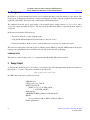
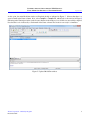
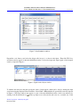
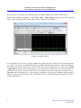
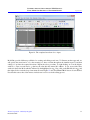
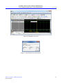
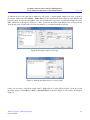
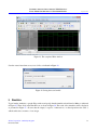
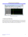
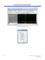
Introduction to Simulation of
VHDL Designs Using ModelSim
Graphical Waveform Editor
For Quartus II 14.1
1
Introduction
This tutorial provides an introduction to simulation of logic circuits using the Graphical Waveform Editor in the
ModelSim Simulator. It shows how the simulator can be used to perform functional simulation of a circuit specified
in VHDL hardware description language. It is intended for a student in an introductory course on logic circuits, who
has just started learning this material and needs to acquire quickly a rudimentary understanding of simulation.
Contents:
• Design Project
• Creating Waveforms for Simulation
• Simulation
• Making Changes and Resimulating
• Concluding Remarks
Altera Corporation - University Program
December 2014
1
I NTRODUCTION TO S IMULATION OF VHDL D ESIGNS
U SING M ODEL S IM G RAPHICAL WAVEFORM E DITOR
2
For Quartus II 14.1
Background
ModelSim is a powerful simulator that can be used to simulate the behavior and performance of logic circuits. This
tutorial gives a rudimentary introduction to functional simulation of circuits, using the graphical waveform editing
capability of ModelSim. It discusses only a small subset of ModelSim features.
The simulator allows the user to apply inputs to the designed circuit, usually referred to as test vectors, and to
observe the outputs generated in response. The user can use the Waveform Editor to represent the input signals as
waveforms.
In this tutorial, the reader will learn about:
• Test vectors needed to test the designed circuit
• Using the ModelSim Graphical Waveform Editor to draw test vectors
• Functional simulation, which is used to verify the functional correctness of a synthesized circuit
This tutorial is aimed at the reader who wishes to simulate circuits defined by using the VHDL hardware description
language. An equivalent tutorial is available for the user who prefers the Verilog language.
PREREQUISITE
The reader is expected to have access to a computer that has ModelSim-SE software installed.
3
Design Project
To illustrate the simulation process, we will use a very simple logic circuit that implements the majority function of
three inputs, x 1 , x 2 and x 3 . The circuit is defined by the expression
f (x 1 , x 2 , x 3 ) = x 1 x 2 + x 1 x 3 + x 2 x 3
In VHDL, this circuit can be specified as follows:
LIBRARY ieee ;
USE ieee.std_logic_1164.all ;
ENTITY majority IS
PORT ( x1, x2, x3 : IN STD_LOGIC ;
f : OUT STD_LOGIC) ;
END majority;
ARCHITECTURE LogicFunction OF majority IS
BEGIN
f <= (x1 AND x2) OR (x1 AND x3) OR (x2 AND x3);
END LogicFunction;
2
Altera Corporation - University Program
December 2014
I NTRODUCTION TO S IMULATION OF VHDL D ESIGNS
U SING M ODEL S IM G RAPHICAL WAVEFORM E DITOR
For Quartus II 14.1
Enter this code into a file called majority.vhd.
ModelSim performs simulation in the context of projects – one project at a time. A project includes the design files
that specify the circuit to be simulated. We will first create a directory (folder) to hold the project used in the tutorial.
Create a new directory and call it modelsim_intro. Copy the file majority.vhd into this directory.
Open the ModelSim simulator. In the displayed window select File > New > Project, as shown in Figure 1.
Figure 1. The ModelSim window.
A Create Project pop-up box will appear, as illustrated in Figure 2. Specify the name of the project; we chose the
name majority. Use the Browse button in the Project Location box to specify the location of the directory that you
created for the project. ModelSim uses a working library to contain the information on the design in progress; in the
Default Library Name field we used the name work. Click OK.
Altera Corporation - University Program
December 2014
3
I NTRODUCTION TO S IMULATION OF VHDL D ESIGNS
U SING M ODEL S IM G RAPHICAL WAVEFORM E DITOR
For Quartus II 14.1
Figure 2. Created Project window.
In the pop-up window in Figure 3, click on Add Existing File and add the file majority.vhd to the project as shown
in Figure 4. Click OK, then close the windows.
Figure 3. Add Items window.
Figure 4. Add Items window.
4
Altera Corporation - University Program
December 2014
I NTRODUCTION TO S IMULATION OF VHDL D ESIGNS
U SING M ODEL S IM G RAPHICAL WAVEFORM E DITOR
For Quartus II 14.1
At this point, the main Modelsim window will include the file as indicated in Figure 5. Observe that there is a
question mark in the Status column. Now, select Compile > Compile All, which leads to the window in Figure 6
indicating in the Transcript window (at the bottom) that the circuit in the majority.vhd file was successfully compiled.
Note that this is also indicated by a check mark in the Status column. The circuit is now ready for simulation.
Figure 5. Updated ModelSim window.
Altera Corporation - University Program
December 2014
5
I NTRODUCTION TO S IMULATION OF VHDL D ESIGNS
U SING M ODEL S IM G RAPHICAL WAVEFORM E DITOR
For Quartus II 14.1
Figure 6. ModelSim window after compilation.
4
Creating Waveforms for Simulation
To perform simulation of the designed circuit, it is necessary to enter the simulation mode by selecting Simulate >
Start Simulation. This leads to the window in Figure 7.
6
Altera Corporation - University Program
December 2014
I NTRODUCTION TO S IMULATION OF VHDL D ESIGNS
U SING M ODEL S IM G RAPHICAL WAVEFORM E DITOR
For Quartus II 14.1
Figure 7. Start Simulation window.
Expand the work directory and select the design called majority, as shown in the figure. Then click OK. Now,
an Objects window appears in the main ModelSim window. It shows the input and output signals of the designed
circuit, as depicted in Figure 8.
Figure 8. Signals in the Objects window.
To simulate the circuit we must first specify the values of input signals, which can be done by drawing the input
waveforms using the Graphical Waveform Editor. Select View > Wave which will open the Wave window depicted
in Figure 9. The Wave window may appear as a part of the main ModelSim window; in this case undock it by
clicking on the Dock/Undock icon
in the top right corner of the window and resize it to a suitable size. If the
Altera Corporation - University Program
December 2014
7
I NTRODUCTION TO S IMULATION OF VHDL D ESIGNS
U SING M ODEL S IM G RAPHICAL WAVEFORM E DITOR
For Quartus II 14.1
Wave window does not appear after undocking, then select View > Wave in the main ModelSim window.
We will run the simulation for 800 ns; so, select View > Zoom > Zoom Range and in the pop-up window that will
appear specify the range from 0 to 800 ns. This should produce the image in Figure 9.
Figure 9. The Wave window.
For our simple circuit, we can do a complete simulation by applying all eight possible valuations of the input signals
x 1 , x 2 and x 3 . The output f should then display the logic values defined by the truth table for the majority function.
We will first draw the waveform for the x 1 input. In the Objects window, right-click on x1. Then, choose Modify
> Apply Wave in the drop-down box that appears, as shown in Figure 10. This leads to the window in Figure 11,
which makes it possible to specify the value of the selected signal in a time period that has to be defined. Choose
Constant as the desired pattern, zero as the start time, and 400 ns as the end time. Click Next. In the window in
Figure 12, enter 0 as the desired logic value. Click Finish. Now, the specified signal appears in the Wave window,
as indicated in Figure 13.
8
Altera Corporation - University Program
December 2014
I NTRODUCTION TO S IMULATION OF VHDL D ESIGNS
U SING M ODEL S IM G RAPHICAL WAVEFORM E DITOR
For Quartus II 14.1
Figure 10. Selecting a signal in the Objects window.
Figure 11. Specifying the type and duration of a signal.
Altera Corporation - University Program
December 2014
9
I NTRODUCTION TO S IMULATION OF VHDL D ESIGNS
U SING M ODEL S IM G RAPHICAL WAVEFORM E DITOR
For Quartus II 14.1
Figure 12. Specifying the value of a signal.
Figure 13. The updated Wave window.
To draw the rest of the x 1 signal, right-click on its name in the Wave window. In the drop-down window that appears,
select Edit > Create/Modify Waveform. This leads again to the window in Figure 11. Now, specify 400 ns as the
start time and 800 ns as the end time. Click Next. In the window in Figure 12, specify 1 as the required logic value.
Click Finish. This completes the waveform for x 1 , as displayed in Figure 14.
10
Altera Corporation - University Program
December 2014
I NTRODUCTION TO S IMULATION OF VHDL D ESIGNS
U SING M ODEL S IM G RAPHICAL WAVEFORM E DITOR
For Quartus II 14.1
Figure 14. The completed waveform for x 1 input.
ModelSim provides different possibilities for creating and editing waveforms. To illustrate another approach, we
will specify the waveform for x 2 by first creating it to have a 0 value throughout the simulation period, and then
editing it to produce the required waveform. Repeat the above procedure, by right-clicking on x2 in the Objects
window, to create a waveform for x 2 that has the value 0 in the interval 0 to 800 ns. So far, we used the Wave
window in the Select Mode which is indicated by the highlighted icon . Now, click on the Edit Mode icon , and
then right-click to reach the drop-down menu shown in Figure 15 and select Wave Edit if it has not been checked.
Note that this causes the toolbar menu to include new icons for use in the editing process.
Altera Corporation - University Program
December 2014
11
I NTRODUCTION TO S IMULATION OF VHDL D ESIGNS
U SING M ODEL S IM G RAPHICAL WAVEFORM E DITOR
For Quartus II 14.1
Figure 15. Selecting the Wave Edit mode.
The waveform for x 2 should change from 0 to 1 at 200 ns, then back to 0 at 400 ns, and again to 1 at 600 ns. Select
x2 for editing by clicking on it. Then, click just to the right of the 200-ns point, hold the mouse button down and
sweep to the right until you reach the 400-ns point. The chosen interval will be highlighted in white, as shown in
Figure 16. Observe that the yellow cursor line appears and moves as you sweep along the time interval. To change
the value of the waveform in the selected interval, click on the Invert icon as illustrated in the figure. A pop-up box in
Figure 17 will appear, showing the start and end times of the selected interval. If the displayed times are not exactly
200 and 400 ns, then correct them accordingly and click OK. The modified waveform is displayed in Figure 18. Use
the same approach to change the value of x 2 to 1 in the interval from 600 to 800 ns, which should yield the result in
Figure 19.
12
Altera Corporation - University Program
December 2014
I NTRODUCTION TO S IMULATION OF VHDL D ESIGNS
U SING M ODEL S IM G RAPHICAL WAVEFORM E DITOR
For Quartus II 14.1
Figure 16. Editing the waveform.
Figure 17. Specifying the exact time interval.
Altera Corporation - University Program
December 2014
13
I NTRODUCTION TO S IMULATION OF VHDL D ESIGNS
U SING M ODEL S IM G RAPHICAL WAVEFORM E DITOR
For Quartus II 14.1
Figure 18. The modified waveform.
Figure 19. Completed waveforms for x 1 and x 2 .
We will use a third approach to draw the waveform for x 3 . This signal should alternate between 0 and 1 logic values
at each 100-ns interval. Such a regular pattern is indicative of a clock signal that is used in many logic circuits.
14
Altera Corporation - University Program
December 2014
I NTRODUCTION TO S IMULATION OF VHDL D ESIGNS
U SING M ODEL S IM G RAPHICAL WAVEFORM E DITOR
For Quartus II 14.1
To illustrate how a clock signal can be defined, we will specify x 3 in this manner. Right-click on the x 3 input in
the Objects window and select Modify > Apply Wave. In the Create Pattern Wizard window, select Clock as the
required pattern, and specify 0 and 800 ns as the start and end times, respectively, as indicated in Figure 20. Click
Next, which leads to the window in Figure 21. Here, specify 0 as the initial value, 200 ns as the clock period, and
50 as the duty cycle. Click Finish. Now, the waveform for x 3 is included in the Wave window.
Figure 20. Selecting a signal of clock type.
Figure 21. Defining the characteristics of a clock signal.
Lastly, it is necessary to include the output signal f . Right-click on f in the Objects window. In the drop-down
menu that appears, select Add to > Wave > Selected Signals as shown in Figure 22. The result is the image in
Figure 23.
Altera Corporation - University Program
December 2014
15
I NTRODUCTION TO S IMULATION OF VHDL D ESIGNS
U SING M ODEL S IM G RAPHICAL WAVEFORM E DITOR
For Quartus II 14.1
Figure 22. Adding a signal to the Wave window.
16
Altera Corporation - University Program
December 2014
I NTRODUCTION TO S IMULATION OF VHDL D ESIGNS
U SING M ODEL S IM G RAPHICAL WAVEFORM E DITOR
For Quartus II 14.1
Figure 23. The completed Wave window.
Save the created waveforms as majority.do file, as indicated in Figure 24.
Figure 24. Saving the waveform file.
5
Simulation
To perform the simulation, open the Wave window and specify that the simulation should run for 800 ns, as indicated
in Figure 25. Then, click on the Run-All icon, as shown in Figure 26. The result of the simulation will be displayed
as presented in Figure 27. Observe that the output f is equal to 1 whenever two or three inputs have the value 1,
which verifies the correctness of our design.
Altera Corporation - University Program
December 2014
17
I NTRODUCTION TO S IMULATION OF VHDL D ESIGNS
U SING M ODEL S IM G RAPHICAL WAVEFORM E DITOR
For Quartus II 14.1
Figure 25. Setting the simulation interval.
Figure 26. Running the simulation.
18
Altera Corporation - University Program
December 2014
I NTRODUCTION TO S IMULATION OF VHDL D ESIGNS
U SING M ODEL S IM G RAPHICAL WAVEFORM E DITOR
For Quartus II 14.1
Figure 27. Result of the simulation.
6
Making Changes and Resimulating
Changes in the input waveforms can be made using the approaches explained above. Then, it is necessary to resimulate the circuit using the altered waveforms. For example, change the waveform for x 1 to have the logic value 1
in the interval from 0 to 200 ns, as indicated in Figure 28. Now, click on the Restart icon shown in the figure. A
pop-up box in Figure 29 will appear. Leave the default entries and click OK. Upon returning to the Wave window,
simulate the design again by clicking on the Run-All icon. The result is given in Figure 30.
Altera Corporation - University Program
December 2014
19
I NTRODUCTION TO S IMULATION OF VHDL D ESIGNS
U SING M ODEL S IM G RAPHICAL WAVEFORM E DITOR
For Quartus II 14.1
Figure 28. Changed input waveforms.
Figure 29. The Restart box.
20
Altera Corporation - University Program
December 2014
I NTRODUCTION TO S IMULATION OF VHDL D ESIGNS
U SING M ODEL S IM G RAPHICAL WAVEFORM E DITOR
For Quartus II 14.1
Figure 30. Result of the new simulation.
Simulation is a continuous process. It can be stopped by selecting Simulate > End Simulation in the main ModelSim window.
7
Concluding Remarks
The purpose of this tutorial is to provide a quick introduction to ModelSim, explaining only the rudimentary aspects
of functional simulation that can be performed using the ModelSim Graphical User Interface. More details about
the ModelSim GUI and its use in simulation can be found in the Generating Stimulus with Waveform Editor chapter
of ModelSim SE User’s Manual, which is available as part of an installed ModelSim-SE simulator.
A more extensive discussion of simulation using the ModelSim simulator is provided in the tutorial Using ModelSim
to Simulate Logic Circuits for Altera Devices, which is available on Altera’s University Program Web site.
Altera Corporation - University Program
December 2014
21
I NTRODUCTION TO S IMULATION OF VHDL D ESIGNS
U SING M ODEL S IM G RAPHICAL WAVEFORM E DITOR
For Quartus II 14.1
Copyright ©1991-2014 Altera Corporation. All rights reserved. Altera, The Programmable Solutions Company, the
stylized Altera logo, specific device designations, and all other words and logos that are identified as trademarks
and/or service marks are, unless noted otherwise, the trademarks and service marks of Altera Corporation in the
U.S. and other countries. All other product or service names are the property of their respective holders. Altera
products are protected under numerous U.S. and foreign patents and pending applications, mask work rights, and
copyrights. Altera warrants performance of its semiconductor products to current specifications in accordance with
Altera’s standard warranty, but reserves the right to make changes to any products and services at any time without
notice. Altera assumes no responsibility or liability arising out of the application or use of any information, product,
or service described herein except as expressly agreed to in writing by Altera Corporation. Altera customers are
advised to obtain the latest version of device specifications before relying on any published information and before
placing orders for products or services.
This document is being provided on an “as-is” basis and as an accommodation and therefore all warranties, representations or guarantees of any kind (whether express, implied or statutory) including, without limitation, warranties
of merchantability, non-infringement, or fitness for a particular purpose, are specifically disclaimed.
22
Altera Corporation - University Program
December 2014