Download STAMP User's Guide v2.0.0

STAMP User’s Guide v2.0.0
Statistical Analysis of Metagenomic Profiles
Donovan Parks and Robert Beiko
August 10, 2011
Contents
1.
Introduction ........................................................................................................................................................2
2.
Contact information ...........................................................................................................................................2
3.
Citing STAMP and statistical techniques ............................................................................................................2
4.
Installation ..........................................................................................................................................................2
4.1 Precompiled binaries for Microsoft Windows..................................................................................................2
4.2 Source code ......................................................................................................................................................3
4.3 Unit tests: Verifying the installation .................................................................................................................3
5. Constructing and obtaining metagenomic profiles ................................................................................................3
5.1 Creating your own metagenomic profiles ........................................................................................................3
5.2 Creating a metadata file ...................................................................................................................................4
5.3 Obtaining profiles from MG-RAST ....................................................................................................................4
5.4 Obtaining profiles from IMG/M .......................................................................................................................4
5.5 Obtaining profiles from CoMet or RITA ............................................................................................................5
6. Analyzing metagenomic profiles ............................................................................................................................5
6.1 Analyzing multiple groups ................................................................................................................................5
Setting statistical analysis properties: ................................................................................................................5
Graphical exploration of results: ........................................................................................................................8
Tabular view of results: ......................................................................................................................................9
6.2 Analyzing two groups .................................................................................................................................... 12
Setting statistical analysis properties: ............................................................................................................. 12
Graphical exploration of results: ..................................................................................................................... 13
Tabular view of results: ................................................................................................................................... 13
6.3 Analyzing two samples .................................................................................................................................. 14
Setting statistical analysis properties: ............................................................................................................. 15
Graphical exploration of results: ..................................................................................................................... 16
Tabular view of results: ................................................................................................................................... 18
7. Global preferences .............................................................................................................................................. 20
8. Command-line interface ...................................................................................................................................... 20
9. Custom statistical techniques and plots .............................................................................................................. 22
9.1 Creating a custom plot .............................................................................................................................. 22
9.2 Making a plugin publicly available ............................................................................................................. 23
References ............................................................................................................................................................... 24
Page | 1
1. Introduction
STAMP (STatistical Analysis of Metagenomic Profiles) is a software package for analyzing metagenomic profiles,
such as phylogenetic profiles indicating the number of marker genes assigned to different taxonomic units or
functional profiles indicating the number of sequences assigned to different subsystems or pathways. It aims to
promote ‘best practices’ in selecting statistical techniques and in reporting results by encouraging the use of
effect sizes and confidence intervals for assessing biological importance. A user-friendly, graphical interface
permits easy exploration of statistical results and generation of publication-quality plots for inferring the
biological relevance of features in a metagenomic profile. STAMP is open-source, extensible via a plugin
framework, and available for all major platforms.
2. Contact information
STAMP is in active development and we are interested in discussing all potential applications of this software.
We encourage you to send us suggestions for new features. Suggestions, comments, and bug reports can be
sent to Rob Beiko (beiko [at] cs.dal.ca). If reporting a bug, please provide as much information as possible and a
simplified version of the data set which causes the bug. This will allow us to quickly resolve the issue.
3. Citing STAMP and statistical techniques
If you use STAMP in your research, please cite:
Parks, D.H. and Beiko, R.G (2010). Identifying biologically relevant differences between metagenomic
communities. Bioinformatics, 26, 715-721.
If you make use of White’s non-parametric t-test, please cite:
White, J.R., Nagarajan, N., and Pop, M. (2009). Statistical methods for detecting differentially abundant
features in clinical metagenomic samples. PLoS Comput Biol, 5, e1000352.
Citations for other statistics are given in Tables 1, 2, and 3.
4. Installation
4.1 Precompiled binaries for Microsoft Windows
A precompiled binary is available for Microsoft Windows. This binary has been tested under Windows XP and
Windows 7, but should also work under Windows Vista. The precompiled binary is available from the STAMP
website:
http://kiwi.cs.dal.ca/Software/STAMP
If you have a pristine copy of Microsoft Windows installed, you may need to install the Visual C++ 2008
Redistributable Package:
Page | 2
Windows XP or x86 (32-bit) versions of Windows Vista or 7
x64 (64-bit) versions of Windows Vista or 7
This package contains a number of commonly required runtime components which you likely already have via
other installed software. STAMP will fail with a message indicating the "configuration is incorrect" if you require
this package.
4.2 Source code
Running from source is the best way to fully exploit and contribute to STAMP. It is relatively simple to setup
STAMP from source on Microsoft Windows, Apple OS X, or Linux. Instructions on installing STAMP from source
are available on our wiki:
http://kiwi.cs.dal.ca/Software/Quick_installation_instructions_for_STAMP
If you wish to use STAMP strictly from the command-line (e.g., as typical of a cluster environment) only a subset
of the 3rd-party dependencies are required as detailed on the wiki.
4.3 Unit tests: Verifying the installation
A set of unit tests are available to verify that STAMP and all 3rd-party libraries are installed correctly. These unit
tests verify the numerical accuracy of the statistical tests, effect size measures, confidence interval methods,
and multiple test correction methods provided within STAMP. Executing the unit tests is strongly recommended
when installing STAMP from source. To execute the unit tests, move to the main STAMP directory and enter the
following command:
python STAMP_test.py –v
If any of these tests fail, STAMP should not be used. Please contact the authors so we can try to resolve the
situation.
5. Constructing and obtaining metagenomic profiles
5.1 Creating your own metagenomic profiles
STAMP reads text files in tab-separated values (tsv) format. This file can contain hierarchical and profile
information for two or more samples. The first row of the file contains the header for each column. Columns
indicating the hierarchical structure of a feature must be placed from the highest to lowest level in the
hierarchy. There are no restrictions on the depth of the hierarchy. Hierarchies can be multifuricating, but must
form a strict tree structure. The number of reads assigned to each leaf node in the hierarchy must be specified
for each sample. To allow for different normalization methods, these read counts may be integers or any real
number. An example input files is given below:
Page | 3
Hierarchical Level 1
Category A
Category A
Category A
Category B
Category C
Category C
Hierarchical Level 2
Subcategory A1
Subcategory A1
Subcategory A2
Subcategory B1
Subcategory C1
Subcategory C1
Sample 1
0
3
4.8
2
1
7.2
Sample 2
4.4
5
3.5
32
2
6
Sample 3
4
5
2
6.5
2
4
5.2 Creating a metadata file
STAMP allows additional data associated with each sample to be defined through a metadata file. Like a STAMP
profile, a metadata file is a tab-separated values (tsv) file. The first column of this file indicates the name of each
sample and should correspond to an entry in the corresponding STAMP profile. Additional columns can specify
any other data relevant to the samples being considered. Within STAMP, these additional columns can be used
to define groups (i.e., collections of one or more profiles) over which statistics can be calculated. For example, a
metadata file for the example profile above could have the structure:
Sample Id
Sample 1
Sample 2
Sample 3
Location
Canada
Canada
Italy
Phenotype
Obese
Lean
Lean
Gender
Female
Male
Female
Sample Size
4000
2000
3000
5.3 Obtaining profiles from MG-RAST
STAMP provides support for analyzing MG-RAST taxonomic or functional profiles. Visit the MG-RAST website
(Meyer et al., 2008; http://metagenomics.nmpdr.org) and browse the list of pubic metagenomes. Profiles for
multiple samples can be obtained and downloaded as tab-separated values (tsv) file using the table data
visualization. To work with MG-RAST profiles, they must be converted into a STAMP-compatible profile. From
within STAMP, select the Create profile from...->MG-RAST profile command from the File menu.
This opens up the Create profile dialog box. Click on the Load profile button and select the MG-RAST
profile you wish to convert. If desired, you can customize the headings of each hierarchical level by clicking on
the Customize headings button. Click the Create STAMP profile button and save the STAMP profile to a
suitable location. If you wish to give the samples more descriptive names, you can manually edit the resulting
STAMP profile in a text editor.
5.4 Obtaining profiles from IMG/M
Metagenomic profiles can also be obtained from the JGI IMG/M web portal (Markowitz et al., 2008;
http://img.jgi.doe.gov/m). Profiles for multiple samples can be created using the services at IMG/M and
downloaded as a single file. STAMP works directly with IMG/M’s abundance profiles obtained by clicking on the
Compare Genomes menu item, followed by Abundance Profile, and finally Overview (All
Functions). Select the Matrix output type with the Gene count or Estimated gene copies option
along with all metagenomes you are interested in. Hit GO and download the resulting tab-delimited file. This file
can be directly read by STAMP. Although this file has the extension xls, it is in fact a simple tab-separated
values file and you may wish to change the extension to tsv.
Page | 4
COG profiles from IMG/M do not contain information about which COG category or higher level class a COG
belongs to. STAMP can add this information to an IMG/M COG profile. This is done in the Assign COG
categories to IMG/M profile dialog accessible through the File menu. Some COGs are associated with
multiple COG categories. For example, COG0059 is assigned to COG categories E and H. You can elect to treat
multi-code COGs as unique features (i.e., there should be a COG code named EH) or to assign sequences
associated with a multi-code COG to each individual COG category (i.e., a sequence assigned to COG0059 will
add a single count to COG categories E and H).
You can create your own COG profiles and have STAMP assigned higher level COG information to your profile.
The example file Assign_COGs_Example.tsv demonstrates the required file format for using the Assign
COG categories to IMG/M profile feature of STAMP.
5.5 Obtaining profiles from CoMet or RITA
STAMP can also process the functional profiles produced by CoMet (Lingner et al., 2011) or the taxonomic
profiles produced by RITA (MacDonald et al., 2011). These web servers are available at:
CoMet: http://comet.gobics.de
RITA: http://ratite.cs.dal.ca/rita
Like MG-RAST profiles, these profiles must be converted into STAMP-compatible profiles using the appropriate
Create profile from... command within the File menu. STAMP combines multiple CoMet or RITA
profile files into a single STAMP profile file. For RITA profiles, the desired classification groups to use for profile
construction can be specified.
6. Analyzing metagenomic profiles
Taxonomic profiles of the gut microbiota of 41 individuals will be used to illustrate how STAMP can be used to
analyze metagenomic profiles. These profiles are based on the analysis performed by Arumugam et al. (2011)
which revealed that these profiles could be assigned to three distinct clusters or enterotypes. STAMPcompatible profiles and metadata for this dataset can be found in the examples/EnterotypesArumugam
directory.
6.1 Analyzing multiple groups
Setting statistical analysis properties: The enterotypes data can be loaded through the File->Load
data… dialog. Make sure to specify both the profile (Enterotypes.profile.spf) and group metadata
(Enterotypes.metadata.tsv) files before hitting OK to continue. Here we will group the data by the three
enterotypes specified by Arumugam et al. (2011). Profiles are assigned to groups through the Group legend
window. To open this window, select View->Group legend. The Group legend window can be left as a
floating window or docked in different positions (Figure 1). For this analysis, dock the window on the right
(Figure 1b) and select Enterotype from the Group field combobox. This indicates that we wish to group
the data by enterotypes. If you open the file Enterotypes.metadata.tsv you can see that Enterotype is
Page | 5
simply a column in this file. A large number of enterotypes have been defined. To replicate the analysis by
Arumugam et al. uncheck all groups except Enterotype 1, Enterotype 2, and Enterotype 3 (Figure 2).
Unchecking a group causes it to be ignored when calculating statistics and generating plots.
Notice that all statistics and plots are automatically updated as you uncheck each group. In general, STAMP
automatically regenerates all statistics and plots as needed. For large datasets this can be inconvenient. To
prevent automatic updating of results, click the Recalculate statistics and plot button in the lower,
right of the main window. Once you have modified all desired properties (e.g., selected specific groups, changed
desired statistical properties, or set appropriate filtering constraints) click the Recalculate statistics and
plot button to regenerate results.
Figure 1: Example of a floating (a) and docked (b) group legend. All windows available from the View menu can be left as
floating or docked in different positions within the main window.
Page | 6
Figure 2: Group legend specifying that profiles should be grouped according to their Enterotype. Unchecked groups have been
removed from the analysis.
Statistical properties are set through the Properties window. By default, this window is docked on the right.
However, it can be detached from this position and docked in different locations just like the Group legend
window. Windows can be selectively shown and
hidden using their corresponding entry in the View
menu. The Properties window allows you to set a
number of properties related to performing multiple
group tests. These are described below (Figure 3):
Parent level: the proportion of sequences assigned
to a feature will be calculated relative to the total
number of sequences assigned to its parent
category. The default is to calculate proportions
relative to all assigned sequences in the sample. For
this tutorial, keep the parent level at the default
value of Entire sample.
Profile level: the hierarchical level at which to
construct the profile. This allows data to be explored
at different depths in the hierarchy. For this tutorial,
change the profile level to Genera.
Unclassified: specifies how unclassified sequences
are to be handled. Any reads assigned to a feature
with the name unclassified (case insensitive) are
deemed to be unclassified. Unclassified sequences
can either be retained in the profile (Retain
unclassified reads), removed from the profile
Page | 7
(Remove unclassified reads), or removed from consideration except when calculating a profile (Use
only for calculating frequency profiles). These three options for treating unclassified sequences
can result in large differences. For both the Retain unclassified reads and Use only for
calculating frequency profiles options, the relative proportion of sequences assigned to a feature is
proportional to the total number of sequences within the specified parent category. The latter option prevents
the unclassified feature for appearing in tables and plots. In contrast, the Remove unclassified reads
option results in profiles indicating the relative proportion of sequences within each feature relative to those
sequences which were classified at the specified profile level. Since the proportion of unclassified sequences can
vary significantly between samples, this can result in vastly different profiles.
Statistical properties: the statistical test, post-hoc test along with the confidence interval width, effect size, and
multiple test correction method to use can all be specified in this section. A list of methods provided in STAMP
for analyzing multiple groups is given in Table 1.
Filtering: the filtering section provides a number of filters for identifying features that satisfy a set of criteria
(i.e., desired p-value and effect size). The number of features passing the specified filters is indicated at the
bottom of this section. In order to allow specific features to be investigated, STAMP also supports selecting
subsets of features. Feature selection is performed using the Select features dialog box which is accessed
by clicking on the Select features button. Within this dialog individual features or all features within specific
parent categories can be selected or removed from consideration. Filtering is performed on these selected
features in order to allow investigating specific subsets of features with particular properties. To investigate a
subset of features without performing any filtering uncheck all the filters.
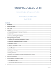
Graphical exploration of results: The following plots are provided for exploring the results of a multiple
groups analysis:



Bar plot: a bar plot indicating the proportion of sequences assigned to each feature. The feature to plot
is selected from a table to the right of the plot (Figure 3). This table can be moved in and out to provide
additional space for the plot. Table columns can be sorted to focus on features with low p-values or
large effect sizes. Additionally, the table can be limited to those features passing the specified filters by
checking the Show only active features checkbox. The example in Figure 3 shows the proportion
of Bacteroides within each sample and reveals the over-abundance of this genus within Enterotype 1.
Arumugam et al. (2011) also suggested Prevotella and Ruminococcus as genera useful for distinguishing
between enterotypes.
Box plot: a box plot is similar to a bar plot except the distribution of proportions within a group are
indicated using a box-and-whiskers graphic (Figure 4). This provides a more concise summary of the
distribution of proportions within a group. The box-and-whiskers graphics show the median of the data
as a line, the mean of the data as a star, the 25th and 75th percentiles of the data as the top and bottom
of the box, and uses whiskers to indicate the most extreme data point within 1.5*(75th – 25th percentile)
of the median. Data points outside of the whiskers are shown as crosses.
PCA plot: a principal component analysis (PCA) plot of the samples. Clicking on a marker within the plot
indicates the sample represented by the marker.
Page | 8

Post-hoc plot: the null hypothesis of a multiple group statistic test (i.e., ANOVA or Kruskal-Wallis) is that
the means of all groups are equal. Given a p-value sufficiently small to suggest this null hypothesis
should be rejected, we can only conclude that the means of all groups are not equal. If we wish to
identify which pairs of groups may differ from each other a post-hoc test must be performed. A post-hoc
plot shows the results of such a test. It provides a p-value and effect size measure for each pair of
groups (Figure 5). In the case of Bacteroides, the mean abundance in Enterotype 1 is found to differ
significantly from the mean abundance in Enterotypes 2 and 3. (p ≤ 0.001) In contrast, the mean
abundance in Enterotypes 2 and 3 do not differ significantly (p ≥ 0.1).
Each of these plots provides a number of customization options. To customize a plot, click the Configure
plot button below the plot. Plots can also be sent to a new window using the Send plot to window
command under the View menu. This allows multiple plots to be viewed at once. Plots can be saved in
raster (PNG) and vector (PDF, PS, EPS, SVG) formats (File->Save plot…). For raster formats the desired
resolution can be specified.
Tabular view of results: the results of a multiple groups analysis are tabulated in a Multiple group
statistics table. This table is accessed through the View->Multiple group statistics table
menu item. The resulting table can be docked or left as a floating window. Columns can be sorted to help
identify patterns of interest. Results can be limited to only the active features (those passing the specified filters)
by checking the Show only active features checkbox. The table can be saved to file using the Save
button. Tables are saved as text files in tab-separated values format which can be read by any text editor and
most spreadsheet programs.
Figure 3. Bar plot showing the relative proportion of Bacteriodes within 32 gut microbiota samples. Samples are coloured
according to the enterotype to which they have been assigned. The table on the right provides a list of features (genera) which
can be plotted. It has been sorted by increasing order of p-values. Bacteriodes has the smallest p-value of all genera.
Page | 9
Figure 4. Box plot showing the distribution in the proportion of Bacteriodes assigned to samples from three enterotypes. Boxes
th
th
indicate the IQR (75 to 25 of the data). The median value is shown as a line within the box and the mean value as a star.
Whiskers extend to the most extreme value within 1.5*IQR. Outliers are shown as crosses.
Figure 5. Post-hoc plot for Bacteriodes indicating 1) the mean proportion of sequences within each enterotype, 2) the
difference in mean proportions for each pair of enterotypes, and 3) a p-value indicating if the mean proportion is equal for a
given pair.
Page | 10
Statistical hypothesis tests
Comments
References
ANOVA
An analysis of variance (ANOVA) is a method for testing whether or
not the means of several groups are all equal. It can be seen as a
generalization of the t-test to more than two groups.
A non-parametric method for testing whether or not the median
of several groups are all equal. It considers the rank order of each
sample and not the actual proportion of sequences associated
with a feature. This has the benefit of not assuming the data is
normally distributed. Each group must contain at least 5 samples
to apply this test.
Bluman, 2007
Kruskal-Wallis H-test
Post-hoc tests
Games-Howell
Scheffè
Tukey-Kramer
Welch’s (uncorrected)
Used to determine which means are significantly different when
an ANOVA produces a significant p-value. This post-hoc test is
designed for use when variances and group sizes are unequal. It is
preferable to Tukey-Kramer when variances are unequal and group
sizes are small, but it more computationally expensive.
A general post-hoc test for considering all possible contrasts unlike
the Tukey-Kramer method which considers only pairs of means.
Currently, STAMP only considers pairs of means so the TukeyKramer method is preferred. In general, this test is highly
conservative.
Used to determine which means are significantly different when
an ANOVA produces a significant p-value. It considers all possible
pairs of means while controlling the familywise error rate (i.e.,
accounting for multiple comparisons). In general, we recommend
using the Games-Howell post-hoc test when reporting final results
and the Tukey-Kramer method for exploratory analysis since it is
less computationally intensive. The Tukey-Kramer may also be
preferred as it is more widely used and known amongst
researchers.
Simple performs Welch’s t-test on each possible pair of means. No
effort is made to control the familywise error rate.
Bluman, 2007
Bluman, 2007
Multiple test correction methods
Benjamini-Hochberg FDR
Initial proposal for controlling false discovery rate instead of the
Benjamini and Hochberg,
familywise error. Step-down procedure.
1995
Bonferroni
Classic method for controlling the familywise error. Often criticized
Adbi, 2007
as being too conservative.
Šidák
Less common method for controlling the familywise error rate.
Adbi, 2007
Uniformly more powerful than Bonferroni, but requires the
assumption that individual tests are independent.
Storey’s FDR
Recent method used to control the false discovery rate. More
Storey and Tibshirani, 2003
powerful than the Benjamini-Hochberg method. Requires
Storey et al., 2004
estimating certain parameters and is more computationally
expensive than the Benjamini-Hochberg approach.
Table 1. Multiple group statistical techniques available in STAMP. Our recommendations are indicated in bold.
Page | 11
6.2 Analyzing two groups
Setting statistical analysis properties: To analyze a pair of groups, click on the Two groups tab in the
Properties window. Whether analyzing multiple groups or a pair of groups, groupings are determined by the
value of the Group field combobox in the Group legend window. In this section, we will consider if there
are compositional differences in the gut microbiota of males and females by setting the Group field to
Gender.
Statistical properties are set through the Properties window. The settings for Parent level, Profile level, and
the treatment of Unclassified sequences apply uniformly to all analyses (i.e., multiple groups, two groups, and
two samples). Analysis specific properties are given below the analysis type tabs in the Properties window.
Profile: The profile section is used to specify which pair of groups will be analyzed. In this case, we have only two
groups (male and female) so we do not need to change these values. The colour associated with the two groups
can also be changed by clicking on the colour button next to these groups. Group 2 can also be set to <All
other samples> in which case all samples not contained in group 1 are used to form the second group. This is
useful for comparing a specific set of samples to all other samples within a study.
Statistical properties: the statistical test, confidence interval method and width, and multiple test correction
method to use can all be specified in this section. A one or two-sided statistical hypothesis tests can be
performed although generally a two-sided test should be used for the reasons discussed in Rivals et al. (2007). A
list of methods provided in STAMP for analyzing two groups is given in Table 2.
Filtering: the filtering section provides a large number of filters for identifying features that satisfy a set of
criteria with the number of features passing the specified filters indicated at the bottom of the section.
Attention can be focused on a specific subset of features using the Select features dialog. The provided
filters are as follows:




p-value filter: all features with a p-value greater than the specified value are removed
Sequence filter: allows features that have been assigned fewer than the specified number of sequences
to be removed. Filtering can be applied to the sample within the two groups having either the maximum
or minimum number of sequences for a given feature. Alternatively, filtering can be applied
independently to the samples within each group and features filtered if the samples within either group
contain an insufficient number of sequences.
Parent sequence filter: same as the sequence filter except applied to the sequence counts within
parental categories.
Effect size filters: allows features with small effect sizes to be removed. Filtering can be performed on
two different effect size statistics. This allows one to filter on both an absolute (i.e., difference between
proportions) and relative (i.e., ratio of proportions) measure of effect size. These filters can be applied
so features failing either condition (logical OR operator) or both conditions (logical AND operator) are
filtered. These effect size filters are applied to the mean proportions over all samples within a group.
Page | 12
Graphical exploration of results: The following plots are provided for exploring the results of a two
groups analysis:





Bar plot: a bar plot indicating the proportion of sequences assigned to each feature. The feature to plot
is selected from a table to the right of the plot.
Box plot: a box plot is similar to a bar plot except the distribution of proportions within a group are
indicated using a box-and-whiskers graphic. This provides a more concise summary of the distribution of
proportions within a group. The box-and-whiskers graphics show the median of the data as a line, the
mean of the data as a star, the 25th and 75th percentiles of the data as the top and bottom of the box,
and uses whiskers to indicate the most extreme data point within 1.5*(75th – 25th percentile) of the
median. Data points outside of the whiskers are shown as crosses.
PCA plot: a principal component analysis (PCA) plot of the samples. Clicking on a marker within the plot
indicates the sample represented by the marker.
Scatter plot: indicates the mean proportion of sequences within each group which are assigned to each
feature. This plot is useful for identifying features that are clearly enriched in one of the two groups. The
spread of the data within each group can be shown in various ways (e.g., standard deviation, minimum
and maximum proportions).
Extended error bar: indicates the difference in mean proportion between the two groups along with the
associated confidence interval of this effect size and the p-value of the specified statistical test. In
addition, a bar plot indicates the mean proportion of sequences assigned to a feature in each group. We
believe this is the minimal amount of information required to reason about the biological relevance of a
feature. Figure 6 gives an extended error bar plot for the enterotype data.
Figure 6: Extended error bar plot indicating all genera where Welch’s t-test produces a p-value > 0.1. All genera are
overabundant within the gut microbiota of males (M) compared to females (F).
Tabular view of results: the results of a two groups analysis are tabulated in a Two group statistics
table. This table is accessed through the View->Two group statistics table menu item.
Page | 13
Statistical hypothesis tests
Comments
References
t-test (equal variance)
Student’s t-test which explicitly assumes the two groups have
equal variance. When this assumption can be made, this test is
more powerful than Welch’s t-test.
A variation of Student’s t-test that is intended for use when the
two groups cannot be assumed to have equal variance.
Non-parametric test proposed by White et al. for clinical
metagenomic data. This test uses a permutation procedure to
remove the normality assumption of a standard t-test. In addition,
it uses a heuristic to identify sparse features which are handled
with Fisher’s exact test and a pooling strategy when either group
consists of less than 8 samples. See White et al., 2009 for details.
Bluman, 2007
Welch’s t-test
White’s non-parametric t-test
Confidence interval methods
DP: t-test inverted
DP: Welch’s inverted
DP: bootstrap
Bluman, 2007
White et al., 2009
Only available when using the equal variance t-test. Provides
confidence intervals by inverting the equal variance t-test.
Only available when using Welch’s t-test. Provides confidence
intervals by inverting Welch’s t-test.
Only available when using White’s non-parametric t-test. Provides
confidence intervals using a percentile bootstrapping method. If
White’s non-parametric t-test defaults to using Fisher’s exact test,
confidence intervals are obtained using the Asymptotic with CC
approach (see Table 3).
Multiple test correction methods
Benjamini-Hochberg FDR
Initial proposal for controlling false discovery rate instead of the
Benjamini and Hochberg,
familywise error. Step-down procedure.
1995
Bonferroni
Classic method for controlling the familywise error. Often criticized
Adbi, 2007
as being too conservative.
Šidák
Less common method for controlling the familywise error rate.
Adbi, 2007
Uniformly more powerful than Bonferroni, but requires the
assumption that individual tests are independent.
Storey’s FDR
Recent method used to control the false discovery rate. More
Storey and Tibshirani, 2003
powerful than the Benjamini-Hochberg method. Requires
Storey et al., 2004
estimating certain parameters and is more computationally
expensive than the Benjamini-Hochberg approach.
Table 2. Two group statistical techniques available in STAMP. Our recommendations are indicated in bold. DP = difference
between mean proportions.
Page | 14
6.3 Analyzing two samples
Setting statistical analysis properties: To analyze a pair
of samples, click on the Two samples tab in the
Properties window. In this section, we will consider if
there are compositional differences in the gut microbiota
between two twins, AM-F10-T1 and AM-F10-T2.
Profile: The profile section is used to specify which pair of
samples will be analyzed. Set the Sample 1 and Sample 2
comboboxes to AM-F10-T1 and AM-F10-T2, respectively.
The colour associated with these two samples can be
changed by clicking on the colour button next to the
samples.
Statistical properties: the statistical test, confidence interval
method and width, and multiple test correction method to
use can all be specified in this section. A one or two-sided
statistical hypothesis tests can be performed although
generally a two-sided test should be used for the reasons
discussed in Rivals et al. (2007). To assess biological
importance it is often useful to consider both an absolute
effect size statistic such as the different between proportions
and a relative statistic such as the ratio of proportions. For
the difference between proportions we recommend using
the Newcombe-Wilson method for calculating CIs and for the
ratio of proportions we recommend the standard asymptotic
approach (Parks and Beiko, 2009; Newcombe, 1998). CIs are
typically created for a nominal coverage of 95% and in
general there is little reason to deviate from this convention.
A list of methods provided in STAMP for analyzing two
samples is given in Table 3.
Filtering: the filtering section provides a large number of
filters for identifying features that satisfy a set of criteria with the number of features passing the specified
filters indicated at the bottom of the section. Attention can be focused on a specific subset of features using the
Select features dialog. The provided filters are as follows:


p-value filter: all features with a p-value greater than the specified value are removed
Sequence filter: allows features that have been assigned fewer than the specified number of sequences
to be removed. Filtering can be applied to the maximum or minimum number of sequences assigned to
a feature within the two samples. Alternatively, features can be filtered by sequence count using an
independent threshold for each sample.
Page | 15


Parent sequence filter: same as the sequence filter except applied to the sequence counts within
parental categories.
Effect size filters: allows features with small effect sizes to be removed. Filtering can be performed on
two different effect size statistics. This allows one to filter on both an absolute (i.e., difference between
proportions) and relative (i.e., ratio of proportions) measure of effect size. These filters can be applied
so features failing either condition (logical OR operator) or both conditions (logical AND operator) are
filtered.
Graphical exploration of results: STAMP contains several statistical plots to help investigate the results of a
two sample analysis and to identify features that are of biological relevance:







Profile bar plot: a bar plot indicating the proportion of sequences assigned to each feature. It is
recommended for investigating higher hierarchical levels of a profile where the number of features is
relatively small. Confidence intervals for each proportion are calculated using the Wilson score method
(Newcombe, 1998b). Figure 7 gives a profile bar plot of the two twin gut microbiota profiles.
Scatter plot: indicates the proportion of sequences assigned to each feature in a colour coded scatter
plot. This plot is useful for identifying features that are clearly enriched in one of the two samples.
Confidence intervals for each proportion can be displayed and are calculated using the Wilson score
method (Newcombe, 1998b). A notable benefit of this plot is that it can be applied to metagenomes
which have a large number of features. Figure 8 gives a profile scatter plot of the two twin gut
microbiota profiles.
Sequence histogram: gives a general overview of the number of sequences assigned to each feature.
Bar plot: the bar plot can be used to look at any statistic in detail for the set of active features (i.e., effect
size, p-value, corrected p-value, number of sequences assigned to a feature in each sample, or the
relative proportion of sequences assigned to a feature in each sample).
Extended error bar plot: indicates the p-value along with the effect size and associated confidence
interval for each active feature. In addition, a bar plot indicates the proportion of sequences assigned to
a feature in each sample. We believe this is the minimal amount of information required to reason
about the biological relevance of a feature. Figure 9 contain an extended error bar plots for the two twin
gut microbiota profiles.
Multiple comparison plot: a multiple comparison plot can be used to analyze the results of applying a
multiple test correction technique.
p-value histogram: a p-value histogram shows the distribution of p-values in a metagenomic profile.
Page | 16
Figure 7. Profile bar plot showing the relative proportion of the 30 most abundant genera in the gut microbiota of a pair of
twins.
Page | 17
Figure 8. Profile scatter plot indicating the relative proportion of all 248 genera within the gut microbiota of a pair of twins.
Detailed information for the point highlighted in red is shown in a Tooltip dialog. Detailed information about any point can be
obtained by clicking on it. Points on either side of the grey dashed y = x line are enriched in one of the two samples. A
statistical hypothesis test is required to determine if the observed difference is large enough to safely discount it being a
sampling artifact. This plot illustrates that the majority of genera within the gut microbiota are present in low proportions (i.e., <
5%) and are similar in our two samples.
Figure 9. Extended error bar plot for the four genera that have a difference between proportions of at least 3% and a ratio of
proportions of at least 2.
Tabular view of results: the results of a two sample analysis are tabulated in a Two sample statistics
table. This table is accessed through the View->Two sample statistics table menu item.
Page | 18
Statistical hypothesis tests
Comments
References
Bootstrap
A rough non-parametric approximation to Barnard’s exact test.
Assumes sampling with replacement.
Large sample approximation to Fisher’s exact test. Generally liberal
compared to Fisher’s.
Large sample approximation to Fisher’s exact test which has been
corrected to account for the discrete nature of the distribution it is
approximating. Generally conservative compared to Fisher’s.
Z-test. Large sample approximation to Barnard’s exact test.
Conditional exact test where p-values are calculated using the
‘minimum-likelihood’ approach. Computationally efficient even for
large metagenomic samples. Widely used and understood.
Large sample approximation to Fisher’s exact test. Often
considered more appropriate than the Chi-square approximation.
Generally liberal compared to Fisher’s.
Large sample approximation to Fisher’s exact test which has been
corrected to account for the discrete nature of the distribution it is
approximating. Generally conservative compared to Fisher’s.
Applied Fisher’s exact test if any entry in the contingency table is
less than 20. Otherwise, the G-test with Yates’ continuity
correction is used. For clarity, we recommend reporting final
results using just Fisher’s exact test. However, it is far more
efficient to explore the data using this hybrid statistical test.
Conditional exact test where p-values are calculated using the
‘doubling’ approach. More computationally efficient than the
‘minimum-likelihood’ approach, but the latter approach is more
commonly used by statistical packages (i.e., R and StatXact). Our
results suggest the doubling approach is generally more
conservative than the minimum-likelihood approach.
Approximation to Fisher’s exact test. Assumes sampling without
replacement.
Manly, 2007
Chi-square
Chi-square with Yates’
Difference between proportions
1
Fisher’s exact test
G-test
G-test with Yates’
G-test (w/Yates’) + Fisher’s
Hypergeometric
1
Permutation
Confidence interval methods
DP: Asymptotic
DP: Asymptotic with CC
DP: Newcombe-Wilson
OR: Haldane adjustment
RP: Asymptotic
Multiple test correction methods
Benjamini-Hochberg FDR
Standard large sample method.
As above, with a continuity correction to account for the discrete
nature of the distribution being approximated.
Method recommended by Newcombe in a comparison of seven
asymptotic approaches.
Standard large sample method with a correction to handle
degenerate cases.
Standard large sample method.
Cochran, 1952
Agresti, 1992
Yates, 1934
Agresti, 1990
Agresti, 1990
Rivals et al., 2007
Agresti, 1990
Yates, 1934
Agresti, 1990
Rivals et al., 2007
Yates, 1934
Rivals et al., 2007
Manly, 2007
Newcombe, 1998
Newcombe, 1998
Newcombe, 1998
Bland, 2000; Lawson, 2004;
Agresti, 1999
Agresti, 1990
Initial proposal for controlling false discovery rate instead of the
Benjamini and Hochberg,
familywise error. Step-down procedure.
1995
Bonferroni
Classic method for controlling the familywise error. Often criticized
Adbi, 2007
as being too conservative.
Šidák
Less common method for controlling the familywise error rate.
Adbi, 2007
Uniformly more powerful than Bonferroni, but requires the
assumption that individual tests are independent.
Storey’s FDR
Recent method used to control the false discovery rate. More
Storey and Tibshirani, 2003
powerful than the Benjamini-Hochberg method. Requires
Storey et al., 2004
estimating certain parameters and is more computationally
expensive than the Benjamini-Hochberg approach.
Table 3. Two sample statistical techniques available in STAMP. Our recommendations are indicated in bold. CC = continuity
1
correction, DP = difference between proportions, OR = odds ratio, RP = ratio of proportions. Use of Fisher’s exact test to
imply a ‘minimum-likelihood’ approach and hypergeometric to imply a ‘doubling’ approach to calculating a p-value is
commonly, but not universally, used.
Page | 19
7. Global preferences
Global user preferences can be set in the Preferences dialog
available from the Setttings menu. Within this dialog the
pseudocount to add to the unobserved data can be set.
Pseudocounts are only added when a sample has a count of
zero and the statistical method is degenerate for such
boundary cases. The only exception to this is the Haldane odds
ratio confidence interval method which adds the pseudocount
to all table entries regardless of their initial value. The default
value of 0.5 should be changed with caution. The number of
replicates to construct when performing a bootstrap or
permutation test is also set through this dialog.
Global options relevant to the generation of plots can also be
set through this dialog. Feature names within metagenomic
profiles are often relatively long. This can make producing
plots suitable for journal publication difficult. The
Preferences dialog allows feature names to be truncated to a specific length. Colour of plot axes and the
group comprising ‘all other samples’ (see Section 6.2) can also be set. Finally, p-values below a specified value
can be reported using a ‘≤’ notation to aid clarity.
8. Command-line interface
STAMP provide a command-line interface (CLI) to facilitate batch processing or ‘application linking’ as
recommended by Kumar and Dudley (2007). If you are running STAMP from source you can access the CLI by
passing parameters to commandLine.py. The precompiled binary for Microsoft Windows contains a separate CLI
executable (commandLine.exe). Table 4 lists the parameters accepted by the CLI. Command line parameters
taking the name of a statistical method (e.g., --statTest) should be given a parameter value identical to the name
of the method as it appears in the graphical user interface. This allows full support for the STAMP plugin
architecture through the CLI (see Section 9).
As an example, a two groups analysis of the enterotype data can be performed as follows:
commandLine.exe --typeOfTest "Two groups"
--profile ./examples/EnterotypesArumugam/Enterotypes.profile.spf
--metadata ./examples/EnterotypesArumugam/Enterotypes.metadata.tsv
--field Gender --name1 F --name2 M --statTest "t-test (equal variance)" --CI "DP: t-test inverted"
Results from this analysis will be written to results.tsv.
Page | 20
General parameter
--help
--version
--verbose
Profile parameters
--profile
--metadata
--field
--name1
--name2
--profLevel
Description
Information on using the STAMP command-line interface
Version information for the STAMP command-line interface
Print progress information (1) or suppress all output (0)
--parentLevel
Parental level used to calculate relative proportions
(e.g., Entire sample)
Specify treatment on unclassified fragments (Retain unclassified reads,
Remove unclassified reads, Use only for calculating frequency profiles)
--unclassifiedTreatment
Statistical parameters
--typeOfTest
--statTest
--sided
--CI
STAMP profile file to process
STAMP metadata file to process for multiple or two groups analyses
Metadata field used to define groups for multiple or two groups analyses
Name of group or sample 1 within the STAMP profile or metadata file
Name of group or sample 1 within the STAMP profile or metadata file
Hierarchical level to perform statistical analysis upon (e.g., Subsystem)
Type of test to perform (e.g., Multiple groups, Two groups, Two samples)
Statistical hypothesis test to use (e.g., Fisher’s exact test)
Perform either a one (One-sided) or two-sided (Two-sided) test
Confidence interval method to use (e.g., DP: Newcombe-Wilson)
--coverage
Nominal coverage of confidence interval (e.g., 0.95)
--multComp
Multiple comparison method to use (e.g., “Storey FDR”)
Filtering parameters
--pValueFilter
Remove features with a p-value above this threshold (e.g., 0.05)
--seqFilter
Filter to apply to counts in profile level (e.g., maximum)
--sample1Filter
Filter criteria for sample 1 (e.g., 5)
--sample2Filter
Filter criteria for sample 2 (e.g., 5)
--parentSeqFilter
Filter to apply to counts in parent level (e.g., maximum)
--parentSample1Filter
Filter criteria for sample 1 (e.g., 5)
--parentSample1Filter
Filter criteria for sample 2 (e.g., 5)
--effectSizeMeasure1
Effect size measure to filter on (e.g., “Difference between proportions”)
--minEffectSize1
Minimum required effect size for above filter (e.g., 0.5)
--effectSizeMeasure2
Effect size measure to filter on (e.g., “Ratio of proportions”)
--minEffectSize2
Minimum required effect size for above filter (e.g. 2)
--effectSizeOperator
Logical operator to apply to effect size filters (0 – OR, 1 – AND)
Output parameters
--outputTable
Filename for output table
Table 4. Command-line interface parameters accepted by STAMP. * = required parameter
Default
1
*
*
*
Lowest level in
hierarchy
Entire sample
Retain unclassified
reads
Two samples
Fisher’s exact test
Two sided
DP: NewcombeWilson
0.95
No correction
0.05
Disabled
0
0
Disabled
0
0
Disabled
0
Disabled
0
0
results.tsv
Page | 21
9. Custom statistical techniques and plots
STAMP uses a plugin architecture in order to allow new statistical hypothesis tests, effect size statistics, CI
methods, multiple comparison procedures, or plots to be easily incorporated into the software. Plugins are
written in Python and must implement a pre-defined interface as specified in an abstract base class. To have a
plugin load into STAMP it simply needs to be placed in the relevant plugin folder located at
/STAMP/library/plugins/. All statistical techniques and plots available in STAMP have been implemented as
plugins and can be consulted as examples.
9.1 Creating a custom plot
Here we will create a minimal two sample statistical plot plugin which displays a scatter plot of the relative
abundance of all active features (see STAMP/library/plugins/samples/plots/examples/MyScatterPlot.py). This
will be nearly identical to the exploratory scatter plot that indicates the relative abundance of all features. To
begin, create a file named MyScatterPlot.py in /STAMP/library/plugins/samples/plots. It is important that
you place new plugins into the correct plugins folder. To adhere to the required interface for a statistical plot
you must create a new class which is derived from AbstractSamplePlotPlugin:
class MyScatterPlot(AbstractSamplePlotPlugin):
def __init__(self, preferences, parent=None):
AbstractSamplePlotPlugin.__init__(self, preferences, parent)
self.preferences = preferences
self.name = 'My scatter plot'
self.figWidth = 6.0
self.figHeight = 6.0
self.sampleName1 = ''
self.sampleName2 = ''
The __init__ function takes two parameters. The preferences parameter indicates global user preferences
and the parent parameter indicates the parent window for your plot. You will generally want to save these
preferences in a class variable for later use. The only required class variable is name which indicates what your
plot will be called within STAMP. In the initialization function it is generally useful to initialize all class variables
to known default values.
The only other required function is plot. This function takes two parameters, profile and statsResults,
which provides details about the profiles for the two samples and the results of all calculated statistics,
respectively. Please consult the other plugins for details on how to use these two parameters. The plot function
below creates a scatter plot with each data point coloured to reflect the sample it is most abundant in.
Page | 22
def plot(self, profile, statsResults):
# Colour of plot elements
profile1Colour = str(self.preferences['Sample 1 colour'].name())
profile2Colour = str(self.preferences['Sample 2 colour'].name())
# Set sample names
if self.sampleName1 == '' and self.sampleName2 == '':
self.sampleName1 = statsResults.profile.sampleNames[0]
self.sampleName2 = statsResults.profile.sampleNames[1]
# Get data to plot
field1 = statsResults.getColumn('RelFreq1')
field2 = statsResults.getColumn('RelFreq2')
# Set figure size
self.fig.clear()
self.fig.set_size_inches(self.figWidth, self.figHeight)
axesScatter = self.fig.add_subplot(111)
# Set visual properties of all points
colours = []
for i in xrange(0, len(field1)):
if field1[i] > field2[i]:
colours.append(profile1Colour)
else:
colours.append(profile2Colour)
# Create scatter plot
axesScatter.scatter(field1, field2, c=colours)
# Update plot
self.updateGeometry()
self.draw()
For a plot to be sent to a new window the mirrorProperties function needs to be implemented. To create a
configuration dialog box for your plot the configure function must be implemented. We have been making
use of Qt Designer to create configuration dialogs which comes bundled with PyQt4. A useful exercise is to
extend this simple scatter plot so it contains all the functionality of the exploratory scatter plot
(/STAMP/library/plugins/samples/plots/ScatterPlot.py).
9.2 Making a plugin publicly available
If you have created a plugin and would like to make it publicly available, we are happy to host it on the STAMP
website. Plugins that will be of general use to STAMP users will be included in future releases (with your
permission) and attributed to you. To have a plugin hosted on the STAMP website send an email to Rob Beiko
(beiko [at] cs.dal.ca).
Page | 23
References
Adbi, H. (2007) Encyclopedia of Measurement and Statistics. Thousand Oaks, CA: Sage.
Agresti, A. (1990) Categorical data analysis., New York : Wiley.
Agresti, A. (1992) A survey of exact inference for contingency tables. Statist Sci, 7, 131–153.
Agresti, A. (1999) On logit confidence intervals for the odds ratio with small samples. Biometrics, 55, 597–602.
Arumugam, M. et al. (2011) Enterotypes of the human gut microbiome. Nature, 473, 174-180.
Benjamini, Y. and Hochberg, Y. (1995) Controlling the false discovery rate: a practical and powerful approach to
multiple testing. J Roy Stat Soc B, 57, 289–300.
Bland, J. M. and Altman, D. G. (2000) The odds ratio. BMJ, 320, 1468.
Bluman, A.G. (2007) Elementary statistics: A step by step approach (6th edition), McGraw Hill Higher Education,
New York, New York.
Cochran, W. (1952) The chi-square test of goodness of fit. Ann Math Stat, 23, 315–45.
Kumar, S. and Dudley, J. (2007) Bioinformatics software for biologists in the genomics era. Bioinformatics,
23, 1713–1717.
Lawson, R. (2004) Small sample confidence intervals for odds ratio. Commun Stat Simulat, 33, 1095–1113.
Lingner, T. et al. (2011) CoMet – a web server for comparative functional profiling of metagenomes. Nucleic
Acids Res, 39 (suppl 2), W518-W523.
MacDonald, N.J. et al. (2011) RITA: rapid identification of high-confidence taxonomic assignments for
metagenomic data. (in preparation)
Manly, B. F. J. (2007) Randomization, bootstrap and Monte Carlo methods in biology, Physica Verlag, An Imprint
of Springer-Verlag GmbH.
Markowitz, V. M. et al. (2008) IMG/M: a data management and analysis system for metagenomes. Nucleic Acids
Res, 36 (Database issue), D534–D538.
Meyer, F. et al. (2008) The metagenomics rast server - a public resource for the automatic phylogenetic and
functional analysis of metagenomes. BMC Bioinformatics, 9, 386.
Newcombe, R. G. (1998) Interval estimation for the difference between independent proportions: comparison of
eleven methods. Stat Med., 17, 873–890.
Newcombe, R.G. (1998b) Two-sided confidence intervals for the single proportion; comparison of several
methods. Stat Med., 17, 857-872.
Page | 24
Overbeek, R. et al. (2005) The subsystems approach to genome annotation and its use in the project to annotate
1000 genomes. Nucleic Acids Res, 33, 5891–5702.
Rivals, I. et al. (2007) Enrichment or depletion of a GO category within a class of genes: which test?
Bioinformatics, 23, 401-407.
Storey, J. D. et al. (2004) Strong control, conservative point estimation, and simultaneous conservative
consistency of false discovery rates: A unified approach. J Roy Stat Soc B, 66, 187–205.
Storey, J. D. and Tibshirani, R. (2003) Statistical significance for genome wide studies. Proc Natl Acad Sci USA,
100, 9440–9445.
White, J.R., Nagarajan, N., and Pop, M. (2009) Statistical methods for detecting differentially abundant features
in clinical metagenomic samples. PLoS Comput Biol, 5, e1000352.
Yates, F. (1934) Contingency table involving small numbers and the χ2 test. Supplement to the Journal of the
Royal Statistical Society, 1, 217-235.
Page | 25