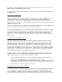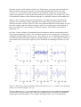
Download ULTRASONIC DECONVOLUTION TOOLBOX User Manual v1.0

ULTRASONIC DECONVOLUTION TOOLBOX
User Manual v1.0
Acknowledgment
The authors would like to acknowledge the financial support of European Commission within
the project SPIQNAR FIKS-CT-2000-00065
copyright
Tomas Olofsson
Uppsala University
Signals and Systems
July 2
CONTENTS
1.
INTRODUCTION
1
2.
INSTALLATION
1
2.1
2.2
3.
FILE FORMATS
3.1
3.2
4.
RUNNING STEPS
SOME DETAILS CONCERNING THE ALGORITHMS
5.1
5.2
5.3
5.4
5.5
6.
SUPPORTED FORMATS
ADDING NEW FORMATS
GETTING STARTED
4.1
5.
SYSTEM REQUIREMENTS
INSTALLING THE SOFTWARE
BACKGROUND TO THE DECONVOLUTION PROBLEM
DETAILS ON SATURATION HANDLING
DETAILS ON EXTRACTING THE PROTOTYPE DATA
DETAILS ON ROBUST DECONVOLUTION
DETAILS ON SEMI SPARSE DECONVOLUTION
RECOMMENDATIONS FOR ALGORITHM USE
1
1
1
1
2
2
5
9
9
12
12
13
13
14
1. INTRODUCTION
This manual presents the web release of the Ultrasonic Deconvolution Toolbox for research
pruposes (see Disclaimer). The toolbox contains the deconvolution algorithms proposed for
the SPIQNAR european project (FIKS-CT-2000-00065). The software is operated from a
graphical user interface and has been designed to be more or less self-documenting and easy
to use for NDT operators.
The software supports the MATLAB file format for reading. To read data in other formats, a
stand-alone software that converts to the MATLAB formats may be used.
The main purpose of the manual is to give a description on how to use the Deconvolution
Toolbox in practice. Mathematical details have been left out almost completely.
2. INSTALLATION
2.1 System Requirements
The Deconvolution Toolbox (DT) requires a Pentium compatible PC running Microsoft
Windows 2000, NT 4.0, 98 or ME and MATLAB 6.0 or later with the optimization toolbox
installed.1 The computer should be equipped with at least 128 MB of RAM for the software to
run smoothly.
It is assumed throughout this manual that MATLAB is properly installed and that the user is
familiar with using Microsoft Windows.
2.2 Installing the Software
The software is supplied in a zip-archive containing the required MATLAB p-files. In order
to install the software, create a new directory on the hard disk and unpack these files into the
directory. The new directory must then be added to the MATLAB path, which is done by
clicking on the Path Browser button in the MATLAB command window.
3. FILE FORMATS
3.1 Supported Formats
As distributed, the following file formats can be read using the Deconvolution Toolbox:
•
Native MATLAB (.mat). The B-scans must reside in ordinary matrices and with the
A-scans organized in columns. Four example files are distributed along with the
software so that the user has the chance to get started.
At present, no more information than the raw amplitude data is used from the files. This
means that the time will only be represented by the sample indices (integers) and not in (µs),
and the A-scan position is given as an integer instead of in (mm).
1
Most of the functionality in the Deconvolution Toolbox will still be available without having the optimization
toolbox installed. It is only the “Advanced saturation handling” that will be lost, see description below.
1
3.2 Adding New Formats
Adding new file formats can be done by the user as the file loading functions are supplied as
MATLAB source files (m-files). To do this, the user must:
•
add calls to alternative loading functions in the function file LoadBscan.m. A
number of lines (lines 80 to 86 in LoadBscan.m) have been prepared for this
purpose.
•
write the loading function. When writing this function, note that the path and the
filename of the chosen file are found in the variables pathname and filename,
respectively.
For example, to prepare for reading *.qwe-files, change the line (line 80) “elseif
filename(length(filename)-2:end)==’xxx’” to “elseif
filename(length(filename)-2:end)==’qwe’”. Then add, for instance, the line
“tempdata=GetQWEdata(pathname,filename,NoOfAscans)” and write a
corresponding function file GetQWEdata.m, that does the work. Place the new file in the
same directory as the functions in the toolbox or in a directory that is in your Matlab path.
4. GETTING STARTED
To start the Deconvolution Toolbox, first start MATLAB and then type deconvtool on the
command line. The graphical user interface will then appear. By using the graphical controls
the operator can load and view US data, perform deconvolution and save the processed data.
Prototype data (variables describing the transducer impulse response) required by the
algorithms may also be loaded or extracted from the current B-scan and saved for later use on
similar data.
After loading a B-scan, it can be viewed either in gray scale or in color. The raw B-scan data
and one A-scan are shown on the left hand side and the corresponding processed data are
shown to the right.
When loading a new B-scan, the processed B-scan will automatically be reset to zero. After
loading or extracting the prototype data, the user can choose to perform deconvolution on a
separate A-scan, the entire B-scan or a specified rectangular region in the B-scan. The newly
processed region or A-scan will be inserted at the correct position in the processed B-scan
without affecting data outside this region. This means that after a session, the processed Bscan may contain data that have been processed in different way and by using different
parameter settings. Therefore, if the processed data is to be processed further by using other
algorithms, a final processing of the entire B-scan is recommended before saving the
processed data.
Deconvolution seeks to restore a signal that has been distorted by a convolution disturbance.
In this manual this underlying signal is referred to as the reflection sequence and the
processed data is considered to consist of estimates of such reflection sequences. See Section
5 for a few more details.
2
Before describing the different controls of the toolbox, there are three features that need to be
mentioned. These features are the ones that make the algorithms in the Deconvolution
Toolbox different from standard deconvolution algorithms. The first such feature is the
possibility to perform robust deconvolution. “Robust” in this particular context means that the
algorithms are designed to be less sensitive to natural variations in the prototype waveform
that are used for the deconvolution. Apart from the prototype waveform, required by all
classical deconvolution methods, the robust deconvolution algorithms in this toolbox also
requires information that describes natural variations in the prototype waveforms. This
information is represented in the form of a covariance matrix. Below the term “prototype
data” refers to both the prototype and its associated covariance matrix.
Another feature is the so-called semi sparse deconvolution. In sparse deconvolution, the
signal is assumed to consist of only a number of “spikes” with different amplitudes. The rest
of the signal is assumed to have zero amplitude. Therefore, sparse deconvolution can be seen
much as a detection algorithm. Semi sparse deconvolution is one way of loosening this “spike
assumption”. It gives the user the possibility to gradually change the level of contrast in the
solution, from an almost completely sparse solutions as described above, to having more
evenly distributed amplitude values
Finally, the third important feature is the possibility to treat saturated data, i.e., data
containing amplitudes that have reached the “ceiling” or “floor” limits of the A/D-converter.
If the data has been acquired using an ordinary 8 bit A/D-converter, the amplitudes are limited
to the interval [-128,127] and amplitudes that were originally outside this interval will be
saturated at the lower or upper limits. Performing deconvolution on such data typically results
in artefacts. The toolbox allows for the treatment of such saturated data with only a gradual
decrease in performance.2
In Fig. 1,the graphical user interface of the Deconvolution Toolbox is shown. The objects
indicated by the numbers are described briefly in the list below. These numbers are used
throughout the manual to identify the different objects in the user interface. More detailed
descriptions on the controls are given in section 4.1.
2
Note, however, that there will almost certainly be a decrease in performance when having saturated data
instead of non-saturated data since the saturated data is less informative.
3
9
4
2
11
12
8
1
13
14
5
15
3
16
10
18
7
17
6
19
Fig. 1. The graphical user interface of the Deconvolution Toolbox.
1. A figure window for showing the original B-scan.
2. A switch between color and gray-scale presentation of the B-scan data. The original
B-scan window (1) and the processed B-scan window (8) share this color setting.
3. A figure window for showing the A-scan that is selected by means of controls (4) or
(5) seen to the right of the original B-scan. A line in the B-scan in (1) indicates the
position of the currently selected A-scan.
4. A box indicating the position of the currently selected A-scan. This integer can be
changed by activating the box with the mouse and typing in the number or by using
the slider (5).
5. A slider for selecting the A-scan.
6. A figure window for presenting the currently used prototype data. The presentation
includes error bars (defined as +/- one standard deviation) that indicate the accuracy of
the prototype. The prototype data is obtained using the controls in the Prototype data
frame (12).
7. A frame containing the controls for selecting a region in the B-scan. The data in the
selected region can later be deconvolved separately. Furthermore, the region is used
when extracting new prototype data and when estimating the noise and signal
variances (18). After pressing the “Mark” button, the user can select a rectangular area
in the original B-scan by dragging the mouse between the corners in the rectangle.
Alternatively, the corners positions can be typed in directly in the boxes.
8. A figure window for showing the processed B-scan.
4
9. A frame containing sliders for controlling brightness and contrast for the processed Bscan in (8). Note that the original B-scan in (1) is not affected by these controls.
10. A figure window for showing the processed A-scan corresponding to the A-scan
shown in (3). A line in the processed B-scan (8) indicates the position of the processed
A-scan.
11. A frame containing the controls for loading B-scans and saving processed data. Popup
menus assist both the loading and saving operations.
12. A frame containing the controls for extracting new prototype data from the current Bscan, loading this data from a file or saving prototype data to a file.
13. A frame containing the controls for starting the deconvolution calculations. By
pressing the appropriate button, the full B-scan, a region in the B-scan or a single Ascan can be deconvolved.
14. A box that shows how many A-scans that are still left to process. This helps the user to
estimate the remaining computation time.
15. A frame containing the controls for robust deconvolution. By clicking at the radio box,
the user can activate or deactivate the use of robust deconvolution. A slider helps
controlling the amount of robustness imposed on the solution
16. A frame containing the controls for semi sparse deconvolution. By clicking at the
radio box, the user can activate or deactivate sparse deconvolution. The slider is used
for controlling the contrast in the solution. The number of iterations in the iterative
algorithm can be edited in a box. This number influences the computation time.
17. A frame containing the controls for the saturation handling. The user can switch
between the simple (default) and the advanced method by clicking the radio box. The
lowest and the highest value represented by the A/D-converter are set manually in the
boxes called “lower” and “upper”, respectively. The default values are –128 and 127,
corresponding to ordinary 8 bit representation.3
18. A frame containing boxes for showing and editing the noise and reflection sequence
variances. By pressing the corresponding estimate buttons, these parameters can be
estimated using data in the selected region.
19. A button for closing the graphical user interface.
4.1
Running steps
Loading a B-scan
A session typically starts with loading a B-scan from a file. For example, to load the file
CompPlate3.mat in the directory c:\SPIQNAR\testdata\dec, follow the steps:
1. Press Load in the US data frame ( (11) in Fig. 1). The menu in Fig. 2 then appears.
3
Note that it is generally assumed that the amplitudes in the loaded data are zero mean.
5
2. Go to the directory and click on CompPlate3. Press “open”.
Fig 2. The load menu.
The loaded B-scan and the processed data (initially set to zero) should appear in (1) and (8),
respectively.
A message box informs the user about the minimum and maximum amplitudes found in the
loaded B-scan. If the data appears to have been saturated in the A/D-conversion, these values
are the limits to be set in the Saturation handling frame (17).
Note that the file CompPlate3.mat in the example above comes with the toolbox files.
You should find this, and three similar data sets in the same directory as the toolbox files. The
data sets were obtained from a layered composite material using three different transducers.
Although the data is not representative for the data in the SPIQNAR project, it is a good set in
the sense that the data is well behaved and it helps showing the potential of deconvolution
methods. It illustrates what can be done when representative prototypes and reasonably clean
data are available.
Obtaining new prototype data
If it is the first session with the toolbox, the user should extract new prototype data. This data
will consist of (i) a prototype and (ii) a corresponding covariance matrix describing the
natural variations of the prototype.4 The extraction of these two variables should be done
using the following steps:
1. Select a region containing a number of good prototype representatives. Select the
region by pressing Mark in the Region Selection frame (7) and drag the mouse in
the original B-scan (1) to mark a rectangle. Alternatively, define the rectangle by
typing the region limits directly into the boxes in the frame.
2. Press New in the Prototype data frame (12).
3. After a while a prototype appears along with its error bars in the Prototype figure
(6). The start and end positions of this prototype must first be identified before the
prototype can be used for the deconvolution. To do this, mark the start position of
4
In the code the prototype and the covariance matrix are named Prototype and Ch, respectively.
6
the prototype using the mouse. Then drag the mouse to the end position and finally
lift the mouse button. The part inside the time interval indicated by a rubber box
will be used (see Fig 3, below)
4. The prototype should now appear once again in the same figure window but now
starting at the position marked earlier by the user. This time the prototype is
presented using the same time scale as the A-scan and B-scan data.
Fig. 3. Isolating the extracted prototype in time. The rectangular box that defines the start
and end position is obtained by clicking at the start position and dragging the mouse.
Loading prototype data
If prototype data has already been extracted and saved in earlier sessions, the saved file
consists of both the prototype and its associated covariance matrix. It is then straightforward
to load the prototype data. Simply press the Load button in the Prototype data frame (12)
and open the file of interest.
If the chosen file does not contain the covariance matrix, the user can still load the impulse
response. Note that robust deconvolution cannot be performed in this case.
Saving prototype data
To save the prototype and its associated covariance matrix for later use, simply press the
Save button. A popup menu will appear and the user can choose directory and file name. The
saved file will contain the prototype in the variable Prototype and the covariance matrix in
the variable Ch. If Prototype is a columns vector of size N, then Ch will be a square N
times N matrix.
Deconvolving the data
If the B-scan and prototype data are available we can now perform the deconvolution. Note
that the algorithms require the noise and signal variance parameters (18) and the saturation
limits (17) to be set. However, these are initially set to default values that are hopefully
appropriate for the current B-scan. The steps for setting these parameters are described in
separate subsections below.
If a new prototype was extracted from the B-scan, a region has already been selected and the
Region button in the Deconvolve frame (13) should be enabled. A good starting point is
then to perform deconvolution in this region by simply pressing this Region button. If the
data is reasonably well behaved, the deconvolution should result in a series of relatively sharp
peaks at the positions of the prototypes in the selected regions. If not, try activating the robust
deconvolution in (15). (Press the Region button once again). If this solves the problem, we
now know that the solution is sensitive to small variations in the prototype and we should
7
preferably use robust solution from now on when working with this data set, or try to find a
better region for estimating the prototype data.
To perform deconvolution on the full B-scan or the selected A-scan, press the B-scan or the
A-scan button.
Setting the saturation limits
The two controls for the saturation handling are found in the Saturation handling frame (17).
The radio box with the text “simple/advanced” indicates which of the methods that is
currently active. The default is “simple”. Below the radio box there are two edit boxes. The
default values are –128 and 127. These should be the proper values when treating data having
amplitudes stored in 8 bits.
The user is informed about the minimum and maximum amplitude values when loading a new
B-scan. These two values may be the correct saturation limits to set.
The saturation handling is always active when using the Deconvolution Toolbox but it can be
deactivated in practice by setting the lower and upper saturation limits to large negative and
large positive values, respectively. By setting the limits to values smaller than the correct
limits, the user can investigate the effects of using data with amplitudes being thresholded at
different levels.
Setting the noise and signal variances
The values of the noise variance and the reflection sequence variance are shown in frame
(18). Note that “noise” here actually refer only to the measurement noise and not to any socalled material noise. If the data was acquired using waveform averaging, only very little
noise should remain from the electrical amplifiers etc and the measurement noise should
mainly consist of quantization noise that has a variance of around 0.15. In practice, setting the
noise level this low might yield very noisy results. A larger noise level is typically needed for
regularising the solution somewhat. Note, however, that when we use robust deconvolution,
much of this regularisation is automatically taken care of.
Both the variances can be set individually by typing the values in the boxes. Alternatively,
reasonable values can be found by means of an estimation procedure that uses data in the
region defined by the user. The procedure should be as follows:
1. Use the controls in the frame (7) to define a region containing measurement noise
only. Press the estimate button associated with the noise variance.
2. Select a new region that seems to be representative in terms of signal energy. Press the
estimate button for the reflection sequence. Note that this estimate is based on the
noise variance as well as the prototype waveform.
Setting parameters for robust deconvolution
To perform robust deconvolution, simply activate the radio box in the Robust deconvolution
frame (15) and press any of the deconvolution buttons. The slider called level gives the
user a possibility to gradually control the amount of robustness to natural variations in the
prototype. Placing the slider to the left means that the information in the prototype covariance
8
matrix is down-weighted when used in the algorithm. When the slider is at its leftmost
position, the influence from this covariance matrix is identically zero and the solution should
in such a case coincide with its corresponding non-robust solution.
Note that if no prototype covariance matrix is available, the robust deconvolution algorithms
can produce no results. In this case a warning is given to the user.
Setting parameters for semi sparse deconvolution
To perform semi sparse deconvolution, activate the radio box in the semi sparse
deconvolution frame (16) and press any of the deconvolution buttons. The level slider gives
the user the possibility to gradually change the contrast of the solution. For example, a high
level will typically yield solutions that contain a few, large peaks and with the remaining
amplitudes being very close to zero. Setting the level low yields a solution with more evenly
distributed amplitude values. Setting the level to the lowest possible value will have the same
effect as deactivating semi sparse deconvolution.
Semi sparse deconvolution is implemented as an iterative optimization procedure. In the
frame there is a box showing the number of iterations used by the algorithm. The default
value is 8, which has proven to be appropriate in many experiments. Since the calculation
time is approximately proportional to this number, this number should be kept as small as
possible. However, when the number is set too small, the algorithm will stop before
converging to the proper solution. To assist the user in finding a good compromise between
calculation time and convergence, the current estimate is presented at every iteration.
5. SOME DETAILS CONCERNING THE ALGORITHMS
Although most of the information that is needed for using the toolbox has now been given,
there are still a number of details that should be mentioned. Also, a number of concepts that
were mentioned only very briefly might need some additional explanation. Therefore a (still
rather brief) background to the deconvolution problem in general and the to the issues treated
in the toolbox in particular, is first given in the following subsection. The details associated
with the extraction of prototype data, saturation handling, robust deconvolution, and semi
sparse deconvolution are then presented in separate subsections.
5.1
Background to the deconvolution problem
Deconvolution deals with the problem of removing an unwanted convolutional distortion
from a signal, r(k), where the integer k is the time index. In ultrasound data, r(k) is sometimes
called the reflection sequence and it can be thought of as the signal that would be obtained
using a very broadband transducer that has a Dirac pulse (a “spike”) as its impulse response.
A common and practically relevant assumption is also that the measured signal, x(k), has
been corrupted by a measurement noise sequence, e(k). Using a convolutional signal model,
x(k) can then be written mathematically as
x(k) = h(k)*r(k) + e(k)
(1)
where * denote the convolution and where the impulse response, or the prototype, h(k),
models the convolutional distortion. When we in the manual mention the noise variance, we
9
mean the variance of the random variable e(k). Furthermore, we assume (at least implicitly)
that the samples in the noise sequence are uncorrelated and that they all have the same
variance, i.e., we assume the noise sequence to be stationary. In this way we need only a
single scalar parameter to describe the measurement noise properties. In a similar way, when
we mention the variance of the reflection sequence, we mean the variance of the sample r(k).
When we are not using semi sparse deconvolution, we (implicitly) assume the reflection
sequence to be stationary so these algorithms also require only a scalar parameter for the
reflection sequence variance. However, there is an important difference between how we treat
the noise sequence and the reflection sequence when we use semi sparse deconvolution. In
this case we allow for a non-stationary reflection sequence. The details are described in
subsection 5.5.
In Figure 2, three examples of simulated reflection sequences and the corresponding (noisefree) measured signals are shown. The reflection sequence in (a) contains only two non-zero
amplitudes and this signal is said to sparse. The sequence in (b) is completely random (here, a
so-called uncorrelated Gaussian sequence) and the sequence in (c), is an example of what we
in the manual call a semi sparse signal. It can be described as something in between (a) and
(b).
Figure 2. Illustration of three simulated reflection sequences, (a) - (c), and the corresponding
(noise free) measured signals, (d) - (f).
The convolution in eq. (1) can be thought of as a superposition of time-shifted and amplitude
scaled replicas of the prototype, h(k), where the amplitude scales are simply the amplitudes
found in the reflection sequence. For example, the signal in Fig. 2 (d), is constructed by
10
superimposing two prototypes starting at time indices k=50 and k=150, each scaled with
factors +1 and –0.5, respectively, as indicated by the corresponding reflection sequence in (a).
One of the main motives for performing deconvolution of ultrasonic signals in NDT is to
improve the time resolution. Ideally, one would like to see the signals in the upper row in Fig
2, instead of the ones in the lower row. Among other things, the presence of measurement
noise makes a perfect reconstruction impossible. Furthermore, there are a number of other
aspects that needs to be considered before being able to perform accurate deconvolution.
First, a good deconvolution result requires precise knowledge about the prototype to
compensate for. Therefore, if we have reason to believe that our prototype is of bad quality,
we should have means for guarding against this. Since, in practice, the prototype is typically
obtained by picking out a representative waveform from measurement data, prototype errors
may for instance be caused by: (i) measurement noise (ii) simply picking out a bad
representative for the current data set.
Second, we must be aware of potential signal disturbances.5 One such disturbance is the
amplitude saturation caused by the limited amplitude range of the A/D-converter. Typically
the signal amplitudes in the raw data are represented by integers between between –128 and
127. If we wish to record weak reflections without too much quantization noise, we may need
to increase the gain so much that some of the other and stronger reflection will become
saturated. This saturation introduces a nonlinearity in the formation of the measured data and
this will violate the linear signal model in eq. (1). If the saturation is not taken into account,
the deconvolution of saturated data will typically result in artefacts.
Third, since the methods for deconvolution rely on prior statistical assumptions concerning
both r(k) and e(k), we should have some flexibility when choosing how to model these.
In the toolbox there are ways of treating all three above-mentioned issues. The first one is
treated by means robust deconvolution. In robust deconvolution, the algorithms are designed
to be less sensitive to variations in the prototype. Thus, the choice of prototype should not be
as critical as it is in ordinary methods. The information about the variations of the prototype is
obtained by using several signals, instead of only one, when picking out the prototype from
the raw data. One average prototype and an associated covariance matrix are extracted using
these signals. It is the information in the covariance matrix that determines the performance of
the robust deconvolution algorithms. Setting the covariance matrix to a zero matrix is
essentially the same as saying that the prototype is known with perfect accuracy. Applying
robust deconvolution in this case gives exactly the same results as using ordinary (non-robust)
deconvolution.
The amplitude saturation problem is treated in two different ways in the toolbox. The simple
version is based on neglecting all samples with saturated amplitudes. By doing this, we will
still be able to set up a linear signal model which can be treated with relatively simple
methods. Note, however, that when we are using this simple approach we are deliberately
discarding some of the information. For example, in a case when the upper saturation limit is
127, we know that any sample that was recorded with this amplitude originally had amplitude
larger than or equal to 127. This information, although being less precise than the
information in a non-saturated amplitude, can be added as a constraint when seeking a
5
That is, disturbances apart from the measurement noise, e(k), which is usually handled in an fairly optimal way
in most standard deconvolution algorithms
11
solution that matches well to the data. This latter approach is used in the toolbox where it goes
under the name Advanced Saturation handling.
Finally, the toolbox allows for some flexibility when it comes to representing the user’s prior
knowledge about the reflection sequence. For example, the user might from the beginning
assume that only a few of the samples in the reflection sequence have strong amplitudes and
the remaining amplitudes are being close to zero. This will be true when there is only a small
amount of grain scattering and a small number of strong reflectors in the object. One
disadvantage of using the ordinary Wiener filter on such data is that the amplitudes of large
peaks in the signal are typically underestimated. Furthermore, the peaks are also surrounded
by “ringing”, something which may mask other nearby peaks. Methods for sparse
deconvolution seek to solve this problem by performing more or less a combined detection
and estimation procedure. As an alternative, the method of semi sparse deconvolution that is
used in the toolbox allows the user to set a level of contrast where the highest level will yield
solutions that should be very similar to those obtained by sparse deconvolution methods and
the lowest value will yield exactly the same results as those obtained by Wiener filtering.
5.2
Details on Saturation handling
The saturation limits play roles not only when performing the deconvolution but also when
the prototype data is extracted from a region in the B-scan. Since deconvolution using a
prototype that has been saturated typically yields results with very strong artefacts, the
extraction of the prototype uses the saturation limits for detecting such bad quality prototypes
and, if possible, repairs these by means of an interpolation technique. Note that if the limits
are mistakenly set too low, the interpolation is set to work without reason and we will obtain
worse prototype estimates than is necessary.
When using the saturation handling on well behaved data sets and having good estimates of
the prototypes etc., the advanced method will typically yield better results than the simple
method but at the cost of an increased computation time. However, the advanced method
seems to be somewhat less robust than the simple method when it comes to bad quality data.
At present, we do not have a good explanation for this but it is likely that it is has something
to do with imposing “hard” constraints on the solution in a situation where some of the used
parameters are known only to a very limited accuracy. The simple method only imposes
“soft” constraints.
5.3
Details on extracting the prototype data
When pressing the New button in the Prototype data frame, the data in the selected region is
used for extracting (i) a new prototype and (ii) a corresponding covariance matrix describing
the variations among the prototypes in data set. The extraction of the mean prototype and the
covariance matrix proceeds in the following steps:
• If there are signals that have been saturated by the A/D-converter, a routine that fill in
the missing values by means of interpolation is activated. This routine will not
perform the interpolation on signals that have been heavily saturated since then there
will most likely not be enough data for obtaining good interpolation values. Such
heavily saturated signals are therefore usually discarded. The interpolation is based on
simply matching a second order polynomial to a number of the data points at each side
of the missing data points.
12
•
•
•
•
•
•
The signals that were not discarded in the interpolation step mentioned above are
aligned in time using a correlation technique.
The signals are normalized and the normalization constants for each signal are
temporarily stored.
The mean and the covariance matrix of the normalized signals are calculated.
The mean is brought back to its original norm using the stored normalization
constants. The so obtained signal will be stored in the variable Prototype,
The covariance matrix is also rescaled using the normalization constants.
The obtained mean prototype plus/minus one standard deviation is plotted in the lower
left window. Irrelevant signal parts that comes from selecting too large a region can
now be removed by graphically specifying the start and the end position of the
prototype as described in Section 4.
5.4
Details on Robust deconvolution
In classical deconvolution methods such as the Wiener filter, robustness to errors in the
prototype can be obtained by increasing the noise variance. However, this is usually not a
good way to treat the problem. The presence of model errors can actually be introduced to the
signal model by adding an extra noise term. This added noise term differs from the usual
measurement noise term in the sense that it is highly colored, i.e., it has an associated power
spectrum with high peaks as well as large frequency regions where the spectrum is almost
zero. By simply increasing the noise variance, we destroy information in all frequency to an
equal extent; thus, we may destroy information in frequency bands that are not particularly
affected by the model error. The robust deconvolution methods implemented in the toolbox
are designed to treat this problem optimally.
Essentially, there is no need for user parameters when working with robust deconvolution
algorithms. All necessary information is kept in the prototype covariance matrix that is
extracted using a region in the raw data. However, a slider still gives the user the possibility to
choose how much the covariance matrix will influence the solution. This option should
perhaps be excluded in a final implementation but can be of interest in a first version. Note
that the default slider setting (that is, in its middle position) corresponds to using the prototype
data in the theoretically proper way. Setting it to zero (leftmost position) corresponds to the
situation of not using the information in the covariance matrix at all.
5.5
Details on Semi sparse deconvolution
The algorithms for semi sparse deconvolution are different from the other algorithms in the
important aspect that the reflection sequence is allowed to be non-stationary. This is
implemented in the algorithms by having a sequence of variances (one variance6 for each
sample in the reflection sequence) instead of a single scalar variance for all samples.
The algorithms then iteratively modify this sequence of variances to better match to the data.
The algorithm starts from setting all variances in the variance sequence to the same number.
This number is the parameter that can be set by the user in the box in the “Noise and Signal
variance” frame. The iteration proceeds by calculating the reflection sequence estimates based
on the variances in the sequence, then redistributing these variances so that the ones
6
Actually, the variances are represented in the code by the corresponding standard deviations (the square root of
the variances) since this turns out to be more convenient.
13
corresponding to large amplitudes in the reflection sequence are set to high values and vice
versa. The procedure is iterated a number of times.
The redistribution of variances is made in a controlled fashion by constraining the solution so
that the sum of variances in the sequence is kept constant. Furthermore, the sum of the
inverses of the variances is also constrained to be constant. By changing this second constant,
the “contrast” in the solution can be controlled. Setting the constant to a large value
essentially means that we allow some of the variances to be very small, which in turn will
cause their corresponding reflection sequence amplitudes to be small. As a consequence, to
meet the first constraint, some of the other variances need to be increased. By lowering the
constant, the difference between the lowest and highest possible variance is reduced and at a
certain level, the constraints will “meet on the middle” and force the variance sequence to be
the same for all samples. The constrained optimization problem associated with sparse
deconvolution is implemented using the technique of Lagrange multipliers.
6. RECOMMENDATIONS FOR ALGORITHM USE
The toolbox has been implemented in a way that essentially all variants of parameter settings
are possible. It is difficult to give recommendations that cover all possible combinations. In
the following only the main observations from working with the algorithms are listed.
•
Robust deconvolution seems to be meaningful tool and is recommended when
working with most data. Finding good prototypes is a difficult problem and the
robust method seems to handle this problem in a good way.
•
If possible, use a separate data set for extracting the prototype data. From a
deconvolution perspective, the prototype data can almost be said to be more
important for the final result than the test object data itself.
•
Semi sparse deconvolution is generally less robust than ordinary deconvolution
methods. If the intended use is to simply extract a number of the highest peaks, it is
recommended that the noise variance be raised considerably. This will turn the
algorithm more into a detector than a deconvolution algorithm.
•
The simple saturation handling is recommended in most situations. First, it is faster
than the advanced version. The simple method actually gets faster as the number of
saturated samples increases (less data is processed). The opposite holds for the
advanced method. It is only for rather well behaved data that the advanced method
offers any significant advantage over the simple version. When the number of
saturated samples is small, the two methods yield almost identical results.
14