Download Times User Manual - Department of Information Technology

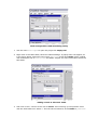
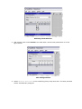
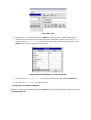
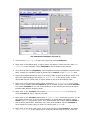
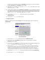
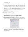
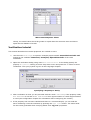
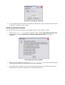
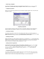
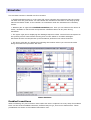
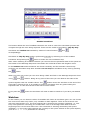
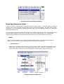
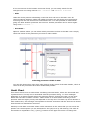
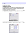
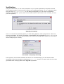
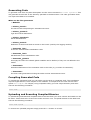
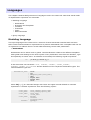
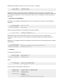
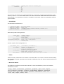
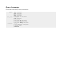
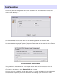
The
TIMES Tool
version 1.0 beta
User Manual
Introduction
TIMES is a modelling and schedulability analysis tool for embedded real-time systems, developed
at Uppsala University. It is appropriate for systems that can be described as a set of preemptive
or non-preemptive tasks which are triggered periodically or sporadically by time or external
events. It provides a graphical interface for editing and simulation, and an engine for
schedulability analysis.
The main features of TIMES are:
A graphical editor for timed automata extended with tasks, which allows the user to model
a system and the abstract behaviour of its environment In addition the user may specify a set
of preemptive or non-preemtive tasks with parameters such as (relative) deadline, execution
time, priority, etc.
z
A simulator, in which the user can validate the dynamic behaviour of the system and see
how the tasks execute according to the task parameters and a given scheduling policy. The
simulator shows a graphical representation of the generated trace showing the time points
when the tasks are released, invoked, suspended, resumed, and completed.
z
z A verifier for schedulability analysis, which is used to check if all reachable states of the
complete system are schedulable that is, all task instances meet their deadlines. A symbolic
algorithm has been developed based on the DBM techniques and implemented based on the
verifier of the UPPAAL tool.
z A code generator for automatic synthesis of C-code on brickOS platform from the model. If
the automata model is schedulable according to the schedulability analyser the execution of
the generated code will meet all the timing constraints specified in the model and the tasks.
More information about TIMES can be found on the web site www.timestool.com.
Installation
Before installing TIMES tool uninstall any previously installed version first. In order to do that
execute Uninstall_Timestool script from ~/Times Directory/UninstallerData directory on *NIX
systems or perform the standard uninstallation procedure using the Control Panel on Windows.
System requirements
Hardware:
CPU Pentium 166 MHz or faster or
Sparc processor
RAM 32 MB (128 MB recommended)
HDD 10 MB of available space
800x600 or higher-resolution monitor
Mouse or other pointing device
Operating system:
Linux (kernel >= 2.2.12)
Solaris 7/8/9
Microsoft Windows 95/98/NT/2000/XP
Software:
JDK 1.4.1 or higher version
PostScript Printer Driver
In order to run the Server part of the TIMES tool on a remote host you must also install and
configure an applicable network. See Installing a remote server for further information.
Installation procedure
z
Installing TIMES tool on Linux and Solaris
After downloading an appropriate for your OS timestool-1.0b.bin.gz file execute the
following commands in the directory where you have saved it and follow the installation
steps.
bash$ gunzip timestool-1.0b.bin.gz
bash$ sh ./timestool-1.0b.bin
The second screen of the wizard contains the License Agreement. Please, read it carefully and
continue the installation only if you can accept it. Choose the directory where you would like
to install the TIMES tool and the location where the links are to be put. After installation
execute the following command from your links directory to run the TIMES tool:
bash$ ./runTimestool
z
Installing TIMES tool on Windows
After downloading double-click on timestool-1.0b.exe and follow the steps of the standard
installation wizard. The second screen of the installation wizard contains the License
Agreement. Please, read it carefully and continue the installation only if you can accept it.
Choose the folder where you would like to install the TIMES tool and the location where the
icons are to be put. After installation click on the corresponding icon to run the TIMES tool.
z
Troobleshooting
If you are experiencing problems running the TIMES tool, try to execute the following
command from the directory where you have installed it:
java -jar timestool.jar
and, please, e-mail the problem description to [email protected]. We will fix it in the next
release if possible.
Installing a remote server
The TIMES tool consists of two parts: the Graphical User Interface (GUI) and the Server. Thus it
can be used as either a standalone or distributed application. Since the server requires much
more computational power that GUI, one might want to run it on a powerful remote host.
Moreover running the server separately allows several users to use it simultaneously. Currently
only Linux based systems can be used for hosting the TIMES tool server.
In order to use TIMES server remotely you have to configure it to run as a network service. Create
a service configuration file in /etc/xinetd.d/timesserver with the following contents:
service timesserver
{
disable = no
socket_type
protocol
wait
user
passenv
server
flags
}
=
=
=
=
=
=
=
stream
tcp
no
root
PATH
/path/to/the/times/server/server
NODELAY
Add the following two lines to your /etc/services file:
timesserver
timesserver
2351/tcp
2351/udp
This will setup the TIMES server run on the port number 2351. You can specify the number of any
available port here but ensure you have your clients configured appropriately.
Execute the following command in order to restart xinet daemon:
bash$ /etc/init.d/xinetd restart
You are ready to use your Linux box as a remote TIMES server! Don't forget to configure your
TIMES clients to use the remote server (see Configuration for further information).
Tutorials
The tutorials show in a step-by-step manner how the different parts of the TIMES tool work
allowing you to start quickly using the tool in your own projects.
z
z
z
z
z
Editing tutorial
Simulation tutorial
Schedulability analysis tutorial
Verification tutorial
Code synthesis tutorial
Editing tutorial
This tutoral describes how to create a very simple system using the TIMES editor. It will help you
understand the main concepts of the editor.
z
Creating an empty project
Abstract: Create a new project, name it Simple, and then save the project to the file named
empty.xml.
1. Start the TIMES tool or, if you have it already started, save and close the current project
and create a new one using menu File->New.
2. Double click the edit box of the project attribute Name. The current name Project will
be highlighted. Type in the new project name Simple.
3. Use the menu File->Save As... to save your project. A standard file dialog will
appear. Type in the filename empty, and click the Save button.
4. Use the menu File->Exit to close the tool.
z
Adding and configuring tasks
Abstract: Create two tasks as shown in the figure below and then set the deadline monotonic
scheduling policy. Set the maximum of 2 task instances for the task1 and save the project as
tasks.xml.
Task Configurations and Scheduling Policy
1. Use the menu File->Open to open the project file empty.xml.
2. Right-click in the tasks table, below the table headings. A popup menu will appear, as
in the figure below. Select the menu item Add task. A new task task1 will be created
with its behavior set to controlled. See Editor chapter for more information about the
task table.
Adding a Task to The Task Table
3. Left-click in the B column of the row for task1. This will bring up a drop-down menu
with the task behaviors. Select P. This will set the behavior of the task1 to prediodic.
Selecting Task Behavior
4. Add another task named task2 to the task table. Set the task parameters as in the
figure below.
Task Configurations
5. Select Deadline Monotonic in the scheduling policy drop-down box. The task priorities
will be automatically assigned.
The Tasks Tab
6. Select the Tasks tab and then select task1 in the task table. The attributes of the
selected task will appear in the panel below the task table. Double-click in the value
column of the Max # of tasks row and type in 2. This will allow two instances of the
task1 to be active at any time as maximum.
Setting Maximum Number of Task Instances
7. Use the menu File->Save As... to save the project to the file named tasks.xml.
8. Use the menu File->Exit to close the tool.
z
Creating an automaton template
Abstract: Create an automaton template p(const T), as in the figure below. Save the project
as automaton.xml.
The automaton template 'p(const T)'
1. Use the menu File->Open to open the project file named tasks.xml.
2. Right-click in the tabbed area. A popup menu will appear, select the menu item Add
template. A new template, called Template1, will be added to the project.
3. Go to the tab with the Template1. The template properties will appear below the task
table. Change the template name to p and type in const T in the Parameters field.
4. Below the template attributes there is an empty table of local declarations. Right-click
below the table headings and select Add declaration in the popup menu. A clock
named x1 with the initial value 0 will be added to the local declarations table.
5. Right-click in the template drawing area, and select Create->Location in the popup
menu. A new location named Location 1 will be created. Double-click below Location
1 to create Location 2. You can move locations on the drawing are as well as adjust
location label position dragging them.
6. Right-click on the Location 1 and select Location->Make initial in the pop-up
menu. Location 1 will be marked as initial.
7. Right-click on the Location 2 and select Arguments->Edit in the pop-up menu (or you
can simply double click on the location instead). An inline editor will appear. Select
task2 in the Task drop-down menu. This will associate the location with the task2 so
that it will be released for execution every time an automaton reaches Location 2.
Click outside the inline editor to close it or simply press Enter key.
8. Right-click on the blue cross (port) on the lower border of the Location 1 and select
Create transition in the popup menu (or simply double-click the port). Drag the
transition end to the upper port of the Location2 and left-click on it once. A transition
between Location1 and Location2 will be created.
9. Right-click on the transition line and select Arguments->Edit in the popup menu. Type
in x1 >= T in the Guard field.
10. Create another transition, from Location 2 to Location 1. During dragging a transition
end create two nails (turning points) in order to bend the transition line by left-clicking
on the drawing area at their locations. Right-click on the newly created transition and
select Arguments->Edit. Type in x1 := 0 in the Assign field.
11. Use the menu File->Save As... to save the project in the file named
automaton.xml.
12. Use the menu File->Exit to close the tool.
z
Creating a process
Abstract: Create a process named Process 1 as in the figure below. Save the project as
process.xml.
Your First Process
1. Use the menu File->Open to open the project file automaton.xml.
2. Click on the project tab Simple and double-click in its drawing area. A process
Process1 will be created.
3. Double-click on the Process 1 to open an inline editor. Select template named p in the
Template drop-down menu and type in 7 in the Parameters field.
4. Use the menu Run->Syntax checking to run system syntax checking procedure. A
message should appear saying that the system is syntactically correct. If not, check
whether you have performed all the steps as described in this tutorial. The error
message dialog will describe the errors you have made and help you to locate them.
5. Use the menu File->Save As... to save the project to the file named process.xml.
6. Use the menu File->Exit to close the tool.
Simulation tutorial
This tutorial describes how a system is simulated in the TIMES simulator.
1. Use the menu File->Open to open an example project named Controlled+Periodic.xml
located in the subfolder Timestool/ examples/ SporadicPeriodic of the TIMES
installation.
2. Start the TIMES simulator using the menu Run->Simulator.
The TIMES Simulator
3. Simulation in step-by-step mode is performed manually. Select one of the enabled
transitions and press the
button to make one simulation step.
Note: When selecting an enabled transition you can see the next predicted system state at
the bottom of the Message Sequence Chart below the violet bar drawn with lighter colors.
4. The random run simulation mode is activated by pressing the
button. In this mode
transitions are chosen randomly and the simulator continuously performs one simulation
step after another. To stop simulation press the
button.
5. You can reset the simulatior to its initial state pressing the
button. When there is a
trace in the Message Sequence Chart you can move along it back and forth, observing the
system internal state and variable values in all simulator views, using
and
buttons. The
button sets the simulator to the end of the trace from where you can
continue current simulation.
Note: If you continue simulation somewhere from the middle of the existing trace, the tail
of this trace will be erased.
6. You can also navigate along the trace by clicking either on the Message Sequence Chart
levels or on the Gantt Chart time points.
7. In the Message Sequence Chart process states are hidden (replaced by a thin vertical line)
if they have the same names as the name of a state since the last state change. To view
the state names of all processes at a certain level of the chart move over the pointer to this
level.
8. You can switch back to the editor view preserving the state of the simulator by using the
menu Window->Editor. In order to return to the simulation use menu Window->Simulator.
Note: If you rerun the simulator from the editor via menu Run->Simulation, the state of
previous simulation will be reset and the system being edited will be uploaded to the
simulator again.
9. You can close the simulator using menu File->Close Simulator.
Schedulability analysis tutorial
This tutorial describes how the schedulability analysis is performed in TIMES.
1. Use the menu File->Open to open a project to be analysed named
Controlled+Periodic.xml located in the subfolder Timestool/ examples/
SporadicPeriodic of the TIMES installation.
2. Start the schedulability analysis using menu Run->Schedulability Analysis. A new
window will pop up showing location of the server being used and an activity indicator. An
answer SATISFIED or NOT SATISFIED is returned by the time analysis has been performed.
Result of Schedulability Analysis
3. In our case the answer is SATISFIED, which means that all the tasks in the system
managed to meet their deadlines in all possible execution traces. In this case one can
observe worst-case response time of each task, i.e. the lowest integer value greater or
equal to the longest response time of a task. Press Show WCRT button to open a window
containing those values.
Worst Case Response Times
Clearly, the WCRT value should be greater or equal than the execution time and less or
equal the the deadline of a task.
Verification tutorial
This tutorial describes how model properties are verified in TIMES.
1. Use the menu File->Open to open an example project named Controlled+Periodic.xml
located in the subfolder Timestool/ examples/ SporadicPeriodic of the TIMES
installation.
2. Open the verification dialog using menu Run->Verification. In the dialog specify the
property E<>(aver>5) secting it from a drop-down menu and press the OK button to start
verification. The query syntax is given in the Languages chapter.
Specifying a Property to Verify
3. After verification is done you are provided with the result: SATISFIED, if the property holds,
NOT SATISFIED if not and MAYBE SATISFIED if Over Approximation or Under Approximation
is used (see Configuration chapter for information about configuring the verifier).
4. If the property has not been satisfied and there is a counterexample, you can load the
trace containing it into the simulator by pressing the Show trace button. The same holds
for the traces generated while verifying "E<>" and "A[] not" properties.
The Result of Property Checking
5. You can start several verification processes simultaneously. Every verification process uses
a separate connection to the verifier.
Code synthesis tutorial
This tutorial shows how to synthesise executable code from your models in TIMES.
1. Use the menu File->Open to open an example project named Controlled+Periodic.xml
located in the subfolder Timestool/ examples/ SporadicPeriodic of the TIMES
installation.
Generating Code from a Model
2. Start the code generation using menu Run->Code synthesis. In the newly opened window
you can see the names of the files that have been generated.
3. See Configuration chapter for more information about setting up the code generator and
Synthesis to learn how to compile and run the generated code.
Editor
Concepts
z
Task
A task is a piece of code, as in general real-time scheduling theory. It has properties such as
worst case execution time, deadline, and possibly others. The task behavior defines how a
task is released: periodically with the fixed period, by entering a control automaton state or
periodically with the given minimal inter-arrival time (sporadically).
z
Automaton Template
An automaton template is an uninstantiated timed automaton with tasks and possibly some
parameters. States can be associated with tasks and have invariants whereas transitions
have guards, synchronization and assignments as arguments. More information about timed
automata with tasks can be found in the paper "Timed Automata with Asynchronous
Processes: Schedulability and Decidability" on the TIMES publications page.
z
Process
A process is a building block of the system, an automaton template instantiated with the
given arguments. When the process instance enters a state with a task assotiated, an
instance of that task is released for execution.
Overview of the TIMES editor
z
Tabbed Area
We refer to the large area to the right as the tabbed area. At the top of the tabbed area there
are tabs: the project tab, the tasks tab and the template tabs, one for each defined
automaton template.
z
Task Table
The task table contains information about tasks in the system being modelled. Tasks can be
added or removed from the task table, and their parameters can be changed also. The
scheduling policy is selected from a corresponding combobox on the top of the task table.
The Task Table
There are three possible selections for the scheduling policy:
Deadline Monotonic
Task priorities are assigned according to deadlines, with the higher priority for the
shorter deadline.
Rate Monotonic
Task priorities are assigned according to periods, with the higher priority for the shorter
period.
User-defined Priorities
Task priorities are manually set.
You can add a task to the task table by right-clicking below the table heading. A popup menu
appears, select Add task and a new task will be added. Remove a task by right-clicking on a
line containing task, and select Remove task(s) in the menu.
The task parameters that can be edited directly in the task table are:
Name
The task name.
B (Behavior)
The behavior of a task, indicating how the task instances are released. The possible
values are C for controlled, P for periodic, and S for sporadic. The release of a controlled
task is specified by an automaton, periodic tasks are released periodically with the
period specified in the column T, sporadic tasks are released quasi periodically with the
minimum inter-arrival time specified in the column T.
P (Priority)
The priority of the task (bigger numbers correspond to higher priorities).
C (Execution time)
Time required for a task to complete its execution in a worst case.
D (Deadline)
Task execution deadline.
T (Period)
Period (time interval between releases of two sequential task instances) for periodic
tasks and minimal inter-arrival time for sporadic tasks.
z
Properties or Attributes
In the lower left part of the main window there is a property panel. The contents of this panel
is changed depending on the currently selected tab in the tab area. If the project tab is
selected, there is an edit box for the project name, and a global declarations table. If the
tasks tab is selected, and a task is selected in the task table, there is a table with all the task
parameters. If a template tab is selected, there are edit boxes for the template name and
parameters, a check-box showing whether the template represents environment, and a local
declarations table.
Project tab
When the project tab is selected, you can create and edit system processes and add comments in
the project drawing area.
z
Creating a process
To create a new process right-click on the drawing area where you want the process symbol
to appear, and select Create->Process in the popup menu.
Creating a process
You can also create a process by double-clicking on the empty part of the drawing area.
z
Editing process arguments
To modify process arguments double-click on the process, or right-click on it and select
Arguments->Edit in the popup menu. An inline editor will appear containing the following
fields: Name, Template, and Parameters.
Editing process arguments
The Name field contains the name of an instantiated template automaton specified in the
Template field. If you have already created templates before, simply choose the name of a
template in a combobox. The Parameters field contains actual parameter list being passed to
the template during process instantiation.
z
Creating a comment
Comments improve readability of your models. To create a comment right-click on the
drawing area where you want the comment to appear, and in the popup menu select Create>Comment.
z
Editing a comment
Double-click on the comment, or right-click and select Arguments->Edit in the popup menu
to start modifying comment text.
All the graphical elements that are created in the drawing area have additional formatting
attributes such as colors, font styles etc. that can also be modified in order to make your model
layout look nicer. This also applies to all the drawing areas described below.
Tasks tab
The major part of a tasks tab contains the task code editor. It supports customizable syntax
highlightning for the C-style program text. The task code put in this editor is used by the code
generator during creation of an executable program out of your model. The pointer to the file
containing a piece of code representing a task is specified in the corresponding field above the
editor.
There is also task interface field, where an expression should be entered showing how the task
code influence internal model variables by the end of it's execution.
When the tasks tab is selected you can also view and edit task attributes in the Attributes panel,
by selecting a task in the task table.
Template tab
Template tabs contain automata graphical editors similar to the project graphical editor. Use
those to create and modify timed automata of particular templates. As any other state chart
template automaton consists of locations (states) and transitions between them. For your
convenience there is also possible to add connectors and comments.
z
Adding a template
To create a new automaton template, right-click on the tab area, and select Add template in
the popup menu.
Adding a new template
z
Removing a template
To remove a template, right-click on a template tab, and select Remove template in the
popup menu. A confirmation dialog will appear. Choose "Yes" to remove a template.
z
Template properties
Below the task table the properties of the automaton template appear when a tab with that
template is active.
Template properties
Use the properties panel to modify the name of a template, define its formal parameters,
specify whether the template is a part of an environment and declare local variables.
z
Creating a location
To create a new location right-click on the drawing area where you want the location to
appear, and select Create->Location in the popup menu. Another way to do this is to simply
double-click on a drawing area where you want the location to be created.
z
Deleting a location
Select the location you want to delete, right-click on it, and select Delete in the popup menu.
Another way to do this is to select the location and press the DEL key. You can also select and
delete a group of locations at a time. To select a group drag a frame with your pointing
device or left-click on locations while holding the CTRL key.
z
Editing location arguments
To edit location arguments right-click on the location, and select Arguments->Edit in the
popup menu. An inline editor will appear containing the following fields: Name, Task, and
Invariant. The Name field contains location name, in the Task field a name of the task
associated with this location is specified (if any), and the Invariant field conatins an
invariant expression.
z
Creating a transition
To create a transition between locations right-click on one of the ports (blue cross on the
location border) of the source location, and select Create transition in the popup menu.
Another way to do that is by simply double-clicking on a source location port.
Creating a new transition
Move the pointer to the destination location port left-clicking at the positions where you want
to put nails (turning points) and finally left-click on a destination port. The transition creation
process will be automatically terminated. Every transition should begin and end at a location
port. To create a self-loop use the same or different ports of the same location. You can also
reconnect transitions to different locations after creating them by selecting and dragging edge
nails. Note that a disconnected transition is drawn with the red color.
z
Deleting a transition
To delete a transition select it first, right-click on it, and select Delete in the popup menu.
Another way to do this is to select the transition and press the DEL key.
z
Editing transition arguments
To edit transition arguments right-click on the transition, and in the popup menu select
Arguments->Edit. An inline editor will appear containing the following fields: Name, Guard,
Sync, and Assign. The Name field contains transition name. Guard is an expression that has to
be satisfied in order to take this transition. Sync is the name and direction of a
synchronization channel. Use a combobox to choose between one of the declared channels.
The Assign field is used to specify assignments that are performed if the transition is taken.
z
Creating a connector
To create a connector right-click on the drawing area where you want the connector to
appear, and select Create->Connector in the popup menu. Connector is a piece of
syntactical sugar since semantically connector it is a committed location that should be
passed in zero time only if both incoming and one of outgoing transitions are enabled.
z
Deleting a connector
Select the connector you want to delete, right-click on it, and select Delete in the popup
menu. Another way to do this is to select the connector and press the DEL key.
z
Comments
Comment operations are the same as in the project editor.
z
Adding a nail
Right-click on a transition in a place where you want to add a new nail, and select Add nail
in the popup menu.
z
Removing a nail
Select a nail, right-click on it, and select Remove nail in the popup menu.
Removing transition nail
TIMES menus
z
File
{
New
Create a new project.
{
Open...
Open a project file.
{
Save
Save the active project file.
{
Save As...
Save the active project to a file specified using a standard file dialog box.
{
Export to...
Export the model to either Uppaal .ta file or printable postscript document.
{
Print...
Print the grahical parts of the projects.
{
Close
Close the active project windows.
{
previously opened files
Opens a previously opened project.
{
Exit
Exit from the TIMES tool.
z
Run
{
Syntax checking
Perform a syntax check of a project.
{
Simulation
Start the simulator, as described in the simulator chapter.
{
Schedulability analysis
Start the schedulability analysis.
{
Verification
Verify a property of a model as described in the analysis chapter.
{
Code synthesis
Generate the source code for the active project, as described in the code synthesis
chapter.
{
Compile
Compile the source code generated by a code generator.
z
Options
{
Configuration...
Modify the global settings of the TIMES tool as described in configuration chapter.
z
Window
{
Editor
Show the editor window.
{
Simulator
Show the simulator window (if the simulator has been started).
{
Response times
Show the window with the worst case response times of tasks evaluated during
schedulability analysis.
z
Help
{
About...
Display a dialog box with the program version, build and copyright notice.
Simulator
The simulator window is divided into four sections:
Enabled transitions part is in the upper left corner showing the transitions that the system
can take from the given state. You can choose the transition to be taken in the step-by-step
manual simulation mode. In the random run simulation mode the transitions are randomly
chosen.
z
z Watches part is right below Enabled transitions part. Here you can observe the values of
clocks, variables as well as task and processor utilization factors at any time during
simulation.
z The upper right part is displaying the Message Sequence Chart. Vertical lines correspond to
the system process control flows showing their current states in rounded rectangles.
Horizontal arrows are interprocess synchronizations performed via named channels.
The lower right part is a Gantt Chart showing the timeline where you can see the tasks
being executed and a processor idle time.
z
Times Simulator
Enabled transitions
When simulating only one execution trace within the tree is explored. On every step of simulation
there can be several enabled transitions, different ways to go, due to non-determinism. These
possibilities are shown in the Enabled Transitions view.
Enabled transitions
The buttons below the list of enabled transitions are used to control the simulation process and
navigate through the trace being explored. There are two modes of simulation: step-by-step
simulation and random run initiated by means of control buttons
correspondingly.
and
Simulation in step-by-step mode is performed manually by selecting one of the enabled
transitions and pressing the
button to make the next simulation step.
Note: When selecting an enabled transition you can see the next predicted state of the system at
the bottom of the Message Sequence Chart below the violet bar drawn with brighter colors.
In the random run mode transitions are chosen randomly and the simulator continuously
performs one simulation step after another. You can stop the simulation at any time by pressing
the
button.
When you have got a trace you can move along it back and forth in the Message Sequence Chart
using
and
buttons. Being at any point of the trace you can observe the state of the
system together with the variable values. The
button moves the simulator to the end of the
trace that is exlored so far. It is possible to continue simulation from any point withing the
explored trace. In this case the tail of this trace will be erased.
If you press the
it.
button the simulator will reset its state to initial as if you have just started
Watches
In this section you can observe values of variables and clocks as simulation goes. You can choose
the view to see either only clocks, only variables or both together. There is also a fourth view
with two progress bars in it. The first progress bar is showing the processor utilization, i.e. how
busy is the processor executing your model tasks. This is an average value taken from the
beginning of the current execution trace. The second bar is showing momentary task queue
utilization, i.e. how many task instances are currently in the queue relative to the queue capacity
(sum of Max # of tasks parameter for all tasks).
Processor and task queue utilization
Message Sequence Chart
Traces in TIMES are represented by Message Sequence Chart (MSC), a UML-like sequence diagram
showing concurrent execution of processes and their intercommunication. The MSC view is quite
interactive: you can observe the whole execution trace, move to particular states in it, hide/show
different processes etc.
In the Message Sequence Chart process states are hidden (replaced by a thin vertical line) if they
have the same names as the name of a state since the last state change. To view the state
names of all processes at a certain level of the chart move over the pointer to this level.
z
Menus
If you move the pointer over a process name in MSC header, it will become high-lighted.
Right-click on it and a menu containing the following items will appear.
{
Find location...
Allows you to find the next occurrence of the location name of the selected process in the
whole trace. If location is found the MSC cursor (violer bar) jumps to it. Otherwise if the
end of the trace is reached you will be asked to continue search from its beginning.
Finding location in MSC trace
If one occurrence of the location name was found, you can easily search for the
next/previous one using menues Next 'location' and Previous 'location'.
{
Hide
Hides the whole process substituting it with the thick red line in the MSC view. All
communications between visible and hidden processes are still shown as outgoing and
incoming into the red vertical line horizontal arrows. It is also possible to hide several
going one after another processes into one line. Hidden processes can be shown again
using menu Processes....
{
Processes...
Opens a window where you can select which processes to show in the MSC view. Simply
check the boxes of the processes you want to make visible.
Selecting processes visible in MSC
You can also access this menu item right-clicking at any point of the MSC header, which is
useful if all the processes have been accidentially hidden.
Gantt Chart
This section has a form of Gantt Chart visualizing executed tasks, where the horizontal axis
represents time. The top line is associated with the processor idling, i.e. blue rectanges
appearing on it denote periods when the processor doesn't execute any task. On the lines
below the execution of tasks is drawn. Tasks sorted on a Gantt Chart according to their
priorities with the higher priority task depicted on the top line. The black up-arrow denotes a
task release time, red rectangle corresponds to the task execution and the down-arrow shows
that the task has finished its execution.
Similarly to the MSC view Gantt Chart is also interactive in the sense that you can move the
pointer over the timepoint you are interested in and jump to it by left-clicking. The scale of
the timeline is adjustable. Use [+] and [-] buttons in the upper left corner to change the
scale.
Simulator menus
{
File
„
Close simulator
This closes the simulator. If you just want to switch view to the editor, you should use
menu Window->Editor.
{
Run
„
Syntax checking
Performs a check of system syntax.
„
Simulation
Starts the simulator, as described in the simulator section.
„
Schedulability analysis
Determines whether the system is schedulable.
„
Verification
Displays a dialog box where you can enter the system property to be verified, as
described in the analysis section.
„
Code synthesis
Generates source code, as described in the code synthesis section.
„
Compile
Compiles generated code, as described in the code synthesis section.
{
Options
„
Configuration...
Shows the configuration dialog box, as desribed in the configuration section.
{
Window
„
Editor
Shows the editor window.
„
Simulator
This option is not available in the simulator view.
„
Response times
Shows the window with the response times resulting from the schedulability analysis.
{
Help
„
About...
Displays the dialog box with the version, copyright notice, and a web address of the
tool home Page.
Analysis
The TIMES tool supports two kinds of analysis: schedulability analysis and verification of properties
specified by temporal formulas.
Schedulability analysis
The schedulability analysis in TIMES tool is based on the reachability analysis of the scheduler
automaton that is constructed according to the chosen scheduling policy. An automaton is
schedulable if there exists a (preemptive or non-preemptive) scheduling strategy such that all
possible sequences of events accepted by the automaton are schedulable in the sense that all
associated tasks can be computed within their deadlines.
To run the Schedulability analysis select the menu item Run->Schedulability analysis. When
the computation is finished the property schedulability is shown to be SATISFIED or NOT
SATISFIED.
Schedulability Property is SATISFIED
Once schedulability analysis has been performed and the result is positive you can observe the
Worst Case Response Times (WCRT) of the tasks in the system. Click on the Show WCRT button or
use menu Window->Response times to open a window showing worst case response times.
Worst Case Response Times
Verification
Using the verification you can check properties of your system specified by temporal formulas.
The complete syntax of the formulas is given in the Languages chapter. To run verification select
the menu item Run->Verification. In the dialog that appears you can select a predefined
property (read from the .q file, which has the same name as the name of the .xml file), or write
your own property.
Entering a Property
Click OK to check the specified property. A result dialog appears, with a progress bar. When the
progress completes, the result is displayed as SATISFIED, NOT SATISFIED or MAYBE SATISFIED if
Over Approximation or Under Approximation was used (see Configuration chapter for information
about configuring the verifier).
The Result of Property Checking
If the property has not been satisfied and there is a counterexample, you can load the trace
containing it into the simulator by pressing the Show trace button. The same holds for the traces
generated while verifying "E<>" and "A[] not" properties.
Code Synthesis
TIMES provides automatic generation of the executable code from the system description.
Currently the only supported target is Hitachi H8 processor of a LEGO Mindstorms RCX brick
running brickOS 0.2.6. (Note that brickOS was formerly known as legOS and that the version
supported by TIMES was released under the old name. The pre-releases of brickOS, version
0.2.6.9 etc. are not supported).
Installing brickOS
To use the code generation for a RCX brick you need to have the brickOS operating system
installed on the brick. You will find instructions on how to get and install operating system from
the brickOS website.
Here we only provide a brief summary of the installation process.
z
z
On Linux/Solaris :
{
Install a cross compiler for Hitachi H8 (see the brickOS site for further instructions).
{
Download brickOS from legos.sourceforge.net.
On Windows:
{
Install the Cygwin environment from www.cygwin.com.
Download and install a pre-built cross compiler from Hitachi (the H8 GNU Tool). Note
that brickOS 0.2.6 does not work with GCC from the 3.x series.
{
{
Download brickOS from legos.sourceforge.net.
Configuring brickOS:
Open the file Makefile.common in the brickOS root directory. About line 116 there is a line:
CFLAGS=$(COPT) $(CWARN) $(CINC)
change it to:
CFLAGS=$(COPT) $(CWARN) $(CINC) $(CMACROS)
Configuring TIMES:
z
Make note of the directory where you have installed brickOS.
z
Open the Configuration window via menu Options->Configuration...
In the tab Code generator enter the name of the directory where brickOS is installed into
the field brickOS directory.
z
See the Configuration chapter to learn more about available options.
Generating Code
To generate code from a system description use the menu command Run->Code synthesis. This
will generate several files in the directory specified in the base name. The code generation does
not require brickOS to be installed.
What are the files generated?
z
Makefile
brickos_kernel.c
The kernel code interpreting an automata structure.
z
z brickos_system.h
Type and macros definitions.
z brickos_interface.h
Kernel API definition.
z brickos_hooks.h
Definition of hooks executed at events in the kernel (used by the logging module).
basename_init.c
A stub for user hardware initialization code.
z
z basename_init.h
API definition of the initialization code.
z basename_global.h
An empty file where the shared global variables are be defined, if they are not defined in the
model.
z basename.h
Generated definitions of the constants used in the code (e.g. number of transitions).
z basename.c
The main code generated including the tasks and the automata structure.
Compiling Generated Code
To compile the generated code you can either use the GUI or a separate shell. The compilation
requires legOS and the cross compiler to be installed. To compile from the GUI use the menu
option Run->Compile. To compile, using a separate shell, go to the output directory and enter
execute the following command:
bash$ make
Uploading and Executing Compiled Binaries
To upload the generated and compiled code to the RCX-brick you must connect and switch on the
IR-tower. Place the brick in front of the tower and turn it on. To upload binaries to the RCX brick
execute the following command:
bash$ make upload
To execute an uploaded program simply press the Run button on a brick.
Logging
If the code is generated with the logging option a module that sends LNP messages at events in
the kernel is included. The logged events are:
z
z
z
z
Discrete transition.
Task release.
Task start.
Task end.
Languages
This chapter contains BNF grammars of languages used in the TIMES tool. Note that words made
of capital letters represent non-terminals.
z
Modeling Language
{
{
{
{
{
{
z
Declarations
Processes and Templates
Locations
Transitions
Tasks
Reserved Words
Query Language
Modeling Language
The input language of the TIMES tool is a network of timed automata extended with real-time
tasks. Each timed automata is represented as a process instantiated from a template with the set
of arguments. In addition there is a task table describing various task parameters.
z
Declarations
Declarations can be either local or global. Local declarations relate to the different templates
while global ones belong to the whole system. Every declaration must have an identifier, type
and optionally an initial value. An identifier must satisfy the following regular expression:
ID:
[a-zA-Z]([a-zA-Z0-9_])*
In this document non-terminals CLOCK, INTEGER, CHANNEL, URGENT_CHANNEL,
EXTERNAL_CHANNEL and CONSTANT denote identifiers of the respective declaration types. The
valid declaration types are:
DECLARATION_TYPE:
|
|
|
|
|
|
clock
int
int[CONST_EXPR,CONST_EXPR]
chan
urgent chan
extern chan
const
where int[...,...] is a bounded integer with lower and upper bounds defined as constant
expressions. Constant expressions have the following syntax:
CONST_EXPR:
CONST_TERM:
CONST_UNAR:
CONST_TERM{+|-}CONST_TERM
CONST_UNAR{*|/}CONST_UNAR
CONST_ELEM
| -CONST_ELEM
CONST_ELEM:
NATURAL
| CONSTANT
| (CONSTANT_EXPR)
NATURAL:
([0-9])+
Declaration identifiers of types clock, int and int[,] defined:
CLOCK_ARRAY:
INTEGER_ARRAY:
ID[CONST_EXPR]
ID[CONST_EXPR]
represent arrays of clocks and integers respectively. The size of array is set equal to the
value of the constant expression given in square brackets. Declaration initial value is specified
as a constant expression. In case of arrays the same value is assigned to all the elements in
the array.
z
Processes and Templates
Processes are templates instantiated with the set of arguments. Process has the following
attributes:
PROCESS_NAME:
PROCESS_TEMPLATE:
PROCESS_ARGUMENTS:
ID_WITH_SPACES
ID
[ID(,ID)*]
where ID_WITH_SPACES is an identifier with spaces allowed:
ID_WITH_SPACES:
[a-zA-Z]([a-zA-Z0-9_ ])*
Note that during process instantiation spaces in the process name are replaced with
underscores. Be sure that you use underscores instead of spaces specifying properties in
verifier.
Attributes of a template include the template name and the list of formal parameters, defined
as following:
TEMPLATE_NAME:
TEMPLATE_PARAMETERS:
TEMPLATE_PARAMETER:
z
ID
[TEMPLATE_PARAMETER(;TEMPLATE_PARAMETER)*]
DECLARATION_TYPE ID
Locations
The location attributes are:
LOCATION_NAME:
LOCATION_TASK:
LOCATION_INVARIANT:
[ID_WITH_SPACES]
[TASK_NAME]
INVARIANT_LIST
where:
INVARIANT_LIST:
INVARIANT:
[INVARIANT(,INVARIANT)*]
CLOCK{<|<=}INTEGER_EXPR
and the syntax of the integer expression is:
INTEGER_EXPR:
INTEGER_TERM:
INTEGER_UNAR:
|
INTEGER_ELEM:
|
|
|
INTEGER_TERM{+|-}INTEGER_TERM
INTEGER_UNAR{*|/}INTEGER_UNAR
INTEGER_ELEM
-INTEGER_ELEM
INTEGER
CONSTANT
(INTEGER_EXPR)
(INTEGER_GUARD?INTEGER_EXPR:INTEGER_EXPR)
INTEGER_GUARD:
RELATION:
|
|
|
|
|
INTEGER_EXPR RELATION INTEGER_EXPR
!=
<
<=
==
>=
>
The name of the location is an optional attribute; if not given, assigned automatically in the
form Sx, where 'x' is a zero-based index. The name of the task associated with the location is
also optional; if not specified, no task is released for execution when the automaton reaches
given location.
z
Transitions
The transition attributes are:
TRANSITION_NAME:
TRANSITION_GUARD:
TRANSITION_SYNC:
TRANSITION_ASSIGN:
[ID_WITH_SPACES]
GUARD_LIST
{CHANNEL|URGENT_CHANNEL|EXTERNAL_CHANNEL}{?|!}
ASSIGNMENT_LIST
where the syntax of the guard is:
GUARD_LIST:
GUARD:
[GUARD(,GUARD)*]
INTEGER_GUARD
| CLOCK_GUARD
CLOCK_GUARD:
CLOCK RELATION CLOCK_EXPR_WITH_INT
CLOCK_EXPR_WITH_INT:
CLOCK ({+|-} CONST_TERM)*
| INTEGER_EXPR
and the syntax of the assignment is:
ASSIGNMENT_LIST:
ASSIGNMENT:
[ASSIGNMENT(,ASSIGNMENT)*]
INTEGER := INTEGER_EXPR
| CLOCK := CLOCK_EXPR
| (INTEGER_GUARD?CLOCK_RESET)
CLOCK_EXPR:
CLOCK ({+|-} CONST_TERM)*
| CONST_EXPR (should be equal to zero)
CLOCK_RESET:
CLOCK := CONST_TERM (should be equal to zero)
z
Tasks
Tasks and their parameters are defined in the task table. The name of the task should satisfy
the identifier's regular expression and should be different from the channel names declared in
the system.
z
Reserved Words
The following words are reserved and cannot be used as identifiers, names of locations,
transitions or tasks:
assign, commit, externalDecl, globalDecl, graphinfo, guard, hide, imports
init, invariant, localDecl, location, locationName, paramList, procAssign,
process, rate, state, sync, system, systemDef, templateName, trans, int,
clock, chan, urgent, extern, const
Query Language
The syntax of the query string is as follows:
QUERY:
|
|
|
|
PROP_EXPR:
|
|
|
|
|
PROPERTY:
|
|
|
A[] PROP_EXPR
A<> PROP_EXPR
E[] PROP_EXPR
E<> PROP_EXPR
PROP_EXPR -> PROP_EXPR
PROPERTY
not PROP_EXPR
(PROPERTY)
PROP_EXPR or PROP_EXPR
PROP_EXPR and PROP_EXPR
PROP_EXPR imply PROP_EXPR
ID.ID
CLOCK RELATION CLOCK_EXPR
INTEGER_GUARD
deadlock
Configuration
There is a global tool configuration that can be saved once set. You can access it through the
TIMES configuration dialog shown on the picture below. Settings are saved in the .timestoolrc file
in your home directory.
Look&Feel Configuration
The GUI tab allows you to choose look and feel of TIMES graphical user interface. Note
"Macintosh" and "Windows" styles are supported only on MacOS and Windows operating systems.
The default and recommended setting is "System" meaning that the look and feel will be chosen
automatically according to your operating system.
Server Connection Configuration
The second tab contains server connection options. TIMES can perform simulation and analysis
using either local or remote server. The full path and file name of the local server should be
specified in Path field. If no path specified (only the file name) then TIMES will look for the server
executable in the directory where timestool.jar file is located.
The host name (or IP address) and the port number of a remote server are to be set in the Host
and Port fields respectively. Find more information about setting up a remote server in the
Installation chapter.
Using the Connection group of radio buttons specify which server you want to use. When Try to...
option is selected TIMES will try to connect remote (or local) server first, and in case of failure the local (or remote) one.
Simulator Configuration
In the Simulator tab you can configure the watches window of the simulator. Enable the first
checkbox if you want to observe internal variables of the automatically generated scheduler
automaton in the simulator. This option also enables showing scheduler transition arguments in
the Enabled transitions view.
If the second checkbox is enabled, the differences between clocks will be shown in the Clock tab
of the watches view in addition to the clock intervals.
Verifier Configuration
The server options are set in the Verifier tab. These settings affect schedulability analysis and
verification processes.
Search order option tells if the symbolic state-space exploration should be performed in
breadth-first or depth-first order.
z
State Space Reduction option determines if control-structure analysis should be
performed to reduce the space requirements during verification. Possible values are none,
conservative (control-structure reduction saving all non-comitted states and all loop-entry
points), and aggressive (control-structure reduction saving only loop-entry points). Note that
there is normally a tradeoff between space requirement and speed.
z
z State Space Representation option determines how the state-space should be
represented in the model checker. Possible values are DBM (Difference Bound Matrices), the
Compact Data Structure, Under Approximation (by bit-state hashing), and Over
Approximation (by convex-hull approximation).
z
Clock Reduction flag activates (in-)active clock reduction.
Diagnostic Trace flag enables generating of a trace (if there is one) that shows how the
checked property is (or is not) satisfied. The trace is automatically loaded into the simulator.
z
Note that this flag is automatically disabled when the State Space Representation option is
set to Over Approximation.
z Use optimized scheduler for tasks without sharing flag tells the TIMES tool to generate
(whenever possible) an optimized scheduler with two clocks. You can learn more about two
clocks scheduler encoding in our paper "Schedulability Analysis Using Two Clocks".
Code Generator Configuration
In the fifth tab you can configure TIMES code generator. In TIMES 1.0 beta only brickOS is
supported as a target platform. brickOS is an open source embedded operating system, which
provides a C and C++ programming environment for the Lego Mindstorms Robotics Kits. You can
find more about brickOS installation and configuration here.
z
brickOS is the only currently supported target platform.
z Include data logging code tells the TIMES tool to include code that will create a log of the
brick events when running over the LNP protocol.
z
brickOS directory is a path to the brickOS (legOS) installation directory.
Output base name is a path and name that is used as a base for names of the generated
files. When a project is loaded into TIMES the output base name is set to the path and name of
the project minus the ".xml" suffix. This means that the Times tool will generate files in the
same dirctory as the project file. Modify this to generate files in another directory and/or with
another name.
z
Contacts
You can get the latest version of the TIMES tool and other info on www.timestool.com.
Our post address is:
Box 337
Lägerhyddsvägen, 2
Uppsala University
SE-75105, Uppsala
Sweden
Do not hesitate to e-mail us at [email protected].
Call us +46 18 471 3110 or send a fax to +46 18 55 0225.
License
TimesTool 1.0 beta Version Software License Agreement
----------------------------------------------------This is a legal agreement between you ("Licensee") and Uppsala University
("Licensor") for software product delivered hereunder. By downloading,
installing, or using the Software, you are agreeing unconditionally to be
bound by the terms of this Agreement, even if this Agreement is deemed a
modification of any previous arrangement or contract.
DEFINITIONS
"Documentation": any explanatory written or on-line material including, but not
limited to, user guides, reference manuals, Java docs and HTML files.
"Licensed Software": the Software for which Licensee have paid the applicable
license fee or which Licensee uses under an Educational Software License for
educational purposes only.
"Software": all material in this distribution including, but not limited to, one
or more of the following: executables, dynamic-link libraries, static libraries,
object code, byte code, source code, code, files, scripts, sample models, sample
code, model libraries, code libraries, and Documentation.
"Software Application Programming Interface (API)": the set of access methods
provided by Licensor, through which the programmatic services provided by the
Licensed Software are made available.
"User Software": an application developed by the licensee intended for execution
on a computer, that makes use of the Licensed Software in its implementation.
GRANT OF LICENSE
- Subject to the terms and conditions of this Agreement, if
Licensee have agreed to pay the applicable license fee for
the Licensed Software, Licensor grants to Licensee the
non-exclusive, non-transferable, non-concurrent license to
install and use the Software.
- Licensee may distribute User Software including those portions
of the Licensed Software used solely for purposes of supporting
execution of said User Software where steps have been taken
to ensure that no parts of the Licensed Software API have
been exposed directly or indirectly, and where the license
for said User Software explicitly prohibits the use of the
User Software for development, simulation and analysis of
models and generation of code from such models.
Licensee have no rights to use the Licensed Software beyond those specifically
granted in this section.
LICENSE RESTRICTIONS
- Licensee may not distribute any executable delivered with the Software,
any portion of the Software API, any portion of the Documentation.
- Licensee may not decompile, disassemble, or reverse engineer any object
code form of any portion of the Software, disclose any source code
of the Software to any person or entity.
- Licensee may not rent, transfer, assign, sublicense or grant any rights
in the Software, in full or in part, to any other person or entity
without Licensor's written consent.
EDUCATIONAL SOFTWARE LICENSE
Software licensed to educational institutions as regular
to use in connection with on-campus computing facilities
in support of classroom instruction, research activities
teaching department staff. The right to use the Programs
including commercial purposes, is expressly prohibited.
license is restricted
that are used solely
of students and
for any other purposes,
OWNERSHIP
All rights, title and interest in and to the Software, including all
intellectual property rights therein, are the property of Licensor, subject
only to the licenses granted to Licensee under this Agreement. This Agreement
is not a sale and does not transfer to Licensee any title or ownership in or
to the Software or any patent, copyright, trade secret, trade name, trademark
or other proprietary or intellectual property rights related thereto.
TERMINATION
Licensor reserves the right, at its sole discretion, to terminate this
Agreement upon written notice if Licensee have breached the terms and
conditions hereof. Licensee may terminate this Agreement at any time by
ceasing to use the Licensed Software and by returning all copies of the
Licensed Software to Licensor or by destroying all copies of the Licensed
Software. Unless terminated by either party, this Agreement shall remain
in effect.
LIMITED WARRANTY
The Software is provided on an "as is" basis without warranty of any kind,
expressed or implied, including but not limited to the implied warranties of
merchantability and fitness for a particular purpose. The person using the
software bears all risk as to the quality and performance of the software.
Licensor will not be liable for any special, incidental, or consequential
damages whatsoever arising out of the use of or inability to use Software,
even if Licensor has been advised of the possibility of such damages. In no
event shall Licensor liability for any damages ever exceed the price paid
for the license to use the software, regardless of the form of the claim.
YOU ACKNOWLEDGE THAT YOU HAVE READ THIS AGREEMENT,
UNDERSTAND IT, AND AGREE TO BE BOUND BY ITS TERMS
AND CONDITIONS. YOU ALSO AGREE THAT THE AGREEMENT IS
THE COMPLETE AND EXCLUSIVE STATEMENT OF AGREEMENT
BETWEEN YOU AND UPPSALA UNIVERITY AND SUPERSEDES ALL
PROPOSALS OR PRIOR AGREEMENTS, ORAL OR WRITTEN, AND
ANY OTHER COMMUNICATIONS BETWEEN THE PARTIES RELATING
TO THE SUBJECT MATTER OF THE AGREEMENT.
DARTS, IT Dept., Uppsala University
http://www.timestool.com