Download The GUI User Manual for the CTUns 6.0 etwork Simulator and

The GUI User Manual for the
CTUns 6.0 etwork Simulator
and Emulator
Authors: Prof. Shie-Yuan Wang, Chih-Liang Chou, and Chih-Che Lin
Last update date: January 15, 2010
Produced and maintained by etwork and System Laboratory, Department of Computer Science,
ational Chiao Tung University, Taiwan
Table of Contents
1. Introduction .....................................................................................................................1
2. Getting Started .................................................................................................................7
3. Topology Editor .............................................................................................................19
4. Node Editor ....................................................................................................................43
5. Packet Animation Player ...............................................................................................47
6. Performance Monitor .....................................................................................................51
7. Emulation ......................................................................................................................55
8. Distributed Emulation ....................................................................................................63
9. Mobile IP .......................................................................................................................74
10. Physical Layer and Channel Model ..............................................................................77
11. RTP/RTCP/SDP ..........................................................................................................90
12. GPRS Networks ...........................................................................................................95
13. DiffServ QoS Networks .............................................................................................102
14. Optical Networks .......................................................................................................107
15. IEEE 802.11 Wireless Mesh Networks ......................................................................115
16. IEEE 802.11(e) QoS Networks ..................................................................................118
17. Tactical and Active Mobile Ad Hoc Networks...........................................................121
18. DVB-RCS Satellite Networks ....................................................................................125
19. IEEE 802.11(p)/1609 Networks ................................................................................138
20. Multi-interface Mobile Nodes ....................................................................................147
21. IEEE 802.16(d) WiMAX Networks ...........................................................................152
22. IEEE 802.16(e) WiMAX Networks ...........................................................................156
23. IEEE 802.16(j) WiMAX Networks ...........................................................................160
1. Introduction
immediately knows how to configure and operate a
simulated network in NCTUns, (2) Conversely, since the
configuration and operation of simulated networks in
NCTUns are exactly the same as those for real-life IP
networks, NCTUns can be used as a training tool to educate
people how to configure and operate a real-life IP network.
In NCTUns, many valuable real-life UNIX network configuration tools (e.g., route, ifconfig, netstat) and performance
monitoring tools (e.g., ping, tcpdump, traceroute) can be
directly run on a simulated network to configure and monitor
a simulated network.
elcome to the GUI user manual of NCTUns - a
high-fidelity and extensible network simulator and
emulator. In this introduction, we will briefly
introduce the capabilities and features of NCTUns. To help
users understand how NCTUns works, the high-level
structure of NCTUns will be presented in detail. Some
screenshots are shown in this chapter to let readers get a feel
of NCTUns.
W
Seamless Integration of Emulation and Simulation
Capabilities and Features
NCTUns can be turned into an emulator easily. In an
emulation, nodes in a simulated network can exchange real
packets with real-world machines via the simulated network.
That is, the simulated network is seamlessly integrated with
the real-life network so that simulated nodes and real-life
nodes can exchange their packets across the integrated
simulated and real-life networks. This capability is very
useful for testing the functions and performances of a reallife device (e.g., a VoIP phone) under various network conditions. In a NCTUns emulation case, an external real-life
device can be a fixed host, a mobile host, or a router.
NCTUns supports distributed emulation of a large network
over multiple machines. If the load of an emulation case is
too heavy so that it cannot be carried out in real time on a
single machine, this approach can simultaneously use the
CPU cycles and main memory of multiple machines to carry
out a heavy emulation case in real time. More information
about this useful feature is available in a later chapter named
“Distributed Emulation.”
NCTUns uses a novel kernel-reentering simulation methodology [1, 2, 3, 4, 5, 6, 7, 8]. As a result, it provides several
unique advantages that cannot be easily achieved by traditional network simulators. In the following, we briefly
explain its capabilities and features.
High-Fidelity Simulation Results
NCTUns directly uses the real-life Linux’s TCP/IP protocol
stack to generate high-fidelity simulation results. By using
the novel kernel re-entering simulation methodology, a reallife UNIX (e.g., FreeBSD or Linux) kernel’s protocol stack
is directly used to generate high-fidelity simulation results.
Reusing All Real-Life Application Programs
In NCTUns, all real-life existing or to-be-developed UNIX
application programs (e.g., the P2P BitTorrent application)
can be run up on a node in a simulated network. This
provides several unique advantages: (1) These real-life
application programs generate realistic network traffic to
drive simulations, which leads to more convincing results
than using the artificial traffic generated by some simple
“toy” functions, (2) The performances of these real-life
applications under various network conditions can be
evaluated and then improved before they are released to the
public. For example, a network-game application can be first
tested, evaluated, and improved on NCTUns before it is
released to the public, (3) The applications developed at the
simulation study stage can be readily used and deployed on
real-life UNIX machines when the simulation study is
finished. This will save time and effort significantly.
High Simulation Speeds and Repeatable Simulation Results
NCTUns combines the kernel re-entering simulation
methodology with the discrete event simulation methodology. As a result, it executes simulations quickly. NCTUns
modifies the process scheduler of the Linux kernel to
accurately control the execution order of the simulation
engine process and all involved real-life application
processes. If the same random number seed is used for a
simulation case, the simulation results are repeatable across
different runs.
Support for Various Important Networks
Same Configuration and Operation as for Real-Life Networks
NCTUns simulates Ethernet-based IP networks with fixed
nodes and point-to-point links. It simulates IEEE 802.11
(a)(b) wireless LAN networks, including both the ad-hoc and
infrastructure modes. It simulates GPRS cellular networks. It
In NCTUns, the configuration and operation for a simulated
network are exactly the same as those for a real-life IP
network. This provides two advantages: (1) If a user knows
how to configure and operate a real-life IP network, he (she)
1
structure mode wireless interface, ITS cars each equipped
with a GPRS wireless interface, ITS cars each equipped with
a DVB-RCST wireless interface, ITS cars each equipped
with a 802.16(e) interface, ITS On-Board Unit (OBU) each
equipped with a 802.11(p) interface, and ITS cars each
equipped with all of these six different wireless interfaces.
For mobile nodes each equipped with multiple heterogeneous wireless interfaces, it simulates (1) a traditional
mobile node that moves on a pre-specified path (e.g., random
waypoints), and (2) an ITS car that automatically move
(auto-pilot) on a constructed road.
simulates optical networks, including traditional circuit
switching optical network and more advanced optical burst
switching (OBS) networks.
It simulates IEEE 802.11(b) wireless mesh networks, IEEE
802.11(e) QoS networks, tactical and active mobile ad hoc
networks, and wireless networks with directional and
steerable antennas. It simulates 802.16(d) WiMAX
networks, including the PMP and mesh modes. It simulates
802.16(e) mobile WiMAX PMP networks. It simulates
802.16(j) transparent mode and non-transparent mode relay
WiMAX networks. It simulates the DVB-RCS satellite
networks for a GEO satellite located 36,000 Km above the
earth. It simulates 802.11(p)/1609 vehicular networks, which
is an amendment to the 802.11-2007 standard for highly
mobile environment. Over this platform, one can easily
develop and evaluate advanced V2V (vehicle-to-vehicle)
and V2I (vehicle-to-infrastructure) applications in the ITS
(Intelligent Transportation Systems) research field.
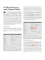
NCTUns provides more realistic wireless physical modules
that consider the used modulation scheme, the used
encoding/decoding schemes, the received power level, the
noise power level, the fading effects, and the derived BER
(Bit Error Rate) for 802.11(a), 802.11(b), 802.11(p), GPRS,
802.16(d) fixed WiMAX, 802.16(e) mobile WiMAX,
802.16(j) relay WiMAX, and DVB-RCST satellite networks.
These advanced physical-layer modules can generate more
realistic results but at the cost of more CPU time required to
finish a simulation. Depending on the tradeoff of simulation
speed vs. result accuracy, a user can choose whether to use
the basic simple physical-layer modules or the advanced
physical-layer modules.
It simulates multi-interface mobile nodes equipped with
multiple heterogeneous wireless interfaces. This type of
mobile nodes will become common and play an important
role in the real life, because they can choose the most costeffective network to connect to the Internet at any time and
at any location.
NCTUns supports omnidirectional and steerable antennas
with realistic antenna gain patterns. The antenna gain data
are stored in a table file and the content of the file can be
changed (even time-varying) easily if he (she) would like to
use his/her own antenna gain patterns.
Support for Various Networking Devices
NCTUns simulates common networking devices such as
Ethernet hubs, switches, routers, hosts, IEEE 802.11(b)
wireless access points and interfaces, IEEE 802.11(a)
wireless access points and interfaces, etc. For optical
networks, it simulates optical circuit switches and optical
burst switches, WDM optical fibers, and WDM protection
rings. For DiffServ QoS networks, it simulates DiffServ
boundary and interior routers for QoS provision. For GPRS
networks, it simulates GPRS phones, GPRS base stations,
SGSN, and GGSN devices. For 802.16(d) WiMAX
networks, it simulates the PMP-mode base stations (BS) and
Subscriber Stations (SS) and the mesh-mode base stations
and Subscriber Stations (SS). For 802.16(e) WiMAX
networks, it simulates the PMP-mode base stations (BS) and
Subscriber Stations (SS). For 802.16(j) transparent mode
and non-transparent mode WiMAX networks, it simulates
the base stations (BS), relay stations (RS), and mobile
stations (MS). For DVB-RCS network, it simulates the GEO
satellite, Network Control Center (NCC), Return Channel
Satellite Terminal (RCST), feeder, service provider, traffic
gateway. For wireless vehicular networks, it simulates ITS
cars each equipped with an 802.11(b) ad hoc-mode wireless
interface, ITS cars each equipped with an 802.11(b) infra-
Support for Various Network Protocols
NCTUns simulates various protocols such as IEEE 802.3
CSMA/CD MAC, IEEE 802.11 (a)(b)(e)(p) CSMA/CA
MAC, the learning bridge protocol used by switches, the
spanning tree protocol used by switches, IP, Mobile IP, RIP,
OSPF, UDP, TCP, HTTP, FTP, Telnet, etc. It simulates the
DiffServ QoS protocol suite, the optical light-path setup
protocol, the RTP/RTCP/SDP protocol suite. It simulates the
IEEE 802.16(d)(e)(j) WiMAX PMP protocol suites and the
802.16(d) mesh mode protocol suite. It simulates the DVBRCST protocol suite.
Highly-Integrated and Professional GUI Environment
NCTUns provides a highly-integrated and professional GUI
environment in which a user can easily conduct network
simulations. The NCTUns GUI program is capable of:
2
•
Drawing network topologies
•
Configuring the protocol modules used inside a node
•
Configuring the parameter values used inside a
protocol module
•
Specifying the initial locations and moving paths of
mobile nodes
•
Plotting network performance graphs
•
Playing back the animation of a logged packet transfer
trace
•
Pasting a map graph on the background of the network
topology
•
Constructing a road network for wireless vehicular
network simulations
•
More ...
simulation throughput when multiple machines are
available. Because the components of NCTUns use InterProcess Communication (IPC, that is, sockets) to communicate, they can also be run on the same machine. (This is
called the “single-machine” mode.). In fact, because most
people have only one computer to run their simulations, the
“single-machine” mode is the default mode after the
NCTUns package is installed. Switching between these two
modes is very easy and requires changing only one configuration option in a file.
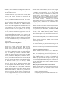
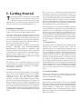
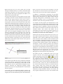
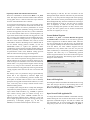
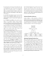
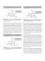
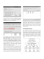
Components and Architecture of NCTUns
NCTUns adopts a distributed architecture. It is a system
comprising eight components.
Popular Operating System Support
NCTUns runs on Linux operating systems. The Linux distribution that NCTUns 6.0 currently supports is Red-Hat
Fedora 11, whose Linux kernel version currently is 2.6.28.9.
Other Linux distributions such as Debian can also be
supported with some minor operating system configuration
changes.
1 The first component is the GUI program by which a user
edits a network topology, configures the protocol modules
used inside a network node, specifies mobile nodes’ initial
location and moving paths, plots performance graphs,
plays back the animation of a packet transfer trace, etc.
2 The second component is the simulation engine program,
Open-System Architecture
which provides basic and useful simulation services (e.g.,
event scheduling, timer management, and packet manipulation, etc.) to protocol modules. We call a machine on
which a simulation engine program resides a “simulation
server.”
By using a set of well-defined module APIs that are provided
by the simulation engine, a protocol module developer can
easily implement his (her) own protocol and integrate it into
the simulation engine. Details about adding a new protocol
module to the simulation engine are presented in the “The
Protocol Developer Manual for the NCTUns 6.0 Network
Simulator and Emulator.”
3 The third component is the set of various protocol
modules, each of which implements a specific protocol or
function (e.g., packet scheduling or buffer management).
All protocol modules are C++ classes and are compiled and
linked with the simulation engine program.
Distributed Architecture for Remote and Concurrent Simulations
By using a distributed architecture, each component of
NCTUns can be run on a separate machine. (This is called
the “multi-machine” mode.) As such, the machine that runs
the GUI program can be different from the machine that runs
the simulation engine. This capability sometimes can have
an advantage; When simulating a very large case with
hundreds of mobile nodes, the GUI will consume many CPU
cycles to draw the movements of these mobile nodes during
the simulation. However, this will leave few CPU cycles for
the simulation engine to simulate the network protocols. To
overcome this performance problem, using the multimachine mode to run the GUI program and the simulation
engine on two different machines is a good solution.
4 The fourth component is the simulation job dispatcher
program that can simultaneously manage and use multiple
simulation servers to increase the aggregate simulation
throughput. It can be run on a separate machine or on a
simulation server.
5 The fifth component is the coordinator program. On every
simulation server, the “coordinator” program must be run
up. The coordinator should be alive as long as the
simulation server is alive. When a simulation server is
powered on and brought up, the coordinator must be run
up. It will register itself with the dispatcher to join in the
dispatcher’s simulation server farm. Later on, when the
status (idle or busy) of the simulation server changes, it
will notify the dispatcher of the new status. This enables
the dispatcher to choose an available simulation server
from its simulation server farm to service a job.
In addition, with the job dispatcher program, multiple
simulation engine machines can be managed by a single job
dispatcher. This architecture design can easily support
remote and concurrent simulations, which increases the total
3
When the coordinator receives a job from the dispatcher, it
forks a simulation engine process to simulate the specified
network and protocols. It may also fork several real-life
application program processes specified in the job. These
processes are used to generate traffic in the simulated
network.
Simulation
Server
Simulation
Server
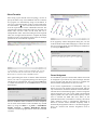
When the simulation engine process is alive, the coordinator communicates with the dispatcher and the GUI
program on behalf of the simulation engine process. For
example, the simulation engine process needs to periodically send its current simulation clock to the GUI program.
This is done by first sending the clock information to the
coordinator and then asking the coordinator to forward this
information to the GUI program. This enables the GUI
user to know the progress of the simulation.
Simulation
Server
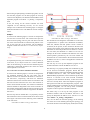
NCTU
Boston
GUI
Rome
GUI
Paris
GUI
Tokyo
Dispatcher
Simulation
Server
Simulation
Server
GUI
Background
Job Queue
Simulation Service Center
During a simulation, the GUI user can also on-line set or
get an object’s value (e.g., to query or set a switch’s current
switch table). Message exchanges that occur between the
simulation engine process and the GUI program are all
relayed via the coordinator.
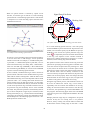
A Simulation Server ==
Kernel Modifications +
Simulation Engine +
Protocol Modules +
Coordinator
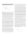
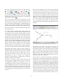
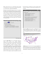
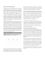
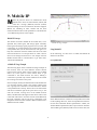
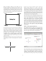
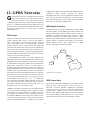
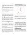
The distributed architecture of NCTUns.
6 The sixth component is the kernel patches that need to be
made to the kernel source code so that a simulation engine
process can run on a UNIX machine correctly. Currently
NCTUns 6.0 runs on Red-Hat’s Fedora 11, which uses the
Linux 2.6.28.9 kernel.
7 The seventh component is the various real-life user-level
application programs. Due to the novel kernel-reentering
simulation methodology, any real-life existing or to-bedeveloped application program can be directly run up on a
simulated network to generate realistic network traffic.
8 The eighth component is the various user-level daemons
that are run up for the whole simulation case. For example,
NCTUns provides RIP and OSPF routing daemons. By
running these daemons, the routing entries needed for a
simulated network can be constructed automatically. As
another example, NCTUns provides and automatically
runs up several emulation daemons when it is turned into
an emulator.
In addition to the above “multi-machine” mode, another
mode called the “single machine” mode is supported. In such
a mode, all of these components are installed and run on a
single machine. Although in this mode different simulation
jobs cannot be run concurrently on different machines, since
most users have only one machine to run their simulations,
this mode may be more appropriate for them. In fact, it is the
default mode after the NCTUns package is installed.
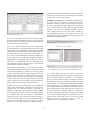
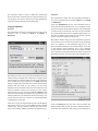
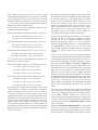
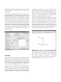
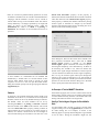
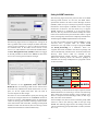
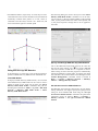
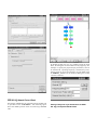
Some Screenshots of NCTUns
To give readers a quick idea about what the GUI
environment looks like, some screenshots of NCTUns are
shown below.
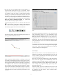
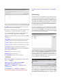
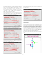
Starting Screen
Every time when a user launches the GUI program, the
following starting screen will pop up.
Due to this distributed design, a remote user can submit his
(her) simulation job to a job dispatcher, and the dispatcher
will then forward the job to an available simulation server for
execution. The server will process (simulate) the job and
later return the results back to the remote GUI program for
further analyses. This scheme can easily support the server
farm model in which multiple simulation jobs are performed
concurrently on different simulation servers. The following
figure shows the distributed architecture of the NCTUns.
4
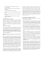
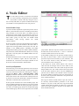
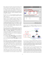
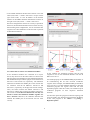
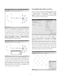
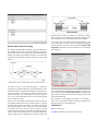
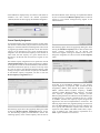
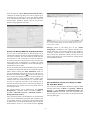
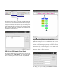
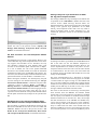
Topology Editor
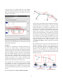
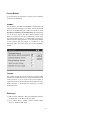
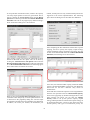
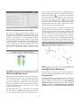
Performance Monitor
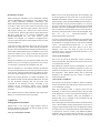
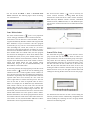
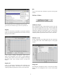
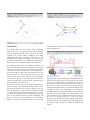
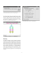
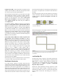
The topology editor provides a convenient and intuitive way
to graphically construct a network topology. A constructed
network can be a fixed wired network or a mobile wireless
network. For ITS applications, a road network can also be
constructed. Due to the user-friendly design, all GUI operations can be performed easily and intuitively.
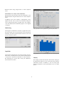
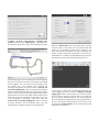
The performance monitor can easily and graphically
generate and display plots of some monitored performance
metrics over time. Examples include a link’s utilization or a
TCP connection’s achieved throughput. Because the format
of its input data log file uses the general two-column (x, y)
format and the data is in plain text, the performance monitor
can be used as an independent plotting tool.
The topology editor of NCTUns
The performance monitor of NCTUns
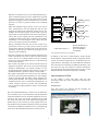
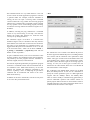
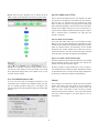
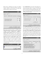
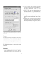
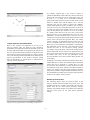
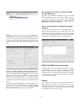
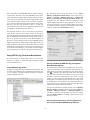
Attribute Dialog Box
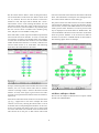
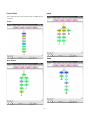
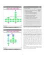
Node Editor
A network device (node) may have many attributes. Setting
and modifying the attributes of a network node can be easily
done. Just double-clicking the icon of a network node. An
attribute dialog box pertaining to this node will pop up. A
user can then set the device’s attributes in the dialog box.
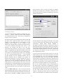
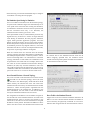
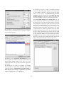
The node editor provides a convenient environment in which
a user can flexibly configure the protocol modules used
inside a network node. By using this tool, a user can easily
add, delete, or replace a module with his (her) own module.
This capability enables a user to easily test the performance
of a new protocol.
Using the node editor, a user can also conveniently set the
parameter values used by a specific protocol module. Each
box in the node editor represents a protocol module. A user
can double-click a protocol module box to pop up its
parameter dialog box.
Regarding how to add a new protocol module to the node
editor (i.e., to let it know that a user has added a new protocol
module to the simulation engine), readers should refer to the
“The Protocol Developer Manual for the NCTUns 6.0
Network Simulator and Emulator.”
A popped-up dialog box of NCTUns
5
package. To let readers quickly get a feel of the operations of
this tool, a short tour about running a simple simulation case
will be presented in the next chapter.
Reference
[1] S.Y. Wang and H.T. Kung, “A Simple Methodology for
Constructing Extensible and High-Fidelity TCP/IP
Network Simulator,” IEEE INFOCOM’99, March 2125, 1999, New York, USA.
[2] S.Y. Wang and H.T. Kung, “A New Methodology for
Easily Constructing Extensible and High-Fidelity
TCP/IP Network Simulators,” Computer Networks, Vol.
40, Issue 2, October 2002, pp. 257-278.
[3] S.Y. Wang, “NCTUns 1.0,” in the column “Software
Tools for Networking,” IEEE Networks, Vol. 17, No. 4,
July 2003.
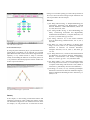
The node editor of NCTUns
[4] S.Y. Wang, C.L. Chou, C.H. Huang, C.C. Hwang, Z.M.
Yang, C.C. Chiou, and C.C. Lin, “The Design and Implementation of NCTUns 1.0 Network Simulator,”
Computer Networks, Vol. 42, Issue 2, June 2003, pp.
175-197.
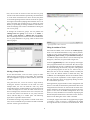
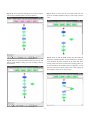
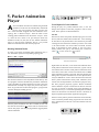
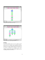
Packet Animation Player
By using the packet animation player, a packet transfer trace
logged during a simulation can be replayed at a specified
speed. Both wired and wireless networks are supported. This
capability is very useful because it helps a researcher
visually see and debug the behavior of a network protocol. It
is very useful for educational purposes because students can
see how a protocol behaves.
[5] S.Y. Wang and Y.B. Lin, “NCTUns Network Simulation
and Emulation for Wireless Resource Management,”
Wireless Communication and Mobile Computing,
Wiley, Vol. Issue 8, pp. 899 ~ 916, December 2005.
[6] S.Y. Wang and K.C. Liao, “Innovative Network Emulations using the NCTUns Tool,” as a book chapter of the
“Computer Networking and Networks” book, (ISBN 159454-830-7, published by Nova Science Publishers)
[7] S.Y. Wang, C.L. Chou, C.C. Lin, “The Design and Implementation of the NCTUns Network Simulation Engine,”
Elsevier Simulation Modelling Practice and Theory, 15
(2007) 57 -81.
The packet animation player of NCTUns
Summary
In this chapter, we have briefly presented the features and
capabilities of NCTUns. After reading this chapter, readers
now should have a high-level view about NCTUns 6.0. In the
next chapter, we will present how to install the NCTUns
6
2. Getting Started
Due to the use of a novel kernel-reentering simulation
methodology, NCTUns has two advantages as follows: (1)
Any real-life application program can be run on a simulated
network to generate traffic and (2) Their performance can be
evaluated under different simulated network conditions.
Thus the real-life application programs pre-installed in this
directory represent only a very small subset of real-life application programs that can be used with NCTUns.
his chapter presents a simple tour to help readers
quickly learn how to use NCTUns. First, we give
instructions on how to install NCTUns on a single
machine. Next, we present step-by-step instructions to illustrate how to quickly run up a simple simulation case.
T
During simulation, if a user wants the simulation engine to
run up an application program that is not pre-installed in this
subdirectory (e.g., the P2P BitTorrent program), the user
must first copy that program into this subdirectory (i.e.,
/usr/local/nctuns/tools) so that the simulation engine can find
it during simulation. Detailed information on how to specify
which application programs should be run on which nodes in
the GUI program is presented in the “Topology Editor”
chapter.
Installation and Configuration
In the following, we assume that when installing the
package, the user uses the package’s default settings.
A user first downloads the package from the web site at
http://NSL.csie.nctu.edu.tw/nctuns.html. Starting from the
2.0 version, the operating systems that NCTUns supports is
only Linux and FreeBSD is no longer supported. Right now,
the Linux distribution supported is Red Hat’s Fedora 11,
which uses Linux kernel version 2.6.28.9.
3. /usr/local/nctuns/etc
This directory stores the configuration files needed by the
dispatcher and coordinator programs. Their names are
“dispatcher.cfg,” and “coordinator.cfg,” respectively. Some
other configuration files used by NCTUns are also stored
here. For example, the “app.xml,” which is read by the GUI
program to explain the usages of pre-installed application
programs, is also stored here. An “mdf” subdirectory (which
stands for “module definition file”) is created here. Inside
this directory, the parameter definitions and dialog box
layout design of supported protocol modules are stored in
separate subdirectories. The GUI program will read the files
inside the mdf directory to know the definition of supported
protocol modules. The “ps.cfg” file describes the default
internal protocol stack used by each supported network
node.
After reading the installation explanations and instructions
(INSTALL, README, FAQ, KNOWN.PROBLEM,
RELEASE.NOTE) and running the installation script
(install.sh), a directory named “nctuns” will be created in the
/usr/local/ directory, which in turn has several subdirectories.
The name of these subdirectories are “bin,” “etc,” “tools,”
“BMP”, and “lib,” respectively. In the following, we explain
each of these subdirectories briefly.
1. /usr/local/nctuns/bin
This directory stores executable programs of the GUI
program, dispatcher, coordinator, and the simulation engine.
Their names are “nctunsclient,” “dispatcher,” “coordinator,”
and “nctunsse,” respectively.
2. /usr/local/nctuns/tools
4. /usr/local/nctuns/BMP
This directory stores executable programs of various applications and tools pre-installed by NCTUns. For example,
currently “stcp,” “rtcp,” “ttcp,” “tcpdump,” “ripd,” “ospfd,”
“nctunstcsh,” “script,” “stg,” “rtg,” “tsetenv,” “ifconfig,”
and “ping” are supported. Some daemon programs used by
NCTUns are also stored in this directory. For example, the
daemon programs used for emulation and Mobile IP are
stored here. The agent programs that are used for tactical and
active mobile ad hoc network simulations (e.g., “Magent1”)
are also stored here. These tactical agent programs can be run
on mobile nodes to control the moving behavior of mobile
nodes.
This directory stores the icon bmp files used by the GUI
program. These icon files are used for displaying various
devices’ icons and control buttons.
5. /usr/local/nctuns/lib
This directory stores the libraries used by the simulation
engine. For example, the more advanced signal propagation
model library used by IEEE 802.11(b) advanced wireless
physical module is installed here. NCTUns supports
RTP/RTCP/SDP protocols and implements some of their
functions as a library that can be called by RTP/RTCP/SDP
application programs.
7
Before a user can run up the dispatcher, the coordinator, and
the GUI programs, he (she) must first set up the NCTUNSHOME environment variable. To do so, a user can type in
and execute the “setenv NCTUNSHOME /usr/local/nctuns/”
shell command in his (her) terminal window (i.e., xterm) if
the csh or tcsh shell is used. For the bash shell, the command
should be “export NCTUNSHOME=/usr/local/nctuns.” Two
other environment variables must be set as well. The first is
NCTUNS _TOOLS and the second is NCTUNS_BIN. They
must
be
set
to
/usr/local/nctuns/tools
and
/usr/local/nctuns/bin, respectively.
Installation Procedure
Before starting the installation, a user should first carefully
read the “README” and “INSTALL” files. Both of these
files contain important installation information. The
RELEASE.NOTE file contains notes relevant to each release
of NCTUns. These notes point out the new functions, bug
fixes, performance and GUI improvements, data structure
and program changes, etc. between the current and the
previous releases. The FAQ file answers technical questions
that may result due to an incorrect installation. The
KNOWN.PROBLEM file lists some known system
problems. For example, if a computer is equipped with a
very new video card, the new video card driver may not work
well with Fedora 11.
For a user’s convenience, the installation script will place the
nctuns.csh and nctuns.bash file in /usr/local/nctuns/etc when
the installation is completed. The user can use the command
“source /usr/local/nctuns/etc/nctuns.csh” to set these
environment variables if his (her) shell is csh or tcsh.
Similarly, if the user uses bash, he (she) can use the
command “source /usr/local/nctuns/etc/nctuns.bash” to set
these environment variables.
A user then runs the “install.sh” shell script. This script will
install the pre-compiled Linux kernel image patched for
NCTUns. It will also build all executable programs and copy
them to their default subdirectories. In addition, it will create
4,096 (this number can be easily increased) tunnel special
files (tunnel interfaces) in /dev. These steps may take some
time.
2. Start up the dispatcher
Now a user can run up the dispatcher, which is located in
/usr/local/nctuns/bin. Note that the user must be the root user
to run dispatcher correctly.
During the installation, the user should carefully watch out
whether some error messages are generated. If any serious
error message is generated, the installation may fail.
The default port number used by the dispatcher to receive
messages sent from the coordinator program(s) is 9,810. It is
9,800 for the dispatcher to receive messages sent from the
GUI program(s). These default settings can be found and
changed in the dispatcher.cfg file, which is located in
/usr/local/nctuns/etc/.
After the installation is successfully finished, the machine
must be rebooted and then the user must choose the NCTUns
kernel to boot. After the machine boots up with the NCTUns
kernel, the whole installation can be considered successful.
Before start running NCTUns to conduct simulations, the
user should carefully read the FINALCHECK file. This file
lists the important operations that the user must have
performed to run NCTUns correctly. According to our
technical service experiences, almost every reported
problem is caused by not performing all of these required
operations.
3. Start up the coordinator
Now the user can run up the coordinator, which is located in
/usr/local/nctuns/bin. Note that the user must be the root user
to run coordinator correctly.
Since the coordinator needs to register itself with the
dispatcher, we must let the coordinator know the port used
by the dispatcher to receive the registration messages. (It is
9,810 in the above example.) This port information is
specified and can be changed in the coordinator.cfg file
located in /usr/local/nctuns/etc/.
More detailed and up-to-date installation and usage information can be found in the NCTUns package.
A Quick Tour
Setting up the environment
The second important information that the coordinator must
know is the IP address used by the dispatcher. If the user is
using the single-machine mode, since the dispatcher and the
coordinator are run on the same machine, the IP address can
be specified as 127.0.0.1, which is the default IP address
assigned to the lo loopback network interface. In case the
127.0.0.1 IP address cannot work due to some unexpected
Suppose that a user uses the single-machine mode of
NCTUns, before he (she) starts the GUI program, he (she)
must perform three operations.
1. Set up environment variables
8
It is important to note that only in the “Draw Topology”
mode can a user draw a new network topology or change
an existing simulation case’s topology. When a user
switches the mode to the next mode “Edit Property,” the
simulation case’s network topology can no longer be
changed. Instead, only devices’ properties (attributes) can
be changed at this time.
reasons, the user can replace it with the machine’s own IP
address (e.g., 140.113.17.5). This setting should always
work.
If a user is using the multi-machine mode and the dispatcher
is running on a remote machine, the IP address specified
should be the IP address of that remote machine.
4. Start up the nctunsclient
The GUI program enforces this rule because when the
mode is switched to the “Edit Property” mode, for the
user’s convenience, the GUI program will automatically
generate many settings (e.g., a layer-3 interface’s IP and
MAC addresses). Since the correctness of these settings
depends on the current network topology, if the network
topology gets changed, these settings may become
incorrect.
After all of the above steps are performed, a user can now
launch NCTUns’s GUI program (called nctunsclient). This
program is also located in /usr/local/nctuns/bin. To run the
GUI program successfully, the user need not be the root user.
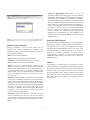
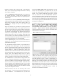
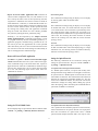
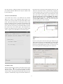
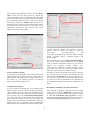
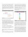
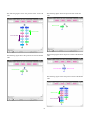
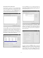
Draw a Network Topology
After the starting screen of NCTUns disappears, a user will
be presented a working window shown below.
If after editing some devices’ properties, the user would
like to change the network topology, he (she) will need to
explicitly switch the mode back to the “Draw Topology”
mode. However, when the mode is switched from the
“Draw Topology” mode back to the “Edit Property” mode
again, many settings that were automatically generated by
the GUI program will be re-generated automatically by the
GUI program to ensure their correctness.
For example, the IP and MAC addresses automatically
assigned to a layer-3 network interface may have been
changed. The user thus better re-checks the settings for
application programs (traffic generator) that he (she)
specified when he (she) was in the “Edit Property” mode.
This is because these application programs now may use
wrong IP addresses to communicate with their intended
partners.
The working area of the topology editor
2. Move the mouse cursor to the tool bar, which is shown
below.
To edit a new network topology, a user can perform the
following steps.
1. Choose Menu->File->Operating Mode and make sure
that the “Draw Topology” mode is checked. Actually, this
is the default mode which NCTUns will be in when it is
launched.
3. Left-click the router icon (
) on the toolbar.
4. Left-click somewhere in the blank working area to add a
router to the current network topology (which is empty
now).
5. Left-click the host icon (
9
) on the toolbar.
like text format. This allows a user to easily view and
check the stored attribute values.
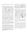
Like in step 4, add three hosts to the current network
topology. The resulting topology is shown below.
6. Now we want to add links between the hosts and the
router. Left-click the link icon (
) on the toolbar to
select it.
It is not mandatory to save the network topology into a file
in this mode. A user can save it in the “Edit Property” mode.
Depending on in which mode a network topology file was
saved, when the file is opened again, its current mode will be
automatically set to the mode when it was saved.
7. Left -click a host and hold the mouse button. Drag this link
to the router and then release the mouse left button on top
of the router. Now a link between the selected host and the
router has been created.
8. Add the other two links in the same way. Now the simple
network topology has been created.
Editing Nodes’ Properties
A network node (device) may have many parameters to set.
For example, we may want to set the maximum queue length
of a FIFO queue used inside a network interface. For another
example, we may want to specify that some application
programs (traffic generators) should be run up on some hosts
or routers to generate network traffic.
Before a user can start editing the properties of network
nodes, he (she) should switch the mode from the “Draw
Topology” to the “Edit Property” mode. In this mode,
topology changes can no longer be made. That is, a user
cannot add or delete network nodes or links at this time. If
the user has not given a name to this simulation case, the GUI
program will pop up a dialog box at this time asking the user
to specify one.
To save the user’s configuration time, the GUI program
automatically finds subnets in a fixed network, and generates
and assigns IP and MAC addresses to all layer-3 network
interfaces. In addition, the GUI program automatically
generates and assigns MAC addresses to layer-2 network
interfaces. Note that layer-3 interfaces are used by layer-3
9. Remember to save this network topology by choosing
Menu -> File -> Save As. For this simple case, we will
save the topology file as “test.tpl.” When the GUI
program creates test.tpl, it also creates test.xtpl. This file
stores the attribute values stored in test.tpl in an XTML-
10
limitation can be easily raised to a larger number such as
8,192 by creating more tunnel interfaces on the simulation
machine. This change can be easily done by modifying the
installation script.
devices such as hosts, routers, and mobile nodes, and layer2 interfaces are used by layer-2 devices such as switches and
wireless LAN access points.
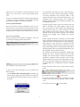
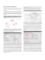
The generated IP addresses use the 1.0.subnetID.hostNumOnThisSubnet format, where subnetID and hostNumOnThisSubnet are automatically assigned. The IP and
MAC addresses generated and assigned to an interface can
be known easily. When a user moves the mouse cursor onto
a blue box, which represents a network interface, the IP
address assigned to it along with the port ID assigned to it
will be shown. The following figure shows an example.
The used subnet number starts from 1 and automatically
grows upward. The used host number on a subnet also starts
from 1 and automatically grows upward. If there are WLAN
ad-hoc mode mobile nodes in the network, the subnet ID 1 is
reserved and used for the ad-hoc subnet formed by these adhoc mode mobile nodes. In such a case, the subnet number
used for fixed subnets will start from 2. On the other hand, if
there is no ad-hoc mode mobile node in the network, the
subnet number used for fixed subnets will start from 1.
The GUI program can automatically generate and assign IP
addresses to ad-hoc mode mobile nodes (
or
), hosts,
and routers on the fixed network. For infrastructure mode
mobile nodes (
or
), however, the GUI program needs
helps from the “form subnet” (
) tool to automatically
generate and assign IP addresses to them. The full name and
location of this tool are shown in the following figure. More
information on the usage of this tool will be presented in a
later chapter.
Due to this address format, NCTUns allows a simulation
case to have up to 254 subnets (subnet ID 0 and 255 are
excluded because they are used for broadcast purposes),
each of which can have up to 254 nodes (hostNum 0 and 255
are excluded because they are used for broadcast purposes).
That is, in total a maximum number of 254 * 254 = 64,516
layer-3 interfaces can be supported in a simulation case.
Although in theory NCTUns can support this large number
of layer-3 interfaces in a simulation case, in practice this is
rarely done. This is because each layer-3 interface needs to
be simulated by a tunnel network interface but currently the
installation script creates only 4,096 tunnel interfaces on a
UNIX machine by default. So, precisely speaking, currently
NCTUns can support a simulation case using up to 4,096
layer-3 interfaces. This also means that currently the
maximum number of mobile nodes in a mobile ad-hoc
network simulation case cannot exceed 4,096. (This is
because each mobile node uses a layer-3 interface.) This
The reason is that an infrastructure mode mobile node needs
to use an access point to connect itself to the fixed network.
To successfully send and receive packets to and from the
fixed network, the infrastructure mode mobile node needs to
use an IP address whose subnet ID is the ID of the subnet that
the access point belongs to. However, during the automatic
IP address generation process, the GUI program does not
have the intelligence to know which subnet the user would
like an infrastructure mode mobile node to belong to (e.g.,
11
when a user moves the mouse cursor and place it over the
blue interface box on the screen for a while. This can conveniently let the user see the results of these assignments.
suppose that there are two access points each of which
belongs to a different subnet). As a result, without the subnet
relationship information, the GUI program cannot intelligently generate and assign an appropriate IP address to an
infrastructure mode mobile node.
In addition to automatically generating IP and MAC
addresses, the GUI program also automatically and silently
performs many tasks for the user. Many of these tasks are
performed underground to automatically correct a user’s
configuration mistakes. This is to avoid generating wrong
simulation results and causing simulation crashes.
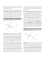
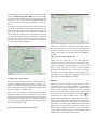
To help the GUI program solve this problem, the user needs
to manually select the involved infrastructure mode mobile
nodes and the desired wireless access point to form a
wireless subnet. With this subnet grouping information, the
GUI program now knows the access point with which these
infrastructure mode mobile nodes would like to associate. As
a result, it knows the subnet ID that should be assigned to this
wireless subnet and it can assign a unique and correct IP
address to each of these infrastructure mode mobile nodes
automatically. With this design, the user need not configure
the gateway IP address for these infrastructure mode mobile
nodes. The GUI program intelligently knows this information by tracking the access point back to the router that
has a network interface connecting to this access point. The
IP address of this network interface is the gateway IP address
for these infrastructure mode mobile nodes. The following
figure shows that the “form subnet” tool is used to select two
infrastructure mode mobile nodes and one access point to
form a wireless subnet.
For example, the GUI program will automatically set the
promiscuous mode of the 802.3 MAC modules that are used
inside a switch to ON, no matter how the user set them. (The
promiscuous mode is defaulted to OFF because the 802.3
MAC modules used inside hosts and routers need to filter out
unwanted frames.) This ensures that frames can be
forwarded by the switch without any problem. Otherwise, if
the promiscuous mode is not turned ON, frames will be
discarded by the switch’s 802.3 MAC modules.
Another task that the GUI program does for the user is to
ensure that all interfaces that connect to a hub uses the hub’s
bandwidth as their interface bandwidth and the operating
mode of the 802.3 MAC modules in these interfaces all be
set to “half-duplex.” In the GUI program, a user can independently set different bandwidths for different interfaces and
set an 802.3 MAC module’s mode to either “full-duplex” or
“half-duplex” without considering whether these interfaces
are connected to a hub. These wrong configurations surely
will generate wrong simulation results and may even cause a
simulation to crash. This kind of wrong configuration bug is
difficult to detect for a careless user. As a result, the GUI
program does several underground tasks to save the user’s
debugging time and increase his (her) productivity.
Yet another task that is automatically done by the GUI
program is that the GUI program will force the switch
module used inside an access point (
or
) to use the
“Run_Learning_Bridge” mode, despite the fact that the user
may configure it to use the “Build in Advance.” These two
modes affect how the switch forwarding table used inside the
switch module is built. The first method is a dynamic method
while the second is a static one. The second method works
very well for fixed networks. However, in mobile networks
where mobile nodes move around and change their
associated access points constantly, the static method will no
longer work correctly. To prevent the user from suffering
unexpected (wrong) simulation behavior and results, the
GUI program automatically forces the switch module used
A user must be aware that if he (she) switches the mode back
to the “Draw Topology” mode, when he (she) again switches
the mode back to the “Edit Property” mode, nodes’ IP and
MAC addresses will be re-generated and assigned to layer-3
interfaces. Therefore the application programs (traffic
generator) now may use wrong IP addresses to communicate
with their partners.
In this mode, since the IP and MAC addresses and the port
ID of an interface have been automatically generated and
assigned, the GUI will automatically show these information
12
inside all access points to use the “Run_Learning_Bridge”
method to dynamically build and update their forwarding
tables.
Therefore, in the future when you see that the GUI program
does not honor your settings for some devices or protocol
modules, do not be surprised. You know that the GUI
program is doing this for your good.
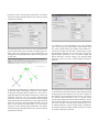
Editing network nodes’ properties can be done in two steps.
In the first step, a user can use the mouse to double-click a
node’s icon. A dialog box will appear in which a user can set
parameter values or option values. The following figure
shows an example dialog box after the user double-clicks the
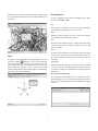
router icon.
The popped-up node editor for the router node
cars, multi-interface nodes, 802.11(p) OBU and RSU, etc.
Actually, as long as a node has a layer-3 interface (which
should have an IP address assigned to it), any application
program can run on it. In such devices’ dialog boxes, there is
an “Application” tab in which a user can specify the
commands for launching the desired application programs.
For example, suppose that a user wants to sets up a greedy
TCP connection between two nodes. He (she) can specify the
command “rtcp -p 8000” on the receiving node’s Application
tab and specify the command “stcp -p 8000 1.0.1.2” on the
sending node’s Application tab. In this case, stcp and rtcp are
the pre-installed real-life application programs that will
greedily send and receive TCP data, respectively. Also, we
assume that the receiving node has an assigned IP address of
1.0.1.2 and the rtcp program binds its receiving socket to port
8000.
The router’s dialog box
In the second step, a user can use the node editor to specify
the protocol module parameters used inside a network node.
To enter the node editor, a user first double-clicks the node’s
icon to pop up its dialog box. Then the user double-clicks the
“node editor” button in the dialog box. The following figure
shows the popped node editor and the protocol modules used
inside the router.
From the above example, one sees that the specified
commands are exactly the same as what a user would type
into a UNIX terminal to launch (run up) these application
programs.
One important task in the “Edit Property” mode is to specify
which application programs (traffic generators) should run
on which nodes during simulation to generate network
traffic. Application programs can run on hosts, routers,
mobile nodes (including both the ad-hoc and infra-structure
modes), GPRS phones, IEEE 802.16(d) WiMAX BS and SS,
IEEE 802.16(e) mobile WiMAX BS and MS, IEEE
802.16(j) relay WiMAX BS, RS, and MS, DVB-RCST, ITS
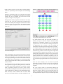
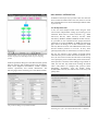
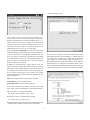
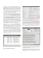
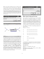
The “App. Usage” button in the following dialog box
provides command usage information for each pre-installed
application program. When a GUI user double-clicks this
button, a program usage information window will pop up
showing the detailed usage for each pre-installed application
13
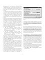
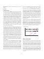
the program’s usage information into that file. The format of
this file is easy to understand. The following figure shows
the content of the /usr/local/nctuns/etc/app.xml file.
In the application tab a user can specify which application
programs should be run up on this node.
The content of the program usage information file (app.xml).
Running the simulation
program. The following figure shows the content of this
window. For the first use, the user needs to click the
“Refresh” button to get the latest program usage information
from the (may be local or remote) dispatcher.
When a user finishes editing the properties of network nodes
and specifying application programs to be executed during a
simulation, he (she) can start to run the simulation. To do so,
the user must switch the mode explicitly from “Edit
Property” to “Run Simulation.” Entering this mode indicates
that no more changes can (should) be made to the simulation
case, which is reasonable. The simulation is about to be
started. At this moment, of course, no settings should be
changed.
When the mode is switched to the “Run Simulation” mode,
the GUI will export many simulation files that collectively
describe the simulation case. These simulation files will be
transferred to the (either remote or local) simulation server
for it to execute the simulation. These files are stored in the
“mainFileName.sim” directory, where mainFileName is the
name of this simulation case.
For example, suppose that the topology file is named
“test.tpl,” these exported simulation files will be stored in a
directory named “test.sim.” Among these exported files, the
test.tcl file stores the configuration of each node’s protocol
stack and the network topology information. This file is very
important and should always go with the test.tpl and test.xtpl
files. Therefore, if a user wants to move (or copy) a
simulation case from one place to another place in a file
system, he (she) must move (or copy) the .tpl and .xtpl files
and their associated .sim directory at the same time.
Otherwise, the moved (or copied) simulation case cannot be
successfully reloaded. For this particular example, he (she)
must move test.tpl, test.xtpl, and test.sim/ at the same time.
The content of the program usage information window.
If a GUI user wants to install a new application program, he
(she) needs to copy that program into the
/usr/local/nctuns/tools directory so that the simulation
engine can successfully find and execute it. If the GUI user
also wants the usage information of this new program to be
displayed in the above program usage window, he (she)
needs to edit the /usr/local/nctuns/etc/app.xml file and put
14
In addition to the “.sim” directory, a directory named
“mainFileName.results” is also created. This directory will
store the generated simulation results when they are transferred back to the GUI program after the simulation is
finished.
It is important to note that before a user runs a simulation
case, he (she) can still switch the mode back to the “Edit
Topology” or even the “Draw Topology” mode to change
any setting of the simulation case. However, when the mode
is switched back to the “Run Simulation” mode, all
simulation files will be re-exported to reflect the most recent
settings.
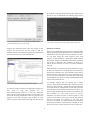
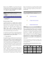
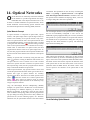
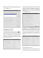
The popped-up dialog box for setting dispatcher-related information.
Before a user runs a simulation, he (she) must make sure that
the dispatcher and coordinator are already running. Suppose
that the user uses the single-machine mode of NCTUns, he
(she) needs to run up the dispatcher and coordinator
programs first. The following procedure assumes that the
user uses the single-machine mode. If the user uses a
simulation service center (running in the multi-machine
mode) that is already set up by some person or institute, he
(she) can skip the following two steps.
1.
Run the “dispatcher” program located in
/usr/local/nctuns/bin. The default values of the parameters
needed
by
this
program
is
stored
in
/usr/local/nctuns/etc/dispatcher.cfg.
2.
Run the “coordinator” program located in
/usr/local/nctuns/bin. The default values of the parameters
needed
by
this
program
is
stored
in
/usr/local/nctuns/etc/coordinator.cfg.
guarantee this property, normally a simulation service center
will use NFS (network file system) and YP password facilities. This will make sure that all machines in this service
center share the same user account database and share the
same file system.
The user name specified in this dialog box cannot be “root.”
That is, the GUI user should not use the root account to log
onto a simulation server, no matter whether it is a local or
remote machine. This enforcement is for security concerns.
Also, if the GUI user logs on a simulation server as the “root”
user, he (she) will not be able to use the command console
function correctly. For these reasons, the “root” account is
blocked here by the GUI program.
During simulation (i.e., when the simulation is not finished
yet), the result files generated by the simulation engine are
stored in a working directory inside the home directory of the
provided user account. Hence, this user account information
must be correct and valid. Otherwise, the GUI program will
crash due to access permission errors. Specifying the email
address is not mandatory. However, if this information is
provided, a remote dispatcher can send back a notification
email to the user when the user’s background job is finished
in its simulation service center. Currently, this notification
function is not implemented.
Now the user needs to let the GUI program know the IP
address and port number used by the dispatcher. The user
should configure these settings by invoking the Menu ->
G_Setting -> Dispatcher command. The following figure
shows the popped-up dialog box.
The default port number is 9,800. If the user is using the
single-machine mode, the IP address can be specified as
127.0.0.1, which is the default IP address that the UNIX
system automatically assigns to the loopback interface. The
user name and password must be valid. For the singlemachine mode, it is the user’s account on this local machine.
For the multi-machine mode, it is the user’s account on the
chosen remote simulation machine.
Since we have specified a complete simulation case and we
are certain that the dispatcher and coordinator programs are
running, we can now proceed to run the simulation.
3. Choose Menu -> File -> Operating Mode and select
“Run Simulation”.
Note that in the multi-machine mode, because simulations
are actually performed on a simulation server machine, the
user must also have the same account on any simulation
server machine that is managed by the dispatcher. To
15
To save the network bandwidth and time required for transferring these huge files across a network, these result files are
tarred (using the tar command) and gzipped (using the gzip
command) into a tar ball before being sent to the GUI
program. This usually can reduce the bandwidth usage by a
factor of 10 or above. After receiving the tar ball, the GUI
program needs to untar and ungzip the tar ball before using
these files. As a result, a user may experience some delay up
to a few minutes (depending on the machine’s speed)
without any progress update on the screen. At this moment,
the user needs to be patient.
These files include a packet animation trace file and all
performance log files that the user specified to generate.
Generating these performance log files can be specified by
checking some output options in some protocol modules
(e.g., 802.3 or 802.11(b) protocol modules) in the node
editor. In addition, application programs can generate their
own data log files. For example, the pre-installed “rtg”
program can be specified to output a performance log file
showing the end-to-end delays experienced by all received
packets.
4. Choose Menu -> Simulation -> Run. Executing this
command will submit the current simulation job to one
available simulation server (or the only local simulation
server) managed by the dispatcher.
The packet animation trace file can be replayed later by the
packet animation player. The performance curve of these log
files can be plotted by the performance monitor. Details
about the animation player and the performance monitor will
be explained in later chapters.
For this simple case, the packet animation trace file is named
“test.ptr,” which uses the main file name of the topology file
-- “test.tpl.” The .ptr file is a logged packet transfer trace file.
Its animation can be played by the animation player at a
specified speed. To save disk space and transfer time, the .ptr
is a binary file, which means that its content cannot be
directly viewed using a normal text editor such as vi or
emacs. To allow a user to convert it into a text file for
inspection, a “printPtr” utility program is provided in
/usr/local/nctuns/bin. In addition, the user can also execute
the GUI’s Menu -> G_Tools -> View Packet Trace
command to view a simulation case’s .ptr file.
5. When the simulation server is executing, the user will see
the time knot at the bottom of the screen move. The time
knot reflects the current simulation time (progress) of the
simulation case. Currently, the maximum time that can
be simulated for a simulation case is set to 4,200
seconds.
When the GUI program has untarred and ungzipped the .ptr
file, it will automatically switch to the “Play Back” mode. In
this mode, the control buttons of the time bar located at the
bottom of the screen can be used to play, stop, pause,
continue, jump forward, jump backward, or “intelligently”
jump forward the animation.
Playing Back the Packet Animation Trace
After the simulation is finished, the simulation server will
send back the simulation result files to the GUI program.
After receiving these files, the GUI program will store these
files in the “.results” directory. It will then automatically
switch to the “Play Back” mode.
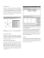
The user can also use the mouse to directly move the time
knot to any desired time to see the packet transfers occurring
at that moment. To precisely move the time knot to a specific
16
time, the user can even double-click the time-display (i.e.,
the LCD clock display) area to pop up a window. In this
window, the user can directly enter the desired time in ticks.
For example, if the user wants to see the packet transfers
occurring at 1.2345678 seconds, then he (she) can enter
12345678 into this window. The default mapping between 1
tick and its corresponding time duration in simulation time is
1 tick -> 100 nanoseconds. This mapping can be changed by
Menu->G_Setting->Simulation->Speed for high-speed
networks such as 1 Gbps optical networks.
To start the playback, the user can left-click the start icon
(
) of the time bar located at the bottom. The animation
player will then start playing the recorded packet animation.
The following figure shows these control buttons.
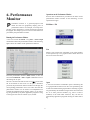
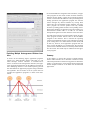
The performance plotter is plotting a performance curve over
time.
Note that the performance monitor can also be used to plot
static performance graphs (i.e., the performance curves
during a fixed time interval) and this can be easily done.
When the packet animation player is not playing (i.e.,
stopped), the user can directly move the time knot to any
desired time. This will cause the performance monitor to plot
static performance curves over a time interval that starts at
the specified time.
The following figure shows the animation player when it is
playing a packet animation trace file.
At this stage, the whole process of using NCTUns to perform
a simulation case is over. The user may quit the GUI program
at this time while leaving the dispatcher and coordinator
program running in the background.
Post Analyses
When the user wants to review the simulation results of a
simulation case that has been finished before, he (she) can
run up the GUI program again and then open the case’s
network topology file (.tpl).
The user can switch the mode directly to the “Play Back”
mode. The GUI program will automatically reload the
simulation results (including the packet animation trace file
and some performance log files). Because the animation file
size is usually very large, the loading process may take a
while for a large case.
While the packet animation player is running, the user can
also launch the performance monitor. In this way, the performance monitor will dynamically plot performance curves of
some logged performance metrics as the time is progressing.
For example, a TCP connection’s achieved throughput or a
link’s utilization can be plotted. The time used by the performance monitor and the packet animation player are synchronized with each other. The following figure shows the
performance monitor when it is plotting a performance curve
over time.
After the loading process is finished, the user can use the
control buttons located at the bottom of the screen to view
the animation, just like what he (she) would do when a
simulation job is done.
17
•
Submit as Background Job: Submit a job to the
dispatcher without first running up it in the GUI and then
immediately disconnecting it. Its net effect is the same as
first running up a simulation job and then immediately
disconnecting the GUI program from it. A job submitted in
this way is called a “background job.” It does not need the
GUI’s support (or occupy the GUI) while its simulation is
ongoing. A background job may wait in the dispatcher’s
job queue if currently there is no available simulation
server to service this job. Whenever a simulation server
becomes available, on behalf of the GUI program that
submitted this background job, the dispatcher will
automatically start the background job’s execution on that
simulation server.
Background Job Management
As explained before, a background job is a job submitted by
executing the “Submit” command. After being submitted, a
background job may (1) wait in the dispatcher’s job queue
waiting for an available simulation server to service it, (2) be
currently executed by a simulation server, or (3) may have
finished its simulation. Depending on which state a
background job is currently in, a user can use appropriate
commands to either cancel it, reconnect to it, or retrieve its
simulation results.
Simulation Control Commands
During a simulation, a user can have control over its
execution. Job control commands are grouped in the
“Simulation” menu. The following explains the function of
each job control command.
•
Run: Start to run the simulation
•
Pause: Pause the currently-running simulation
•
Continue: Continue the simulation that was paused
•
Stop: Stop the currently-running simulation
Summary
•
Abort: Abort the currently-running simulation. The
difference between “Stop” and “Abort” is that a stopped
simulation job’s partial results will be transferred back to
the GUI program. However, an aborted simulation job’s
partial results will not be transferred back. Instead, they
will be immediately deleted on the simulation server to
save disk space.
•
Reconnect: The Reconnect command can be executed to
reconnect to a simulation job that was previously disconnected. All disconnected jobs that have not finished their
simulations or have finished their simulations but their
results have not been retrieved back to the GUI program by
the user will appear in a session table next to the
“Reconnect” command. When executing the “Reconnect”
command, a user can choose a disconnected job to
reconnect from this session table.
In this chapter, we present how to use NCTUns to quickly
build a simulation case. The package installation process and
environment variables setting are covered in detail. We also
provide a quick tour to help users learn how to run up his
(her) first simulation case. In later chapters, the functions
and capabilities of the GUI program will be explained in
more detail. In the next chapter, we will begin with the
topology editor.
•
Disconnect: Disconnect the GUI from the currentlyrunning simulation job. The GUI can now be used to
service another simulation job. A disconnected simulation
job will be given a session name and stored in a session
table.
18
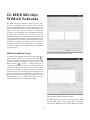
3. Topology Editor
Mode 3: Run Simulation. In this mode, a user can
run/pause/continue/stop/abort/disconnect/reconnect/submit
a simulation in this mode. No simulation settings can be
changed in this mode.
uilding a network topology is the first step toward
running a simulation. It can be easily done through
the use of the topology editor of NCTUns. This
chapter will show you how to quickly build a network
topology by using the topology editor.
B
Mode 4: Play Back. After a simulation is finished, the .ptr
packet animation trace file will be automatically sent back to
the GUI program. The GUI program will then automatically
enter into this mode. In this mode, the user can
play/pause/continue/stop the packet transfer animation.
Four Operating Modes
The (
) buttons on the tool bar correspond to these four different modes, respectively. If a user
needs to switch the operating mode very often among these
modes, it will be more convenient to click one of these
buttons to switch into that chosen mode. At any given time,
one of these buttons will be displayed in blue color. This
reminds the user of the current mode. When a simulation is
running, all of these buttons will be temporarily disabled.
They will be automatically enabled when the simulation is
finished, stopped, or aborted.
Menu->File->Operating Mode->(Draw Topology, Edit Property, Run simulation, Play Back)
Adding Nodes with the Tool Bar
NCTUns has four operating modes. A user needs to switch
the mode at proper times to make the topology editor work
correctly.
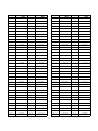
The tool bar contains many types of network device icons,
including host
, hub
, router
, switch
,
802.11(b) wireless LAN (WLAN) access point
,
802.11(b) WLAN ad-hoc mode mobile node
, 802.11(b)
WLAN infrastructure mode mobile node
, 802.11(a)
wireless LAN (WLAN) access point
, 802.11(a) WLAN
ad-hoc mode mobile node
, 802.11(a) WLAN infrastructure mode mobile node
, multi-interface mobile
node (having one 802.11(a) WLAN ad-hoc mode interface,
one 802.11(a) WLAN infrastructure mode interface, one
802.11(b) WLAN ad-hoc mode interface, one 802.11(b)
WLAN infrastructure mode interface, one 802.11(p) OBU,
one GPRS radio, one DVB-RCST satellite interface, and one
802.16(e) mobile station)
, obstacle (can block/attenuate
wireless signal, block mobile node’s movement, and block
mobile node’s view)
, Wide Area Network (WAN)
abstraction
, host subnet
, and five emulationrelated types of network device icons -- external host
,
external WLAN ad-hoc mode mobile node
, external
WLAN infrastructure mode mobile node
, external router
, and virtual router
. As one sees, the icons of most
emulation-related nodes contain an “E”, which reminds that
these nodes represent external real-life nodes used in an
emulation case. The icon of the virtual router contains a “V,”
which indicates that it can represent a real router or be virtu-
Mode 1: Draw Topology. In this mode, a user can add new
nodes/links or delete nodes/links to construct a network
topology. If the moving path of a mobile node needs to be
specified before the simulation starts, this path specification
job must be done in this mode. Note that for the mobile nodes
in the active and tactic mobile ad hoc networks and the
mobile cars in the Intelligent Transportation Systems (ITS),
their moving paths are not specified before the simulation
starts but rather are dynamically changed during simulation.
More information about these two types of networks (i.e.,
Tactic and ITS) will be discussed in later chapters.
Mode 2: Edit Property. In this mode, a user can edit the
property of a node. For example, he (she) can specify which
protocol modules should be used inside a node and what
values should be used for the parameters needed by these
modules. A user can also specify the application programs
that should be run up on a node during simulation. However,
in this mode a user can no longer change the topology of the
network that has been fixed in Mode 1.
19
The network device icons for DVB-RCST satellite networks
include DVB-RCST service provider
, DVB-RCST
Network Control Center (NCC)
, DVB-RCST Return
Channel Satellite Terminal (RCST)
, DVB-RCST feeder
, DVB-RCST traffic gateway
, DVB-RCST satellite
, and DVB-RCST pseudo switch
. The functions of
these devices will be explained in a later chapter for DVBRCST satellite networks.
alized by either a layer-2 switch or a direct Ethernet link.
More information on emulation can be found in later
chapters.
Other network device icons include QoS DiffServ network’s
boundary router
, QoS DiffServ network’s interior
router
, GPRS network’s GGSN device
, GPRS
network’s SGSN device
, GPRS network’s base station
, GPRS network’s phone (radio)
, GPRS network’s
pseudo switch
, optical network’s circuit switch
,
optical network’s burst switch
, optical network’s
protection ring creation tool
,optical network’s edge
router-to-edge router’s shortest (light) path creation tool
,
802.11(b) dual-radio mesh OSPF (using the OSPF routing
protocol) access point
, 802.11(b) dual-radio mesh STP
(using the Spanning Tree Protocol) access point
,
802.11(b) dual-radio mesh multi-gateway switch
,
802.11(e) WLAN infrastructure mode mobile node
, and
802.11(e) WLAN access point
.
The icons for wireless vehicular networks in Intelligent
Transportation Systems are divided into two groups. The
first group is for constructing a road network and includes
ITS road segment
, ITS crossroad
, and ITS road
merger
, ITS Road-Side Unit (RSU) with an 802.11(p)
interface
. The second group is about ITS cars that run on
a constructed road network, which includes ITS car with an
802.11(b) infrastructure mode interface
, ITS car with an
802.11(b) ad-hoc mode interface
, ITS car with a GPRS
radio
, ITS car with a DVB-RCST satellite interface
,
ITS car with an 802.16 (e) interface
, ITS OBU with an
802.11(p) interface (agent-controlled)
, ITS OBU with an
802.11(p) interface (module-controlled)
, and ITS car
with all of the above different interfaces
. The functions
of these icons will be explained in a later chapter for ITS
wireless vehicular networks.
The network device icons for IEEE 802.16(d) WiMAX
networks are classified into two groups. The first group is for
the PMP mode and includes 802.16(d) Base Station (BS) in
PMP mode
, 802.16(d) Gateway Subscriber Station (SS)
in PMP mode
, and 802.16(d) Host Subscriber Station in
PMP mode
. The second group is for the mesh mode and
includes 802.16(d) Base Station in mesh mode
,
802.16(d) Gateway Subscriber Station in mesh mode
,
and 802.16(d) Host Subscriber Station in mesh mode
.
The functions of these devices will be explained in a later
chapter for IEEE 802.16(d) WiMAX networks.
A user can choose a device by clicking the mouse’s left
button on its icon on the tool bar. He (she) then moves the
mouse cursor to a location in the working area and then
clicks again to place the chosen device at the current position
of the cursor.
The network device icons for IEEE 802.16(e) WiMAX
networks include 802.16(e) Base Station (BS) in PMP mode
, 802.16(e) Mobile Station (MS) in PMP mode
. The
functions of these devices will be explained in a later chapter
for IEEE 802.16(e) WiMAX networks.
A network topology consists of not only nodes but also links
between them. Links can be added to the network topology
easily. A user can click the link icon
, move the cursor
to one device node, click the device node to fix one end of
the link, drag the link to another device node, and then
release the mouse button to fix the other end of the link. The
user will see that a straight line between the two selected
nodes is created. The following figure shows the network
topology after the user has placed several links in the
working area to connect these nodes together.
The network device icons for IEEE 802.16(j) WiMAX
networks are classified into two groups. The first group is for
the transparent mode, including 802.16(j) MR_BS in transparent mode
, 802.16(j) fixed RS in transparent mode
, and 802.16(j) MS in transparent mode
. The second
group is for the non-transparent mode, including 802.16(j)
MR_BS in non-transparent mode
, 802.16(j) fixed RS in
non-transparent mode
, and 802.16(j) MS in non-transparent mode
. The functions of these devices will be
explained in a later chapter for IEEE 802.16(j) relay
WiMAX networks.
20
shown on the screen. Note that the information shown for a
layer-1 port (e.g., a hub port) or layer-2 port (e.g., a switch
port) contains only the port ID information. This is because
such ports do not have IP addresses assigned to them.
In a real-world network environment, a mobile node may
move. A mobile node may be an IEEE 802.11(a) WLAN adhoc mode mobile node, an IEEE 802.11(a) WLAN infrastructure mode mobile node, an IEEE 802.11(b) WLAN adhoc mode mobile node, an IEEE 802.11(b) WLAN infrastructure mode mobile node, an multi-interface mobile node,
external WLAN ad-hoc mode mobile node (for emulation
purposes), and external WLAN infrastructure mode mobile
node (for emulation purposes), a GPRS phone, an 802.11(e)
WLAN infrastructure mode mobile node, a 802.16(e) mobile
station (MS), a DVB-RCST Return Channel Satellite
Terminal (RCST), or an 802.11(p) On-Board Unit (OBU).
To specify the moving path of such a node, a user first selects
the moving path tool icon
on the tool bar. He (she) then
clicks the mobile node and start dragging and clicking the
mouse’s left button repeatedly to construct the whole moving
path. This operation continues until the user clicks the
mouse’s right button. Note that for an ITS OBU (i.e., a car),
its moving path is dynamically determined during simulation
rather than be specified before simulation.
When nodes and links are added to or deleted from a network
topology, a node’s ID and the ID of its ports (interfaces) will
be automatically assigned and adjusted by the GUI program.
The GUI program will re-number each node’s ID when any
node is deleted from the topology to make sure that node IDs
are continuously numbered. For a node, when one of its link
is deleted, the GUI program will also re-number the IDs of
all of its ports (interfaces) to make sure that port IDs always
start at 1 and are continuously numbered on a node.
To see where a mobile node has moved to during an
animation playback, a node’s ID is displayed next to its icon
at all times on the screen. A port (interface) of a fixednetwork node is represented by a blue box. For wireless
interfaces such as those used by WLAN mobile nodes,
WLAN access points, GPRS phones, and GPRS base
stations, they are represented by the wireless signal propagation waves
, which indicates the used antenna and it’s
direction. By default, the used antenna is an omni-directional
antenna. In this case, the antenna icon is shown as 360degree circles. If a 3db-beamwidth 60-degree directional
antenna
is used, only 60 degrees out of 360 degrees of
the above antenna icon will be shown and its pointing
direction is the pointing direction of the directional antenna.
A 3db-beamwidth 120-degree directional antenna
is
displayed in the similar way. More information about directional antennas will be discussed in a later chapter.
A moving path is composed of a sequence of turning points
and segments. After a moving path is constructed, any of its
turning points can be easily moved by the mouse to any place
to adjust the shape of the path. Each turning point is represented by a grey dashed square box and contains the (X-loc,
Y-loc, arrival time, pause time, moving speed to the next
point) information. This information can be changed by
double-clicking the box in the “Edit Property” mode.
Suppose that a user wants to change the location of a turning
point, he (she) can click the mouse’s left button on the box,
hold it, and then drag it to any place. When a mobile node is
moving from one point to the next point (i.e., moving on a
segment), its moving speed is fixed. If a user moves the icon
of a mobile node rather than one of its turning point boxes,
its whole moving path will be moved.
When the user switches the mode to the “Edit Property”
mode, the GUI program will automatically generate and
assign an IP and MAC addresses to each port (interface) of a
layer-3 device (e.g., a host or a router). In this mode, if the
user moves the mouse cursor and place it over the interface
(either a blue box or an antenna icon) for a while, the port’s
information (i.e., its port ID and assigned IP address) will be
21
After an arrow is added, a user can move it in three different
ways. First, the user can use the “select” tool to just move the
head of the arrow. Second, the user can use the “select” tool
to just move the tail of the arrow. Third, the user can move
the entire arrow by clicking the mouse’s left button on the
middle of the arrow, holding the button, and then dragging
the mouse. To change the color and width of an arrow, a user
can use the “select” tool to double-click any part of the
arrow. The following figure shows an example network
where labels and arrows are added to make the network more
readable.
There are several other tools on the tool bar. They are select
, delete
, label
, arrow
, undo
, ruler
, zoom in
, zoom out
, zoom into an area
,
view the whole field
, set the zoom scale factor to 1
,
specify physical-layer and channel model parameter
,
and protractor: measure the angle between a specified line
segment and the horizon
.
The “select” function is the most basic operation. If a user
wants to move a device icon, he (she) must select this tool
first. He (she) then presses the mouse’s left button on the
device icon, holds it, and then drags it to the desired place. In
addition, if a user wants to configure a device in the working
area, he (she) should use the “select” tool to double-click it.
The “delete” function can delete a touched node and all the
links connected to it.
The “undo” function can undo the last “delete” operation. It
is a useful function because human sometimes make
mistakes and it may take much time and effort to recover
from a mistake. For example, if a user mistakenly deletes a
router that has 20 links each connecting to a host, the router
and these 20 links will be deleted. To recover from this
mistake without using the “undo” tool, the user will need to
add back a router and then add back 20 links. This tedious
task can be easily done by immediately executing the “undo”
function after the “delete” operation. Note that to undo a
“delete” operation, there should be no other operation
performed between the “delete” and the “undo” operations.
Otherwise, the “undo” function will be disabled by the GUI.
An example network in which labels and arrows are used
The operation of the ruler is the same as creating a link
between two device nodes. A message box will show up
displaying the distance (in meter) between the two selected
nodes. It is primarily used to place WLAN mobile nodes,
WLAN access points, GPRS phones and base stations,
WiMAX subscriber stations and base stations, etc. at proper
locations so that their wireless signals purposely can or
cannot reach each other as planned.
The “label” tool allows a user to enter a label (i.e.,
annotation) such as “Cisco 8100 router” into the network
topology. The user can set the color, font, font style, and font
size of the label before a label is added. After a label is
added, the user can use the “select” tool to move it to any
desired place (e.g., next to a router icon) or change its
attributes by double-clicking it. Adding labels to a network
topology can make it more readable.
Several zoom in or zoom out tool buttons are provided to
allow the user to see the network topology in a suitable view.
The functions of some of these buttons are also provided as
commands located in Menu->View. After choosing the
“Zoom in to an area” tool, a user can use the mouse to select
a rectangular region and zoom into it. Selecting an area is
done by clicking the mouse’s left button, hold it, drag it to the
diagonal corner of the area, and then release it. Normally,
after seeing the details of an area, a user may want the zoom
scale factor to return to the default value of 1. This operation
can be done by using the “Set the zoom scale factor to 1” tool
button. If a zoom scale factor other than 1 needs to be set, a
The “arrow” tool allows a user to add an arrow into the
network topology. Adding an arrow point to a device icon
can highlight the pointed device. Normally, an arrow is
accompanied by a label to describe the pointed device. An
arrow is added in the same way as a link. The user clicks and
holds the mouse’s left button on one place to fix the tail of
the arrow. Then he (she) drags the mouse to the desired
position and then releases the mouse button to fix the head of
the arrow.
22
The “Form wireless subnet” (
) tool is necessary for
various wireless networks, including IEEE 802.11(a/b)
infrastructure mode and ad hoc mode wireless networks,
IEEE 802.16(d) WiMAX wireless networks, DVB-RCS
satellite networks, GPRS networks, etc. The detailed operations for these wireless networks will be illustrated in later
chapters.
user can execute the Menu -> View -> Set Zoom Scale
Factor command. The following figure shows the dialog
box of this function.
Form a Wireless Subnet
The “Form wireless subnet” (
) tool is a very important
tool for setting up simulation cases of wireless networks.
Recall that to save the GUI user’s time and effort, the GUI
program automatically identifies subnets and assigns IP and
MAC addresses to layer-3 interfaces. The GUI program
performs this job very well on a wired network because all
nodes (including host, switch, hub, router, etc.) on such a
network are connected and therefore all subnets on such a
network can be identified. However, for a wireless network
where mobile nodes are isolated nodes, the GUI program
does not have the intelligence to know which mobile nodes
and IEEE 802.11(a/b) access points should belong to the
same subnet. Without such information, because the GUI
program cannot determine the ID of the subnet to which a
mobile node should belong, the GUI program cannot
automatically assign an IP (1.0.subnetID.hostNum) and
MAC address to the mobile nodes.
Form an ITS Car Group
The “Form ITS cars group” (
) tool is used for a user to
group several ITS cars into a fleet, which is called a car
group in NCTUns. The cars in the same group will sequentially follow the route taken by the head car of the group
during simulation. Forming a car group in NCTUns is easy.
One first left-clicks the icon of this tool on the GUI tool
panel. He (she) then left-clicks all the icons of cars in the
working area that are chosen to form the same car group. To
end the selection of cars, one can right-click the mouse and
a dialog box showing the IDs of the chosen cars will pop up.
To solve this problem, the GUI program provides the “Form
wireless subnet” (
) tool for the user to manually group
related wireless mobile nodes together to form a subnet. To
do so, the user first selects this tool and then uses the mouse’s
left button to sequentially click all required nodes. When all
required nodes have been selected, the user clicks the
mouse’s right button to end the selection process. The user
must use this tool to select all required nodes to form a
subnet. For example, for an IEEE 802.11(b) infrastructure
mode wireless network, the user must select all relevant
mobile nodes and access points to form a subnet. The
following figure shows an example usage of this tool. For
this network, the user should use this tool to select the three
mobile nodes and the two access points to form a subnet.
With this information, now the GUI program knows that the
three mobile nodes all reside on the subnet where the access
points reside. As such, the IP and MAC addresses of these
mobile nodes can be assigned automatically.
One should note that the first car that is chosen during the
selection procedure will be automatically designated as the
head car (leading car). Selecting cars into a car group should
conform to the following rules.
23
First, the cars that are chosen to form the same car group
must be on the same road. More specifically, all of them must
be on the same road between two turns. Second, they must
be selected beginning with the head car from left to right or
from right to left without jumping back and forth. Once a car
group is formed, each of them will try to follow the route
taken by its preceeding car during simulation. This feature is
useful for studying inter-vehicle communication among the
cars in a car group.
To manage the created car groups, one can perform the
“Manage ITS cars group” tool, which is at “Menu ->
N_Tools -> ITS Network -> Manage ITS cars group.”
This command provides an interface to view the information
of a car group and delete a car group, which is shown in the
following figure.
A group of nodes can be selected.
Editing the Attribute of Nodes
After nodes are added, a user can enter the “Edit Property”
mode to set the detailed attributes of any node by doubleclicking its icon. Several attributes and functions such as
[Application], [Down Time], and [Command Console] are
provided for many kinds of devices (see the following host
dialog box). Therefore, we present their usages here.
Under the [Application] tab, a user can specify which application program should be run on this node. He (she) can put
the command string into the “command” field. In addition to
the command string, the start time, stop time, and argument
of the specified program can also be set. After an entry is
added, the user can use the “Modify” button to modify the
entry or use the “Delete” button to delete that entry. The
“Add RTP” and “Modify RTP” buttons are for RTP simulations. They will be explained in a later chapter specific to
RTP. The following shows the popped-up dialog box after
the “Add” button is pressed.
Selecting a Group of Nodes
To save time and effort, a user can select a group of nodes
and then apply an operation to all of them. The operations
that can be applied to a group of nodes include (1) move and
(2) delete.
Using the select tool, a user can select a single node by
clicking the mouse’s left button on the node. To select
multiple nodes, the user can hold the “Ctrl” key while
clicking these nodes. Another method is to use the select tool
to draw a rectangle area to select all nodes in that area. To
draw a rectangle area, when the select tool is used, the user
can click the mouse’s left button on one point, hold the
button, and then drag it to another point. The following
figure shows a possible selection result.
If the application program needs to read a configuration file
when it is executed, the absolute file path and file name of its
configuration file must also be entered with all other information. Otherwise, the GUI program will not have the intelligence to also move the needed configuration file to the
remote (or local) simulation server machine. Specifying the
absolute file path and file name is best done via the “browse”
function in the dialog box of the “Add” command.
For example, suppose that when the stg application program
is executed, it wants to read in a configuration file named
trace.cfg and this file is located in /usr/local/testuser. Then
To facilitate selecting a large number of nodes of the same
kind, several commands are provided in the Edit command
menu for various types of networks.
24
node’s interfaces. This is because the PHY (or WPHY)
modules are the right place to disable or enable the transmission and reception of packets. The dialog box of the Phy
module is shown below.
The dialog box of hosts
the entered command string should be something like “stg -i
trace.cfg ...” and the “Input file name” field should be
“/usr/local/testuser/trace.cfg,” which can be completed by
using the “browse” function.
The PHY module in the node editor.
Note that the purpose of providing the absolute file path and
file name in the “Input file name” field is for the GUI
program to successfully locate it and transfer it to the
simulation server machine. On the simulation server
machine, the transferred file is placed in the same directory
as all other simulation description files such as *.tcl.
Therefore, the absolute file path of this file (e.g.,
/usr/local/test.cfg) should not be given in the command
string as an argument to the application. Rather, only its file
name (i.e., test.cfg) should be given in the command string.
To enable the down time setting of an interface, a user needs
to open the node’s node editor, double-click that interface’s
physical-layer module (PHY, WPHY, AWPHY or
OPT_PHY), and make sure that the “Link Failure” option is
checked. If that option is not properly checked, an interface’s
down time periods that come from either a node or a link will
not take effect during simulation. To see the current down
time setting for the interface, the user can click the “See
Down Time Setting” button.
For example, the command string should not be something
like “stg -i /usr/local/testuser/trace.cfg ...”. This is because
the GUI machine and the simulation machine may be
different machines and use different file systems. An
absolute file path used in the GUI machine may refer to
nothing on the simulation machine. Since the simulation
engine will store the specified configuration file in the
working directory of this simulation case, which is also the
working directory of all forked application programs for this
case, the file name given to the application program can be
and should be the file name only without any path specification.
A user can also set the down time periods of a link. By
double-clicking a link, a link property dialog box will show
up. In the dialog box, a user can set the link’s bandwidth,
signal propagation delay, bit-error-rate (BER), and down
time periods for each direction of the link. If the link is an
optical link with multiple channels, the same dialog box can
be used to set the property of each channel. The following
figure shows the property dialog box of an optical link.
The “C.T.A.C” button stands for “Copy To All Channels (of
this selected link).” This function is enabled only when the
user is specifying the property of a channel of an optical link.
(When double-clicking an optical link, the GUI will first ask
the user which channel of the link he (she) wants to
configure.) Clicking this button will copy a field’s current
value to the same fields of all channels of the selected link.
As for the [Down time] tab, a user can set the intervals
during which the node is down (cannot send and receive any
packet). The down time periods specified here will be propagated and set in the PHY (or WPHY) modules of all of the
25
Individually invoking the node editors of the two nodes that
connect to a link to set their link attributes is less intuitive
and may result in inconsistent settings.
[Command console] button is provided in the dialog boxes
of several nodes. This function is enabled only when a
simulation is running. A user can use this console to log into
the current node (the node whose dialog box is shown right
now). A xterm terminal window will appear. In this terminal
window, a user can run the tcpdump program to capture
packets passing through one of this node’s interface or
launch application programs on this node at run time. The
following figure shows a command console usage in which
a tcpdump is capturing packets.
The link property dialog box.
However, the same fields of the channels of all other links
will not be affected. This button can save a user a lot of time
when the user wants to change the property of all channels of
an optical link to a specific setting.
The “C.T.A.L” button stands for “Copy To All Links (and to
all of their channels).” Clicking this button will copy a field’s
current value to the same fields of all links (and to all of their
channels if they are optical links) in the simulated network.
This button can save a user a lot of time. For example, if a
user wants to set the bandwidth of all links to 20 Mbps, he
(she) can open up any link’s property dialog box, change the
bandwidth from 10 to 20 Mbps, and then click the “C.T.A.L”
button next to the Bandwidth field. The bandwidth of all
links (and their channels if they have any) in the simulated
network will be changed to 20 Mbps.
Since links are bidirectional, a user can separately specify
the down time periods for each direction of a link. The down
time periods specified for a direction of a link (say, from
node A to node B) are automatically propagated to and set in
the physical-layer module (e.g., PHY) of node A. Therefore,
the down time periods set in an interface’s physical-layer
module actually is the union of the down time periods of the
node to which this interface attaches and the down time
periods of the link to which this interface connects.
A command console can be invoked during a simulation. In this
case, a tcpdump is capturing packets in this command console.
For a router, suppose that the user wants to capture the
packets flowing through one of its interfaces. Further assume
that this particular interface is assigned 1.0.2.3 IP address.
The user can first execute “ifconfig -a” command to find out
the information about all of the router’s interfaces. From the
output, the user can find the name of the desired interface
which is assigned 1.0.2.3. In NCTUns, an interface’s name is
in the ethXXX format, where XXX is the interface’s port ID.
After finding the name of the desired interface, the user can
execute the following command “tcpdump -i ethXXX” to
launch the tcpdump program. Since the launched tcmdump
is the real-life tcpdump program, all tcpdump options are
supported. This means that the user can use any packet
filtering rule such as “tcpdump -i eth2 src 1.0.2.1” or
“tcpdump -i eth3 -w tdump.log dst port 8002.”
In addition to the down time information, other attributes of
a link are also automatically propagated to the appropriate
modules of the two nodes that connect to this link. For
example, the bandwidth, signal propagation delay, and BER
are all propagated to and set in the corresponding physicallayer modules. Note that this automatic link parameter
propagation process will override the settings specified by
the user in the node editor for these physical-layer modules.
The GUI program adopts this design because it is more
intuitive to set a link’s attributes by double-clicking it.
26
The command console is a very useful function. A user can
use this console to launch application programs at run time
to generate traffic. For example, while the simulation is
running, the user can open a receiving node’s command
console to launch the “rtcp -p 8000” TCP receiving program
and then open a sending node’s command console to launch
the “stcp -p 8000 1.0.1.2” TCP sending program, assuming
here that the receiving node has an interface assigned 1.0.1.2
IP address.
•
Host
In addition, executing the ping command in a command
console is very useful. Doing so can help a user find out
whether the routing path between two nodes has been
correctly set up during simulation.
The simulation engine of NCTUns is a discrete-event
simulation engine. Thus, its simulation clock may advance
faster than the real-world clock. To allow the user to take his
(her) time to type commands in a command console, it is
suggested that the speed of the simulation is set to “As fast
as the real-world clock,” which can be done in Menu ->
G_Setting -> Simulation -> [Speed tab] rather than the
default “As fast as possible.”
The “Mobile IP” tab is related to the Mobile IP protocol.
NCTUns supports the Mobile IP protocol; including both the
basic scheme and the advanced route optimization (RO)
scheme. The types of nodes involved in Mobile IP are host
(correspondent host), mobile node (infrastructure mode),
and routers (where the home agent or the foreign agent is
running). As such, all of these types of nodes have the
“Mobile IP” tab. More details about how to run Mobile IP
will be discussed in a later chapter.
To quit a command console, a user can use the mouse to kill
the xterm window. All command consoles will be automatically killed by the GUI program when the simulation is
finished, stopped, aborted, or disconnected.
Note that an output file generated by an application program
invoked in a command console will be transferred back to
the simulation case’s XXX.results directory on the GUI
machine. For example, the tdump.log generated by the
previous “tcpdump -i eth3 -w tdump.log dst port 8002”
command will be transferred and stored in the case’s
XXX.results directory.
The “Add RTP” and “Modify RTP” buttons are for RTP,
RTCP, and SDP protocols. A user can use “Add RTP” to
specify the various parameters given to a RTP application
program. Like the “Modify” button, the “Modify RTP”
button is used to modify a command string generated by a
previous “Add RTP” operation. The “Delete” button is a
general-purpose button and can be used to delete a RTP or
non-RTP application entry. More information about how to
run RTP will be discussed in a later chapter.
In addition to the above shared tabs, each device may have
its own ones. We present them below.
27
•
Because every port of a hub must use the same bandwidth,
one has to specify the link bandwidth used by the ports of the
hub in the Bandwidth field.
External Host, Mobile Nodes, and Router
•
In this dialog box, a user can specify whether all routers in a
case should run routing daemons (e.g., RIP, OSPF) to
construct their routing tables or their routing tables should be
calculated in advance by the GUI program. Run-time routing
table content lookup can be performed by clicking the
“Show routing table” button when a simulation is running.
An external host, external mobile node (ad-hoc mode),
external mobile node (infrastructure mode), or external
router represents a real device in the real world. They are
used for emulation purposes. Because emulation is an
important function, a separate chapter titled “Emulation” is
dedicated to it. Explanations of the usage of these fields will
be documented in detail in that chapter.
•
Router
•
Hub
28
Switch
•
Access Point
•
Mobile Node (Ad-hoc and Infrastructure mode)
Under the [AP Property] tab, a user can set the down time
periods for an access point.
A powerful and flexible configuration dialog box is provided
for WLAN mobile nodes. Under the [Path] tab, the moving
speed, location (X, Y) of each turning waypoint, pause time
during which a mobile node stays at the current waypoint can
be configured.
To insert a waypoint into the middle of the existing path, the
user can first use the mouse to click the appropriate insertion
point in the path dialog box and then click the “Generate”
button. In addition, the moving speed between the new point
and the next point will be automatically calculated so that the
next point’s arrival time need not be changed.
To generate a random waypoint path, several methods are
provided. A user can ask the GUI program to generate
random waypoints on the fly; either one point at a time or ask
it to keep generating waypoints until the arrival time of the
last waypoint exceeds the specified time. A user can also
import a mobile node’s path from an existing *.mpt file.
Each line in an mpt file represents a waypoint and its format
is (X_pos, Y_pos, Arrival Time, Pause Time, Moving
Speed). This file may be generated by a program (e.g., a
vehicle microscopic traffic simulator) or as a result of
Under the [Wireless Interface] tab, a user can examine the
interface’s attributes (e.g., the used frequency channel and
the wireless signal transmission range).
29
executes the Menu ->File ->Save As command to save the
current case into another one. (3) In the new case, the user
invokes any mobile node’s node editor to replace protocol
module A by protocol module B in that node’s protocol
stack. (4). The user uses the “C.P.A.N.S.T.” button to
replace the parameter values (including the protocol stacks)
of all other mobile nodes with the new one. (5) Finally, the
user runs the new simulation case and obtains the performance results of protocol module B under the same network
topology and configuration.
exporting a mobile node’s moving path. In the topology
editor, a user can also drag-and-drop the mouse to directly
place a path’s waypoints.
Under the [Single-hop connectivity] tab, the GUI program
will calculate and show at what time this mobile node
can/cannot reach other mobile nodes in its single-hop transmission range.
On the other hand, under the [Multi-hop connectivity] tab,
the GUI program will calculate and show at what time this
mobile node can/cannot reach other mobile nodes via
multiple hops, through the help of the ad-doc mode
forwarding.
Note that the above task can also be easily done by executing
Menu -> G_Tools ->Export Mobile Nodes and Their
Paths to File and Menu -> G_Tools -> Import Mobile
Nodes and Their Paths from File commands and Menu ->
G_Tools -> Import Network Traffic Application File
command. Detailed instructions on these commands will be
presented later in this chapter.
These two functions are provided for comparing research
results with the ideal results. The outputs of these two
functions represent the most accurate and ideal routing paths
that only “God” can know and achieve at any time. These
two functions are meaningful only when the used wireless
module is the simple WPHY, which has a specific transmission range and is not very realistic. When the used
wireless module is the advanced AWPHY, which does not
have a clear transmission range but is more realistic, the two
connectivity functions are not very meaningful.
•
WAN (Wide Area Network Abstraction)
Under the [Interface] tab, a user can examine the interface’s
attributes (e.g., the used frequency channel and the wireless
signal transmission range).
The “C.P.A.N.S.T.” button stands for “Copy the Parameters
to All Nodes of the Same Type.” If a user executes this
function, the parameters used by this WLAN mobile node
will be copied to all WLAN mobile nodes with the same
operating mode (i.e., ad-hoc or infrastructure). That is, the
parameter values of all other WLAN mobile nodes with the
same operating mode will be replaced by the current one. For
example, if the current WLAN mobile node is an ad-hoc
mode mobile node, its parameter values will be copied to
(and only copied to) all other ad-hoc mode mobile nodes.
A WAN is a layer-2 node that simulates various properties of
a Wide-Area-Network. It can purposely delay, drop, and/or
reorder passing packets according to a specified distribution.
Inside the simulation engine, a WAN is implemented as a
layer-2 switch with only two ports. The packet dropping,
delaying, and reordering functions are achieved via the
WAN module used inside a WAN node. In a WAN node, a
WAN module exists in each of its two ports. It delays, drops,
and/or reorders the port’s outgoing packets. The forward and
backward packets of a flow that traverse a WAN can
therefore receive different treatments.
The “C.P.A.N.S.T.” is a useful function. Suppose that a user
wants to compare the performances of two different routing
protocols (A and B), he (she) may attempt to test the performances of these two protocol modules under the same
network topology and configuration. That is, the initial
locations and the moving paths of all mobile nodes in these
two cases should be exactly the same; the difference should
be only in the used protocol stack.
With this function, this task can be easily done in the
following steps. (1) The user first tests the performance of
protocol module A in a simulation case. (2) The user
30
Other methods to add Mobile Nodes
In addition to the simple way by which a GUI user clicks the
mouse to add one mobile node at one time, there are several
other methods that can be used to add multiple mobile nodes
in just one step.
Insert Multiple Mobile Nodes
A user can insert multiple mobile nodes using the same
protocol stack and parameter settings by executing just one
command. Each kind of wireless networks (e.g., IEEE
802.11(a/b) WLAN, IEEE 802.11(e) WLAN, IEEE
802.16(d/e/j) WiMAX, GPRS, DVB-RCS satellite network,
etc.) provides its own command for this purpose and these
commands are located in Menu-> N_Tools. The following
figure shows the dialog box of this command for IEEE
802.11(b) WLAN networks. The added mobile nodes can be
placed at random positions or in an M * N array. Their
operating mode (ad hoc or infrastructure) can also be chosen.
The user can generate a large number of WLAN mobile
nodes that use a protocol stack other than the default one. To
do so, the user can first invoke the node editor in this dialog
box to specify the protocol stack used by these mobile nodes.
If this operation is not done before adding a large number of
nodes, the user later may suffer from invoking all mobile
nodes’ node editors to configure their protocol stacks
individually. Fortunately, with the mobile node’s
“C.P.A.N.S.T.” function, this tedious task can be easily and
quickly done.
A WAN module exists in each port of a WAN node. The WAN
module can purposely delay/drop/reorder its port’s outgoing
packets.
Inside the parameter dialog box of the WAN module, packet
delaying, dropping, and reordering function can be independently used. Supported distributions include constant,
uniform, exponential, and normal distributions. The
following figure shows the dialog box of the WAN module.
The parameter dialog box of the WAN module.
The dialog box of the “Insert WLAN Mobile Nodes” command.
31
After importing a mdt file, the user can further use the
“Background Graph” function of NCTUns to paste the used
highway or city map onto the background of the topology
editor. (This function will be presented later in this chapter)
With a background map, when the simulation is executing or
when the playback is going on, the user will see vehicles
move on highways or roads on the map and vehicles
wirelessly exchange their packets via other vehicles. This
will give the user a global view of wireless transmission
activities on a highway or in a city.
Import/Export Mobile Nodes and Their Paths from/to File
These two commands are located in the Menu -> G_Tools
menu. The import function loads all mobile nodes and their
moving paths from a *.mdt file while the export function
saves the same information into a mdt file.
It’s convenient and useful for a user to save mobile nodes’
moving paths to a file and later reload and reuse them. For
example, to compare the relative performance of several
mobile ad-hoc network (MANET) routing protocols under
the same moving pattern, the user can (1) create a simulation
case in which mobile nodes move in a desired pattern, (2)
export these mobile nodes and their moving paths to a mdt
file, (3) create a new simulation case for studying the performance of a different routing protocol, (4) import the same
mdt file in each of these simulation case, and (5) use the
“Node Editor” button in the dialog box of a mobile node to
use the desired routing protocol module, (6) use the
C.P.S.T.A.N button to replace the parameter values
(including the protocol stacks) of all other mobile nodes with
this one, (7) finally, run the new simulation case and obtains
the performance results of the different routing protocol
under the same network topology and configuration.
Generate Random Waypoints
The Menu -> G_Tools -> Generate Random Waypoints
for Mobile Nodes command can be executed to generate
random waypoints for all WLAN mobile nodes. There are
two ways of doing this job. The first one is to generate the
next waypoint randomly for all mobile nodes. When the user
clicks the button, one more random waypoint will be
generated for every mobile node. The user can press the
button continuously to continuously generate more random
waypoints. The other way is to automatically generate
random waypoints until the arrival time of the last waypoint
exceeds the specified time. The following figure shows the
dialog box of this function.
The format of the mdt file is simple and explained in the file
itself. A user can first export the moving paths of a case to a
mdt file and then see its content. The import function is very
useful for large-scale simulation cases where the number of
mobile nodes is very large and the lengths of their moving
paths are very long. In such a situation, the mobile nodes’
locations and their moving paths may better be generated by
a script program, which will save the user a lot of time and
effort.
This facility is also very useful for using a special mobility
pattern that is not supported by NCTUns. Right now,
NCTUns can only automatically generate random waypoints paths for mobile nodes or allow a user to manually
specify the moving paths of mobile nodes. However, in some
cases, a user may want to study a mobile network with a
different mobility pattern.
Remove All Moving Paths
Executing this function will delete all mobile nodes’ moving
paths. This will give the user a clean working area to start
with. This function is located in Menu -> G_Tools ->
Remove All Moving Paths of Mobile Nodes.
For example, when using NCTUns to study ITS (intelligent
transportation systems) problems, we can first use a microscopic vehicle traffic simulator (e.g., VISSIM) to generate
more realistic moving paths of vehicles moving on a
highway or in a city. (Note: VISSIM considers the carfollowing and lane-changing driver’s behavior.) A user can
write a simple program to convert the moving path log file
generated by a third-party program (e.g., in this case,
VISSIM) to a mdt file and then import it into the GUI.
Import Network Traffic Application File
For a large network that has hundreds or thousands of nodes,
double-clicking the icon of each of these nodes to enter the
application command string for the node is a tedious and
time-consuming job. To avoid wasting time and effort on
doing this job, the user can use the Menu -> G_Tools ->
32
Show Moving Path
Import Network Traffic Application File command to
read in a traffic configuration file (.tfc). The format of a .tfc
file is exactly the same as the .tfc file exported by the GUI
program for a simulation case when it switches its mode to
“Run Simulation.” Therefore, to understand the format of a
.tfc file, the user can first make a simple case and then export
the case’s .tfc file. Each line in the .tfc file specifies the node
ID, starting time, ending time, and application command
string for a node. The format of a line is $node_(nodeID)
start_time end_time application_command_string.
This command can change a flag to display or not to display
the moving paths of WLAN mobile nodes.
Show Icon
This command can change a flag to display or not to display
the mobile node icons. It is useful when the user just wants
to see mobile nodes’ current locations (represented by boxes
with solid and thick edges) and does not want them to be
messed up with their initial locations (represented by mobile
node icons). Not showing the initial locations of mobile
nodes in the working area can make the current network
topology clearer.
Normally, a .tfc file imported by the “Import Network
Traffic Application File” command is generated by a script
or a program written by the user. Each traffic generator (i.e.,
application program) command string specified in the .tfc
file will be put into the Applications tab of the specified
node. This facility can save a user a lot time because now the
user need not invoke each node’s dialog box individually to
enter its used application command strings.
Show ID
This command can change a flag to display or not to display
the IDs of mobile nodes. Like other display flags, in a large
simulation case, not showing the IDs of mobile nodes may
make the current network topology clearer.
Remove All Network Traffic Application
Settings for Optical Networks
The Menu -> G_Tools -> Remove Network Traffic Applications command does the reverse job. It removes the application command strings of all nodes from their respective
Applications tabs. These two commands are useful for largenetwork cases because they can save much time and effort
for a user. The following figure shows where these two
commands are located.
The following commands can be executed to change the
settings of optical networks. They are located in Menu ->
N_Setting -> Optical Network.
Set Optical Link Wavelength Channel Number
In a WDM optical network, an optical link usually have
multiple channels using different wavelengths. In NCTUns,
all optical links in a WDM optical network must have the
same number of channels. This command sets the number of
channels per optical link. The default number is 3. If a user
wants to use a different number, he (she) must execute this
command to change the setting before adding any optical
link to the topology editor. Executing this command after an
optical link is added is not allowed.
Settings for WLAN Mobile Nodes
Set Optical Link Packet Playback Channel(s)
Several display flags are provided for WLAN mobile nodes
in Menu -> N_Setting -> 802.11(b) Wireless Network.
Like a packet transfer animation played on a fixed network,
packets transmitted on an optical network can be played to
show their movements on optical links. Since a WDM
optical link has multiple channels and a user may be inter33
ested in seeing packets flowing on only one, several, or all
channels of a link, this command is provided for a user to
select which channels’ packets should be displayed.
Set Optical Link Packet Playback Color
Like the channel color settings for packet playback on
WLAN and GPRS networks, this command is provided to
set the color scheme for packet playback over different
channels of a WDM optical link.
Set Maximum OBS Control Packet Processing Time
The usage of this parameter for optical-burst-switching
networks will be explained in a later chapter about optical
networks.
Setting the Background Graph
Sometimes placing a background graph on the network
topology working area can provide a great value. For
example, when a user studies how to place wireless access
points or base stations in a city to achieve the optimal performance/utilization/coverage, it is much better if the user can
place the city map on the working area as the background
graph. Commands related to the background graph function
are located in Menu -> G_Setting -> Background Graph.
Paste Background Graph
This command selects a .bmp file and pastes it as the
background graph.
In the following, we use an ITS (Intelligent Transportation
Systems) simulation case as an example and paste a map of
the HsinChu city in Taiwan on the working area.
Position Background Graph
Scale Background Graph
After pasting the background graph, the user can place the
graph at any place (i.e., shift its top-left corner by an offset
vector) on the working area and specify its scaling factor
(i.e., enlarge it or shrink it).
This command can scale the background graph in a different
way. Sometimes it is more convenient than the scaling
function provided in the dialog box of the above “Position
Background Graph” command.
34
After executing this command, the user will automatically
enter the “background graph scaling” mode. In this mode,
like using the ruler function, the user can drag and drop the
mouse over a line. A dialog box will pop up asking the user
how long (in meters) the line corresponds to in the real
world.
For example, on the bottom-right corner of the map there is
a scale saying that this small segment corresponds to 891
meters in the real world. With this information, the user can
drag and drop the mouse over this segment and input 891
into the dialog box. Usually after scaling the map to get the
1:1 ratio, the background graph will become very huge and
thus only a very small part of it can be shown on the screen.
The user can use the “view the whole field” tool button to
view the whole background graph.
Using an ITS (Intelligent Transportation System) case as an
example, now the user can import mobile nodes and their
moving paths from a file. In this ITS case, each mobile node
represents a mobile car and its moving path represents how
it moves on the roads. This command is located in Menu ->
G_Tools.
Import Network Traffic Application File
Suppose that we would like to run some application
programs on these imported mobile cars to exchange information among them, we can use this command to import
application program command strings from a .tfc file. The
details of this command have been explained before.
Executing this command can save the user a lot of time
because he (she) need not invoke the GUI dialog box of
every mobile car to specify their application programs. This
command is located in Menu -> G_Tools.
Set Background Graph Brightness
Obstacles
Normally the user will place the icons of network nodes on
top of the background graph. To achieve a better visual
quality, it is better to brighten the background graph a bit.
This command allows the user to adjust the brightness of the
background graph in a fine-grain way.
In the real world, not all fields are open space for wireless
signal. Some may have high mountains or tall buildings
blocking wireless signal’s propagation or attenuating their
power. In some researches, we may want to purposely add
obstacles to the open field to block/attenuate wireless signal
at some places in the field. In NCTUns, an obstacle
is a
rectangle that can block a mobile node’s view, block a
mobile node’s movement, or completely block wireless
signal or just attenuate the power of wireless signal. These
properties are important for simulating tactical mobile ad
hoc networks. An obstacle can be added in the same way like
adding an arrow. With obstacles, a user can simulate a more
complicated and interesting field setting. This can facilitate
testing wireless network and protocol performances (e.g.,
handoff) under a more realistic field setting.
After a series of operations, now the background graph is
properly set. When a user saves a simulation case, the current
background graph settings will be saved to the file as well.
Therefore, next time when the user re-opens the simulation
case file (.tpl), the background graph will automatically be
set up without the user’s help.
Import Mobile Nodes and Their Paths from File
35
An obstacle can block node’s view, node’s movement, or wireless
signal. Wireless signal can just be attenuated rather than being
totally blocked.
Communication between the two mobile nodes is affected by the
obstacle located in the middle of them.
obstacles with different property, he (she) can use the above
command again to change the default property of an
obstacle.
Note that the single-hop connectivity and multi-hop connectivity calculations provided in a mobile node’s dialog box
take into account the existence of obstacles. In addition, the
God routing daemon for WLAN ad-hoc mode mobile nodes
takes into account the existence of obstacles as well. The
name of the file that describes the obstacles in a simulation
case is XXX.obs.
Generate Large Networks
To generate a large network topology, it is tedious for a
network researcher to add nodes and links to the topology
editor one at a time. NCTUns provides a convenient tool for
a user to automatically generate a large network whose
structure is similar to that of the Internet. A user can execute
the Menu -> G_Tools -> Generate Large Internet-like
Network command to specify the parameters of the large
network to be generated.
If a user clicks and holds on one side of an obstacle, a yellow
square box will appear at that side and he (she) can rotate or
extend the obstacle. Another side of the obstacle is the fixed
point of the rotation or extension operations. If a user clicks
on the middle part of an obstacle, a yellow square box will
appear at both sides and he (she) can move the selected
obstacle to any place.
In the parameter dialog box, the “Node Number” field
specifies the number of nodes of the network to be generated.
This number cannot be too small. Otherwise, the generated
topology will not share the same properties with the Internet
topology. Links in the generated network are classified into
three different categories and each category can use a
different bandwidth. These categories are the core, edge, and
LAN links, respectively. The unit of bandwidth in this dialog
box is Mbps.
If a user double-clicks an obstacle, a property dialog box will
pop up. A user can specify the obstacle's properties such as
its width, whether it should block mobile nodes’ view,
whether it should block mobile nodes’ movement, and
whether it should block wireless signal or just attenuate the
power of the signal.
Sometimes a user may want all obstacles to have the same
property that is different from the default property. It is
tedious to change the property of each obstacle one by one
after every obstacle is placed. Therefore, a user is suggested
to change the default property of an obstacle before placing
any obstacle by using the Menu -> G_Setting -> Obstacle
command. After this operation, all obstacles added will have
the new default property. If the user needs to place more
The “Max X” and “Max Y” fields specify the length and
width of the field over which the generated network will be
laid. Their default values are taken from the simulation
case’s field sizes, which can be configured in Menu ->
G_Setting -> Simulation. Each node in the generated
topology will be placed on the field according to their
generated (x, y) locations. The signal propagation delay of a
36
File manipulations
link between two nodes will be automatically calculated and
set. It is the distance between these two nodes divided by the
light speed.
Several commands are provided to manipulate files. They
are located in Menu -> File.
New
Executing this command will close the current simulation
case and clear the working area for a new case.
Open
Reload an already existing case. The .tpl file of the desired
case should be selected to open the case.
Save
Save the current simulation case’s topology and node configurations into the .tpl and .tcl file, respectively. This case can
later be reloaded.
Save as
Save the current simulation case’s topology and node configurations into a new file suite. The name of the case shown on
the screen is changed from the current case name to the new
case name.
Subnet
To quickly expand a simple network topology, a user can
choose the subnet
function on the tool bar and then
click on the working area to insert a group of hosts. The
group of added hosts are all connected to a switch. When the
subnet dialog box appears, a user can enter the desired
number of hosts and the desired subnet radius. The following
figure shows the subnet dialog box.
Print to File
Capture the network topology area shown on the screen and
save it to a .bmp file. The captured graph can later be sent to
a printer for printing or be included in a technical report for
illustration.
Background Job Management
Any background job submitted to the dispatcher can be
manipulated here. They can be deleted, stopped, aborted, or
retrieved. The following figure shows the dialog box of this
function.
37
Simulation
The “Refresh” button is used to update the information
shown in this table. Each time the user clicks this button, the
GUI program will retrieve the most up-to-date information
about each background job from the dispatcher.
The command for setting the various global parameters of
the current simulation case is located in Menu -> G_Setting
-> Simulation.
Under the [Simulation] tab, the total simulation time in
virtual time and the maximum of X, Y, Z coordinates can be
specified. Currently the maximum time that can be simulated
is 4,200 seconds in virtual time. The user can select whether
the .ptr file (packet transfer trace) should be generated or not.
The user can further select which types of network’s packet
transfers should be logged into the ptr file.
Setting the Simulation
Dispatcher
The command for setting the dispatcher used for the current
simulation case is located in Menu-> G_Setting ->
Dispatcher.
The random number seed given to the simulation engine for
this simulation case can also be specified. Using the default
value of 0 indicates to the simulation engine that it can
choose a random number for the random number seed. That
is, each time the same simulation case is run, a different
random number seed will be used. If the random number
seed is fixed to a value greater than 0, NCTUns can generate
repeatable results for each run of the same simulation case.
This dialog box asks a user to provide the IP address and port
number used by the dispatcher. The GUI user’s login account
and password for using the remote (can be local) simulation
server should also be provided here. It is VERY important
that the account name of the GUI user used on the local GUI
machine and that used on the remote (can be local)
simulation server should be exactly the same. Otherwise, the
network simulator cannot work correctly. For the singlemachine mode, the user name specified here MUST be the
same user account name by which the user logs into this local
machine. Otherwise, the simulation cannot run correctly. For
security concerns, the “root” account is not allowed and thus
is blocked here by the GUI.
If the user is using the single-machine mode, the IP address
entered here can be 127.0.0.1 (the IP address of the loopback
interface lo0). The port number entered here must be the
same as the CLIENT_PORT specified in the dispatcher.cfg
Under the [Speed] tab, the tick time can be specified. The
default setting is that one tick represents 100 nanoseconds in
virtual time in a simulation. This setting can be changed to a
38
movement during a simulation, the option “Display packet
transmission and node movement during simulation” has to
be chosen.
smaller value such as 10, or 1 nanosecond, which is useful
for generating more accurate results on high-speed networks
(e.g., with more than 1 Gbps bandwidth links).
The speed of the simulation engine can be set to “As fast as
possible” or “As fast as the real-world clock.” Normally, a
user would want a simulation case to be finished as soon as
possible. However, when NCTUns is turned into an emulator
or the user conducts a human-in-the-loop tactical mobile ad
hoc network simulation, the speed of the simulation engine
should be set to “As fast as the real-world clock.” This option
is also useful when a user wants to use the command console
during a simulation. The following figure shows the dialog
box of the speed tab.
Under the [GUI] tab, the ratio of meter/pixel can be
specified. Changing this setting to a larger value (e.g., 100)
is useful for a network whose size is physically very large
(e.g., the backbone network of USA, see the following
figure).
Under the [Real Time] tab, two GUI display options for
military tactical mobile ad hoc network (MANET)
simulation can be specified. In general MANET simulation
cases, each mobile node's moving path is pre-specified
before the simulation is started. In contrast, in military
tactical MANET simulation cases or Intelligent Transportation Systems simulation cases mobile nodes' moving paths
are dynamically generated by agent programs running on
mobile nodes during simulation. To allow such type of
simulations, the option “Dynamic moving path generation
during simulation” must be chosen. In addition, if a user
wants to see the display of packet transmission and node
If a network is physically very large and nodes need to be placed at
their correct positions on a map with the correct physical distances
between them, it is better to use a larger value for the meter/pixel
ratio parameter so that node icons can still be seen with the whole
39
GetAll {module} {tag}
Using a large value can allow the whole network to be
clearly shown on the screen without using the “Zoom Out”
function. Although the user can use the default value (i.e., 1)
and the “Zoom Out” function to display the whole network
topology on the screen, node icons will become too tiny to be
seen on the screen and it will be very difficult for the user to
manipulate these tiny icons (e.g., to select them).
Under the [System command] tab, to-be-executed system
commands and their output file names can be specified here.
A system command is a command that, when executed, will
get or set an object’s value at the specified time. The output
of the command will be saved to the specified output file,
which will later be transferred back to the GUI program
when the simulation is finished.
Note that a tag is a string associated with a particular variable
declared and used in a protocol module. A variable here can
be a single-value variable (e.g., a FIFO queue’s maximum
queue length) or a multi-column multi-row table (e.g., a
switch table that has multiple [IP address, MAC address]
mapping entries). It is the protocol module developer’s job to
write a command() method in his (her) module to recognize
a tag and then get/set the value of its associated variable.
In addition to getting/setting a single object’s value, the
values of all objects of the same kind can be get or set at the
same time to take a global snapshot of the whole network.
For example, this function can be used to take the snapshot
of the current routing tables of all routers. This global
snapshot information can help a researcher study the convergence of a protocol.
Time: the starting time for executing this command
Command: the system command string
Output file name: the name of the output file
The system commands provided by NCTUns are listed
below. Their syntax and meanings are also explained below.
Set: set a value to a variable in a module
Set {node} {port} {module} {tag} {value}
Get: get the value of a variable from a module
Get {node} {port} {module} {tag}
GetAll: like Get, but get the values of the requested variable
from the same modules used in all ports of all nodes
40
View Messages from Simulation Engine
More information about the get/set command can be found
in “The Protocol Developer Manual.for the NCTUns 6.0
Network Simulator and Emulator”
NCTUns provides a runtime messaging mechanism to
enable protocol modules to dynamically send messages to
the GUI program during simulation. In the Run Simulation
mode, when the GUI program receives a message from a
protocol module, it will pop up a window to show the
received message. The following figure shows a snapshot of
the popped-up window.
Running the simulation
Several commands are provided to control the execution of
simulation cases. They are located in Menu -> Simulation.
Run, Pause, Continue, Stop, Abort
After a user switches to the “Run Simulation” mode, the user
can start running the simulation by executing the “Run”
command in this group.
After the simulation is completed, one can use the command
“Menu -> G_Tools -> View Messages from Simulation
Engine” to review the messages issued by protocol modules
in the Play Back mode. The snapshot of this tool is shown
below.
During simulation, the user can use the “Pause,” “Continue,”
“Stop,” and “Abort” commands to pause, continue, stop, and
abort the simulation. The difference between the “Stop” and
“Abort” commands is that the former command will return
the current simulation results to the GUI program while the
latter command will not.
Reconnect, Disconnect
A user can disconnect the GUI from a currently-running
simulation job. Doing this allows him (her) to quit the GUI
program and switch to do other things. The user can come
back later, restart the GUI program, and then reconnect to the
disconnected simulation job.
Submit as Background Job
A user can directly submit a simulation job as a background
job to the dispatcher for execution. Its effect is the same as
first running up the simulation and then immediately disconnecting the GUI from the just launched simulation job. To
reconnect to a currently running background job or retrieve
results from a finished background job, the user should use
the Menu -> File -> Background Job Management
command.
To dynamically transmit messages to the GUI program, a
protocol module has to use specific message-passing APIs
provided by the simulation engine instead of using traditional message-printing library calls, such as printf(). More
information about these APIs is explained in the “The
Protocol Developer Manual for the NCTUns 6.0 Network
Simulator and Emulator.”
41
View Packet Trace
It is useful to view the packet trace file in a human understandable way. Viewing this file can help a researcher debug
a network or a protocol. To do so, a user can execute Menu
-> G_Tools -> View Packet Trace to open the desired .ptr
file. The binary .ptr file will be converted to text by the
“printPtr” tool automatically and shown in the popped up
window. The text is shown by the “more” program, which
supports vi-like search commands.
Set the Frequency of Updating Mobile Node Routing Paths
(for the GOD Module)
This Menu -> G_Tools -> Set the Frequency of Updating
Mobile Node Routing Paths (for the God Module)
command controls how frequently the routing paths should
be recomputed for the GOD routing module. A higher
frequency allows the GOD routing module to respond to link
failures more quickly but at the cost of generating a larger
file to store more information.
Show Packet Trace Format
This Menu -> G_Tools -> Show Packet Trace Format
command shows and explains the format of the output
generated by the Menu -> G_Tools -> View Packet Trace
command. The following figure shows the result of
executing this command.
Summary
The topology editor provides users with a friendly and easyto-use working environment. In this environment, a user can
quickly build network topologies and specify application
programs. Executing and controlling simulations can also be
easily done in this environment.
Display All Node and Link Down Time
A user may set down times for nodes and links to test how
network protocols would respond to these down times. For
WDM optical links, down times can also be set for each
individual WDM channel. This Menu -> G_Tools ->
Display All Node and Link Down Times command
displays the down times specified for all nodes and links in
the simulated network. A user can execute this command to
have a global view of the down times specified for the whole
simulated network.
42
4. Node Editor
he node editor provides a convenient environment
for a user to flexibly configure the protocol modules
used inside a network node. By using this tool, a
user can easily add, delete, or replace a module with his (her)
own module to test the performance of a new protocol.
T
Protocol Module Concept
A protocol module implements a particular protocol such as
ARP or a particular function such as the FIFO packet scheduling discipline. In the node editor, all modules that are
grouped in the same module group (displayed at the top of
the node editor) share similar properties. For example, in the
802.11 MAC group, we may have one module called
“802.11MAC” while having another one called
“my802.11MAC.”
NCTUns provides several pre-developed protocol modules.
Users can add new protocol modules to the node editor or
replace some existing modules with his (her) own ones. For
example, in the PSBM (packet scheduling and buffer
management) module group, four modules (FIFO, RandomEarly-Detection, Deficit-Round-Robin, WAN) are currently
supported. A user may add a new PSBM module such as a
RIO module to it.
The node editor’s screen layout.
group buttons. Because only four modules can be shown at
the same time, the user can use the “<<” and “>>” buttons to
see other modules not shown on the screen.
In the middle working area, the protocol modules used by
this node are shown. Here, a chain of protocol modules
represent the protocol stack used by a port (interface). The
user can use the mouse to easily add, delete, or replace
protocol modules in the working area.
Detailed information on how to add a new protocol module
to both the simulation engine and the node editor is
documented in “The Protocol Developer Manual for the
NCTUns 6.0 Network Simulator and Emulator.”
At the bottom are several control buttons. The “Cancel”
button discards all changes that have been made to this
node’s protocol modules. The “OK” button accepts all of the
changes made so far. The “Undo” button removes the effect
of the last delete operation. (Note: only the LAST delete
operation can be undone.) The “Redraw” button re-layouts
the protocol modules so that they look nice when shown on
the screen. (This is particular useful after a user performs the
insert or delete operation.)
Screen Layout Explanation
In the following, we will briefly explain the screen layout of
the node editor. To see the node editor, in the topology editor
a user first switches the mode to the “Edit Property” mode by
executing the Menu -> File -> Operating Mode -> Edit
Property command. Then the user can double-click a node
that he (she) wants to edit. After the node’s dialog box shows
up, the user can click the “Node editor” button to invoke the
node editor to edit that node’s protocol stack.
The Copy-To-All-Port (CTAP) button copies the values of
the currently selected module’s parameters to the same
modules in all ports of this node The Copy-To-All-Node
(CTAN) button does the similar job. However, it copies the
values to the same modules in all ports of all nodes in the
whole simulated network.
At the top of the node editor are various module groups. The
protocol modules that share the same role in a protocol stack
are grouped together under the same group name. When the
user clicks one module group button, all modules belonging
to that module group will be shown right below the module
43
connects to this node will be shown at the bottom of the node
editor. This information can help the user distinguish interfaces when remote nodes are of the same type.
The “X” button means “delete.” After clicking this button,
now the node editor’s mode enters the “delete” mode. From
now on, whenever the user uses the mouse to left-click a
module or a link, that object will be deleted. The “Arrow”
button means “select.” After clicking this button, now the
node editor’s mode enters the “select” mode. From now on,
the user can move a protocol module to any desired place.
The user can also choose a module from a module group,
insert, and place it in the middle working area.
The protocol stacks of a node can have two levels. In WDM
optical network simulations, not just each interface needs a
protocol stack; instead, each WDM channel of an interface
needs a protocol stack. Therefore, a two-level protocol stack
may be displayed in the node editor for WDM nodes. The
protocol modules at the first level are relevant to an interface
while the protocol modules at the second level under an
interface are relevant to a WDM channel of that interface.
The following figure shows an example.
In the node editor, a chain of protocol modules represents the
protocol stack used for an interface. As such, if a router has
two interfaces, it will have two module chains. For example,
if a router has one interface that connects it to a host and has
another interface that connects it to a switch, it will have two
protocol chains shown in its node editor. The following
figure shows the node editor for this router.
To help a user distinguishes which module chain is for which
interface, the icon of the remote node that an interface
connects to (through a link) is shown at the bottom of that
interface. As such, in the figure, a green switch icon and a
grey host icon are placed at the bottoms of the two interfaces,
respectively.
Add, Delete, and Replace a Module
Here we use an example to illustrate how to replace a FIFO
module with a RED module.
If the remote nodes that a node connects to are all of the same
type (e.g., suppose that in the above example the router
connects to two hosts), showing the remote nodes’ icons at
the bottom does not help distinguish interfaces. In this case,
the user can position the mouse cursor over a remote node
icon in the node editor. The node ID of the selected remote
node and the ID of the port on that remote node which
44
Step 1: We first invoke the node editor of a router so that its
initial protocol module chain is shown as follows.
Step 3: Then we select the “X” tool button and click the
mouse on the FIFO module to delete it. The result is shown
below.
Step 4: Then we link the RED module with the ARP and
MAC802.3 modules together. To link together two modules,
a user performs the same operation as he (she) does when
creating a link between two nodes in the topology editor. At
the top and bottom of a module, there is a small box. A link
must start and end on these small boxes. After linking up
these modules, the result is shown below.
Step 2: Then we choose the RED module from the top and
place it in the middle working area. The resulting screen is
shown below.
45
Add a New Module to the NCTUns
Step 5. Since the job is finished, now we redraw the node
editor to make it look beautiful. The result is shown below.
After a user has developed his (her) own module, two tasks
must be done to integrate the new module into the NCTUns.
The first task is to introduce the new module to the node
editor so that it can appear in an appropriate module group
and its parameter dialog box can be shown when it is doubleclicked in the middle working area. The second task is to
register the new module with the simulation engine so that its
code is executed when a simulation case using the new
module is executed.
Add a New Module to the Node Editor
To let the node editor know that a new module has been
added to it, the user must add and place the definition of the
module into the module description file (mdf.cfg). To understand the detailed format and meanings of the module
description file, readers should refer to that file stored in
/usr/local/nctuns/etc and “The Protocol Developer Manual
for the NCTUns 6.0 Network Simulator and Emulator.”
Register a New Module with the Simulation Engine
To let the simulation engine find the code of the new module
and successfully execute it, the user must also register the
module code with the simulation engine.
NCTUns provides a simple method for a user to register a
new module with the simulation engine. Detailed procedures
are documented in the “The Protocol Developer Manual for
the NCTUns 6.0 Network Simulator and Emulator.”
Step 6. If we would like to keep the changes made so far, we
can click the “OK” button. On the other hand, if we would
like to discard all changes that we have made so far, we can
click the “Cancel” button.
Set or View Module Parameter Values
Summary
To set or view the values of a module’s parameters, a user
can double-click a module in the middle working area and
then its module parameter dialog box will appear. The
following figure shows the parameter dialog box of the FIFO
module.
In this chapter, we present the concept of protocol modules
and the node editor. The node editor is an environment in
which a user can flexibly configure the protocol stack and
parameter values used inside a node. NCTUns provides
some pre-built protocol modules. A user can easily add his
(her) own protocol module to the node editor to test its
performance.
46
5. Packet Animation
Player
General Options for Packet Animation
fter a simulation execution is finished, the generated
simulation results will be automatically transferred
back to the GUI program and then saved in the
user’s local hard disk. Suppose that the simulation case’s
topology file is named “test.tpl.” Then the name of the
resulting packet animation trace file will be “test.ptr.” Later
on, when the user wants to do post analyses about the
simulation results, he (she) can use the “Packet Animation
player” to play back the animation. This is a very useful
feature for both education and research purposes.
A
During the play of a packet animation trace, a user can
change some options of the GUI program to suit his (her)
needs. These options are described below.
Time Bar
The time bar shows the packet animation progress in a time
interval, which is called a time window here. A user can drag
the time knot to any desired time. Two buttons are provided
to change the size of the time window by a factor of 10. That
is, the time window size can be either increased 10 times
larger or decreased 10 times smaller. A user can conveniently perform this job by left-clicking the “zoom-out”
button (
) or the “zoom-in” (
) button.
Reloading Simulation Results
To watch a previously generated packet animation trace, a
user should first open its corresponding topology file.
Menu -> File -> Open
Time bar and its knot
Right below the time bar, a red vertical line indicates that a
wired packet transmission starts at this time, a green vertical
line indicates that a wireless LAN packet transmission starts
at this time, and a blue vertical line indicates that a GPRS
packet transmission starts at this time. Note that because the
ending times of packet transmissions are not depicted here,
it may be difficult for a user to move the time knot to the time
when a packet transmission exactly ends. Therefore, these
vertical lines are depicted here for reference purposes only.
The GUI program purposely ignores WLAN broadcast
packets and does not plot vertical bars for them on the time
bar. This is because a WLAN access point broadcast its
beacon frame every 0.1 seconds and plotting these broadcast
packets on the time bar will de-focus the user’s attention on
important packets generated by application programs.
The user then switches to the “Play Back” mode directly. The
GUI program will then automatically reload the simulation
results (including the packet animation trace file). Since the
animation file is usually very large, this process may take a
while. To give the user an idea of the progress, a progress bar
is shown during the loading process.
To know exactly when a packet transmission starts and ends,
a user can use the printPtr utility program to first convert the
binary animation trace file into a text file and then search it
in the file.
After the packet animation trace file is loaded, the user can
left-click the start button (
) of the time bar located at the
bottom. The player will start playing back the logged packet
transfer animation.
Animation playing buttons
47
The default value for this parameter is 100%. Other values
such as 200% and 50% are provided. If the ratio of the
selected value to the default value is X, the used time
advancement quantity will be X times of the default time
quantity.
Animation playing buttons are provided to alter playing
sequences. They can be executed by left-clicking their corresponding buttons.
(
) plays the animation. If a user clicks it while the
animation player is idle, the player will start to play the
packet animation trace. If a user clicks it while the animation
player is already running, the time knot will jump directly to
the nearest future time where there is a packet transmission.
This feature is very useful when the traffic is sparse.
(
) pauses the animation.
(
) stops the animation.
If the playback clock is not advancing, the time knot can be
dragged to any location to jump directly to a desired time.
The following figure shows the time bar.
(
) moves the animation time window by one time
window size in the backward direction.
If the user knows the exact time where the playback clock
should directly jump to, he (she) can double-click the clock
display area at the left to enter the time. The unit of the
entered time should be in tick and the relationship between a
tick and its duration in virtual time is specified in Menu ->
G_Setting -> Simulation’s [Speed] tab. This function is
particularly useful when the user has used the “printPtr”
utility program to read the ptr packet trace file and wants to
jump the clock directly to a specific time to see the packet
transfer activities occurring at that moment. The following
shows the dialog box of this function.
(
) moves the animation time window by one time
window size in the forward direction.
The 40fps (frames-per-sec) selection box controls the
display quality of the animation. It defines how many frames
should be played in a second in the real time. Using a smaller
value can increase the animation speed because fewer CPU
cycles are needed to refresh the screen. However, the
resulting animation may become rigid and not smooth.
The 100% selection box controls the progress of the
animation. It affects the time advancement quantity of the
playback clock. During playback, the playback clock is
advanced by a fixed time quantum in each of the playback
loop. After the playback clock is advanced, all of the packet
transfers whose transmission period (i.e., the period between
the transmitting and receiving times) covers the current
playback clock time are selected to be displayed on the
screen. Choosing a larger value for this parameter will
advance the progress of the animation playback more
quickly. However, more packet transfers will be skipped and
not displayed in the animation playback. Therefore, if packet
transmission times over the links in a simulated network are
tiny (e.g., tiny 58-byte TCP ACK packets transmitted on a 10
Mbps link or 1500-byte TCP data packets transmitted on a 1
Gbps link), it is better to use a smaller value for this
parameter to see them.
Animation Effects
Wired network and wireless network have different characteristics. Therefore, we demonstrate their corresponding
animation effects separately.
Wired Network
We use two screen shots to illustrate and explain wired
network packet animation.
48
segment length on a particular link is determined by the
transmission time of that packet on that link relative to the
signal propagation delay of the link.
Wireless LAN Network
Similarly, in the following, two screen shots are presented to
illustrate and explain the wireless animation effects.
Successful packet transmissions
Wireless packet transmissions (IEEE 802.11 DATA frame)
Packet drop & collision (represented by cross)
•
A link is painted in yellow color if there is any packet
flowing on it.
•
A packet is depicted by a segment with an arrow (for
brevity, it will be called an “arrow” in the following
description.).
•
A collided packet is depicted by an arrow with a cross on it.
•
During a packet transfer, if a link is painted in red, it means
that this link is an intermediate link for this packet. In
contrast, if this link is painted in yellow, it means that one
end of this link is the real source or destination node of the
packet.
•
Wireless transmission (IEEE 802.11 ACK frame)
•
The arrow length is determined by the packet’s length.
Therefore, a user can expect that the arrow length is
proportional to the packet length. In fact, a packet’s
49
Two concentric circles are centered at a transmitting node.
The smaller circle stands for the “transmission range”
while the larger one stands for the “interference range.”
Within the interference range, a station can sense the
existence of other nodes’ signals. However, only when the
receiving station is within the transmission range of the
sending node, will the packets be guaranteed to reach the
receiving station successfully.
•
An IEEE 802.11 (b) data frame is depicted by an arrow
with a “DATA” annotation.
•
An IEEE 802.11 (b) acknowledgement packet is depicted
by an arrow with an “ACK” annotation.
Summary
This chapter presents the “Packet Animation Player”
capability of the GUI program. In this chapter, relevant
options are covered. In addition, both wired and wireless
packet animation effects are illustrated and explained.
50
6. Performance
Monitor
Operations on the Performance Monitor
Several other commands are provided in the menu of the
performance monitor window. In the following, we will
explain their usages.
erformance monitor is a generous-purpose and
useful tool that can graphically display plots of
performance metrics. For example, it can help users
monitor a links’ utilization or a TCP connection’s achieved
throughput. This chapter gives an overview of the functions
provided by the performance monitor.
P
PM.Menu -> File
Running the Performance Monitor
A user can execute the Menu -> G_Tools -> Plot Graph
command to launch the performance monitor. The following
figure shows the window of the performance monitor.
New
When a user executes this command, a new graph window
will be opened. Up to six graph windows can be shown on
the screen at the same time.
From the performance monitor (PM) window, a user can
execute the PM.Menu -> File -> Open command to select a
desired log file to open.
The user can then left-click the start icon (
) of the time
bar at the bottom of the screen. As the packet animation
proceeds, the performance monitor window will display the
corresponding performance curves over time. Note that the
performance monitor can be used as an independent tool
without the animation player running. That is, it can read a
log file generated by any other application program as long
as the log file uses the two-column (X, Y) format.
Open
A user can execute this command to open a desired log file
as a graph window's data source file. The specified log file
will be associated with the graph window. Normally, log files
are generated by the simulation engine if the user selected to
do so in some protocol modules (e.g., 802.3 or 802.11
modules) in the node editor. However, they can also be
generated by application programs running on nodes such as
rtg.
51
Quit
A user can execute this command to quit the current graph
window.
PM.Menu ->Window
The example01.8023_N2_P1_InOutThrput.log is a log file
generated by the simulation engine and can be plotted by the
Add/Remove Graph
This command provides a sub-menu from which a user can
choose different graph data source files. Selected graph data
source files are headed with check marks. A user can use this
command to display the performance curves of more than
one graph source files in the same window. It is useful for
comparing different performance metrics at the same time.
Snapshot
A user can execute this command to pop up the snapshot
window for capturing the performance curve that is currently
displayed in the window.
PM.Menu ->Color
Several commands are provided under the color sub-menu
for setting the colors of the different parts of the graph
window.
In this window, clicking “Re-snapshot” button will recapture the performance curve that is being displayed.
Clicking “Save” button will save the snapshot as an image
file of the “bmp” type. Clicking “Cancel” will quit the
window.
Snapshot All
Background
A user can execute this command to take snapshots of all
existing graph windows. The feature is very useful for
comparing different performance metrics at the same time.
Executing this command can select a color from the palette
and set it as the background color of the current graph
window.
52
Axis
Executing this command can select a color from the palette
and set it as the color of the X and Y axes of the current graph
window.
Grid
Executing this command can select a color from the palette
and set it as the color of grids of the current graph window.
Graph
This command provides a sub-menu from which a user can
choose a different graph data source file to display its
performance curve. In addition, the user can select a color
from the palette and set it as the color of the performance
curve in the current graph window.
Use Default Settings
Executing this command will use the default colors for the
background, axes, and grids of the current graph window.
PM.Menu ->Option
Width (X-axis):
This field specifies how many seconds’ worth of data should
be displayed in the graph window.
Interval of Grid (X axis):
This field sets the grid interval of the X axis. This value will
be multiplied by 0.1 to derive the interval between two
consecutive grids on X axis.
General Setting
Executing this command can set the various presentation
parameters of a graph window. The following figure shows
the dialog box of this command.
Y label:
This field sets the label of the Y axis.
Range - Y Min:
This field sets the minimum value of the Y axis.
Graph Title:
This field sets the title of the graph.
Range - Y Max:
This field sets the maximum value of the Y axis.
Show Grids in Background:
This field sets whether the grids should be visible.
Interval of Grid (Y axis):
This field sets the grid interval of the Y axis.
X label:
This field sets the label of the X axis.
Performance Curve Style - Line-Points:
Selecting this option specifies that the performance curve
53
should be drawn using straight lines to connect adjacent
points.
Performance Curve Style - State-Transition:
Selecting this option specifies that the performance curve
should be drawn using horizontal lines to connect adjacent
points.
In addition to the above settings, a performance curve’s
legend and color can be easily set by double-clicking the
curve’s legend located at the top-right corner. For example,
a user can double-click the default “graph X” curve legend
to change it.
Global Setting
The performance curve is plotted using the line-point format.
Executing this command can associate a graph data source
file with a log file. Up to six associations can be specified in
this dialog. To select a log file from the local host, a user can
press the “Browse” button.
Graph Mode
The performance curve is plotted using the state-transition format.
Executing this command can control how to display a performance curve. Currently there are two modes. The first mode
is “line points” while the second mode is “state transition.”
The following two screen shots clarify the differences
between these two modes.
Summary
This chapter presents the functions and relevant settings of
the performance monitor. A user can use this tool to analyze
performance results. In addition, a user can easily take
important snapshots of some performance curves to make
reports.
54
7. Emulation
and 4) add some settings on the simulation machine and
external real-world hosts/routers, so that real-world traffic
can be directed to and received from the simulated network.
he NCTUns network simulator can be easily turned
into an emulator. An emulator allows real-world
devices to interact with a simulated network and
forces real-world packets to experience user-specified
network conditions. Emulation is very useful for testing the
functions and performances of real-world devices and
observe how it would perform under various network conditions. In this chapter, we present how to turn NCTUns into
an emulator.
T
To describe the connectivity between an external host/router
and a simulated network (i.e., to specify to which node in the
simulated network the external host/router is attached), each
real-world external host/router is represented as an external
host/router icon in the simulated network. A GUI user can
easily specify to which node in the simulated network an
external host/router should connect by drawing a link
between these two nodes. Like all other links in the
simulated network, such a link has its own properties and is
simulated by NCTUns.
Emulation in NCTUns
To let the packets generated by an external host enter the
simulated network or let an external host receive packets
originated from the simulated network, the external host
must be physically connected to the simulation machine via
some network (which can be as simple as an Ethernet cable).
Ideally, such a network should have infinite bandwidth and
zero latency. Although in the real world such a network does
not exist, for achieving accurate results, the used network
should still have low latency and high bandwidth. For
example, a 100 Mbps Fast Ethernet network may be used for
this purpose. One should notice that, for NCTUns, an
external host must reside on the same subnet as the
simulation machine; otherwise, the emulation function
will not work properly.
NCTUns supports emulations [1]. In an emulation, a realworld host, an ad-hoc mode mobile host, an infrastructure
mode mobile host, or a router can exchange its
TCP/UDP/ICMP packets with any node in a simulated
network. These real-world devices are called external host,
external ad-hoc mode mobile host, external infrastructure
mode mobile host, and external router, respectively. In
addition, NCTUns supports a new node type called “virtual
router,” which is used for conducting distributed emulations
and will be explained separately in another chapter. To
represent them in an emulation network topology, these
devices have their own node icons, which are shown here.
.
In addition to the above usage, two real-world hosts
(including mobile hosts in the following discussion) can
exchange their packets via a simulated network. For
example, a TCP connection can be set up between two realworld hosts with their packets traversing a network
simulated by NCTUns in real time.
NCTUns uses an emulation kernel module to seamlessly
bridge the real-life network and the simulated network. This
kernel module performs the Network Address Translation
(NAT) function: It intercepts incoming/outgoing packets,
properly modifies their IP addresses and port numbers, and
finally injects them into either the simulated network or the
external real-life network according to their destination IP
addresses. The detailed design and implementation information is available in [1].
Emulation provides several advantages. First, real-world
traffic and simulated traffic can interact with each other.
Second, real-world traffic can be subject to user-specified
packet delay, drop, reordering, and packet scheduling and/or
buffer management schemes. With emulation, we can test
the function and performance of a real-world host (actually
the host can be any device with an IP address) and see how
it would perform under various network conditions without
getting, knowing, or modifying its internal protocol stack.
After specifying the emulation topology, the nctunsclient
program will automatically generate the commands required
for setting up the emulation kernel module. Then, when
starting an emulation, the NCTUns simulation engine will
trigger the Linux kernel to properly load and initialize the
emulation kernel module using the specified commands via
system calls. Because the emulation kernel module
consumes some CPU time to perform the required NAT
function, it is recommended to conduct an emulation using a
high-speed machine.
Emulation is achieved by 1) specifying to which node in a
simulated network an external host/router should be
connected; 2) physically connecting the external host/router
to the simulation machine via a network; 3) setting the speed
of the simulation engine to be as fast as the real-world clock;
55
In the following, we illustrate the detailed steps to configure
an emulation case using the GUI program.
The Simulation Speed Setting for Emulation
Once a user adds an external host into the network topology,
the speed of the simulation engine will automatically be set
to the speed of the real-world clock. During the simulation,
the simulation’s simulation clock will then be synchronized
with the real-world clock every 1 ms. Therefore, the
emulation function’s latency precision is 1 ms.
From experimental results, it is found that the precision may
degrade and vary if NCTUns is used in its single-machine
mode. During an emulation, the GUI program, simulation
engine, traffic generator application programs, and some
daemon programs all need to be run on the single machine.
Because they need to compete for the machine’s CPU cycles,
the emulation precision may degrade. However, it has been
found that if NCTUns is used in its multiple-machine mode,
the precision is quite high and does not degrade.
When all external hosts are removed from the network
topology, purposely the GUI is designed not to automatically
switch the speed option back to “As fast as possible.” This is
because even though there is no external host in a network
topology, sometimes it is still useful to let a simulation run at
the speed of the real-world clock. For example, when a GUI
user wants to use the command console function during a
simulation, he (she) may want the simulation to run at the
real-world clock speed. For the same reason, even if a case is
a simulation rather than an emulation, the simulation speed
option can still be set to “As fast as the real-world clock.”
the external host in the simulated network. With the IP
address mapping specified here, the emulation kernel
module will intercept these packets and then forward them to
the external host in the real world.
Insert External Host into a Network Topology
First, a user can click on the external host icon on the tool bar
and add it to the network topology. Second, he (she)
then switches to the “Edit Property” mode and enters the IP
address used by the external host in the real world. This
information must be known by the emulation kernel module
otherwise it cannot forward packets originated from the
simulated network to the external host. In addition to the
above information, the user needs to enter the IP address
used by the simulation machine in the real world.
Direct Traffic to the Simulated Network
The assigned host IP address is the IP address assigned to
this external host in the simulated network. If a node in the
simulated network wants to actively send packets to the
external host, the node can use the external host’s assigned
IP address as these packets’ destination IP addresses. These
packets will then traverse the simulated network and reach
Suppose that in the real world the simulation machine’s IP
address is 10.0.0.1 and the external machine’s IP address is
10.0.0.2 and they are physically connected via a crossover
Ethernet cable. Suppose that the external machine wants to
56
make a TCP connection to a node in the simulated network
whose assigned IP address is 1.0.3.1. Then on the external
machine, the user should first execute the following
FreeBSD command to add the required routing entry to the
system routing table.
route add 1.0/16 10.0.0.1
In the above command, 1.0/16 means that the destination
network address is 1.0.X.X. (16 means that the netmask is
255.25.0). Note that every node in the simulated network is
assigned an IP address of the form of 1.0.X.X. As a result,
the above command indicates that all outgoing packets
whose IP destination address is 1.0.X.X should be first sent
to the gateway whose IP address is 10.0.0.1. In this case,
since 10.0.0.1 is the simulation machine’s IP address, these
packets will be sent to and received by the simulation
machine.
external host to run up the TCP sending program. The
following figure shows this network and traffic configuration.
If the external machine is a Linux machine, the needed
routing command should be as follows:
route add -net 1.0.0.0/16 gw 10.0.0.1
Emulation Examples
In the following, we illustrate how to use external host,
external ad-hoc mode mobile host, external infrastructure
mode mobile host, and external router in emulations.
External Host
External hosts can be connected to a simulated network in
several ways. In the following, we present three emulation
examples.
If the external host is physically connected to the simulation
machine and its routing configuration has been properly set
according to previous explanations, TCP packets will begin
to be exchanged between the simulated host and the external
host. The following figure shows the physical setup for this
emulation case.
Example 1
The following figure shows the first example. In this figure,
an external host is connected to the simulated network via a
simulated link that sits between it and a simulated switch.
The external host wants to exchange TCP packets with the
host in the simulated network. Suppose that the IP address
assigned to the simulated host is 1.0.1.1 and the IP address
assigned to the external host in the simulated network is
1.0.2.1.
Second, suppose that the simulated host wants to make a
greedy TCP connection to the external host. In such a case,
the “rtcp -p 8000” command should be first run up on the
external host waiting for the TCP connection setup request to
come. Then the “stcp -p 8000 1.0.2.1” command can be
entered to the [Application] tab of the simulated host’s
dialog box. Doing so will run up a TCP sending program on
the simulated host during the emulation. When the emulation
starts, TCP packets will begin to be exchanged between the
simulated host and the external host.
First, suppose that the external host wants to make a greedy
TCP connection to the simulated host on the left. In such a
case, the “rtcp -p 8000” command can be entered to the
[Application] tab of the simulated host’s dialog box. Doing
so will run up a TCP receiving program on the simulated host
during the emulation. After starting the emulation, the GUI
user can execute the “stcp -p 8000 1.0.1.1” command on the
57
configurations have been properly set, their TCP packets
will begin to be exchanged via the simulated network. That
is, their TCP packets will traverse the simulated link, switch,
and router.
Example 3
The following figure shows the third example, which is
intended to show that an emulation topology can be very
simple. In this figure, two external hosts are connected to the
simulated network and the simulated network is just a link.
The left external host connects itself to the left end of the link
while the right one connects itself to the right end of the link.
The two external hosts want to exchange their TCP packets
via the simulated link. Assume that the IP address assigned
to the left external host is 1.0.1.1 and the IP address assigned
to the right external host is 1.0.1.2.
Example 2
The following figure shows the second example. In this
figure, two external hosts are connected to the simulated
network. The right external host connects itself to the
simulated switch while the left one connects itself to the
simulated router. The two external hosts want to exchange
their TCP packets via the simulated network. Suppose that
the IP address assigned to the left external host is 1.0.1.1 and
the IP address assigned to the right external host is 1.0.2.1.
Suppose that the left external host wants to make a greedy
TCP connection to the right external host. In such a case, the
“rtcp -p 8000” command should be first run up on the right
external host. Then the GUI user can start running the
emulation. The GUI user can then execute the “stcp -p 8000
1.0.1.2” command on the left external host to run up the TCP
sending program. If the two external hosts are physically
connected to the simulation machine and their routing
configurations have been properly set, their TCP packets
will begin to be exchanged via the simulated network. To
purposely delay, drop, reorder real-life packets while they
are exchanged on the simulated link, a user can put a WAN
node on the link to achieve these effects.
Suppose that the left external host wants to make a greedy
TCP connection to the right external host. In such a case, the
“rtcp -p 8000” command should be first run up on the right
external host. Then the GUI user can start running the
emulation. The GUI user can then execute the “stcp -p 8000
1.0.2.1” command on the left external host to run up the TCP
sending program. If the two external hosts are physically
connected to the simulation machine and their routing
58
External Ad-hoc Mode Mobile Node
802.11(b) wireless interface. Actually, it does not matter
which type of network link is used between the simulation
machine and the external mobile host as long as their IP
packets can be exchanged on the used network media.
For emulation, an external ad-hoc mode mobile node in the
real-world need not be a mobile device (e.g., a notebook
computer equipped with an IEEE 802.11 interface).
Actually, it can be a fixed host which uses a normal Ethernet
link to connect to the simulated network. Because the
external mobile node’s IEEE 802.11 MAC protocol is
simulated in the simulated network, the IEEE 802.11 MAC
protocol on the real-life external mobile node is not used
between the external mobile node and the simulation
machine to exchange their packets. In addition, mobility is
simulated by the simulator rather than by the user physically
moving the external mobile device around the simulation
machine. For these reasons, the external mobile device
actually can be a fixed host.
As in the external host emulation case, the simulation
machine and the external mobile host should be on the same
subnet. Let’s assume that the simulation machine’s IP
address is 10.0.0.1 and the external machine’s IP address is
10.0.0.2 and they are physically connected via a Fast
Ethernet crossover cable. Then on the external mobile host,
the user should first execute the following command to add
the required routing entry to its system routing table.
route add 1.0/16 10.0.0.1 (on FreeBSD)
route add -net 1.0.0.0/16 gw 10.0.0.1 (on Linux)
Also, if a node (either a simulated node or an external mobile
node) wants to send packets to another node (either a
simulated node or an external mobile node), it should use the
IP address assigned to that node in the simulated network.
The following figure shows an emulation example in which
one external ad-hoc mode mobile host communicates with a
simulated mobile host via another simulated mobile host.
Initially, the external mobile host on the left can exchange
packets with the simulated mobile host on the right via the
middle mobile host. However, as time proceeds, the mobile
host on the left begins to move away from the simulated
mobile host (not in the real-world but in the simulated
network) and eventually it will be away from the transmission range of the middle mobile host. At this time, it can
no longer communicate with the simulated mobile host on
the right via the middle mobile host.
In short, the usage of external ad-hoc mode mobile host is the
same as that for external host.
External Infrastructure Mode Mobile Host
The usage of external infrastructure mode mobile host is
every similar to those of external host and external ad-hoc
mode mobile host. The only exception is that in the GUI
dialog box of the external infrastructure mode mobile host,
the user needs to provide the gateway IP address information. This requirement is reasonable as in the GUI dialog
box of a normal infrastructure mode mobile node (in the
[Interface] tab), the user also needs to provide such information.
The following figure shows an emulation example in which
one external infrastructure mode mobile host communicates
with a simulated host via a simulated wireless access point.
Like in the external ad-hoc mode mobile host case, initially
the external infrastructure mode mobile host can communicate with the host at the top. However, as time goes by, it
will eventually leave the coverage area of the wireless access
point and no longer can communicate with that host.
The physical setup and routing configuration for this case is
the same as that used for the external ad-hoc mode mobile
host case.
The physical setup for this emulation case is one simulation
machine and one external mobile host (need not be mobile).
The external mobile host can use either a normal Ethernet
link to connect to the simulation machine or an IEEE
59
packets enter the simulated network, they need to traverse
simulated links and subject to the bandwidth and delay of
these simulated links.
External Router
An external router can also interact with a simulated
network. This is a very useful feature as traffic originated
from the simulated network can be directed to the router,
experience the router’s packet scheduling and buffer
management processing, and then return back to the
simulated network. With this capability, we can easily test
the router’s functionality (e.g., sending virus and networkattack packets to see whether the router can detect them).
The following figure shows an emulation example case
where three simulated hosts are connected to an external
router. On top of this topology, we set up two greedy TCP
connections. The first one starts at host 1 and ends at host 3
while the second one starts at host 2 and ends at host 3. The
packets of these two TCP connections need to pass the
external router. That is, they need to leave the simulated
network (host 1 and host 1), enter the real-world network to
reach the external router, leave the router, and then reenter
into the simulated network (host 3).
The simulation engine needs some information about the
external router. Thus, the user needs to provide some information in an external router’s GUI dialog box, which is
shown below. For each port of the external router in the real
world, the user needs to provide the association among the
following information entities: its assigned IP address in the
simulated network (this information is automatically
provided by the GUI in the second column of this association
table after the port ID column), the real IP address of the
network interface on the simulation machine that connects to
this port via a link, the name (e.g., eth1) of the above
interface (on the simulation machine), and the real IP address
used by this port on the real-world router. The dialog box of
the external router contains an example to illustrate the
settings.
The physical network setup for running this emulation is
shown as follows. The simulation machine needs to have
three network interfaces each of which connects to one port
of the external router. Clearly, three physical links are needed
to connect these network interfaces to these ports -- one to
one. These physical links are correspondingly represented as
links in the simulated network, whose bandwidths and
delays are specified in and simulated by the simulation
machine. As in previous emulation cases, once real-world
60
1) “route add 200.Z.X.Y -interface NICNAME” or “route
add 200.Z.X.Y GatewayIPaddress.” (on FreeBSD)
2) “route add 200.Z.X.Y dev NICNAME” or “route add
200.Z.X.Y gw GatewayIPaddress.” (on Linux)
Here Z is a variable taken from the set of all subnet IDs used
in the simulated network, NICNAME is the name of the
interface on the external router (e.g., fxp0 or eth0), and
GatewayIPaddress is the IP address of the interface on the
simulation machine to which the external router would like
to send packets with 200.Z.X.Y as their destination IP
address.
Note that “200” must be used because the emulation kernel
module changes the destination IP address of a packet (e.g.,
1.0.X.Y) going to the real router to 200.0.X.Y so that the
packet can be recognized by the router and be sent back by
the external router to the simulated network correctly.
Using the emulation network settings depicted in the
following figure as an example, assuming that the interface
names for the 140.113.1.1, 140.113.2.1, and 140.113.3.1 on
the simulation machine are eth1, eth2, and eth3, respectively,
then the association table should contains the following
entries: (1, 1.0.1.2, 140.113.1.1, eth1, 140.113.1.2) for port
1, (2, 1.0.2.2, 140.113.2.1, eth2, 140.113.2.2) for port 2, and
(3, 1.0.3.2, 140.113.3.1, eth3, 140.113.3.2) for port 3.
Beside changing the first number of the destination IP
address from the default “1” to “200,” the emulation kernel
module also changes the second number of the destination IP
address from the default “0” to the ID of the subnet where the
packet leaves the simulated network to enter the external
router. This design is required. Without such a design, if
there are two external routers in a simulated network, when
a packet enters the simulated network after being sent to an
external router and then coming back, the emulation kernel
module will not be able to know from which subnet this
packet should continue its journey over the simulated
network. Suppose that host 2 on the left sends a packet to
host 3 on the right. Then the destination IP address of the
packet will be changed to 200.2.3.1 before being sent to the
external router.
Using the above example to illustrate, suppose that link 1 is
subnet 1, link 2 is subnet 2, and link 3 is subnet 3 in the
simulated network. Further suppose that the IP address of
host 1 is 1.0.1.1, the IP address of host 2 is 1.0.2.1, and the
IP address of host 3 is 1.0.3.1, and the IP address of the
external router on link 1 is 1.0.1.2, the IP address of the
external router on link 2 is 1.0.2.2, and the IP address of the
external router on link3 is 1.0.3.2. Suppose that in the real
world the real IP address used by the external router port
configured with 1.0.1.2 in the simulated network is
140.113.1.2, the real IP address used by the external router
port configured with 1.0.2.2 in the simulated network is
140.113.2.2, and the real IP address used by the external
router port configured with 1.0.3.2 in the simulated network
is 140.113.3.2. Further suppose that on the simulation
machine the IP address of the interface connecting to link1 is
On the external router in the real world, some routing entries
need to be added to its routing table so that packets originated from the simulated network can be redirected back to
the simulated network. The rules for generating these routing
entries are as follows. For every host with 1.0.X.Y as its
assigned IP address in the simulated network, we need to use
the following commands to add the needed routing entries:
61
host routing to specify these routing entries. The following
shows the routing commands for adding these subnet routing
entries:
140.113.1.1 in the real world, the interface connecting to
link2 is 140.113.2.1, and the interface connecting to link3 is
140.113.3.1. These address settings are best viewed by the
above figure.
(On FreeBSD)
For this example case, on the external router we need to
execute the following routing commands to add the required
entries.
route add 200.1.1/24 140.113.1.1
route add 200.2.1/24 140.113.1.1
route add 200.3.1/24 140.113.1.1
(On FreeBSD)
route add 200.1.1.1 140.113.1.1
route add 200.1.2/24 140.113.2.1
route add 200.2.1.1 140.113.1.1
route add 200.2.2/24 140.113.2.1
route add 200.3.1.1 140.113.1.1
route add 200.3.2/24 140.113.2.1
route add 200.1.2.1 140.113.2.1
route add 200.1.3/24 140.113.3.1
route add 200.2.2.1 140.113.2.1
route add 200.2.3/24 140.113.3.1
route add 200.3.2.1 140.113.2.1
route add 200.3.3/24 140.113.3.1
-------------------------------------------------
route add 200.1.3.1 140.113.3.1
(On Linux)
route add 200.2.3.1 140.113.3.1
route add -net 200.1.1/24 gw 140.113.1.1
route add 200.3.3.1 140.113.3.1
route add -net 200.2.1/24 gw 140.113.1.1
-------------------------------------------
route add -net 200.3.1/24 gw 140.113.1.1
(On Linux)
route add 200.1.1.1 gw 140.113.1.1
route add -net 200.1.2/24 gw 140.113.2.1
route add 200.2.1.1 gw 140.113.1.1
route add -net 200.2.2/24 gw 140.113.2.1
route add 200.3.1.1 gw 140.113.1.1
route add -net 200.3.2/24 gw 140.113.2.1
route add 200.1.2.1 gw 140.113.2.1
route add -net 200.1.3/24 gw 140.113.3.1
route add 200.2.2.1 gw 140.113.2.1
route add -net 200.2.3/24 gw 140.113.3.1
route add 200.3.2.1 gw 140.113.2.1
route add -net 200.3.3/24 gw 140.113.3.1
-------------------------------------------------
route add 200.1.3.1 gw 140.113.3.1
route add 200.2.3.1 gw 140.113.3.1
Summary
route add 200.3.3.1 gw 140.113.3.1
This chapter presents how NCTUns can be turned into an
emulator. Important concepts about emulation and detailed
setup procedures are presented. Several emulation examples
are also presented to help readers understand how to run an
emulation case.
------------------------------------------These commands have the effect that all packets that
originate from subnet 1, 2, or 3 and go to 1.0.1.1 will be sent
to 140.113.1.1 via link1. Similarly, these commands have the
effects that all packets that originate from subnet 1, 2, or 3
and go to 1.0.2.1 will be sent to 140.113.2.1 via link2 and all
packets that originate from subnet 1, 2, or 3 and go to 1.0.3.1
will be sent to 140.113.3.1 via link3. If there are multiple
hosts on a subnet in the simulated network, it is more
efficient and convenient to use subnet routing rather than
Reference
[1] S.Y. Wang and Y.M. Huang, “NCTUns Tool for
Innovative Network Emulations,” a chapter of the
“Computer-Aided Design and Other Computing
Research Developments” book, (ISBN 978-1-60456860-8, published by Nova Science Publishers in 2009)
62
8. Distributed
Emulation
encounter the background traffic (e.g., HTTP/TCP traffic)
generated inside the emulated network to experience more
realistic network conditions caused by these traffic.
Beside allowing two real-world devices to exchange their
packets over an emulated network, in a NCTUns emulation,
the application running on a real-world device can set up real
TCP/UDP connections with a real-world application running
on a node in the emulated network. This unique capability
can save the number of real-world devices that need to be
used in an emulation. By changing the behavior of the application running on a node in the emulated network, one can
observe whether a real-world device would respond
correctly to the various (normal or abnormal) requests issued
by that application.
istributed emulation is a novel methodology that
allows multiple machines to cooperatively conduct
an emulation case. By using this methodology, the
system resource (e.g., CPU cycles and main memory)
required to run an emulation case can come from multiple
machines, which greatly increases the scalability of emulations over NCTUns. In this chapter, we present in detail how
to use NCTUns to conduct an emulation case on multiple
machines using the distributed emulation methodology.
D
When the number of real-world devices that need to connect
to a NCTUns emulated network is large, the size of the
emulated network is large, the number of applications that
need to be run up on the emulated network is large, or the
amount of real-world traffic exchanged over the emulated
network is large, some problems may result. The first
problem is that the NCTUns emulation machine may not
have enough network interface cards (NIC) to independently
connect to each of these devices. Ideally, the NCTUns
emulation machine should use a NIC to connect to a realworld device so that these devices' traffic into or out of the
NCTUns emulation machine will not be affected by one
another. However, nowadays a PC normally can only accommodate four NICs at the most. Although this problem can be
solved to a certian degree by using a multi-port switch and
connecting one NIC of the emulation machine and all realworld devices to this switch, cares must be taken to ensure
that the traffic generated by different real-world devices will
not affect each other in the switch.
Advantages and Concepts
Network emulation is an approach that enables real-world
devices to interact with a network simulated in real time.
Most existing network emulators abstract a complex
simulated network as a single router. They use a machine to
simulate such a router in real time and connect it to realworld devices. The packets generated by the real-world
devices are directed to the router. When these packets enter
the router, the router gives them special treatments such as
dropping, delaying, or reordering to simulate the bahavior of
the original complex network. By this approach, one can
evaluate the functions and performances of a real-world
device under various simulated network conditions.
NCTUns seamlessly integrates simulation and emulation to
provide unique advantages over most existing network
emulators. In a NCTUns emulation, the network simulated in
real time need not be abstracted as a single router with only
a few simplified packet processing capabilities. Instead, the
simulated network can be a large network composed of a
large number of nodes and links. Actually, this simulated
network, although used in an emulation, can be as complex
as any network that can be simulated by NCTUns.
The second problem is that the emulation machine may not
be fast enough to run the emulated network in real time.
When a heavy aggregate packet traffic load is generated by
these devices, the NCTUns emulation machine may fail to
process these packets in real time. In such a case, the
emulation fails to be an emulation.
NCTUns uses a novel kernel-reentering simulation methodology so that simulated nodes can run real-world applications and use the real-world Linux TCP/IP protocol stack to
exchange packets. Due to this property, in a NCTUns
simulation, realistic traffic flows generated by real-world
applications and TCP/IP protocol stack can be set up among
nodes in the simulated network. When such a simulated
network is purposely run in real time (for brevity, such a
simulated network is called the “emulated network'” in this
chapter), real-world devices can exchange their packets over
the emulated network. These real-world packets can
The third problem is that, under a heavy load condition, even
though the NCTUns emulation machine can barely run the
emulated network in real time, the synchronization between
its simulation clock and the real-world clock will become
less accurate. This may cause the real-world packets
exchanged over the emulated network to experience unnecessary extra delays or losses.
63
For simplicity, the three examples presented in this chapter
do not include external hosts and external routers, which are
presented in the previous chapter about “Emulation.”
Actually, they can participate in a distributed emulation as
well.
The fourth problem is that, when many applications need to
be run up on the emulated network, the NCTUns emulation
machine may not have enough main memory to run up all of
these applications.
To overcome these problems, NCTUns provides a
distributed emulation approach. By this approach, a large
emulated network is divided into several smaller parts and
each part is run by a NCTUns emulation machine. Each
NCTUns emulation machine just needs to (1) emulate the
nodes and links in its assigned part, (2) run the real-world
applications that should be run up on these nodes, (3)
exchange real-world packets between it and the real-world
devices that are attached to some nodes in its assigned part,
and (4) exchange packets with other NCTUns emulation
machines when these packets need to traverse into other
parts.
Time Synchronization
As presented above, an emulation machine is responsible for
processing the packet events generated by and destined to
the nodes in the part assigned to it. When an event should be
processed by another emulation machine, the local
emulation machine should transmit the event to the remote
emulation machine as fast as possible (ideally taking no
time). During a distributed emulation, the simulation clock
of each participating machine is independently synchronized
with the real clock on its own machine every 1 ms. The real
clocks on these machines may be different and they should
be synchronized with each other by using the NTP protocol
before a distributed emulation is conducted.
By properly dividing a large emulated network into several
smaller parts such that each part can be emulated by a
NCTUns emulation machine in real time, NCTUns can
emulate a very large network with many real-world application programs launched on it and many real-world devices
attached to it. The scale of such a distributed emulation can
be very large and is only limited by the number of available
machines that can participate in the distributed emulation.
Virtual Router
NCTUns uses a “virtual router” node type (
) to divide
the topology of an emulated network. A virtual router can
represent a real router or simply a crossover cable (or a layer2 switch, which can function as a crossover cable). The
following figure shows the dialog box of a virtual router,
which is composed of two panels that are exclusive to each
other.
The dsitributed emulation approach of NCTUns is a fully
automatic approach that needs no manual modifications to
configuration files for performing a distributed emulation.
To perform a distributed emulation in NCTUns, one first
decides how to partition the emulated network into several
parts. Then one uses the GUI to construct the network
topology of each part. Finally, one uses the “virtual router,”
which represents a real router or a crossover cable between
two parts, to connect any two parts together where appropriate. After these operations, the GUI will intelligently and
automatically generate appropriate network configuration
files and send them to all emulation machines participating
in the distributed emulation. When the distributed emulation
is done, the GUI will collect simulation result files and
packet log files from all participating emulation machines
and intelligently merge these files together as if the
emulation were totally performed on just one machine.
Using NCTUns, a user need not worry about how to modify
the contents of the generated network configuration files to
correctly perform a distributed emulation. Instead, the user
can enjoy the many benefits of distributed emulation without
such worries and headaches.
If the virtual router is used to represent a real router, one
should tick the “Use a real router to connect multiple
emulation machines” option to enable the top panel. On this
panel, one can specify which machine is used to emulate a
64
After a distributed emulation case is properly set up, one can
click the “Run Simulation” button to enter the “Run
Simulation” mode. At that time, the GUI program will
generate emulation related files for the whole emulation
case. The detailed setting on each real machine for emulating
a part of the whole network is explained later. In the
following, we first briefly explain the architecture of
NCTUns for distributed emulations.
part of the network. For each port of the virtual router, it has
a corresponding entry in the table on the first panel. Each
entry comprises five fields: 1) Port ID; 2) Assigned IP
address (in the emulated network); 3) Coordinator IP
address; 4) Emulation machine IP address; and 5) the IP
address of the network interface on the real router that corresponds to this port. The meanings of these fields are
explained below.
The “Port ID” field denotes the ID of the port under
discussion. The “Assigned IP address” field shows the
assigned IP address for this port in the emulated nework. The
values of these two fields are automatically assigned by the
GUI program.
Distributed Emulation Architecture
NCTUns employs a central controller to manage all
emulation machines for a distributed emulation case. The
functions of the central controller are implemented in the
GUI program and the dispatcher program. The GUI program
is also called the main controller in terms of the distributed
emulation architecture. The architecture of NCTUns for
distributed emulations is shown in the following figure.
The “Coordinator IP address” field specifies the IP
address of the emulation machine whose coordinator
program is responsible for forking a simulation engine
process to emulate the part of network that this port connects
with. If such an emulation machine has multiple IP addresses
(i.e., it has multiple network interfaces participating in the
distributed emulation. See Example 3 to be presented later),
the address chosen must be the address that its coordinator
program uses to register with the dispatcher! It is the IP
address of the network interface that is closest to the
machine on which the dispatcher is running.
The “Emulation Machine IP address” field specifies the IP
address of the above emulation machine. If the emulation
machine has multiple IP addresses (i.e., it has multiple
network interfaces participating in the distributed emulation,
See Example 3 to be presented later), the address chosen
must be the address of the network interface that connects to
this real router! Normally, an emulation machine uses only
one network interface to connect itself to a single virtual
(real) router (see Example 1 and 2 to be presented later). In
such a case, the “Coordinator IP address” and the
“Emulation Machine IP address” specified in this virtual
router will be the same. Finally, the “IP address of the real
router’s interface” field specifies the IP address of the
interface of the real router that corresponds to this port.
Setting Up a Distributed Emulation Case
Before a distributed emulation case can be performed, the
dispatcher program should be launched on a machine. After
that, on each participating emulation machine, one should
run up a coordinator. However, before running up a coordinator, one should modify the DISPATCHER_IP parameter in
its coordinator.cfg file, which should be in the
/usr/local/nctuns/etc/ directory. The default value for the
DISPATCHER_IP parameter is 127.0.0.1, which means that
the coordinator program should register itself with the
dispatcher program running on the local machine. However,
for a distributed emulation case, most of the coordinator
programs launched should register themselves with the same
dispatcher program running on a remote machine.
If the virtual router is used to represent a crossover cable (or
a layer-2 switch), one should tick the “Let multiple
emulation machines communicate with each other directly”
option to enable the bottom panel. On the this panel, each
entry in the table is composed of four fields: Port ID,
Assigned IP address, Coordinator IP address, and Emulation
machine IP address. Their meanings are the same as their
counterparts on the first panel. To save space, we do not
explain them again here.
65
After starting all participating coordinator programs, one can
start the GUI program. For the GUI program to correctly
connect to the dispatcher, one should set the IP address of the
dispatcher program in its Menu -> G_Setting -> Dispatcher
panel.
So far, the setting for the central controller has been
completed. In the following sections, we use several
example cases to illustrate the remaining steps to configure
distributed emulation cases with different network configurations.
Example 1
As shown in the following figure, a network is composed of
two hosts and a virtual router. The virtual router splits the
whole network topology into two parts. The host on the left
part of the network intends to transmit TCP packets to the
host on the right part of the network. The IP addresses
assigned to these two hosts are 1.0.1.1 and 1.0.2.1, respectively.
route add -net 200.1.2.0/24 gw 192.168.2.1
The rationale for executing these commands on a real router
is explained here. A packet with a destination IP address,
200.Z.X.Y, indicates that this packet is from a subnet of
1.0.Z.0/24 (To be precise, Z does not denote the ID of the
original source subnet of the packet but rather the ID of the
last subnet on which the packet traverses before it is sent to
this real router) and destined to a subnet of 1.0.X.Y. For
example, the first route command will make the real router
forward packets generated by the 1.0.2.0/24 subnet and
destined to the 1.0.1.0/24 subnet to the real machine with the
IP address 192.168.1.1, which is designated to emulate the
subnet of 1.0.1.0/24.
As explained previously, the virtual router can represent (1)
a real router, or (2) a layer-2 switch or a crossover Ethernet
cable. In the following, we first show the detailed steps for
configuring a distributed emulation case where the virtual
router represents a real router.
The next step is to run up the dispatcher program on the
emulation machine with the IP address 192.168.1.1.
The third step is to properly modify the coordinator.cfg file
for all involved coordinator programs. Recall that the
dispatcher program is run on the emulation machine with the
IP address 192.168.1.1. Thus, one should modify the
DISPATCHER_IP parameter in the coordinator.cfg file from
127.0.0.1 to 192.168.1.1 for each involved coordinator
program (on each emulation machine), so that each coordinator will correctly know where the dispatcher program is
and register itself with the same dispatcher program. After
properly modifying the coordinator.cfg files for all involved
coordinator programs, one can run up these coordinator
programs on their respective emulation machines.
Use a real router to connect emulation machines
As shown in the following figure, a network is composed of
two emulation machines and one real router. The IP
addresses of these two emulation machines are 192.168.1.1
and 192.168.2.1, respectively, and these two emulation
machines connect to the real router at the two interfaces with
192.168.1.254 and 192.168.2.254. If no other machine is
used to run the central controller, one of these two emulation
machines should be designated as the central controller. In
this example, the dispatcher and the central controller (GUI)
are run on the emulation machine assigned the IP address
192.168.1.1.
The fourth step is to run up the GUI program on the
emulation machine with the IP address 192.168.1.1 and
specify the Dispatcher IP address to be 192.168.1.1 in the
panel “Menu -> G_setting -> Dispatcher.”
The first step that one should take is to physically connect
these machines to form a connected network as shown in the
above figure. One then runs the following route commands
on the real router:
Now, one can draw the network topology on the working
area of the GUI. After finishing drawing the topology, one
can switch the GUI to the Edit Property mode (the E mode).
route add -net 200.2.1.0/24 gw 192.168.1.1
66
Use a direct link to connect two emulation machines
If the virtual router does not represent a real router, it can
represents a crossover link or a switch. As shown in the
following figure, the two emulation machines are directly
connected via a crossover Ethernet cable. Using this
physical-network configuration, the virtual router is not
mapped to any real device in the real world.
In the E mode, one can set up the application programs that
will be run during simulation. For example, we specify that
the “stcp -p 8000 1.0.2.1” command should be run on the
host with 1.0.1.1 and the “rtcp -p 8000” command should be
run on the host with 1.0.2.1.
One then double-clicks the icon of the virtual router to pop
up its dialog box. In this dialog box, one should enable the
first option “Use a real router to connect multiple
emulation machines.” The detailed setting for this dialog
are shown below.
In this example case, the dispatcher program and the GUI
program are run on the emulation machine with the IP
address 192.168.1.1. That is, the “dispatcher” command is
executed on the emulation machine with the IP address
192.168.1.1.
One then modifies the coordinator.cfg files for all involved
coordinator programs. Because the dispatcher program is run
on the emulation machine with the IP address 192.168.1.1,
one should set the DISPATCHER_IP parameter in each
coordinator.cfg file from 127.0.0.1 to 192.168.1.1, so that
each coordinator program can correctly register itself with
the same dispatcher program. After this is done, one can run
up all involved coordinator programs on the two emulation
machines.
The fourth step is to run up the GUI program on the
emulation machine with the IP address 192.168.1.1 and set
the Dispatcher IP address to 192.168.1.1 in the panel “Menu
-> G_setting -> Dispatcher.”
Now, one can draw the network topology on the working
area of the GUI. After finishing drawing the topology, one
can switch the GUI to the Edit Property mode (the E mode).
In the E mode, one can set up the application programs that
will be run during simulation. For example, we specify the
“stcp -p 8000 1.0.2.1” command on the host 1.0.1.1 and the
“rtcp -p 8000” command on the host 1.0.2.1 to run the stcp
and rtcp programs on these two hosts during emulation.
After setting up the virtual router, one can switch the GUI to
the “Run Simulation” mode and start running the distributed
emulation case. The GUI will divide the emulated network
into two parts and send the configuration files for each part
to the emulation machine responsible for it.
67
One then double-clicks the icon of the virtual router to pop
up its dialog box. In this dialog box, one should tick the “Let
multiple emulation machines communicate with each other
directly” option to enable the bottom panel. The detailed
setting for this dialog are shown below.
After setting up the virtual router, one can switch the GUI to
the “Run Simulation” mode and start the distributed
emulation case.
Example 2
In example 2, we use one virtual router to partition the
network topology shown in the following figure into three
parts. The host “1.0.1.1” wants to establish a TCP
connection with the host “1.0.2.1,” and the host “1.0.2.2”
wants to establish a TCP connection with the host “1.0.3.1.”
Similar to example 1, this example case also has two possible
physical network configurations. One is using a real router to
connect the three emulation machines and the other is using
a switch to connect the three emulation machines. The steps
to configure these two cases are explained in detail below.
After configuring the physical network links, one should
execute the following route commands on the real router.
route add -net 200.1.2.0/24 gw 192.168.2.1
route add -net 200.1.3.0/24 gw 192.168.3.1
Use a real router to connect emulation machines
route add -net 200.2.1.0/24 gw 192.168.1.1
As shown in the following figure, the example network is
composed of three emulation machines and one real router.
The IP addresses of these three emulation machines are
192.168.1.1, 192.168.2.1, and 192.168.3.1, respectively.
These emulation machines connect to the real router at its
three interfaces. The IP addresses of these interfaces are
192.168.1.254, 192.168.2.254, and 192.168.3.254, respectively. In this example, the dispatcher program and the GUI
program are run on the emulation machine with the IP
address 192.168.1.1.
route add -net 200.2.3.0/24 gw 192.168.3.1
route add -net 200.3.1.0/24 gw 192.168.1.1
route add -net 200.3.2.0/24 gw 192.168.2.1
The rationale for executing these commands on the real
router is explained here. A packet with a destination IP
address, 200.Z.X.Y, indicates that this packet is from a
subnet of 1.0.Z.0/24 (To be precise, Z does not denote the ID
68
of the original source subnet of the packet but rather the ID
of the last subnet on which the packet traverses before it is
sent to this real router) and destined to a subnet of 1.0.X.Y.
For example, the first route command will make the real
router forward packets generated from the 1.0.1.0/24 subnet
and destined to the 1.0.2.0/24 subnet to the real machine with
the IP address 192.168.2.1, which is designated to emulate
the subnet of 1.0.2.0/24.
The next step is to run up the dispatcher program. In this
example, we run up it on the emulation machine with the IP
address 192.168.1.1.
One then modifies the coordinator.cfg file on each emulation
machine for the coordinator program running on this
emulation machine. Because the dispatcher program is run
on the emulation machine with the IP address 192.168.1.1,
one should change the DISPATCHER_IP parameter in each
coordinator.cfg file from 127.0.0.1 to 192.168.1.1 so that
each involved coordinator program can correctly register
itself with the same dispatcher program. After this is done,
one can run up all involved coordinator programs on their
respective emulation machines.
following figure, the dispatcher program and the GUI
program are run on the emulation machine with the IP
address 192.168.1.1.
After starting all of these coordinator programs, one can run
up the GUI program on the emulation machine with the IP
address 192.168.1.1 and set up the Dispatcher IP address in
“Menu -> G_setting -> Dispatcher”. One then draws the
topology of the emulated network using the GUI and sets up
the application programs to be run during the emulation. In
this example, the commands to run the TCP application
programs are listed below.
The command “stcp -p 8000 1.0.2.1” is run on the host
“1.0.1.1” and the command “rtcp -p 8000” is run on the host
“1.0.2.1.” The command “stcp -p 9000 1.0.3.1” is run on the
host “1.0.2.2” and the command “rtcp -p 9000” is run on the
host “1.0.3.1.”
After setting up the traffic, one should double-click the icon
of the virtual router to pop up its dialog box. In this dialog
box, one should enable the first option “Use a real router to
connect multiple emulation machines.” The detailed setting
on the panel is shown as follows. After setting up the whole
emulation case, one can switch the GUI to the Run
Simulation mode and start the simulation.
The next step is to change the DISPATCHER_IP parameter
of each coordinator.cfg file from 127.0.0.1 to 192.168.1.1 for
each involved coordinator program. This is to make sure that
each involved coordinator will register itself with the same
dispatcher program. One then starts all coordinator programs
on their respective emulation machines.
After this is done, one can run up the GUI program on the
emulation machine with the IP address 192.168.1.1 and
properly specify the Dispatcher IP address in the Menu ->
G_setting -> Dispatcher panel. After drawing the topology
of the emulated network and specifying the traffic setting,
one double-clicks the icon of the virtual router to pop up its
dialog box. Because the virtual router now does not represent
Use a direct link to connect two emulation machines
An alternative to connect the three emulation machines is to
connect them using a layer-2 switch. In such a physical
network configuration, the virtual router does not correspond
to any real device in the real world. As shown in the
69
a real-life router, one should enable the “Let multiple
emulation machines communicate with each other directly”
option. The detailed setting of this dialog box for this
example is shown below.
As shown below, the IP address of the emulation machine for
emulating the left part of the network is 192.168.1.1 and that
for the right part of the network is 192.168.4.1. The
emulation machine for emulating the middle part of the
network has two interfaces with IP addresses 192.168.2.1
and 192.168.3.1, respectively. Note that because the network
interface with 192.168.2.1 is closer to the left emulation
machine (where the dispatcher is run) than the other network
interface, the coordinator running on this emulation machine
uses 192.168.2.1 to register with the dispatcher. It is this
reason why later when we configure the entries of the ports
of the left and right virtual routers that connect to this
emulation machine, the IP address specified in their
“Coordinator IP address” fields should be the same and be
192.168.2.1.
After finishing configuring the virtual router, one can switch
the GUI into the “Run Simulation” mode and start running
the distributed emulation.
The IP addresses used on the real router that connects the
emulation machines 192.168.1.1 and 192.168.2.1 are
192.168.1.254 and 192.168.2.254; the IP addresses used on
the real router that connects the emulation machines
192.168.3.1 and 192.168.4.1 are 192.168.3.254 and
192.168.4.254. In this example, the dispatcher program and
the GUI program are run on the emulation machine with the
IP address 192.168.1.1.
Example 3
In example 3, we demonstrate a distributed emulation case
that uses two virtual routers to partition the network
topology into three parts. Note that it is important to properly
configure the physical links among all emulation machines
before the emulation is started. As shown in the following
figure, the example topology contains two virtual routers.
Each virtual router connects with two subnets and the
1.0.2.0/24 subnet is connected to both virtual routers. In this
example case, the host 1.0.1.1 wants to establish a TCP
connection with the host 1.0.3.1 and the host 1.0.3.1 wants to
establish a TCP connection with the host 1.0.2.1.
In this example case, we demonstrate the steps to configure
the simulation case using two typical physical network
configurations. In the first configuration, the two virtual
routers are mapped to two real routers; in the second configuration the three emulation machines are connected via two
switches.
Use two real routers to connect emulation machines
70
The setting of routes for this example is more complex than
that used in the previous two examples. In this example case,
the emulation machine in the middle needs to forward
packets for other emulation machines. However, in the
previous two example cases, this is unnecessary. For
example, a packet from the host 1.0.1.1 to the host 1.0.3.1
needs to go through the subnet 1.0.2.0/24 to arrive its destination node “1.0.3.1.” This packet not only needs to be
forwarded by the two real routers, but also needs to be
forwarded by the emulation machine in the middle.
After setting up the physical links, two types of route
commands should be properly set. The first one is for setting
up the communication between the GUI central controller
and each coordinator program in the real world. The second
one is for setting up the communication between hosts in
different parts of the emulated network.
The first type of the route commands required for this
example case is shown as follows:
Router with IP address 192.168.1.254 and 192.168.2.254:
route add -net 192.168.3.0/24 gw 192.168.2.1
One then runs up the dispatcher program on the emulation
machine “192.168.1.1” and properly modifies the coordinator.cfg file for each involved coordinator program.
Because the dispatcher program is run on the emulation
machine with the IP address 192.168.1.1, one should modify
the DISPATCHER_IP from 127.0.0.1 to 192.168.1.1 for
each involved coordinator program, so that each coordinator
program can register itself with the same dispatcher
program.
route add -net 192.168.4.0/24 gw 192.168.2.1
Router with IP address 192.168.3.254 and 192.168.4.254:
route add -net 192.168.1.0/24 gw 192.168.3.1
route add -net 192.168.2.0/24 gw 192.168.3.1
Emulation machines with IP 192.168.2.1 and 192.168.3.1
route add -net 192.168.1.0/24 gw 192.168.2.254
After this is done, one can run up all coordinator programs
on their respective emulation machines and the GUI program
on the emulation machine with the IP address 192.168.1.1.
Recall that the Dispatcher IP address should be correctly
specified in the panel “Menu -> G_setting -> Dispatcher.”
route add -net 192.168.4.0/24 gw 192.168.3.254
The second type of the route commands required for this
example case is shown as follows:
Router with IP address 192.168.1.254 and 192.168.2.254:
After setting up the network topology and the traffic, one
then double-clicks the icon of the virtual router to pop up its
dialog box. In this example, one should enable the first
option “Use a real router to connect multiple emulation
machines” because the virtual router represents a real router.
The detailed settings for this panel on the two virtual routers
are shown below. The first figure shows the dialog box of the
virtual router connecting the 1.0.1.0/24 and 1.0.2.0/24
subnets and the second figure shows the dialog box of the
virtual router connecting the 1.0.2.0/24 and 1.0.3.0/24
subnets.
route add -net 200.1.2.0/24 gw 192.168.2.1
route add -net 200.1.3.0/24 gw 192.168.2.1
route add -net 200.2.1.0/24 gw 192.168.1.1
Router with IP address 192.168.3.254 and 192.168.4.254:
route add -net 200.2.3.0/24 gw 192.168.4.1
route add -net 200.3.1.0/24 gw 192.168.3.1
route add -net 200.3.2.0/24 gw 192.168.3.1
The rationale for executing these commands on a real router
is explained here. A packet with a destination IP address,
200.Z.X.Y, indicates that this packet is from a subnet of
1.0.Z.0/24 (To be precise, Z does not denote the ID of the
original source subnet of the packet but rather the ID of the
last subnet on which the packet traverses before it is sent to
this real router) and destined to a subnet of 1.0.X.Y. For
example, the first route command will make the real router
forward packets generated from the 1.0.1.0/24 subnet and
destined to the 1.0.2.0/24 subnet to the real machine with the
IP address 192.168.2.1, which is designated to emulate the
subnet of 1.0.2.0/24.
Notice port 2 in the dialog box of the left virtual router and
port 1 in the dialog box of the right virtual router. They both
connect to the middle part. Because the coordinator running
on the middle emulation machine uses 192.168.2.1 to
register itself with the dispatcher (which is the interface that
is closest to the left emulation machine where the dispatcher
is running), both of their “Coordinator IP address” should
be set to 192.168.2.1.
Regarding “Emulation Machine IP address,” the settings
for these two ports are derived based on the definition
explained at the beginning of this chapter. For port 2 of the
left virtual router, it is the IP address of the network interface
71
on the middle emulation machine that connects to this left
virtual (real) router --- which is 192.168.2.1. For port 1of the
right virtual router, it is the IP address of the network
interface on the middle emulation machine that connects to
this right virtual (real) router --- which is 192.168.3.1.
The above configurations must be set correctly as presented.
Otherwise, the distributed emulation will not work correctly.
After finishing these configurations, one can switch the GUI
program to the “Run Simulation” mode and start to perform
the distributed emulation.
Use a direct link to connect two emulation machines
In this example, the dispatcher program and the GUI
program are run on the emulation machine with the IP
address 192.168.1.1.
If two emulation machines are connected via a layer-2
switch, they need to be on the same subnet. As shown in the
following figure, the IP addresses of the emulation machines
that emulate the left part and the righ part of the network are
192.168.1.1 and 192.168.2.2, respectively. The emulation
machine that emulates the middle part of the network has
two interfaces with the IP addresses 192.168.1.2 and
192.168.2.1, respectively. In this physical network configuration, one switch connects the subnets 192.168.1.1 and
192.168.1.2, and the other connects the subnets 192.168.2.1
and 192.168.2.2. Note that one MUST NOT use only one
switch to connect all emulation machines together for
such a network. Otherwise, the emulation machine that
emulates the middle part of the network will not work
correctly.
One should properly set the DISPATCHER_IP parameter of
the coordinator.cfg file for each involved coordinator
program. In this example, the DISPATCHER_IP should be
set to 192.168.1.1 on each emulation machine so that each
coordinator program will register itself with the same
dispatcher program. After this is done, one should run up all
coordinator programs on their respective emulation
machines.
One then runs up the GUI program to draw the topology and
set up the traffic. One should set the Dispatcher IP address
for the GUI program in the “Menu -> G_setting ->
Dispatcher panel”.
72
After finishing specifying the topology, one should doubleclick the icon of the virtual router to pop up its dialog box. In
this example, because a virtual router corresponds to a layer2 switch, one should enable the option “Let multile
emulation machines communicate with each other directly.”
The detailed setting for the two virtual routers are shown
below. The first is for the virtual router on the left while the
second is for the virtual router on the right.
Notice port 2 in the dialog box of the left virtual router and
port 1 in the dialog box of the right virtual router. Their
“Coordinator IP address” fields should be set to
192.168.1.2. Their “Emulation Machine IP address” fields
should be set to 192.168.1.2 and 192.168.2.1, respectively.
The reasons for these settings are the same as those for the
“Use two real routers to connect emulation machines”
mode, which was explained previously.
After configuring the virtual routers, one can switch the GUI
to the “Run Simulation” mode and start the distributed
emulation.
problem is that this approach does not support the migration
of a mobile node from one emulation machine to another. It
is suggested that when one is designing how to partition a
network for distributed emulation, one should choose a
partition in which mobile nodes need not move from one part
to another part of the emulated network.
To reduce the timing differencse among all involved
emulation machines, it is recommended to synchronize the
system clock of each emulation machine and those of the
machines running the GUI, dispatcher, and coordinator
programs. Before a distributed emulation case runs, the GUI
program will send each coordinator program a control
message to notify it of the time on which the emulation case
should be started. If the system clocks of all involved
machines are not accurately synchronized using the NTP
protocol, the timing differences among them will be large,
which will worsen the packet log timestamp causality
problem discussed above.
Summary
This chapter shows the detailed steps to run a distributed
emulation case. First, one should properly set the physical
links to connect all emulation machines together according
to the topology of the specified network. Then, one should
properly configure the settings of the dispatcher program and
that of each coordinator program running on different
emulation machines. Finally, in the GUI program one needs
to properly use the virtual routers to specify the partition
points of the network topology before the distributed
emulation case is started.
Current Limitations
Although the distributed emulation approach used by
NCTUns provides many advantages, it has several problems
that remain to be solved. One is that the order of the timestamps of packet logs generated on different emulation
machines may not accurately reflect the order of their occurrence in the real world. As a result, when they are merged
together and played back on the packet animation player, the
causal order of their appearance may be wrong. Another
73
9. Mobile IP
obile IP protocol allows an infrastructure mode
mobile host to leave its home network (subnet) and
roam into a foreign (different) network (subnet)
without breaking its current connections. NCTUns supports
Mobile IP; including its basic scheme and the more
advanced scheme called “route optimization.” We detail how
to use Mobile IP protocol in this chapter.
M
Mobile IP Concept
The entities involved in Mobile IP are mobile host, correspondent host, home agent, and foreign agent. Normally
home agent and foreign agent programs run on routers and
connections are created between the mobile host and the
correspondent host (on the fixed network). The goal is to
keep the connection when the mobile host leaves its home
network and moves to a foreign subnet or when it moves
from an old foreign network into a new foreign network.
Readers should refer to relevant RFCs to get more information about Mobile IP.
A mobile IP usage example.
Using Mobile IP
In the following, we show how to enable the Mobile IP
function in NCTUns.
Correspondent Host
A Mobile IP Usage Example
The following figure shows a Mobile IP usage example. In
this network, there are three different wireless subnets
located at the bottom. Each wireless subnet uses an IEEE
802.11 (b) access point to allow mobile hosts to get
connected to the fixed network. Of course, making a
connection is possible only if these mobile hosts are within
the coverage area of the access point.
In this example, initially the infrastructure mode mobile host
is in its home network, which is the wireless subnet on the
left. A greedy TCP connection is created between it and the
correspondent host at the top. Then it leaves its home subnet
and moves toward the right access point. On its way, it will
enter the wireless coverage area of the middle wireless
subnet, and then that of the right wireless subnet. Then it will
come back and return to its home network. With Mobile IP,
the TCP connection can be kept alive continuously even
though the mobile host has entered a different subnet with a
different network number.
In the Mobile IP basic scheme the correspondent host need
not do anything. However, if the correspondent host wants to
use the more advanced “Route Optimization” scheme, the
“Enable Route Optimization (RO)” option must be checked.
Since an RO agent (daemon) needs to be run on this host, the
74
the mobile host, saving much time and effort of the user. The
subnet ID of the home subnet is automatically assigned by
the GUI program and can be known by moving the mouse
cursor over the blue interface box on the bottom side of the
right most router. The formed wireless subnets can be
viewed and managed by executing the Menu -> N_Tools ->
802.11(b) Wireless Network -> Manage 802.11(b) Infrastructure Mode Subnets command. The following figure
shows the dialog box of this command.
user must specify a UDP port number for this daemon. This
port number should be different from all port numbers used
by other daemons.
Infrastructure Mode Mobile Host
If the mobile host wants to use Mobile IP, the “Enable
Mobile IP” option in the following figure needs to be
checked. Also, the user needs to specify the IP address of the
router where this mobile host’s home agent resides. Using
the above example network to illustrate, the IP address here
should be the IP address of the bottom interface of the left
router. The user also needs to provide the IP address used by
this mobile host to the mobile agent. This information is
needed in the Mobile IP protocol because the mobile agent
needs to register its own IP address with its home agent.
Router
Routers are the places where the home agent and the foreign
agent reside. In NCTUns, the functionality of a home agent
and that of a foreign agent are combined together and implemented in a single agent program. That is, a router can act as
both a home agent and a foreign agent at the same time.
Form Wireless Subnet
After the mobile host is inserted, a user must use the “Form
wireless subnet” (
) tool to select it and the home IEEE
802.11(b) access point to group them together to form a
wireless subnet. Specifying this relationship enables the GUI
program to automatically assign IP and MAC addresses to
75
For the functionality of the home agent on this router, a user
needs to enter a list of IP addresses of mobile hosts which
view this agent as their home agent. This information
enables the home agent to know whether an administered
mobile host has left its home network or has just returned
back to its home network. The user also needs to specify a
UDP port number for this home agent (daemon) to use. This
port number should not be used by other daemon programs
used in the simulation case.
For the functionality of the foreign agent on this router, a
user must provide the IP address of an interface (on this
router) that connects to a wireless access point. This setting
tells the foreign agent to provide services on this specified
wireless subnet. If this router has many interfaces each of
which connecting to a different wireless access point and the
user wants the foreign agent to provide services on all of
these wireless subnets, he (she) can enter the IP addresses of
all of these interfaces into this list.
The user then needs to specify the care-of-address used by
this foreign agent. Normally it is the IP address of the
network interface that is used by this router and goes toward
the correspondent host.
Note that since the mobile IP agent running on a router
implements both a home and a foreign agents, both the UDP
port number used by the home agent and the care-of-address
used by the foreign agent must be specified in this dialog
box.
Finally, if the user wants to use the “Route Optimization”
scheme on this router, this option needs to be checked.
Summary
This chapter presents how to use Mobile IP in NCTUns. In
NCTUns, Mobile IP is implemented as different agents
(daemons) running on correspondent hosts, mobile hosts,
and routers. Mobile IP allows a mobile host to maintain its
connections when it enters a subnet different from its home
subnet.
76
10. Physical Layer
and Channel Model
Before going into the detailed setting, we first explain the
two modes provided by this tool to show node connectivity.
Using the first mode, one can observe the radio connectivity
of nodes from the perspective of a transmitting node, while
using the second mode, one can observe the radio connectivity from the perspective of a receiving node. The
difference between these two modes will be explained below
soon. One can specify the node connectivity display mode in
the “Node Connectivity Display” column, which provides
two options: “Use the transmitting node perspective” and
“Use the receiving node perspective.” Choosing the former
asks the nctunsclient program to display node connectivity
from the transmitting node perspective, while choosing the
latter asks it to display node connectivity from the receiving
node perspective. The following figure shows the location of
the “Node Connectivity Display” column.
hysical layers and chanel models play important
roles in realistic simulations of wireless networks.
The tool “Specify physical-layer and channel
model parameters (
)” is provided in NCTUns for users
to specify the attributes of wireless physical-layer modules
and the parameters of wireless channel models. This tool
integrates all of the functions for setting the physical-layer
and channel model parameters into a unified user interface,
which includes the following components: 1) antenna
attribute specification, 2) channel model specification, 3)
connectivity calculation and display, and finally 4) antenna
gain pattern and directivity specification. By coordinating
the functions of these components, this tool can greatly save
one’s time and efforts required to specify a network case
with sophisticated physical-layer setting. In this chapter, we
explain the usage of this tool in detail.
P
Launching This Tool
To start this tool, one should first click the
icon on the
icon list panel, which is at the top the GUI program, and then
click the icon of a wireless node that he/she intends to
configure. After this is done, the following dialog box will
pop up.
Transmitting Node Perspective
If the “Use the transmitting node perspective” mode is
chosen, the GUI program will show which nodes will be
interfered by the chosen node (the clicked node) in case it is
transmitting a packet. This is accomplished by drawing a
red-colored dotted arrow (
) from the chosen node
to a potentially-interfered node. Note that such an arrow
from a node X to a node Y only indicates that node Y will be
interfered by the node X’s packet transmission activity,
which does not guarantee that node Y can successfully
receive packets transmitted by node X. That is, node Y can
sense node X’s packet transmission, which is likely to hinder
node Y’s packet receiving activity, if they occur at the same
time.
77
On the other hand, if node X intends to transmit a packet to
node Y, node Y can sense this activity and start its receiving
procedure to receive this packet. However, this does not
necessarily mean that node Y can correctly receive the
packet. The success of receiving node X’s packet is determined by many dynamic factors, e.g., the used modulation
technology, the BER resulting from background noise, transmitting power, the adopted antenna gain pattern, etc. Since
these factors can be dynamically changed during simulation,
the GUI program cannot compute and display each node’s
effective transmission range when drawing a topology. (The
effective transmission range of a node means that within it
packets transmitted by the node can be successfully received
by its 1-hop neighboring nodes, in case no packet collisions
occur.) The following figure shows a snapshot when the
“Use the transmitting node perspective” mode is used.
Node Connectivity Determination
When the “Use the receiving node perspective” mode is
used, one can further choose the way that the GUI program
uses to determine node connectivity. (The options in “Node
Connectivity Determination” column are enabled only
when the “Use the receiving node perspective” mode is
used.) As shown in the following figure, there are two
options in this column: 1) “Determined by power
threshold” and 2) “Determined by distance.”
The former is the default option used by the GUI program.
By choosing this option, the GUI program will determine
node connectivity by comparing the receive power value
obtained by a receiving node and a pre-defined receive
power threshold value. The latter option is designed for
routing modules that determines node connectivity by
comparing nodes’ distances and a pre-defined distance
value, such as the GOD routing module. In the following, we
explain the meanings of these two options in detail.
Receiving Node Perspective
If the “Use the receiving node perspective” mode is
chosen, the GUI program will show the maximum range that
a node X can interfere with the chosen node, where node X
denotes the set of nodes in the network other than the chosen
node itself. In addition, if a node X can interfere with the
chosen node using the current setting (Such setting includes
the two nodes’ current antenna settings, the distance between
them, and the existence of obstacles on their line-of-sight
path, etc.), the GUI program will draw a red-colored dotted
arrow (
) from node X to the chosen node,
indicating that if the current setting is adopted, the transmission activity of node X can be sensed by the chosen node
and may block the receiving activity of the chosen node. The
following figure shows a snapshot when the “Use the
receiving node perspective” mode is used.
78
Recall that when the “Use the receiving node perspective”
mode is used, the GUI program will calculate and show the
maximum range that a node X can interfere with the chosen
node, where node X denotes the set of nodes in the network
other than the chosen node itself. As such, if the “Determined by power threshold” option is chosen, it means that
NCTUns will calculate the interference range of each node
X for the chosen node by comparing the calculated receive
power value (transmitted by node X) on the chosen node and
a user-defined Carrier Sense Power Threshold (C.S.P.T.)
value. If the former is larger than the latter, it means that
node X can interfere with the chosen node under the current
setting. Otherwise, node X cannot interfere with the chosen
node.
On the other hand, if the “Determined by distance” option
is selected, NCTUns will calculate the interference range of
a node X for the chosen node based on the desired interference range (DIR). In addition, using this mode one can
specify the desired transmission range (DTR) of each node
X for the chosen node. The connectivity determination
mechanism when using this mode is explained here. After
specifying the DIR and DTR values, NCTUns will calculate
their corresponding power threshold values using the current
antenna and channel model setting. The power threshold
value corresponding to DIR is called the corresponding
carrier sense power threshold (CCSPT) and that corresponding to DTR is called the corresponding receive power
threshold (CRPT). The former denotes that, under current
antenna and channel model setting, the minimum value of
the antenna power threshold that the chosen node should set,
if it wants to sense the transmission activity of the node X.
Similarly, the latter denotes, under the current antenna and
channel model setting, the minimum value of the antenna
power threshold that the chosen node should set, if it wants
to correctly receive packets transmitted by node X.
Note that, when using this node-connectivity determination
mode, one is required to properly set the values of the
“RxAntennaHeight” and “C.S.P.T. ” parameters, so that the
GUI program can automatically and correctly determine
node connectivity. If one is not sure what values are suitable
for the used network type, NCTUns lists suggested power
threshold values for several networks that have strictly
defined these values. One can click the “Suggested Power
Threshold Value” button to show the suggested power
threshold value table. The following two figures show where
the values have to be set and the suggested power threshold
value table, respectively.
79
After setting the DIR and DTR values, one can click “Recalculate” button to ask the GUI program to compute the
CCSPT and CRPT values. The obtained CCSPT and CRPT
values will be shown in the text fields of the bottom column.
One can manually modify these two values to meet his/her
own needs by clicking the “Modify” button. However, one
should notice that, each time when the “Recalculate” button
is pressed, the two values stored in the text fields will be
automatically replaced by those derived from current
antenna and channel model setting.
Currently, NCTUns supports three theoretical path-loss
models, which are listed as follows in sequence:
“Free_Space,”
“Two_Ray_Ground,”
and
“Free_Space_and_Shadowing” and three different fading
models: “no-fading (None),” “Rayleigh Fading,” and
“Ricean Fading.”
The other model class is the “Empirical Channel Model”
class, which collects channel models that are developed
based on real-life measurement results. So far, NCTUns
supports
23
empirical
channel
models,
e.g.,
“LEE_Microcell,” “Okumura,” “COST_231_Hata,” and so
forth. Users can choose one of them to simulate wireless
channels by choosing the items shown in the list.
Antenna Parameter Setting
In addition to setting the channel model used in simulation
here, alternatively one can choose and configure the used
channel model via Node Editor. For context consistency, we
do not present how to specify a channel using this approach
here. Instead, we leave the introduction to this approach and
more detailed information about a channel model in the next
chapter.
On the top-left of the dialog box is the antenna and channel
model parameter setting column. One can set the values of
antenna-related and channel-model-related parameters in
this column, e.g., the operating frequency, the antenna
height, and the transmitting power, etc.
Channel Model Selection
Recalculation and Display for Node Connectivity
On the top-right of the dialog box is the channel model
selection column. One can choose the signal propagation
channel model that will be used in the simulation in this
column. NCTUns categorizes the supported channel models
into two classes. One is the “Theoretical Channel Model“
class, which collects the channel models that are developed
using theoretical formulas. In this class, one should first
select the path-loss model that is intended to be used in the
simulation and then can optionally select a collaborative
fading model to more realistically simulate the fading effect.
After finishing configuring antenna and channel model
settings, one can click the “Recalculate” button to ask the
GUI program to perform the CRPT value calculation (when
the “Use the transmitting node perspective” mode is
chosen) or the CCSPT and CRPT value calculation (when the
“Use the receiving node perspective” mode is chosen).
80
In addition, one can also click the “Show” button to show the
Node Distance and Physical-layer Information Table
(NDPIT). NDPIT shows the following information for
users: 1) the distance between the chosen node and each
other node; 2) the antenna gain values for each pair of nodes;
3) the interference range of each node from the perspective
of the chosen node; and finally 4) the CRPT value of each
node from the perspective of the chosen node.
Note that the meanings of the 2nd, 3rd, and 4th items depend
on whether the “Use the transmitting node perspective”
mode is used or the “Use the receiving node perspective”
mode is used. For example, suppose that the chosen node is
node 1 and the first entry of NDPIT is for node 25. When the
“Use the transmitting node perspective” mode is used, the
TxGain value denotes the antenna gain value of the chosen
node 1 and the RxGain value denotes the antenna gain value
of node 25. On the other hand, when the “Use the receiving
node perspective” mode is used, the TxGain value denotes
the antenna gain value of node 25 and the RxGain value
denotes the antenna gain value of the chosen node 1.
One can click the “Antenna Gain Pattern and Directivity”
button to specify the gain pattern of a node’s antenna and its
directivity setting. The following figure shows the dialog
box for configuring these two properties of an antenna.
Similarly, when the “Use the transmitting node
perspective” mode is used, the interference range denotes
the maximum range that the chosen node 1 can interfere with
node 25 and the CRPT value denotes the minimum power
threshold value that node 25 should set, if it wants to be
capable of sensing the transmission activity of node 1. In
contrast, when the “Use the receiving node perspective”
mode is used, the interference range denotes the maximum
range that node 25 can interfere with node 1 and the CRPT
value denotes the minimum power threshold value that node
1 should set, if it wants to be capable of sensing the transmission activity of node 25.
In this dialog box, one can specify 1) the 3-dB beamwidth,
2) the orientation, 3) the rotating angular speed, and 4) the
gain pattern of an antenna. The meanings of these attributes
are explained in next section.
Antenna Gain Pattern and Directivity
On the other hand, if one intends to configure the antenna
properties of all nodes at the same time, one can use the
“Antenna” tool to set up all nodes’ antennas once. The
81
degree sectored radio wave icon and the 60-degree sectored
radio wave icon denote the antennas used by the nodes are
120-degree and 60-degree, respectively, in terms of their 3dB beamwidths.
dialog box of the “Antenna” tool is the same as that shown
in the above figure; however, the setting that one configures
in its dialog box will be automatically applied to the antennas
of all wireless nodes. The command path of the “Antenna”
tool is “Menu->G_Setting->Antenna.”
Directional Antenna Concept
A directional antenna is an antenna that can generate
different transmission gains in different directions and can
generate higher gains in particular directions (so-called the
main lobe). Due to this property, it can provide a longer
transmission range and reduce signal interference in its
neighborhood, as compared with an omni-directional
antenna. When using a directional antenna for
communication, the transmission/receiving direction of the
antenna should be properly set to obtain a better gain, so that
a better communication quality can be achieved.
When an omni-directional antenna is chosen, the antenna
gains in all 360 degrees use the same value of 1, while when
a sectored directional antenna is used, its gains over different
degrees can vary greatly. NCTUns provides two example
gain patterns for a 60-degree 3-dB beamwidth directional
antenna and a 120-degree 3-dB beamwidth directional
antenna, respectively. To show the detailed antenna gain
value at each degree, one can click the button “60-degree
antenna pattern” and “120-degree antenna pattern” in the
dialog box. For users’ convenience, we list the detailed gain
values of these two gain patterns in all 360 degrees in the
following [1].
One common way to describe the coverage of the main lobe
for a directional antenna is using the 3-dB beamwidth value.
The formal definition of the 3-dB beamwidth is exactly the
(-3)-dB beamwidth, which is given as follows:
-3 = log10(p/pmax),
where pmax denotes the maximum power value achieved in
the main lobe, and p denotes the power value achieved by the
antenna at a specific angle. (Note that the pmax and p values
are normalized to a reference power level generated by an
omni-directional antenna.) According to this definition, the
p value is approximately a half of the pmax value. As such,
the (-3dB) beamwidth denotes the range of emission angles
within which an antenna can generate transmission power
(gain) that is at least half the maximum transmission power
(gain) that it can generate.
In these two gain patterns, the antennas are assumed to point
in the zero-degree direction, in which they generate the
maximum gain values.
The Gain Pattern of the 60-degree Directional Antenna
Provided by NCTUns
The following figure shows the three default types of
antennas supported by NCTUns: 1) omni-directional
antenna; 2) 120-degree 3-dB beamwidth directional antenna;
and 3) 60-degree 3-dB beamwidth directional antenna. As
one sees, the circular radio wave icon denotes the antenna
used by the node is omni-directional. In contrast, the 12082
Degree
Gain (dBi)
Degree
Gain (dBi)
0
10.01294452
1/359
10.00975522
2/358
10.00018706
3/357
9.98423924
4/356
9.96191042
5/355
9.93319875
6/354
9.89810182
7/353
9.85661667
8/352
9.80873981
9/351
9.75446718
Degree
Gain (dBi)
Degree
Gain (dBi)
Degree
Gain (dBi)
Degree
Gain (dBi)
10/350
9.69379418
11/349
9.62671561
84/276
-14.00230068
85/275
-14.89342343
12/348
9.55322571
13/347
9.47331814
86/274
-15.94475128
87/273
-17.25871164
14/346
9.38698596
15/345
9.29422163
88/272
-19.06608410
89/271
-22.10439603
16/344
9.19501698
17/343
9.08936326
90/270
-166.66272129
91/269
-52.10439603
18/342
8.97725106
19/341
8.85867035
92/268
-49.06608410
93/267
-47.25871164
20/340
8.73361046
21/339
8.60206008
94/266
-45.94475128
95/265
-44.89342343
22/338
8.46400726
23/337
8.31943940
96/264
-44.00230068
97/263
-43.21711414
24/336
8.16834327
25/335
8.01070498
98/262
-42.50583056
99/261
-41.84813303
26/334
7.84651005
27/333
7.67574336
100/260
-41.23047450
101/259
-40.64349440
28/332
7.49838921
29/331
7.31443136
102/258
-40.08055809
103/257
-39.53687808
30/330
7.12385298
31/329
6.92663681
104/256
-39.00895785
105/255
-38.49422510
32/328
6.72276509
33/327
6.51221970
106/254
-37.99078140
107/253
-37.49722645
34/326
6.29498217
35/325
6.07103380
108/252
-37.01253175
109/251
-36.53594808
36/324
5.84035573
37/323
5.60292903
110/250
-36.06693667
111/249
-35.60511737
38/322
5.35873486
39/321
5.10775455
112/248
-35.15022937
113/247
-34.70210113
40/320
4.84996979
41/319
4.58536278
114/246
-34.26062725
115/245
-33.82575085
42/318
4.31391642
43/317
4.03561454
116/244
-33.39744986
117/243
-32.97572664
44/316
3.75044209
45/315
3.45838540
118/242
-32.56059997
119/241
-32.15209902
46/314
3.15943247
47/313
2.85357323
120/240
-31.75025882
121/239
-31.35511688
48/312
2.54079984
49/311
2.22110704
122/238
-30.96671075
123/237
-30.58507627
50/310
1.89449243
51/309
1.56095682
124/236
-30.21024640
125/235
-29.84225039
52/308
1.22050454
53/307
0.87314373
126/234
-29.48111340
127/233
-29.12685627
54/306
0.51888660
55/305
0.15774961
128/232
-28.77949546
129/231
-28.43904318
56/304
-0.21024640
57/303
-0.58507627
130/230
-28.10550757
131/229
-27.77889296
58/302
-0.96671075
59/301
-1.35511688
132/228
-27.45920016
133/227
-27.14642677
60/300
-1.75025882
61/299
-2.15209902
134/226
-26.84056753
135/225
-26.54161460
62/298
-2.56059997
63/297
-2.97572664
136/224
-26.24955791
137/223
-25.96438546
64/296
-3.39744986
65/295
-3.82575085
138/222
-25.68608358
139/221
-25.41463722
66/294
-4.26062725
67/293
-4.70210113
140/220
-25.15003021
141/219
-24.89224545
68/292
-5.15022937
69/291
-5.60511737
142/218
-24.64126514
143/217
-24.39707097
70/290
-6.06693667
71/289
-6.53594808
144/216
-24.15964427
145/215
-23.92896620
72/288
-7.01253175
73/287
-7.49722645
146/214
-23.70501783
147/213
-23.48778030
74/286
-7.99078140
75/285
-8.49422510
148/212
-23.27723491
149/211
-23.07336319
76/284
-9.00895785
77/283
-9.53687808
150/210
-22.87614702
151/209
-22.68556864
78/282
-10.08055809
79/281
-10.64349440
152/208
-22.50161079
153/207
-22.32425664
80/280
-11.23047450
81/279
-11.84813303
154/206
-22.15348995
155/205
-21.98929502
82/278
-12.50583056
83/277
-13.21711414
156/204
-21.83165673
157/203
-21.68056060
83
Degree
Gain (dBi)
Degree
Gain (dBi)
Degree
Gain (dBi)
Degree
Gain (dBi)
158/202
-21.53599274
159/201
-21.39793992
40/320
4.72793032
41/319
4.66318929
160/200
-21.26638954
161/199
-21.14132965
42/318
4.59612524
43/317
4.52666529
162/198
-21.02274894
163/197
-20.91063674
44/316
4.45473156
45/315
4.38024068
164/196
-20.80498302
165/195
-20.70577837
46/314
4.30310339
47/313
4.22322396
166/194
-20.61301404
167/193
-20.52668186
48/312
4.14049961
49/311
4.05481982
168/192
-20.44677429
169/191
-20.37328439
50/310
3.96606562
51/309
3.87410869
170/190
-20.30620582
171/189
-20.24553282
52/308
3.77881044
53/307
3.68002091
172/188
-20.19126019
173/187
-20.14338333
54/306
3.57757751
55/305
3.47130367
174/186
-20.10189818
175/185
-20.06680125
56/304
3.36100717
57/303
3.24647830
176/184
-20.03808958
177/183
-20.01576076
58/302
3.12748773
59/301
3.00378402
178/182
-19.99981294
179/181
-19.99024478
60/300
2.87509070
61/299
2.74110295
180
-19.98705548
62/298
2.60148357
63/297
2.45585830
64/296
2.30381027
65/295
2.14487325
66/294
1.97852366
67/293
1.80417077
68/292
1.62114483
69/291
1.42868227
70/290
1.22590750
71/289
1.01180983
72/288
0.78521430
73/287
0.54474406
74/286
0.28877141
75/285
0.01535296
76/284
-0.27785758
77/283
-0.59372901
78/282
-0.93582024
79/281
-1.30862089
80/280
-1.71790704
81/279
-2.17128493
82/278
-2.67905630
83/277
-3.25566463
84/276
-3.92226369
85/275
-4.71164926
86/274
-5.67876416
87/273
-6.92660771
88/272
-8.68641770
89/271
-11.69605616
90/270
-156.24480078
91/269
-26.69605616
92/268
-23.68641770
93/267
-21.92660771
94/266
-20.67876416
95/265
-19.71164926
96/264
-18.92226369
97/263
-18.25566463
98/262
-17.67905630
99/261
-17.17128493
100/260
-16.71790704
101/259
-16.30862089
102/258
-15.93582024
103/257
-15.59372901
104/256
-15.27785758
105/255
-14.98464704
106/254
-14.71122859
107/253
-14.45525594
108/252
-14.21478570
109/251
-13.98819017
110/250
-13.77409250
111/249
-13.57131773
112/248
-13.37885517
113/247
-13.19582923
The Gain Pattern of the 120-degree Directional Antenna
Provided by NCTUns
Degree
Gain (dBi)
Degree
Gain (dBi)
0
5.88539066
1/359
5.88472915
2/358
5.88274425
3/357
5.87943472
4/356
5.87479855
5/355
5.86883292
6/354
5.86153415
7/353
5.85289775
8/352
5.84291841
9/351
5.83158993
10/350
5.81890525
11/349
5.80485642
12/348
5.78943460
13/347
5.77262998
14/346
5.75443184
15/345
5.73482844
16/344
5.71380703
17/343
5.69135381
18/342
5.66745391
19/341
5.64209131
20/340
5.61524882
21/339
5.58690803
22/338
5.55704926
23/337
5.52565148
24/336
5.49269228
25/335
5.45814777
26/334
5.42199253
27/333
5.38419950
28/332
5.34473993
29/331
5.30358324
30/330
5.26069697
31/329
5.21604661
32/328
5.16959549
33/327
5.12130468
34/326
5.07113279
35/325
5.01903585
36/324
4.96496710
37/323
4.90887682
38/322
4.85071210
39/321
4.79041660
84
Degree
Gain (dBi)
Degree
Gain (dBi)
114/246
-13.02147634
115/245
-12.85512675
116/244
-12.69618973
117/243
-12.54414170
118/242
-12.39851643
119/241
-12.25889705
120/240
-12.12490930
121/239
-11.99621598
122/238
-11.87251227
123/237
-11.75352170
124/236
-11.63899283
125/235
-11.52869633
126/234
-11.42242249
127/233
-11.31997909
128/232
-11.22118956
129/231
-11.12589131
130/230
-11.03393438
131/229
-10.94518018
132/228
-10.85950039
133/227
-10.77677604
134/226
-10.69689661
135/225
-10.61975932
136/224
-10.54526844
137/223
-10.47333471
138/222
-10.40387476
139/221
-10.33681071
140/220
-10.27206968
141/219
-10.20958340
142/218
-10.14928790
143/217
-10.09112318
144/216
-10.03503290
145/215
-9.98096415
146/214
-9.92886721
147/213
-9.87869532
148/212
-9.83040451
149/211
-9.78395339
150/210
-9.73930303
151/209
-9.69641676
152/208
-9.65526007
153/207
-9.61580050
154/206
-9.57800747
155/205
-9.54185223
156/204
-9.50730772
157/203
-9.47434852
158/202
-9.44295074
159/201
-9.41309197
160/200
-9.38475118
161/199
-9.35790869
162/198
-9.33254609
163/197
-9.30864619
164/196
-9.28619297
165/195
-9.26517156
166/194
-9.24556816
167/193
-9.22737002
168/192
-9.21056540
169/191
-9.19514358
170/190
-9.18109475
171/189
-9.16841007
172/188
-9.15708159
173/187
-9.14710225
174/186
-9.13846585
175/185
-9.13116708
176/184
-9.12520145
177/183
-9.12056528
178/182
-9.11725575
179/181
-9.11527085
180
-9.11460934
“Use user-defined antenna gain pattern” option and then
specify the path of his/her own antenna gain pattern file in
the circled “antenna pattern file” field.
The format of an antenna gain pattern file (.agp file) is
simple. Each line represents a gain value entry, which is
composed of two fields separated by a comma. The former
field denotes the degree of the antenna relative to its pointing
direction, while the latter is the gain value of the antenna in
dBi. The following figure shows an example of the .agp file.
The format of the user-defined antenna gain pattern file
The Coordinate System for Antenna Directivity
To correctly specify the directions of antennas, one should
understand the coordinate system used by NCTUns and the
representation of the working field in GUI. As shown in the
following figure, NCTUns uses the fourth quadrant of the
Cartesian coordinate system to represent the working field.
The working field of NCTUns is represented by a rectangle,
the apexes of which are listed, from the top-left to the
bottom-left in the clockwise order, as follows: (0, 0),
Besides using example antenna gain patterns, NCTUns
allows users to conduct simulation using an arbitrary antenna
gain pattern. To accomplish this, one should first turn on the
85
NCTUns uses this polar coordinate system to denote the
antenna pointing direction of a node. In this polar
coordinates, the horizontal line passing through the node
itself towards the right denotes the zero-degree direction
while that passing through the node towards the left denotes
the 180-degree direction. On the other hand, the vertical line
passing through the node towards the top denotes the 90degree direction while that passing through the node towards
the bottom denotes the 270-degree direction.
(Max_X, 0), (Max_X, -Max_Y), and (0, -Max_Y), where
the Max_X denotes the maximum X-axis value of this
rectangle and Max_Y denotes the maximum Y-axis value of
this rectangle. In this coordinate system, the X-axis value
increases from the left to the right and the Y-axis value
increases from the bottom to the top, which is consistent with
what we use in the daily life.
In the following, we use two examples to illustrate how the
directivity of an antenna is represented in NCTUns. As one
can see in the following figure, where there is an 802.11(b)
mobile node equipped with a 120-degree directional
antenna. Suppose that the node is now pointing its antenna
towards the 90-degree direction. Using this setting, the
antenna of this mobile node generates the maximum gain
value in the 90-degree direction, meaning that the relative
angle between the antenna pointing direction and the 90degree direction is zero. As such, we can obtain the gain
values over the 360 degrees by using the following
transformation:
(Di,Gi) --> (((Di + Dpoint) mod 360), Gi),
where (Di,Gi) denotes the i-th entry of the antenna gain
pattern file. In each entry, Di denotes the i-th degree of the
antenna relative to its pointing direction and Gi denotes the
gain value of the antenna in dBi at the i-th degree. Dpoint
denotes the angle of the antenna’s pointing direction.
The reason why we do not use the common first quadrant of
the Cartesian coordinate system to represent the working
field is that the coordinate system used by the QT library
(which is used by the GUI program to display a network
topology) uses a coordinate system with the origin (0,0) at
the top-left corner. The simplest way to convert this
coordinate system to a common Cartesian coordinate system
is mapping it onto the fourth quadrant of the common
Cartesian coordinate system with the origin (0,0) on the
bottom-left corner.
Based on this coordinate system, the polar coordinate system
corresponding to it from a node’s perspective is shown as
follows.
ˌ˃
˄ˋ˃
˃
The second example is shown in the following figure, where
nodes 1 and 2 are equipped with the default 120-degree and
60-degree directional antennas provided by NCTUns,
respectively. (The gain patterns of these two default directional antennas have been given previously.) The pointing
˅ˊ˃
86
wireless channel. The CM module provides plenty of
wireless channel models that have been published and
validated in the literature, which are helpful to increase
simulation fidelity. In addition, it provides a unified and clear
interface to service physical-layer modules of different
wireless networks. As such, one can easily add a new
channel model for a specific network type and hook up a
channel model to a new network type.
direction of node 1’s antenna is 180 degree and that of node
2’s is 0 degree. Under such a configuration, when node 1
transmits a packet to node 2, its antenna gain is 10.61975932 (called Transmission Gain) because the
relative angle between its main transmission path and the
antenna pointing direction is 135 degree. On the other hand,
the antenna gain value of node 2 is -26.5416146 (called
Reception Gain) because the relative angle between its main
reception path and the antenna pointing direction is 135
degree.
The following figure shows the protocol stack of 802.11(b)
infrastructure mode mobile node. The circled module is the
CM module of this node.
The Copy of the Antenna Setting to All Nodes
After configuring an antenna, one can copy the setting of this
antenna to those of all other nodes of the same (node) type
by clicking “C.P.A.N.S.T.” button (denoting “Copy the
Parameters to All Nodes of the Same Type”) and copy that
to those of all other nodes containing the same physical-layer
module by clicking the “C.P.A.N” button (denoting “Copy
the Parameters to All Nodes“). The locations of these two
buttons are shown as follows.
One can double-click the icon of the CM module to invoke
the channel model setting dialog box shown as follows. On
the left of the dialog box is the parameter setting generic to
all of the channel models, such as fading variance, average
building height, average building distance, street width, path
loss exponent, shadowing standard deviation, close-in
reference distance, system loss, antenna height, and ricean
factor.
Using Node Editor to Configure Channel Models
Another approach to choosing and configuring a channel
model and its parameters is by using Node Editor. In the
following, we illustrate how to do this job.
On the right of the dialog box is the channel model selection
column. One can choose the signal propagation channel
model that will be used in the simulation in this column.
NCTUns categorizes the supported channel models into two
classes. One is the “Theoretical Channel Model“ class,
which collects the channel models that are developed using
theoretical formulas. In this class, one should first select the
path-loss model that is intended to be used in the simulation
and then can optionally select a collaborative fading model
to more realistically simulate the fading effect. Currently,
NCTUns supports three theoretical path-loss models, which
Choosing and Setting the Used Channel Model via Node
Editor
As one knows, the Node Editor can show all the protocol
modules of a node. In NCTUns, every wireless node is
forced to use the channel model (CM) module to simulate a
87
are listed as follows in sequence: “Free_Space,”
“Two_Ray_Ground,” and “Free_Space_and_Shadowing”
and three different fading models: “no-fading (None),”
“Rayleigh Fading,” and “Ricean Fading.”
Summary
In this chapter, we explain the usage of the “Specify
physical-layer and channel model parameters (
)”
tool in detail. Via this tool, one can easily configure the
properties of nodes’ antennas, e.g., the operating frequency,
the pointing direction, the gain pattern, the rotating speed,
etc. NCTUns provides three typical antenna gain patterns
and allows users to specify their own antenna gain patterns.
The other model class is the “Empircal Channel Model”
class, which collects channel models that are developed
based on real-life measurement results. So far, NCTUns
supports
23
empirical
channel
models,
e.g.,
“LEE_Microcell,” “Okumura,” “COST_231_Hata,” and so
forth. Users can choose one of them to simulate wireless
channels by choosing the items shown in the list.
In addition to setting antennas’ properties, using this tool one
can easily choose the wireless channel model that should be
used in simulation and fill in the parameters required by the
chosen model. Another way is to use the node editor to
choose a channel model and set its parameter values.
NCTUns provides many different channel models. The
detailed information about these models can be found in the
source codes of the channel model (CM) module.
Reference
[1] Li-Chun Wang, Shi-Yen Huang, and Anderson Chen,
“On the Throughput Performance of CSMA-based Wireless
Local Area Network with Directional Antennas and Capture
Effect: A Cross-layer Analytical Approach,” IEEE WCNC,
pp. 1879- 1884, Mar. 2004.
[2] NS-2 channel model,
“http://www.cse.msu.edu/~wangbo1/ns2/”.
[3] Simon R. Saunders, Alejandro Aragon-Zavala,
“Antennas and Propagation for Wireless Communication
Systems,” the 2nd edition, ISBN: 978-0-470-84879-1,
Wiley, May, 2007.
88
[4] W.C.Y Lee and D.J.Y.Lee, “Microcell prediction in dense
urban area,” IEEE Trans. Veh. Technol., vol.47, pp. 246-253,
Feb. 1998.
[5] Okumura-Hata propagation prediction model for VHF
and UHF range, in the “Prediction methods for the terrestrial
land mobile service in the VHF and UHF bands” Rec. ITUR P.529-3.
[6] Masaharu Hata, “Empirical Formula for Propagation
Loss in Land Mobile Radio Services,” IEEE Transactions on
Vehicular Technology, Vol29, No.3, pp.317-325, August
1980.
[7] V. S. Abhayawardhana, I. J. Wassell, D. Crosby, M. P.
Sellars and M. G. Brown, “Comparison of Empirical Propagation Path Loss Models for Fixed Wireless Access
Systems,” In Proc. of the IEEE Vehicular Technology
Conference (VTC '05), Vol. 1, May 30-Jun 1, 2005, pp. 7377, Stockholm, Sweden.
[8] V. Erceg et. al, “An empirically based path loss model for
wireless channels in suburban environments,” IEEE JSAC,
vol. 17, no. 7, July 1999, pp. 1205-1211.
[9] K. Konstantinou, “A Measurement-Based Model for
Mobile-to-Mobile UMTS Links,” the IEEE 65th Vehicular
Technology Conference 2007 (VTC2007-Spring), April 2225, 2007, pp. 529-533, Dublin, Ireland.
[10] D.B.Green, M.S.Obaidat, “An Accurate Line of Sight
Propagation Performance Model for Ad-Hoc 802.11
Wireless LAN (WLAN) Devices,” Proceedings of IEEE ICC
2002, New York, April 2002.
[11] Dongsoo Har, HowardH.Xia, Henry L. Bertoni, “PathLoss Prediction Model for Microcells,” IEEE Transactions
on Vehicular Technology, Vol. 48, No. 5, September 1999
[12] H. Xi, “A Simplified Analytical Model for predicting
path loss in urban and suburban environments,” IEEE transactions on vehicular technology, vol. 46, pp. 1040-1046,
1997.
[13] Lim, J., Shin, Y. & Yook, J. “Experimanetal performance analysis of IEEE802.11a/b operating at 2.4 and 5.3
GHz,” proceedings of 10th Asia-Pacific conference on
communications, 2004, pp. 133-136.
[14] B. Yesim HANCE and I. Hakki CAVDAR, “Mobile
Radio Propagation Measurements and Tuning the Path Loss
Model in Urban Areas at GSM-900 Band in IstanbulTurkey,” IEEE Vehicular Technology Conference
(VTC2004), pp. 139-143, Fall 2004.
[15] G. Y. Delisle, J. Lefevre, M. Lecours and J. Chouinard,
“Propagation loss prediction: a comparative study with
application to the mobile radio channel,” IEEE Transactions
on Vehicular Technology, 26 (4), 295-308, 1985.
89
11. RTP/RTCP/SDP
This chapter only gives a brief introduction to these protocols.
More detailed information about RTP and RTCP can be found
in [1, 2], more information about SDP can be found in [3], and
more information about SIP can be found in [4].
eal time transport protocol (RTP), RTP control
protocol (RTCP), and session description protocol
(SDP) are commonly used to transport real-time
traffic such as audio and video. This chapter illustrates how to
use NCTUns to conduct RTP/RTCP/SDP simulations.
R
RTP/RTCP Library and Example Programs
Unlike TCP, which is mostly implemented in the kernel of an
operating system, RTP and RTCP protocols mostly are implemented in real-time application programs. In NCTUns, a
RTP/RTCP library is provided so that an application program
can easily use RTP and RTCP to transport real-time data. The
binary and source files of this library are stored in the
/lib/librtp directory of the package for the user’s reference.
RTP/RTCP/SDP Concepts
RTP is a transport protocol for transporting real-time data
such as audio and video. It can be used to provide the voice
over IP (VoIP) service. RTP is composed of a data and a
control component. The control component is called RTCP.
In addition to the RTP library, in NCTUns, three example
application programs that use the RTP library are provided to
demonstrate how to use the API functions provided by the
RTP library. The names of these programs are rtprecvonly,
rtpsendrecv, and adapt_bw, respectively. The differences
between these programs are explained below. Rtprecvonly
receives RTP and RTCP packets, sends RTCP packets, but
does not send RTP packets. Rtpsendrecv sends and receives
RTP and RTCP packets. The above two programs use a fixed
rate to send their RTP packets based on the specified session
bandwidth, selected media type, and the used codec scheme.
On the other hand, adapt_bw uses RTCP packets to report the
received quality-of-service at the receiver so that the sender
can dynamically adjust the sending rate of its RTP packets.
The data component of RTP is a simple protocol that provides
support for real-time applications (e.g., an audio and/or video
server). The support includes timing reconstruction, packet
loss detection, data security, and other functions.
RTCP on the other hand provides support for real-time
conferencing of groups. The support includes traffic source
identification, audio/video gateways, multicast-to-unicast
translators, and other functions. Traffic receivers can use
RTCP to send quality-of-service feedback to the multicast
group so that the traffic source’s sending rate can be adjusted
according to the current available bandwidth. RTCP also
supports the synchronization of different media streams.
SDP is intended for describing multimedia sessions for the
purposes of session announcement, session invitation, and
other forms of multimedia session initiation. It provides a
format for describing session information to session participants. Such information includes session-level parameters
and media-level parameters. Session-level parameters may
include the name of the session and media-level parameters
may include the media type and format.
In the dialog box of every host, a RTP command menu is
provided for the user to quickly select one program from
these programs. The source files of these programs are stored
in the /tools/traffic-gen/rtp directory of the package for the
user’s reference. A user can reference these source files to
understand how to use the provided RTP API. If a user wants
to experiment a new way of using RTP, he (she) can change
the source code of these programs and remake them. As long
as the names of these programs are not changed, these newlybuilt RTP example programs will be used after they are
copied to the default /usr/local/nctuns/tools directory.
Because SDP provides only session descriptions and does not
provide a way for transporting or announcing sessions, it
needs to be used with other protocols such as the session initiation protocol (SIP). SIP is a signaling protocol that handles
the setup, modification, and the tear-down of multimedia
sessions. A common usage is that SIP contains SDP information within its message to set up or tear down multimedia
sessions.
Using RTP Example Programs
In the following, we illustrate how to run these RTP example
programs in NCTUns simulations.
90
Before a user clicks the “Edit and save SDP information to a
SDP file” button, if a SDP file name has been specified in the
SDP file name field (the one next to the “Browse to select
one if it exists” button), its content will be loaded automatically for editing.
Since RTP programs typically are run on hosts and they have
a large number of parameters, to save the user’s time and
effort, commands for automatically adding and modifying
RTP application command strings are provided in the dialog
box of a host. In the following figure, the “Add RTP” and
“Modify RTP” buttons are provided for this purpose.
In the SDP dialog box, the Email and Phone number information can be omitted. The user needs to specify the
bandwidth and active period of the session. On the left, a
media-type menu is provided so that a user can easily select
one media type without manually entering its associated
parameter values. To understand the meanings of these
media fields, the user should reference [5]. On the right, the
user can enter the destination IP address(es) of RTP packets.
If multiple IP addresses are entered, the RTP program on this
host will use multiple unicast sessions to deliver RTP
packets to each of these destination nodes.
When a user clicks the “Add RTP” button, the following RTP
dialog box will show up. In this dialog box, the user can set
the start and end time of the RTP example program. One out
of three RTP example programs can be selected from the
“Application Name” command menu. The user then enters
the IP address of this host into the “Local IP address” field
and specifies an unused UDP port number for this RTP
program. For the “Canonical name” field, the user needs to
enter a unique name such as shieyuan@nctu.
Then the user needs to specify session and media-related
parameters for the selected RTP program. These parameters
should be stored in a SDP configuration file, which will be
read by the selected RTP program. At this time, the user can
click the “Edit and save SDP information to a SDP file”
button to pop up the following SDP dialog box. If a SDP file
exists and it can be modified for this RTP example program,
the user can click the “Load” button to load its content for
modification. Otherwise, the user will start with a blank SDP
dialog box and later on save the entered SDP information
into a SDP file.
The RTP dialog box.
After all information has been entered into the SDP dialog
box, the user can click the “Save” button to save these
parameter values into a SDP file. The file name of this
newly-created file (or the existing file) must be put into the
“SDP file name” field so that the selected RTP program can
91
(2) delay jitter of packets, (3) loss rate of packets, and (4)
cumulative number of lost packets between a pair of hosts.
These information are generated by these RTP programs and
saved into log files with the following names IP(i)-IP(j)IP(k).delay,
IP(i)-IP(j)-IP(k).jitter,
IP(i)-IP(j)-IP(k).
pktlossrate, IP(i)-IP(j)-IP(k).pktlost, respectively.
find and read it. Putting the SDP file name into this field can
be done manually or via the “Browse to select one if it
exists” button.
The rtpsendrecv example program uses a fixed rate to send
its RTP packets. If a user wants this program to send out its
RTP packets based on a packet trace file, he (she) can turn on
the “Select packet trace file” option at the bottom of the RTP
dialog box and select a file for it. The format of the packet
trace file is simple. Each line in the packet trace file represents a packet that should be transmitted and has two
columns. The first column is the packet size in byte while the
second column is the interval time (which is in second and
can be less than 1 such as 0.01) between this packet and the
next packet. This option is useful for transferring a realworld media file such as a MPEG-2 movie stream over a
simulated network.
In the above filename IP(i)-IP(j)-IP(k), IP(i), IP(j), and IP(k)
will be replaced with the IP address of host(i), host(j), and
host(k) in the simulated network, respectively. This file
name means that the logged performance (e.g., delay, jitter,
loss rate, or lost number) are the measured performance of
the packets exchanged between host(i) and host(j) and
reported by host(k). A user can see these RTP log files to
check whether the packet loss rates reported by RTCP are
consistent with the WAN’s packet loss rate settings.
The SDP dialog box.
In the following, we show the RTP and SDP settings for
host1, host2, and host3, respectively. In this example, the
SDP setting for host(i) is stored in a file named
XXX_Node(i).sdp and this file name must be entered into
the RTP dialog box of host(i), where i = 1, 2, and 3.
An Example
We use an example to illustrate the uses of RTP, RTCP, and
SDP in NCTUns. In the following figure, host1 and host2 are
both a RTP sender and receiver while host3 is only a RTP
receiver. That is, host1 sends RTP packets to both host2 and
host3, host2 sends RTP packets to both host1 and host3, but
host3 does not send any RTP packets to host1 and host2.
The packet loss rate configured on WAN for the direction
from host 1 to host 2 (and host 3) is 10% while the packet
loss rate configured on WAN for the reverse direction is 5%.
The RTP programs run on host1, host2, and host3 use RTCP
to report the measured (1) round-trip-time (RTT) of packets,
92
Host1’s RTP dialog box.
Host2’s RTP dialog box.
Host1’s SDP dialog box.
Host2’s SDP dialog box.
93
Summary
This chapter presents how to use RTP, RTCP, and SDP in
NCTUns. In the NCTUns, RTP and RTCP are implemented
as a user-level library whose API functions can be directly
called by a user-level application program. NCTUns
provides three RTP example programs that use the provided
RTP library. A user can study their source code to learn how
to use the RTP library to make his (her) own RTP application
programs.
Reference
[1] RFC 1889, “RTP: A Transport Protocol for Real-Time
Application.”
[2] RFC 1890, “RTP Profile for Audio and Video Conferences with Minimal Control.”
[3] RFC 2327, “SDP: Session Description Protocol.”
[4] RFC 2543, “SIP: Session Initiation Protocol.”
[5] RFC 3551, “RTP Profile for Audio and Video
Conference with Minimal Control.”
Host3’s RTP dialog box.
Host3’s SDP dialog box.
94
12. GPRS Networks
36 Kbps and 12 Kbps for the downlink and uplink directions,
respectively. These numbers represent the optimal
throughputs that may be achieved under ideal channel conditions. In reality, the measured numbers are usually less than
these ideal numbers due to poor channel quality and inadequate time slots allocated to GPRS traffic.
eneral packet radio service (GPRS) uses the existing
GSM cellular network to provide wide-area end-toend packet switched services. The wireless range of
a GPRS base station can be up to 35 Km but the provided data
rate for a 3+1 (downlink/uplink time slots) GPRS user is only
about 36/12 Kbps for the downlink and uplink directions. In
this chapter, we illustrate how to use NCTUns to conduct
GPRS simulations.
G
GPRS Network Architecture
A GPRS network is composed of GPRS phones (MS), GPRS
base stations (BS), serving GPRS support nodes (SGSN), and
gateway GPRS support nodes (GGSN). SGSN in GPRS is
equivalent to Mobile Switching Center (MSC) in GSM
networks. GGSN provides interworking between a GPRS
network and an external packet-switched network such as the
Internet. SGSN is connected with GGSN via an IP-based
GPRS backbone network. The architecture of a GPRS
network is depicted in the following figure.
GPRS Concept
GPRS is provided on the existing GSM cellular networks to
provide wide-area data services. A user can use GPRS to
connect to the Internet for browsing web pages, checking
email, downloading files, receiving/sending important
messages when he (she) is away from his (her) office and
home networks. Because the coverage area of a GPRS base
station can be very large (the radius of the coverage area can
be any number from 1 Km up to 35 Km), the data applications
enabled by GPRS are well suited for users who are on moving
vehicles or away from fixed networks.
SGSN
BS
In a GSM/GPRS cell, GSM voice traffic competes with
GPRS data traffic for the channel bandwidth provided by the
GSM/GPRS base station. Normally, a base station is assigned
the same number of frequency channels for its downlink and
uplink traffic, respectively. That is, if a base station is
allocated 10 frequency channels, it will have 10 channels in
the uplink band and another 10 channels in the corresponding
downlink band. Using the TDMA scheme, each channel is
divided into time slots and 8 TDMA channels are formed by
these time slots. That is, if we make 8 consecutive time slots
as a group, then the Nth time slot in every group are used for
the Nth TDMA channel, where N = 1, 2, .., 8. A GSM user
uses a download and uplink TDMA channels for his (her)
voice traffic during the entire call period. The time slots of
these TDMA channels cannot be used by other users even
though the user has no voice traffic to send.
MS
GGSN
Internet
GPRS network architecture.
GPRS Protocol Stack
The protocol stacks used in GPRS devices are depicted in the
following figure. The full names of these protocols are
described as follows. SNDCP: SubNetwork Dependent
Convergence, LLC: Logical Link Control, RLC: Radio Link
Control, MAC: Medium Access Control, Radio: Radio
Physical Layer, BSSGP: BSS GPRS Protocol, NS: Network
Service, GTP: GPRS Tunneling Protocol, L2 is any layer-2
(data link layer) protocol such as Frame Relay or ATM.
A GPRS user normally is allocated 3 time slots and 1 time slot
for his (her) downlink and uplink traffic, respectively. (This
service profile is typically called the 3+1 package.) The time
slots allocated to a GPRS user can be dynamically used by
other GSM or GPRS users when they are not used by the user.
Using the CS2 coding scheme, in which one time slot corresponds to 12 Kbps bandwidth, a 3+1 GPRS user can receive
95
Application
IP
IP
SNDCP
SNDCP
GTP
GTP
LLC
LLC
UDP/TCP
UDP/TCP
RLC
RLC
BSSGP
BSSGP
IP
IP
IP
MAC
MAC
NS
NS
L2
L2
MAC
Radio
Radio
PHY
PHY
PHY
PHY
PHY
MS
SGSN
BS
GGSN
GPRS protocol stack.
are delivered from one end to the other end “immediately”
without simulating the delay and bandwidth of the underlying physical links. Effectively, we can view that the
simulated link delay is 0 and the simulated link bandwidth is
infinite for the link between SGSN and GGSN. Although
this settings may be different from the settings in the real
world, generally it is not a concern. This is because under
this situation a more bottlenecked link (36/12 Kbps) exists
between MS and BS. Therefore, using an infinite-bandwidth
link to simulate the link between SGSN and GGSN does not
affect GPRS simulation results.
In NCTUns, these protocols are implemented as protocol
modules. To understand the details of these protocols,
readers may reference [1, 2].
There are some differences between a real-world GPRS
network protocol stack implementation and a NCTUns
GPRS network protocol stack implementation. The first
difference is that a GPRS phone (MS) in NCTUns has a
TCP/UDP protocol layer in its protocol stack while a GPRS
phone in the real world does not have one. In NCTUns,
because internally a GPRS phone plays the same role as a
host, the TCP/UDP and IP layers of a GPRS phone’s
protocol stack are the simulation machine’s real-world
TCP/UDP/IP implementation. Also, any real-world application program can run on a GPRS phone, just like being run
on a host. These capabilities are beyond the capabilities of
current GPRS phones in the real world and may only be
possible on 3G or 4G phones.
Form Wireless Subnet
The icons of GPRS-related nodes are shown below: GGSN
, SGSN
, GPRS base station
, GPRS phone
,
and GPRS pseudo switch
. The following figure shows
an example GPRS simulation case.
The second difference is that in NCTUns a pseudo device
named “GPRS switch” must be used to connect a SGSN with
a GGSN while in the real world it is unnecessary. This design
decision is based on the fact that multiple GPRS tunnels may
exist between multiple SGSNs and multiple GGSNs. To let
the IP addresses of the endpoints of these GPRS tunnels
share the same subnet ID for easy management, NCTUns
GUI enforces that a “GPRS switch” must be used to connect
a SGSN with a GGSN even if only a pair of SGSN and
GGSN exists in the simulated GPRS network. Note that the
“GPRS switch” is just a device used in the GUI to enforce
such a connectivity. Actually it does not exist in the exported
.tcl file. That is, there is no such a device in a GPRS
simulation execution. Instead, the packets of a GRPS tunnel
In NCTUns, the GPRS backbone network forms a single
subnet regardless how many SGSNs, base stations, and
phones are inside it. Using the following figure as an
example, the devices on the left side of the GGSN form a
single subnet. This is because in NCTUns, GPRS switches,
SGSNs, and base stations are all treated as layer-2 devices
while GGSNs are treated as layer-3 routers.
After inserting GPRS-related nodes, a user must use the
“Form wireless subnet” (
) tool to select all GPRS
phones and all GPRS base stations to group them together to
form a wireless subnet. Specifying this relationship enables
the GUI program to automatically assign IP and MAC
96
Inserting Multiple Base Stations and Phones
If a user wants to create and insert multiple GPRS phones
into the working area in just one step, the Menu -> N_Tools
-> GPRS Network -> GPRS Phone -> Insert GPRS
Phones command can be executed. The following figure
shows the dialog box of this command.
addresses to all GPRS phones, saving much time and effort
of the user. The subnet ID of the GPRS subnet is automatically assigned by the GUI program and can be known by
moving the mouse cursor over the blue interface box on the
left side of the GGSN (see the above figure). The formed
GPRS wireless subnets can be viewed and managed by
executing the Menu -> N_Tools -> GPRS Network ->
Manage GPRS Subnets command. The following figure
shows the dialog box of this command.
If a user wants to create and insert multiple GPRS base
stations into the working area in one step, the Menu ->
N_Tools -> GPRS Network -> GPRS BS -> Insert GPRS
Base Stations command can be executed. This command
will create multiple base stations and place them in a
hexagon form. In the dialog box shown in the following
figure, the user can specify the top-left position of the created
base stations, the number of base stations on the hexagon
border, and the horizontal spacing in meter between two
neighboring base stations. This figure shows a hexagon that
has three base stations placed on each of its borders.
In NCTUns, the IP addresses assigned to GPRS phones can
be viewed as “public” IP addresses in the simulated network.
Any host on the simulated fixed network can send packets to
a GPRS phone using the phone’s IP address as the destination IP addresses of these packets. Likewise, a GPRS
phone can actively send its packets to any host on the
simulated fixed network using the phone’s IP address as the
source IP addresses of these packets.
97
Choosing an Outgoing GGSN
Setting Phone and BS
A GPRS network can have multiple GGSNs connecting it to
the fixed network. Outgoing phone traffic with different
NSAPI (Network Service Access Point Identifier) and QoS
level can be routed and directed to different GGSNs for
receiving different QoS treatments. The following figure
shows a GPRS network with three GGSNs.
Phone
Before using a GPRS phone, a user must first attach it to the
GPRS network. This operation allows the GPRS network to
know the existence of the phone. In addition, before sending
traffic from a phone, via a SGSN and a GGSN, to a host in
the fixed network, the user must first activate the phone so
that a PDP (Packet Data Protocol) context is installed in the
chosen SGSN and GGSN for routing. After the activation,
the user may update the QoS level of the phone’s traffic.
When the data transfer is completed, the user can deactivate
the phone, and then detach the phone from the GPRS
network. These five commands are provided in the [Action]
tab of the phone’s dialog box. The following figure shows
the dialog box of this command.
To specify the mapping between NSAPI, QoS level and the
outgoing GGSN, the Menu -> N_Tools -> GPRS Network
-> GPRS GGSN -> Edit GPRS Service Table command
can be executed. The following figure shows its dialog box.
Note that this mapping table is only meaningful for phone
traffic going out from the GPRS network. For traffic that is
originated from the fixed network and destined to one phone
in the GPRS network, the user cannot control which GGSN
will be chosen as the entry point into the GPRS network.
Instead, the routing entries that determine which GGSN will
be used are automatically generated by the GUI program.
Because internally a phone functions like a host, any realworld application program can be run on a GPRS phone. As
such, a user can specify an application command string
something like the following: “stcp -p 8000 1.0.3.2” in the
[Application] tab, where 1.0.3.2 may be the IP address of a
host in the fixed network. Note that the start time of any
specified application program must be later than the start
time of the phone’s “attach” action command. Otherwise, the
packets of the launched application program will not be
accepted by the GPRS network.
Base Station
In the [Frequency Channel] tab of the base station dialog
box, a user can specify a range of frequency channels
allocated to and used by this base station. This range is
specified by the starting and ending channel numbers. In a
98
In the [Channel Slot] tab of the base station dialog box, a
user can specify how many time slots are allocated to the
downlink and uplink traffic for a GPRS user. The default
values are 3 and 1 for the downlink and uplink traffic, respectively. To let all other base stations use the same time slot
numbers, the user can click the “C.T.A.B.S” button to copy
the settings to all base stations.
GPRS network, neighboring base stations use different
frequency channels to avoid signal interference and packet
collisions. Therefore, the user needs to be careful when
assigning frequency channels to base stations.
In the [Neighborhood Radius] tab of the base station dialog
box, a user can specify the radius of the neighborhood circle
centered at this base station. Every base station within this
circle is considered to be a neighboring base station of this
base station. When a GPRS phone is associated with this
base station, this base station will notify it of the existence of
these neighboring base stations. The GPRS phone then uses
its idle time slots to monitor the signal strength of these
neighboring base stations. This design will facilitate roaming
and handoff between neighboring base stations. The default
value is 100 meters. A user can change this value to suit his
(her) needs.
When there are many base stations in a GPRS network,
opening the dialog box of each base station to configure its
channels may be tedious. To do this task, a user can execute
the Menu -> N_Tools -> GPRS Network -> GPRS BS ->
Assign Frequency Channel command to specify how many
channels a base station should use. This command will
automatically give every base station the specified number
of channels. Note that the channels that are automatically
assigned by the GUI are totally different. Thus, no base
station will be given a channel that is already given to
another base station. In the real world, channel re-using is
commonly performed to save the number of required
channels for a GPRS network. However, during this
automatic channel assignment process, no channel re-using
is attempted because the GUI lacks the required intelligence
to perform this task.
99
Protocol Stack
SGSN
In the following, the protocol stacks used by GPRS devices
are shown.
Phone
GGSN
Base Station
100
Protocol Modules
In the following, the parameters of some protocol modules
are shown and explained.
BTSMAC
The parameters provided in the BTSMAC module deal with
channel and time slot usages. The values of these parameters
shown in the module dialog box reflect the values set in the
[Frequency Channel] and [Channel Slot] tabs of the dialog
box of the base station. The Base Station Identity Code
(BSIC) is assigned by the GUI automatically. Each of the
base stations that connect to a single SGSN is assigned a
different number ranging from 0 to 7. The maximum number
of base stations that can connect to a SGSN is 8. The
following figure shows the dialog box of the BTSMAC
module.
Summary
This chapter presents how to use NCTUns to conduct GPRS
simulations. A GPRS network is a complicated network with
various protocols. It is out of the scope of this chapter to
explain the details of GPRS. Readers should reference some
GPRS textbooks to understand the meanings of various
GPRS parameters.
Reference
[1] Y.B. Lin and I. Chlamtac, “Wireless and Mobile Network
Architectures,” John Wiley and Sons, 2001.
[2] R.J. “Bud” Bates, “GPRS: General Packet Radio
Service,” McGraw-Hill, 2002.
101
13. DiffServ QoS
Networks
the transmission of these packets, or even drop these packets.
Normally, the token bucket scheme is used to specify a traffic
profile.
On an interior router, incoming packets are dispatched to
different traffic-class queues for receiving different QoS
treatments. Dispatching a packet is based on the DiffServ
codepoint (bit-pattern) marked on its TOS field, which is
marked when the packet passes through a Diffserv boundary
router.
uality of service (QoS) is desired for users who
request a better network service than the “best effort”
service offered by the current Internet. Differentiated
service (DiffServ) is one kind of QoS mechanism proposed to
provide differentiated services among different users. This
chapter illustrates how to use NCTUns to conduct DiffServ
simulations.
Q
Several forwarding treatments, or called PHB, are defined
and provided for a Diffserv network. They are, “best effort”
(BE), “Expedited Forwarding” (EF), and “Assured
Forwarding” (AF). The service provided by BE PHB is
equivalent to the “best effort” service provided by the current
Internet. The service provided by EF PHB can be described
as premium service by which the packets of a traffic flow will
experience very tiny delays and no packet loss. The services
provided by AF PHB is to forward the packets of a traffic
flow with high assurances. This service is better than the BE
service but worse than the EF service.
DiffServ Concept
Quality of service on networks can be provided by strictly
guaranteeing a traffic stream’s end-to-end performances such
as bandwidth, delay, delay jitter, packet loss rate, etc. or by
differentiating traffic classes and giving them different QoS
treatments. The first approach (IntServ) may provide a better
service than the second one (DiffServ). However, the cost for
offering the first service is much higher than the cost for
offering the second service.
DiffServ is composed of several schemes and protocols. This
chapter only provides a brief overview of DiffServ. For more
detailed information about DiffServ, readers should reference
[1, 2, 3, 4].
In DiffServ, a simple and coarse method is used to provide
differentiated classes of service for Internet traffic. The
DiffServ approach uses a small, well-defined set of building
blocks from which various aggregate behaviors can be built.
A small bit pattern in each packet, which is in the IPv4 TOS
field, is used to mark a packet to receive a particular
forwarding treatment, or per-hop behavior (PHB), at each
network node.
DiffServ Network Creation
In the following figure, two DS domains exist. One is on the
left while another is on the right.
In a DiffServ (DS) domain, two different types of routers
exist. They are called the boundary router
and interior
router
, respectively. On a boundary router, traffic
incoming into the DS domain needs to be classified and
conditioned. Traffic classification is carried out by a classifier
which classifies traffic into different classes based on the
traffic profile or the service contract. For example, one can
use the (source IP address, destination IP address, source port
number, destination port number, protocol) five-tuple to
specify a traffic flow and classify its packets into a traffic
class. Traffic conditioning is carried out by a conditioner,
which may consist of a meter, marker, shaper, and dropper.
The function of a traffic conditioner is to meter a traffic flow
to see if it exceeds its traffic profile, mark the packets whose
usage exceeds the traffic profile as low-priority packets, delay
Domain A
102
Domain B
When a user inserts a boundary router or an interior router
into the working area, the GUI will pop up a dialog box
asking the user to specify the name of the DS domain that
this router belongs to. A user needs to input a DS domain
name at this time. If the DS domain name for this new router
is the same as a name that has been specified before, the user
can select it from the DS domain name menu provided in this
dialog box to avoid typing. The following two figures show
these operations.
DiffServ Domain Configuration File Format
Fifteen codepoints are provided in NCTUns. They are for BE
(best effort), EF (expedited forwarding), NC (network
control), and 12 AF (Assured Forwarding) services. Assured
Forwarding (AF) PHB group provides forwarding of IP
packets in 4 independent AF classes. Within each AF class,
an IP packet can be assigned one of 3 different levels of drop
precedence. An IP packet that belongs to an AF class i and
has drop precedence j is marked with the AF codepoint AFij.
These PHB services and their corresponding codepoints are
listed as follows.
The DiffServ boundary and interior routers that belong to the
same DS domain will use the same set of traffic classifier,
conditioner, and PHB for the packets passing through them.
Multiple DS domains can exist in a simulated network. The
rules and parameters for the DS domains existing in a
simulated network should be specified in a configuration file
and read by the GUI and the simulation engine. This configuration file is a text file and can be edited by any editor such
as vi or emacs. A user can execute the Menu -> N_Tools ->
QoS DiffServ Network -> Select Configuration File
command to select it. This file will be copied into the .sim
directory of this simulation case and renamed to dsdmdf.txt.
The DiffServ-related protocol modules will read the
dsdmdf.txt file during simulation. The following figure
shows the dialog box of this command.
[PHB service]
[Codepoint]
AF1
001010 001100 001110 (AF11 AF12 AF13)
AF2
010010 010100 010110 (AF21 AF22 AF23)
AF3
011010 011100 011110 (AF31 AF32 AF33)
AF4
100010 100100 100110 (AF41 AF42 AF43)
EF
101110
NC
111000 110000 101000 100000
BE
000000
In the DS domain configuration file, multiple DS domains
can be defined. The definitions of each one are specified in
the following format.
DefineDSDomain
Name Enter_A_DS_Domain_Name_Here
RuleAdd [sip] [dip] [sport] [dport] [proto] [PHB]
[rate:Mbps] [size:Mb] [maxqlen]
RuleAdd ..
103
there are four QueAdd lines and the weights of these queues
are 1, 2, 3, and 4, respectively. Then, queue 1 will be
allocated 1/(1+2+3+4) = 1/10 of the interface bandwidth.
QueAdd [type] [name] [weight] [maxqlen] [ts1] [ts2]
[MDR]
QueAdd ...
The maxqlen field specifies the maximum queue length
allowed for the queue used to buffer packets marked with
this PHB’s codepoint. The ts1, ts2, and MDR fields are
meaningful only for AF traffic. The ts1 and ts2 specify the
low threshold and high threshold of the queue length. They
are used to provide different packet dropping probabilities
for different dropping precedences inside an AF class. The
current queue length is compared against these two
thresholds to determine the packet dropping rate for
incoming packets.
EndDomainDefine
In the above format, bold words are keywords and italic
words represent the words that should be replaced by the
user with appropriate settings. Multiple RuleAdd and
QueAdd lines can exist in a DS domain definition. RuleAdd
lines are for the traffic classifier and conditioner located in
boundary routers while QueAdd lines are for the packet
schedulers located in interior routers. RuleAdd uses the
common five-tuple (source IP address, destination IP
address, source port number, destination port number,
protocol) to specify a traffic flow. The “protocol” field can
be TCP (6) or UDP (17). Any of these fields can be entered
the “*” wild card, which means “don’t care.” The packets of
the specified traffic flow are classified to receive the
specified PHB service, which can be one of BE, NC, EF,
AF11, AF12, AF13, AF21, AF22, AF23, AF31, AF32,
AF33, AF41, AF42, and AF43.
Using the AF1 class as an example, when the current queue
length is greater than ts1, AF11 packets will start to be
dropped. However, only when the current queue length is
greater than ts2, will AF12 packets start to be dropped. The
MDR field specifies the maximum packet drop rate for AF12
packets. Its default value is 80%. The relationship between
these parameters is illustrated in the following figure.
The meter used to measure the usage of a traffic flow is a
token bucket. Its token rate is rate Mbps and its bucket size
is size Mbits. When a packet arrives at the token bucket but
cannot find a token, it cannot be sent out and needs to wait in
a queue waiting for the required token. The maximum queue
length allowed for this queue is set to be maxqlen packets.
When a packet arrives but finds that this queue is already
full, it is handled according to the following rules. First, if it
is an EF packet, it will be dropped. Second, if it is an AF11
packet, it will be downgraded to an AF12 packet and
enqueued. Third, if it is an AF12 packet, it will be
downgraded to a BE packet and enqueued. Lastly, if it is a
BE packet, it will be dropped if the current queue length is
greater than 2 * maxqlen, otherwise it remains a BE packet
and is enqueued.
Packet drop rate
100%
MDR
AF11
AF12
ts1
ts2
maxqlen
DiffServ Protocol Stack
In the following figure, the protocol stack of the DiffServ
boundary router is shown. In the protocol stack of the
interface that connects the boundary router to an interior
router a DS_TC and a DS_I protocol modules are used. The
former module deals with traffic classification and conditioning while the latter module deals with packet scheduling.
QueAdd specifies how much bandwidth and memory buffer
resources of an interface should be allocated to a PHB
service. The type field specifies the PHB service. The name
field specifies the name of this service, which is not
important and can be the same as the type. (For example, it
can be specified as gold, silver, or bronze.) The weight field
affects the amount of bandwidth that is allocated to this PHB.
The actual amount is a fraction of the interface bandwidth.
This fraction is the ratio of weight to the sum of all weights
specified in all QueAdd lines. For example, suppose that
In the following figure, the protocol stack of the DiffServ
interior router is shown. In the protocol stack of each
interface, a DS_I protocol module is used. This module is the
same as the DS_I module used in a boundary router. Its task
is to schedule the transmissions of packets based on their
codepoints.
104
If a boundary router connects to another boundary router that
belongs to a different DS domain, in the protocol stack of the
interface that connects this boundary router to that boundary
router, a DS_REMARK protocol module is used. This
module clears the DS codepoints carried in the packets that
leave the current DS domain so that the boundary router in
the next DS domain can correctly mark them. The following
figure shows this type of protocol stack.
The protocol stack of a DiffServ boundary router.
DiffServ Protocol Module
A user need not set any parameter in the dialog boxes of the
DS_TC, DS_I, and DS_REMARK protocol modules. The
required parameter values should be specified in the
DiffServ configuration file described before.
Summary
This chapter presents how to use NCTUns to conduct QoS
DiffServ simulations. A DiffServ network can provide
differentiated quality of services to different traffic classes.
Such a network is composed of boundary and interior
routers. A boundary router is responsible for classifying and
conditioning traffic while an interior router is responsible for
scheduling packets. It is out of the scope of this chapter to
explain the details of DiffServ. Readers should reference
some textbooks to understand the meanings of various
DiffServ parameters.
The protocol stack of a DiffServ interior router.
105
Reference
[1]RFC 2475, “An Architecture for Differentiated Services.”
[2] RFC 3246, “An Expedited Forwarding PHB.”
[3] RFC 2597, “Assured Forwarding PHB Group.”
[4] RFC 3140, “Per Hop Behavior Identification Codes.”
106
14. Optical Networks
of channels. This parameter can also be set by executing the
Menu -> N_Setting -> Optical Network -> Set Optical
Link Wavelength Channel Number command. Once the
first optical switch is added to the topology editor, a user can
no longer change the value of this parameter.
ptical networks are commonly used in the backbone
of the Internet to provide long-distance and largebandwidth links. This chapter illustrates how to use
NCTUns to conduct simulations of optical networks, which
include traditional circuit-switching optical networks and
more advanced optical-burst-switching (OBS) networks.
O
Optical Network Concept
The wavelength channels of an optical link are independent
and can be individually configured. A user can set the
bandwidth, signal propagation delay, bit-error-rate, and down
time periods of a specific channel of an optical link. When a
user double-clicks an optical link, a dialog box will pop up
asking the user which channel to specify. The following
figure shows this dialog box.
An optical network is composed of optical links, optical
switches, and optical edge routers. Optical edge routers are
located at the boundary of an optical network. They interconnect an optical network with a non-optical network such
as a fixed Ethernet network. An optical edge router is created
by using the same tool button
used for creating a normal
router in a non-optical network. This is because once a newlycreated router is connected to an optical switch, the GUI
program knows that this router is an optical edge router. As
such, the GUI program installs relevant optical modules into
the protocol stack of the interface that connects to the optical
switch.
After entering the channel ID, a dialog box for this specified
channel will show up (shown in the following figure). In the
figure, when a user clicks a parameter field’s C.T.A.C button,
the field’s current value will be copied to all channels of the
same optical link. On the other hand, when a user clicks a
parameter field’s C.T.A.L button, the field’s current value
will be copied to all channels of all optical links in the
network.
Similarly, an optical link is created by using the same tool
button
used for creating an Ethernet link between two
non-optical devices. This is because once a link is created
between two optical switches or between an optical switch
and an optical edge router, the GUI program knows that this
newly-created link should be an optical link.
Inside an optical network, only optical switches can be used
to form the optical network and no other types of devices are
allowed. Two types of optical switches are currently
supported in NCTUns. The first one is called “optical circuit
switch”
while the second one is called “optical burst
switch”
. They cannot be mixed to form an optical
network. Instead, an optical network can be formed by only
one type of optical switches.
Using the Wavelength Division Multiplexing (WDM)
technique, an optical link is divided into several channels
each operating at a different frequency (or said to use a
different wavelength). In NCTUns, when the first optical
switch is added to the topology editor, the GUI program will
pop up a dialog box asking the user how many channels an
optical link has (see the following figure). In a NCTUns
simulation case, all optical links must have the same number
Circuit Switching Optical Network
107
When an optical network is formed by optical circuit
switches, we call this type of network a “circuit-switching
optical network.” The following figure shows a network that
is composed of a circuit-switching optical network and a
fixed Ethernet network.
Signal Entry/Exit Point
A
Working Link
Protection Link
D
B
C
The 2 fiber bi-directional line switched ring protection scheme.
On a circuit-switching optical network, a user can specify
several 2F-BLSRs to protect the network. If protection is not
needed, a user need not specify any 2F-BLSR. To specify a
2F-BLSR, a user can use the “optical protection ring” tool
button
to sequentially select the switches that should be
on the ring. The sequence of the switches selected is
important as it defines the direction (clockwise or counterclockwise) of the working ring of the 2F-BLSR.
An example circuit-switching optical network.
To protect a circuit-switching optical network and enable it
to recover from link or node outages, various protection
schemes can be used. For example, 1+1 unidirectional pointto-point link, 1+1 bidirectional point-to-point link, 1:N one
protection link shared by N working links, 2 fiber bidirectional line switched ring (2F-BLSR), 4 fiber bidirectional
line switched ring (4F-BLSR), etc. NCTUns uses 2F-BLSR
to protect a circuit-switching optical network.
The operation used to select switches on the ring is like the
operation for specifying the moving path of a mobile node.
A user first selects an optical switch by clicking on it. Then
he (she) moves the mouse cursor to another optical switch
and clicks it to select it as the next optical switch on the ring.
The selected switch must be directly connected to the
previous switch by an optical link. Otherwise, the protection
scheme will not work properly. If the user changes his (her)
mind and wants to cancel this ring, he (she) can right-click
the mouse at any place to discard the current ring.
In such a scheme, a bidirectional ring is used to connect all
optical switches. The links on one unidirectional ring carries
traffic and are called “working links” while the links on the
other unidirectional ring serve as backup links and are called
“protection links.” If a working link breaks between two
optical switches (says the link from switch A to switch B),
the source switch of the broken link (A) will divert its traffic
to a link on the protection ring. The traffic will then travel on
the protection ring and eventually arrives at the intended
switch (B). The protection operation is automatically done at
layer 2 and is transparent to upper layers. Therefore, traffic
flowing at the IP layer (e.g., a TCP connection downloading
a web page) can continue its journey to its destination switch
without disruptions. The following figure shows how a 2FBLSR protection scheme works.
During the ring creation process, a thick red line is shown on
the screen to indicate the current ring. A user needs to
sequentially click all switches that should be on the ring.
Finally, the user must click the first switch to close the ring.
At this time, the specified ring is formed and added to the
GUI program. The following figure shows that a 2F-BLSR
protection ring has been configured and added to the GUI
program.
Multiple protection rings may be configured on an optical
network. If they do not overlap, there is no problem.
However, if they overlap, care must be taken to ensure that
the directions of their working rings are the same -- either
108
A 2F-BLSR protection ring has been configured for the circuitswitching optical network.
The third 2F-BLSR protection ring has been configured for the
circuit-switching optical network.
After setting up protection rings, the next step is to set up
light paths for every pair of optical edge routers in the optical
network. In a circuit-switching network, before an optical
edge router can forward any traffic through the optical
network to another edge router, a light path must have been
configured and set up between them. All traffic that is
forwarded from an optical edge router to another optical
edge router should travel over this configured light path.
Usually, the lifetime of such light paths are long. After a light
path is set up, it usually lasts for a few hours or a few days
before being tore down due to link/switch failures or for
load-balancing purposes.
clockwise or counter-clockwise. The following figures show
that the second and third 2F-BLSR protecting rings are
added to the same network to protect all optical links. These
three rings must have the same direction -- either clockwise
or counter-clockwise. The reason for this restriction is that
there can only be one working ring for each direction of an
optical link. Following this restriction rule can ensure that
this property is hold. For example, the optical link between
4th switch and 8th switch is on both the first ring and the
second ring. If both rings are clockwise or counterclockwise, there is exactly one working ring for each
direction of the optical link.
In NCTUns, two methods are provided for setting up a light
path. In the first method, a user can use the “optical edge
router to edge router routing path” tool button
to
manually specify a routing (light) path between two optical
edge routers. The operation used to specify a light path is
similar to that used to specify a protection ring. The only
difference is that a light path must start and end at two
different optical edge routers while a protection ring must
start and end at the same optical switch. During the light path
creation process, a user can cancel the path by right-clicking
the mouse at any place. A thick yellow line will be shown on
the screen to indicate the current light path. The following
figure shows that a light path between two optical edge
routers has been created.
The sequence of the selected switches determines the light
path and it is very important. If the light path needs to
traverse over some protection rings, it should follow the
directions of these rings so that its traffic can be transported
naturally on the working rings of these rings. That is, if a
protection ring is clockwise, the light path should also be
The second 2F-BLSR protection ring has been configured for the
circuit-switching optical network.
109
clockwise on the ring. This arrangement is the most efficient
arrangement. The following figure shows the correct
arrangement of the light path assuming that the underlying
protection rings are clockwise.
A light path whose direction is against the directions of its underlying protection rings.
After a user has created several protection rings and light
paths, he (she) may want to delete some of them or see how
they traverse on the optical network. To do this operation, a
user can execute the Menu -> N_Tools -> Optical network
-> Manage Optical Network Protection Rings and Edge
Router to Edge Router Routing Paths command. The
following figure shows the dialog box of this command. In
this dialog box, to delete a protection ring or a light path, a
user needs to select it first. This operation can be done by
clicking the ID of the ring or the light path.
A light path that follows the directions of its underlying protection
rings.
In contrast, if the user specifies a light path in such a way that
it runs in the different direction than its underlying protection
rings, although this light path can still work properly, this
arrangement is the most inefficient arrangement in that the
light path’s traffic needs to traverse the whole working ring
to reach its next switch. In the following figure, although the
light path is shorter than the light path in the previous figure
and it seems that the light path’s bandwidth usage is more
efficient, in fact this is not the case. On the first ring (its
direction is clockwise), in order to send traffic from 5th
switch to 1st switch (counter-clockwise), 5th switch needs to
forward the traffic through 7th, 6th, 8th, 4th switches on the
clockwise working ring to let the traffic reach 1st switch. The
same problem also occurs on the third ring and the situation
is even worse because to send traffic across a counterclockwise link, the traffic needs to traverse the whole
working ring and this penalty occurs twice on the third ring.
The second method to create a light path is to create it
dynamically. In this method, when a packet needs to be
forwarded from an optical edge router to another optical
edge router and the light path between them has not been set
up, the optical modules in NCTUns simulation engine will
find and set up a light path for them automatically.
Therefore, if light paths are not the focus of the simulation, a
user need not manually configure the light paths between
every pair of optical edge routers.
Configured protection rings and light paths can be managed in
this dialog box.
After these settings, the user can specify the application
programs to be run up on hosts (e.g., stcp and rtcp) and start
executing the simulation.
110
Optical Burst Switching (OBS) Network
simply discards the control packet without returning any
feedback to the source node. At each intermediate switch,
when the control packet arrives, the optical switch performs
the same procedure to reserve resource for the control
packet’s burst. This operation repeats until the control packet
successfully reaches its destination node or is discarded at
some switch.
Optical burst switching (OBS) [1, 2] is a method for transporting traffic over a bufferless optical WDM network. At a
source node, packets are grouped into a burst and sent
together as a unit before they are switched through the
network all optically. Before sending a burst, the source node
first sends a control packet along the burst’s routing path to
configure every switch on the path. The control packet is sent
over an out-of-band channel. It will be electronically
processed at each switch so that the switch can allocate
resources (e.g., schedule transmission time slots.) for its
burst in real time. The time offset between sending the
control packet and its burst should be large enough. This is
to ensure that the control packet can always arrive before the
corresponding burst at each intermediate switch. The
following figure shows the mechanism of the OBS network.
SRC
Control
Offset
Time
Burst
SW1
SW2
In OBS, burst priority and QoS can be supported in various
ways. For example, a newly-arriving high-priority burst may
be allowed to preempt a low-priority burst that already made
a successful reservation. In [3], the authors proposed using
different offset times for different burst priorities. The offset
time for a high-priority burst is set to be longer than that for
a low-priority burst. With such a setting, because the control
packets associated with high priority bursts can reserve their
required resource at an earlier time, they will have a higher
chance to successfully reserve their required resource. In
contrast, the control packets associated with low-priority
bursts will less likely make successful reservations. As such,
they and their corresponding bursts will experience a higher
drop rate.
DST
delay
This control-packet signaling protocol is purposely designed
to be one-way rather than two-way. That is, the source node
need not wait for the reply of the source-to-destination reservation request to come back before sending its burst. If
instead a two-way signaling protocol is used, in optical
networks with high link bandwidth and large RTTs,
tremendous optical bandwidth would be wasted during the
RTT, because no packets can be sent during this period of
time. In contrast, using the proposed one-way signaling
protocol, this period of waiting time can be reduced to a
fixed and tiny value, which is the used time offset.
delay
delay
Time
The source node separates the transmissions of the control packet
and the burst by an offset time. Because the control packet needs
to be electronically processed at each intermediate switch, it will
be slightly delayed compared to the burst transmission in the
optical domain.
In today’s WDM networks, circuit (wavelength) switching,
optical packet switching, and optical burst switching are the
three main competing technologies. Potentially, the optical
packet switching technology can provide the highest link
utilization among the three technologies. However, it is not
mature yet. The circuit (wavelength) switching technology is
practical and being used. However, its link utilization is low.
The optical burst switching technology can be thought of as
a compromise design between the optical packet switching
and the circuit (wavelength) switching technologies. By
allocating a link’s wavelength (light channel) only for the
duration of a burst and statistically sharing the link among
bursts belonging to different traffic flows, it provides a better
link utilization than the (static) circuit switching technology.
The control packet contains information about routing, the
burst length, and the offset time. The routing information is
for the switch to decide the outgoing interface for the burst.
The length information tells the switch how much time the
burst transmission will last. The offset time information lets
the switch know that a burst will arrive after a time interval
given by the offset time. With these information, the optical
switch will try to reserve the specified period of time at the
chosen outgoing interface for the burst. If that period of time
has not been allocated to any other burst, the optical switch
can successfully make the reservation. Otherwise, the switch
111
another optical edge router, NCTUns OBS protocol modules
will automatically choose the shortest path between them as
their light path.
Although the OBS technology provides a higher link utilization than circuit (wavelength) switching technology, its
performance is not satisfactory. Due to the optical switch’s
bufferless property, when multiple bursts contend for the
same link at about the same time, only one burst can be
successfully switched in the optical domain, and all other
overlapping bursts need to be dropped. This results in low
link utilizations and high burst loss rates.
Some existing contention resolution schemes for photonics
packet networks such as fiber-delay lines (FDLs) and
deflection routing may be used in optical burst switching
networks. However, these methods have their own
drawbacks. For FDLs, they are costly and their buffering
capability is limited. For deflection routing, packets may be
transported out-of-order and thus lowering a TCP
connection’s achievable throughput. Another method is to
use multiple wavelength channels and convert a burst’s
wavelength to another wavelength when there is a burst
collision. However, optical wavelength conversion is costly.
An example optical-burst-switching network.
In the original design, when two bursts collide, the second
burst is discarded entirely. Apparently, this design is inefficient and need not be the case. In [4], the authors proposed
an approach to reducing an OBS switch’s packet loss rate. In
this approach, when the desired transmission times of two
contending bursts overlap partially, one burst is chosen to be
switched in its entirety while the other burst is allowed to be
partially switched, with the overlapping part being truncated.
Two different truncation schemes can be used. The first
scheme is to cut the head of the second burst while the
second scheme is to cut the tail of the first burst. They have
different effects and require different protocols and
processing. In [5], the author proposed an approach to using
TCP congestion control scheme to significantly reduce the
packet drop rate in an OBS network.
OBS Protocol Stack
In the following, we show the protocol stack of an optical
burst switch and the protocol stack of an optical edge router
in an OBS network. In this OBS network, an optical link has
three wavelength channels.
In the following, we show the parameter dialog box of the
protocol module (OPT_OBSW) used inside the protocol
stack of an optical burst switch. This protocol module deals
with two things. First, when multiple control packets arrive
exactly at the same time and they all contend for the same
outgoing channel, it needs to decide which one to accept
while discarding other ones because the optical burst switch
can process only one control packet at one time. At present,
three contention resolution methods are provided. In the first
method, the module randomly picks one control packet. In
the second method the module picks the control packet with
the smallest time offset while in the third method the module
picks the control packet with the largest time offset. Second,
when two bursts contend and overlap with each other
partially, it needs to decide how to deal with this situation. At
present, three burst contention resolution methods are
provided. In the first method, the module drops the second
burst entirely. In the second method the module drops the
head of the second burst while in the third method the
module drops the tail of the first burst.
In NCTUns, to create an OBS network, a user just uses the
optical burst switch
tool button to add several OBS
switches into the network and use the link tool button
to
connect them. Like in a circuit-switching optical network,
optical edge routers must “sit” at the boundary of the OBS
network to connect the OBS network with the outside nonoptical fixed network. The following figure shows an
example OBS network in NCTUns.
In an OBS network simulation case, unlike in a circuitswitching optical network simulation case, a user need not
set up protection rings and specify the light paths between
every pair of optical edge routers. This is because these
schemes are not the focuses of the current OBS researches.
When packets need to be sent from an optical edge router to
112
The parameter dialog box of the OPT_OBSW protocol module,
which is used in the protocol stack of an optical burst switch.
The protocol stack of an optical burst switch.
In the following, we show the parameter dialog box of the
protocol module (OPT_OBWA) used inside the protocol
stack of an optical edge router in an OBS network. This
module deals with burst assembly performed at an optical
edge router. To assemble a burst, several packets need to be
accumulated to make a burst large enough. The “Maximum
Burst Length (MBL)” field specifies how many bytes of
packets need to be accumulated before a burst can be sent
out. To avoid too much delay, a short burst should still be
sent out after a certain period of time even if its length is still
less than MBL. The “Timeout to Send a Burst” field
specifies this timeout period. When packets arrive at an
optical edge router at a rate higher than the rate at which
bursts can be sent out, they need to wait in a queue to be
assembled. The maximum length allowed for this queue is
specified by the “Maximum Queue Length” field. When a
packet arrives but finds that the queue is full, it will be
dropped.
In an OBS network, control packets and their burst data
packets are sent over different wavelength channels. In this
module, a user can specify these channels.
The protocol stack of an optical edge router used in an OBS
113
[2] S. Verma, H. Chaskar, and R. Ravikanth, “Optical Burst
Switching: A Viable Solution for Terabit IP Backbone,”
IEEE Network Magazine, Vol. 14, No. 6, pp. 48-53,
November 2000.
[3] M. Yoo, C. Qiao, and S. Dixit, “QoS Performance of
Optical Burst Switching in IP-over-WDM Networks,”
IEEE JSAC, Vol. 18, No. 10, pp. 2062-2071, October
2000.
[4] A. Detti, V. Eramo and M. Listanti, “Optical Burst
Switching with Burst Drop (OBS/BD): An Easy OBS
Improvement,” Proceedings IEEE ICC’02 (International
Conference on Conference) April-May, 2002, New York,
USA
[5] S.Y. Wang, “Using TCP Congestion Control to Improve
the Performances of Optical Burst Switched Networks,”
IEEE ICC’03 (International Conference on Communication), May 11-15 2003, Anchorage, Alaska, USA
The parameter dialog box of the OPT_OBWA protocol module,
which is used in the protocol stack of an optical edge router in an
OBS network.
Summary
This chapter presents how to use NCTUns to conduct optical
network simulations. NCTUns can be used to study traditional circuit-switching optical networks, where protection
schemes and routing schemes are the main focuses. NCTUns
can also be used to study newly-proposed optical burst
switching networks, where burst contention resolutions,
QoS, high link utilization are the main focuses. Readers
should refer to optical network books and OBS papers to
take advantage of NCTUns to conduct optical network
simulations.
Reference
[1] C. Qiao and M. Yoo, “Optical Burst Switching (OBS) A New Paradigm for an Optical Internet,” Journal of
High Speed Networks, vol. 8, no. 1, pp. 69-84, Jan. 1999.
114
15. IEEE 802.11(b)
Wireless Mesh
Networks
ireless mesh network is composed of multiple
WLAN access points that wirelessly forward
mobile client stations’ packets. Due to this architecture, this type of network requires low wiring costs, is
decentralized, reliable, and resilient against access point
failures. In this chapter, we present how to use NCTUns to
simulate an IEEE 802.11(b) wireless mesh network.
W
Setting Up Wireless Mesh Networks
Wireless Mesh Networks Concept
In the following, we show how to set up a wireless mesh
network.
A wireless mesh network (WMN) is composed of mesh
access points and standard infrastructure mode WLAN
mobile client stations. A client station uses the standard IEEE
802.11(b) protocol to attach to and associate with a mesh
access point for obtaining networking services. In NCTUns,
two kinds of mesh access points are supported, which are
mesh OSPF access point
(running OSPF as the routing
protocol) and mesh STP access point
(running the
Spanning Tree Protocol as the routing protocol).
Insert Mesh Access Points
A user can click one of the two mesh access point icons and
place mesh access points in the working area one by one. In
addition, a user can quickly insert multiple mesh access
points by using the Menu -> N_Tools -> 802.11(b) Wireless
Mesh Network ->Insert 802.11(b) Mesh Access Points
command.
In the popped-up insertion dialog box shown below, a user
can choose which type of mesh access point should be
inserted, how many access points should be inserted, and
which positioning style (random or array style), should be
used. If a user wants to change the protocol stack of the mesh
access points to be inserted, this job can be done here.
In NCTUns, a mesh access point has two IEEE 802.11(b)
wireless interfaces. The first one operates in the infrastructure
mode to serve standard WLAN client stations
while the
second one operates in the ad-hoc mode to wirelessly forward
packets among mesh access points
. A WMN can
connect to a fixed network such as an Ethernet or an optical
network. In such a case, a mesh multi-gateway switch
is
needed to connect these two networks. The following figure
shows a configuration of an OSPF WMN. In this network, the
four mesh access points at the corners of the WMN connect
to the fixed network on the right via a mesh multi-gateway
switch. With this configuration, a client station in the WMN
can exchange its packets with any host on the fixed network.
A WMN need not connect to a fixed network and can be a
closed network by itself. In such a configuration, a client
station cannot access information provided on the fixed
network. However, client stations can exchange their information via the WMN. For example, they can make voiceover-IP phone calls among themselves on top of the WMN.
115
Set Dual-Radio Frequency Channels for Mesh AP
Each mesh access point has two wireless interfaces. One is
operating in the ad-hoc mode while the other is operating in
the infrastructure mode. By default, the infrastructure mode
interface uses the same frequency channel as the default
frequency channel used by an infrastructure mode mobile
node. This configuration allows infrastructure mode mobile
nodes to connect to mesh access points without any configuration change.
If a user wants to change this default setting for a few mesh
access points, he (she) can enter the node editor of these
mesh access points one by one to modify the frequency
channel setting of the used WPHY modules. If many mesh
access points need to be changed, a more convenient way is
to execute the Menu -> N_Tools -> 802.11(b) Wireless
Mesh Network -> Specify Dual-Radio Frequency
Channels for Selected Mesh APs command on the selected
access points. A dialog box shown below will pop up. In this
box, a user can change the frequency channels for all
selected mesh access points in just one step.
Wireless Mesh Network Protocol Stack
The following figure shows the protocol stack of the mesh
OSPF access point.
Form Wireless Subnet
After inserting 802.11(b) mesh access points and 802.11(b)
infrastructure mode mobile nodes, a user must use the “Form
wireless subnet” (
) tool to select all such nodes to group
them together to form a wireless subnet. Specifying this
relationship enables the GUI program to automatically
assign IP and MAC addresses to all of these nodes, saving
much time and effort of the user. The formed 802.11(b)
wireless mesh network subnets can be viewed and managed
by executing the Menu -> N_Tools -> 802.11(b) Wireless
Mesh Network -> Manage 802.11(b) Wireless Mesh
Network Subnets command. The following figure shows
the dialog box of this command.
In the parameter setting dialog box of the MeshOSPF
module, an option called "Use ETX as the metric of OSPF
routing protocol" can be checked. The ETX stands for
expected transmission count metric, which is a radio-aware
routing metric for 802.11. It tries to find high-throughput
paths on multi-hop wireless networks. The ETX metric
incorporates the effects of link loss ratios, asymmetry in the
loss ratios between the two directions of each link, and
interference among the successive links of a path. It
minimizes the expected total number of packet transmissions
(including retransmissions) required to successfully deliver a
packet to the destination. The following figure shows this
dialog box.
116
The MeshOSPF module's parameter setting dialog box.
The following figures show the mesh STP access point's
protocol stack and the MeshSW module's parameter setting
dialog box. Mesh STP access points use the spanning tree
protocol to build up a routing tree among mesh access points.
This protocol is commonly used in switches on fixed
networks to avoid packet-looping problems.
The MeshSW module's parameter setting dialog box.
Summary
This chapter shows how to set up a wireless mesh network
on NCTUns. Nowadays NCTUns provides two kinds of
mesh access points which are designed to run OSPF routing
protocol and spanning tree routing protocols, respectively.
Mobile devices can move around a wireless mesh network
and use the mesh infrastructure to communicate with each
other or connect to the Internet. A mesh multi-gateway
switch should be employed to act as a bridge between a
wireless mesh network and other fixed networks. In this
mesh simulation environment, new mesh routing protocols
and new mesh network applications can be developed and
evaluated.
117
16. IEEE 802.11(e)
QoS Networks
ireless LANs (WLAN) provides the same best
effort service as that provided on Ethernet.
Although this service is good enough for data
applications, it is inadequate for multimedia applications that
demand quality of service (QoS). In order to provide service
differentiations and QoS guarantees on WLAN, the IEEE
802.11 committee developed 802.11(e) specification. This
chapter presents how to use NCTUns to simulate IEEE
802.11(e) QoS networks.
W
The user QoS priority needs to be set before an 802.11(e) mobile
node can be placed on the working area of the topology editor.
IEEE 802.11(e) Concept
If a user want to quickly place many 802.11(e) mobile nodes,
he (she) can use the Menu -> N_Tools -> 802.11(e) Wireless
Network -> Insert 802.11(e) Mobile Nodes command. In
the insertion dialog box, a user can choose how many access
points should be inserted and which positioning style
(random or an array style) should be used. If a user wants to
change the protocol stack of all inserted mobile nodes, he
(she) can also do the change here.
The 802.11(e) specification defines MAC protocols for QoS
enhancements under the infrastructure mode. An access
point allocates medium access opportunity to attached
mobile stations according to their QoS demands during the
contention-free medium access period. A mobile station
needs to send a request to the access point to request a certain
amount of bandwidth for its streaming data. If the request is
granted, the access point will reserve bandwidth for it and
give it enough medium access chances to transmit its data.
This is done by polling the mobile nodes constantly to allow
it to send out its packets. In NCTUns, the 802.11(e) packet
scheduler and admission control unit are implemented based
on the sample scheduler described in annex K 3.3 of IEEE
Std 802.11e-2005.
An IEEE 802.11(e) Usage Example
The IEEE 802.11(e) mechanism is used in an infrastructure
mode WLAN. To simulate an IEEE 802.11(e) WLAN
network in NCTUns, the IEEE 802.11(e) access point
and the IEEE 802.11(e) mobile node
should be used.
Insert multiple 802.11(e) mobile nodes at the same time to save
time and effort
Insert 802.11(e) Mobile Nodes
After inserting 802.11(e) mobile nodes, a user must use the
“Form wireless subnet” (
) tool to select all such nodes
and the 802.11(e) access point to group them together to
form a wireless subnet. Specifying this relationship enables
the GUI program to automatically assign IP and MAC
addresses to all of these nodes, saving much time and effort
of the user. The formed 802.11(e) wireless subnets can be
viewed and managed by executing the Menu -> N_Tools ->
802.11(e) Wireless Network -> Manage 802.11(e) Infrastructure Mode Subnets command. The following figure
shows the dialog box of this command.
When placing an 802.11(e) mobile node on the working area
of the topology editor, a user is asked to input the user QoS
priority for that mobile node. This declares each mobile
node's medium access priority during the contention period.
118
For example, suppose that a user wants to achieve a
guaranteed 200 KB/sec UDP traffic flow from an 802.11(e)
mobile node to the 802.11(e) access point and he (she) uses
the "ttcp -t -u -s -p 8000 1.0.1.1" command to launch a
greedy UDP traffic generator on that mobile node to send
packets to another node with IP address 1.0.1.1. For this
particular case, the user needs to choose the "TSPEC"
(Traffic SPECification) option. In addition, the "Transport
protocol" has to be set to UDP, the "Direction" has to be set
to Uplink, the "Source port number" has to be set to "Don't
care," the "Destination port number" has to be set to 8000,
the "Traffic stream ID" has to be set to one of the values
ranging from 8 to 15, the "Mean data rate" has to be set to
200 KB/sec, and the "Nominal packet size" has to be set
to1024 bytes because the greedy UDP traffic generator sends
packets with 1,024-byte data payload. Here, the "Delay
bound" represents the maximum period of time from the
arrival of a MSDU (Mac Service Data Unit) at the local
MAC layer to the completion of the MSDU's transmission.
The "Maximum service interval" is the maximum interval
between the starts of two successive polling periods.
According to the specification, if both of the "Delay bound"
and the "Maximum service interval" are specified, only the
latter will be used. If the user wants the access point to poll
the mobile node every 20 ms, the "Maximum service
interval" should be set to 20 ms and the "Delay bound" can
be left empty.
Configure Application with QoS Parameters
When a user specifies an application to be run on an
802.11(e) mobile node, the 802.11(e) QoS parameters
demanded by this application should be specified. A user can
click the Add button under the Application tab and then he
(she) will see the QoS demand parameter configuration part
at the bottom of the popped-up dialog box, which is shown
below. The meanings of these parameters are defined in the
802.11(e) specification. A user needs to read the related
802.11(e) documents or specifications to understand the
purposes of these parameters.
According to the sample scheduler described in annex K 3.3
of IEEE Std 802.11e-2005, the maximum data transmission
period that can be granted to a traffic flow is 8,160
microseconds. This means that a mobile node cannot seize
the medium for more than 8,160 microseconds to transmit its
packets even though it may have many packets to transmit.
If the access point has enough available bandwidth to satisfy
the QoS demand of a traffic flow, the request will be granted.
Otherwise, the request will be rejected.
IEEE 802.11(e) Protocol Stack
The following figures show the protocol stacks of the
802.11(e) mobile node and the 802.11(e) access point. The
QoSMN and 80211e modules used inside the 802.11(e)
mobile node do not need special parameter settings.
Similarly, the QoSAP and 802.11e modules used inside the
802.11(e) access point do not need special parameter
settings.
Specify 802.11(e) QoS parameters when adding an application
119
An 802.11(e) mobile node's protocol stack.
An 802.11(e) access point's protocol stack.
Summary
This chapter introduces how to set up an 802.11(e) QoS
network. The most important step for enabling 802.11(e)
QoS service is to specify QoS parameters. The QoS
parameters are based on IEEE 802.11(e) specification. A
user needs to understand the meanings of these QoS
parameters for achieving correct simulation results. A user
can easily develop and evaluate his (her) IEEE 802.11(e)
scheduling mechanism on NCTUns.
120
17. Tactical and
Active Mobile Ad
Hoc Networks
In NCTUns, the tactical policy is separated from the underlying mechanism. A user-level program, referred to as a
“tactical agent program,” is responsible for making tactical
decisions and controlling the behavior of the mobile node on
which the agent is running. The simulation engine is responsible for providing agents with essential services, such as
obtaining the current position of a node on which an agent is
running, agent-to-agent communication, and so forth.
actical and active mobile ad hoc network
(MANET) is characterized by network nodes that
can move actively in response to the current conditions of the environment. In such a network, each
network node is equipped with a wireless radio to communicate with each other to share its locally-collected information. Using the knowledge of the shared information, each
network node is able to move in a coordinated manner for
some objectives, such as chasing a target node, exploring the
undiscovered area, and so on.
T
A tactical MANET Scenario
Take a tactical MANET as an example, suppose that there
are several chasing nodes and one target node in such a
network. Each chasing node first moves towards a random
position and tries to detect the position of the target node.
The chasing nodes periodically use their radios to share their
locally-collected position information of the target node.
Upon receiving the position information of the target node, a
chasing node makes a tactical strategy for capturing the
target node. For instance, they may move along a specific
direction for chasing the target node or adopt a more sophisticated strategy to siege the target node.
The architecture of NCTUns for supporting tactical and active
MANET simulations
Since mobile nodes in a tactical mobile ad hoc network can
move “actively,” such networks are also viewed as one type
of active networks. Besides the tactical mobile ad hoc
network, there are various kinds of active networks, for
example, the vehicular network, the active sensor network,
etc.
In the above figure, the agent logic contains the core statements of an agent program. It performs some specific tasks
such as making a strategy based on the current conditions of
the battlefield. The tactical API functions have to be
included in an agent program to provide the agent logic with
the essential services. According to the purposes of these
tactical API functions, the tactical API functions can be
categorized into five different groups, each of which is represented by a numbered arrow in the above figure. The detailed
explanations of these API functions are available in “The
Protocol Developer Manual for the NCTUns 6.0 Network
Simulator and Emulator” document.
Tactical and Active MANET Simulation
Nowadays many tactics have been proposed for various
objectives based on different battlefield situations. Each of
them may use a different heuristic or policy. Due to the
diversity and the complexity of various tactical policies,
integrating such policies into the simulation engine will
complicate the design of the simulation engine and make it
unmanageable. To overcome this problem, NCTUns uses the
following design principles to support tactical and active
MANET simulations.
The Simulation Field and Mobile Node
The field of a simulation is the space within which mobile
nodes are allowed to move around. A battlefield is defined as
an area within which members of forces such as soldiers,
121
“block node movement” property. If this property is
enabled, the obstacle should block the movements of mobile
nodes. The final one is the “block wireless signal” property.
If this property is enabled, the obstacle will block a passing
wireless signal or attenuate its strength by the amount
specified. The following figure shows the dialog box of an
obstacle in the NCTUns GUI program.
tanks, etc. can move to perform military operations. As such,
the field of a simulation can be viewed as the battlefield of a
campaign, and the members of forces can be viewed as
mobile nodes moving on the simulation field. The field is
usually defined by a rectangle, specified by its length and
width. As shown in the following figure, under the
[Simulation] tab, which is in Menu -> G_Setting ->
Simulation, the attributes of the simulation field can be
specified.
In the dialog box, there are three check boxes related to the
three properties mentioned above. Note that if “block
wireless signal” property is enabled, i.e., the “Block
wireless signal” option is checked, one of the two options,
“block signal completely” and “attenuation by $x dbm” in
the following box should be set, where $x denotes the
amount of the signal strength attenuation. If the first option
is set, this obstacle will block the wireless signal completely,
that is to say, the wireless signal cannot pass through this
obstacle at all. If the second option is set, the amount of
signal strength attenuation caused by this obstacle should be
specified. At the end of the obstacle dialog box is the field
used to specify the width of the obstacle in pixel.
A force member in a battlefield can be modeled and
simulated by a mobile node in a tactical mobile ad hoc
network. Each mobile node needs to specify an agent
program to be run on it. One can open the mobile node’s
dialog box and then specify such an agent program under the
[Application] tab.
An Example of Tactical MANET Simulation
Obstacle
In the following figure, one can see a scenario of the tactical
mobile ad hoc network. There are two mobile nodes located
in a maze filled with many obstacles. One mobile node is the
chasing node while the other is the target node.
An obstacle is an essential component used to model a real
battlefield. In NCTUns 6.0, an obstacle has four important
attributes, which can be set by double-clicking an obstacle.
The default values for these attributes can be set by
executing the Menu -> G_Setting -> Obstacle command.
The first attribute is the width of this obstacle. The second
one is the “block node view” property, namely, whether an
obstacle blocks the view of nodes or not. If this property is
enabled, the obstacle should block the line-of-sight of
network nodes during the simulation. The third one is the
Specify a Tactical Agent Program for Each Mobile
Node
For each mobile node, one has to specify a tactical agent
program running on it via the [Application] tab, which is in
the node’s dialog box. For example, as shown in the
following figure we specify that the Magent5-c agent should
be run on node 1 during the simulation. Right now the
122
An example network in which a chasing node wants to chase a
target node.
supported tactical agent programs are named Magent1,
Magent2, Magent3, Magent4, and Magent5-c and Magent5t. Each of these tactical agent programs uses a different
tactical strategy and all of them are installed in the default
/usr/local/nctuns/tools directory.
path is predetermined by the static path specified in the
scenario description file (.sce file), which is the default mode
for non-tactical MANET simulation cases.
The second important option is “the mode of displaying
packet transmission and node movement.” If this option is
set as “display packet transmission and node movement
during simulation,” then the GUI program will run-time
display the packet transmission and node movement when
the simulation is running. The following figure is a snapshot
of the GUI program when it displays the node movement at
run time. If this option is set as “playback packet transmission and node movement after simulation,” then the GUI
program will not display any packet transmission and node
movement during simulation. Instead, it replays the packet
animation file (.ptr file) after the simulation is finished.
Simulation Settings for tactical MANET Simulation
Before one can start a tactical MANET simulation in
NCTUns, it is important to enable two options under the
[Real Time] tab, which is in Menu -> G_Setting ->
Simulation. As shown in the following dialog box, there are
two important options that should be set before a tactical
MANET simulation is started. The first one is the “mode of
moving path generation” option. For a tactical MANET
simulation, one should set the option as “Dynamic moving
path generation during simulation” to indicate to the
simulation engine that a mobile node’s moving path will be
generated dynamically. If the “static moving path generation
before simulation” mode is chosen, a mobile node’s moving
The run-time display of node movement and packet transmissions
during a tactical MANET simulation
123
Summary
In this chapter, we give a conceptual introduction to the
tactical and active mobile ad hoc network, an example
scenario of such a network, and how NCTUns supports
tactical and active mobile ad hoc network simulations.
Besides, we explain the attributes of an obstacle, which is an
essential component used to model a battlefield in the real
world. Finally, we illustrate the necessary operational steps
for running up a tactical and active mobile ad hoc network
simulation in NCTUns.
124
18. DVB-RCS
Satellite Networks
that a RCST has are the forward link and the return link
provided by the satellite infrastructure. The following figure
shows an example DVB-RCS network.
VB-RCS (Digital Video Broadcasting - Return
Channel Via Satellite) is a well known standard
providing channels for a GEO Satellite to interact
with fixed RCSTs (Return Channel Satellite
Terminals) on the ground. A DVB-RCS system enables twoway data exchanges between service providers and end
users. As such, Internet protocols such as TCP/IP and
UDP/IP can operate in DVB-RCS systems.
D
Network Nodes
The following figure shows (from left to right) the seven
kinds of network nodes comprising a DVB-RCS network:
SP (Service Provider), NCC (Network Control Center),
RCST (Return Channel Satellite Terminal), Feeder, TG
(Traffic Gateway), Satellite, and Pseudo Switch.
A DVB-RCS network with seven kinds of network nodes
When placing a satellite node in the working area, one will
see a popped-up dialog box. The altitude of the satellite can
be specified in this dialog box.
The NCC is the central controller of the whole DVB-RCS
network. It is responsible for managing the use of the
channel resource on the forward link and the return link. The
SP is the gateway that interconnects a DVB-RCS network
and any kind of supported networks in NCTUns. In other
words, any network traffic generated from a RCST has to be
routed to external networks through the SP and vice versa.
The TG is the gateway that receives return-link signals
issued by the RCSTs. It is responsible for delivering the
signals to the NCC and the SP. The Feeder is responsible for
issuing forward-link signals that contain management and
data messages sent from the NCC or the SP. The Pseudo
Switch is a virtual node that does not really exist in a DVBRCS network. It is used in the NCTUns’s GUI program to
graphically interconnect a NCC, a SP, a Feeder, and a TG.
During simulation, transmitted messages are exchanged
directly from the NCC/SP to the Feeder or from the TG to the
NCC/SP, and they do not pass through the Pseudo Switch at
all. The Satellite is a GEO satellite with transparent
transponders. In other words, it is just a signal repeater. The
Satellite receives the signals from uplink channels, amplifies
them, and transmits them on the downlink channels. The
RCST can be used as an independent terminal device or as
the gateway to a closed network such as an enterprise
Intranet or a remote LAN. The only communication paths
Extended Network Topology
The following figure shows an extended network topology
based on a DVB-RCS infrastructure. In this figure, one sees
that a fixed network is attached to the SP and a LAN is
attached to each RCST.
An extended DVB-RCS network
125
Subnet Formation
After setting up the desired network topology, one has to
specify the subnet scope of a DVB-RCS network so that the
GUI program can automatically assign an IP address to
every layer-3 network interface. To do so, one first left-clicks
the “form subnet”
icon on the tool bar, then in turn leftclicks all required nodes to form a DVB-RCS network. The
required nodes include one Satellite node, one TG node, one
Feeder node, one NCC node, one SP node, and one or
multiple RCST nodes. After left-clicking all of the required
nodes, one can right-click the mouse to complete the subnet
formation process. The following figure shows an example
operation of the “Form Subnet” operation.
In the popped-up subnet management dialog box, one can
see the node IDs of the nodes belonging to a subnet. One can
choose an existing subnet from this dialog box and delete it
by clicking the Delete button.
A “Form Subnet” example in which one Satellite node, one TG
node, one Feeder node, one NCC node, one SP node, and two
RCST nodes are selected to form a DVB-RCS subnet.
Channel Assignment
After right-clicking the mouse to end the subnet formation
process, one can see a popped-up dialog box showing the
node ID of every selected node. One can click the OK button
to confirm this formation or click Cancel button to cancel
this formation.
In a DVB-RCS system, the forward link and the return link
are employed to provide two-way data exchanges between
service providers and end users. One has to complete the
channel-related configurations for these two links.
In the current implementation of DVB-RCS, only one
channel is used on the uplink of the forward link, and also
only one channel is used on the downlink of the forward link.
Like that shown in the following figure, one has to assign the
central frequencies for both of the uplink and downlink
frequency bands. The value of the central frequency will be
used to calculate the BER (Bit Error Rate) on the
uplink/downlink when a simulation is running. The whole
uplink frequency band is automatically designated as
channel 0, and the whole downlink frequency band is
automatically designated as channel 1. The following figure
shows the forward link channel assignment used in
NCTUns.
After the DVB-RCS subnet formation has been completed,
one can check the formation results and delete any formed
subnet by using the Menu -> N_Tools -> DVB-RCST
Satellite Network -> Manage DVB-RCST Subnets
command. The following figure shows where this command
is located.
126
of the central frequency of each channel will be used to
calculate the BER (Bit Error Rate) on the uplink/downlink
when a simulation is running. The channel ID (e.g., ch0, ch1,
ch2, etc.) is automatically designated by the GUI program.
To set the central frequency and the channel bandwidth, one
needs to double-click the NCC node. In the popped-up
dialog box shown below, one has to choose the tab of Return
link assignment. On the top half of this tab, one has to set
the range of superframe ID. The number of superframes
determines the number of channels used on the
uplink/downlink of the return link. One also has to set the
central frequencies for the whole uplink and downlink
frequency bands. The bandwidth of each channel is determined by setting the symbol rate and roll off factor applied
on each channel. The resulting value of each channel’s
bandwidth is calculated by the following equation.
Forward link channel assignment
To set the value of the central frequency, one has to first
change the operating mode from Draw Topology to Edit
Property, and then double-click the NCC node. In the
following popped-up dialog box, one has to choose the tab of
Forward link arrangement. On this tab, one can set the
values of the central frequency for the forward downlink and
uplink channels.
bandwidth = symbol rate * (1 + roll off factor)
Unlike the forward link, multiple channels are allowed to be
used on the return link. The following figure shows the
return link channel assignment.
The automatically-generated central frequency of each
channel is displayed on the tab of Return link frequency,
which is shown below. Each time when one changes the
central frequency of the whole uplink/downlink frequency
band or the channel bandwidth, one should click the Show
Frequency button on this tab to re-calculate the central
frequency of each channel. The resulting values will be
shown on this tab.
Return link channel assignment
For the return link, one has to assign the central frequencies
for the whole uplink and downlink frequency bands. In
addition, one has to specify the bandwidth of each channel so
that the central frequency of each channel can be derived
automatically by the GUI program. The bandwidth of each
channel is the same in the current implementation. The value
127
automatically calculate the periods of a timeslot, a frame,
and a superframe. In addition, the maximum channel transmission capacity can be calculated by the GUI program.
To set the values of the above-mentioned parameters, one
has to double-click the NCC node. In the popped-up dialog
box shown below, one has to choose the tab of Return link
assignment. The desired values should be set on the bottom
half of the tab.
Return-link Channel Framing
According to the DVB-RCS standard [1], the time domain of
each channel on the return link is divided into consecutive
superframes. In turn, each superframe is divided into frames.
Finally, each frame is divided into timeslots. The following
figure shows the framing structure applied on a return-link
channel.
Superframes, frames, and timeslots on a return-link channel
Like what is shown in the following figure, a timeslot is
composed of a preamble duration, a payload duration, and a
guard time duration. The guard time duration is split into two
“burst start offset.” One “burst start offset” is located at the
head and the other one is located at the end of a timeslot.
One, two, or four ATM cell(s) may be carried in the payload
portion within a timeslot.
The resulting maximum channel transmission capacity can
be viewed on the tab of Return link capacity. The following
figure shows the dialog box of this tab. The usage of this tab
will be described later.
The formulas for calculating the periods of a timeslot, a
frame, and a superframe and the maximum channel transmission capacity are described below.
One has to set the number of ATM cells carried in a timeslot,
the preamble length, the burst start offset (which is a half of
the guard time period), the number of timeslots per frame
used for bearing data (called “data slots” here), the number
of timeslots per frame used for bearing capacity request
(called “request slots” here), the number of frames per superframe, and the used combination of coding and modulation
scheme. With the above information, the GUI program can
<Definitions>
SR: the symbol rate
N_ATM: the number of ATM cell per timeslot
128
[N_DATA_SLOT * N_ATM * (B_ATM - 5)] / (FRAME /
1000)
RCST Grouping
Each RCST has to be assigned into a group and each group
is assigned a unique group ID. The RCSTs belonging to the
same group use the same channel for transmission on the
return link. Each channel is assigned an unique channel
(superframe) ID. Multiple groups of RCSTs can share the
transmission capacity of the same channel. In other words,
the relationship between group IDs and superframe IDs can
be a many-to-one mapping.
To specify the mapping, one has to double-click the NCC
node. In the popped-up dialog box shown below, one has to
choose the tab of Grouping. On the right-hand side of the
tab, two buttons are provided for group-ID assignment and
Group-ID-to-Superframe-ID mapping.
B_ATM (53 bytes): the length of a ATM cell (5 bytes for
header and 48 bytes for data payload)
RS (16 bytes): additional parity-check bytes appended to the
original data by using Reed-Solomon outer coding
CC (2): the multiple on the increase of data length when
using Convolutional Coding with 1/2 coding rate
QPSK (2): the number of bits per symbol when using QPSK
modulation
PREAMBLE (symbols): the preamble length of a timeslot
GUARD (symbols): the guard time period of a timeslot
N_DATA_SLOT: the number of data timeslots per frame
N_REQ_SLOT: the number of request timeslots per frame
N_FRAME: the number of frames per superframe
PAYLOAD_SYMBOL: The number of symbols required to
bear the payload of a timeslot
TIMESLOT: the period of a timeslot
Before clicking the Specify Group ID button, one has to
first choose a RCST whose group ID is to be specified. The
following figure shows the popped-up dialog box after one
clicks the Specify Group ID button. The group ID of the
selected RCST can be set in this dialog box.
FRAME: the period of a frame
SUPERFRAME: the period of a superframe
<Formulas>
PAYLOAD_SYMBOL = {[(B_ATM * N_ATM) + RS] *
CC * 8 * (1/QPSK)}
TIMESLOT (ms) = [(PAYLOAD_SYMBOL +
PREAMBLE + GUARD) / SR] * 1000
FRAME (ms) = TIMESLOT * (N_DATA_SLOT +
N_REQ_SLOT)
Before clicking the Map Group ID to Superframe ID
button, one has to first choose one RCST whose group ID is
to be mapped to a superframe ID. The following figure
shows the popped-up dialog box after one clicks the Map
Group ID to Superframe ID button. The group ID of the
SUPERFRAME (ms) = FRAME * N_FRAME
The maximum channel transmission capacity (bps) =
129
allocated to RCSTs. After choosing one superframe/channel
ID, one can click the Set RCST Capacity button to allocate
capacity to every RCST issuing/receiving signals on the
selected channel.
selected RCST is displayed only for reference and cannot be
modified. One then chooses the desired superframe
(channel) ID that the shown group ID should be mapped to.
Channel Capacity Assignment
As mentioned before, the maximum capacity of each return
link channel is determined by the parameters entered into the
dialog box of the tab of Return link arrangement. The tab can
be popped up by double-clicking the NCC node. The channel
capacity can be allocated to every group of RCSTs that is
assigned to use the transmission capacity of the channel. In
other words, the total capacity of a given channel can be
allocated to all RCSTs that issues/receives signals on the
channel.
The following figure shows the popped-up dialog box when
clicking the Set RCST Capacity button. This box shows the
current capacity assignments for all RCSTs that
issue/receive signals on the given channel. If one wants to
change the assignment, he (she) can click the Set Capacity
button.
The channel capacity assignment can be operated on the tab
of Return link capacity, which can be popped up by doubleclicking the NCC node. As mentioned before, each channel’s
maximum transmission capacity is shown on the top of the
tab. One can refer to the maximum channel capacity when
starting to assign a certain amount of capacity to each RCST.
To start RCST capacity assignment, one has to click the
RCST Capacity Assignment button.
According to the DVB-RCS standard [1], five capacity
request categories are proposed: CRA (Continuous Rate
Assignment), RBDC (Rate Based Dynamic Capacity),
VBDC (Volume Based Dynamic Capacity), AVBDC
(Absolute Volume Based Dynamic Capacity), and FCA
(Free Capacity Assignment). Each category provides
different QoS guarantees for a RCST to satisfy different type
of traffic flows (e.g., real time, constant bit rate, etc.). Except
for AVBDC, the other four capacity request categories are
supported in the current implementation of NCTUns. The
following figure shows the popped-up dialog box when one
clicks the Set Capacity button after choosing a RCST. One
has to specify the maximum capacities that a RCST can
request for CRA, RBDC, and VBDC traffic flows, respectively. In addition, the valid period in superframe for a
RBDC request should be set in this box.
The following figure shows the popped-up dialog box when
clicking the RCST Capacity Assignment button. In this
box, the remaining capacity of each channel is shown. The
remaining capacity is the channel capacity that can still be
130
The mechanism of Free Capacity Assignment (FCA) can be
enabled by checking the option of Use Free Capacity
Assignment on the tab of Return link capacity. The
following figure shows where the option is.
based interface for users to assign channel capacity. If the
specified bit-rate-based capacity is not exactly equal to the
bit-rate-based value converted from a timeslot-based
capacity, the timeslot-based capacity alignment will be
applied. This is done for a user (1) not to overbook each
channel’s maximum capacity and (2) know the actual
channel capacity that the NCC will grant to each RCST
during simulation.
RCST Bandwidth Allocation
After assigning the return-link channel capacity to each
RCST, one has to specify how a RCST uses the allocated
channel capacity. The following figure shows how a RCST
classifies each flow from its outgoing traffic, how each flow
is delivered into a specific output queue, and how the queued
data is transmitted out according to a specific capacity
request strategy (packet scheduling strategy). As mentioned
before, each strategy stands for a specific type of QoS
service.
After completing all of the channel capacity assignments,
one can examine the final assignment results on the tab of
Return link capacity. The assignment results will be
automatically removed when one changes the parameter
values on the tab of Return link arrangement because they
will affect the maximum transmission capacity of a channel.
Also, changing the grouping relationship will remove the
existing assignment results. This is because the old
assignment may now overbook the channel’s maximum
transmission capacity. The following figure shows an
example of final assignment results.
One may see that the final assigned total capacity may differ
slightly from the amount that he (she) specified before. This
is due to the constraint of the timeslot-based capacity
alignment. In fact, the method used by the NCC to grant
channel resources to each RCST is timeslot-based. However,
in order to let GUI users intuitively deal with channel
capacity assignment, the GUI program provides a bit-rate131
number, and the protocol. Only TCP and UDP protocols are
supported in the current implementation. The following
figure shows the dialog box of the traffic flow definition.
To set up the flow classification rules, one has to first specify
how many output queues are used in a given RCST. This is
done by clicking the Create Queue button and the Delete
Queue button on the top-left of the tab of RCST Bandwidth
Allocation. This tab can be popped up by double-clicking a
RCST node and its dialog box is shown below.
After completing the flow definition and the flow-to-queue
mapping, one has to specify the capacity request strategy
(packet scheduling strategy) applied to each queue. This can
be done on the bottom half of the tab of RCST Bandwidth
Allocation, whose dialog box is shown below.
After creating a queue, one can specify what kinds of flows
should be delivered into this queue. This can be done by
clicking the Associate Flow with Queue button and the
Disassociate Flow with Queue button on the top-right of the
tab of RCST Bandwidth Allocation. The following figure
shows where these two buttons are located.
In this area, the maximum CRA capacity, maximum VBDC
capacity, and maximum RBDC capacity for each RCST are
shown here for the user’s reference. They cannot be
modified here.
Recall that these maximum capacities were assigned before
when the user operated on the tab of Return link capacity,
which can be popped up by double-clicking the NCC node.
After choosing one queue, one can click the Change
Priority button to set up this queue’s capacity request
strategy and the parameters related to that request strategy. In
the popped-up dialog box, one has to first choose the transmission priority. Four types of transmission priority are
When clicking the Associate Flow with Queue button, one
can define a flow and specify to which queue this flow is to
be delivered in the popped-up dialog box. The five-tuple
flow identifier includes the source IP address, the destination
IP address, the source port number, the destination port
132
If the transmission priority is set to JT, one only needs to set
the queue length.
provided: RT (Real Time), VR_RT (Variable Rate and Real
Time), VR_JT (Variable Rate and Jitter Tolerant), JT (Jitter
Tolerant). Each transmission priority corresponds to a
specific request strategy: RT corresponds to CRA, VR_RT
corresponds to CRA + RBDC, VR_JT corresponds to
RBDC, and JT corresponds to VBDC.
If the transmission priority is set to RT, one has to set the
queue length and the CRA rate. The GUI program will
disable irrelevant parameters automatically.
Protocol Stack
In the following, the protocol stack of each RVB-RCS node
will be shown. In a protocol stack, some protocol modules
are used only for the forward link while some are used only
for the return link. In such a special case, their attribute will
be clearly shown next to the module icon box. The protocol
stack of each DVB-RCS node can be popped up by first
double-clicking each node and then clicking the Node editor
button at the bottom of the popped-up dialog box.
If the transmission priority is set to VR_RT, one has to set the
queue length, the CRA rate, and the RBDC Peak Rate.
The following figure shows the protocol stack of the NCC
node.
If the transmission priority is set to VR_JT, one has to set the
queue length and RBDC peak rate.
Return link
Forward link
133
The following figure shows the protocol stack of the SP
node.
The following figure shows the protocol stack of the TG
node.
Return link
Return link
Forward link
The following figure shows the protocol stack of the Satellite
node.
The following figure shows the protocol stack of the Feeder
node.
Forward link
Forward link
Return link
The following figure shows the protocol stack of the RCST
node.
Return link
Forward link
134
Antenna and Rain Fade Configuration
When one double-clicks the Feeder node, one can click the
Rain Rate Reference button at the bottom of the popped-up
dialog box to find out the average rain rate at any location on
the Earth. The following figure shows the rain rate map.
Regarding the antenna and rain fade configurations, one has
to set the related parameters for the forward link and the
return link.
The following figure shows where one can set parameters for
the forward link. These places include the sending point at
the Feeder node, the receiving point at the Satellite node, the
sending point at the Satellite node, and the receiving point at
a RCST.
To configure the receiving/sending point at the Satellite
node, one can pop up the node editor of the Satellite node
first. After double-clicking the DVBS2_SAT module box,
one will see a dialog box like what is shown below. On the
left-hand side of the box, one can set up the receiving (Rx)
antenna-related parameters, such as antenna length and
antenna efficiency, and the sending (Tx) antenna-related
parameters, such as Tx power, antenna length, and antenna
efficiency.
To configure the sending point at the Feeder node, one can
pop up the node editor of the Feeder node first. After doubleclicking the DVB_S2_FEEDER module box, one will see a
popped-up dialog box shown below.
To configure the receiving point at a RCST node, one can
pop up the node editor of the RCST node first. After doubleclicking the DVB_S2_RCST module box, one will see a
dialog box like what is shown below. On the left-hand side
of this box, one can set up the LDPC (Low-Density ParityCheck code) iteration threshold and the antenna-related
parameters, such as ground station antenna length and
ground station antenna efficiency. On the right-hand side of
this box, one can set up the rain-fade parameters. One can
either set the desired rain fade directly or set the related
On the left-hand side of this box, one can set up the output
buffer size, the symbol rate, and the antenna-related parameters, such as Tx power, ground station antenna length, and
ground station antenna efficiency. On the right-hand side of
this box, one can set up the rain-fade parameters. One can
either set the desired rain fade directly or set the related
parameters, such as antenna angle, polarization, rain height,
earth station height, latitude, and rain rate, which are used to
calculate the rain fade.
135
parameters, such as antenna angle, polarization, rain height,
earth station height, latitude, and rain rate, which are used to
calculate the rain fade.
The following figure shows where one can set parameters for
the return link. These places include the sending point at a
RCST node, the receiving point at the Satellite node, the
sending point at the Satellite node, and the receiving point at
the TG node.
To configure the receiving/sending point at the Satellite
node, one can pop up the node editor of the Satellite node
first. After double-clicking the DVBS2_SAT module box,
one will see a dialog box like what is shown below. On the
right-hand side of the box, one can set up the receiving (Rx)
antenna-related parameters, such as antenna length and
antenna efficiency, and the sending (Tx) antenna-related
parameters, such as Tx power, antenna length, and antenna
efficiency.
To configure the sending point at a RCST node, one can pop
up the node editor of the RCST node first. After doubleclicking the DVB_RCS_RCST module box, one will see a
popped-up dialog box like what is shown below. On the lefthand side of this box, one can set up the antenna-related
parameters, such as Tx power, ground station antenna length,
and ground station antenna efficiency. On the right-hand side
of this box, one can set up the rain-fade parameters. One can
either set the desired rain fade directly or set the relative
parameters, such as antenna angle, polarization, rain height,
earth station height, latitude, and rain rate, which are used to
calculate the rain fade.
To configure the receiving point at the TG node, one can pop
up the node editor of the TG node first. After double-clicking
the DVB_RCS_GW module box, one will see a dialog box
shown below. On the left-hand side of this box, one can set
the antenna-related parameters, such as ground station
antenna length and ground station antenna efficiency. On the
right-hand side of this box, one can set the rain-fade parameters. One can either set the desired rain fade directly or set
the related parameters, such as antenna angle, polarization,
rain height, earth station height, latitude, and rain rate, which
are used to calculate the rain fade.
136
Summary
In this chapter, we describe the usage of DVB-RCS networks
on NCTUns. The content includes the network construction,
the channel resource allocation, the RCST QoS packet
scheduling, the rain fade effect, etc. One can follow the
described steps to set up a DVB-RCS network in the GUI
environment.
Reference
[1] ETSI EN 301 790 v1.4.1, “Digital Video Broadcasting
(DVB); Interaction channel for satellite distribution
systems,” Sept. 2005
137
19. IEEE 802.11(p)
Networks
vehicular network. The purpose of this standard is to provide
the minimum set of specifications required to ensure interoperability between wireless devices attempting to communicate in potentially rapidly changing communications
environments and in situations where message delivery must
be completed in time frames much shorter than the minimum
in 802.11-based infrastructure or ad-hoc networks [3]. The
802.11(p) specification supports transmission of Internet
Protocol (IP) packets and WAVE Short Messages
(WSMs).
EEE 802.11(p) specification is an amendment to
the 802.11-2007 standard for improving the performances of CSMA/CA-based networks in vehicular
environments. This new specification is also called the
WAVE mode, which denotes the Wireless Access in the
Vehicular Environment for the 802.11 network family, and
standardizes the next-generation Intelligent Transportation
System (ITS) network. In this chapter, we first briefly
explain the notions of an ITS network and the WAVE-mode
operation. We then present how to configure an IEEE
802.11(p) network in NCTUns.
I
Frequency
SCH 3
SCH 2
The Concept of an ITS Network
SCH 1
An ITS network is an integrated platform that combines the
road network and a communication network. The information related to the road network and vehicle statuses can
be distributed over moving vehicles in such a network using
radios. Such an integration enables many new applications in
the transportation network and the communication network,
e.g., improving the safety of vehicles and pedestrians and
improving the communication quality among vehicles in a
highly-mobile vehicular network.
CCH
50
Transmission Cycle
Control Frame
100
150
Transmission Cycle
200
250
Time (ms)
Transmission Cycle
Service Frame
As shown in the above figure, the used frequency spectrum
in an 802.11(p) network is divided into one control channel
(CCH) and several service channels (SCHs). The CCH is
dedicated for nodes to exchange network control messages
while SCHs are used by nodes to exchange their data packets
and WSMs. The link bandwidth of these channels is further
divided into transmission cycles on the time axis, each
comprising a control frame and a service frame. These
frames are represented by the black blocks and the gray
blocks, respectively, in the above figure. In the draft standard
[5], it is suggested that the duration of a frame (either a
control or a service frame) is set to 50 milliseconds. A
footnote in the draft standard states that this value may be
adjusted in the future standard, showing that different values
may be used for different applications. In a transmission
cycle, the control frame must be on CCH whereas the service
frame can be on a specific SCH.
To satisfy the increasing needs of simulating such ITS
networks, NCTUns provides a complete solution to simulate
an IEEE 802.11(p) vehicular network. Differing from other
solutions, which usually connect the road network
simulation and the communication network simulation in a
loosely-coupled manner, NCTUns tightly integrates the
simulations of a road network and a communication
network.
Due to this unique advantage, NCTUns is now a useful tool
for the ITS research community. More information about the
NCTUns’ capabilities on ITS researches can be found in the
paper “NCTUns 5.0: A Network Simulator for IEEE
802.11(p) and 1609 Wireless Vehicular Network
Researches,” which is published in the 2nd IEEE International Symposium on Wireless Vehicular Communications
(WiVeC 2008).
The Concept of the WAVE Mode
The 802.11(p) standard divides network nodes into two
types: One is the 802.11(p) on-board unit (OBU), which
represents a vehicle equipped with a DSRC (Dedicated Short
Range Communications) radio; the other is the 802.11(p)
The WAVE mode defines the operations for the IEEE
802.11-based device in environments where the physicallayer properties are rapidly changing and where very shortduration communications exchanges are required, e.g. a
138
road-side unit (RSU), which represents a fixed device with
a DSRC radio mounted on road sides. The operation of this
new network type is briefly explained below.
an ITS network simulation is constructing a road network. In
this section, we explain how to construct a road network in
NCTUns.
After attaching to an IEEE 802.11(p)/1609 network, an OBU
node should first operate on CCH to gather necessary
network information. In the WAVE mode, data packet transmissions are only allowed to occur within a Wave-mode
Basic Service Set (WBSS). A node that initiates a WBSS is
called a WBSS provider and nodes that join a WBSS are
called WBSS users.
The following figure shows the three kinds of road objects
used to construct a road network, which are listed, from left
to right, as follows: general road segment, crossroad, and
road merger.
To establish a WBSS, a WBSS provider has to periodically
broadcast a Wave-mode Service Announcement (WSA)
Frame for this WBSS on CCH. A WSA includes the operational information of a WBSS (e.g., the ID of this WBSS and
the SCH that this WBSS uses). A node should monitor all
WSAs on CCH to know the existence and the operational
information of available WBSSs. After knowing the SCH of
the WBSS that it wants to join, a node may join this WBSS
by periodically switching its channel to the SCH used by this
WBSS on its service frames.
The three different kinds of road objects used to construct a road
network in NCTUns
The following figure is an example road network constructed
using the provided road objects.
In the WAVE mode, WBSS users need not perform the
authentication and association procedures to join a
WBSS. (Note: these two procedures are necessary for a node
to join an infrastructure BSS in the infrastructure mode of
IEEE 802.11(a/b/g) networks.) The reason is that in a highmobility environment such as a vehicular communication
network, wireless link connectivity among vehicles is very
fragile. In such a condition, the chance for a high-speed
vehicle to join a WBSS is much smaller than a
fixed/nomadic computer to join an infrastructure BSS. With
this design, a vehicle can quickly utilize the bandwidth of a
WBSS after detecting its existence. Because during the
lifetime of a WBSS a WBSS provider may change the operational parameters of the WBSS, a WBSS user should switch
back to CCH in every transmission cycle to learn the latest
information about its WBSS.
An example road network constructed in the NCTUns GUI
environment
Load Road Map File
In the following, we show the details of how to use NCTUns
to construct an 802.11(p) network from the scratch.
NCTUns allows users to import a real-world road map into
the GUI program. So far, NCTUns supports road maps in the
shape format. To import a shape-formatted road map, one
can perform the “Load Road Map File (Shape Format)
command, which is at “Menu -> G_Tools -> Load Road
Map File (Shape Format).”
Road Network Construction
In an ITS network, vehicles are mobile nodes that have
communication and networking capabilities and move on the
road network only. Such a network model enables many new
applications and research opportunities. For example, by
exploiting road-condition information shared among moving
vehicles and road-side units, each vehicle can move at a
proper speed and make turns more safely at intersections to
avoid collisions with other vehicles. The first step to conduct
Because the shape-formatted road map represents a road
using only lines, before loading a road map one has to
determine the number of lanes on a road in both directions
and the width of each lane. The dialog box is shown as
follows.
139
program (which controls the movement of the vehicle
that it controls) cannot detect on which road it is moving
during simulation! The functions of the car agent
program are explained later.
After loading a road map, the GUI program will convert it to
the road network structures used by NCTUns. One can use
the “Select an Area to Save As Shape File” ( ) tool to
clip off a smaller road network to suit his (her) own needs.
To clip off a road network, one first clicks the icon of this
tool, presses the left button of the mouse, and then drag the
mouse to draw a colored rectangle area on the working area.
After selecting the area to be clipped, one can release the left
button of the mouse to end the clipping procedure. A dialog
box will be popped up to help the user save the clipped road
network.
The six different types of ITS cars supported by
NCTUns
Using the above manual method to deploy a large number of
ITS cars will take a user much time and effort. To overcome
this problem, NCTUns provides a convenient tool, which
can automatically and randomly deploy a large number of
ITS cars on the road network for users. The path of this tool
is: Menu -> N_Tools -> ITS Network -> Deploy cars
automatically.
The following figure shows the dialog box of this tool. In this
dialog box, one can specify what types of cars should be
deployed, the deployment density, and the maximum
number of the deployed cars. Note that the actual number of
deployed cars may be smaller than the specified maximum
number due to the deployment density limitation.
ITS Car Insertion and Placement
Six different types of ITS cars are provided in the current
implementation and they are shown (from left to right) in the
following figure: I car (with an 802.11(b) Infrastructure
mode interface), A car (with an 802.11(b) ad hoc mode
interface), G car (with a GPRS radio), R car (with a RCST
satellite interface), e car (with an 802.16(e) mobile wimax
interface), and M car (with all different types of interfaces).
One can deploy ITS cars on a road network one by one. This
can be done by first clicking the desired type of ITS car icon
on the tool bar and then clicking the desired location for it on
the road network. Note that one must be very careful when
placing ITS cars. An ITS car must be placed on the roads
(can be any type of road objects); otherwise, the car agent
Car Profile Specification
Each ITS car can be specified with different auto-driving
behaviors. A driving behavior is defined by a car profile.
After inserting ITS cars, one can specify what kind of profile
should be applied to an ITS car. This can be done by using
140
the Menu -> N_Tools -> ITS Network -> Configure Cars
profiles command in the “Edit Property” operating mode.
The following figure shows where this command is located.
When the “Edit Profile” button associated with a specific
profile is clicked, a vim editor will be executed and the file
storing the corresponding profile will be opened by the
editor. One can edit the content of the file to change the car
profile. A profile contains the characteristic values that a car
should follow. For example, the maximum driving speed, the
maximum acceleration, the maximum deceleration, etc.
The following figure shows the dialog box used for mapping
ITS cars to car profiles. Currently, five profiles are provided
for the mapping. One can specify what percentage of ITS
cars should use a given profile. After finishing the
percentage assignment, one must click the “Generate the
car-profile mapping file” button to complete the mapping.
The GUI program will automatically and randomly assign a
profile to each car based on these percentage settings. These
assignments are saved to a file, which will be read by all car
agents (each of which controls the driving behavior of a car)
at the beginning of simulation. Each time when the
“Generate the car-profile mapping file” button is clicked,
the above operation will be performed again. The new
assignments may differ from the previous assignments.
If one wants to change the automatically-generated carprofile mapping, he (she) can click the “Edit the car-profile
mapping file” button. This function may be desired when
the user wants to explicitly specify which car should use
which car profile during simulation. The following figure
shows the dialog box popped up after clicking the button. In
this box, one can first click the desired car to choose it and
then click the “Change Profile” button to change the profile
assigned to the chosen car.
141
program with different driving behavior, he (she) can replace
the default car agent program with his (her) own one. A user
can find and modify the source code of the default car agent
program in the NCTUns package to suit his (her) needs. It is
in the tools/tacticMANET/lib directory of the NCTUns
package.
The default car agent program provided in the NCTUns
package represents a proof-of-concept reference implementation showing that such a car agent program can drive a car
on a road network with reasonable driving behavior. The
user can add more realistic driving behavior and intelligence
to the default car agent program. More information about the
NCTUns’ capabilities on ITS researches can be referred to
[1][2].
The following figure shows the popped-up dialog box in
which the user can change the profile assigned to the chosen
ITS car.
IEEE 802.11(p) OBU and RSU
As introduced earlier, the IEEE 802.11(p) standard defines a
whole-new WAVE operation mode for vehicular networks.
Due to the great difference between the 802.11(p) WAVE
mode and the traditional 802.11(a)(b)(g) networks, the steps
for setting up an 802.11(p) network differ from those for
setting up traditional 802.11(a)(b)(g) networks. To clarify
these steps, in this section we explain in detail the node types
of the IEEE 802.11(p) network supported in NCTUns,
demonstrate the dialog boxes of these nodes, and explain the
meanings of the parameters shown in their dialog boxes.
Agent Programs
Node Types of the IEEE 802.11(p) Network
When a crossroad is deployed, a signal agent will be
automatically run up when a simulation starts. The signal
agent is responsible for changing the states of the traffic
light. Similarly, when an ITS car is deployed, a car agent will
automatically be run up when a simulation starts. The car
agent is responsible for driving the car based on its assigned
car profile.
As shown in the following figure, NCTUns supports IEEE
802.11(p) OBUs and RSUs. The 802.11(p) OBU is further
divided into two types based on which component controls
its moving behavior (and possibly generates messages). The
icon marked with an “a” denotes an agent-controlled
802.11(p) OBU, which means that the moving behavior and
message delivery of this OBU are controlled by a real-life
car agent program. On the other hand, the icon marked with
an “m” denotes a module-controlled 802.11(p) OBU, which
means that the moving behavior and message delivery of this
OBU are controlled by the “node module” of this OBU in the
simulation engine.
Like a user-level real-life application program, all of these
agent programs are user-level programs written in C/C++
and the command strings for launching these programs
during simulation should be typed into the “Application” tab
of each of these nodes. However, considering that hundreds
of ITS cars may need to be automatically deployed on a road
network. In such a case, asking the user to open the dialog
box of every ITS car to manually type in the command string
will be tedious and take much time. For this reason, the GUI
program automatically enters a default “CarAgent”
command string into the “Application” tab of every
deployed ITS car on behalf of users. This command will
launch the default car agent program for a simulated ITS car
during simulation. If the user wants to use another car agent
The icons of the 802.11(p) OBUs and RSU
These two OBU types have their respective advantages and
disadvantages. An agent-controlled OBU is controlled by an
agent program, which is essentially a normal real-life application program. Writing such an agent program is very easy
142
Under the [IEEE 802.11(p) Provider Setting] tab, one can
specify which services a RSU node intends to provide during
simulation. (A service in an 802.11(p) network is defined as
broadcasting of messages for some specific objective, e.g.,
road condition notification.) Clicking the “Add” button will
pop up a dialog box for adding/deleting an entry into/from
the provider service information table. As shown in
following figure, a service information entry is composed of
eight fields. 1) Time, 2) Action, 3) Provider Service
Identifier (PSID), 4) Priority, 5) Service Channel ID, 6)
Provider Service Context (PSC), 7) WSA Repeats, and 8)
WSA Persistence.
and is the same as one writes a normal application program
on the Linux system. However, the disadvantage with the
agent-controlled approach is that each agent program will be
run up as an independent process on the Linux system. If
thousands of agent programs need to be run up during a
simulation, their aggregate resource demands (e.g., CPU
cycles, main memory, etc.) may exceed those provided by
the system and the simulation speed will be low.
In contrast, a module-controlled OBU is controlled by its
own node module in the simulation engine. A module is a
C++ class with several member functions. It is compiled and
linked with the simulation engine code. To control such an
OBU, one need not run up an independent process like one
does for an agent-controlled OBU. As a result, even though
thousands of OBUs are simulated in a case, one need not run
up any process for them. For this reason, a simulation using
module-controlled OBUs greatly outperforms that using
agent-controlled OBUs on simulation speed and memory
consumption. However, to develop a module-controlled
OBU, one needs to know how to write/modify an NCTUns
module. This is the disadvantage with this approach.
Because these two types of OBUs suit different applications,
for users’ convenience, NCTUns provides both of them for
users to best suit their respective needs.
The Time field indicates when this service information entry
will be processed by this 802.11(p) provider node during
simulation; the Action field specifies which action should be
taken by this provider when the simulation clock advances to
the time specifed in the “time” field. NCTUns now supports
two actions: add a service and delete a service; the PSID
field denotes the numerical identifier of this service.
The Priority field specifies the priority level of this service.
A higher value of this attribute means that the service has a
higher priority for OBUs to receive. For example, when
several services that an OBU x has subscribed to are broadcasting their messages on the control channel, the OBU x
should listen to the messages broadcast by the service with
the highest priority level.
The following figure shows the dialog box of an 802.11(p)
RSU, which is composed of three tabs: 1) IEEE 802.11(p)
Provider Setting, 2) Application, and 3) Mobile IP.
The Application and Mobile IP settings for an 802.11(p)
RSU are the same as those for an 802.11(b) Access Point. To
save space, we do not explain them here. One can refer to
previous chapters for their usages. In the following, we
explain the usage of the [IEEE 802.11(p) Provider Setting]
tab in detail.
The “Service Channel ID” field specifies the ID of the
service channel that this service uses. The allowed service
channel IDs are 174, 175, 176, 180, 181, and 182. The PSC
field denotes the name of this service, which can be any
arbitrary ASCII string. The WSA Repeats field denotes the
number of WSAs that should be repeatedly sent within a
control frame. To be precise, the (WSA Repeats + 1) is the
number of WSA occurrences within a control frame. (Note:
WSA is an action frame with capability information
elements and contains additional fields that describe the
provider information needed by the potential service users.
WSAs are sent by its service provider on the CCH. Finally,
the WSA Persistence field indicates whether the provider
will periodically transmit WSAs on each CCH frame. If this
value is set to “True,” the provider will transmit
(WSA_REPEATS + 1) WSAs on every CCH frame.
Otherwise, it only transmits (WSA_REPEATS + 1) WSAs
on the first CCH frame when forming a WBSS.
143
In an 802.11(p) network, an OBU is allowed to provide
services for other OBUs and subscribe to services provided
by other OBUs or RSUs. To provide services for other
OBUs, one can specify the [IEEE 802.11(p) Provider
Setting] tab. Because the functions of the [IEEE 802.11(p)
Provider Setting] tab is the same as those in the dialog box
of an 802.11(p) RSU, we do not explain them again here.
Under the [IEEE 802.11(p) User Setting] tab, one can
specify when and to which service provider (by specifying
the ID of the service) an 802.11(p) OBU intends to subscribe
during simulation. Clicking the “Add” button will pop up the
dialog box for adding/deleting a service information entry,
which is shown in the following figure. As one sees, this
dialog box contains three fields. The first field is the “Time
to Register Service” field, which denotes when this OBU
intends to subscribe to this service. The second field is the
“Action” field, which denotes the action that this OBU
intends to do on this service on the given time. Two actions
are now supported: Add a service (to the subscription table)
and Delete a service (from the subscription table). The last
field is the “Provider Service Identifier (PSI)” field, which
denotes the numerical identifier of the chosen service.
One can delete a service information entry by clicking the
“Delete” button. The following is an example to delete a
service information entry.
The functions of the Application and Mobile IP tabs of an
802.11(p) RSU are the same as those of an 802.11(b) infrastructure mode mobile node. To save space, we do not
explain them here. One can refer to previous chapters for
their usages.
The dialog box for setting the attributes of an IEEE
802.11(p) OBU is shown in the following figure, which
comprises six tabs: 1) IEEE 802.11(p) Provider Setting, 2)
IEEE 802.11(p) User Setting, 3) Application, 4) Path (for
Testing), 5) Down Time, and 6) Mobile IP.
144
Setting for WSM Transmission
The following figure shows the protocol stack of an IEEE
802.11(p)/1609 network. As one sees, the IEEE 1609.3
specification defines the Wave Short Message Protocol
(WSMP), which is a layer-3 and layer-4 protocol to regulate
transmission and reception of WSMs. Due to the unique
architecture of NCTUns, the most direct way to support
WSMP would be to implement it in the Linux kernel.
However, this way NCTUns will need to modify the current
Linux kernel network subsystem and socket APIs to a great
extent, which greatly increases the complexity and efforts for
maintaining the WSMP implementation in the kernel.
To solve this problem, NCTUns realizes WSMP by using
user-level C/C++ program APIs. To enable WSM
transmission, one only needs to run up two programs WSM
and WSM_Forwarding in a simulation. These two
programs have been included in the NCTUns package and
will be automatically installed in the /usr/local/nctuns/tools
directory. Their source codes are available in the
$package/tools/tactic_api/lib/ directory, where $package
denotes the directory where the NCTUns package is
installed. One can easily modify these two programs to meet
his/her own needs.
The following figure shows an example user setting for an
802.11(p) OBU node. In this example, the OBU subscribes
to three services with IDs 1, 2, and 3, at the first second of
the simulated time. If the OBU receives WSAs of the
services 1, 2, and 3 after the 1st second of the simulated time,
its Wave Management Entity (WME) module will trigger
its internal procedure to attach to the WBSSs of these three
services for receiving their broadcast messages.
,(((
,(((
The functions of the Application, Path, Down Time,
Mobile IP tabs of an 802.11(p) OBU are the same as those
of an 802.11(b) infrastructure mode mobile node. To save
space, we do not explain them here. One can refer to
previous chapters for their usages.
In the following, we demonstrate the steps required to enable
WSM transmission in an 802.11(p) network. The following
figure shows the network topology of this example case,
which is composed of three 802.11(p) OBUs, an 802.11(p)
RSU, and a host on the Internet.
Note that it is not recommended to specify the moving path
of an ITS car using the functions on the Path tab because if
the ITS car specifies a Car Agent program to dynamically
control its moving path, these two moving-control mechanisms will interfere with each other, resulting in unexpected
simulation results. For this reason, these two moving-control
mechanisms should not be used simultaneously.
In this example case, the host wants to transmit greedy UDP
packets to node 2 (the 802.11(p) OBU on the top) using
WSMP. The following figure shows the setting of the host
node for transmitting greedy UDP traffic to node 2 (with the
IP 1.0.2.1).
145
Finally, as shown in the following figure, one should run the
WSM program on OBUs that want to transmit/receive WSM
messages. The encapsulation and decapsulation of WSMs
are realized as program functions in the WSM programs.
Summary
In this chapter, we describe how to use NCTUns to build
wireless vehicular networks, e.g., 802.11(p) networks, to
conduct ITS researches. The detailed operations for road
network construction, ITS cars insertion, and car profile
mapping and editing are presented.
To make the RSU capable of forwarding data packets using
WSMP, one should run the WSMP_Forwarding program
via its Application tab on the RSU node. The following is an
example.
Reference
[1] S.Y. Wang and C.C. Lin, “NCTUns 5.0: A Network
Simulator for IEEE 802.11(p) and 1609 Wireless Vehicular
Network Researches,” the 2nd IEEE International
Symposium on Wireless Vehicular Communications
(WiVeC 2008).
[2] S.Y. Wang, C.L. Chou, Y.H. Chiu, Y.S. Tseng, M.S. Hsu,
Y.W. Cheng, W.L. Liu, and T.W. Ho, “NCTUns 4.0: An
Integrated Simulation Platform for Vehicular Traffic,
Communication, and Network Researches,” 1st IEEE International Symposium on Wireless Vehicular Communications, September 30 - October 1, 2007, Baltimore, MD,
USA.
[3] “IEEE 802.11p/D3.0,” IEEE Standards Activities
Department, July 2007.
[4] IEEE Std 802.11-2007 (Revision of IEEE Std 802.111999), June 12, 2007.
[5] “IEEE 1609.4 Trial-Use Standard for Wireless Accesses
in Vehicular Environments (WAVE) - Multi-channel
Operation” IEEE Vehicular Technology Society, October
2006.
146
Setting Multi-interface Mobile Nodes
20. Multi-interface
Mobile Nodes
Insert Multi-interface Mobile Nodes
One can select the icon of the multi-interface mobile node
(
) and then left-click the mouse in the field to add a
multi-interface mobile node. After one left-clicks the mouse,
the following dialog box will be popped up for users to
specify which type of and how many radio interfaces to be
added into this multi-interface node. As introduced earlier,
NCTUns now supports eight different types of wireless
mobile interfaces that can be added into a multi-interface
node.
s the IC technology advances, nowadays many
consumer electronic devices are equipped with
multiple heterogeneous wireless interfaces. Such
devices have enabled new research topics including heterogeneous network handover and wireless trunking. For this
research trend, NCTUns supports multi-interface mobile
nodes, which are mobile nodes each equipped with multiple
heterogeneous wireless interfaces.
A
The Multi-interface Mobile Node Concept
A multi-interface mobile node is a mobile node equipped
with multiple different wireless interfaces. Currently, a
multi-interface mobile node is equipped with eight different
kinds of wireless interfaces: an 802.11(a) infrastructure
mode interface, an 802.11(a) ad hoc mode interface, an
802.11(b) infrastructure mode interface, an 802.11(b) ad hoc
mode interface, an 802.11(p) interface, a GPRS interface, a
DVB-RCST satellite interface, and an 802.16(e) interface.
There are two types of multi-interface mobile nodes: (1)
multi-interface mobile node (
) and (2) multi-interface
ITS car (
). As shown in the following figure, a multiinterface mobile node is allowed to move in any pattern in
the field (like a WLAN mobile node moving in the random
waypoint fashion). However, a multi-interface ITS car is
only allowed to move on a road network.
An alternative is to use the automatic deployment tool to add
a number of multi-interface mobile nodes at a time. The
location of the automatic deployment tool for multi-interface
mobile nodes is Menu -> N_Tools -> Heterogeneous
Network -> Insert multi-interface Nodes. The following
figure shows the dialog box of this deployment tool.
147
Under the Interface tab, one can add/remove/change the
radio interfaces equipped on this multi-interface node. The
following figure shows an example interface setting for a
multi-interface mobile node.
Specify Multi-interface Mobile Nodes
In the following, we show how to set up a multi-interface
mobile node. The dialog box of a multi-interface mobile
node will be popped up after one double-clicks a multiinterface mobile node icon. Under the Application tab, one
can specify the application programs that will be executed on
this multi-interface mobile node during simulation.
As shown in the following figure, by clicking the “Add”
button, one can select which type of and how many radio
interfaces to be added into this multi-interface node. As
introduced earlier, NCTUns now supports eight different
types of wireless mobile interfaces that can be added into a
multi-interface node.
Under the “Path” tab, one can specify the moving path of
this multi-interface mobile node. The following figure shows
an example path setting. Another method to specify the
moving path is to use the mouse to click-drag-click... to
graphically specify the moving path in the working area.
This operation is exactly the same as that for specifying the
moving path for a single-interface mobile node.
One also can press the “Modify” button to set up the
properties of a specific radio interface. Before clicking the
“Modify” button, one has to choose one of the entries listed
in the interface table to specify which interface he/she
intends to modify. If one clicks the “Modify” button directly
without specifying an interface entry, by default the nctun-
148
An alternative is to use the automatic deployment tool to add
a number of multi-interface ITS cars at a time. The location
of the automatic deployment tool for multi-interface ITS cars
is Menu -> N_Tools -> ITS Network -> Deploy cars
automatically and select the session of “ITS car with all
different interface“. The following figure shows the dialog
box of this deployment tool.
sclient will invoke the dialog box of the first interface. The
following figure shows an example dialog box after one
clicks the “Modify” button.
After setting up the “Average distance between two cars on
the same lines” and “The maximum number of total
deployed car on the road,” the dialog box for specifying the
interfaces of an ITS car will be popped up. One can specify
which types of and how many radio interfaces that he/she
intends to add into the deployed ITS cars. (Note that the
actual number of deployed cars may be smaller than the
specified maximum number due to the deployment density
limitation.)
Setting Multi-interface ITS Cars
Insert Multi-interface ITS Cars
One can select the icon of the multi-interface car ( ) and
then left-click the mouse in the field to add a multi-interface
mobile node. After one left-clicks the mouse, the following
dialog box will be popped up for users to specify which type
of and how many radio interfaces to be added into this multiinterface car. As introduced earlier, NCTUns now supports
eight different types of wireless mobile interfaces that can be
added into a multi-interface car.
.
Specify Multi-interface ITS Cars
In the following, we show how to set up an ITS car. One can
invoke the dialog box of an ITS car by double-clicking its
icon in the field. Similar to that of a multi-interface mobile
149
Under the Interface tab, one can add/remove/change the
radio interfaces equipped on this ITS car. The following
figure shows an example interface setting for an ITS car.
node, the dialog box of an ITS car comprises two tabs:
Application and Interface. The functions on these tabs for
an ITS car are similar to those for a multi-interface mobile
node. In the section, we only highlight the notable settings
for an ITS car.
As shown as follows, for each ITS car, the GUI automatically enters a fixed command “Car Agent” into the “Application” tab, which will launch the default car agent program
during simulation. The Car Agent program is responsible
for simulating the behavior of a driver, e.g., driving the car
in line with the road direction, keeping an appropriate
distance between neighboring cars, keeping the driving
speed within a specified range, making turning decisions at
intersections, etc. If one wants simulated cars to behave in a
different manner, he/she can replace the default car agent
program with his/her own. One can find and modify the
source codes of the default car agent program in the NCTUns
package to suit his/her needs. The locations of the source
codes are in the tools/tacticMANET/lib directory of the
NCTUns package.
As shown in the following figure, by clicking the “Add”
button, one can select which type of and how many radio
interfaces to be added into this ITS car. As introduced earlier,
NCTUns now supports eight different types of wireless
mobile interfaces that can be added into an ITS car.
NCTUns does not allow a user to manually specify the
moving path of an ITS car because, if an ITS car specifies a
Car Agent program to run on it, the Car Agent program will
control the moving of the car during simulation. In case
another moving path were also specified, the two movingcontrol mechanisms would interfere with each other,
resulting in unexpected simulation results. For this reason,
NCTUns removes the movement-specifying functions for an
ITS car.
One also can press the “Modify” button to set up the
properties of a specific radio interface. Before clicking the
“Modify” button, one has to choose one of the entries listed
in the interface table to specify which interface he/she
intends to modify. If one clicks the “Modify” button directly
without specifying an interface entry, by default the nctunsclient will invoke the dialog box of the first interface. The
following figure shows an example dialog box after one
clicks the “Modify” button.
150
Given the IP addresses assigned to these interfaces, an application program can first create sockets for these interfaces,
and then call the “bind()” system call to bind each of these
sockets to each of these IP addresses. After performing these
binding operations, the application program can send out
packets through any desired interface by writing these
packets into the corresponding socket. Similarly, the application program can receive packets from any desired
interface by reading packets from the corresponding socket.
With explicit binding, an application program running on a
multi-interface mobile node or an ITS car can utilize
multiple heterogeneous wireless interfaces at the same time.
Note that when running on a single-interface node, an application program need not bind a socket to the IP address
assigned to this interface. This is because the operating
system can automatically use the correct interface by looking
up the routing table. On a multi-interface mobile node (and
an ITS car), however, if an application program does not
bind a correct IP address to a created socket, the operating
system will use a default interface to transmit packets written
into this socket. This result may be undesired for the application program.
Exploiting Multiple Heterogeneous Wireless Interfaces
Summary
In this chapter, we present the concepts of multi-interface
mobile nodes and ITS cars in NCTUns. Insertion of such
nodes and specification of their moving paths are illustrated.
Finally, we explain how to write an application program that
utilizes multiple interfaces at the same time for advanced
applications.
As shown in the following figure, application programs
running on a multi-interface mobile node (ITS car) can
utilize multiple wireless interfaces to transmit/receive
packets. To utilize such heterogeneous interfaces, the application programs should know the IP addresses assigned to
these underlying interfaces. One should explicitly provide
such information for application programs using commandline arguments. This is because so far no system calls are
provided for application programs to obtain such information.
151
21. IEEE 802.16(d)
WiMAX Networks
advantage of the routing function of the mesh gateway SS
node, nodes in the bottom-right subnet can access the
Internet as well.
he IEEE 802.16 (WiMAX) family of standards is a
promising communication technology for future
local and metropolitan area networks. This
standard family defines the specification of the air interface
for fixed broadband wireless access (FBWA) systems. Two
operational modes are defined in the IEEE 802.16(d)
standard: the mesh and point-to-multipoint (PMP) modes. In
this chapter, we present how to conduct a simulation of IEEE
802.16(d) networks over NCTUns.
T
IEEE 802.16(d) Mesh Mode Concept
The IEEE 802.16(d) mesh mode is designed for constructing
the next-generation wireless metropolitan area networks
(Wireless-MANs). It can support multi-hop communications
and allow for more flexible network topologies, as compared
with the PMP (point-to-multipoint) mode.
Setting IEEE 802.16(d) Mesh Networks
In the following, we show how to set up an IEEE 802.16(d)
mesh network case using the GUI program.
There are two types of nodes in an IEEE 802.16(d) mesh
network: mesh base station (mesh BS) and mesh subscriber
station (mesh SS) nodes. A mesh BS node (
) manages
the network and connects to the backhaul network (i.e., the
Internet). On the other hand, mesh SS nodes represent IEEE
802.16-capable terminal devices and can forward packets
among themselves.
Insert IEEE 802.16(d) Mesh Nodes
To deploy an IEEE802.16(d) mesh network, one can either
place mesh network nodes one at a time or place a number of
nodes in one step by using the following automatic
deployment tool: Menu -> N_Tools -> 802.16(d) Network
-> 802.16(d) Mesh Mode Nodes -> Insert 802.16(d) Mesh
Mode Nodes.
In NCTUns, the mesh SS node is further divided into two
types. One is the mesh gateway SS node and the other is the
mesh host SS node. A mesh gateway SS node (
) can
perform the routing and self-configuration functions. In
addition, it can connect the mesh network to another network
and route packets between the two networks. In contrast, a
mesh host SS node (
) represents a terminal device
equipped with an IEEE 802.16(d) interface. Mesh host SS
nodes can forward packets among themselves. However, a
mesh host SS cannot connect to another network.
The following figure shows an example of the IEEE
802.16(d) mesh network. The mesh BS node connects to the
Internet at the top-left via a fixed link and forms a wireless
mesh network together with other mesh SS nodes. Using the
forwarding capability of the mesh BS node, nodes in the
mesh network can access the Internet. Moreover, taking
152
After executing the “Insert 802.16(d) Mesh Mode Nodes”
command, the following dialog box will be popped up. In
this dialog box, one can specify (1) the type and the number
of the inserted network nodes, (2) the positions where the
network nodes should be placed, and (3) the protocolspecific setting applied to each node.
The subnet formation dialog box shows the IDs of the selected
nodes to form a subnet.
Gateway” button in the dialog box of the “subnet
management” command. In the “Specify Gateway for a
Subnet” dialog box, one can add a gateway entry, modify it,
or delete it. A gateway entry is made up of three fields: the
source subnet, the destination subnet, and the ID of the
gateway node used by the source subnet for routing packets
to the destination subnet.
Specify and Manage IEEE 802.16(d) Mesh Subnets
To save a user’s time and effort, the GUI program tries to
automatically identify subnets and generate IP addresses for
each layer-3 interface. This can be done for fixed networks
because nodes in such a network are connected. However,
for wireless networks in which nodes are not connected, the
GUI program has no information to identify the subnet
relationship and thus IP addresses cannot automatically be
generated for wireless nodes.
In order to automatically generate IP addresses for the nodes
in an IEEE 802.16(d) mesh network, one should first specify
subnets before entering the “Run Simulation” mode. To
specify an IEEE 802.16(d) mesh subnet, one can first leftclick the “form subnet” button (
) on the tool bar. Next, he
(she) can left-click multiple node icons in the working area
to group together a set of nodes to form a subnet. After
selecting one or more subnet members (i.e., network nodes),
the user can right-click anywhere in the working area to
terminate the form-subnet action. The following dialog box
will then show up to ask the user if he (she) really wants to
terminate this action.
Specify Maximum Transmission Range For IEEE
802.16(d) Mesh Nodes
One can specify the maximum transmission range for IEEE
802.16(d) mesh nodes via Menu -> N_Setting -> 802.16(d)
Network -> Set Maximum Transmission Range For
802.16(d) Stations command. Then, the maximum transmission range for each type of nodes can be specified in the
following dialog box.
The created subnets can be managed via the “Subnet
Management” command, which is located at Menu ->
N_Tools -> 802.16(d) Network -> 802.16(d) Subnets ->
Manage 802.16(d) Subnets.
After specifying subnets, the IP addresses of mesh network
nodes can be automatically generated and assigned by the
GUI program. However, to correctly generate routing paths
for these nodes, one should further specify gateways for the
formed subnets. To do so, one can left-click the “Specify
153
ously, in NCTUns the PMP SS node is subdivided into two
types: the PMP gateway SS and the PMP host SS nodes. A
PMP gateway SS node (
) can perform the self-configuration and routing functions. Besides, it can act as router to
connect the IEEE 802.16(d) PMP network with another
network. As for a PMP host SS node (
), this node type is
used to represent a terminal device equipped with an IEEE
802.16(d) PMP mode radio. Such a node cannot act as a
router to connect to another fixed network.
The following figure shows an example of IEEE 802.16(d)
PMP networks. In this network, there are one PMP BS node,
one PMP gateway SS node, and a number of PMP host SS
nodes. The PMP BS node connects to the Internet (at the topleft) via a fixed link while the PMP gateway SS node
connects to a subnet (at the bottom-right) via a fixed link.
Through the routing functions of the PMP BS and gateway
SS nodes, the hosts on the Internet, in the PMP network, and
in the bottom-right subnet can communicate with each other.
IEEE 802.16(d) Mesh Network Protocol Stack
The settings of IEEE 802.16(d)-related modules can be
specified via the “Node Editor.” The following figure shows
the default protocol stack of a mesh BS node. By doubleclicking on a module icon, its corresponding parameter
dialog box will be popped up. For example, one can specify
the maximum MAC-layer transmission queue length in the
parameter dialog box of the MAC802_16_MeshBS module.
As for the physical-layer settings, parameters such as the
default channel ID and the receive sensitivity can be
specified in the OFDM_Mesh module’s parameter dialog
box.
Setting IEEE 802.16(d) PMP Networks
In the following, we show how to use the GUI program to
generate an IEEE 802.16(d) PMP network simulation case.
IEEE 802.16(d) PMP Mode Concept
Insert PMP Nodes
The IEEE 802.16(d) PMP mode is a last-mile technology to
replace traditional wired solutions. The downlink, from the
base station (BS) node to subscriber station (SS) nodes,
operates on a PMP basis. On the other hand, the uplink is
shared by all SS nodes. In this mode, traffic from a SS node
to the Internet or between two SS nodes must be routed
through the PMP BS node.
To deploy an IEEE 802.16(d) PMP network, one can either
insert IEEE 802.16(d) PMP nodes one at a time or insert a
number of nodes in one single step by the Insert 802.16(d)
PMP Mode Nodes command. The location of this command
is Menu -> N_Tools -> 802.16(d) Network -> 802.16(d)
PMP Mode Nodes -> Insert 802.16(d) PMP Mode Nodes.
The PMP BS node (
) is responsible for allocating
network resources and coordinating uplink transmissions.
As in the IEEE 802.16(d) mesh network described previ154
Specify Maximum Transmission Range For IEEE
802.16(d) PMP Nodes
Specifying the maximum transmission range for IEEE
802.16(d) PMP nodes uses a procedure similar to that for
mesh nodes. Please refer to the previous section “Specify
Maximum Transmission Range For IEEE 802.16(d)
Mesh Nodes” for detailed information.
Specify Sustained Rates For IEEE 802.16(d) PMP
SS Nodes
Currently the data scheduler used in the PMP BS node only
supports unsolicited grant service (UGS) flows. One can
double-click the icon of a PMP BS node to invoke its dialog
box, shown in the following. Then, he (she) can specify the
sustained rate in Kbps allocated for each PMP SS node.
In the dialog box shown in the following figure, one can
specify (1) the type and the number of the inserted nodes, (2)
the positions where the nodes should be placed, and (3) the
protocol-specific settings that should be applied to each
node.
IEEE 802.16(d) PMP Network Protocol Stack
Currently, there are no GUI-adjustable parameters for PMPrelated modules. If a user wants to change the default
parameter values used inside a PMP-related module, he (she)
can modify the source code of the module (which is included
in the NCTUns package) and re-compile the NCTUns
simulation engine program.
Specify and Manage IEEE 802.16(d) PMP Subnets
Like in the IEEE 802.16(d) mesh network, the GUI user
must use the “form subnet” tool (
) to group together the
PMP BS node and the PMP SS nodes to form a subnet.
Doing so allows the GUI program to automatically generate
IP addresses for these nodes, saving the user much time and
effort.
Summary
In this chapter, we present an conceptual introduction to
IEEE 802.16(d) networks and the necessary steps for
simulating these networks over NCTUns. Also, we explain
the usages of important commands and dialog boxes to help
users simulate such networks correctly.
Specifying and managing IEEE 802.16(d) PMP subnets uses
a procedure similar to that for IEEE 802.16(d) mesh subnets.
Please refer to the previous section “Manage IEEE
802.16(d) Mesh Subnets” for detailed information.
155
22. IEEE 802.16(e)
WiMAX Networks
The IEEE 802.16(e) specification defines a novel nextgeneration broadband mobile wireless access network,
which amends the IEEE 802.16(d) standard released in year
2004. The 802.16(e) differs from the 802.16(d) in two
aspects. First, the 802.16(e) adopts the Orthogonal
Frequency Division Multiple Access (OFDMA) technology
to manage link bandwidth while the 802.16(d) uses the
Orthogonal Frequency Division Multiplexing (OFDM) to do
it. Second, the 802.16(e) adds several mechanisms, such as,
timing adjustment, continuous ranging, Mobile Station (MS)
handoff, etc., to support user mobility. NCTUns 6.0 supports
the IEEE 802.16(e) network. In this chapter, we present how
to conduct a simulation of an IEEE 802.16(e) network using
the GUI program.
IEEE 802.16(e) PMP Mode Concept
IEEE 802.16(e) PMP-mode Base Station
An IEEE 802.16(e) PMP-mode network is composed of two
types of nodes. The first is the Base Station (BS) (
),
which is responsible for allocating network resources and
coordinating uplink transmissions, while the second is the
Mobile Station (
), which is a mobile node that is
equipped with an 802.16(e) radio and can run application on
it. Since the IEEE 802.16(e) network is an “All IP” network,
to support user mobility, it employs the mobile IP scheme to
deal with the issues of user mobility at the network layer. The
following two figures show the dialog boxes of an 802.16(e)
BS node and an 802.16(e) MS node, respectively. The
detailed instructions for configuring Mobile IP for this
network can be found in the “Mobile IP” chapter.
IEEE 802.16(e) PMP-mode Mobile Station
The following figure illustrates an example of the IEEE
802.16(e) PMP network, which comprises three PMP BS
nodes and one PMP MS node. The three BS nodes manage
156
The following dialog box shows the layout of the “Insert
802.16(e) PMP Mode Nodes” command. As can be seen,
one can specify (1) the type and the number of the inserted
nodes, (2) the positions where the nodes will be placed, and
(3) the protocol-specific settings that are to be applied to
each node.
three different subnets, respectively. As such, they are interconnected with routers. In this simulation case, the MS node
periodically transmits data packets to a host, which is
connected to this 802.16(e) network via a fixed line, and
moves towards the right at a constant speed.
Specify and Manage IEEE 802.16(e) PMP Subnets
Like in the IEEE 802.16(d) mesh network, the GUI user
must use the “form subnet” tool (
) to group a PMP BS
node and a number of PMP SS nodes together to form a
subnet. Doing so allows the GUI program to automatically
generate IP addresses of these nodes, saving the user much
time and effort. The created subnets can be managed via the
“Subnet Management” command, which is located at
Menu -> N_Tools -> 802.16(e) Network -> 802.16(e)
Subnets -> Manage 802.16(e) Subnets.
Setting IEEE 802.16(e) PMP Networks
In the following, we show how to use the GUI program to
generate an IEEE 802.16(e) PMP network simulation case.
Insert PMP Nodes
To deploy an IEEE 802.16(e) PMP network, one can either
insert IEEE 802.16(e) PMP nodes one at a time or insert a
number of nodes in one single step by using the “Insert
802.16(e) PMP Mode Nodes” command. The path for
launching this command is “Menu -> N_Tools -> 802.16(d)
Network -> 802.16(e) PMP Mode Nodes -> Insert
802.16(e) PMP Mode Nodes.”
Set QoS Provision For Mobile Stations
The IEEE 802.16(e) network is QoS-aware. As such, before
starting simulation, one ought to specify the QoS provision
setting for each simulated MS node using the “Set Qos
Provision for Mobile Stations” command. The path of this
command is shown as follows: Menu -> N_Setting ->
802.16(e) Network -> Set Qos Provision for Mobile
Stations.
157
The following figure shows the format of the MS node QoS
provision table. Note that the current IEEE 802.16(e) implementation in NCTUns only supports the best-effort traffic
(Un-granted service). As such, the only parameter required
for each MS node’s QoS provision is the “sustained rate (in
Kbps),” which denotes the maximum link bandwidth that
this MS node is allowed to use.
The protocol stack of an IEEE 802.16(e) BS Node
By double-clicking an icon of a module inside the protocol
stack, the dialog box for the module will be popped up. For
example, to specify the physical-layer parameters, such as
the channel ID, operating frequency, transmission power,
and the sensitivity for received signals, one can double-click
the OFDMA_PMPBS_WIMAX module icon to invoke its
dialog box, which is shown as follows.
IEEE 802.16(e) PMP Network Protocol Stack
The settings of IEEE 802.16(e)-related protocol modules can
be specified via the “Node Editor.” The following figure
shows the default protocol stack of an 802.16(e) BS node.
The dialog box of the OFDMA_PMPBS_WIMAX module
158
Summary
In this chapter, we conceptually introduce the IEEE
802.16(e) network and present the steps required to
configure a network case of this new network type over
NCTUns. In addition, several useful commands and
important dialog boxes for this network type are also
explained.
159
23. IEEE 802.16(j)
WiMAX Networks
at most four relay stations can exist; otherwise, the base
station will not have enough bandwidth to support all of
them. This means that in such a condition, a TCP flow set up
between the base station and a mobile station through a relay
station may get very little bandwidth and starve.
The IEEE 802.16(j) specification is gaining much attention
recently due to its several advantages over the preceding
IEEE 802.16(e) network. In this network, with the multi-hop
capability, a packet is allowed to traverse two hops through
relay stations to reach its destination node. Thus, by properly
arranging the transmission path of a packet, the capacity of
the network and the signal quality experienced by users can
be greatly improved against other communication technologies.
The following figure illustrates a typical example of IEEE
802.16(j) relay WiMAX network operating in the transparent mode. In this example network, the TMR-BS
connects to the internet via a fixed link and forms an
802.16(j) transparent-mode network together with other TRSs and T-MS.
The IEEE 802.16(j) relay-mode specification defines two
operational modes: the transparent mode and the non-transparent mode. NCTUns supports both of these two operational modes. In this chapter, we present the detailed GUI
operations to conduct simulations of the IEEE 802.16(j)
transparent-mode and non-transparent-mode networks.
IEEE 802.16(j) Transparent Mode Concept
An IEEE 802.16(j) transparent mode network consists of
three types of nodes: the Transparent Mobile Relay Base
Station (TMR-BS) (
), Transparent-Relay Station (T-RS)
(
) and Transparent-Mobile Station (T-MS) (
) . A
TMR-BS, has the same role as the one in the conventional
PMP network. In addition to connecting to the backhaul
network, it also acts as a central controller in the network to
allocate link bandwidth for the T-RSs and T-MSs that it
manages.
The dotted red circles show the transmission ranges of the
TMR-BS and the T-RS, respectively. As illustrated in the
above figure, both the T-MS and T-RS are within the transmission range of the TMS-BS. The distance between the
TMR-BS and the T-MS is purposely set so that it is very
close to the transmission range of the TMR-BS. This
arrangement makes the signal quality of the TMR-BS sensed
by the T-MS very weak (just a bit higher than the receive
power threshold of the T-MS). Another way to make this
condition is to place the T-MS behind an obstacle so that
there is no direct line-of-sight between the TMR-BS and the
T-MS.
On the other hand, a T-RS simply forwards incoming data for
its neighboring nodes and leaves the scheduling of these data
to the TMR-BS. Therefore, the design complexity of a T-RS
can be greatly reduced, which significantly decreases the
deployment cost of the whole network. The main objective
of deploying T-RSs in the network is to increase the overall
capacity of the whole network. This is accomplished by
dividing a non-line-of-sight packet transmission into two
line-of-sight packet transmissions. Since these two line-ofsight packets can be transmitted at a higher data rate due to
better signal qualities, the overall capacity of the network
can be increased.
In this condition, a traditional BS has two alternatives to
transmit/receive the packets to/from the T-MS. One is that
the TMR-BS maintains its original modulation/coding
scheme used on the direct link between itself and the T-MS.
However, due to the decreased signal quality over the link,
the bit error rates of the received data packets on both nodes
will significantly increase. As a result, the goodput over the
In the current implementation, for both the transparent mode
and non-transparent mode, a relay station must be fixed and
cannot be mobile. In addition, in the non-transparent mode,
160
The following figure shows the layout of the “Insert
802.16(j) Transparent Mode Nodes” tool, whose path is
“Menu -> N_Tools -> 802.16(j) Network -> Transparent
Mode-> Insert 802.16(j) Transparent Mode Nodes.” By
using this tool, one deploys 802.16(j) transparent mode
nodes at random locations or in a grid manner. As one sees,
one can also specify 1) the type and the number of nodes to
be deployed and 2) the protocol stack setting of the inserted
nodes by clicking the “Node Editor” button.
direct link between the TMR-BS and the T-MS will drastically decrease. The other is that the TMR-BS can use a more
robust modulation/coding scheme (which usually provides a
lower data rate) for this link. The disadvantage of this option
is the reduction of the number of bits carried in a physicallayer symbol, which thus decreases the effective MAC-layer
data rate over this link. Obviously, there is a trade off
between the bit error rates of received packets and the system
throughputs in traditional cellular networks.
This problem, however, can be overcome in an 802.16(j)
relay network with the aid of relay stations. In the above
case, instead of using the direct link between itself and the TMS, the TMR-BS can communicate with the T-MS via the TRS, i.e., its packets can be sent to the T-MS through the TRS. Due to shorter distances between the TMR-BS and the
T-RS and between the T-RS and the T-MS, these nodes can
adopt modulation schemes that offer higher data rates while
maintaining acceptable bit error rates for received packets on
the wireless links. Therefore, it is possible to achieve higher
network capacity in an 802.16(j) transparent mode network.
Setting IEEE 802.16(j) Transparent Mode Networks
In the following, we demonstrate how to use the GUI
program to conduct an IEEE 802.16(j) transparent mode
network simulation case.
Specify and Manage IEEE 802.16(j) Transparent
Mode Network Subnets
Insert IEEE 802.16(j) Nodes
To automatically generate the IP addresses for the wireless
nodes in an IEEE 802.16(j) transparent mode network, the
subnet must be explicitly specified using the “form subnet”
tool (
) on the tool bar. The usage of this tool is described
here. One first clicks the “form subnet” icon on the tool bar
and then chooses the nodes that he (she) wants to group
together to form a subnet by left-clicking their icons in the
working area. To end the grouping action, one can right-click
the background of the working area of the GUI program.
Doing so will pop up a dialog box that shows the IDs of the
nodes that are chosen to form the subnet.
To deploy an IEEE 802.16(j) transparent mode network, one
can either insert IEEE 802.16(j) transparent mode nodes one
by one or deploy a number of nodes in batch by using the
automatic deployment tool.
One can also manage the created subnets via the “Manage
802.16(j) Subnet” command, which is located at “Menu ->
N_Tools -> 802.16(j) Network -> 802.16(j) Subnets”. If
one wants to delete a created subnet, he (she) can simply
click the “Delete Subnet” command, which is shown in the
dialog box below.
Set the Channel Encoding / Decoding Option for
the Transparent Mode WiMAX Relay Network
161
Before starting the simulation, one should specify the QoS
provision setting for each simulated MS node using the “Set
Qos Provision for Mobile Stations” command. The path of
this command is shown as follows: Menu -> N_Setting ->
802.16(j) Network -> Transparent Mode -> Set Qos
Provision for Mobile Stations. The following figure shows
the screenshot of this tool. When using this tool, one is
required to enter the Node ID of the specified MS and the
desired uplink sustained rate (in Kbps) for the specified MS.
To enable/disable the channel encoding/decoding function,
one can turn on the “Enable Channel Encoding/Decoding”
flag. As shown in the following figure, the path of the flag is
“Menu -> N_Setting -> 802.16(j) Network -> Transparent
Mode -> Enable Channel Encoding/Decoding.” By
default, the channel encoding/decoding option is turned off
by the GUI program.
Set Mobile IP For Transparent Mobile Relay Base
Stations and Transparent Mobile Station
The mobile IP mechanism is used in NCTUns to support the
roaming between different TMR-BSs. It is easy for a user to
configure the mobile IP mechanism in NCTUns. One can
configure the mobile IP setting for a TMR-BS via the
[Mobile IP] tab on its dialog box. The panel of the [Mobile
IP] tab is shown as follows. To enable the mobile IP function,
one should tick the “Enable Mobile IP” option on the panel.
The setting of the mobile IP mechanism has been explained
in a previous chapter. To save space, we do not explain it
again here.
Set QoS Provision For Transparent Mobile Stations
Similar to that of a TMR-BS, the mobile IP setting for a TMS can be configured by launching the “Mobile IP” tab in
its dialog box. The user should first tick the “Enable Mobile
IP” option to enable the mobile IP function. He (she) then
fills in the “Home Agent IP Address” and “My Own IP
Address” fields, respectively. The former refers to the IP
address of the TMR-BS in the same subnet as this T-MS,
while the latter refers to the IP address of this T-MS. The
functions of the Path and Application tabs are the same as
those of an IEEE 802.11(b) mobile node. Thus, we do not
explain them to save space.
The IEEE 802.16(j) network is QoS-capable. However, the
current IEEE 802.16(j) network implementation in NCTUns
only supports the best-effort service. Therefore, the only
QoS parameter required for each MS node’s QoS provision
is the maximum uplink sustained rate (in Kbps). As a rule of
thumb, the sum of the uplink bandwidth allocated to each
MS should not exceed the maximum bandwidth provided by
the TMR-BS of the network. For this reason, one should
carefully calculate and determine the uplink sustained rate
for each MS in a simulation case.
162
By double-clicking the icon of a module inside the node
editor, the dialog box for the module will be popped up. For
example, to specify the physical-layer parameters, such as
the channel ID, operating frequency, transmission power,
and the sensitivity for received signals, one can double-click
the OFDMA_ module icon to invoke its dialog box, which
is shown as follows.
IEEE 802.16(j) Network Protocol Stack
The settings of IEEE 802.16(j)-related protocol modules can
be specified via the “Node Editor.” The following figure
shows the default protocol stack of an 802.16(j) TMR-BS
node.
Setting of Physical Layer Parameters for IEEE
802.16(j) Transparent Mode Nodes
163
The above figure shows the default settings of the physical
layer parameters for an IEEE 802.16(j) node. One may need
to change the default values of these parameters (e.g., the
Channel ID parameter) based on the simulated network
topology.
According to the 802.16(j) standard, the communications
among all the transparent mode stations within the same cell
should take place on the same channel. Therefore, one must
make sure that the used channel IDs of the T-RSs and T-MSs
are set to the Channel ID used by the TMR-BS. Also, the
user may need to adjust the transmit power of the 802.16(j)
nodes to construct a specific network case. In practice, the
transmit power of a TMR-BS is usually set to a value higher
than those of T-RSs and T-MSs.
IEEE 802.16(j) Non-Transparent Mode Concept
An IEEE 802.16(j) non-transparent mode network differs
grealy from an 802.16(j) transparent mode network. The key
difference between them is how the framing information is
transmitted. Unlike the T-RS, in an IEEE 802.16(j) nontransparent mode network, non-transparent relay stations
(NT-RS) ( ) do not simply forward the incoming data
packets. Instead, a NT-RS transmits its own frame header
information (which contains essential control message and
data scheduling information) and thus it can schedule its own
control messages and data transmissions. An NT-RS could
either operate in the centralized mode or in the distributed
mode. In the former mode, the resouce allocations for all
nodes in the network are scheduled on the NT MR-BS (
),
while in the latter mode, NT-RSs can make their own scheduling decisions for the NT MS (
) associated with them.
Setting IEEE 802.16(j) Non-Transparent Mode
Networks
In the following, we show how to use the GUI program to
conduct an IEEE 802.16(j) non-transparent mode network
simulation case.
Insert IEEE 802.16(j) Non-transparent Mode Nodes
Due to these characteristics of NT-RSs, a non-transparent
mode network can operate over a network topology that
contain two more hops. Therefore, the main advantage of
this mode is extending the signal coverage of a BS. In the
current implementation of NCTUns, an 802.16(j) non-transparent mode network is restricted to only two hops and use
the centralized scheduling.
To deploy an IEEE 802.16(j) non-transparent mode network,
one can either insert IEEE 802.16(j) non-transparent mode
nodes one at a time or place them in batch by using the
automatic deployment tool. As shown in the following
figure, the path of this tool is: “Menu -> N_Tools ->
802.16(j) Network -> Non-transparent Mode-> Insert
802.16(j) Non-transparent Mode Nodes.” By using this
tool, the nodes can be deployed in a random manner or in a
grid manner.
The following figure illustrates a typical example of IEEE
802.16(j) relay WiMAX network operating in the non-transparent mode. As shown in the figure, the NT MR-BS
connects to a host via a fixed link and forms a subnet
together with other NT-RSs and NT-MSs. In this example,
the NT-MS is located out of the signal coverage of the NT
MR-BS; thus, there is no direct communication between the
NT MR-BS and NT-MS. To exchange packets between the
NT MR-BS and NT-MS, an NT-RS should be used as an
intermediate node to forward packets.
Specify and Manage IEEE 802.16(j) Non-transparent Mode Network Subnets
To automatically and correctly generate the IP addresses for
the IEEE 802.16(j) non-transparent mode nodes, the subnet
relationship of these nodes should be explicitly specified
using the “form subnet” button (
) , which is on the tool
bar. The procedures to specify and manage IEEE 802.16(j)
non-transparent mode subnets are the same as those to
164
Setting of Physical Layer Parameters for IEEE
802.16(j) Non-transparent Nodes
The settings of IEEE 802.16(j)-related protocol modules can
be specified via the “Node Editor.” Readers can refer to the
previous section “IEEE 802.16(j) Protocol Stack” for
detailed information. The following figure shows the default
settings of the physical layer parameters for an IEEE
802.16(j) non-transparent mode node. One may need to
change the default values of these parameters (e.g., the
Channel ID parameter) based on the simulated network
topology.
specify and manage 802.16(j) transparent mode subnets.
Reader can refer to the previous section “Specify and
Manage IEEE 802.16(j) Transparent Mode Network
Subnets” for detailed information.
Set QoS Provision For Non-transparent Mobile
Stations
The IEEE 802.16(j) network is QoS-capable. However, the
current IEEE 802.16(j) network implementation in NCTUns
only supports the best-effort service. Therefore, the only
QoS parameter required for each NT-MS node’s QoS
provision is the maximum uplink sustained rate (in Kbps).
As a rule of thumb, the sum of the uplink bandwidth
allocated to each NT-MS should not exceed the maximum
bandwidth provided by the NT MR-BS of the network. For
this reason, one should carefully calculate and determine the
uplink sustained rate of each NT-MS in a simulation case.
According to the 802.16(j) standard, the NT MR-BS and NTRSs in the same cell can use different frequencies to
transmit/receive control messages and data. However, the
current implementation of NCTUns only allows all nontransparent stations in the same cell to use the same channel
for communications. For this reason, one must ensure that
the channels used by the NT-RSs and NT-MSs are set to that
used by the NT MR-BS.
This basic implementation has a drawback on network
performances. As shown in the following figure, if a NT-MS
is located within the signal coverage of a NT MR-BS and
those of several NT-RSs (the red dash lines indicate that the
NT-MS can sense signals from both the NT MR-BS and the
NT-RS), the NT-MS may not be able to receive any control
messages and data transmitted from these nodes.
Before starting the simulation, one should specify the QoS
provision setting for each NT-MS node using the “Set Qos
Provision for Mobile Stations” command. The path of this
command is shown as follows: Menu -> N_Setting ->
802.16(j) Network -> Non-transparent Mode -> Set Qos
Provision for Mobile Stations. The following figure shows
the screenshot of this tool. When using this tool, one is
required to enter the Node ID of the specified NT-MS and the
desired uplink sustained rate (in Kbps) for the specified NTMS.
The reason is that because in an 802.16(j) non-transparent
mode network both NT MR-BSs and NT-RSs should
transmit their own control messages. The 802.16(j) standard
does not specify a mechanism to coordinate these message
and data transmissions on the time axis. Thus, the message
and data transmissions of NT MR-BSs and NT-RSs may
overlap with each other on the time axis. In this condition,
control messages and data transmitted by these nodes are
likely to collide with each other at the NT-MS. This will
make the NT-MS fail to receive control messages necessary
for its network operation. As a result, the NT-MS may not be
Set Mobile IP For Non-transparent Mobile Relay
Base Stations and Non-transparent Mobile Station
The procedures to configure the Mobile IP settings for NTMSs and NT MR-BSs are the same as those for T-MSs and
TMR-BSs. Readers can refer to the previous section “ Set
Mobile IP For Transparent Mobile Relay Base Station
and Transparent Mobile Station” for detailed information.
165
able to receive any data from its NT MR-BS and NT-RSs
when it is located within the overlapping area of their signal
coverages.
Summary
In this chapter, we conceptually introduce the IEEE
802.16(j) network and present the steps required to configure
a network case of this new network type over NCTUns. In
addition, several useful commands and important dialog
boxes for this type of network are also explained.
166