Download SunWiz PV Sales Tool User Manual

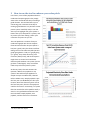
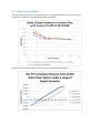
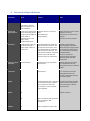
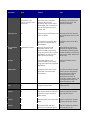
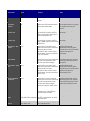
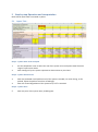
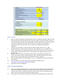
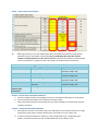
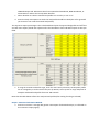
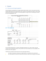
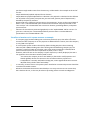
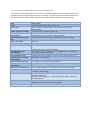
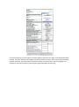
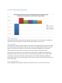
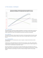
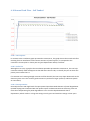
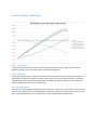
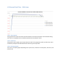
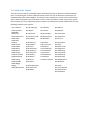
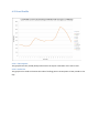
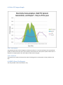
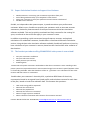
SunWiz PV Sales Tool User Manual
Calculating and Communicating PV’s Financial Outcomes to Staff and Customers
Prepared by: Warwick Johnston
Document Revision: 0
Software Revision: 1.4b
1
Innovation, Expertise, Independence
1
Introduction
The SunWiz PV Sales Tool is intended to assist in the evaluation of the financial outcome resulting
from installation of a solar power system. It contains many graphs, tables, and charts that can assist
in conveying a sales message. It is intended for in-house use in solar power companies, but can easily
be extended, in recognition that most users of the tool wish to customize their own sales message.
There are restrictions placed upon fields that can be manipulated. This is done in order to protect the
novice user from inadvertently changing a cell containing an automatically-updating formula upon
which calculations depend. Cells that are user-modifiable are highlighted in yellow. Expert users
wishing to customize the spreadsheet may request a password that unlocks all cells. Alternatively, an
automatically-updating spreadsheet can be added that references cells within the supplied
workbook.
This user guide accompanies the MS Excel workbook. It consists of three parts:
1. An introduction to the features of the workbook, and an overview of the spreadsheets.
2. A step-by-step guide for beginners to operate the workbook.
3. Description of the major outputs from the spreadsheet, and their value in a sales pitch.
In addition, guidance is contained in comments within the spreadsheet, and in the “how to use” tab
at the start of the workbook.
Some familiarity with MS Excel is assumed. For those less-familiar with the operation of MS Excel, a
bar exists at the bottom of the Excel program (see image below) that allows users to switch between
spreadsheets (also referred to as “tabs”) in the workbook. As more tabs exist than can be displayed
on screen at once, use the arrows on the left (< and >) to scroll the tabs left and right. To change tab,
simply click on the desired spreadsheet name across the bottom of the page.
Use the horizontal and vertical scroll bars to move around a single spreadsheet, and use the zoom to
enlarge the numbers on screen (see image below)
2
Workbook Features
The SunWiz PV Sales Tool is designed to simplify the process of financial evaluation of a PV system
under a range of circumstances. It contains many complex formulae to calculate revenue, payback,
internal rate of return (“effective interest rate”), and cash flow. This ensures that solar businesses can
spend their time selling and installing, backed by a tool that accurately performs the calculations
they need to convince customers to purchase from them.
The SunWiz PV Sales Tool contains:
·
·
User-controllable:
- solar power system performance inputs,
- state of Australia,
- REC (renewable energy certificate) price,
- REC multiplier,
- REC zone,
- year of analysis,
- grid electricity price and annual increase,
- annual panel degradation, and
- premium price above Feed-in Tariff (FiT, also known as a “solar bonus scheme” in
some states).
Automatically calculated:
- number of RECs,
- net or gross FiT, and
- remaining duration of Feed-in Tariff.
- Comparison of 6 solar power systems, with user-controllable solar power system
prices.
- Automatically calculated post-REC system customer prices.
- Automatically calculated annual revenue and simple payback.
- User-controllable range of (net FiT) export power percentage to help solar
businesses understand the sensitivity of payback to export.
The SunWiz PV Sales Tool provides these handy sales tools:
-
-
-
Calculation of the likely amount of solar power export by each of the selected
systems, and the consequent payback, displayed as a table and in chart form.
Quantifiable demonstration that larger solar power systems typically have
quicker payback, and demonstration of the benefit of saving daytime
electricity consumption.
Detailed financial investigation of one of the six chosen solar power system
sizes, including post GST price, post-tax cost, 20 year depreciation calculation,
simple payback, and internal rate of return.
Charts of customer price net of solar credits, payback and IRR vs. export
power percentage.
Cash flow calculation and charts for various electricity consumption levels
with and without loans.
A customer summary sheet, useful for printing
3 How to use the tool to enhance your sales pitch.
Let’s face it; most of the population doesn’t
understand complex graphs. They simply
want to be reassured that they’re making a
good decision. This tool will assist you in
convincing your customers that they’re
making a good decision 1 to purchase a solar
power system. Carefully used, it can also
assist you to highlight why your system is
better than your competitors’ systems, and
to protect you from making a claim your
customer may later sue you for.
This tool produces a number of easy to
understand graphs. Bar charts compare
financial outcome after 20 years (No PV =
bad, PV = good). They also show cash flow
taking into account electricity bills (No PV =
graph going down = bad; PV = graph going
up = good). They show electricity price
increases (always bad), and what impact it
might have on annual and cumulative
electricity bills without a PV system (curves
go down  bad again). They can also be
used to up-sell a solar power system.
At the very least, this tool answers the
question “What is the payback on my
system?” But while simple payback is a
simple concept to understand, it doesn’t
tell the whole story. Simple payback is just
the first year cost divided by the first year
revenue. But if the electricity price rises in
the first few years, then the true payback
could be far sooner. Conversely, if a system
fails the month after it has paid for itself, it
wasn’t a very profitable investment. This
tool calculates simple payback, true
payback, and the return on investment.
1
Or not, as the case may be
The return on investment is expressed in terms of Internal Rate of Return (IRR). While this can be
complex to understand and convey, put simply it’s the “effective interest rate on your investment”.
If the IRR is greater than the interest rate a bank will give you on a bond, then it could be considered
a sensible financial investment (depending on the risk involved in the investment).
Solar power could be considered a risky investment in states with net Feed-in Tariffs, as the revenue
can vary by a factor of three depending on a site’s daytime power consumption. Fortunately, this
tool substantially reduces this risk by calculating the likely amount of generated power that is
export, and thus the corresponding likely revenue, likely simple payback, likely true payback, and
likely IRR. Of course, a model is only as good as its assumptions and inputs, so use this tool wisely.
3.1 Export Calculation
For those selling in states with net Feed-in Tariffs, a correct calculation of the amount of power that
is exported is essential to your payback calculations. Exports can be calculated in one of three ways,
as illustrated below. The ‘Measured’ method is the simplest and most accurate to use, if you have a
residential customer with daily power consumption between 12 and 21 kWh/day. If not, you can
enter an hourly load profile for each month of the year, from which a synthesized load is created for
each hour of the year, and compared to predicted solar generation in your selected nearest capital
city (other locations available too). Otherwise, use Custom to provide your best estimate, and a
sensible range.
Custom
Load Profile
•Enter Your Own Assumed
Export %
•Show a Range of Possible
Outcomes
•Enter Estimated Load Profile
•Scale to household's daily
consumption if necessary
•Select your Location (Solar
Output Data Loads)
•Calculation based upon
hourly calculation of load
profile and solar radiation
Measured (Residential
Only)
•Based on UNSW
Measurements of 30
Newington Residences with
PV systems, projected to
larger residential systems
•Calculates Likely Export for 3
levels of daily power
consumption
3.2 Multi-System Analysis
The tool allows you to enter six system sizes, prices, and performances. All six are shown for
comparison purposes for the Measured Export Calculation.
Otherwise all the graphs reflect the chosen system size for deeper analysis.
4 Overview of Spread sheets.
Spreadsheet
Inputs
Outputs
Value
Inputs
Government support and
performance-relevant
inputs that apply to the
whole workbook.
Export Percentages.
Revenue and
simple payback
A range of six system sizes
and corresponding prices.
A range of percentages of
export power to
investigate under a net
Feed-in Tariff.
A range of REC prices.
Customer Price pre- and postRECs.
Annual Revenue.
Simple Payback.
Quick assessment of the impact
of system price and
performance on revenue and
payback.
REC price sensitivity analysis.
Tax Analysis
A single system size to be
financially analysed in
greater depth. Refers to
“Inputs” tab.
Price breakdown for residential
and commercial customers. Pretax and post-tax revenue, more
accurate payback for residential
and commercial customers, and
Internal Rate of Return (“effective
interest rate”) that takes into
account rising cost of electricity.
Provide customers with a
tailored payback calculation.
Demonstrate the large discount
on commercial systems due to
the combination of GST, RECs,
and depreciation.
Convince commercial
customers with investment
decisions based upon IRR
hurdle rates.
Customer Output - Customer Details
Residential
Linked summary of data within
spread sheet.
Displays snapshot of analysis
for a residential customer,
along with summary of relevant
graphs.
Customer Output
Commercial
Customer Details
Linked summary of data within
spread sheet.
Displays snapshot of analysis
for a commercial customer
(taking Depreciation into
account), along with summary
of relevant graphs.
Likely Net FiT
payback
As specified in “Inputs”
tab.
For net FiTs, the likely amount of
generated power that is exported
for the selected range of system
sizes, based upon electricity
consumption, and consequent
simple payback.
Provide customers with a moreaccurate and realistic estimate
of their revenue and payback
that is based upon industry
measurements.
Likely Gross FiT
payback
As specified in “Inputs”
tab.
Simple payback for gross FiTs.
A quick analysis of simple
payback under FiT.
DCF Analysis
As specified in “Inputs”
tab.
Discounted cash flow over 20
years. The details that lay behind
the “Tax Analysis” IRR
calculations.
Depreciation
Schedule.
As specified in “Inputs”
tab.
Depreciation analysis for system
that is selected on “Inputs” tab.
Spreadsheet
Inputs
Outputs
Value
Cashflow
Annual electricity
consumption, loan
amount, loan term, and
interest rate.
Annual and cumulative flow of
cash based upon customer’s
electricity bill and solar
generation with various export
percentages, with and without a
loan, for the system chosen in
“Inputs” tab.
Demonstrate the insulation
provided by a PV system from
rising electricity prices, and
possible profitability.
Projected
Electricity Price
As specified in “Inputs”
tab.
Graphs the increasing costs of
Shows the expected rise in
electricity against the steady costs electricity prices over 20 years,
of the PV system.
against the steady price of a PV
system.
Price Breakdown
As specified in “Inputs”
tab.
Graph of the effective price paid
by commercial customers after
GST, RECs, and depreciation is
accounted for.
Visually convince commercial
customers of the savings they
receive.
Net FiT Payback
and IRR
As specified in “Inputs”
tab.
Graph of commercial and
residential payback, and
commercial IRR incorporating
rising cost of electricity and panel
degradation, as they vary with
export power percentage.
Demonstrate to commercial
customers that good benefits
are available, and even greater
benefits are within reach if they
export more power. Relevant to
Net FiT only.
Gross FiT payback
IRR Chart
As specified in “Inputs”
tab.
Bar chart of commercial and
Demonstrate the favourable
residential payback, and
outcomes available under a
commercial IRR incorporating
gross FiT.
rising cost of electricity and panel
degradation.
Likely Net FiT
Payback Chart
As specified in “Inputs”
tab.
Graph of the likely payback from
a range of system sizes, under
three levels of annual power
consumption.
Provide customers with a moreaccurate and realistic estimate
of their revenue and payback
that is based upon industry
measurements. Visually
demonstrate the value of
investing in a larger system, and
of saving daytime energy use.
Relevant to Net FiT only.
Gross Fit Payback
Chart
As specified in “Inputs”
tab.
Graph of the likely payback from
a range of system sizes.
Visually demonstrate paybacks
under Gross FiT.
Net Fit Solar
Revenue
As specified in “Inputs”
tab.
Graph showing annual revenue
over 20y period for the selected
system size, using a variety of
export values.
Shows how much revenue a
system can produce annually
over a 20 year period.
Gross FiT Solar
Revenue
As specified in “Inputs”
tab.
Graph showing Revenue on the
Shows maximum amount of
selected system size if export was revenue a system can produce
100%
annually over 20 year period.
Net FiT Cumulative As specified in “Inputs”
Revenue
tab.
Graph showing revenue
accumulated over a 20 year
period, for the selected system
Shows how much accumulated
revenue a system can produce
over a 20 year period.
Spreadsheet
Inputs
Outputs
Value
size, using a variety of export
values.
Gross FiT
cumulative
Revenue
As specified in “Inputs”
tab.
Graph showing accumulated
Revenue on the selected system
size if export was 100%.
Shows maximum amount of
accumulated revenue a system
can produce over 20 year
period.
Net Financial
position nFit
Bar Graph of possible Saving
incurred over a 20 year period,
with varying export amounts on
the chosen system size.
Demonstrates savings on
electricity.
Net Financial
position qFiT
Bar Graph of possible Saving
Demonstrates savings on
incurred over a 20 year period,
electricity.
with a 100% export on the chosen
system size.
Net Position - Self
funded
none
Graph of the cumulative cash
flow cash based upon customer’s
electricity bill and solar
generation with various export
percentages, assuming customer
pays cost upfront.
Visually demonstrate
cumulative electricity spent
over 20 years, and comparative
profit if a PV system is
purchased.
Annual Cash Flow
- self funded
None
Graph of the annual cash flow
based upon customer’s electricity
bill and solar generation with
various export percentages.
Visually demonstrate annual
electricity spent over 20 years,
and comparative profit with a
PV system.
Net position - with None
loan
Graph of the cumulative cash
flow cash based upon customer’s
electricity bill and solar
generation with various export
percentages, assuming customer
takes a loan.
Visually demonstrate
cumulative electricity spent
over 20 years, and comparative
profit if a PV system is
purchased via loan.
Annual Cash Flow
– with loan
None
Graph of the annual cash flow
based upon customer’s electricity
bill and solar generation with
various export percentages,
assuming customer takes a loan.
Visually demonstrate annual
electricity spent over 20 years,
and comparative profit if a PV
system is purchased via loan.
1kW solar Output
Location, load Profile.
Calculates hourly energy
generation for a 1kW system,
includes state variables.
Hourly system performance.
Net FiT output
graph
Day of year, generated
Energy consumption and export
from 1kW solar output tab. using a 1.5 kW system, for each
day of the year.
RECs Zone, Fits,
Exports.
Location, load profile for
each system size.
Daily system performance.
Cash outcomes comparing system REC's received over the year.
sizes and REC zones.
5
Step-by-step Operation and Interpretation
Note that all input fields are marked in yellow
5.1 Inputs Tab –
Step 1 – System Sizes to be Analysed
1.
2.
Use the drop-down arrow to select the size of the system to be analysed in detail from the
range of system sizes below.
Enter a Range of up to 6 system capacities to demonstrate to your client.
Step 2 – System Performance
3.
4.
Enter the predicted actual performance (If the system is shaded, non-north facing, or flat
pitched, adjust the performance here accordingly).
Enter the annual degradation of the system here, 0.5% is standard.
Step 3 – System Price
5.
Enter the price of the system here, excluding GST.
Step 4 - Location
6.
7.
8.
9.
10.
11.
Enter the state of installation and Location (SA, ACT, VIC, NSW, QLD, TAS, NT or WA). This will
automatically select the feed-in tariff rate, type (net or gross), and the remaining number of
years of premium FiT. Graph titles automatically update to indicate whether they are relevant
to the type of applicable FiT. Select “NA” for sites not receiving a FiT, for example, a
commercial site or sites with system size or electricity consumption exceeding FiT
regulations.
To apply a 1-for-1 Retail FiT, select NA and set ‘When Fit Ends, Earn 1-for-1’ to TRUE.
Enter the behaviour at the conclusion of the FiT, select TRUE for 1-for-1 or FALSE for PV
specific. After the FiT ends, exported power may attract a PV specific value or the same rate
as the retail consumption tariff (1-for-1). Select TRUE for ACT, TAS and NT and Vic SFiT to
provide 1-for-1.
Enter the year of analysis. The remaining FiT duration is automatically calculated. WA
remains at 10 years duration, regardless of start date, until being reduced in 2021 (after
which the price of electricity is likely to be higher than the FiT anyway).
Enter the REC multiplier, which should be 5, 4, 3, 2, or 1, depending on the year and month
of installation.
Enter the REC Zone, which is based on the postcode of installation (see
http://www.orer.gov.au/sgu/index.html for details).
Type the STC price, excluding GST.
Step 5 – Commercial Parameters
12.
13.
Enter your tax bracket and GST % here. If the system is to be sold to a commercial customer,
enter the tax bracket of the business to which it’s sold. Most commonly this is 30%. If the
system is to be sold to a residential customer, enter 0% in this cell. This cell influences the
post-tax cost and revenue (including value of depreciation).
If the system is to be sold to a commercial customer that is registered for GST, enter “10%”.
14.
15.
Otherwise enter 0%. This cell influences the post-tax cost and revenue.
Enter the depreciation rate. 10% is the standard rate, which uses the current ATO 20-year
product lifetime. Small businesses may be able to use a 30% depreciation rate.
Enter the discount rate you wish to use to calculate the net present value (NPV) in the
discounted cash flow analysis.
Step 6 – Electricity Prices
16.
17.
18.
19.
20.
Enter the compounding growth in electricity price from year to year
Enter the fixed electricity import price $0.18/kWh (incl GST). This should be the ‘average’
price paid by the customer, as reflected on their bills. Time-of-use tariffs are not supported in
this version of the tool. More specifically, this should be the average price earned by the PV
system taking into account time of generation.
Enter the price expected for solar earnings when the FiT ends (note that no adder will be
added). If 1-for-1 is TRUE (location section), these values are ignored
Enter the LGC price for each year, which applies if ‘Deem RECs’ is set to FALSE, otherwise
enter the STC price.
Adder to Regular FiT - If the customer receives a premium rate above the state-mandated FiT
(some electricity retailers such as Origin provide an additional $0.06/kWh), enter it here.
Note that at the end of the FiT, this adder does not apply.
Step 7 – Additional costs
21.
22.
Enter any additional yearly PV related costs including GST here, e.g. maintenance costs or
extra equipment needed. This affects the PV revenue, cash flow, and true payback
calculations.
Enter any extra yearly bill related costs here (such as service charges un-related to electricity
consumption levels), including GST. This affects the cash flow and net financial position
graphs for both ‘non PV’ and PV solution. It doesn’t affect the PV revenue graphs.
Step 8 - Cashflow Factors
If the customer is purchasing the system on finance, enter the details here.
23.
24.
25.
Enter Loan amount. (Deposit amount is automatically calculated as purchase price less loan
amount). Hint: Set “=C51” to automatically adjust to the full system price
Enter loan term.
Enter interest rate of loan.
The effective Post Tax annual Payment is calculated
Step 9 – Power Export Search Space
26.
Referring to Section 3.1 or the table below, select the preferred method of export power
methods (custom, load profile, measured). The corresponding data from the relevant
column is transferred across to the “Used” column. Utilise the check boxes to automatically
remove unused lines in graphs and the unused parts of the DCF analysis worksheet.
Client
Suggestions for Export Calculation Method
Power Usage
Export Calculation Method
Residential
In range 9-23 kWh/day
Residential
Outside range 9-23 kWh/day
Commercial
Feed-in Tariff eligible
Commercial
Feed-in tariff ineligible - select
state=NA
For a range of possible outcomes
Quick analysis
(commercial/
residential)
Use measured – refer to
'customer output' tab.
Use load profile - refer to
'customer output tab.
Use load profile - refer to
'customer output' tab.
Use load profile - refer to
'customer output' tab.
Use custom.
Step 9a – Custom Export Calculation Method
a. Enter the range of export percentages you wish to investigate and display on some graphs
b. Enter the Daily Consumption (for cash flow calculations only)
c. Select the nominated export percentage that you wish to display on the bar charts and the
customer summary
Step 9b – Load Profile Calculation Method
a. Enter Nearest Location. This loads hourly solar radiation for that location based on a 1 kWp
north-facing solar power system inclined at 30°, and scales it to your system size
b. If you have hourly-load data for a full year, select Load Profile Type = ‘8760-hour load
profile’, and paste the data into the ‘Custom 8760-Hour Load’ column in the
1kWSolarOutput tab. Otherwise select from Queensland Residential, NSW Residential, or
select Manual and use the hourly tables beneath.
c. Select whether to scale the manual load profile to a set value, or use ‘as is’.
d. Enter the daily consumption to which the load profile should be scaled (this cell is ignored if
you choose to not scale the manual load profile).
The customer export percentage is thus calculated based upon the entered load profile and 10% less
and 10% more export placed into adjacent cells. The boundaries of 0% and 100% export are also prefilled.
e. If using the manual Load Profile Type, enter the site’s hourly electricity consumption profile
for an average day in each month of the year (in Watts). You may wish to copy and paste an
example residential load profile from row 100 onwards
Note that the table below reflects the analyses load profile (after scaling if scaling is selected).
Step 9c – Measured Calculation Method
a. Enter the customer’s average daily power consumption for detailed analysis, as reflected on
the customer output page(s).
Step 10 – Time of Use Calculator
a. Enter electricity prices for peak, shoulder and off-peak periods, setting the appropriate
periods in the area beneath. Then press the “Use Value in Calcs” button on row 138. This
will copy an average value for the electricity price into cell B55 above. The average is
weighted by the load profile. If you do not want to use the calculator but use your own
average electricity price figure instead, then enter it directly into cell B55.
b. Enter values for TOU demand charges if appropriate. If demand charges are flat rate then
leave the shoulder and off-peak cells empty. “Enable demand reduction” (cell D86) must be
set to true for this to be taken into account. Note that using the default load profiles gives
residential consumption patterns (e.g. and evening peak) so no demand reduction value will
be generated. To give a realistic estimate of the value, the estimated demand profile, with
reduced peak consumption, should be entered in the Manual Load Profile cells.
6 Outputs
6.1 Revenue and simple payback
This tab facilitates investigation of a range of power exports under a net FiT. First-year revenue and
simple payback (upfront cost divided by first-year revenue) is presented numerically for the selected
range of power export percentages. If the simple payback is longer than the remaining FiT duration,
the cells are highlighted in red.
6.2 Tax Analysis
The tax analysis tab presents a summary of detailed calculations on a chosen system, for both
commercial and residential customers. This provides users with the ability to convey payback, and
internal rate of return figures.
Calculations are made from data entered on the input page and show The effect of GST, RECs, and 20 years of depreciation on the effective net system price
Pre-tax and post-tax revenue for commercial customers. Note the tax savings on the upfront
purchases imply taxed income from the PV array, as illustrated in the example at the end of
this list.
Simple Residential payback adjusted for FiT duration
Simple Business payback adjusted for FiT duration. The payback is calculated as the effective
out-of-pocket cost (system price post GST, post tax break, post 20 years of depreciation)
divided by the post-tax revenue.
Business IRR is the “effective interest rate on the investment”, known as the Internal Rate of
Return. This is calculated based upon the discounted cash flow analysis presented on the
“DCF analysis” tab. The IRR takes into account FiT duration, panel degradation, and power
price increases.
Elements of this table are presented graphically on the “Payback&IRR” tab for net FiTs. If a
gross FiT is selected, the “GrossFiTPaybackChart presents these. Price breakdown is
presented on the “PriceBreakdown” tab.
The effect of taxation on PV system revenue: an example
If a company pays $1100 including GST in electricity bills each year, then after 10% GST is
claimed and 30% company tax on the payment is deducted from revenue, then the company
is only $700 out of pocket.
If a solar power system reduces their bill by $220 including GST, then their remaining
electricity bill is $880 including GST. After claiming GST and deducting company tax, the
company is now only $560 out of pocket. Their solar power system thus created $140 in
post-tax revenue (note that this is equivalent to $220 / 110 % * 70%).
However, while the GST on the company’s import electricity is clearly displayed, the GST is
not applied to the Solar Bonus Scheme/Feed-in Tariff.
- This means the company incurs a GST liability on the Feed-in Tariff payments and
should rightfully declare this income to the tax office and thus pay GST on it.
- A 44c/kWh FiT is actually 44c/kWh including GST; a GST-registered business receives
40c/kWh if they declare their GST liability ².
In summary, revenue from a solar power system installed on commercial premises should be
considered as taxable income.
Whether the business declares this GST liability or not is up to them. Do not assume they
don’t declare this tax, as this may be taken as providing advice to evade tax obligations
6.3 Customer Output Residential/Commercial
The Customer Output Tab presents a summary of the data contained within the spread sheet. This is
useful for printing a tailored assessment for a customer. The only inputs that should be adjusted on
this sheet are the customer details. The remaining cells should be adjusted on the Inputs Tab.
Field
State
System Size
System Price RRP incl GST
Discounted System Price
incl/excl GST
Discounted $/W incl/excl
GST
Feed in Tariff Type
Feed in Tariff Rate
Analysis based on
Average daily power
consumption
Estimated Generation
Approximate % of Power
Consumption:
Estimated Export Per Year:
(As a percentage of
Generation):
Estimated Annual Revenue:
Simple ROI
Estimated Simple Payback:
Calculated True Payback:
Internal Rate of Return
Value/ Notes.
QLD, VIC, NSW, ACT, SA, WA, NT, TAS, NA
Values and graphs below apply to the selected system size, as
displayed here
Pre -REC price for selected system size.
Post-REC price for selected system size. Note that GST reductions are
applied if GST is not set to 0% on the inputs page.
Post-REC post GST (if selected) price divided by system capacity
Net/Gross
Standard + Premium FiT
Estimated Load Profile / Residential Measurements / Estimated Export
%,
(reflective of chosen export % method)
Daily consumption as selected on inputs page and as corresponding
with export calculation method
System performance entered on inputs tab for selected system size
Generation ÷ Consumption
As calculated from Generation and Export %
Export % output from chosen export calculation method
First-year Revenue (pre-tax, and post-tax on the commercial tab)
Return on investment based on upfront cost and first year revenue
(i.e. with no discounting)
First year discounted price ÷ First year Revenue.
Commercial Tab uses:
(First year discounted price – twenty-years depreciation) ÷ Post Tax
First year Revenue
True payback accounting for rising electricity prices, panel
degradation, and depreciation (if tax applies).
Effective Interest Rate on Investment (over 20 years).
You are welcome to put your logo and contact details at the top of the page. Some checkboxes with
‘leading’ customer advice are provided at the bottom of the summary, which can be printed and left
with the customer. The remainder of these charts show a summary of the important graphs. It is
possible to print these neatly by selecting each graph individually and printing.
6.4 Likely Net FiT Payback
This graph provides industry-measured PV generation in relation to three categories of daily
residential electricity consumption, and the corresponding export from a 1-3kW PV system.
Naturally, the time of day of consumption will influence a particular customer’s outcome, but this
data provides a baseline estimate calculated from measurements rather than pure guesses. This
data is most accurate for Sydney solar radiation and energy consumption.
The second graph shows the same data, projected to larger system sizes, with data points at each of
the system sizes selected in the “Inputs” tab.
This data is only relevant for residential systems, and ignores the likelihood that a house with a roof
large enough to hold a 10kW system would have very high power consumption.
The value of the graphs lies is in demonstrating the large increase in exported power from a small
increase in system size, or from a decrease in power consumption. This is translated into simple
payback (highlighted red where the simple payback exceeds the remaining FiT duration), and
illustrated graphically in the ‘LikelyNetFitPaybackChart’ tab.
Note that some chart titles will automatically update, and remind you that they are irrelevant if a
gross FiT is selected.
6.5 Likely Gross FiT Payback
This tab shows the same information as the Likely Net FiT Payback tab, except for a gross FiT (with
100% of the energy generation being exported). Note that some chart titles will automatically
update, and remind you that they are irrelevant if a net FiT is selected.
6.6 DCF Analysis (Discounted Cash Flow)
This tab shows the workings of the true payback and IRR calculations. It calculates the true payback
of a system, taking into account increasing prices of electricity, panel degradation, post tax revenue
and PV-related expenses, and depreciation of the system, over a user defined period (default 25
years). The analysis is repeated for each of the export % in the range selected on the inputs tab.
Note that the PV-Related additional costs affect this analysis; the Bill-related additional costs do not.
6.7 Depreciation Schedule
This tab calculates the depreciation of the system over a 20 year period using the Australian Tax
Office mandated depreciation value of 10% pa.
6.8 Cash Flow
The “Cashflow” tab provides operators the opportunity to demonstrate the effect of rising power
prices on customer’s annual and 25-year electricity spend.
The electricity bill, solar revenue, and depreciation are calculated for each of 20 years, accounting for
panel degradation and the increase in the price of imported electricity. Any PV-related cost is
reflected in the electricity revenue, and any bill-related costs are reflected in the Electricity cost.
Accumulated cash flow is presented in the ‘net position – self funded’ table, assuming the full cost of
the system is paid up front. This cash flow is presented graphically in the “Net Position – Self
Funded” tab.
Annual cash flow is presented in the ‘annual cash flow – with loan’ table, with details of the loan.
This cash flow is presented graphically in the “Annual Cashflow – self funded” tab.
Accumulated cash flow is presented in the ‘net position – with loan’ table, with details of the loan.
This cash flow is presented graphically in the “Net Position – with loan” tab.
Annual cash flow is presented in the ‘annual cash flow – with loan’ table, with details of the loan.
This cash flow is presented graphically in the “Annual Cashflow, with loan” tab.
6.9 Projected Electricity Price
6.9.1 Description
This graph shows the electricity price that will occur if the assumptions about annual compound
growth entered in the inputs hold true.
6.9.2 Sales Use
This could be used to suggest to customers how soon a doubling in electricity price could occur. This
may encourage customers to purchase a system that provides them with a fixed-cost electricity
source: solar power.
6.9.3 Interpretation
The red line displays the annual compound electricity price growth entered in the inputs page. The
blue line shows the resulting average electricity price paid.
6.10 Net FiT Payback and IRR
6.10.1 Description
This graph shows the simple payback, true payback, and Internal Rate of Return for the nominated
system over the used range of export power percentages.
6.10.2 Sales Use
Show customers their likely true payback and internal rate of return, and what might happen if they
reduce their power consumption by a little. Provide confidence that the worst-case outcome (no
export) isn’t really so bad after all, so they’re almost certainly going to have a good outcome
regardless of the amount of power they export. Show customers how honest and truthful your
calculations are.
6.10.3 Interpretation
Read payback (green and purple lines) off the left axis. Read IRR (blue line) off the right axis. Each of
the used export power percentages has a marker.
The True payback is often less than the simple payback for low export percentages on a net FiT. This
is because financial outcome on systems with low exports is more affected by rising electricity prices
than systems earning mostly FiT (which remains constant each year). The simple payback can by
shorter than the true payback as it doesn’t account for depreciation or degradation.
6.11 Likely Net FiT Payback Chart
6.11.1 Description
This graph shows the likely simple payback for the chosen range of system sizes using the measured
export calculation method.
6.11.2 Sales Use
This chart can be very effective in conveying a sales message that encourages up-sizing and crossselling of energy efficiency products. Looking vertically at this chart (fixed system size, variable
power consumption) demonstrates to the customer the value of energy efficiency, which can result
in much quicker payback. Looking horizontally at this chart (fixed power consumption, variable
system size) may demonstrate to the customer the value of increasing system size, which will result
to significantly more export power and revenue and might result in quicker payback, depending on
your system and REC prices. Remember however, that payback is just one way of evaluating a solar
outcome. For example, if a replacement inverter is required during the life of the panels, a larger
inverter costs proportionally less than a smaller inverter, thus having a smaller impact upon the
overall financial profitability.
6.11.3 Interpretation
This graph shows the likely simple payback of 6 systems, by evaluating the likely amount of power
exported from each system (based on industry measurement and calculations presented in the
“Likely net-FiT Payback” tab), the likely amount of revenue can be calculated, and thus the likely
payback.
6.12 Gross FiT Payback Chart
6.12.1 Description
This graph shows the likely simple payback for the chosen range of system sizes on a gross FiT. This is
the gross FiT equivalent graph to that shown in Section 6.13.
6.12.2 Sales Use
This chart (fixed power consumption, variable system size) may demonstrate to the customer the
value of increasing system size, depending on your system and REC prices. Remember however, that
payback is just one way of evaluating a solar outcome. For example, if a replacement inverter is
required during the life of the panels, a larger inverter costs proportionally less than a smaller
inverter, thus having a smaller impact upon the overall financial profitability
6.12.3 Interpretation
This graph shows the simple payback of 6 systems
6.13 Net FiT Solar Revenue
6.13.1 Description
This graph shows the post-tax annual revenue from electricity sales of the selected solar power
system, for the selected range of export percentages on a net FiT.
6.13.2 Sales Use
This graph can be used to visually demonstrate how the amount of revenue created the solar power
system may effectively increase over time (especially for low export percentages), as the electricity
price increases.
6.13.3 Interpretation
The competing effect of panel degradation and increasing electricity prices can be seen in this graph.
Revenue under 100% export declines with degradation until (under the assumptions of a 7% annual
increase in electricity price), export power has the same value of the import power. At this stage, the
electricity price growth is greater than panel degradation, so the curve trends upwards. Western
Australian customers might also see the end of the FiT displayed clearly on their graph.
6.14 Net FiT Cumulative Revenue
6.14.1 Description
This graph shows the cumulative post-tax position of a customer that has bought the selected solar
power system, for the selected range of export percentages on a net FiT.
6.14.2 Sales Use
This graph can be used to demonstrate the customer’s initial outlay is more than paid back within
the life of the system, that they can earn two to three times their investment.
6.14.3 Interpretation
True payback occurs when the relevant line crosses the x-axis.
6.15 Net Financial position nFiT
6.15.1 Description
This graph shows the cumulative post-tax position 20 years after a customer that has bought the
selected solar power system, for a range of export percentages under a net FiT.
6.15.2 Sales Use
This graph can be used to simply compare the customer’s net financial position if they don’t install
PV, or their likely financial position if they do, with a best case (100% export) and worst case (0%
export). It can show the customer the scary amount of electricity expenditure over 20 years,
compared with an initial outlay of a smaller amount that results in a far greater profit.
Note that for a small system size, PV installation may still result in a negative financial position
(although still better than no purchase). This is because power production is far less than power
consumption, and thus the customer’s electricity bill isn’t fully offset (especially considering
increased electricity prices). Thus this graph can be used to up-sell to a system that covers more of
their energy usage.
6.15.3 Interpretation
Pretty straightforward: Would you rather be on the left-most bar, or one of the other bars?
6.16 Net Financial Position qFiT
6.16.1 Description
This graph shows the cumulative post-tax position 20 years after a customer that has bought the
selected solar power system, for a gross FiT.
6.16.2 Sales Use
This graph can be used to simply compare the customer’s net financial position if they don’t install
PV, or their likely financial position if they do, with a best case (100% export) and worst case (0%
export). It can show the customer the scary amount of electricity expenditure over 20 years,
compared with an initial outlay of a smaller amount that results in a far greater profit.
Note that for a small system size, PV installation may still result in a negative financial position
(although still better than no purchase). This is because power production is far less than power
consumption, and thus the customer’s electricity bill isn’t fully offset (especially considering
increased electricity prices). Thus this graph can be used to up-sell to a system that covers more of
their energy usage.
6.16.3 Interpretation
Pretty straightforward: Would you rather be on the left-most bar, or the right-most bar?
6.17 Net Position – Self Funded
6.17.1 Description
This graph show the customers cumulative expenditure on electricity and solar power, taking into
account any additional PV-related and bill-related costs. This is similar to the PV revenue graph
shown in Sections 6.15 and 6.16, but includes money spent on electricity consumption.
6.17.2 Sales Use
This graph can be used to simply compare the customer’s net financial position if they don’t install
PV, or their likely financial position if they do, with a best case (100% export) and worst case (0%
export).
6.17.3 Interpretation
This graph presents a cumulative position, which is simpler to interpret than annual cash flow
presented later.
Simplistically, the downwards going curve shows that not investing in a PV is bad, especially when
compared with the upwards curve that results from a PV purchase. Payback is where the green line
crosses the line associated with the expected PV export.
Note that installation of a small system at a location with high power consumption may result in a
graph in which all lines trend downwards. Similar may occur in NSW after the end of the FiT. Though
still better off than not purchasing a PV system, this may encourage customers to buy a larger
system.
6.18 Annual Cash Flow – Self Funded
6.18.1 Description
In contrast to the cumulative graph presented in Section 6.21, this graph shows the annual cash flow
resulting from PV installation under various amounts of power exports, as compared to the
customer’s electricity bill. It shows post tax (post depreciation offset) cash flow.
6.18.2 Sales Use
Although not as scary a graph as the cumulative equivalent presented in Section 6.21, this can help
customers identify what will happen to their bill when the FiT ends, or identify the year in which the
power price reaches the FiT.
If a customer isn’t creating enough revenue to offset their bill, the lines may slope downwards as the
electricity price rises. This can be a good incentive to purchase a larger system (or add more panels
at a later date).
6.18.3 Interpretation
Generally the lines with high levels of export power slope downwards because of panel degradation.
Upward sloping lines associated with low power export can demonstrate that electricity prices are
more than compensating for panel degradation. Lines can also slope downwards due to
depreciation, which results in a large tax savings in early years and small tax savings in later years.
6.19 Net Position – With Loan
6.19.1 Description
This graph shows net financial position if the customer takes out a loan to pay for their system.
Similarly to Section 6.21, this graph shows cumulative expenditure.
6.19.2 Sales Use
This graph may illustrate to customers that if they refinance their home loan, their net position is not
much worse off while they repay the system, after which they are far ahead. Effectively, instead of
paying a larger electricity bill, the savings from their electricity bill pay off their system. After their
system is paid off, they can have free electricity.
6.19.3 Interpretation
This can be a complex graph, depending on the system size, customer’s consumption, loan term, and
interest rate. When the line associated with the customer’s purchase sits above the green line, then
they’re ahead (paid back). In the example above, they’re ahead from the beginning.
6.20 Annual Cash Flow – With Loan
6.20.1 Description
This graph shows annual cash flow associated with the net financial position associated with taking
out a loan, as compared to the cumulative position that was shown in 6.23.
6.20.2 Sales Use
This graph is quite complex, but clearly shows the end of the repayment period, and the many years
of electricity cheques that follow before the electricity price skyrockets.
6.20.3 Interpretation
This can be a complex graph, depending on the system size, customer’s consumption, loan term, and
interest rate.
6.21 1kW Solar Output
This tab is mostly used for load profile export calculation purposes. It shows the simulated output
from a north-facing 30°-inclined 1 kW solar power system for each of Australia’s capital cities (as
simulated using Solar Advisor Model). This output is then scaled by the system size to calculate the
export, when compared to the load. There is also a column that allows custom solar power system
to be entered (e.g. from a different location). SunWiz can provide hourly solar radiation data for the
following locations upon request.
ACT-Canberra
NSW-Armidale
NSW-Blue
Mountains
NSW-Cabramurra
NSW-Cobar
NSW-Coffs
Harbour
NSW-Cooma
NSW-Dubbo
NSW-Moree
NSW-Nowra
NSW-Orange
NSW-Parramatta
NSW-Richmond
NSW-Sydney
NSW-Thredbo
NSW-Wagga
Wagga
NSW-Williamtown
NT-Alice Springs
NT-Darwin
SA-Adelaide
SA-Ceduna
WA-Albany
WA-Broome
NT-Katherine
NT-Tennant Creek
QLD-Amberly
SA-Mt Gambier
SA-Roxby Downs
SA-Woomera
WA-Carnarvon
WA-Esperance
WA-Forrest
QLD-Atherton
QLD-Brisbane
QLD-Cairns
QLD-Charleville
QLD-Gladstone
QLD-Longreach
QLD-Mackay
QLD-Maleny
QLD-Mt Isa
QLD-Oakey
TAS-Hobart
TAS-Launceston
VIC-Ballarat
VIC-Cape Otway
VIC-Coldstream
VIC-East Sale
VIC-Melbourne
VIC-Mildura
VIC-Warrnambool
WA-Geraldton
WA-Giles
WA-Halls Creek
WA-Kalgoorlie
WA-Katanning
WA-Learmonth
WA-Mandurah
WA-Manjimup
WA-Meekatharra
WA-Newman
QLD-Rockhampton
QLD-Townsville
QLD-Weipa
WA-Perth
WA-Port Hedland
WA-Swanbourne
WA-Wyndham
6.22 Load Profile
6.22.1 Description
This graph shows the (scaled) load profile used in the export calculation of the same name.
6.22.2 Sales Use
This graph can be used to illustrate the value of shifting power consumption to later periods in the
day.
6.23 Net FiT Output Graph
6.23.1 Description
This graph shows the various categories of electricity flows in a net FiT based upon the entered load
profile, and the chosen day of the year (cell B2). The output from solar power system results first in a
reduction in import power, then the export of electricity to the grid.
6.23.2 Sales Use
This graph can be used to illustrate the value of shifting power consumption to later periods in the
day.
6.24 RECs Zone, Fits Exports
This tab provides internal calculations only.
7
A Final Thought
Selling is a subtle art. For many customers, complex graphs are likely to scare rather than convince.
Consider creating simplified variants of these graphs that show one rising line or two lines – one
rising and one falling. Alternatively, a bar chart can convey a similar message.
Sales messages should be targeted towards the customer’s wants and needs. A customer that can
only just afford a 1.5 kW system needs a different sales pitch to someone interested in maximising
the value of their investment by purchasing 10 kW. Customers should always buy as large a system
as they can afford, and upgrade their inverter if they want to expand in the next 3 years. Consider a
three-pronged sales message:
Price
Driven
Zero Bill
A 1.5 kW system
maximises the
Government funding
Cover at least a third
of your consumption
and you should have
no electricity bill for
the next 5 years.
Consider a larger
inverter to add
panels as the price of
electricity increases.
Consider a larger
inverter to add
panels as the price of
electricity increases.
SelfSufficient
Receive cheques
from your electricity
retailer by covering
your annual energy
consumption
Be insulated from
electricity price rises
"forever"
7.1 SunWiz Services: Expert Solar Advice Can Help Your Business Shine!
•
•
•
•
•
Need help putting a tender together?
Need shading analysis performed?
Need specialised solar engineering design?
Need help with your website?
Or simply don't have enough time to do everything to help your business grow?
SunWiz can help!
SunWiz is a specialist solar energy consultancy that can help your business grow.
SunWiz provides the following solar energy services:
Award-winning PV
System Design
Tender Preparation
Procurement Advice
Independent Tender
Evaluation
Business Opportunity Identification
and Evaluation
System Performance Monitoring
and Reporting
Technology Evaluation
Feasibility Studies
Installation training, supervision
and sign-off
7.2 Export Calculation Products to Support Your Business
•
•
•
•
Need assistance in convincing your customers to purchase from you?
Sick of being undermined by your competitor’s false claims?
Want your customers to trust your performance and revenue calculations?
SunWiz has the solution!
SunWiz, an independent solar power expert, is proud to endorse your performance
estimates. What's more, SunWiz can provide your customers with an accurate revenue
assessment, backed by measurements of solar performance and the best simulation
software available. This can be quickly translated into likely revenue for the coming 20
years, as tailored to the tariffs that apply in your customer's state.
In addition to providing a quick turnaround on performance, revenue, and payback
calculations for residential customers, SunWiz offers a Commercial Revenue Calculation
service. Using the best solar simulation software available, SunWiz will perform an hour-byhour calculation of your customer's revenue, based on their load and the solar radiation in
that location.
7.3 The hardest part about selling COMMERCIAL solar power is now solved!
•
•
•
•
Give your customers confidence
Get your sales over the line
Make promises you can keep
Avoid litigation
Commercial solar power customers need evidence that their investment is wise. Installing a solar
power system can improve businesses’ environmental image, but most won’t spend $10,000+ unless
it’s financially justifiable. Take that thumb out of the air - give them a true calculation of their solar
revenue and their return on investment.
SunWiz takes your customer's electricity bills, synthesises 8700 hours of electricity
consumption based on an agreed hourly load profile, and calculates revenue for each hour
of the year, based on local solar radiation data. This answers the questions:
•
•
•
•
•
•
How much energy will be exported?
What will the revenue be?
What will the payback be?
What will the return on investment?
What if a larger system is installed?
What is the best orientation and inclination for maximum revenue?
Contact: Warwick Johnston: 0413361534, [email protected], www.sunwiz.com.au