Download MCMT v2.5 - User Manual - Università degli Studi di Milano

` DEGLI STUDI DI MILANO
UNIVERSITA
Dipartimento di Matematica
MCMT v2.5 - User Manual
MCMT v. 2.5 - User Manual
Silvio Ghilardi
March 28, 2014
Abstract
This document is addressed to MCMT users: it explains how to write MCMT input
specifications, illustrates some common settings and heuristics and gives useful advices.
The document has been largely rewritten from the User Manual of previous releases
of MCMT.
1
Contents
1 Introduction
4
2 Basic syntax
5
3
2.1
Types . . . . . . . . . . . . . . . . . . . . . . . . . . . . . . . . . . . . . . . .
5
2.2
Index variables . . . . . . . . . . . . . . . . . . . . . . . . . . . . . . . . . . .
5
2.3
Array variables . . . . . . . . . . . . . . . . . . . . . . . . . . . . . . . . . . .
6
MCMT specifications
8
3.1
Initialization . . . . . . . . . . . . . . . . . . . . . . . . . . . . . . . . . . . .
8
3.2
Unsafe states . . . . . . . . . . . . . . . . . . . . . . . . . . . . . . . . . . . .
9
3.3
Transitions . . . . . . . . . . . . . . . . . . . . . . . . . . . . . . . . . . . . .
10
3.4
Universal quantifiers in guards . . . . . . . . . . . . . . . . . . . . . . . . . .
14
3.5
Beyond flat transitions . . . . . . . . . . . . . . . . . . . . . . . . . . . . . . .
15
3.6
System axioms . . . . . . . . . . . . . . . . . . . . . . . . . . . . . . . . . . .
16
4 Running MCMT
18
4.1
Parsing/Debugging facilities . . . . . . . . . . . . . . . . . . . . . . . . . . . .
18
4.2
Options . . . . . . . . . . . . . . . . . . . . . . . . . . . . . . . . . . . . . . .
18
4.3
Invariant search options . . . . . . . . . . . . . . . . . . . . . . . . . . . . . .
21
4.4
Displayed information . . . . . . . . . . . . . . . . . . . . . . . . . . . . . . .
21
5 Abstraction/Refinement Mode
24
6 Acceleration
26
6.1
Integer Acceleration . . . . . . . . . . . . . . . . . . . . . . . . . . . . . . . .
26
6.2
Array Acceleration . . . . . . . . . . . . . . . . . . . . . . . . . . . . . . . . .
27
6.3
User-Defined Accelerations
27
. . . . . . . . . . . . . . . . . . . . . . . . . . . .
7 Advanced Settings
29
7.1
Bounds . . . . . . . . . . . . . . . . . . . . . . . . . . . . . . . . . . . . . . .
29
7.2
Interaction
. . . . . . . . . . . . . . . . . . . . . . . . . . . . . . . . . . . . .
29
7.3
Bounded Resources in Invariant Search . . . . . . . . . . . . . . . . . . . . . .
30
7.4
Signature Abstraction . . . . . . . . . . . . . . . . . . . . . . . . . . . . . . .
31
7.5
Elimination of quantified variables . . . . . . . . . . . . . . . . . . . . . . . .
31
7.6
Cardinality bounds . . . . . . . . . . . . . . . . . . . . . . . . . . . . . . . . .
32
7.7
Key search . . . . . . . . . . . . . . . . . . . . . . . . . . . . . . . . . . . . .
33
7.8
Variable redundancy . . . . . . . . . . . . . . . . . . . . . . . . . . . . . . . .
33
2
7.9
Static limits . . . . . . . . . . . . . . . . . . . . . . . . . . . . . . . . . . . . .
34
7.10 Restricted Instantiation . . . . . . . . . . . . . . . . . . . . . . . . . . . . . .
34
7.11 Memory reset . . . . . . . . . . . . . . . . . . . . . . . . . . . . . . . . . . . .
34
7.12 Channels
34
. . . . . . . . . . . . . . . . . . . . . . . . . . . . . . . . . . . . . .
8 Appendix A: a guided example
37
3
1
Introduction
MCMT is a model checker for testing reachability in a large class of formal systems, called
array-based systems; array-based systems, introduced in [13], comprise parametrized systems
and sequential programs manipulating both arrays and arithmetical data. MCMT has been
sucessfully used for verification of distributed systems [6, 5], timed systems [11, 12] and
imperative programs [3, 7]. This document is a brief guide on how to write input files and to
run MCMT.
The input language is rather low level and input files in such a language should be better
automatically generated from higher level interfaces1 or other verification tools. However, the
knowledge of the low level input language is important for advanced use and for heuristics.
It should be noticed that MCMT performances (even convergence!) might crucially depend
on user defined settings and often these settings can be worked out only by slight editing of
the MCMT specification files.
Roughly, our language is composed of two sub-languages: one for describing a safety problem (all keywords of this sub-language starts with ”:”) and one for describing (conjunctions
of) literals to be passed to the background SMT solver, which is Yices. Some familiarity
with the theoretical framework of array-based systems (see the papers [16],[14], [13], [17],
[15]) could be useful (though not indispensable) when reading the rest of this document. The
tutorial included in the distribution also supplies some basic information in this sense.
Since the 2.0 version, MCMT is able to perform abstraction/refinement cycles, according
to the interpolation-based CEGAR paradigm [20], as adapted to array-based systems in [3].
In addition, a specific form of acceleration for arrays [7] has been partially implemented. To
help the reader with the complexity of the MCMT syntax and of its options, we added an
appendix with a guided example: we recommend the reader to get familiar with it, before
writing his own specification files.
Warning. The parser of MCMT in its actual release should be able to catch the most
frequent errors; however, MCMT has only limited internal parsing facilities and it often relies
on error messages from the underlying SMT solver to check syntactic correctedness of formulae
in the specification files. Occasionally, this may cause syntax mistakes not to be intercepted
or not to be located precisely (read the instructions in Subsection 4.1 below for more).
1
Booster is an example of such an interface that is going to be developed, see the link http://www.inf.
usi.ch/phd/alberti/prj/booster/new_index.php
4
2
Basic syntax
The basic MCMT syntax include types, index variables and array variables.
2.1
Types
Types that can be accepted by MCMT include nat, int, real, bool, i.e. natural, integer,
real numbers and booleans. New types can be declared by the user; for instance the line
:smt (define-type locations (subrange 1 8))
declares the type locations consisting of {1, 2, . . . , 8}. These finite interval types are particularly useful for defining program counter locations.2
2.2
Index variables
A specification file for MCMT defines an array based system: this is a formal model comprising
a set of indices INDEX and arrays defined on this set. INDEX typically represents the processes
of a distributed system or the cells of an array manipulated by a sequential program. Since
it is natural to associate with each element of INDEX a natural number (which is its identifier
/ its address), we identify INDEX with a subset of the natural numbers 3 (typically INDEX is
finite, however nothing prevents INDEX from being the whole set of natural numbers).
MCMT uses the names
z1, z2, z3, . . .
for index variables;4 in addition there are three special index variables
x, y, j
whose use will be illustrated in the next section.
Since we identify INDEX with a subset of the natural numbers, we can use arithmetical
operations (like +) and predicates (like <, <=, 0) to write terms and literals concerning indices. These should be valid Yices expressions, hence prefix notation is required; examples of
indices literals are
(= z2 z3),
2
(not (= (+ z1 2) z2)),
(< z1 z2).
When defining these finite sets of locations as finite intervals of naturals, it is better to avoid the number
0 to be in the range of the interval (this might cause MCMT to be slightly slower - but still correct - because
0 plays a special role in the heuristics of the system).
3
It is possible (although rather innatural) to define INDEX as a subset of another type by inserting in the
input file a line like :index <type-id>, where <type-id> is any valid type.
4
There is a bound to 10 for the maximum number of index variables that may occur in a syntactic expression
(terms, atom, literal, and the like).
5
Notice that such literals concern not the indices themselves, but their correponding identifiers.
Thus e.g. (< z1 z2) means that the identifier of z1 is strictly smaller than the identifier of
z2 (and not that z1 is by itself smaller than z2 - the latter would not make sense).
Remark. Subtraction as a binary operation is not allowed : you can use subtraction as
a unary operator in front of digits only. Thus (- z1 z2) is not correct, (+ z1 (* -1 z2))
should be used instead.
2.3
Array variables
Arrays are the most important data in array based systems. We distinguish between local
and global array variables. Local array variables are introduced by the declaration
:local
<arrayvar-id>
<type-id>
This line declares an array variable with identifier <arrayvar-id> whose elements are of
type <type-id> (the domain of the array variable is the implicitly declared type INDEX);
<arrayvar-id> must be a sequence of characters (aA − zZ)∗ (the limitation to a single character was dropped since version 2.1).
When an array is declared to be local, for different values of the indexes, the corresponding
elements of the array may be different. On the contrary, global array variables stand for
constant arrays and are introduced by the declaration
:global
<arrayvar-id>
<type-id>
Now for different values of the indexes, the corresponding elements of the array are constrained
to be identical. Thus, global arrays do not really denote arrays, but single values (to be
internally treated as constant arrays by the tool).
Examples of array declarations are:
: local
a locations
: local
s int
: local
w bool
: global
v bool
Functional application in arrays is denoted by [-]; more precisely, if zi is an index
variable and a is an array variable identifier, a[zi] is a valid term of the codomain type of a.
Similarly, a[x], a[y], a[j] are valid terms too (recall that x, y, j are the three special
index variables). Since version 2.5, there is no need to specify the (fake) argument of global
arrays when writing specification files; thus, if v is declared to be global, one can use just v
to identify it (but it is still possible to use v[x], v[y], v[j], v[z1],... as well, in the
appropriate contexts).
6
The above terms can be combined to form complex terms and literals according to the
standard operation/relations defined on the various types (see the documentation on the
Yices input language http://yices.csl.sri.com/language.shtml for more details). With
the above declarations, one can for instance write the following literals
(> s[z2] 3),
(= (and w[z1] v) true),
(not (= a[z1] 2)),
(=
s[z1]
z2)
Other valid terms (of types int and bool, respectively) are for instance (+ s[x] 2) and (or
v, w[j]). Recall the above remark on the subtraction symbol: (- s[x] s[y]) is illegal and
(+ s[x] (* (- 1) s[y])) must be used instead.
Except in some cases (see Subsection 3.5 below), the input language of MCMT is dereference flat [8]: this means that subterms like a[t] are allowed only in case t is a variable.
Thus, expressions like s[1], s[2], . . . are not valid: instead of the atom (< s[9] 0), one
must write the conjunction of
(= z1 9) (< s[z1] 0)
which is syntactically correct (notice that the variables zi are always implicitly existentially
quantified, see next section).
7
3
MCMT specifications
Each line in an input specification file for MCMT must begin by a keyword preceded by a
colon. For instance, a line like
:comment
<string>
represents a user comment about the array-based system and the safety problem being specified. The <string> is ignored by MCMT. On the contrary, when reading the line
:smt
<string>
MCMT passes verbatim <string> to the SMT solver. Indeed, <string> is passed to the
solver with no syntactic check and hence <string> must be a valid Yices command.
We already met an example of the use of the :smt command in the last section, when
speaking about user defined types. The :smt directive can be used to define function and
predicate symbols (these symbols can be either free or constrained by system axioms, see
below): to do that in the proper way, just respect Yices input syntax. The following line for
instance
:smt (define S::(-> nat nat bool))
defines a binary predicate S on natural numbers. After this declarations, literals like (S 2
z2), (not (S (+ z1 z2) 3)) will be valid.
3.1
Initialization
An array-based system must be initialized. In our specification files, initialization is constrained by a universally quantified formula. This is a compound command with the following
format:
: initial
: var
<indexvar-id>
: cnj
<list-of-quantifier-free-formulae>
There may be one or two occurrences of the keyword :var; <indexvar-id> must be the
special index variable x or the special index variable y.
The string <list-of-quantifier-free-formulae> is a finite list of quantifier-free formulae
(intended conjunctively, cf. the keyword :cnj), where only the variables declared by :var
should occur. Such variables are implicitly universally quantified, so, for example, the logical
reading of
8
: initial
: var
x
: cnj
(= a[x] 1) (= s[x] false) (= w[x] false)
is the formula (in Yices format)
(forall (x::INDEX)
(and (= a[x] 1) (= s[x] false) (= w[x] false)))
3.2
Unsafe states
∃I -formulae [13] are obtained by prefixing a string ∃z1 · · · ∃zn of index existential quantifiers to
a quantifier-free matrix φ (in φ only the variables z1 , . . . , zn can occur free). An ∃I -formula is
primitive (or a cube) iff its matrix is a conjunction of literals and is primitive differentiated [14]
iff it is primitive and the matrix contains all disequations zi 6= zj for i, j = 1, . . . , n and i 6= j.
MCMT uses primitive differentiated formulae to represent (backward) reachable sets of states.
In such formulae, the disequations zi 6= zj are left implicit, in the sense that are always added
by the tool to the formulae introduced by the user or worked out by the tool itself during its
computations. Similarly, the external existential quantifiers are left as understood.
The first primitive differentiated formula that we meet in our input specification files is
the formula describing the set of unsafe states, i.e. the states we desire the system not to be
able to reach. Such a formula is introduced with a compound command as follows:
: unsafe
: var
<indexvar-id>
: cnj
<list-of-literals>
Here :var and <list-of-literals> is a list of literals that should obey the same constraints
as for the case of the :initial command (see above). However, here you must declare and
use the standard index variables z1, z2, z3, z4 instead of the special ones.5 Notice that
at most the first four index variables are allowed in the unsafe formula.
So, for example, the logical reading of
5
To keep compatibility with old MCMT 0.1 files, the use of x, y (but not of j) is tolerated. However you
can never mix standard and special index variables in the same formula.
9
: unsafe
: var
z1
: var
z2
: cnj
(= a[z1] 7) (= a[z2] 5)
is the formula (in Yices format)
(exists (z1::INDEX z2::INDEX)
(and (not (= z1 z2)) (= a[z1] 7) (= a[z2] 5)))
If the set of unsafe states can be described by an ∃I -formula which is not primitive differentiated, it is possible to rewrite such ∃I -formula as a disjunction of primitive differentiated
ones. In such a case, there is a special syntax for the second, third, etc. disjuncts: these can
all be introduced by single commands
:u cnj
<list-of-literals>
For these formulae, there is no need of previous :var declarations and the index variables z1,
z2, z3, . . . can be used without any numbering restriction (but remind that MCMT cannot
manipulate more than 10 index variables at all). In case you use only :u cnj declarations and
omit the unsafe formula (i.e. if you omit the :unsafe declaration), MCMT works correctly:
it just adds false as a first unsafe formula.
Remark. Notice that for unsafe formulae only lists of literals can be employed after a
:cnj or a :u cnj declaration; for initial formulae on the contrary, lists of arbitrary quantifierfree formulae can be employed after the :cnj declaration. The reader should be careful with
such restrictions (MCMT exits by notifying the error if they are violated).
3.3
Transitions
Transitions describe how a system evolves: at each evolution step, one transition is non
deterministically chosen and executed, if possible.6
In an array-based system transition are composed by a guard and an update function.7
The guard is an existentially quantified primitive differentiated formula: MCMT accepts
6
In order to avoid possible complaints by the MCMT parser, please insert transitions after all initial, unsafe,
system axioms, and suggested invariants declarations.
7
This is the format adopted in [14] and [17]; the format of [13] is more general, however examples that
can be formalized in the format of [13] can usually be formalized also in the [14]-[17] format if existentially
quantified variables for data are allowed (this topic will be covered in Section 7).
10
guards with at most two existentially quantified variables, which can be either x or y. The
update function is a case-defined function which is given in lambda-abstraction notation (the
lambda-abstracted variable must be j).
The format for a transition declaration is the following:
: transition
: var
x
: var
y
: var
j
: guard
<list-of-literals>
: uguard
<list-of-literals>
···
: uguard
<list-of-literals>
: numcases
<pos-int>
: case
(= x j)
: val
<term1-1>
: val
<term1-2>
···
: case
<list-of-literals>
: val
<term2-1>
: val
<term2-2>
···
···
where
• :var j is mandatory, :var x is needed for one and two-variables transitions and :var
y is needed only for two-variables transitions;
• the <list-of-literals> following :guard is the lists of literals that forms the body
of the guard of the transition;
• the lines starting with :uguard are optional and will be discussed in Subsection 3.4;
• <pos-int> is a positive integer giving the number of cases of the case-definable function
specifying the update of the transition;
11
• the :cases specify, through suitable conjunctions of literals, the case-partition used in
the definition of the update function;
• each keyword :val is followed by a well-formed Yices term of appropriate type:8 this
term gives the updated value of corresponding array in the given case; the number of
:val keywords must be equal to the number of array declarations (thus, if e.g. 5 local
or global variables have been declared at the beginning of the file, we must have 5 :val
lines for each case of the partition).9
The <list-of-literals> following the :case keywords should represent all together
a partition, in the sense that the disjunction of such lists should be valid and all pairwise
conjunctions should be inconsistent. If the latter condition is violated, MCMT works correctly
(but may do redundant work); if the former condition does not hold, MCMT implicitly adopts
the stopping failures model (see below) and assumes all processes not satisfying any of the
specified cases to get crashed.
If the transition has one or two variables (i.e. if :var x has been declared), the first
occurrence of the :case keyword must be followed by the single literal (= x j); in case (= x
j) is omitted in the first :case declaration, the system automatically makes the correction
(this means in particular that the first :case declaration can be followed by the empty list
of literals in the specification files). Similarly, in the second, third, etc. :case, the system
always adds implicitly the literal (not (= x j)) to the list of literals following the :case
keyword (in other words, starting from the second :case on, the variable j always refers to
a process different from x).
If the variables x, y have been declared both, the system assumes that they refers to
distinct processes, so you need not write (not (= x y)) in the guard (the guard is primitive
differentiated by default). However, no specific case is reserved to the update of y: if you
want to make a distinguished update for y, you must insert either (= y j) or (not (= y
j)) in all the :case distinctions (except of course in the first one, because (not (= y x)) is
assumed by default).
To summarize, let us give an example. The logical reading of
8
In the term, only the declared variables can occur (i.e. we can have occurrences of x, j and also of y, in
case the transition has two existentially quantified index variables).
9
The MCMT parser checks that and gives an error message if case of a numbering mismatch. Notice
that global arrays must be consistently updated in all the cases of the case-distinction: an error message is
displayed if the MCMT parser finds syntactically different update strings in two different cases for the same
global variable.
12
: transition
: var
x
: var
y
: var
j
: guard
(= a[x] 1)
: numcases
3
: case
: val
2
: val
s[j]
: val
w[j]
: case
(= s[j] 1)
: val
a[j]
: val
s[j]
: val
w[j]
: case
(not (= s[j] 1))
: val
8
: val
s[j]
: val
w[j]
is the following
(exists (x::INDEX) (and
(= a[x] 1)
(= (a’ s’ w’) (lambda (j::INDEX)
(case of
(= x j) :
(2, s[j], w[j])
(and (not (= (x j)) (= s[j] 1)) :
(a[j], s[j], w[j])
(and (not (= (x j)) (not (= s[j] 1))) :
)))))
where we indicated with a’, s’, w’ the updated arrays.
13
(8, s[j], w[j])
3.4
Universal quantifiers in guards
It is often useful to have a limited form of universal quantification in the guards. The kind
of universal quantification we are considering leads to guards of the kind
∃x (φ(x) ∧ ∀j ψ(x, j))
(1)
where φ, ψ are quantifier-free formulae (in φ only x occurs and in ψ both x and j can occur).
These guards lead outside the formalism of array-based systems, but there is a well known
(and good) way of circumventing the problem.
The solution is that of adopting the so-called stopping failures model:10 . in the stopping
failures model, processes can crash at any time without any warning (see [19]). Adopting this
model in our setting [17], basically means to introduce an extra ‘crashed/non crashed’ flag and
an extra ‘crashing’ transition (the remaining transitions are modified so that crashed processes
cannot be active in the guards and can never be repaired). One can show that universal
quantifiers in guards like (1) can be removed if the stopping failures model is adopted. Since
all the above transformations are purely syntactic, MCMT performs them automatically, after
informing the user that the stopping failures model has been adopted (for details on these
trasformations and their implementation in MCMT, see [5]). Notice that a safety proof for
the stopping failures model implies a safety certification for the standard model too, because
the latter has fewer runs. In case an unsafe trace is discovered, however, the trace might be
spurious (and MCMT displays a further warning in this sense).
Now we show how to insert universal quantifiers in the guards of the transitions of our
specification files. The formula ψ(x, j) in (1) can be rewritten as a disjunction of conjunctions
of literals: these conjunctions of literals can be introduced one after the other by using the
keyword :uguard.
As an example, if you add (just right after the :guard entry) to the example transition of
Subsection 3.3 above the two lines
10
: uguard
(= a[j] 1)
: uguard
(= s[j] 3) (= a[j] 2)
This is quite close to the approximated model method employed in [2], [1]. In software model checking
problems, indexes denote not processes, but real array cells; in this setting, the stopping failure model does not
have an intuitive meaning and should be interpreted only as a formal overapproximation. However, universal
guards are in practice not needed in this context and when they are introduced via accelerations [7, 8] like in
Section 6, MCMT knows that they lead to overapproximations and is able to discard by itself spurious error
traces that may possibly arise.
14
the Yices formula representing the transition becomes
(exists (x::INDEX) (and
(= a[x] 1)
(forall (j::INDEX) (or (= x j) (= a[j] 1) (and (= s[j] 3) (= a[j] 2))))
(= (a’ s’ w’) (lambda (j::INDEX)
(case of
(= x j) :
(2, s[j], w[j])
(and (not (= (x j)) (= s[j] 1)) :
(a[j], s[j], w[j])
(and (not (= (x j)) (not (= s[j] 1))) :
(8, s[j], w[j])
)))))
Notice that the extra disjunct (= x j) has been added because the tool always implicitly
assumes that x and j are distinct if the transition has one or two existential variables (it does
not assume however that y and j are distinct, in case there are two existentially quantified
variables).
3.5
Beyond flat transitions
As we saw in Section 2, the input language of MCMT is dereference flat, i.e. terms like a[t]
are not allowed, unless t is a variable. Formulae can always be made dereference flat, to the
price of adding extra quantified variables and extra equations. This applies to initial formulae,
system axioms, unsafe formulae and transitions guards (but not to updates, where the restriction to flat terms is a real expressivity limitation). However, such flattening transformations
may make formulae less intuitive and can easily lead to mistaken specifications. For instance,
if we need a non-flat guard (< a[I] b[J]) (where I, J are global), we cannot just declare
two variables :var x, :var y and write a two-variable transitions with guard (= x I) (= y
J) (< a[x] b[y]), because due to primitive differentiatedness of guards MCMT reads this
as if it were (not (= x y)) (= x I) (= y J) (< a[x] b[y]). The correct solution is to
duplicate the transition and add a further one-variable transition with guard (= x I) (= I
J) (< a[x] b[x]).
All this is quite intricated and may easily lead to incomplete wrong specifications. From
version 2.5, MCMT allows non flat transitions, where guards like (< a[I] b[J]) and updates
like :val a[(+ I j)] are perfectly legal (notice however that initial and unsafe formulae, as
well as system axioms, must still be flat). In fact in the ‘imperative programs’ section of the
distribution examples there are many non flat transitions declarations.
15
When MCMT finds a non flat transition it tries to flatten it by itself by applying the
flattening transformations. If it does not succeed (or if it thinks that flattening would not
realy give any benefit) it makes a lazy flattening: flattening is applied runtime after the
computations of preimages. The command line option -U causes the tool to always make
lazy flattening (we decided to have some early flattening as default because lazy flattening,
combined with the need of keeping formulae in primitive differentiated form, may induce some
unpleasant case distinctions blow up).
3.6
System axioms
An important feature of MCMT is the capability of exploiting user suggestions in order to
help or to speed up the verification process. We leave for Section 7 a thorough analysis of
these MCMT functionalities and we just show here how to insert universal axioms in the
specification files. The related format is
: system axiom
: var
x
: var
y
: var
j
: cnj
<quantifier-free-formula>
The limitation to at most 3 universally quantified variables (named x, y, j) is strict (you
can declare and use only the first one or the first two special index variables in case of system
axioms comprising just one or just two variables, respectively).
System axioms can be used to specify conditions on the system topology (e.g. that processes are arranged as a partial order, as a forest, as a symmetric graph, etc.)11 or to specify
invariants which are aready known to the user.12 In case system axioms are not used to
describe system topology or to express known invariants of the system, they represent universal condition whatsoever imposed on the whole system, i.e. invariants which are forced
by the user. This way of imposing constraints on traces is however not entierely appropriate,
because MCMT uses such constraints just in satisfiability tests and the formulae passing the
11
Formally, a system topology condition is a universal sentence where only symbols that are never subject
to update occur.
12
For instance, if the user knows about a crucial property of the system but does not have yet a proof of
it, a good idea is to ask MCMT to check it. If MCMT (or another tool) succeeds, the property can then be
used as a system axioms in future verification tasks. When doing the negation conversion from checked unsafe
formulae to system axioms, keep in mind the remark below on variable differentiatedness.
16
tests are considered consistent as such: in other words, these formulae are not conjoined with
the instances of the constraints used in the satisfiability tests themselves (the consequence is
that spurious unsafety traces might be occasionally produced).
Remark. In a system axiom, there is no implicit assumption that the quantified variables
x, y, j represent distinct indices, so MCMT is allowed to identify them in instantiations; this
is different to the policy used for the format of primitive differentiated formulae (transition
guards and unsafe formulae), where the variables z1, z2, ... are assumed to represent
distinct indices.
Remark. It is not correct to use a system axiom to put a cardinality bound the sort
INDEX, see Subsection 7.6 for how to do this. The reason is that MCMT uses freely the index
variables z1, z2, ... and as soon as it feels it could need a new one, it permanently assert
that it is different from the previous ones.13
13
Technically, this means that the theory underlying the sort INDEX must be stably infinite. This restriction
is not due to the theoretical framework undelying MCMT, it is just an implementation simplification.
17
4
Running MCMT
The distribution of MCMT v.2.5 comprises an executable file called mcmt; to run an MCMT
specification file, type (from commend line)
./bin/mcmt [options] <filename>
The arguments [options] are not mandatory.
4.1
Parsing/Debugging facilities
Two options are supplied for parsing/debugging:
-P disables parsing tests obtained by launching ad hoc proofs obbligations to the SMT solver
(NB: this option has the opposite effect wrt versions < 2.5!);
-y produces an executable file for Yices named .yices-log; if you have Yices installed, you
can run
yices -tc .yices-log
to detect syntax errors from your input file that should be located in the strings to be
passed to Yices.
4.2
Options
Each option has a short and an extended format, which are equivalent. We show here the
short format (type ./mcmt -h to see both formats).
-s disables most of the messages printed out by MCMT during the exploration of the search
space of the array-based system. It only outputs the final statistics (depth, number of
nodes, number of calls to the SMT solver, and number of invariants found - if any).
-b0 tells MCMT to apply a pure breadth first expansion of the tree nodes. According to the
framework explained in [13], [17], [14], MCMT applies backward search by computing
successive preimages of the unsafe configurations; in this way, it produces a search tree,
whose nodes are labelled by primitive differentiated formulae. We call ‘expansion’ of a
node the operation of computing its preimage, i.e. the successors of the node itself in
the search tree. In the default setting, MCMT first expands nodes labelled by primitive
differentiated formulae with one, then with two, then with three variables, etc. With -b0
option instead, nodes are expanded in the same order in which they are produced. We
point out that option -b0 might be much less efficient, but it produces a fair exploration
of the states space (the default option might be unfair in case termination is not ensured,
so it may occasionally cause the tool to run forever even when the system is unsafe).
18
-b2 With this option, nodes with n + 1 variables are not only not expanded but not even
produced at all before the tool has completed a full exploration of the nodes with n
variables. A further option -b3 is available (-b1 gives the default setting): this is the
same as the -b2 option but additional backward node subsumptions are tried.
-pN gives the reader the opportunity of setting to N the increment in fix-point tests (fix-point
tests are incremental so as to reduce the size calls to Yices whenever inconsistency can
be detected by analyzing just few initial nodes). The default value is 3.
-wN enables an incomplete ’convex’ heuristics for fixpoint tests after N nodes (expert use
only); since version 2.5.2, the line
:weak fixpoint tests
inside specification files has the same effect as -w20.
-f enables a flexible instantiation in fix-point tests (expert use only, see Section 7 for more
details).
-dN stops state space exploration after N nodes (N is a positive integer, default is 50000).
-DN stops state space exploration after having examined all traces of length at most N (this
is a bounded model checking option).
-e resumes previous state space exploration (this option it is not compatible with abstraction/refinement mode).
-E this option helps debugging for developers, but it is supplied to normal users too. Its
usage is the following: run the file with option -v0; then, if you get a SAFE answer,
you can double-check the correctedness of the answer by re-running the same file with
option -E. This option can be used only in abstraction/refinement mode; to get the
same effect in normal mode, use option -e instead.
-U this option causes MCMT to apply lazy flattening (see Subsection 3.5).
-F<filename> [to be used in combination with -dN, -DN - and subsequently with -e options]
when options -dN, -DN are used, MCMT produces a log file called status.txt:14 this
option gives the user the opportunity of giving the name <filename> to this file.
14
This log file gives relevant information about the search space already explored, as well as about the
invariants found and the candidate invariants to be examined. Do not edit this file if you plan to resume the
search with the -e option.
19
-v0 asks the tool to produce anyway the log file status.txt before exiting; it also causes the
tool to print on the screen the undeleted primitive differentiated formulae representing
backward reachable states on exit.
-vN (with N > 2) activates the interactive printing of node expansions; -v2 prints some more
information concerning abstraction/refinement loop.
-SN sets the simplification level (N=0 : none , N=1 : lazy, N=2 : eager, N=3 : eager with
eager real quantifier elimination whenever needed). From 1.1 version, a further option
N=4 is available: with this option, the tool tries aggressive semantic redundancy tests in
order to eliminate subsumed literals in primitive differentiated formulae. Since version
2.5.2, the line
:enable literals redundancy tests
inside specification files has the same effect as -S4.
-r <filename> makes MCMT produce two output-files:
• <filename>.report.tex containing a description (in latex format) of how the
symbolic search space has been traversed to solve the safety problem. This file is
ready for latex compilation (however, recall that latex may complain if identifiers
containing special characters like ’ ’ or ’$’ are used in specification files, even in
the lucky case that such identifiers do not cause problems to MCMT).
• <filename>.report.dot containing a figure (in dot format)15 of the symbolic
search space traversed by MCMT to solve the safety problem.
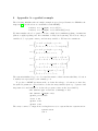
Remark. (about pictures from .dot file). It may be the case that the arcs connecting
two distinct nodes n1 and n2 with a father node n0 have the same label L: the meaning
is that the formula labelling n1 has been obtained by applying the same transition (on
the same variable) as that applied to obtain n1; the only difference is that cases of the
update-by-cases function have been applied in a different way.16 This situation can be
disambiguated by looking at how the nodes are created in the .report.tex file.
Nodes in gray are either subcovered or have been deleted by the backward redundancy
elimination heuristics. Recall that a node is subcovered [20] when it has an ascendant
node which has been deleted. In the abstraction/refinement mode (options -AN,-BN,
15
The dot format can be read by the GraphViz tool, which is available free for many platforms at the address
http://www.graphviz.org/. Using this tool you can export the graphs produced by MCMT in various format
(e.g. pdf) so that they can be included in latex documents.
16
Notice that this is well possible, because MCMT makes a backward search analysis (if read from backward,
the update function is not deterministic because it is the converse of a function).
20
-CN) such nodes do not contribute to the safety invariant and are basically considered
as deleted themselves.
4.3
Invariant search options
In this subsection, we list command line options that are related to a powerful MCMT functionality, namely invariant search. An important remark is in order here. By invariant we
mean in this document just trace invariant, i.e. any property which is enjoyed by all reachable
states. Full invariants (also called inductive invariants and sometimes simply ’invariants’ in
the literature) are properties which are enjoyed by the initial states and preserved by the
system evolution. When trying to prove a trace invariant, MCMT in fact completes it to a
stronger statement (which will be a full invariant) by disjoining it with further properties it
finds during its computations.
-i1 enable a minimal heuristic for invariant search. MCMT tries to find invariants consisting
of one universal quantifier followed by a disjunction of literals. In particular, it tries
to find invariants modelling the relationships between the values stored in the program
counter and the other local variables.
-i2 same as above, but invariants with two variables are searched for.
-i3 now both invariants with one and two variables are searched for.
-c enables abstraction of numeric constants arising in backward reachability search.
-a similar to -i3, but invariant search is now more aggressive, involves quantifier elimination
and abstracted indexes are projected away; this option may be combined with signature
abstraction (see Section 7).
-I same as “-i3 plus -c plus -a” (the latter with dynamic signature abstraction). It is the
most aggressive setting for invariant search: it gives MCMT more chances to find useful
invariants but at the same time it might considerably slow down the tool.
More information about invariant search will be supplied in Section 7.
4.4
Displayed information
If not run in silent mode, mcmt displays some information about heuristics, reachable states
formulae, trace invariants found, and statistics. We give here few explanations about node
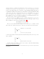
representation. The meaning of the displayed line
node19 = [t5 2 3][t6 2][t7 2][t6 1][t7 1][0]
21
(2)
is that mcmt is considering a formula describing a set of states that can reach an unsafe state
by executing transitions t5, t6, t7, t6, t7 in this order. In case all applied transitions
were specified in flat format, it is possible to deduce further information as explained below
(this is not the case however for non flat transitions if lazy flattening is applied, because
lazy flattening introduces at runtime the needed extra quantified variables). Formula (2) is
primitive differentiated and has three quantified variables, that is it is of the kind ∃z1 , ∃z2 ∃z3 ψ
(to see the formula, you must inspect either the Yices file produce by the option -y or compile
the Latex file produced by the option -r). It is possible to realize that the formula has three
quantified variables by the fact that 3 is the maximum number occurring in (2) following
an underscore. More precisely, to get an unsafe state from a state satisfying our formula
∃z1 , ∃z2 ∃z3 ψ one first applies transition 5 to z2 , z3 , then transition 6 to z2 , etc. (when we say
that transition 5 is applied to z2 , z3 , we mean that transition 5 has two exitentially quantified
variables x, y in its guard and that x is mapped to z2 whereas y is mapped to z3 ). Notation
(2) is rather informative, but it is slightly incomplete (even in case lazy flattening did not
occur) because it does not mention which case in the case-defined update functions applies to
each variable: displaying this information too would result in a rather cumbersome outcome,
so in case of ambiguity it is necessary to consult the full information supplied by files produced
by the options -y, -r.
The remaining messages displayed by mcmt should be self-explaining. We just point
out that mcmt supplies warnings for the only two cases where un unsafe outcome might be
spurious:
• the stopping failure model has been adopted (because of universal quantifiers in transition guards), hence the unsafety trace can in principle be good for the stopping failures
model but not good for the intended model;
• due to incomplete implementation, quantifier elimination of integer data variables occurring in the guards have been done imprecisely by overapproximating the set of backward
reachable states.
In particular, if neither universally quantified index variables (see Subsection 3.4) nor existentially quantified data variables (see Subsection 7.5) occur in the guards, unsafety traces
are not spurious.
In case an unsafe trace has been found, this means that the last displayed formula (2) is
consistent with the initial formula. To get an assignment describing a state that can reach an
unsafe configuration, run Yices with the option -e on the file .yices-log produced by the
mcmt option -y and take the last assignment displayed by Yices. In case a spuriousness risk
22
have been warned, it is possible to check spuriousness of the trace, but this can only be done
manually in the present release of the tool.
23
5
Abstraction/Refinement Mode
The main novelty of version 2.0 (and superior) is the support for abstraction/refinement loops.
This is based on predicate discovery via interpolation [20], as adapted to array-based systems
in [3]. In particular, interpolants are computed via abstraction over lists of terms (according
to the so-called term abstraction heuristics implemented also in SAFARI [4]); for the lack
of interpolants support in the background SMT-solver Yices, interpolants are computed via
some ad hoc form of quantifier elimination applied to fresh variables replacing the terms to
be abstracted away.
From the point of view of the user, to activate abstraction/refinement one needs to operate
on the command line and (optionally) also on the specification file. For command line, we
have three options.
-AN (where N is a natural number): this is the basic option, the number N puts a bound on
the number of times a node is refined (with N set to 0, a practically unlimited number of
refinements is applied, but refinement is applied in a lazy way). In practice, values like
N = 5, 6, . . . , 10 are recommended. Nodes are abstracted by eliminating terms in the
abstraction lists one after the other, until trace unsatisfiability persists. In presence of
an unsafe trace discovered during backward search, the abstraction operation is repeated
with more information, yieldying lighter abstractions: in this way a node can be refined
more and more.
-BN (where N is a natural number): this option is similar to the previous one; the difference
is that the covering test is here less aggressive (this option does not seem to give real
benefits).
-CN (where N is a natural number): this option produces an overhead aiming at making a
preliminary investigation about soundness of a proposed abstraction. If the proposed
abstraction is found to lead to a spurious unsafety trace, it is disregarded; if it leads to an
invariant, the tool adds it to its list of known invariants. If the preliminary investigation
about soundness of the proposed abstraction is inconclusive, the tool proceeds as with
option -AN. To explore soundness of proposed abstractions, the tool makes a copy of
itself with bounded resources, using the same resource parameter bounds as for invariant
search.
mcmt has its own default heuristics to generate term abstraction lists; this default heuristics (that basically includes symbolic parameters and global variables used as iterators) is
sufficient to solve basic problems, but for more difficult problems a human intervention is
24
desirable.17 The human intervention consists in introducing appropriate term abstraction
lists in the specification file. In case this happens, the default heuristics for generating such
lists is disabled automatically.
Term abstraction lists can be relative or absolute (the list generated by the default heuristics is absolute). Absolute lists are introduced in the specification file through the instruction
<term1> · · · <termk>
:term abstraction list
where <term1>,...,<termk> are terms. For instance
:term abstraction list
a length,
I, c[z1]
tells MCMT to abstract out, in the order, a length, I and c[z1] (here a length could be
a constant of type int introduced via a definition passed to the SMT solver). It is advisable
(although not mandatory) not to include in the list terms like a[z1] if a has been declared
to be local; index variables like z1 should also preferably not be included.
The instruction for relative lists is
:term abstraction list
N
<term1> · · · <termk>
where N is a natural number bigger than 0. The meaning of the above relative term abstraction
list is that it guides abstraction only for formulae that are obtained as preimages along the
transition number N (transitions are numbered as they are introduced in the specification file,
starting from 1). An absolute term abstraction list might coexist with some relative ones:
in that case, the absolute list applies to preimages along transitions for which there are no
relative lists.
It is possible to introduce in the specification file just one absolute empty term abstraction
list: this has the only effect that the tool keeps track of deleted subsumed nodes.
When the tool automatically builds term abstraction lists, it firsts includes in such lists
symbolic parameters (like array length, etc.) and then global array id’s. In some examples,
it is more useful to use the reverse ordering; the user can tell MCMT to apply the reverse
ordering by the instruction
:inverse term abstraction synthesis
Such istruction is used in some specifications from the distribution.
The instruction (available since version 2.5.2)
:term abstraction list
]global
produces a term abstraction list comprising all symbolic parameters and all global array
variables (except possibly the ‘program counter’, i.e. the global array variable number 1).
17
It should be pointed out that appropriate terms for term abstraction lists are usually terms already present
in the specification file and quite often the good combination is a relative combination of symbolic parameters
(like array lengths, etc.) and iterators. Thus, some parallel execution of different combinations obtained by
suitable heuristics is likely to get the right setting automatically, if such setting exists.
25
6
Acceleration
Acceleration, in the model checking terminology, is the computation of the transitive closure
of a transition. MCMT supports two limited forms of acceleration: the former applies to
integer variables, the latter to array variables. The former is a very weak version of wellknown formats for acceleration, the latter is peculiar to MCMT. Acceleration is activated as
follows. If you write
:accelerate transition n.
k
the system tries to accelerate the k-th transition. Integer acceleration is tried first and, in
case it fails, array acceleration is tried too. Writing
:accelerate all transitions you can
causes MCMT to try to accelerate all transitions; the same effect can be obtained through
the command line option -Z. The directive
:display accelerated transitions
forces MCMT to print on the screen the accelerated transitions it finds.
In case acceleration succeeds, the original transition is replaced by the accelerated one in
the integer acceleration case, whereas in the array acceleration case the accelerated transition
is just added to the set of the current transitions. The user is informed about the success
of the acceleration operation (nothing is said in case of failure). It is important to know
that MCMT can only accelerate single transitions in the present release: to accelerate cycles,
the user must manually compute the composite transition of the cycle, insert it as a further
transition in the specification file, and finally ask MCMT to accelerate it.
Another severe limitation comes from the fact that acceleration - as implemented in the
current release of MCMT - is quite rigid from the syntactic point of view: if the formats
described below are not strictly matched, the tool does not recognize acceleratability and
consequently ignores the acceleration suggestions.
6.1
Integer Acceleration
This form of acceleration can be useful for instance when analyzing Petri nets reachability:
the framework implemented in MCMT is roughly the same as that described in [9] (for good
updated information on acceleration in linear integer arithmetic, see [10]).
Integer acceleration succeeds in case: (i) the transition has zero or one existentially quantified index variable; (ii) only literals of the kind (>= a[x] N), (>= b N), (<= a[x] M), and
(<= b M) - where M, N are integers, a is a local array variable and b is a global variable occur in the guard; (ii) all local array variables a[j] are incremented/decremented by a constant value in the (= x j) case and left unchanged in the (not (j = x)) cases; (iii) global
26
variables are similarly incremented/decremented in all cases.
6.2
Array Acceleration
Array acceleration applies to local simple ground assignments in the terminology of [7]; we
give a description of what transitions MCMT considers local simple ground assignments. The
conditions are the following ones:
• the transition must have one or two update cases;
• the guard must contain a literal like (= x I), where I (the ‘iterator’) must be a global
variable of type int;
• all global variables must be updated identically, except I;
• except for the (not (= x j)) case, all local arrays must be updated identically;
• the update of the counter must be an increment (or a decrement) by one.
The acceleration of a local simple ground assignment contains universal guards [7], hence
by default it is treated according to the stopping failure model. However, accelerated transitions are in principle not needed to discover unsafety; MCMT knows it and consequently
treats the preimages computed via array accelerated transitions as abstractions (to be refined
to false) in case spurious traces arise. In order to maintain the data needed for uncovering,
MCMT automatically switch to abstraction/refine mode with empty terms abstraction lists
in case it succeeds in the array acceleration for at least one transition.18 Terms abstraction
lists won’t be empty however if abstraction/refinement is activated from command line; in
that case, the tool combines acceleration with abstraction and this powerful combination is
often essential to solve difficult problems.
6.3
User-Defined Accelerations
The ability of MCMT to recognize acceleratable transition is very rudimentary and often the
tool fails in this attempt for rather accidental ‘syntax-dependant’ reasons. Notice also that
there are quite simple acceleratable transitions that do no yet fit any ‘officially‘ known class
of acceleratable transitions. If the user realizes that a transition can be accelerated and that
the accelerated transition fits MCMT language - independently on the fact whether the tool
is able to realize it or not, it can include the accelerated transition in the specification file
using the keyword
18
This is a novelty of version 2.5.
27
:a transition
instead of :transition). In abstraction mode, the tool considers such transitions just as a
machinery to introduce abstractions, hence their applications are canceled every time they
originate spurious unsafety traces.
28
7
Advanced Settings
In this section we explain some important settings of MCMT that can be obtained by including
special instructions into the input specification file (sometimes such instructions must be
combined with appropriate command line options).
7.1
Bounds
Quite often, in sequential programs, iterators are used to scan the content of an array. In
these cases, some obvious invariants holds: for instance, the value of an iterator I is always
smaller than a symbolic parameter N expressing the size of the array, or it is bigger than
another iterator J, etc. These iterators are modeled via global array declarations; symbolic
parameters are introduced via :smt commands. The instruction
:determine bounds
causes MCMT to investigate whether such obvious invariants hold, via a bounded resource
invariants investigation. In case they hold, they are used in satisfiability tests and they are
also added to the guards of the relevant transitions to improve the quality of refinements (if
the tool is working in abstraction/refinement mode).
7.2
Interaction
MCMT allows some form of interaction. If you write in the input file
: suggested negated invariants
: var
z1
: var
z2
: cnj
<list-of-literals>
···
: cnj
<list-of-literals>
: end of suggested negated invariants
MCMT tries to prove the suggested invariants. In case it succeeds, it will use them later on
in all consistency tests. The lists of literals can contain at most the variables z1, z2.
Notice that if you want to check the universally quantified invariant ∀z1 ∀z2 C (where C is a
clause) you must enter the literals corresponding to the negation of C. The universal closures
of the negations of the formulae you enter need not be inductive invariants: MCMT will try by
itself to complete them to inductive invariants (e.g. if you enter a property which refers to a
29
precise location, MCMT will propagate it automatically to other locations, if needed). Hence
the :suggested negated invariant block of instructions is particularly useful to insert code
annotations in the specification files. To this aim, notice however that there is an alternative
choice, namely that of using multiple unsafe states descriptions (see the :u cnj keyword,
Section 3): the two choices are declaratively but not procedurally equivalent. In the case
of suggested negated invariants, MCMT tries to check the suggested invariants one after
the other, with bounded resources: in case it does not succeed or it only partially succeed,
it will nevertheless proceed to the task of verifying the unreachability of the main unsafe
configuration. On the contrary, in case of multiple unsafe states descriptions, it will check
unreachability of the declared unsafe configurations all together (and will report unsafety in
case at least one of them is reachable).
7.3
Bounded Resources in Invariant Search
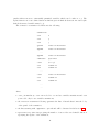
When trying to check that a candidate invariant is indeed a true (trace) invariant, MCMT
has only bounded resources at its disposal. This is because invariant synthesis can be expensive and can easily fail. The user can modify these resources by specifying his preferred
bounds in the input file (these user defined bounds will be used in all the command line
options involving invariant search, namely -i1, -i2, -i3, -c, -a, -I, -CN as well as in
the :suggested negated invariant block of instructions above). The following table summarizes the directives about resource bounds in invariant search that can be introduced in
the input MCMT specification files:
Directive
Def. Value
Explanation
: inv search start N
[def N=0]
begin invariant search
after node N
: inv search max index var N
[def N=5]
no more than N variables
can arise in invariant search
: inv search max num nodes N
[def N=150]
no more than N nodes
can arise in invariant search
: inv search max num invariants N
[def N=200]
find at most N invariants
: inv search max num cand invariants N
[def N=500]
try at most N candidate
invariants
Notice that if the preassigned bounds are not sufficient, search is interrupted and the
candidate invariant is discarded.
The directive
: inv search only candidates
30
asks MCMT to generate candidate invariants without checking (and hence without using)
them. This can be useful (in combination with the command line options -dN, -e) in shell
scripts running many copies of MCMT in parallel.
7.4
Signature Abstraction
Predicate abstraction is a powerful technique in model checking. The current release of MCMT
implements it in full CEGAR style. A more primitive (but still useful) abstraction technique
inherited from older versions of the tool is still available and works as follows. MCMT can
project (during invariant search) the candidate invariants it finds and their preimages over a
subsignature indicated by the user. This restricts the search and enhance the possibility of
finding good invariants.
To specify the abstract signature, type
: abstract signature
: subsignature
k
: subsignature
l
: subsignature
m
···
: end of abstract signature
in the input file. Here k, l, m, ... are either 1 or 0 depending on the fact you want or
you do not want the corresponding array to be abstracted away (you have one line per array,
following the array variables declaration order). Writing just
:dynamic signature abstraction
you leave MCMT to find automatically the closest signature for abstraction when examining
each candidate invariant.
Notice that all the above directives about signature abstraction are effective only when
combined with the command line otions -a, -I.
7.5
Elimination of quantified variables
To model real-time systems in the timed automata style, existentially quantified (real, integer)
variables for data may be used in guards. These variables are not envisaged in primitive
differentiated formulae, hence they must be eliminated.
Existential variables to be eliminated are introduced in MCMT as follows. First, before
writing any transition, you must declare such variables as
31
:eevar <char> <type-id>
where <char> is a single character (the name of the existentially quantified variable) and
<type-id> is either real or int (in case the type specification is missed, the variable is
assumed to be real).
The name of the existentially quantified (integer, real) variable is thus fixed for all the
transitions; you can declare both an integer and a real variable, but they should have different
names and cannot be used in the same transition together. Existentially quantified integer
or real variables must occur only in atoms written in the language of linear arithmetic and
they are not allowed in negative literals.19
Once the preimage of the formula representing a set of states is computed, the real variable
is eliminated by using Fourier Motzkin quantifier elimination. As to the integer variable,
the situation is more complex because MCMT does not support yet full integer quantifier
elimination. The procedure applied instead is the following. First, integer literals like (< t
u) are replaced by (<= (+ t 1) u). After that, Fourier Motzkin is used: the user is informed
that the set of backward reachable states obtained in this way is overapproximated and, in
case an unsafe trace is found, he is warned once again about the fact the trace could be
spurious because of overapproximation. Notice however that in some trivial cases, Fourier
Motzkin and integer quantifier elimination agree: in such cases, there is no overapproximation
at all and no overapproximation warning is displayed.
Overapproximations of integer quantifier elimination are employed during invariant search
too: however, no warning is displayed there because invariants are fully checked before being used (in other words, the overapproximation may cause the failure of the synthesis of
some invariant, but does not affect the correctedness of the final MCMT outcome). Similarly, quantifier elimination due to accelerated transitions may cause overapproximation;
again, this does not cause troubles because the tool shifts automatically in this case to the
abstraction/refinement mode, where spurious traces are detected and eliminated.
Remark. MCMT uses the character ’@’ for internal quantifier elimination operations, so
this character should not be used in specification files; it may happen that MCMT ask the
user to define an :eevar (even in case it may not really use it), if it feels that the default
names he has for such variables may conflict with user-defined id’s.
7.6
Cardinality bounds
If a parametrized problem looks too difficult, one can try to verify it in special cases by
imposing a cardinality bound on the sort INDEX. This cannot be done by a system axiom (by
19
This is not a real expressivity limitation, because instead of a guard containing, say (not (= e a[x])),
you can write two transitions containing only <=, <, >=, > in their guards.
32
internal implementation reasons), but there is the possibility of specifying such a bound in
the input file by typing
:max domain cardinality N
where N is a number like 3, 4, 5, etc. (do not use values greater or equal to 10, because
the tool exits automatically when he realizes he needs more than 10 variables to solve the
problem, hence a value bigger than 10 would have no practical effect).
7.7
Key search
We made little experiments on using MCMT in planning problems. It seems that there are a
couple of options that could be useful in such contexts (but it is rather obvious that MCMT
would need substantial enrichment to perform well on such problems). First of all, one can
disactivate forward redundancy tests for formulae describing backward reachable sets of states
by typing
:no backward simplification
in the input file. A much more useful option seems to be the possibility of classifying the
formulae describing backward reachable sets of states (whenever possible) according to the
value of a global variable. This can be achieved by typing
:key search g
in the specification file (here g should be a previously declared global array variable). If the
list of the formulae describing backward reachable sets of states is quite big, this strategy
alllows a more efficient access to that list during fixpoint tests.
7.8
Variable redundancy
Despite the fact that MCMT is quite optimized in this sense, it is sometimes possible that
redundant existential variables are produced during backward search: such variables could be
easily eliminated in case they have an explicit definition of the kind ∃zi (zi = t ∧ · · · ). MCMT
can be forced to look for the possibility of such elimination by the directive
:variable redundancy test
Notice that this variable elimination procedure is always precise (it does not cause overapproximations), but may occasionally have undesired consequences on heuristics for invariant
search, especially in presence of global array variables.
In abstraction/refinement mode it might happen that variables previously eliminated cannot be eliminated anymore after a refinement: in such cases, MCMT adopts the drastic
solution of rebuilding from skratch the search tree below the node that caused the problem.
33
7.9
Static limits
There is a static limitation on the maximum number of array variables allowed (raised to 100
since version 2.1). However the user can set by himself the maximum number of transitions
by including the instruction
:max transitions number N
in the specification file. Notice that the upper bound N (set to 50 by default) should include
also accelerated transitions that might be produced by the tool itself. In case more than N
transitions are specified or generated by acceleration, an error message is displayed.
7.10
Restricted Instantiation
One of the key features of MCMT is full quantifier handling; this requires full instantiation,
in the sense that quantified variables are instantiated in all possible ways during satisfiability
tests (instantiations are optimized by powerful but nevertheless complete heuristics). Full
instantiation prunes search space dramatically, but can be expensive. For this reason, the
user is given the possibility of limiting it, especially in the final phases of the backward search
computation. Typing in the input file
:flex fix point fixed index var
N
:flex fix point active node number
M
and using the option -f from the command line, the standard algorithm of MCMT is modified
as follows. After node M has been reached, the first N variables are always instantiated identically in satisfiability tests for fixpoints. If values for M, N are not given in the specification
file and the command line -f is used, MCMT employs the default values M=2 and N=50.
7.11
Memory reset
For difficult problems, it empirically turns out to be useful to reset the SMT solver from time
to time, in order to prevent out of memory runs. This is achieved by the following directives:
Directive
Def. Value
Explanation
: start reset N
[def. N=375]
after N nodes the SMT solver is
periodically reset ...
7.12
: reset ratio M
[def. M=75]
... with ratio M
: intensive reset P
[def. P=30000]
after P nodes the ratio becomes 1
Channels
In the present release, MCMT does not support many-dimensional arrays. This is a severe
limitation, we show here how to indirectly circumvent it in some cases. In many distributed
34
system specifications, communication channels arise: in these specifications, one can express
for instance the fact that process p has sent an ack to process q by saying that ack is the
location of the channel with source p and target q. If it is implicitly assumed that there is
a communication channel between any two processes whatsoever, the most natural modeling
of this setting would employ 2-dimensional arrays, but as we said MCMT does not support
them. We explain here the formalization we used in some examples of the distribution:
this formalization produces models which are slightly more general than the intended ones,
however they seem to behave properly in the applications.
The idea is that the type INDEX is reserved to channels; channels have a source and a
target and processes are identified with channels whose source and target coincide. To get
this, it is sufficient to introduce two free function symbols20
:smt (define S::(-> nat nat))
:smt (define T::(-> nat nat))
We need to know whether an index variable refers to a process or to a channel. To this
aim, we introduce a unary predicate P (for “being a process”) and leave the system axiom
: smt
(define P::(-> nat bool))
: system axiom
: var
x
: cnj
(= (P x) (= (S x) (T x)))
to define it appropriately. Another system axiom says that targets and sources are processes
and not channels
: system axiom
: var
x
: cnj
(and ((P (S x)) (P (T x)))
A further system axiom might be used in case we want to ensure that channels having
the same source and target are identical:
20
Alternatively, one could introduce two local arrays with values in the type nat and never update them in
the transitions.
35
: system axiom
: var
x
: var
y
: cnj
(=> (and (= (S x) (S y)) (= (T x) (T y))) (= x y) )
As claimed above, this setting represents an approximation of 2-dimensional arrays which
should be sufficient to address safety problems in specifications involving channels. We expect
that a future direct implementation of 2-dimensional arrays will produce considerable gain
both in expressivity and in efficiency.
36
8
Appendix A: a guided example
The following ‘initialize-and-test’ simple example is quoted as problematic for CEGAR techniques in [18] (we show how we can handle it with MCMT):
for(I=0; I!= a length; I++) a[I]=0;
for(J=0; J!= a length; J++) assert(a[J]==0);
We first translate the above pseudo-code into a high level formalism speaking of transitions
(this is, roughly speaking, into the formalism of array-based systems). We need two integer
variables I, J, a program counter p and an array variable a. We have five transitions:

τ1 = 
τ2
τ3
τ4
τ5
p = 1 ∧ I < a length ∧ p0 = 1 ∧


I 0 = I + 1 ∧ J 0 = J ∧ a0 = wr(a, I, 0);


p = 1 ∧ I ≥ a length ∧ p0 = 2 ∧

=
0
0
0
I = I ∧ J = 0 ∧ a = a;


p = 2 ∧ J < a length ∧ a[J] = 0

=
0
0
0
0
p = 2 ∧ I = I ∧ J = J + 1 ∧ a = a;


p = 2 ∧ J < a length ∧ a[J] 6= 0

=
p0 = 4 ∧ I 0 = I ∧ J 0 = J ∧ a0 = a;


p = 2 ∧ J ≥ a length ∧ p0 = 3 ∧

=
I 0 = I ∧ J 0 = J ∧ a0 = a;
The system is initilized by p = 1 ∧ I = 0 and the unsafe condition is unreachability of location
4, namely it is represented by the formula p = 4.
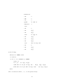
To produce a MCMT specification file, we define the subtype of locations, we introduce
the symbolic parameter a length and we declare the array variables (it is a good practice and
important for some heuristics to declare the program counter as the first variable):
:smt (define-type locations ( subrange 1 4))
:smt (define a length::int)
:global p locations
:local a int
:global I int
:global J int
The array a cannot be empty, hence its length is not 0; we express this via a system axiom:
:system axiom
:var x
37
:cnj (< 0 a length)
We now introduce initial and unsafe formulae:
:initial
:var x
:cnj (= I 0) (= p 1)
:unsafe
:var z1
:cnj (= p 4)
Our transitions are written as follows (we exploit the possibility of writing them in a non flat
form):
: comment Tau1
: transition
: var j
: guard
(= p 1) (< I a length)
: numcases 2
: case (= j I)
: val p
: val 0
: val (+ I 1)
: val J
: case (not (= I j))
: val p
: val a[j]
: val (+ I 1)
: val J
38
: comment Tau2
: transition
: var j
: guard
(= p 1) (>= I a length)
: numcases 1
: case
: val 2
: val a[j]
: val I
: val 0
: comment Tau3
: transition
: var j
: guard
(= p 2) (< J a length) (= a[J] 0)
: numcases 1
: case
: val p
: val a[j]
: val I
: val (+ J 1)
: comment Tau4
: transition
: var j
: guard
(= p 2) (< J a length) (not (= a[J] 0))
: numcases 1
: case
: val 4
: val a[j]
: val I
: val J
39
: comment Tau5
: transition
: var j
: guard
(= p 2) (>= J a length)
: numcases 1
: case
: val 3
: val a[j]
: val I
: val J
Finally, for specification files formalizing imperative programs using iterators to scan arrays,
it is advisable to use the heuristics
:variable redundancy test
in order to avoid the introduction of redundant existentialy quantified variables.
Our specification file is now ready. If we run MCMT without options, the tool clearly
diverges; static invariant generation or static abstraction options (like -I, -a) seem not to
help. Thus, we must rely on abstraction mode and/or on acceleration.
Let us try first with abstraction mode; the options -A5, -B5 (or similar) seem inconclusive;
option -C5 solves the problem and certifies safety, but it takes a while to conclude (about
10-15 sec. on a standard laptop). We’ll see how to get good performances with acceleration
below. For the moment, let us point out that if we want more information from the tool, we
can use options
-C5
-v0
-S4
together. Thanks to option -v0, we get a file status.txt reporting exit data and MCMT
prints on the screen (the negation of) the invariant it found. Such invariant is logically
equivalent to the expected one, namely
p 6= 4 ∧ (p = 1 → ∀z (z < I → a[z] = 0)) ∧ (p = 2 → ∀z (z < a length → a[z] = 0))
(3)
(notice that such invariant contains a universally quantified variable). The option -S4 makes
the formulae written by the tool much more readable (it is an aggressive semantic redundancy
test for literals), but it might produce a considerable overhead, like in our case.
Let’s now consider aceleration. To make aceleration effective, one usually has to compute
compound cycles and insert them in the specification file as further transitions (such procedure
40
can be automatized, but it is not even partially implemented in the current release). Our
case is lucky, because transitions 1 and 3 are already a cycle that can be accelerated. If we
run MCMT with option -Z, the tool certifies safety in negligible time (much less than one
second). To get the (negation of the) safety invariant displayed on the screen and to produce
the status file, we can use the options
-Z
-v0
-S4
together (since the problem is solved instantaneously, the time overhed caused by the option
-S4 is negligible in this case). The invariant displayed on the screen in our case is an involved
formulation of a condition that turns out to be just a slight variant of (3) above.
To complete the picture, one can also try the combined options:
-Z
-A5
-Z
-C5
which are both able to instantaneously solve the problem. As a further remark, notice that
if we add the instruction
:determine bounds
in the sepecification file, the tool correctly realizes that in location 1 the iterator I must not
exceed a length and in in location 2 the iterator J must not exceed a length; this information
is used during backward search, but the problem is too easy for this to give a real benefit.
In this example, it seems that acceleration is the winning strategy. However this is only
due to the fact that the default abstraction list produced automatically by MCMT is not the
good one: if one reverses it (via the instruction :inverse term abstraction synthesis),
one gets immediate success with plain abstraction -A5 without acceleration!
It should be pointed out, as a general remark, that the behavior of the different settings
of MCMT turns out to be rather irregular on significant examples; sometimes, a combination
of acceleration and abstraction is the best way to handle problems where divergence is the
main source of troubles (see [7] for an experimental discussion and see also the comments
included in the specification files of the distribution). The most promising strategy seems to
be that of trying in parallel different settings and different heuristics for the generation of
terms abstraction lists.
41
References
[1] P. A. Abdulla, G. Delzanno, N. B. Henda, and A. Rezine. Regular model checking
without transducers. In TACAS, volume 4424 of LNCS, pages 721–736, 2007.
[2] P. A. Abdulla, G. Delzanno, and A. Rezine. Parameterized verification of infinite-state
processes with global conditions. In CAV, volume 4590 of LNCS, pages 145–157, 2007.
[3] F. Alberti, R. Bruttomesso, S. Ghilardi, S. Ranise, and N. Sharygina. Lazy Abstraction
with Interpolants for Arrays. In LPAR-18, pages 46–61, 2012.
[4] F. Alberti, R. Bruttomesso, S. Ghilardi, S. Ranise, and N. Sharygina. SAFARI: SMTbased Abstraction For Arrays with Interpolants. In CAV, 2012.
[5] F. Alberti, S. Ghilardi, E. Pagani, S. Ranise, and G. P. Rossi. Universal guards, relativization of quantifiers, and failure models in model checking modulo theories. To appear
in Journal on Satisfiability, Boolean Modeling and Computation (JSAT). Available at
http://homes.dsi.unimi.it/~ghilardi/allegati/AGPRR_JSAT.pdf.
[6] F. Alberti, S. Ghilardi, E. Pagani, S. Ranise, and G. P. Rossi. Brief announcement:
Automated support for the design and validation of fault tolerant parameterized systems
- a case study. In DISC 10, LNCS, 2010.
[7] F. Alberti, S. Ghilardi, and N. Sharygina. Definability of Accelerated Relations in a
Theory of Arrays and its Applications. In FroCoS, 2013. Also available as Technical
Report, Universit`
a della Svizzera Italiana.
[8] F. Alberti, S. Ghilardi, and N. Sharygina. Decision Procedures for Flat Array Properties.
In TACAS, 2014. Also available as Technical Report, Universit`a della Svizzera Italiana.
[9] B. B´erard and L. Fribourg. Reachability Analysis of (Timed) Petri Nets Using Real
Arithmetic. In CONCUR’99, LNCS, pages 178–193, 1999.
[10] M. Bozga, R. Iosif, and F. Konecny. Fast acceleration of ultimately periodic relations.
In CAV, LNCS, 2010.
[11] A. Carioni, S. Ghilardi, and S. Ranise. MCMT in the Land of Parametrized Timed
Automata. In Proc. of VERIFY 10, 2010.
[12] A. Carioni, S. Ghilardi, and S. Ranise. Automated Analysis of Parametric Timing-Based
Mutual Exclusion Algorithms. In NASA Formal Methods, LNCS, 2012.
42
[13] S. Ghilardi, E. Nicolini, S. Ranise, and D. Zucchelli. Towards SMT Model-Checking of
Array-based Systems. In Proc. of IJCAR, LNCS, 2008.
[14] S. Ghilardi and S. Ranise. Goal-directed Invariant Synthesis for Model Checking Modulo
Theories. In TABLEAUX’09, LNCS, 2009.
[15] S. Ghilardi and S. Ranise. Model Checking Modulo Theory at work: the intergration of
Yices in MCMT. In Proc. of AFM’09, ACM Digital Library, 2009.
[16] S. Ghilardi and S. Ranise. Backward reachability of array-based systems by SMT-solving:
termination and invariant synthesis. Logical Methods in Computer Science, 6(4), 2010.
[17] S. Ghilardi, S. Ranise, and T. Valsecchi. Light-Weight SMT-based Model-Checking. In
Proc. of AVOCS 07-08, ENTCS, 2008.
[18] R. Jhala and K.L. McMillan. Array Abstractions from Proofs. In CAV, 2007.
[19] Nancy A. Lynch. Distributed Algorithms. Morgan Kaufmann, 1996.
[20] K. L. McMillan. Lazy Abstraction with Interpolants. In CAV, 2006.
43