Download A∗ Wars: The Fight for Improving A∗ Search for Troubleshooting

∗
∗
A Wars: The Fight for Improving A Search
for Troubleshooting with Dependent Actions
Thorsten J. Ottosen and Finn V. Jensen
Department of Computer Science
Aalborg University
9220 Aalborg, Denmark
Abstract
Decision theoretic troubleshooting combines Bayesian networks and cost estimates to obtain optimal or near optimal decisions in domains with inherent uncertainty. We use the
well-known A algorithm to nd optimal solutions in troubleshooting models where different actions may x the same fault. We prove that a heuristic function proposed by
Vomlelová and Vomlel is monotone in models without questions, and we report on recent
work on pruning. Furthermore, we experimentally investigate a hybrid approach where
A is combined with a method that sometimes avoid branching. The method is based on
an analysis of the dependency between actions as suggested by Koca and Bilgiç.
can be used for models with questions, but since
1 Introduction
model without questions does not lead to
Imagine that you have a device which has been aAND-nodes
the search tree, we only need to
running well up to now, but suddenly it is mal- consider the insimpler
A algorithm (Hart et al.,
functioning. A set of faults F describes the pos- 1968) (Dechter and Pearl,
1985) for models with
sible causes to the problem. To x the problem dependent actions.
you have a set A of actions, which may x the We can summarize our troubleshooting asproblem and a set Q of questions, which may sumptions as follows:
help identifying the problem. Each action or Assumption 1. There are no questions.
question S has a positive cost C (ε) possibly
depending on evidence ε. Your task is to x the Assumption 2. There is a single fault present
problem as cheaply as possible. In this paper we when troubleshooting begins. (This implies that
do not consider questions.
we can have a single fault-node F with states
When actions in a model can remedy sets of f ∈ F .)
faults that overlap, we say that the model has Assumption 3. Actions are conditionally independent actions. Finding an optimal solution dependent given evidence on the fault node.
in models with dependent actions is of great Assumption 4. The cost of actions C (ε) is
practical importance since dependent actions independent from evidence ε.
can be expected to occur in many non-trivial domains. However, all non-trivial troubleshooting We use the following notation. The model
scenarios have been shown to be NP-hardthis provides for all A ∈ A and f ∈ F probabiliincludes models with dependent actions (Vom- ties P(f | ε) , P(A | ε) and P(A | f), where ε is evilelová, 2003).
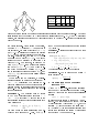
dence. In Figure 1 is shown a simple model with
Two dierent approaches have previously dependent actions. We have some initial evibeen used for nding optimal strategies: (Jensen dence ε , and in the course of executing actions
et al., 2001) describes a branch & bound algo- we collect further evidence. We write ε to de(ε ⊆ ε ),
rithm whereas (Vomlelová and Vomlel, 2003) de- note that the rst i actions have failed
scribes an AO algorithm. The AO algorithm and we have by assumption P ε = 1 because
∗
∗
∗
S
i
A
0
i
0
∗
∗
0
i
F
f1
f2
A1
f3
f1
f2
P(a1 | F)
P(a2 | F)
P(a3 | F)
P(F)
CA1
CA2
CA3
1
0
0
0.20
= =
f4
A2
f3
1 0
1 1
0 1
0.25 0.40
=1
f4
0
0
1
0.15
A3
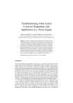
Figure 1: Left: a simple model for a troubleshooting scenario with dependent actions. The dotted
lines indicate that the faults f to f are states in a single fault node F. A , A and A represent
actions, and parents of an action node A are faults which may be xed by A. Right: the quantitative
part of the model.
1
4
1
the device is faulty. When action A has failed,
we write A = ¬a whereas A = a means that it
has succeeded. We often abbreviate P(A = ¬a)
as P(¬a). The presence of the fault f is written
F = f , but we often abbreviate the event simply as f. Furthermore, we write P(ε ∪ f) when
we really had to write P(ε ∪ {f}). The set of
faults that can be repaired by an action A is
denoted fa (A). For example, in Figure 1 we
have fa(A ) = {f , f }. In models where actions
can have P(a | ε) = 1, fa (·) is a dynamic entity which we indicate by writing fa(· | ε). The
set of remaining actions is denoted A(ε), and
A (f | ε) ⊆ A(ε) is the set of remaining actions
that can x f.
When there are no questions, a troubleshooting strategy is a sequence of actions s =
hA , . . . , A i prescribing the process of repeatedly performing the next action until the
problem is xed or the last action has been performed. To compare sequences we use the following denition:
Denition 1. The expected cost of repair
(ECR) of a troubleshooting sequence s =
hA , . . . , A i with costs C is the mean of the
costs until an action succeeds or all actions have
been performed:
2
2
2
3
the ECR for an optimal sequence of the actions
A(ε) given ε .
Example 1. Consider a sequence for the model
in Figure 1:
ECR (hA2 , A3 , A1 i) =
CA2 + P(¬a2 ) · CA3 + P(¬a2 , ¬a3 ) · CA1
= CA2 + P(¬a2 ) · CA3
+ P(¬a2 ) · P(¬a3 | ¬a2 ) · CA1
7
7 4
= 1+
·1+
· · 1 = 1.55 .
20
20 7
3
A crucial denition is that of eciency:
Denition 2. The eciency of an action A
given evidence ε is
ef(A | ε) =
P(A = a)
.
CA (ε)
2 Monotonicity of the heuristic
function ECR
A (and AO ) is a best-rst search algorithm
that works by continuously expanding a frontier node n for which the value of the evaluation
function
f (n) = g(n) + h(n),
(1)
is minimal until nally a goal node t is expanded. The cost between two nodes n and m
(m reachable from n) is denoted c(n, m), and the
X
ECR (s) =
C (ε ) · P ε
.
function g(n) is the cost from the start node s
to n whereas h(n) is the heuristic function that
We then dene an optimal sequence as a se- guides (or misguides) the search by estimating
quence with minimal ECR. Also, ECR (ε) is the cost from n to a goal node t.
1
1
n
n
Ai
n
Ai
i−1
i−1
i=1
∗
∗
∗
If h(n) ≡ 0, A degenerates to Dijkstra's algo- Not only is ECR(·) easy to compute, it also
rithm. The cost of the shortest path from s to has the following property (Vomlelová and Vomn is denoted g (n), and from n to t it is denoted
lel, 2003):
h (n). Finally, the evidence gathered about
Theorem 1. Under Assumption 2-4 the heurisactions from s to n is denoted ε (ε ⊆ ε ).
tic function ECR(·) is admissible, that is,
Denition 3. A heuristic function h(·) is adECR(ε ) ≤ ECR (ε ) ∀ε ∈ E.
missible if
For a class of heuristic functions, A is guaranh(n) ≤ h (n) ∀n .
teed
found the optimal path to a node
When A is guided by an admissible heuristic whentothehave
node
is expanded (Hart et al., 1968):
function, it is guaranteed to nd an optimal soDenition 5. A heuristic function h(·) is monolution (Hart et al., 1968).
(Vomlelová and Vomlel, 2003) have sug- tone if
gested the following heuristic function for use
h(n) ≤ c(n, m) + h(m),
in troubleshooting:
whenever m is a successor node of n.
Denition 4. Let E denote the set containing
all possible evidence. The function ECR : E 7→ Remark. Monotonicity is equivalent to the often
used and seemingly stronger consistency propR is dened for each ε ∈ E as
X
erty: h(n) ≤ c (n, m) + h(m) ∀n, m.
ECR(ε ) = P(ε ) ·
P(f | ε ) · ECR (ε ∪ f) .
Henceforth we let A denote the performed
Remark. In (Vomlelová and Vomlel, 2003) the action on the edge from a node n to a successor
factor P(ε ) is left out. However, the factor node m in the search graph.
ensures that the decomposition in Equation 1 Proposition 1. For the heuristic function
takes the simple form
ECR(·) under Assumption 1 and 4 monotonicity
∗
∗
∗
n
0
n
∗
n
n
n
∗
∗
∗
+
n
n
n
∗
n
∗
n
n
f∈F
n
is equivalent to
f (n) = ECR (εn ) + ECR(εn ) ,
| {z } | {z }
g(n)
ECRh (εn ) ≤ CAn + P(¬an | εn ) · ECRh (εm ) .
h(n)
where ECR (ε ) is the ECR for the sequence Proof. We have c(n, m) = P(ε ) · C and
dened by the path X
up to n. We also dene
P(ε ) = P(¬a | ε ) · P(ε ) and so the common
ECR (ε) =
P(f | ε) · ECR (ε ∪ f) .
factor P(ε ) cancels out.
The optimal cost ECR (ε ∪ f) is easy to cal- Theorem 2. Under Assumption 1-4 the heurisculate under Assumption 2-4: the optimal se- tic function ECR(·) is monotone.
quence is found by ordering the actions in
A (f | ε ) with respect to descending eciency
Proof. The idea is to express ECR (ε ) in
(Kadane and Simon, 1977).
terms of ECR (ε ). To do that we consider
Example 2. Assume the fault f can be repaired the complement of the set fa(A ) which is the
by two actions A and A and that P(a | f) = set of all faults that A cannot x. For each
f ∈ F \ fa(A ) Bayes' rule (conditioned) yields
0.9 and P(a | f) = 0.8. Furthermore, let both
actions have cost 1. Since instantiating the fault
1 · P(f | ε )
node renders the actions conditionally indepen,
P(f | ε ) =
P(¬a | ε )
dent, P(a | ε ∪ f) = P(a | f) and the eciencies
of the two actions are 0.9 and 0.8, respectively. because P(¬a | ε ∪ f) ≡ 1. If we restrict
We get
ECR (·) to a subset of faults X , we shall abuse
ECR (ε ∪ f) = ECR (hA , A i)
notation and write it
n
n
m
∗
n
n
An
n
n
h
f∈F
∗
n
n
h
h
n
m
n
1
2
n
1
n
2
n
m
n
n
∗
n
n
h
1
2
= CA1 + P(¬a1 | f) · CA2
= 1 + 0.1 · 1 = 1.1 .
ECRh (ε | X) =
X
f∈X
P(f | ε) · ECR∗ (ε ∪ f) .
In particular, we must have
By Proposition 1, we have to prove ∆ ≤ C .
of Bayes' rule and Assumption 3 we
(2) Because
have
| fa(A )).
An
n
ECRh (ε ) =
ECRh (εn | F \ fa(An )) + ECRh (εn
We can furthermore dene
n
= ECRh (εm | F \ fa(An ))
∆F
− ECRh (εn | F \ fa(An )) ,
P(¬an | εn ) · P(f | εm ) =
P(¬an | f) · P(f | εn )
P(¬an | εn ) ·
P(¬an | εn )
= P(¬an | f) · P(f | εn ) .
which is an extra cost because all faults in F \ So we get
X
fa(A ) are more likely. Similarly
∆=
n
∆fa(An ) =
ECRh (εm | fa(An )) − ECRh (εn | fa(An )) ,
P(f | εn ) ·
f∈fa(An )
∗ n
[ECR (ε ∪ f) − P(¬an | f) · ECR∗ (εm ∪ f)] .
|
{z
}
is the cost lost or gained because A has been
performed and can no longer repair the faults Because of the single-fault assumption, we only
fa(A ). We can then express ECR (ε ) by
need to prove that δ ≤ C . We now index the
actions in A (f | ε ) as follows:
ECR (ε ) = ECR (ε ) + ∆fa(A ) + ∆F, (3)
P(B
= b | f)
P(B = b | f)
The constant ECR (·) factors implies
≥
∀i.
C
C
X
∆F =
[P(f | ε ) − P(f | ε )] · ECR (ε ∪ f).
In this ordering, we have A = B . The inequalities generalizes to
Exploiting Bayes' rule (as explained above) and
P(B = b | f)
Equation 2 we get
C ≤
·C
∀j > i .
(4)
P(B = b | f)
∆F
=
In particular, this is true for j = x which we
− 1 · ECR (ε | F \ fa(A )) =
shall exploit later.
h
i
ih
Assume we have N dependent actions in
−1 · ECR (ε )−ECR (ε | fa(A )) .
A (f | ε ). The rst term of δ is then
Inserting into Equation 3 yields
ECR (ε ∪ f) = ECR (hB , . . . , B i)
ECR (ε ) = ECR (ε ) +
X
Y
= C +
C ·
P(¬b | f) .
(5)
ECR (ε | fa(A )) − ECR (ε | fa(A ))
δ
n
n
m
h
m
h
An
n
n
n
h
∗
i
m
∗
n
i+1
i
Bi
n
Bi+1
n
f∈F \fa(An )
Bi
1
P(¬an | εn )
h
1
P(¬an | εn )
h
n
n
m
n
h
+
n
h
Bj
∗
B1
n
i
1
−1
·
P(¬an | εn )
h
i
n
n
ECRh (ε )−ECRh (ε | fa(An ))
h
ECRh (εn )
=
+ ECRh (εm | fa(An ))
P(¬an | εn )
1
−
· ECRh (εn | fa(An )),
P(¬an | εn )
and we rearrange the equation into
n
ECRh (ε |fa(An ))−P(¬an|ε )·ECRh (ε |fa(An )).
|
{z
}
N
j
Bi
j=1
Assume that x > 1 (we shall deal with x = 1
later), then the second term of δ is
P(¬an | f) · ECR∗ (εm ∪ f) =
P(¬an | f) · ECR∗ (h. . . , Bx−1 , Bx+1 , . . .i)
= P(¬an | f) ·
x−1
i−1
h
X
Y
CB1 +
CBi ·
P(¬bj | f)
i=2
m
1
i−1
i=2
ECRh (εn ) = P(¬an | εn ) · ECR(εm ) +
∆
j
N
n
n
j
n
h
m
i
n
n
n
h
i
x
n
∗
h
i+1
PN
+
j=1
i=x+1 CBi
·
Qi−1
j=1 P(¬bj | f)
P(¬an | f)
i
.
We see that the last term is also represented in as required. This is not surprising if we look at
Equation 5 and therefore cancels out. We get the expression inside the parenthesis of Equation 6: the corresponding events are "B xes f,
δ = C · [1 − P(¬a | f)] +
B xes f if B did not x f " etc. up to "none of
X
Y
the actions xed f". These events form a sample
[1 − P(¬a | f)] ·
C ·
P(¬b | f)
space.
When x = 1, then δ = C − P(¬a | f) · C ,
Y
so
in all cases δ ≤ C which completes the
+C ·
P(¬b | f) ,
proof.
It is quite straightforward to show that
where the last term is a leftover from Equation Remark.
ECR(·) is not monotone when the model in5. Using P(¬a | ε) = 1 − P(a | ε) and Equation cludes questions.
4 we get
3 Pruning based on eciency and
δ = C · P(a | f) +
ECR
X
Y
We recently investigated the eect of a prunP(a | f) ·
C ·
P(¬b | f)
ing method based on eciency (Ottosen and
Jensen, 2008). By considering two adjacent
Y
actions in an optimal troubleshooting sequence,
+C ·
P(¬b | f)
the following has been proved about the eciency (Jensen et al., 2001):
P(b | f)
· C · P(a | f) +
≤
1
n
x−1
B1
2
1
i−1
n
j
Bi
i=2
j=1
An
x−1
n
An
An
j
An
j=1
n
B1
x−1
n
i−1
j
Bi
i=2
j=1
x−1
j
An
j=1
1
n
A
n
P(an | f)
x−1
i−1
X
Y
P(bi | f)
P(an | f) ·
· CAn ·
P(¬bj | f)
P(an | f)
i=2
Let s = hA1, . . . , Ani be an optimal sequence of actions with independent costs.
Then it must hold that
Theorem 3.
j=1
+ CAn ·
x−1
Y
ef(Ai | εi−1 ) ≥ ef(Ai+1 | εi−1 ),
for all i ∈ {1, . . . , n − 1}.
P(¬bj | f)
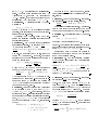
In Figure 2 it is illustrated how the theorem
can be used for pruning. If we have the order
· P(b | f) +
ef(A ) > ef(A ) > ef(A ) at the root, we know
X
Y
that A should never be the rst action. FurP(b | f) ·
P(¬b | f)
thermore, after performing A , we know that A
should never be the second action. We call this
i
Y
pruning.
+
P(¬b | f)
(6) eciency-based
In summary, the theorem was very easy to exploit during the expansion of a node by keeping
h
· 1 − P(¬b | f) +
the actions sorted with respect to eciency and
by passing that information in the parent node.
(1 − P(¬b | f)) · P(¬b | f)
However, the results where a bit disappointing
i
Y
since it only gave a speed-up of a factor of 2-4.
+··· +
P(¬b | f)
We have since then tried to extend the idea
h
by considering three adjacent actions instead of
· 1 − P(¬b | f) · P(¬b | f)
two. We call this ECR-based pruning. Figure
2 shows an overview of the pruning process. If
i
Y
+··· +
P(¬b | f)
we consider an arbitrary subset of three actions
A , A , and A , we would normally need to compare six dierent sequences. However, if we have
· 1,
j=1
= C An
h
1
1
x−1
2
i−1
3
i
j
i=2
2
j=1
x−1
j
j=1
= C An
1
2
x−1
1
j
j=1
= C An
2
1
x−1
j
j=1
= C An
3
1
2
3
1
calculated the eciencies of the three actions
at the local root node with evidence ε, Theorem 3 leaves us with only three possible candidates. After the three sequences are expanded,
the paths are coalesced into a single node in the
search graph.
Now imagine that A is about to expand A
in the sequence hA , A , A i. We determine
if the current node expansion is optimal by
comparing it with the ECR of the sequence
hA , A , A i. (There is no need for comparing
hA , A , A i with hA , A , A i since Theorem 3
has pruned the latter.) If we expand the sequence hA , A , A i rst, the analysis is similar
and we compare with the best of the two other
sequences (again, the best sequence is found by
applying Theorem 3).
There is no way to avoid calculating the full
ECR of both sequences, and we have to traverse
the search graph down to the root and up to
the rst node of the second path. Furthermore,
this traversal means that we have to store child
pointers in all nodes, and we also need to keep
all expanded nodes in memory. This more than
doubles the memory requirement.
In conclusion the method turned out to slow
down A . In a model with 19 action and 19
faults, Theorem 3 pruned 989k nodes whereas
the ECR-based pruning prevented a mere 3556
expansions out of about 41k possible.
Theorem 2 also explains why the eect of the
pruning is so small: if A is guided by a monotone heuristics and expands a node, then the optimal path to that node has been found (Hart et
al., 1968). This means that the sub-trees outlined with dotted edges in Figure 2 are never
explored unless we really need to explore them.
Should we discover a non-optimal sequence rst,
that path is not explored further until coalescing
happens.
4 An A hybrid approach
Troubleshooting with dependent actions was
proved NP-hard by reduction from the exact
cover by 3-sets problem (Vomlelová, 2003).
Therefore, troubleshooting in models where
each action can repair three or more faults is
∗
2
3
1
1
2
3
2
3
ε
A1 A2
A3
3
1
2
3
1
3
2
A2 A3
A3
A3
A2
A1
A1
1
∗
Figure 2: An overview of the pruning process for
any subset of three actions. At the root of the
subtree we have evidence ε and the actions are
sorted with respect to eciency, and we have
ef(A | ε) > ef(A | ε) > ef(A | ε). Theorem 3
implies that we can prune the nodes ending in a
square, and so we are left with only three possible sequences (hA , A , A i, hA , A , A i, and
hA , A , A i). After A has discovered the last
node in these three sequences, the three paths
are subject to coalescing.
1
2
3
1
2
3
1
2
∗
3
1
3
2
∗
∗
NP-hard. However, A still has diculties in
nding a solution for models with much lower
average dependency (that is, the average size of
fa(·) over all actions). Remarkably enough, we
found that when the average dependency went
down from 3 towards 1, then the running time
increased many times. In the following we describe a hybrid method for models with an average dependency well below 3.
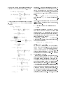
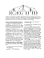
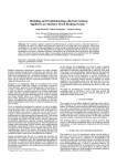
Figure 3 shows an example of the search tree
explored by A in our hybrid approach. Near the
root node, A is often forced to create a branch
for each successor node. However, as we get
closer to the goal nodes, branching is more likely
to be avoided. The branching can be avoided
∗
∗
∗
Figure 3: An example of what the search tree looks like in our hybrid approach. For some nodes,
the normal A branching is avoided, and near goal nodes this branching is almost avoided for all
nodes. We can see that it might happen that the algorithm has to investigate all successors of a
node even though the path down to that node was explored without branching.
∗
because we are able to determine the optimal
next step of the remaining sequence (see below).
This leads us to the following denitions:
Denition 6. A dependency graph for a troubleshooting model given evidence ε is the undirected graph with a vertex for each action A ∈
A(ε) and an edge between two vertices A and
A if fa(A | ε) ∩ fa(A | ε) 6= ∅.
Denition 7. A dependency set for a troubleshooting model given evidence ε is a connectivity component in the dependency graph given ε.
Denition 8. A dependency set leader for a
troubleshooting model given evidence ε is the
rst action of an optimal sequence in a dependency set given ε.
Dependency sets are important because the
order of actions in the same dependency set does
not change when actions outside the set are performed. This property has been exploited in the
following theorem (Koca and Bilgiç, 2004):
1
2
1
2
Suppose we are able to calculate
the dependency set leaders. Then the globally
optimal sequence is given by the following algorithm:
1. Construct the dependency sets and retrieve
the set leaders.
2. Calculate ef(·) for all set leaders.
Theorem 4.
3. Select the set leader with the highest ef(·)
and perform it.
4. If it fails, update the probabilities, and continue in step (2).
Our hybrid approach then simply works by
nding the optimal sequence in dependency sets
of a fairly small size. For this work we have restricted us to sets of a size < 4. At any point
before expanding a node, if the most ecient
action belongs to a dependency set of such a
small size, we nd the rst action in that dependency set. If the dependency set consists of
one or two actions, this calculation is trivial. If
the dependency set has three actions, we nd
the rst by comparing the three candidate sequences as we discussed in Section 3. Otherwise
we simply expand the node as usual by inspecting all successors.
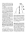
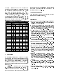
Table 4 shows the results of three versions
of A . We can see that the hybrid approach
is somewhat slower for models with an average
dependency between 2 and 3. This is because
the hybrid approach spends time investigating
the size of the dependency set of the most efcient action, but it rarely gets to exploit the
benets of a small dependency set. For an average dependency between 2.1 and 1.6 the hybrid
approach becomes superior, and below 1.6 it becomes very fast.
∗
Table 1: Results for the hybrid approach in
models with 20 actions and 20 faults. The average dependency ranges between 3 and 1, and
each action is usually associated with 1 to 3
faults. The time is measured in seconds. "A " is
A with coalescing, "pruning-A " is "A " plus
eciency-based pruning and "hybrid-A " is the
hybrid approach based on "pruning-A ". Already at an average dependency around 2.1 we
see that the hybrid method wins.
Method
A pruning-A hybrid-A
Dep.
Time
3.0
33.56
11.48
12.27
2.9
42.11
12.42
21.97
2.8
62.14
15.08
27.52
2.7
45.03
14.38
21.61
2.6
29.86
10.20
12.39
2.5
86.52
22.20
29.61
2.4
31.55
12.39
12.00
2.3
65.19
19.11
21.28
2.2
80.56
21.28
29.38
2.1
50.28
18.72
9.78
2.0
83.75
27.70
20.05
1.9
62.88
16.77
10.64
1.8
127.59
35.09
18.72
1.7
102.17
25.36
14.42
1.6
133.17
39.14
25.41
1.5
122.08
27.59
0.92
1.4
164.84
41.16
4.25
1.3
139.89
39.44
0.13
1.2
168.42
38.13
0.00
1.1
160.42
39.42
0.00
1.0
159.95
38.08
0.00
∗
∗
∗
∗
∗
∗
∗
∗
∗
5 Discussion
We originally investigated Theorem 2 because
monotonicity plays an important role in promising bidirectional A methods (Kaindl and Kainz,
1997). However, a bidirectional A for troubleshooting is very dicult because there is no apparent way to start a search from the goal nodes
using ECR(·).
The hybrid A approach seems very promising. We still need to determine how large a dependency set that it pays o to solve. We expect that it will be most benecial to solve small
∗
∗
∗
dependency sets by brute-force whereas dependency sets of medium size can be solved by a
recursive call to hybrid-A .
Acknowledgements
We would like to thank the reviewers for their
valuable and detailed feedback.
∗
References
Rina Dechter and Judea Pearl. 1985. Generalized
best-rst search strategies and the optimality af
a*. J. ACM, 32(3):505536.
P. E. Hart, N. J. Nilsson, and B. Raphael. 1968.
A formal basis for the heuristic determination of
minimum cost paths. IEEE Trans. Systems Science and Cybernetics, SSC-4(2):1007.
Finn V. Jensen, Ue Kjærul, Brian Kristiansen,
Claus Skaanning, Jiri Vomlel, and Marta Vomlelová. 2001. The sacso methodology for troubleshooting complex systems. Articial Intelli-
gence for Engineering Design, Analysis and Manufacturing, 15:321333.
J. Kadane and H. Simon. 1977. Optimal strategies for a class of constrained sequential problems.
The Annals of Statistics, 5:237255.
Hermann Kaindl and Gerhard Kainz. 1997. Bidirectional heuristic search reconsidered. Journal
of Articial Intelligence Research, 7:283317.
Eylem Koca and Taner Bilgiç. 2004. A troubleshooting approach with dependent actions. In
Ramon López de Mántaras and Lorenza Saitta,
editors, ECAI 2004: 16th European Conference
on Articial Intelligence, pages 10431044. IOS
Press.
Thorsten J. Ottosen and Finn V. Jensen. 2008.
Better safe than sorryoptimal troubleshooting
through A* search with eciency-based pruning.
In Proceedings of the Tenth Scandinavian Conference on Articial Intelligence, pages 9297. IOS
Press.
M. Vomlelová and J. Vomlel. 2003. Troubleshooting: Np-hardness and solution methods. Soft
Computing Journal, Volume 7, Number 5, pages
357368.
Marta Vomlelová. 2003. Complexity of decisiontheoretic troubleshooting. Int. J. Intell. Syst.,
18(2):267277.