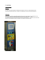
1
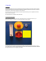
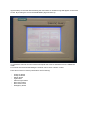
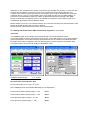
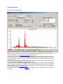
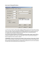
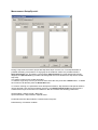
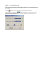
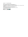
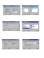
•
•
•
•
XRF Core Scanner User Manual
XRF Core Scanner Program, Getting Started
XRF Core Scan Program, Default Values
Winaxil Batch, Getting Started
•
•
•
External Connections XRF Core Scanner
Canberra Connections XRF Core Scanner
Canberra X - PIPS / DSA 1000
Installation and Configuration
XRF Core Scanner user manual version 2.0
(C) N.I.O.Z. & Avaatech 20/08/2007
Table of contents
Section
1
1.1
1.2
2
2.1
3
3.1
3.2
3.3
3.4
3.5
4
4.1
4.2
4.3
4.4
Title
Page
General information
3
Description of the XRF core scanner
Overview of the main components
3
4
Installation
5
Requirements
5
Operation
6
Warning
Functional description
Sample preparation
Data acquisition
Data processing
6
6
11
11
12
Appendices
13
Specifications
Trouble shooting
Material information sheet for Beryllium
Radiation safety data sheet
13
15
16
17
WARNING
The X-rays generated in the source are dangerous and may be fatal if encountered. Extreme caution
must be exercised when working with this equipment. Radiation dosimeters must be worn by anyone
working with or observing the operation of this equipment.
Purchasers planning to install a radiation machine should ensure they are in compliance with local,
state and federal regulations.
CAUTION X – RAYS.
This Equipment Produces High Intensity X-Ray Beams When Energized.
To Be Operated Only by Qualified Personnel.
See appendix 4.4 for a radiation safety data sheet.
1. General information
1.1 Description of the XRF core scanner
The XRF (X-Ray Fluorescence) Core Scanner is originally designed for rapid and non- destructive
determination of the chemical composition of marine bottom sediments onboard ships and at
laboratories ashore. Marine bottom sediments are often sampled by means of box-cores, gravity-cores
and piston-cores, and collected in plastic tubes which are subsequently split in length.
The XRF measurements are carried out on split cores.
As an example, the XRF core scanner is able to perform a complete scan of a one meter long core
with a sample resolution of 1 cm within 30 minutes or faster.
This gives the possibility to take a new core in the same area if the chemical data show that the core
does not contain the expected information or that errors were made with coring.
The core scanner is equipped with a motor actuated door that gives access to the core fit system. The
core fit system can fit a split core by mechanical system. The XRF analysis method requires an X-ray
source and detector to be positioned accurately above the sediment surface. Therefore a computer
controlled positioning system positions the core and the instruments accurately even if the core is not
cut very homogeneously.
Instead of a split sediment core other sample holders can be fitted and measured in the scanner. For
example samples on a microscope-glass can be measured without problems. The demand for proper
XRF analysis is a horizontal surface.
The data acquisition of a core is carried out on a personal computer. Before a scan, all positions or
areas of interest are entered. The scanning of a core is computer controlled. If the scanner cannot find
a sediment surface it will continue with the next position.
Post-processing of the data is carried out on the same computer.
1.2 Overview of the main components
The XRF core scanner consists of five main parts:
1) Core scanner with DC motor actuated X- and Z-axis, stainless steel bearings for Z-axis,
stainless steel X-ray safe enclosure with X-ray safe window for visual inspection, electric
motor driven door and mechanical core fitting.
2) Intelligent scanner electronics with precise positioning capabilities, integrated safety interlock
mechanism, programmable logic control with touch screen for fault-finding and manual control
functionality.
3) Forced air-cooled Oxford 100 Watt X-ray source with Rhodium anode and a voltage range of
4...50 kV and current range of 0…2 mA.
4) Canberra X - Pips 1500-1.5 Detector: 8 mm² collimated to 5 mm², crystal thickness 1.5 mm
Be-window: 0.5 mil ( soldered, coated) Canberra DSA 1000 ( MCA )
5) Personal computer running under Windows XP with fully automated data acquisition and
processing software.
Note:
Both the X-ray source and the X-ray detector contain Beryllium windows as an
X-ray transparent separation between vacuum and atmospheric conditions.
Beryllium is a toxic material!
2. Installation
2.1 Requirements
Electricity:
The XRF core scanner needs one electrical connection to a 230 V / 50 - 60Hz mains net. The
connection should be fused with 16 Ampere. See appendix 4.1 for the electrical specifications.
Helium gas:
Helium gas is necessary during XRF-measurements. It has a much lower X-ray absorption then air.
The helium pressure at should be adjusted with a pressure regulator at 0.5…1 bar.
The required helium flow during XRF-measurements is approximately 10…30 ml/min at environmental
pressure. The estimated live time of a 200 bar / 50 l bottles is around 200 days.
3. Operation
3.1 Warning
The X-rays generated in the source are dangerous and may be fatal if encountered. Extreme caution
must be exercised when working with this equipment. Radiation dosimeters must be worn by anyone
working with or observing the operation of this equipment.
Purchasers planning to install a radiation machine should ensure they are in compliance with local,
state and federal regulations.
See appendix 4.4 for a radiation safety data sheet.
3.2 Functional description
Before switching on the core scanner the compressed air from an external air source, e.g. a
compressor should be connected. The helium gas bottle must be opened.
The MAIN SWITCH mounted on the left side of the XRF Core-Scanner must be switched to position
“ON”. Always push the button RESET EMERGENCY STOP after activating the main switch; otherwise
the system will remain in an emergency stop status.
Approximately 30 seconds after activating the main switch an Avaatech logo will appear on the touch
screen. By touching the screen the MAIN MENU page will show up.
To operate the scanner from the Personal Computer the scanner should be set in the ‘REMOTE’
mode.
For scanner service and fault finding the scanner can be set to ‘LOCAL’ control.
From this moment on various push buttons are functioning:
-
X-Ray On button
X-Ray Off button
Helium button
Light button
Camera Light Button
Door Open button
Door Close button
Emergency button
Only when the safety-interlock circuit is activated it is possible to produce X-rays.
The door can only be opened when the X-rays are switched off.
The interlock lamp (green) is lit when the safety-interlock circuit is activated. This indicates that all
doors are closed and locked.
-
Set key switch LOCK to ON, the standby lamp (white) is lit
Push the black X-RAY ON button to activate X-ray tube
The X-RAY ON lamp (yellow) is lit, also the lamps on top of scanner is lit
Push the red X-RAY OFF button to switch off the X-ray tube
-
The HELIUM button opens a valve that enables a helium flow to the X-ray detection area. The
flow meter must be adjusted to 10…30 ml/min. A mass flow meter measures the actual helium
flow and causes a warning message on the data acquisition computer when the helium flow is
below 5 ml/min.
-
The LIGHT SCANNER button activates the spot lights inside the scanner.
The LIGHT CAMERA activates the linear light source of the camera system.
-
The DOOR OPEN button opens and the DOOR CLOSE button closes the door that gives access
to the core fit section of the scanner. When the cover closes care must be taken for hands and
fingers. For safety reasons the cover is locked when in closed position.
The door can only be opened when the X-rays are switched off.
Warning:
If the air-cooled X-ray tube was operated at maximum power it is recommended to keep the door
closed for 5 minutes after switching off the X-rays. This enables the X-ray tube to cool down and
avoid the activation of the thermal fuse of the tube.
See section 4.2, trouble shooting, for more details.
-
Pressing the EMERGENCY STOP button immediately stops any scanner or door movement and
switches off the X-ray tube. To recover from an emergency stop pull the emergency stop button
out and press the RESET EMERGENCY STOP button. To recover from an emergency stop also
press the RESET ERROR and RESET CYCLE buttons at the touch screen. These buttons are
available on the Main Menu screen.
3.3 Sample preparation
To prevent contamination of the helium flushed measurement triangle the surface of the sediment core
is covered with a very thin Ultralene foil (appr.4µm thick).
X-ray fluorescence analysis gives chemical information of only the upper tens of micrometers of the
sample. Therefore it is important to avoid any form of contamination.
When the Ultralene foil is applied, air-bubbles can be enclosed between the sample and foil. These
air-bubbles must always be removed because they absorb X-rays and influence the data quality.
X-ray fluorescence analysis demands a flat and homogeneous surface. Sometimes it is necessary to
carefully smoothen the sediment surface after the foil has been applied. This can be done using a roll
of tape by rolling it gently from one side to the other. Always be careful not to contaminate the surface.
3.4 Data acquisition
Before the data acquisition can start two important settings must be chosen.
1) count time :
how many seconds to measure at each position
The count time setting is a trade-off between data quality and scanning speed. Values between 10 s
and 60 s are most common.
2) X-ray excitation
:
which kV, mA and filter settings are appropriate
In general for the best results of K-line analysis a combination with certain kV and mA values can be
applied :
a)
b)
c)
d)
e)
no filter is used for Al up to Fe, at about 10 kV
an Al filter for S up to Mn, 10 to 20 kV
a thin Pd filter for Ti up to Ge, 10 to 25 kV
a thick Pd filter for Fe up to Mo, 20 to 40 kV
a Cu filter for Zr up to Ba, at about 30 to 50 kV
For heavier elements than Ba the L-lines are used for analysis.
For pragmatic reasons, such as lack of time, combinations of elements will be measured that will give
reasonable results with one filter/kV combination. A few examples:
1) Al up to Fe can be measured without filter at 10 kV. Al up to Ti gives than good results. Mn
and Fe, however, are counted somewhat less effectively. Sr cannot be measured at this kV.
2) If Mn and Fe are important they are most effective measured at 12 kV with the cellulose or the
Al filter. Ti and lower elements will then be measured less effectively.
3) Mn and Fe can also be measured at 20 kV applying with the cellulose or Al filter. Sr will then
be measured fairly.
4) Sr and Zr can be measured well at 30 kV using a thick Pd filter.
5) For Ba 50 kV and the maximum mA must be used in combination with the Cu filter.
Further, it is a matter of trial to find the optimum conditions for a combination of elements. In case
these conditions can not be found in one filter/kV combination the samples must then be measured at
two or more conditions.
The X-ray current setting depends on the average composition of the sample. To set the current to its
optimal value it is important to understand the principle of ‘dead-time’.
‘Dead-time’ considerations:
The X-rays emitted by the sample are detected and processed by the detector and its electronics. The
processing speed of the electronics is limited. Therefore the amount of X-rays entering the detector is
limited. Dead-time is a percentage that indicates the amount of time that is needed for processing. A
dead-time of 40% indicates that only 60% of the time X-rays actually are counted. To correct for this
the time-base is delayed. A count time of 30 s with a dead-time of 40% will actually take 50 s.
A higher current setting, meaning a higher X-ray intensity, gives a higher dead-time thus increased
measuring times. A very low current setting gives a low dead-time but also poor data statistics. In
practice it is recommended to adjust the current so that the dead-time percentage is 10…50%.
During the scanning of a sediment core it is not allowed to change the current setting anymore. It
would disturb the linearity of the qualitative results.
Before starting a scan, the core name and length, the count time and step size must be entered. Also
special areas with another step size can be entered.
During the scan a XRF spectra is stored for each measurement.
See Getting started manual for XRF Core Scanner Program for more details.
3) Slit size
The irradiated length of the sample can be adjusted with a motor-controlled slit system.
The slit size setting should be set using the touch-screen on the XRF-Scanner. From the main Menu
press the Slit button. On the Slit screen the desired slit-size can be entered in the Destination field.
Press the GoTo button to adjust the slit. The final slit opening can be read from the Position field.
The arrow buttons can be used to modify the Destination value.
Irradiated sample length:
0.1…10 mm
See main menu Touch Screen SLIT
By the small steps ( from 1 mm – 0.1 mm )
GoTo 2 mm and than Goto with 0.1 mm steps to your adjustment
Push left arrow button (above) steps + I mm
GoTo
Push left arrow button (under) steps – 1 mm
GoTo
Push right arrow (above) steps + 0.1 mm
GoTo
Push right arrow (under) steps – 1 mm
GoTo
Irradiated sample width:
2 - 15 mm
Huberslit
Turn Right = Close
Turn left = Open
One turn is turning the knob van 0 – 10
1 turn = 2 mm
2 turn = 4 mm
3 turn = 6 mm
4 turn = 8 mm
5 turn = 10 mm
6 turn = 12 mm
7 turn = 14 mm
7.5 turn is maximum
=15 mm
3.5 Data processing
The stored XRF spectra need to be processed to obtain X-ray intensity data. Processing consists of
subtracting a background curve, applying statistical corrections for physical processes in the detector
and deconvolution of overlapping peaks. After that the peak integrals are calculated and stored.
See Getting started manual for WinAxilBatch for more details.
4. Appendices
4.1 Specifications
Mechanical:
Weight:
Dimensions:
1225 kg
W = 340 cm, D = 80 cm H = 170 cm with door closed
H = 220 cm with door open
Electrical:
Input voltage:230 V AC Input frequency:50 / 60 Hz
XRF Core-Scanner/computer and electronics:
2500 W
Gasses:
Pressure:
Helium (type: 4.6) bottle 50 l/200 bar:
0.5…1 bar
X-ray generation:
Voltage range:
Current range:
Anode type:
Tube-sample filters:
4 ... 50 kV
0 ... 2 mA
Rhodium
Al – Pd Thin - Pd Thick - Cu
Irradiated sample length:
0.1…10 mm
Irradiated sample width:
2 - 15 mm
X-ray detection:
Multi Channel Analyzer:
FWHM @ 5.9keV better then:
2048 channels @ 20 eV/Ch
190 eV
X-ray shielding and safety:
Shielding materials :
Stainless steel, 8 mm thick in direct beam area, 3 mm thick for indirect excitation shielding.
Lead / PMMA alloy window, 25 mm thick
Safety mechanism:
Automatic safety interlock circuit with a 'first switch off X-rays, then open door' philosophy. The
door can only be opened after switching off the X-rays manually. Door is locked when X-rays
are switched on.
The X-rays can only be switched on manually after an automatic check of all safety
switches and status of the cover and service door locks.
The X-rays ON warning lights (near X-Ray ON switch, on top of scanner) are “FAIL SAVE”. If
a light bulb is broken, the X-rays can not be switched on.
Sample dimensions:
Allowable core length:
30 ... 160 cm
Allowable core width:
50 ... 130 mm
Scanner positioning:
X-direction:
Range:
Accuracy:
0 ... 160 cm
+/- 0.003 mm
Z-direction:
Repeatability:
0.05 mm or better
XRF analysis:
Detection limits of some elements:
Measured at 10kV, no filter and at 30 sec. count time:
Detection limits Avaatech XRF Core – Scanner
The estimated detection limits for 20 sec.counting time for a typical muddy sediment sample is:
Al...0.2%
Si...0..1%
P...0.05%
S....0.05%
K....0.04%
Ca..0.02%
Ti..0.05%
Mn..100 ppm
Fe..45 ppm
Sr...5 ppm
Zr..20 ppm
Ba….40 ppm
Measured at 50 kV, 1 mA, Cu filter and 30 sec. Count time, 1500µm detector:
Ba 200 ppm. (At 100 sec. count time this is somewhat lower)
4.2 Trouble shooting
Problem:
Action:
The X-rays can not be switched on.
The safety interlock circuit detects an unsafe situation. Check that the cover and
service doors are closed and locked. If the cover is closed, push down the cover into
its lock. Check safety switches of the cover and service doors. Check emergency
button. Check both X-rays ON light bulbs on top of scanner and miniature light bulb on
front panel.
Problem:
Action:
The X-rays can not be switched on.
The X-ray tube can be over-heated when used for a longer period on maximum
power. There is a thermal fuse on the outside of the X-ray tube. Press the red button
of the thermal fuse when the tube has cooled down.
Press RESET ERROR and RESET CYCLE on Main Menu of touch screen
Problem:
Action:
The cover will not open.
The X-rays are switched on. Check if emergency button is not activated.
Problem:
Action:
Emergency button has been activated.
To recover from an emergency stop pull the emergency stop button out and press the
RESET EMERGENCY STOP button.
Press RESET ERROR and RESET CYCLE on Main Menu of touch screen
Problem:
Action:
X-ray detector has been pushed upwards.
This generates an emergency stop situation. If the cause of the detector movement is
a serious crash of the detection triangle please contact AvaaTech immediately. If the
detector moved by accident recover from the emergency stop situation as described
above.
Problem:
Action:
Fault message 'X/Z Axis error' on display.
The X/Z-table did not reach the target position. Check for mechanical
obstructions. The scan must be restarted.
Problem:
Action:
No Helium bubbles in water bottle.
Open the Helium bottle.
Problem:
Action:
No Helium bubbles in water bottle, there is maybe a leak in foils of the prism
Remove the prism, and put new foil on the prism
4.3 Material information sheet for Beryllium
4.4 Radiation safety data sheet
Getting Started manual 1 for XRF Core Scanner Program 2
Version 3.0
August 2007
Bob Koster
Contents:
Part 1:
Introduction to the XRF Core Scanner Software
Part 2:
Launch Program
Startup Window
Part 3:
User Interface
Scanner Menu
View Menu
Setup Menu
Help Menu
Application Toolbar Buttons
Spectrum Toolbar Buttons
Statusbar
Part 4:
Part 5:
Instrument Settings and Measurement Setup Description
Spectrum Processing
Spectrum File Format
Using Canberra’s WinAxil for Processing
Part 6:
How Do I …
Connect to Scanner
Start a Step Scan
Start a Calibration Scan
Start a Stability Scan
Reset a scanner error on the touch screen
1
2
Contents of this manual is based on the Windows help files supplied with the XRF Core Scanner Software
XRF Core Scanner was developed by the Royal Netherlands Institute for Sea Research and exclusively
distributed and supported by AvaaTech Analytical X-Ray Technology
Part 1
Introduction to the XRF Core Scanner Software
Introduction:
The XRF Core Scanner Program is a multi-threaded application that runs on a personal computer with
a WIN32 based operating system, like WinXP and Win2000, and connects to the XRF Core Scanner
and to all of its scientific instruments.
The program controls all the instrument settings via the Instrument Settings window and can perform a
XRF scan on a split sediment core. A core position description, the X-Ray excitation and
measurement parameters are to be defined in the Measurement Setup window.
If a split sediment core has been put in the XRF Core Scanner the user needs to perform two things
over which the program has no control.
1) Push the Helium switch to flush the measurement chamber with helium.
2) Push X-Ray ON switch to start the X-Ray tube.
From here the program can perform a fully automated scan over the core and store the measured
XRF spectra in the chosen data directory.
At a later stage the acquired and saved spectra are to be processed with a separate processing
package.
Part 2
Launch Program
Launch Program:
The main screen looks like this:
At the top of the screen there is the main menu. Almost all the selectable items from the main menu
are also accessible via the Application Toolbar buttons below it.
In the upper-left corner there is a Scanner Status Panel that shows various parameters as a scan
proceeds. In the upper-right corner there is a Messages Panel that shows the various communication
commands between computer, detector and scanner. This panel can be useful to locate the sources
of possible errors.
Below there is an X-Ray Tube Status Panel that shows the actual X-Ray tube status. These values
are only updated if the program is connected to the scanner.
The largest panel is the Spectrum Display Panel. The live acquired spectrum is always displayed in
red. At any given moment an older spectrum can be read from disk and displayed as an overlay in the
Spectrum Display Panel. The appearance of the spectra in the Spectrum Panel can be manipulated
with the buttons from the Spectrum Toolbar.
At the bottom of the screen there is a Statusbar that shows spectrum related parameters as the scan
proceeds.
Part 3
User Interface
Scanner Menu:
The Scanner Menu contains two items :
Connect
Hardware
Exit
Connects program to scanner and its instruments
Control Direct control of scanner, X-Ray tube and detector
Terminates the program
View Menu:
The View Menu contains three items :
Scanner Messages
Detector Messages
None
Shows the logged messages from the scanner
Shows the logged messages from the X-ray detector
Setup Menu:
The Setup Menu contains two items :
Instrument Settings
Measurement Setup
Contains settings related to scanner
Contains settings related to the measurement
See part 6 for detailed description of setup screens.
Help Menu:
The Help Menu contains two items :
Help Contents Start the Win Help program with the contents tab selected
About
Shows an about box with company information
Application Toolbar:
Connection button
Instrument Settings button
Measurement Setup button
Scan Mode selector
Start Scan button
Stop Scan button
Spectrum Toolbar:
Select Linear or Logarithmic vertical scale
Display a stored spectra with different colors
Remove overlaid spectra from screen only
Make a hard copy of the Spectrum Display Panel
Move, Shrink and Expand spectrum horizontally
Expand and Shrink spectrum vertically
Auto-Scale spectrum vertically and horizontally
Status bar:
Position:
Total CPS:
Acquisition:
Live Time:
Real Time :
Dead Time:
Energy Intensity(*):
Current X-position of the scanner in [mm]
Total count per second counted by the multi channel analyzer
Status of Multi-Channel Analyzer [On/Off]
Elapsed Live time of current measurement in [s]
Elapsed Real time of current measurement in [s]
Percentage of Dead time in detection circuit in [%]
Cursor values in [keV] and [Counts]
(*) See also Energy Calibration parameters on Instrument Settings window
Part 4
Instrument Settings
&
Measurement Setup
&
Window description
Instrument Settings/Excitation:
To set an X-Ray excitation condition adjust the kV and mA sliders with the left mouse button pressed
at the correct value. Select the appropriate CountTime(*) and Filter between X-Ray tube and sample.
If the new excitation condition will often be used it could be added to the pre-defined excitation list.
The contents of the pre-defined excitation list can be cleared with the corresponding buttons.
An excitation list can be saved to or loaded from disk.
This pre-defined excitation list appears in the Measurement Setup window. There one can make a
choice which excitation condition is to be used for a step-scan. Even all excitation conditions from the
pre-defined excitation list can be chosen. That will result in a multi-run step scan that measures a
specific sample with various excitation conditions.
(*)CountTime is the time that the Multi-Channel Analyzer takes to acquire a spectrum. Since the MCA
is programmed to measure in 'live-time' the actual time a measurement takes is calculated as [Count
Time / (1- Dead Time/100%)], where Dead Time is a physical MCA phenomenon that is related to the
total counts that enter the X-Ray detector. The Dead Time is displayed on the main screens statusbar.
The Dead Time can be influenced by the X-Ray tube current.
Instrument Settings/Spectrum Display:
Both Energy Calibration settings Offset and Gain are implemented to transform the spectrum channel
numbers, in the Spectrum Display Panel, into energy values. The settings on this screen are only to
calculate the displayed energy value of the cursor in the Spectrum Display Panel. This energy value is
displayed in the right corner of the statusbar.
The measured and stored raw-data spectra are not affected by this display energy calibration.
Since the used spectrum post-processing package works with pre-defined processing models it is
strongly advised to have the hardware detector gain always set to the same value. Recommended
values are 20eV/Channel at 2048 channel spectra or 10eV/Channel at 4096 channel spectra.
Instrument Settings/Scanner:
The General settings Sample Offset and Safety Margin are implemented to calibrate the scanners Xposition and to prevent the scanner from measuring too close to the cores edges. The Sample Offset
is the distance between the scanners homing-switch and the "0 cm" location of the core to be
measured. Adjust this value if the mechanical "0 cm" position has been changed.
The Stability Scan settings Position, Max.Test Cycles and Re-position determine the behavior of a
stability scan. A stability scan repeatedly measures the same position on a core to check the systems
(and samples) stability. A stability scan ends automatically after the number of cycles set at Max.Test
Cycles. If the Reposition checkbox is checked the scanner re-positions before a measurement. If not
checked the scanner positions only once before the first measurement and then repeats the
measurements without any mechanical movements. The spectrum file name automatically contains a
cycle number. The excitation condition and data file directory are to be set in the Measurement Setup
window.
The Calibration Scan settings Position and Data File Path determine the behavior of a calibration
scan. A calibration scan is meant to monitor the systems long-term stability. At regular time intervals
the user can measure a reference sample that usually is positioned at the left side of the scanners "0
cm" position. This position is entered as an absolute positive value in millimeters counted from the
scanners homing-switch. The reference sample at such a location can be permanently available for
monitoring.
The Data File Path is the directory were the spectra are stored and overrules the usual data directory
path. This helps to collect all the long-term monitoring spectra at one central location. The spectrum
file name automatically contains the time and date of the measurement.
The excitation condition is to be set in the Measurement Setup window and should always be the
same !!!
Instrument Settings/Com Ports:
The scanner requires a serial COM port on the computer. The Scanner port setting determine which
port number physically connects to the appropriate device. If a settings is changed the program
should be re-connected to the scanner in order to activate the new settings.
Measurement Setup/Basic:
The Data Directory is the directory where the spectrum files, acquired during a scan, are saved in. By
pressing the Change … button an existing directory can be chosen or a new directory can be created.
Sample Name is the name of the core that is to be measured. Do not use any of the following
characters since they could give problems in Windows file names: [ . , / \ * ' " : ; ]
Sample Length is the exact length of the core. Step Size is the distance between each measurement
during a step scan. A [Special positions apply] sign next to the Step Size parameter indicates that
special positions apply for this scan. See Special tab topic for an explanation.
The Excitation condition to be applied can be chosen from the Instrument Settings / Excitation tab or
from the pre-defined excitation list. Even all excitation conditions from the pre-defined excitation list
can be chosen. That will result in a multi-run step scan that measures a specific sample with various
excitation conditions.
For loading and saving Measurement Scripts see Special tab topic for an explanation.
Measurement Setup/Special:
During a step scan the scanner jumps with Step Size steps over the core. To anticipate better on
possible interesting core positions or huge gaps in the sediment surface it is possible to define
Special Positions (e.g. in between a normal step), Skip Positions (a normal step that should be
skipped) and Special Areas (a possible interesting area where one would like to step with a smaller
step size).
The entries in each list are sorted ascendant.
To delete a single entry from any of the three lists: select the entry and click a Delete button. To delete
the contents of all the lists press the Delete All button.
To avoid re-entering core parameters such like Special Positions, Skip Positions and Special Areas in
case a particular core must be measured more then once Measurement Scripts are introduced. A
measurement script can be saved or loaded from disk and contains the following parameters:
Sample Name / Sample Length / Step Size
Special Positions / Skip Positions / Special Areas
Parameters that are not included in a measurement script are:
Data Directory / Excitation condition
Measurement Setup/Administration:
This program keeps track of the number of measurements done and the length of the samples that
have been scanned.
The counters can be reset to zero for a specific project. Another pair of counters can be used to
register the systems total usage.
Part 5
Spectrum Processing
Spectrum File Format:
The spectrum files are saved with a *.SPE file extension. SPE files are Block Structured Ascii (BSA)
files that can be viewed or modified with any available text editor.
A BSA-file is divided into blocks. Each block is identified by a string that starts with a dollar sign ($)
and ends with a colon (:), thus, $BLOCK_NAME:. The structure of the data in each block is uniquely
defined; the order in which blocks appear in the file is, however, not defined.
NECESSARY BLOCK
$DATA:
(spectral data)
first_chan last_chan
chan_cont[first_chan] ...
...chan_cont[last_chan]
OPTIONAL BLOCKS
$SPEC_ID:
spectrum_id
(core position in [mm])
$MEAS_TIM:
livetime truetime
(spectrum measurement time in seconds)
$DATE_MEA:
(start date of measurement)
month day year hour min sec
Using WinAxil for Spectrum Processing:
Canberra's WinAxil can be used for spectrum processing. WinAxil is based on the international well
known AXIL (Analysis of X-ray spectra by Iterative Least squares) fitting routines.
The WinAxil software package contains various components :
WinAxil
WinAxilBatch
WaxLibManager
WinFund
- Basic X-ray spectrum analysis with graphical interface
- Program for unattended batch operation of WinAxil on
multiple X-ray spectra and export facility to Microsoft Excel
- Program to organise the WinAxil parameter file in a database
environment
- Quantitative analysis program based on fundamental parameter
method
In order to achieve good processing results it is important to set up a correct parameter database that
contains all the relevant XRF parameters such as: tube type, detector type, filter materials, excitation
settings and measurement atmospheres. This can be done with the WaxLibManager component.
Before WinAxil can start processing a measured spectrum file (*.SPE) it needs to know a lot of
information about the measurement condition of the spectrum (e.g. X-ray tube type and settings, X-ray
detector type, excitation filter, chamber atmosphere, tube-sample-detector geometry). Also a proper
energy calibration is to be performed and proper peak- and continuum fit parameters are to be
chosen. Finally the Region Of Interest and the elements of interest are to be specified.
If the fitting results for all the elements of interest are acceptable the processed spectrum can be
saved as a *.WAX file. This file type includes the original spectrum, measurement- calibration- and
fitting parameters and the fitting results. All these settings can also be saved as a *.AFM file. This file
type is called a 'Model File'. Such a Model File can be used in WinAxil to accelerate the processing of
other spectra that are measured under the same conditions.
WinAxilBatch is a batch processing program without a graphical interface that uses the same
mathematical core as WinAxil. It is able to process large amounts of spectra that are measured under
the same condition and can export the fitting results 'on the run' to Microsoft Excel. WinAxilBatch
needs a Model File that contains al the proper measurement-, calibration- and fitting parameters.
WinFund is a program that can perform quantitative analysis of XRF spectra based on the
fundamental parameter approach. It can work in three different modes: Standardless fundamental
parameters mode, Standard-based fundamental parameter mode and Compare mode. This program
is still in development and can only be used with extreme care.
Part 6
How Do I …
How Do I … Connect to Scanner
Before starting an actual scan be sure that the XRF Core Scanner is switched on and operates in
Remote mode. Only when the program was just started it needs to be connected to the scanner and
its instruments.
Press the
button to connect the program to the scanner and its instruments.
If the connection is established the
buttons become visible as a sign that a scan can be
started. However before starting a scan the Instrument Settings and the Measurement Setup
parameters should be properly set.
How Do I … Start a Step Scan:
Make sure that the program is connected to the scanner.
Click the Measurement Setup button on the Application Toolbar.
Fill in Data Directory, Sample Name, Sample Length, Step Size and choose an appropriate X-Ray
excitation.
Close the Measurement Setup window by pressing the Ok button.
Select the Step Scan mode with the Scan Mode selector.
Be sure that the Helium and X-Rays are switched 'ON' at the scanner.
Press the Start button to start scan.
How Do I … Start a Calibration Scan:
A calibration scan is meant to monitor the systems long-term stability. At regular time intervals the
user can measure a reference sample that usually is positioned at the left side of the scanners "0 cm"
position.
The spectrum file name automatically contains the time and date of the measurement.
The excitation condition is to be set in the Measurement Setup window and should always be the
same !!!
Make sure that the program is connected to the scanner.
Click the Measurement Setup button on the Application Toolbar.
Choose an appropriate X-Ray excitation.
The other parameters are ignored.
Close the Measurement Setup window by pressing the Ok button.
The Data File Path and measurement Position are taken from the Instrument Settings
window Scanner-tab. Check if they still apply.
Select the Calibration Scan mode with the Scan Mode selector.
Be sure that the Helium and X-Rays are switched 'ON' at the scanner.
Press the Start button to start scan.
How Do I … Start a Stability Scan:
A stability scan repeatedly measures at the same position on a core to check the systems (and
samples) stability. A stability scan ends automatically after the number of cycles set at Max.Test
Cycles. If the Reposition checkbox is checked the scanner re-positions before a measurement.
The spectrum file name automatically contains a cycle number.
Make sure that the program is connected to the scanner.
Click the Measurement Setup button on the Application Toolbar.
Fill in Data Directory, Sample Name and choose an
appropriate X-Ray excitation.
The other parameters are ignored.
Close the Measurement Setup window by pressing the Ok button.
The measurement Position, Max.Test Cycles and Re-position are taken
from the Instrument Settings window Scanner-tab. Check if they still apply.
Select the Stability Scan mode with the Scan Mode selector.
Be sure that the Helium and X-Rays are switched 'ON' at the scanner.
Press the Start button to start scan.
How Do I … Reset a scanner error on the touch screen
If any serious failure in the scanner is detected like emergency stop, low air-pressure etc. the system
stopped and an error symbol at the top of the touch screen will appear.
When the cause of the error has been found and eliminated the system should be re-activated again.
To recover from an emergency stop pull the red emergency stop button out and press the blue RESET
EMERGENCY STOP button.
In any case press always the RESET ERROR and RESET CYCLE buttons at the touch screen. These
buttons are available on the Main Menu Screen.
XRF-Core Scanner Program V.3.0
Description of default values for various hardware and non-hardware dependent parameters
August 2006 Bob Koster
- Hardware dependent parameters
These parameters are stored in the configuration file: HARDWARE.INI that should be located in the
same folder as the main application (XRF.EXE).
If the configuration file can not be located and opened the main application wil choose the default
values shown below. The main application will not generate a new configuration file. A new
configuration should be created or retreived from the install disk by the user. Changes to the values
must be made by a text editor.
Default value: Description:
[Helium]
Threshold=5.0 5.0 ml/min
Range=1000.0 1000ml/min
Factor=1.455 1.455
Lower values mean Helium->Off
Mass-flowmeter range at 10V output
Correction for N2 calibrated meter
[Tube]
MaxkV=50.0
MaxmA=1.00
MaxPower=50
50 kV
1.50 mA
50 Watt
[Scanner]
Length=160
150 cm Max. allowed core length
[Filters]
Filter1=No Filter
Filter2=Al
Filter3=Pd-Thin
Filter4=Pd-Thick
Filter5=Cu
-
Description of filter 1
Description of filter 2
Description of filter 3
Description of filter 4
Description of filter 5
[DSA]
HighVoltage=150
RiseTime=18.4
FlatTop=0.1
Channels=2048
150V
5.6
0.8
2048
us
us
HV Power supply output @ 10V input
HV Power supply output @ 10V input
Max. allowed tube power (air cooled)
Detector High Voltage
Digital filter risetime
Digital filter flattoptime
No. of channels to read from DSA
- User controlled parameters
The following described parameters can be accessed and changed by the user through the GUI of the
main application. All parameters are automatically loaded and saved, in binary mode, to disk. These
configuration files are located in the same folder as the main application (XRF.EXE).
If a configuration file is missing, a new one will be generated using default values. Changes must be
made through the GUI of the main application.
Instrument Settings are stored in binary file: SETUPINSTRUMENT.CFG
Parameter:
Default value:
- Excitation
Tube Voltage, kV
Tube Current, mA
Filter
Count Time
Excitation List
20 kV
0.15 mA
1
15 s
Empty
- Display
Offset
Gain
0 eV
20 eV / Channel
- Scanner
Sample Offset
Sample Safety Margin
Stability Test Position
Stability Test Cycles
Calibration Position
Calibration Data Directory
142 mm
5 mm
100 mm
10
10 mm
Application Directory
- COM Ports
Scanner Com Port
Com:1
Measurement Settings are stored in binary file: SETUPMEASUREMENTS.CFG
Parameter:
Default value:
- Basic
Data Directory
Sample Name
Sample Length
Step Size
Scan and Excitation Mode
Application Directory
Default
60 cm
10 cm
Single-Run Manual excitation
- Special
Special Positions
Skip Positions
Special Areas
0
0
0
- Admin
Project Name
Project Start Date
Project Total Core Length
Project Total Samples
System Start Date
System Total Core Length
System Total Samples
No Project
Current Date
0m
0
Current Date
0m
0
Canberra DSA-1000 settings:
- GAIN
- Channels
- High Voltage
- Rise Time
- Flattop Time
in DSA Hardware (Total gain appr. 72x)
in DSA Hardware (8192)
in INI-file
in INI-file
in INI-file
Getting Started manual ¹ for WinAxilBatch ²
Version 2.0
Augustus 2007
Bob Koster
Contents:
Part 1:
Brief Introduction to WinAxilBatch
Part 2:
Quick Start
Part 3:
Exporting Data to Microsoft Excel
Part 4:
Program Options
Part 5:
WinAxil Model Files
1
Contents of this manual is based on the Windows help files that were supplied with WinAxilBatch and
was written by Canberra Eurisys Benelux
² WinAxil and WinAxilBatch are exclusively distributed and supported by Canberra Eurisys
Benelux
Part 1
Brief Intoduction to WinAxilBatch
Brief Introduction:
Many times we have experimental or analytical tasks that end up in several alike X-ray spectra.
In those cases, the result is many X-ray spectra taken under same experimental conditions, with same
detector, having same continuum, analytical lines or elements, etc. is in this situations were a tool for
massive deconvolution of X-ray spectra becomes handy and useful.
WinAxilBatch gives you the possibility to deconvolute several X-ray spectra (stored in WinAxil format)
in unattended mode.
For this, WinAxilBatch needs of a reference were all parameters (e.g. on the fitting, elements to be
fitted, mathematical model to be applied, etc) are stored. This is done by storing all common
parameters in one file and then setting this file to be the reference for all the files to be deconvoluted.
This reference file is stored and named as a Model File.
Therefore before any batch procedure can be organized and performed you must create and select a
Model File for your batch run.
See more detail on how to create a Model file here.
Once you have created and selected a model file WinAxilBatch program can analyze many X-ray
spectra in unattended mode, report on their results into an Ascii file or even exports results to MS
Excel.
Several selectable program's options make the operation of WinAxilBatch very flexible and convenient
to the user.
To be able to run WinAxilBatch you MUST need a registered copy of WinAxil (ver. 4.00 and later)
program.
From version 1.4 and later WinAxilBatch allows to import\analysed some other formatted files, like old
Axil ascii-formatted files (SPE) and Canberra proprietary formatted files (CNF).
However, to be able to import Canberra formatted files you need a registered copy of Genie-2000
Canberra's spectroscopy software in the local PC.
More detailed information on how to operate WinAxilBatch is in his entire Help file or go to Quick Start.
Part 2
Quick Start
Quick Start:
With the program WinAxilBatch you can fit many similar X-ray spectra in an unattended mode of
operation.
An essential step in creating a batch run is creating and selecting a WinAxil Model File.
See the topics:
How To: Create a Model File and
How To: Select a Model File
When running WinaxilBatch program, Main Window controls and menu commands will help you to
populate the list of "To Do" with those WinAxil-type files that you are interested in analyzing under the
batch mode.
Select the Model File to be applied to those files. It is in the Model File were all fitting-related
parameters (geometry, detector characteristics, elements, continuum, ROIs, etc.) are stored.
The different options under Program's Options makes the operation of the program easier, flexible and
convenient to the end-user.
You can have the analysis results for each file reported into the program's Report Window. The
contents of that Window can be saved into a file (Ascii or Rich Text Formatted) or printed.
There is also the possibility to export each file peaks' data directly into MS Excel.
Part 3
Exporting Data to Microsoft Excel
Exporting Data to Excel:
WinAxilBatch program has been designed with the possibility to interact with Microsoft Excel software
package, allowing you to export chosen peak's data directly into Excel.
The type of data that you can export to Excel can be user-defined. See more here.
The program will place the peak's data in Excel's sheet columns. While each file's data goes into a
corresponding Excel's sheet row.
There is no limit to the amount of peaks and peaks' data to be exported, rather that the own limitations
of Excel itself.
IMPORTANT: If no file name is specified in program's Options, then when running
WinAxilBatch; it will create (if not existing) an Excel file named WINAXILBATCH.XLS located in
the application subdirectory.
Before exporting to Excel you must specify in WinAxilBatch Program's Options to which file the export
will be realized. File can be an existing one or a new one.
When using this option there are a few items that you should be aware of :
1.-
WinAxilBatch does NOT check the existence in your computer of a registered copy of the
program MS Excel. Therefore, any attempt to run this option in a system with no Excel on
it will generate an Error.
2.-
If the Excel file selected exists, the program will prompt you before for over-writing it. Since
this prompt is generated by the server (Excel itself) a negative answer to it might result in
Errors.
3.-
Before running WinAxilBatch with the option export to Excel checked, be sure that you have
NO any instance of Excel currently open. Otherwise the program might over-write your Excel
data.
Part 4
Program Options
Program
Here you can chose your preferences for some parts of the operation of the program WinAxilBatch.
- Minimize main screen while running
Every time WinAxilBatch will run, its Main Window will be minimized and the program will run on the
background. This mode is particularly suitable to perform other tasks or visualization without needing
to wait untill WinAxilBatch finishes.
When the program is chosen to run in this mode its main screen will be minimized to the Window Task
Bar. You can still restore it by clicking on the corresponding Task Bar button or using Windows Task
Selector (Alt+Tab).
When the program is minimized, you can inspect the percentage of the tasks done by placing the
mouse over the program's button in Windows Task Bar.
- Save fitting results
By selecting this option the program will save the fitting results into each analyzed WinAxil File.
While not checking this option fitting results will not be saved into each file but would be reported into
the Report Window or into Excel, if that option had been chosen.
- Remember last path for files
This option will cause the program to start always from the last analyzed sub-directory.
- Enable export data to Excel
This option enables/disable the possibility to export chosen peaks' data directly into MS Excel.
See more on "Exporting Data to Excel".
- Default file type
Will select the default file format to appear in the file selector.
It can be chosen between:
- SPE. Ascii-formatted old AXIL files
- WAX. Binary formatted WinAxil files
- CNF. Canberra's propietary binary format
Model
Using this option you can set the default WinAxil Model File.
When this option is set, the program always loads automatically the defined WinAxil Model file at each
start up.
To select the default Model File type into the corresponding text box the file name and its full path, or
alternatively, select the locator command button near it. A Windows common dialog box will be
prompted to help you to locate/select the corresponding file.
Please notice that only existing files and files of the type of Winaxil Model File (*.amf) can be selected.
You can still run WinAxilBatch with a different Model File from the one defined as default, by selecting
it from the program's Main Window.
See more on How To... "Select a Model File".
Report
Here you can select your preferences for Reporting in WinAxilBatch.
Report Type
Here you can chose between Long-type of Reports or Short ones. Selection is exclusive.
Clear Report Screen on every new Run
By checking this option the Report Window content's will be cleared every time a new batch run is
started.
Although this are the default modes for the operation of the program, you can still select a different
type of Report for each individual batch run.
See more on Select type of Report
Excel
In this form you can define the default parameters for the operation of the program when Export to
Excel mode has been chosen.
- Excel File
Here you can define the name and location of the Excel file into where all data will be exported to.
You can just type the name and path of the Excel file or select it using the locator command button.
IMPORTANT: You can select existing or not existing filenames. If the file chosen exists then
WinAxilBatch will open it with a question to overwrite it.
If the file selected does not exist, WinAxilBatch will create a new Excel file.
In any case the location of the files must be a valid one.
IMPORTANT: If no file name is specified in program's Options, then when running
WinAxilBatch; it will create (if not existing) an Excel file named WINAXILBATCH.XLS located in
the application subdirectory.
- Close and Save Excel file when finished
Choosing this option will result in WinAxilBatch closing and saving Excel file after the export data has
been finished.
When NOT checking this option Excel instance is left open.
- Autofit columns to contents
Will adjust the Excel columns' widths to fit its contents.
See more on Exporting Data to Excel and How To ... Export Data to Excel
Peak Data
Here you can define what kind of Peak's Data to Report and export to MS Excel.
In the left list box are listed all types of data that are available in WinAxilBatch after the fitting of a
spectrum is performed.
Out of this list you can select those that you would like to have in your Reports (Long-type only) or
exported to Excel (if Export To Excel option has been chosen).
Populate the right list box with the items (data-type) you are interesting on.
To add/delete items to/from the right list box use the command buttons in the middle.
Once a selection has been made it is stored into the WinAxilBatch.ini file.
Whenever this "Peak Data Option" is called again, the set of previously-selected set of data will
appear in the right list box for your approval or changes.
Action on the Cancel command button will discharge any changes to this set of program's option.
For exporting individual file parameters see File Data
File Data
Using the settings organized under the file data of program’s Option form, the user can specify the file
( measurements-related parameters to export MS Excel )
Since this parameters are single and unique per stored spectrum file, their contents will occupy a
single column in the MS Excel worksheet.
The following File’s Data can be extracted and exported into MS Excel.
Spectrum ID
LiveTime(sec)
RealTime(sec)
MeasurementsDate
UserID
$SPEC_ID:
$MEAS_TIM:
$MEAS_TIM:
$DATE_MEAS:
$USER_ID:
Where in the second column the corresponding “old” Axil or SPE block-identifier is given for
reference.
Populate the right list box with the items ( data-type ) you are interesting on.
The add / delete items to / from the right list box use the command buttons in the middle.
Once a selection has been made it is stored into the WinAxilBatch.ini file.
For exporting peaks data see topic Peak Data
Part 5
WinAxil Model Files
Select a Model File:
WinAxilBatch must have a Model File to run. The different sections stored into this WinAxil Model File
is then applied to the WinAxil files by the fitting program.
To select a Model File in two ways:
1.-
On the run.
-
From the program's Main Window. Click on the command button with the label "Model" on
it.
-
After that a Window's Common Dialog Box should be prompted for you to make the
corresponding file selection.
2.-
Defining a Default Model File in Program's Options.
-
From the main menu, select "Options\Program Options".
-
Select Tab "Model". And there type the Model File path and file name, or use the file
selector button to locate it.
For both cases, notice that you are able to chose ONLY WinAxil Model Files types, with file extension:
*.AMF
Selecting a model file on the run (part 1 above) will supersede any default model file already defined,
but it will not get stored as the default one for the next run.
Create a Model File:
WinAxilBatch program uses several parameters and spectrum-related data for the deconvolution of
the X-ray spectra. All these "common data" is stored into a so called WinAxil Model File.
Only having a registered copy of WinAxil software you are able to create a Model File.
To create a WinAxil Model File, follow the following steps:
1.-
Start WinAxil program.
2.-
Among all similar files that you would like to include in the batch analysis, select one very
typical to the others and with good spectrum statistics.
Hint: select a file very similar to all the others in its continuum, with the presence of all elements you
would like to quantify, with good statistics, etc.
3.-
Be sure that you set correctly all spectrum parameters. E.g:
Measurements conditions: fill in all details
Detector & filter: select correct detector and filter entry from the database.
Excitation: select correctly the type of excitation and filters used. If necessary correct the "Xray Technique"
4.-
Perform an accurate energy calibration.
5.-
Select the most suitable Fitting Model: Continuum mathematical model, ROI boundaries,
fitting parameters, etc.
6.-
Inspect the spectrum and select the elements to be analyzed.
It is advisable that you chose a file (as model) having all the peaks of the elements you would
like to analyze during the batch run. But in case of some of the peaks are not present, it is
important that in this step you select here those elements even if they are not seen.
7.-
Get the best quality fit on this spectrum.
8.-
Save it.
9.-
Save it again as a Model file. Select in WinAxil main menu the command "File\Save As" and
select Model File (*.amf) file extension in the Common Dialog Box. Save it under same name
or a different one ( e.g. using more explicit naming conventions), selects its location.
10.-
Be sure that you file have been correctly saved under the name and location you had selected
and with extension .afm (example: c:\WinAxil\samples\nist.afm)
11.-
After starting WinAxilBatch program select this files as the Model File and create the list of
files to be analyzed during the batch run.
XRF Processing Schema
Canberra X-PIPS / DSA-1000 configuration description
Version 1.1, June 2007
© AvaaTech, Bob Koster
Step 1:
Install Canberra Programming Libraries
Step 2:
Create MID file using the MCA Input Definition Editor
Step 1: Install Canberra Programming Libraries
Insert the Canberra Genie-2k installation CD-ROM version 3.0B in a CD-rom drive.
Step 2: Create MID file using the MCA Input Definition Editor
Start the MID editor via the windows start menu:
Start / Programs / Genie-2000 / MCA Input Definition Editor
Define the Input Size always to 8192 channels.
Usually Avaatech reads the first 2048 channels, calibrated at 20eV/channel.
In the Genie-2K release a Si detector type is not yet available. Therefore choose Ge.
Rise Time and Flat Top time are overwritten by the XRF Core Scanner Program.
Currently the 0.5mm X-PIPS Si-detectors are using internal generated Bias voltage. The 1.5mm XPIPS Si-detectors will use external High Voltage bias signals. The polarity and range need then to be
adjusted to the X-PIPS requirements.
Be sure the serial number corresponds with the DSA-1000 serial number.
Save the current MCA setup: File / Save As File name: XPIPS
Load the new MCA setup into the database: Database / Load To …
Important note:
Before an existing MCA setup can be opened for modification it is necessary to unload this setup from
the database first.
After modification the new setup must be saved: File / Save
Finally the new setup must be loaded again into the database.
Different MCA setups (*.MID files) can be created and saved on disk. Only one setup can, and must,
be loaded into the database !